arX

iv:1

207.

4727

v2 [

astr

o-ph

.HE

] 21

Aug

201

2

Mon. Not. R. Astron. Soc.000, 000–000 (0000) Printed 20 June 2018 (MN LATEX style file v2.2)

Hysteresis and thermal limit cycles in MRI simulations of accretiondiscs

H. N. Latter1⋆, J.C.B. Papaloizou1†1 DAMTP, University of Cambridge, CMS, Wilberforce Road, Cambridge, CB3 0WA, U. K.

20 June 2018

ABSTRACTThe recurrent outbursts that characterise low-mass binarysystems reflect thermal statechanges in their associated accretion discs. The observed outbursts are connected to the strongvariation in disc opacity as hydrogen ionises near 5000 K. This physics leads to accretion discmodels that exhibit bistability and thermal limit cycles, whereby the disc jumps between afamily of cool and low accreting states and a family of hot andefficiently accreting states.Previous models have parametrised the disc turbulence via an alpha (or ‘eddy’) viscosity. Inthis paper we treat the turbulence more realistically via a suite of numerical simulations ofthe magnetorotational instability (MRI) in local geometry. Radiative cooling is included viaa simple but physically motivated prescription. We show theexistence of bistable equilibriaand thus the prospect of thermal limit cycles, and in so doingdemonstrate that MRI-inducedturbulence is compatible with the classical theory. Our simulations also show that the tur-bulent stress and pressure perturbations are only weakly dependent on each other on orbitaltimes; as a consequence, thermal instability connected to variations in turbulent heating (asopposed to radiative cooling) is unlikely to operate, in agreement with previous numericalresults. Our work presents a first step towards unifying simulations of full MHD turbulencewith the correct thermal and radiative physics of the outbursting discs associated with dwarfnovae, low-mass X-ray binaries, and possibly young stellarobjects.

Key words: instabilities; MHD; turbulence; novae, cataclysmic variables; dwarf novae

1 INTRODUCTION

Recurrent outbursts in accreting systems are commonly attributedto global instabilities in their associated accretion discs. In particu-lar, it is believed that thermal instability driven by strong variationsin the disc’s cooling rate causes the observed state transitions indwarf novae (DNe) and low-mass X-ray binaries (LMXBs) (La-sota 2001), while the rich array of accretion variability associatedwith quasars could be excited by thermal instability drivenby vari-ations in the turbulent heating rate (Shakura and Sunyaev 1976,Abramowicz et al. 1988), by thermal-viscous instability (Light-man & Eardley 1974), or assorted dynamical instabilities (e.g. Pa-paloizou & Pringle 1984, Kato 2003, Ferreira & Ogilvie 2009).On the other hand, FU Ori outbursts, characteristic of protostellardiscs, probably result from the interplay of thermal, gravitational,and magnetorotational instability (MRI) across the intermittentlyinert dead zone (Gammie 1996, Balbus & Hawley 1998, Armitageet al. 2002, Zhu et al. 2009, 2010). Exceptions to this class of modelinclude classical novae whose outbursts can be traced to thermonu-

⋆ E-mail: hl278@cam.ac.uk† E-mail: J.C.B.Papaloizou@damtp.cam.ac.uk

cleur fusion of accreted material on the white dwarf surface(Gal-lagher & Starrfield 1978, Shara 1989, Starrfield et al. 2000).

The most developed, and possibly most successful, model ofaccretion disc outbursts describes the recurrent eruptions that char-acterise the light curves of DNe and LMXBs. In this model, theionisation of hydrogen, occurring at temperatures of around 5000K, induces a significant opacity change in the disc orbiting the pri-mary star (Faulkner et al. 1983, hereafter FLP83), which then leadsto thermal instability and hysteresis in the disc gas (Pringle 1981).The system exhibits a characteristic ‘S-curve’ in the phaseplaneof surface densityΣ and central temperatureTc (cf. Fig. 1), andas a consequence the gas falls into one of two stable states: anoptically thick hot state, characterized by strong accretion, or anoptically thin cooler state, in which accretion is less efficient (e.g.Meyer & Meyer-Hofmeister 1981, FLP83). Outbursts can then bemodelled via a ‘limit cycle’, whereby the disc jumps from thelowaccreting state to the high accreting state and then back again asmass builds up and is then evacuated. This mechanism, based onlocal bistable equilibria, is the foundation for a variety of advancedmodels, which have enjoyed significant successes in reproducingthe observed behaviour of accretion discs in binary systems, evenif interesting discrepancies persist (Lasota 2001).

c© 0000 RAS

2 Latter & Papaloizou

The classical model of DNe and LMXBs treats the disc aslaminar and assumes that the disc turbulence can be modelledwiththeα prescription (Shakura & Sunyaev 1973), whereby the actionof the turbulent stresses is characterized as a diffusive process withan associated ‘eddy’ viscosity (Balbus & Papaloizou 1999).Thishas been sufficient to sketch out the qualitative features ofputa-tive outbursts, but such a crude description has imposed limitationson the formalism that are now impeding further progress (Lasota2012). On the other hand, fully consistent magnetohydrodynamic(MHD) simulations of disc turbulence generated by the MRI havebeen performed for almost 20 years (Hawley et al. 1995, Stoneetal. 1996, Hawley 2000, etc), though typically with simplified ther-modynamics (e.g. isothermality). It is the task of this paper to beginthe process of uniting the classic thermal instability models of DNeand LMXBs with full MHD simulations of the MRI, and thus con-sistently account for both the turbulence and radiative cooling. Thefirst step we take is limited to local models, as even though discsundergo global outbursts, the ability of local annuli to exhibit hys-teresis behaviour is key. Local studies will permit us to assess ifand how the classic model of thermal instability can operatein thepresence of realistic turbulent heating. At the same time, they pro-vide an excellent test of the MRI itself; if the MRI is to remain thechief candidate driving disc accretion it must fulfil its obligationsto classical disc theory.

We undertake unstratified shearing box simulations of theMRI that include Ohmic and viscous heating and a radiative cool-ing prescription that is able to mimic the transition between theoptically thin and thick states (FLP83). These simulationsclearlyreproduce S-curves in theΣ and mean temperature plane, and theseconstitute the main result of our paper. We can thus animate localthermal limit cycles via a sequence of local box runs. In particular,the simulated turbulent heating is found to be ‘well-behaved’ andnot so intermittent as to prematurely disrupt the thermal limit cyclesrequired by the classical theory. In addition, simulationswith dif-fering net toroidal and vertical fluxes produce S-curves that exhibitvariable mean values ofα, suggesting that when global simulationsare considered, and net-flux is no longer conserved locally,varia-tions in effectiveα between the upper and lower branches of theS-curve may be produced, as required by the classical model (e.g.Smak 1984a).

Finally, the simulated short-term behaviours of the averageviscous stress and the disc pressure reveal only a weak func-tional dependence, as remarked upon by previous authors (Hiroseet al. 2009). This poor correlation means that proposed thermal in-stabilities driven by a direct heating response to imposed pressureperturbations are unlikely to function in radiation-pressure domi-nated accretion discs (e.g. Shakura & Sunyaev 1976, Abramowiczet al. 1988). This is in marked contrast to the thermal instabilitiesimplicated in DNe and LMXBs, which are driven by the coolingresponse to imposed temperature perturbations, mediated via opac-ity variations. Note, however, that overlong times we find that thestress and pressure are correlated.

The plan of the paper is as follows. In the following sectionwe discuss the thermal instability model for DNe and LMXBs inmore detail. In Section 3 we present the governing equationswhileoutlining the radiative cooling prescription the simulations adopt.In section 4 we give the numerical details of the simulations. Ourresults are presented in Section 5, and we conclude in Section 6.

2 BACKGROUND

We consider close binary systems that consist of one low-masslobe-filling star transferring material to a degenerate companion,either a white dwarf or a black-hole/neutron star. The characteristicfeature of these systems is their recurrent eruptive activity in theoptical or X-ray spectrum, respectively. DNe undergo outbursts ofsome 2-5 magnitude which last 2-20 days, with recurrence intervalsranging from 10 days to years (see e.g. Warner 1995). In addition,certain sources exhibit more complex behaviour, such as ‘super-outbursts’ and ‘standstills’ (whereby the cycle is interrupted for anindefinite period). LMXBs are poorly constrained relative to DNebecause they emit almost exclusively in X-rays, and so do notenjoythe same observational coverage. Even so, it has been establishedthat their outbursts exhibit luminosity enhancements of several or-ders of magnitude, while their spectra progress through a series ofcanonical X-ray states (McClintock and Remillard 2006).

It is generally accepted that outbursts in these systems takeplace in the accretion disc that orbits around the primary star andare triggered once sufficient mass has built up in the disc. Duringan outburst the disc jumps from a cool low-accreting state toa hothigh-accreting state that deposits this surfeit of material onto thecentral object. After this mass has been evacuated the disc returnsto its low state and the cycle repeats. The basic outline of the modelwas first proposed by Smak (1971) and Osaki (1974); but the physi-cal basis for instability in the disc was not understood tillmuch later(FLP83, see also Hoshi 1979). Researchers now recognise that thecycles are the consequence of a thermal instability relatedto thevariation of opacity with temperature.

Above roughly5000K the collisional ionisation of hydrogencommences, and this liberates an increasing number of free elec-trons that enhance the gas opacityκ. The dependence of opacity ontemperature, for a range of densities, is conveniently illustrated inFig. 9 of Bell & Lin (1994). The figure shows that, after ionisationof hydrogen is completeT & 104K, we have roughlyκ ∝ T−2.5,and thusκ decreases with temperature. On the other hand, coldmolecular gas, withT . 2×103K, exhibits aκ that also decreaseswith temperature, primarily on account of dust grain destruction.But the gas opacity in the intermediate temperature regime be-tween these two limitsincreases rapidly with temperature, becauseof the flood of free electrons. Hereκ ∝ T 10, approximately. Thisdramatic tendency for heat to be better trapped as temperature in-creases leads immediately to thermal instability in this regime.

The instability criterion can be formulated quantitatively viathe following argument. Let us denote byǫD the local turbulentdissipation rate per unit area. Then local thermal equilibrium is de-termined by balancing this injection rate against the disc’s radiativelosses:

ǫD = 2σT 4

e , (1)

whereTe is the effective temperature of the disc’s photosphere andσ is Stefan’s constant. If we now denote byTc the midplane tem-perature of the disc, a local thermal stability criterion for this stateis simply:

dǫDdTc

< 2dσT 4

e

dTc, (2)

(Lasota 2001). This expresses the requirement that when themid-plane temperatureTc is increased, the cooling response via radia-tion must outstrip the increase in the heating. If this condition is not

c© 0000 RAS, MNRAS000, 000–000

Hysteresis in MRI simulations 3

100 200 300 400 500 600 700 800

104

105

Surface Density (g/cm2)

Ce

ntr

al T

em

pe

ratu

re (

K)

Figure 1. Representative plot of an S-curve defining local steady state ther-mal equilibria with limit cycle arrows. This is constructedfrom the laminarα disc modelling of FLP83. For reference the parameters wereE = 3.5,λ = 5, µ = 1, andαSS = 0.0275 (see Section 3 and the Appendix). Weremark that in this figure, central temperature is plotted asordinate. How-ever, if the mass flow rateM is used instead, a curve of the same qualitativeform results (FLP83).

met, then the midplane temperature increase will be reinforced andthere will be a thermal runaway.

At high temperatures, well above the ionisation threshold,wefind that the disc radiates efficiently and thatd lnT 4

e /d lnTc ≈ 7.The heating rateǫD , on the other hand, increases much more slowly(∝ Tc for a laminarα model) and so thermal stability ensues. How-ever, in the transition regime, where4 × 103 < T . 104 K, thephotospheric temperatureTe varies very weakly withTc becausethe opacity is increasing rapidly. The cooling rate barely respondsto an increase in central temperatureTc, which leads to the trap-ping of excess heat and thermal instability. At the lowest temper-atures,T . 4000K, stability is recovered because the disc entersan optically thin regime in which the rate of surface radiation in-creases rapidly withTc. In summary, the disc is bistable and willtend to move to one of two thermally stable steady regimes: (a)hot and ionised (hence efficiently accreting), withT > 104K; or(b) cold and predominantly neutral (less efficiently accreting) withT < 4000K. In addition, there exists an unstable intermediate equi-librium state between these two limits.

Because for a given surface densityΣ there can be up to threeTc associated with a thermal equilibrium, the family of equilibriumsolutions sketches out a characteristic S-curve in either the(Σ, Tc)plane or, alternatively, the(Σ, M) plane, whereM is mass accre-tion rate. Note thatM can be directly related toTc andΣ (e.g. seeFLP83 and section 4.2 below). In Fig. 1, we plot a representativefamily of such thermal equilibria in the(Σ, Tc) plane computed viathe techniques of FLP83. There is a range ofΣ for which the sys-tem supports three states, two stable (indicated with a bluecolour),one unstable (indicated with a red colour).

In Fig. 1 the trajectory of the outbursting limit cycle is repre-sented by the black arrows. Consider gas physically locatedat theoutermost disc radii and in a thermodynamic state associated withthe lower branch. At this radius, mass steadily accumulatesbecauseaccretion onto the primary star cannot match the mass transfer intothe disc from the secondary. Consequently, the surface density in-creases and we travel up the lower branch until it ends, at whichpoint the gas heats up dramatically. Once it settles on the upperbranch accretion is much more efficient and a transition waveprop-

agates through the disc (Papaloizou et al. 1983, Meyer & Meyer-Hofmeister 1984, Smak 1984a). Provided conditions are favourableand the front propagates inwards, converting the entire disc into anupper state, there will be a global outburst that results in asig-nificant mass deposit onto the primary. Consequently, the surfacedensity everywhere decreases until the disc undergoes a downwardtransition to the lower branch.

Our discussion of the thermal equilibria and limit cycles needonly consider local models of an accretion disc. However, more ad-vanced DN and LMXB models must incorporate additional globalphysics in order to capture the heating and cooling fronts that me-diate branch changes, and ultimately to match specific observationsin detail (e.g. Papaloizou et al. 1983, Smak 1984b, Ichikawa& Os-aki 1992, Menou et al. 1999). Even so, all such global treatmentsare founded on the hysteresis behaviour of the local model (sin-gle annulus) outlined above. In this paper we concentrate onthisfundamental engine of instability. Our aim is to show that itcanfunction in the presence of turbulence generated by the MRI.Thisis intended as a first step in moving disc outburst modelling awayfrom the heuristicα prescription. Future work can then include thedetailed global physics.

3 GOVERNING EQUATIONS

We adopt the local shearing box model (Goldreich & Lynden-Bell,1965) and a Cartesian coordinate system(x, y, z) = (x1, x2, x3)with origin at the centre of the box. These coordinates represent theradial, azimuthal, and vertical directions respectively.Vertical strat-ification is neglected. The basic equations express the conservationof mass, momentum, and energy and include the induction equa-tion for the magnetic field. They incorporate a constant kinematicviscosity ν and magnetic diffusivityη. The continuity equation,equation of motion, and induction equations are given by

∂ρ

∂t+∇·(ρv) = 0 , (3)

ρ

(

Dv

Dt+ 2Ω × v +∇Φ

)

=(∇×B)×B

4π−∇P +∇·Π,

(4)

∂B

∂t= ∇×(v×B − η∇×B) (5)

and the first law of thermodynamics is written in the form

ρDe

Dt−

P

ρ

Dρ

Dt= Π : ∇v +

η|∇×B|2

4π− Λ. (6)

Here the convective derivative is defined through

D

Dt≡

∂

∂t+ v · ∇, (7)

Ω is the Keplerian orbital frequency evaluated at the centre of thebox,v is the velocity,B is the magnetic field ande is the internalenergy per unit mass. The tidal potential isΦ = −3Ω2x2/2 andΛ is the (radiative) cooling rate per unit volume. The right handside of Equation (6) includes contributions from viscous dissipa-tion, Ohmic heating and radiative losses. The components oftheviscous stress tensorΠ are given by

Πik = ρν

(

∂vi∂xk

+∂vk∂xi

−2

3δik∇·v

)

, (8)

c© 0000 RAS, MNRAS000, 000–000

4 Latter & Papaloizou

In addition, the magnetic field must satisfy∇ ·B = 0. Finally, weadopt an ideal gas equation of state

P =2e

3ρ = ρc2s, (9)

wherec2s = RT/µ is the isothermal sound speed, withT the tem-perature,R the gas constant, andµ the mean molecular weight.

3.1 Radiative cooling model

In order to proceed, we need to realistically account for theradia-tive cooling of the gas, via the termΛ. The shearing box by defi-nition is located far from the disc’s upper and lower surfaces withperiodic boundary conditions applied in the vertical direction. Nev-ertheless, we can approximate the box’s radiative losses ina physi-cally meaningful way via a prescription outlined in FLP83.

Our model assumes that the coolingΛ is a function only oftime and horizontal position(x, y). It is taken to be

Λ = 2σT 4

e /H0, (10)

whereTe is interpreted as the effective temperature at the upper andlower vertical boundary of the disc. HereH0 is a reference scaleheight. The main task is to derive how the surface temperature Te

varies in response to changes in the midplane temperatureTc.We envisage thatTe takes a different form in three distinct

physical disc regimes1.

(i) The first regime corresponds to the hot optically thick con-ditions associated with the disc’s high accreting state. Insuch astate, the disc’s photospheric temperatureTe is marginally abovethe value appropriate for the ionisation threshold for hydrogen(∼ 5000 K) and so the entire disc is optically thick. The classi-cal relationshipT 4

e = (4/3)(T 4

c /τc), whereτc is midplane opticaldepth, can be used to relateTe andTc. As most of the optical depthcomes from the regions close to the midplane,τc can be evaluatedusing the midplane opacity.

(ii) The second regime corresponds to an intermediate ‘hybrid’state in which the midplane is hot and partially ionised but the sur-face layers have become sufficiently cool for hydrogen ionisationto fall off sharply. As a consequence, the opacity drops nearthephotosphere with drastic consequences for the disc’s vertical tem-perature structure, as in cool stars (Hayashi & Hoshi 1961).Theclassical dependence ofTe onTc breaks down, with the connectionbetween the two becoming quite weak. Instead, we must determineTe from the outer boundary conditionτe = 1, whereτe is photo-spheric optical depth.

(iii) The third regime corresponds to the cool optically thinregime in which the entire disc, including the midplane, liesmarginally below the ionisation threshold. In this regime,consid-eration of direct cooling then yields a simple approximate relation-ship betweenTc andTe.

In the Appendix we consider each regime in turn and obtainthree functional forms relatingTe toTc andΣ. Our final expressionfor Te is an interpolation formula, Eq. (A13), connecting these

1 FLP83 originally introduced 4 regimes, with an extra regimecorrespond-ing to the bottom right ‘corner’ of the S-curve where the gas may be opti-cally thick. It is in fact unnecessary to treat this regime separately, as it iscovered by regimes 2 and 3.

different regimes. In summary, the prescription for findingTe isgiven by

Te =

(4/3τc)1/4 Tc, in Regime 1,

(

1036 Eρ−1/3c /Σ

)

1/10

, in Regime 2,

(2λτc)1/4 Tc, in Regime 3,

(11)

whereE andλ are two dimensionless constants, and the midplaneoptical depth isτc = κcΣ with κc being the opacity evaluatedat the midplane densityρc and temperatureTc. All dimensionalquantities are in cgs units. As in FLP83 the opacity in regime1 istaken to be

κ = 1.5 × 1020ρT−2.5 (12)

and in regime 3 it is taken to be

κ = 10−36ρ1/3T 10. (13)

In addition,

ρc =Σ

2H=

ΣΩ

2

( µ

RT

)1/2

. (14)

Finally, we specify a constantµ for all regimes. This of course ne-glects partial ionization, but should not interfere especially in ourqualitative results.

In FLP83, thermal equilibrium solutions are computed bymatching the cooling rate, computed according to the above proce-dure, with the turbulent alpha heating, for which the volumeheatingrate is

ǫD = 3αSSρRTΩ/(2µ), (15)

where the Shakura-SunyaevαSS parameter is a dimensionless con-stant less than one (cf. Eq. (21)). These solutions may be viewed asrelations betweenΣ andTc, though they are more commonly re-expressed as relations betweenΣ andTe. Some of these S-curvesare illustrated in Figs 1 and 4-6.

4 NUMERICAL SET-UP

We solve equations (3)-(6) with a parallel version of ZEUS (Stone& Norman 1992a, 1992b). This uses a finite difference scheme toobtain the spatial derivatives, is first order explicit in time, and em-ploys constrained transport to ensureB remains solenoidal. Ourversion of ZEUS has been altered according to improvements out-lined by Lesaffre & Balbus (2007), Silvers (2008), and Lesaffreet al. (2009). These simulations are conducted in a shearingboxwith dimensions(H0, 4H0,H0). As a check on the robustness ofthe main results and to verify their independence on the numer-ical implementation, some simulations were also performedwithNIRVANA (Ziegler 1999, Papaloizou & Nelson 2003) adopting ashearing box with dimensions(Lx, Ly , Lz) = (H0, πH0,H0).

The reference scale height is given by

H0 =cs0Ω

=

(

RT0

µΩ2

)1/2

(16)

and thus corresponds to some prescribed isothermal sound speedcs0 or, equivalently, temperatureT0. Note that as the simulationsconsidered here are not isothermal,cs0 need not necessarily cor-respond to the actual sound speed at any location or any time.Inpractice, however, it often approximates a volume average of the

c© 0000 RAS, MNRAS000, 000–000

Hysteresis in MRI simulations 5

initial average sound speed (for ZEUS runs) or the sound speedunder quasi-steady conditions (NIRVANA runs).

The box is periodic in thex andz direction and shearing pe-riodic in the azimuthaly direction (see Hawley et al. 1995). Spaceis scaled byH0 and time is measured in units ofΩ−1. Density ismeasured in terms of the average mass density in the boxρ0, andmagnetic field by the background field strengthB0 (see below).Finally, temperature is scaled byT0.

The NIRVANA simulations employ a resolution of(Nx, Ny , Nz) = (128, 200, 128), where Ni is the numberof grid cells in thei’th direction. This resolution level was adoptedin Fromang et al. (2007) and Fromang (2010) and was therefound to be converged. The ZEUS simulations, on the other hand,adopt a resolution of(128, 512, 128). Though more demanding,because of the higher resolution in the direction of shear, theZEUS simulations can take advantage of the numerical benefits ofan isotropic grid (Lesaffre & Balbus 2007). Additional runswereperformed with the resolution reduced by a factor of two for bothcodes and these indicated no significant differences from the mainresults (see Section 5.4).

In order to study simulations with a range of strengths of tur-bulent activity, three different magnetic field configurations (andboundary conditions) were implemented: fields with zero net-flux(or zero vertical-flux), fields with net vertical-flux, and fields withnet toroidal-flux (see Hawley et al. 1995). In the net field cases, wemust stipulate the initial plasma beta of a run:

β =8πP0

B2

0

, (17)

whereB0 is the strength of the mean field penetrating the boxandP0 = ρ0H

2

0Ω2 is the initial pressure. Asβ decreases, simu-

lations become more active and display larger effective values ofα. Furthermore, the cases with net vertical and with net toroidalflux produce turbulence manifesting similar mean values ofα butwith different characteristics (Hawley et al. 1995). This can give anindication of to what extent specification of the mean value of α issufficient to characterize the thermal equilibria.

In the zero flux case, we set the initial vertical field to be ofthe formB0 sin(x/H0). However, providedB0 is large enough forthe MRI to be resolved, the system attains a state after some 10orbits that is independent of the initial condition (Balbus& Hawley1998).

For the diffusivities, we adopted parameters similar to those inFromang et al. (2007) which compared results for zero flux simu-lations obtained from three codes, ZEUS, NIRVANA and the PEN-CIL code. These were found to be consistent and, in subsequentwork of Fromang (2010), converged. We remark that Fromang etal. (2007) showed that the level of MRI turbulence critically de-pends on the magnetic Prandtl numberPm = ν/η, i.e. the ratio ofkinematic viscosity to magnetic diffusivity. As a consequence, wesetPm = 4 to ensure sustained activity, and take

ν = 32× 10−5H2

0Ω and η = 8× 10−5H2

0Ω. (18)

Finally, in the case of NIRVANA, the initial data was preparedfrom similar isothermal simulations to those carried out inFromanget al. (2007). Heating and cooling is then ‘switched on’ at a giventime after a quasi-steady turbulent state is attained. The ZEUS runsbegin from large amplitude perturbations which blend a large num-ber of MRI shearing waves, as calculated from the linear theory(Balbus & Hawley 1992). In this way a saturated turbulent state

can be achieved relatively quickly and without an initial disruptivetransient (Lesaffre et al. 2009).

4.1 Numerical implementation of the radiative cooling model

In this paper we are interested in thermal equilibria generated bymodels in which heating is provided directly through MRI turbu-lence. Accordingly, the cooling prescription must be implementedas an algorithm within our simulations. The values forTc that areinput into the functionΛ (see equations (10) and (A13)) is taken tobe the vertically averaged temperature in the box,

Tc(x, y, t) =1

Lz

∫ Lz

0

T (x, y, z, t) dz, (19)

and thusΛ is a function only ofx, y, and time. Consequently, thecooling rate is the same for everyz at a given horizontal location(x, y). This is a natural consequence of using a one-zone coolingmodel of the type we have adopted.

As mentioned earlier, the governing equations that we numer-ically solve are scaled according to fiducial values for time, space,density, etc. However, when we evaluate the cooling function Λ,we must convert back to physical dimensions. This means we needto specify explicit values forΩ, T0, andΣ. All calculations werecarried out adopting an angular velocityΩ corresponding to a Ke-plerian circular orbit of radius3 × 1010 cm around a star of mass1M⊙. This choice corresponds to the outer regions of an accre-tion disc around a white dwarf and yieldΩ = 2.22 × 10−3 s−1

(FLP83). We explored, however, a range of values for the temper-ature scaleT0 andΣ, over separate simulations, in order to sketchout the various thermal equilibria in the phase space of these vari-ables. The values were chosen so that the simulation begins near anestimated point on an S-curve calculated from an alpha-discmodel.OnceΛ is calculated in dimensional units it is rescaled to simula-tion units and fed into the energy equation (6). In most cases, sim-ulations remain in the same phase space neighbourhood. Howeverdepartures can occur in cases where there is a thermal runaway (i.e.no nearby equilibrium). In some cases the box dimensions becomemismatched to the physical conditions, at which point the simula-tion was terminated.

While T0 andΣ varied considerably, we employed two pa-rameter sets for(µ,E, λ). The first set, corresponds to:µ = 1,E = 3.5, λ = 5. We refer to these as ‘Set 1’. The second set wasthat adopted by FLP83:µ = 0.5, E = 5.66, andλ = 1. We referto these as ‘Set 2’. We choose two sets to extend the range of pos-sible disc states and also display the insensivity of our qualitativeresults to these parameters.

4.2 Diagnostics

Of central importance in our simulations are the turbulent stresseswhich, via the transport of angular momentum, facilitate mass ac-cretion and localised heating (see Balbus & Papaloizou 1999). Wemeasure the stresses via the turbulent alpha:

α =〈Txy〉

〈P 〉≡

〈ρvxvy −BxBy/(4π)〉

〈P 〉(20)

whereTxy is thexy component of the total turbulent stress ten-sor and the angle brackets indicate a box average. This is a quan-tity that fluctuates in time, and thus must be distinguished from

c© 0000 RAS, MNRAS000, 000–000

6 Latter & Papaloizou

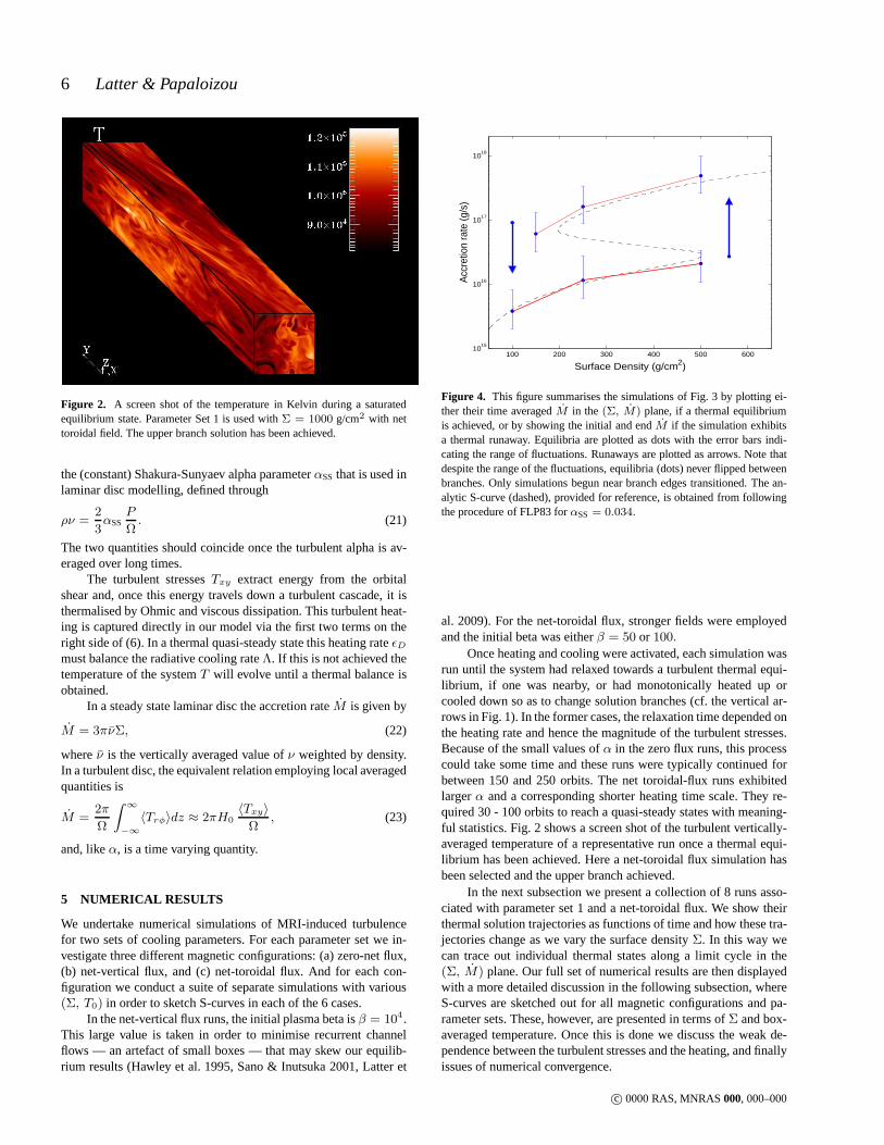
Figure 2. A screen shot of the temperature in Kelvin during a saturatedequilibrium state. Parameter Set 1 is used withΣ = 1000 g/cm2 with nettoroidal field. The upper branch solution has been achieved.

the (constant) Shakura-Sunyaev alpha parameterαSS that is used inlaminar disc modelling, defined through

ρν =2

3αSS

P

Ω. (21)

The two quantities should coincide once the turbulent alphais av-eraged over long times.

The turbulent stressesTxy extract energy from the orbitalshear and, once this energy travels down a turbulent cascade, it isthermalised by Ohmic and viscous dissipation. This turbulent heat-ing is captured directly in our model via the first two terms ontheright side of (6). In a thermal quasi-steady state this heating rateǫDmust balance the radiative cooling rateΛ. If this is not achieved thetemperature of the systemT will evolve until a thermal balance isobtained.

In a steady state laminar disc the accretion rateM is given by

M = 3πνΣ, (22)

whereν is the vertically averaged value ofν weighted by density.In a turbulent disc, the equivalent relation employing local averagedquantities is

M =2π

Ω

∫

∞

−∞

〈Trφ〉dz ≈ 2πH0

〈Txy〉

Ω, (23)

and, likeα, is a time varying quantity.

5 NUMERICAL RESULTS

We undertake numerical simulations of MRI-induced turbulencefor two sets of cooling parameters. For each parameter set wein-vestigate three different magnetic configurations: (a) zero-net flux,(b) net-vertical flux, and (c) net-toroidal flux. And for eachcon-figuration we conduct a suite of separate simulations with various(Σ, T0) in order to sketch S-curves in each of the 6 cases.

In the net-vertical flux runs, the initial plasma beta isβ = 104.This large value is taken in order to minimise recurrent channelflows — an artefact of small boxes — that may skew our equilib-rium results (Hawley et al. 1995, Sano & Inutsuka 2001, Latter et

100 200 300 400 500 60010

15

1016

1017

1018

Surface Density (g/cm2)

Acc

retio

n ra

te (g

/s)

Figure 4. This figure summarises the simulations of Fig. 3 by plotting ei-ther their time averagedM in the (Σ, M) plane, if a thermal equilibriumis achieved, or by showing the initial and endM if the simulation exhibitsa thermal runaway. Equilibria are plotted as dots with the error bars indi-cating the range of fluctuations. Runaways are plotted as arrows. Note thatdespite the range of the fluctuations, equilibria (dots) never flipped betweenbranches. Only simulations begun near branch edges transitioned. The an-alytic S-curve (dashed), provided for reference, is obtained from followingthe procedure of FLP83 forαSS = 0.034.

al. 2009). For the net-toroidal flux, stronger fields were employedand the initial beta was eitherβ = 50 or 100.

Once heating and cooling were activated, each simulation wasrun until the system had relaxed towards a turbulent thermalequi-librium, if one was nearby, or had monotonically heated up orcooled down so as to change solution branches (cf. the vertical ar-rows in Fig. 1). In the former cases, the relaxation time depended onthe heating rate and hence the magnitude of the turbulent stresses.Because of the small values ofα in the zero flux runs, this processcould take some time and these runs were typically continuedforbetween 150 and 250 orbits. The net toroidal-flux runs exhibitedlargerα and a corresponding shorter heating time scale. They re-quired 30 - 100 orbits to reach a quasi-steady states with meaning-ful statistics. Fig. 2 shows a screen shot of the turbulent vertically-averaged temperature of a representative run once a thermalequi-librium has been achieved. Here a net-toroidal flux simulation hasbeen selected and the upper branch achieved.

In the next subsection we present a collection of 8 runs asso-ciated with parameter set 1 and a net-toroidal flux. We show theirthermal solution trajectories as functions of time and how these tra-jectories change as we vary the surface densityΣ. In this way wecan trace out individual thermal states along a limit cycle in the(Σ, M) plane. Our full set of numerical results are then displayedwith a more detailed discussion in the following subsection, whereS-curves are sketched out for all magnetic configurations and pa-rameter sets. These, however, are presented in terms ofΣ and box-averaged temperature. Once this is done we discuss the weak de-pendence between the turbulent stresses and the heating, and finallyissues of numerical convergence.

c© 0000 RAS, MNRAS000, 000–000

Hysteresis in MRI simulations 7

0 20 40 60 80 1000

2

4x 10

16M

dot (

g/s)

0 20 40 60 80 1000

2

4x 10

16

0 20 40 600

2

4x 10

16

Mdo

t (g/

s)

0 10 20 30 400

1

2

x 1017

0 20 40 60 80 1000

5

10x 10

17

Mdo

t (g/

s)

0 20 40 60 80 1000

5

10x 10

17

0 20 40 600

1

2x 10

17

Time (orbits)

Mdo

t (g/

s)

0 2 4 6 8 100

5

x 1016

Time (orbits)

Σ=100 (LB) Σ=250 (LB)

Σ=500 (LB)

Σ=560 (LB)

Σ=500 (UB)

Σ=250 (UB)

Σ=150 (UB)

Σ=100 (UB)

Figure 3. The time evolution of the mass accretion rateM in eight simulations for the case of net toroidal-flux and parameter set 1. Hereβ = 100. Eachsimulation is distinguished by its (conserved) surface density Σ in cgs units. In a sequence running from left to right and top to bottom, the conserved surfacedensity moves first through increasing values for which there is a mean steady state corresponding to the lower branch (LB) of the S-curve plotted in Fig. 4.The simulation that is second from the top and on the right then moves to the upper branch (UB) as there is no available mean steady state on the lowerbranch. The sequence resumes with states of decreasing surface density tracing out the hot high-accreting solution on the upper branch. The final bottom rightsimulation then transitions to the lower branch, there being no steady state available on the upper branch for its lowΣ.

5.1 Simulation tracks in the (Σ, M) plane

In laminar disc modelling it is common to describe local S-curvesand limit cycles within the phase plane ofΣ andM because it is theaccretion rateM that dominates the state of the disc. Accordingly,we begin by discussing a subset of our simulation results in termsof the evolution ofM .

In Fig. 3 we plot the evolution tracks of eight simulations withnet-toroidal flux, withβ = 100, and parameter set 1. The sim-ulations differ in their (conserved) surface densityΣ and initialtemperatureT0. The simulations achieve either a thermal quasi-steady equilibrium near their initial state, in whichM fluctuatesabout a well-defined mean value, or they catastrophically heat upor cool down from their initial state, with an accompanying in-crease/decrease inM . These results are summarised by Fig. 4 inthe (Σ, 〈M〉) plane, where the〈M〉 of each simulation is com-

puted from a time average over the course of the run. Runs thatachieved a thermal steady state near their initial condition are rep-resented as dots with error bars showing the range of the fluctua-tions inM . Runs that evolved significantly away from their initialcondition are represented by arrows, the base of which denote theirstarting point and the tip of which their end point when the simula-tion was terminated.

As we progress from left to right and top to bottom throughthe eight panels in Fig. 3 we track the S-curve in Fig. 4 startingat the bottom left corner. First we travel towards the right along thelower branch, then up to the higher branch, then to the left along theupper branch, and finally back down to the lower branch. For thefirst three simulations/panels, the surface densityΣ moves throughincreasing values, each of which permits a cool low-accreting equi-librium. But the fourth simulation rapidly migrates from the vicin-ity of the lower branch: no cool low-accreting steady state is avail-

c© 0000 RAS, MNRAS000, 000–000

8 Latter & Papaloizou

able, because it possesses aΣ that is too large. It instead heats upand approaches an upper branch of hot solutions characterised byefficient accretion. The sequence then resumes with a procession ofhot equilibria with decreasingΣ. The eighth simulation transitionsfrom the vicinity of the upper branch to the lower branch as thereis no hot high-accreting state available that corrrespondsto its lowsurface density.

Though asingle run in local geometry cannot describe a com-plete limit cycle from beginning to end, our sequence ofmultipleruns can describe the constituent parts of a cycle, state by state.This is permitted because of the separation of time-scales betweenthe fast turbulent/thermo dynamics that determine the equilibria(& 1/Ω ∼ 103 s) and the slow dynamics of the cycle, which isgoverned by the accretion rate (& 1/(αΩ) ∼ 105 s).

Despite the large range of theM fluctuations witnessed inFig. 4 there is never any danger that the equilibrium states sponta-neously undergo transitions. States on the lower and upper branchesare robust and distinct, with their stability tied to (the smaller) vari-ations inT rather thanM . This point is is more apparent when theS-curves are plotted in the(Σ, T ) plane (see next subsection).

Finally, we have superimposed on Fig. 4 an analytic S-curvecomputed using the formalism of FLP83 with a Shakura-Sunyaevalpha ofαSS = 0.034. The location of the two numerical branchesand the stable analytic branches is reasonably consistent.However,the numerical branches often seem more extended to the right.

5.2 Thermal equilbria: S-curves as viewed in the (Σ, 〈T 〉)plane

In this subsection we present the bulk of our simulation resultsand plot S-curves for the cases of both parameter sets and forallthree magnetic field configurations. The same qualitative behaviouremerges in every scenario, which reinforce the robustness of thesefeatures.

Tables 1 and 2 summarise the simulation results and set-upfor the runs that quickly established thermal equilibria. Simulationswhich underwent a thermal evolution, corresponding to either sec-ular heating or cooling, are described in Tables 3 and 4. In Figs 5and 6 we plot S-curves for the various runs. These show the time-averaged temperature (once thermal equilibrium is achieved) as afunction of surface densityΣ (a conserved input parameter). Thefigures graphically summarise some of the data in Tables 1-4.Asin Fig. 4, the blue points with error bars represent the runs whichwere begun near a stable thermal equilibrium. The arrows repre-sent ‘thermally unstable’ runs, which were begun at the baseofeach arrow and were evolved to a state at the tip of each arrow,at which point the simulation either approached a stable branch orwas stopped.

First, the simulations reveal that the volume averaged temper-ature fluctuations in the turbulent equilibria are relatively small,some 10%, much smaller than forM . This means that the ther-mal equilibria are in fact very stable: turbulent fluctuations are notso extreme as to push the system over the unstable intermediatebranch in the(Σ, T ) diagram. In all the cases we simulate, equilib-rium states never jump branches spontaneously. Only at the ‘cor-ners’ of the S-curve is this a prospect. And on each corner thesys-tem could only move in one direction. As a consequence, limitcy-cle behaviour should follow broadly along the lines predicted bythe classical theory.

The ‘runaway’ simulations represent the system switching

branches on account of the fact that no equilibrium state wasavail-able. The simulations that went from the vicinity of the lower toupper branches heated up at a rateαΩ, as expected. The simula-tions that left the vicinity of the upper branch cooled at a varyingrate determined byΛ. In some cases turbulence in the latter simu-lations died out once the volume averaged temperature in theboxachieved a level much lower than the starting temperatureT0. Thisis because the scale height in the box becomes so small (of order thedissipation scale) that the MRI is suppressed. Similarly, the physi-cal condition of the gas becomes mismatched to the box size whenthe simulations catastrophically heat up. Simulations in both caseswere discontinued once this occurred.

Local simulations that begun near the S-curve ‘corners’ wouldoften bobble around indeterminately before switching curves. Inthese cases the system was near criticality and therefore small fluc-tuations in the heating rate change the stability of the system un-ceasingly. A sudden change in heating may cause the local equi-librium to vanish; the gas heats up or cools only for the heatingto readjust and the equilibrium state to reappear. It follows that in alimit cycle the branch jumping near branch ends can have a stochas-tic component. However, we reiterate we do not see such transitionsbetween thecentral regions of the upper and lower branches.

Superimposed upon the numerical S-curves are representa-tive analytical S-curves derived from FLP83, in whichαSS is auser defined parameter. TheseαSS values were chosen so that goodagreement was obtained with the numerical equilibria on thelowerbranch. Note, in particular, that once we set the analytic curves tomatch the lower equilibria, the upper numerical equilibriatend toexhibit slightly higher temperatures than expected from the analyticS-curves. Quite generally, the upper numerical branch is better ap-proximated by alpha models with largerαSS values than requiredon the lower branches. This could reflect the fact that the effectof turbulent heating is not accurately described by the classicalαmodel given the run times of the simulations. However, it couldalso to some extent reflect a bias in the way the simulations wereset up and carried out.

A close study indicates that the turbulentα weakly dependson the ratio of the average temperature〈T 〉 to the reference tem-peratureT0, or equivalently the mean scale height to the referencescaleH0. Very ‘hot’ (small) boxes withT > T0 exhibit a smallerα,while ‘colder’ (large) boxes yield largerα, with relative differences∼ 30%. This is essentially a numerical effect arising from varia-tions in the effective Reynolds number and it can operate withinany simulation. As a consequence, there is some low level indeter-minacy in both the properties of the equilibrium solutions and theexact locations of the S-curve corners. Their existence andgrossproperties, however, remain. Another, less important, consequenceof this ‘alpha feedback’ is the larger amplitude and intermittentthermal fluctuations in the saturated turbulent states, as comparedto isothermal models.

We remark that the need for a branch-dependentα, in the con-text of α disc modelling, was recognised early in order to obtaindecent matching of outburst behaviour with observations (Smak1984a, Lasota 2001). However, for the reasons mentioned above,caution should be exercised in the interpretation of our numericallocalα determinations in this context. Finally, note that the levelsof turbulence and values ofα increase with imposed toroidal orvertical magnetic flux. Thus if the flux were to increase as a systemtransitioned from a low state to a high state, the higher state wouldbe associated with a larger value ofα. Thus global disc simulations,

c© 0000 RAS, MNRAS000, 000–000

Hysteresis in MRI simulations 9

200 400 600 800 1000 1200 1400 1600 1800 200010

3

104

105

Surface Density (g /cm2)

Mid

pla

ne

Te

mp

era

ture

(K

)S−curve from Zero−flux MRI simulations

100 200 300 400 500 600 700 800 900 1000 1100

104

105

Surface Density (g/cm2)

Mid

pla

ne

Te

mp

era

ture

(K

)

S−curve from vertical flux MRI simulations

100 200 300 400 500 600 700 800 900 1000 1100

104

105

Surface Density (g/cm2)

Mid

pla

ne

Te

mp

era

ture

(K

)

S−curve from toroidal flux MRI simulations

Figure 5. S-curves computed with ZEUS for parameter set 1:(µ, E, λ) = (1, 3.5, 5) and for the three magnetic configurations. The first panel correspondsto zero net-flux, the second panel to net vertical-flux (initial β = 104), and the third panel to a net toroidal-flux (initialβ = 100). Simulation results areindicated on the(Σ, Tc) plane, withTc, in K, evaluated as the volume average of the temperature,T, over the box.Σ is expressed in cgs units. Runs thatattained an approximate quasi-steady state are indicated by a dot, corresponding to the time average mean volume averagedT , and with errorbars, indicatingthe maximum and minimum volume averagedT once the steady state is achieved. Cases indicated with arrows pointing upward/downward underwent aheating/cooling instability, with the volume averagedT on average showing a monotonic increase/decrease with time. Notation is otherwise the same asin Fig. 4. The dashed curves represent equilibrium S-curvescalculated using the formalism of FLP83 forαSS = 0.007, 0.0275, 0.034 for the zero flux,net-vertical flux, and toroidal flux cases respectively.

for which net-flux need not be conserved locally, could potentiallylead to such localα variations.

5.3 Turbulent stresses and heating

We compared the box averaged pressure (and temperature) withthe turbulent stress in our quasi-steady equilibria. In Fig. 7 we plota representative evolution of these two fluctuating quantities. As isclear, on the orbital time-scale there only exists a weak dependencebetween pressure and the turbulent stress (described byα). There

are three discrepancies. First, pressurelags behind the turbulentstress by roughly an orbit, which indicates that on short times thecausal relationship is from viscous stress to pressure and not theother way around, in agreement with Hirose et al. (2009). Peaksin α describe intense large-scale events, the energy of which sub-sequently tumbles down a cascade to reach dissipative scales. Thegas heats up and the pressure increases. This process, however, isnot instantaneous and the originalα signal is significantly modi-fied (‘smoothed-out’) by the time that it manifests itself asheating(see Pearson et al. 2004 for similar results in forced isotropic tur-

c© 0000 RAS, MNRAS000, 000–000

10 Latter & Papaloizou

100 200 300 400 500 600 700 800 900 1000 1100

104

105

Surface Density (g/cm2)

Mid

pla

ne

Te

mp

era

ture

(K

)S−curve from zero net flux MRI simulations

50 100 150 200 250 300 350

104

105

Surface Density (g/cm2)

Mid

pla

ne

Te

mp

era

ture

(K

)

S−curve from vertical flux MRI simulations

50 100 150 200 250 300

104

105

Surface Density (g/cm2)

Mid

pla

ne

Te

mp

era

ture

(K

)

S−curve from toroidal flux MRI simulations

Figure 6. S-curves computed with NIRVANA and ZEUS for the second parameter set:(µ, E, λ) = (0.5, 5.66, 1). The first panel corresponds to zero net-flux, the second panel to net vertical-flux (initialβ = 104), and the third panel to a net toroidal-flux (initialβ = 50). The dashed curves represent equilibriumS-curves calculated using the formalism of FLP83, withαSS = 0.009, 0.0475, 0.07 for the zero flux, net-vertical flux, and toroidal flux cases respectively.Notation is otherwise the same as in Fig. 5.

bulence). Second, the volume averaged pressure andα time seriesare dissimilar; in particular, the volume averaged pressure appearsat best as a heavily convolved version ofα. Lastly, variations inα are much larger than related variations in the volume averagedpressure, which are relatively mild, with the former∼30%, and thelatter less than5%.

This poor correlation between the viscous stress and pressureon short times casts doubt on the existence of thermal instabili-ties that rely on these two quantities to be functionally dependent(Shakura & Sunyaev 1976, Abramowicz et al. 1988). Indeed, nu-merical simulations of the MRI in radiation pressure dominateddiscs reveal no thermal instability (Hirose et al. 2009). Recently,linear stability analyses have been conducted that allow the pres-sure to lag behind stress, and vice-versa. These show that, de-

spite this impediment, instability can in fact persist, especially withthe short time-lags witnessed in our simulations (Lin et al.2011;Ciesielski et al. 2012). It would appear then that the main obsta-cle to instability in turbulent models of discs is due to somethingelse, perhaps the stochastic nature of the viscous stress which isnot faithfully reproduced in the behaviour of the volume averagedpressure (Janiuk and Misra 2012).

Finally, note that overlong times the turbulent stressTxy andpressureare correlated. Thus turbulent accretion on the hot upperbranch of equilibria is greater than accretion in the colderstates (cf.Section 5.1).

c© 0000 RAS, MNRAS000, 000–000

Hysteresis in MRI simulations 11

Paramater Set 1: Thermal quasi-equilibrium

B Configuration Σ 〈T 〉 max(T ) min(T ) α Orbits

Zero Vertical (l.b.)

500 2.74× 103 2.91× 103 2.57× 103 0.0062 2401000 2.79× 103 3.42× 103 2.61× 103 0.0049 1701200 3.16× 103 3.51× 103 2.89× 103 0.0081 3501400 3.52× 103 3.99× 103 2.89× 103 0.0076 1901500 4.10× 103 5.12× 103 2.89× 103 0.0079 300

Zero Vertical (u.b.)

600 5.92× 104 6.26× 104 5.70× 104 0.0084 180800 6.97× 104 7.30× 104 6.78× 104 0.0083 901000 8.14× 104 8.95× 104 7.69× 104 0.0098 1901600 10.1× 104 10.5× 104 9.83× 104 0.0082 1302000 11.5× 104 12.7× 104 10.6× 104 0.010 170

Net Vertical (l.b.)

200 2.93× 103 3.05× 103 2.83× 103 0.0348 80300 3.16× 103 3.35× 103 3.00× 103 0.0342 40350 3.25× 103 3.68× 103 3.04× 103 0.0359 90400 3.35× 103 3.68× 103 3.17× 103 0.0368 80500 3.71× 103 4.50× 103 3.33× 103 0.0387 105550 4.56× 103 6.27× 103 3.33× 103 0.0384 160575 4.26× 103 5.09× 103 3.33× 103 0.0355 100

Net Vertical (u.b.)

200 3.66× 104 4.11× 104 3.16× 104 0.0362 65400 5.99× 104 6.87× 104 5.46× 104 0.0351 140650 7.95× 104 8.79× 104 7.52× 104 0.0375 481000 10.1× 104 11.1× 104 9.43× 104 0.038 90

Net Toroidal (l.b.)100 3.27× 103 3.44× 103 3.16× 103 0.0476 110250 3.74× 103 4.37× 103 3.46× 103 0.0507 110500 4.01× 103 4.33× 103 3.86× 103 0.0422 75

Net Toroidal (u.b.)

150 3.72× 104 4.12× 104 3.35× 104 0.0442 65250 5.36× 104 5.82× 104 5.04× 104 0.0487 118500 7.99× 104 8.53× 104 7.54× 104 0.0491 110750 9.97× 104 10.6× 104 9.52× 104 0.0491 1051000 10.3× 104 10.9× 104 9.97× 104 ... 65

Table 1. Summary of the inputs and average values of simulations undertaken by ZEUS with parameter set 1:µ = 1, E = 3.5, λ = 5. The magnetic fieldconfiguration is varied as is the input surface densityΣ. The initial β is 104 for the net vertical field runs, and 100 for the net toroidal field runs. Quasi-steadythermal equilibria are attained that align with one of the two stable branches of the S-curve, with ‘l.b.’ denoting ‘lower branch’, and ‘u.b.’ denoting ‘upperbranch’.

5.4 Numerical convergence

Finally, we briefly discuss issues associated with the numerics. Pa-rameter set 1 was primarily undertaken with ZEUS and parameterset 2 with NIRVANA, however the two codes were run on an over-lap set of some 8 simulations. The comparison yielded good agree-ment in both〈T 〉 andα, with discrepancies within the range of thefluctuations. It follows that not only are our qualitative results ro-bust with respect to parameter choices and magnetic configurations,they are robust with respect to numerical method.

In addition, we performed a short study in order to confirmthat the simulations were adequately converged with respect toresolution and Reynolds number. A representative sample ofrunswere taken and we evaluated the quantitiesα and〈T 〉 for differentReynolds numbers while keeping the Prandtl number constantandequal to 4. In summary we found that doubling the kinematic vis-cosityν (halving the Reynolds number) led to changes inα and〈T 〉that were less than5%. This reproduces the very weak Reynoldsnumber dependence uncovered by Fromang (2010). Moreover, theresult held whether we took 64 grid points perH0 or 128 points.

Thus we were assured that these quantities were satisfactorily con-verged.

Next we kept the diffusion coefficients fixed and varied theresolution. We evaluated the above quantities at both 64 and128grid cells perH0. The lower resolution runs yielded slightly lower〈T 〉 but the discrepancy was within10%. This small decline is un-derstandable because at coarser resolutions more of the turbulentenergy is removed by the grid and thus less captured by physi-cal Ohmic and viscous heating. As a consequence, there is slightlyless direct heating. That said, the effect is small and in general nogreater than the statistical fluctuations of the runs. It leads in noway to any change in the qualitative behaviour exhibited.

6 CONCLUSION

In this paper we performed a suite of numerical simulations of theMRI in local geometry with the ZEUS and NIRVANA codes. Bothviscous and Ohmic heating is included, while the radiative cool-ing is approximated by a physically motivated cooling function

c© 0000 RAS, MNRAS000, 000–000

12 Latter & Papaloizou

Parameter Set 2: Thermal quasi-equilibrium

B Configuration Σ 〈T 〉 max(T ) min(T ) α Orbits

Zero Vertical (l.b.)

100 3.51× 103 3.65× 103 3.36× 103 0.0092 120300 3.74× 103 3.97× 103 3.51× 103 0.0095 180400 3.82× 103 4.25× 103 3.50× 103 0.014 334500 3.95× 103 4.07× 103 3.74× 103 0.0095 123650 4.72× 103 5.35× 103 4.07× 103 0.011 197750 4.84× 103 5.35× 103 2.55× 103 0.0105 176

Zero Vertical (u.b.)

300* 3.27× 104 4.63× 104 2.04× 104 0.011 211300** 4.64× 104 5.24× 104 4.03× 104 0.012 185400† 5.52× 104 5.74× 104 4.97× 104 0.0095 221400†† 5.60× 104 6.12× 104 5.09× 104 0.011 226500 6.18× 104 6.37× 104 5.98× 104 0.0095 90

Net Vertical (l.b.)

80 3.90× 103 4.08× 103 3.74× 103 0.036 70100 4.11× 103 4.80× 103 3.83× 103 0.0425 67150 3.99× 103 4.06× 103 3.92× 103 0.038 33200 4.14× 103 4.24× 103 4.03× 103 0.041 33250 4.83× 103 5.19× 103 4.46× 103 0.042 35

Net Vertical (u.b.)

140 3.49× 104 4.08× 104 2.89× 104 0.045 67160 3.99× 104 4.67× 104 3.31× 104 0.041 40200 4.33× 104 4.75× 104 3.90× 104 0.028 59250 5.7× 104 6.12× 104 5.28× 104 0.038 25300 6.0× 104 6.34× 104 5.66× 104 0.042 27

Net Toroidal (l.b.)80 4.20× 103 4.33× 103 4.07× 103 0.061 38100 4.31× 103 4.43× 103 4.20× 103 0.068 50130 4.41× 103 4.54× 103 4.30× 103 0.071 34170 4.89× 103 5.03× 103 4.68× 103 0.08 44200 5.47× 103 5.87× 103 5.10× 103 0.072 44

Net Toroidal (u.b.)

100 3.31× 104 3.63× 104 3.02× 104 0.085 43140 4.49× 104 4.69× 104 4.24× 104 0.075 45160 4.84× 104 5.20× 104 4.58× 104 0.072 37200 5.18× 104 5.73× 104 4.88× 104 0.054 37

Table 2. Summary of the inputs and average values for simulations undertaken by NIRVANA adopting parameter set 2:µ = 1, E = 5.66, λ = 1. The initialβ is 104 for the net vertical field runs, and 50 for the net toroidal field runs. Some simulations are performed with the same value ofΣ but different initialmean temperatures: * indicates a run begun with〈T 〉 = 3.85× 104, whereas ** indicates〈T 〉 = 4.75× 104; † denotes an initial〈T 〉 = 5.20× 104 and††denotes〈T 〉 = 6.00 × 104 . The larger variations associated with the former pair of cases occurs because the steady state thermal equilibrium is expected tobe located near the upper bend in theS curve.

that summarises the strong effect of temperature on the ability ofthe disc gas to retain heat. Different magnetic configurations (zeroflux, net-toroidal flux, net-vertical flux) and parameters were tri-aled, with little change in the qualitative results.

Our simulations unambiguously exhibit the development ofthermal instability and hysteresis. In particular, through a sequenceof runs we can sketch out characteristic S-curves in the phase spaceof (Σ, Tc) and(Σ, M), which are central to the classical outburstmodel. It hence appears that MRI turbulence is not so intermittentas to endanger the robustness of the cycle. Temperature fluctuationsare well-behaved and relatively small and there is no spontaneousjumping from one stable branch to the other. Only near the ‘cor-ners’ of the S-curve does significant stochasticity enter, as then theexistence or not of a local equilibrium is uncertain. This featurewill add some degree of low level ‘noise’ to the observed outbursttime-series. In addition, theα we record on the two stable branchesdiffer slightly but systematically. Because of the constraints of ourlocal model, this result is more suggestive than anything else. How-

ever, it does indicate that in global disc simulations we mayindeedsee a systematic difference in the two branches, as requiredby theclassical theory.

Finally, on the orbital time the turbulent stresses and pressureonly weakly depend on each other in our simulations. Pressure al-ways lags behind the turbulent stress, and thus the causality is fromthe stress to the pressure, via the turbulent heating (in agreementwith Hirose et al. 2009). Moreover, the pressure response isa sig-nificantly ‘smoothed out’ echo of the turbulent stress features. Bothfacts indicate that thermal instability driven by turbulent heatingvariations, in which the stress is a function of pressure, may notoperate in real discs. On long times, however, there is necessarilya feedback of the pressure on the stress, which leads to differentaccretion rates on the two branches of the S-curve.

Our work presents a first step towards unifying simulations offull MHD turbulence with the correct thermal and radiative physicsof outbursting DNe and LMXBs, and possibly young stellar ob-jects. We have begun with with the most basic model that yields

c© 0000 RAS, MNRAS000, 000–000

Hysteresis in MRI simulations 13

Parameter Set 1: Thermal runaways

B Configuration Σ initial T final T Orbits

Zero Vertical (c)300 3.7× 104 6.0× 103 60400 4.0× 104 3.5× 103 125500 4.75 × 104 2.7× 103 178

Zero Vertical (h) 1700 4.5× 103 3.4× 104 535

Net Vertical (c)150 4.8× 104 6.3× 103 20175 6.5× 104 7.1× 103 31188 6.0× 104 7.8× 103 52

Net Vertical (h)600 3.3× 103 1.1× 104 101650 3.3× 103 1.4× 104 108

Net Toroidal (c) 100 5.0× 104 9.0× 103 14

Net Toroidal (h)560 3.6× 103 2.5× 104 43625 3.6× 103 4.1× 104 73750 3.0× 103 4.4× 104 68

Table 3. Summary of the inputs and range of values found for simulationsundertaken ZEUS adopting parameter set 1:µ = 1, E = 3.5, λ = 5.The magnetic field configuration is varied as is the input surface densityΣ.These simulations resulted in thermal runaways, i.e. persistent heating orcooling as indicated by either (h) or (c) . This is because they were initiallylocated near the corners ofS curves in the surface density time averagedmean temperature plane. In the latter case this occured on a time scale of afew orbits in some simulations. In general very large changes to the meantemperature in these simulations eventually resulted in the computationalbox becoming mismatched to the putative scale height. Accordingly, theywere then not continued.

Parameter Set 2: Thermal runaways

B Configuration Σ initial T final T Orbits

Zero Vertical (c)100 3.18 × 104 3.18× 103 5.6186 3.18 × 104 3.19× 103 17

Zero Vertical (h)

686 8.49 × 103 1.70× 104 270850 6.34 × 103 1.78× 104 155950 4.75 × 103 1.50× 104 541000 6.37 × 103 4.07× 104 1191100 2.00 × 103 1.17× 104 921200 6.00 × 103 3.18× 104 2541200 8.00 × 103 5.92× 104 215

Net Vertical (c)80 3.82 × 104 6.37× 103 3.8100 3.18 × 104 5.31× 103 5.25

Net Vertical (h)275 2.00 × 103 1.62× 104 81300 1.27 × 104 1.78× 104 33

Net Toroidal (c) 80 3.82 × 104 1.59× 104 5.9

Net Toroidal (h)225 4.00 × 103 5.56× 104 66250 9.55 × 103 1.46× 104 43

Table 4. As in table 3 but for simulations undertaken by NIRVANA andZEUS adopting parameter set 2:µ = 0.5, E = 5.66, λ = 1.

76 77 78 79 80 81 82 83 84 850.04

0.05

0.06

0.07

0.08

0.09

0.1

α

76 77 78 79 80 81 82 83 84 850.76

0.78

0.8

0.82

0.84

Time (orbits)

<P>/

P0

Figure 7. Plots of the turbulent stress, quantified byα, versus time andthe volume averaged pressure versus time. Parameters correspond to Set 1;there is a net toroidal-flux associated with initialβ = 100, andΣ = 250(UB) (see Table 1). It is clear that the latter tracks the stress imperfectly,with much of the short time scale stochastic variability seen in the stresswashed out. Gross features are also associated with a time-lag of about anorbit.

the correct physics: local simulations of gas inhabiting a singleradius in the disc with a simple radiative prescription. This is a‘ground zero’ test of the compatibility of the MRI with the puta-tive thermal limit cycles of outbursting discs. If MRI-turbulencehad failed in this basic setting it would probably fail in more ad-vanced models as well. Now that we are assured of this compatabil-ity, a variety of further work may be attempted. For instance, sim-ulations could be performed in vertically stratified shearing boxeswith more realistic radiation physics (in the flux-limited diffusionapproximation with appropriate opacities). In addition, cylindricalMRI simulations should be performed with the FLP83 cooling pre-scription, anologous to the globalα disc calculation of Papaloizouet al. (1983). Such simulations would describe how real turbulencemediates the heating and cooling fronts that propagate through thedisc during a transition between branches.

ACKNOWLEDGMENTS

The authors thank the anonymous referee for his review andSebastien Fromang for his comments on an earlier versionof the manuscript. This work was supported by STFC grantST/G002584/1 and the Cambridge high performance computingservice DARWIN cluster. HNL thanks Tobias Heinemann andPierre Lesaffre for coding tips.

REFERENCES

Abramowicz, M. A., Czerny, B., Lasota, J. P., Szuszkiewicz,E., 1988. ApJ,332, 646.

Armitage, P. J., Livio, M., Pringle, J. E., 2002. MNRAS, 324,705.Balbus, S. A., Hawley, J. F., 1992. ApJ, 400, 610.Balbus, S. A., Hawley, J. F., 1998. RvMP, 70, 1.Balbus, S. A., Papaloizou, J. C. B., 1999. ApJ, 521, 650.Bell, K. R., Lin, D. N. C., 1994. ApJ, 427,987.Ciesielski, A., Wielgus, M., Kluzniak, W., Sadowski, A., Abramowicz, M.,

Lasota, J.-P., Rebusco, P., 2012. AA, 538, 148.Faulkner, J., Lin, D. N. C., Papaloizou, J., 1983. MNRAS, 205, 359.Ferreira, B. T., Ogilvie, G. I., 2009. MNRAS, 392, 428.

c© 0000 RAS, MNRAS000, 000–000

14 Latter & Papaloizou

Fromang, S., 2010. AA, 514, L5.Fromang, S., Papaloizou, J., Lesur, G., Heinemann, T., 2007. AA, 476,

1123.Gallagher, J. S., Starrfield, S., 1978. AA, 12 171.Gammie, C. F., 1996. ApJ, 553, 174.Goldreich, P., Lynden-Bell, D., 1965. MNRAS, 130, 125.Hawley, J. F., 2000. ApJ, 528, 462.Hawley, J. F., Gammie, C. F., Balbus, S. A., 1995. ApJ, 440, 742.Hayashi, C., Hoshi, R., 1961. PASJ, 13, 450.Hirose, S., Krolik, J. H., Blaes, O., 2009. ApJ, 691, 16.Hoshi, R., 1979. Prog. Theor. Phys. 61, 1307.Ichikawa, S., Osaki, Y., 1992. PASJ, 44, 15.Janiuk, A., Misra, R., 2012. AA accepted, (arXiv:1203.0139).Kato, S, 2003. PASJ, 55, 801.Lasota, J.-P., 2001. New Astr. Rev. 45, 449.Lasota, J.-P., 2012. In: Eds Giovannelli, F., Sabau-Graziati, L., The

Golden Age of Cataclysmic Variables and Related Objects, inpress(arXiv:1111.0209)

Latter, H. N., Lesaffre, P., Balbus, S. A., 2009. MNRAS, 394,715.Lesaffre, P., Balbus, S. A., 2007. MNRAS, 381, 319.Lesaffre, P., Balbus, S. A., Latter, H. N., 2009. MNRAS, 396,779.Lightman, A. P., Eardley, D. M., 1974. ApJ, 187, L1.Lin, D.-B, Gu, W.-M., Lu, J.-F., 2011. MNRAS, 415, 2319.McClintock, J. E., Remillard, R. A., 2006. In: Eds Lewin, W.,van der Klis,

M., Compact stellar X-ray sources, Cambridge AstrophysicsSeries,No. 39. Cambridge Uni. Press, Cambridge UK.

Menou, K., Hameury, J.-M, Stehle, R., 1999. MNRAS, 305, 79.Meyer, F., Meyer-Hofmeister, E., 1981. A&A, 104, L10Meyer, F., Meyer-Hofmeister, E., 1984. A&A, 132, 143Papaloizou, J.C.B., Nelson, R.P., 2003. MNRAS, 339, 983.Osaki, Y., 1974. PASJ, 26, 429.Osaki, Y., 1994. PASJ, 26, 429.Papaloizou, J., Faulkner, J., Lin, D. N. C., 1983. MNRAS, 205, 487.Papaloizou, J. C. B., Pringle, J. E., 1984. MNRAS, 208, 721.Pearson, B. R., Yousef, T. A., Haugen, N. E. L., Brandenburg,A., Krogstad,

P.-A., 2004. PhRvE, 70, 6301.Pringle, J. E., 1981. ARAA, 19, 137.Sano, T., Inutsuka, S., 2001. ApJ, 561, L179.Shara, M. M., 1989. PASP, 101, 5.Shakura, N., I., Sunyaev, R. A., 1973. AA, 24, 337.Shakura, N., I., Sunyaev, R. A., 1976. MNRAS, 175, 613.Silvers, L. J., 2008. MNRAS, 385, 1036.Smak, J., 1971. AcA, 21, 15.Smak, J., 1984a. AcA, 34, 161.Smak, J., 1984b. PASJ, 96, 5.Starrfield, S., Sparks, W. M., Truran, J. W., Wiescher, M. C.,2000, ApJS,

127, 485.Stone, J. M., Norman, M., L., 1992a. ApJS, 80, 753.Stone, J. M., Norman, M., L., 1992b. ApJS, 80, 791.Stone, J. M., Hawley, J. F., Gammie, C. F., Balbus, S. A., 1996. ApJ, 463,

656.Warner, B., 1995. Cataclysmic variable stars. Cambridge Uni Press, Cam-

bridge UK.Zhu, Z, Hartmann, L., Gammie, C., McKinney, J. C., 2009. ApJ,701, 62.Zhu, Z., Hartmann, L., Gammie, C. F., Book, L. G., Simon, J. B., Engelhard,

E., 2010. ApJ, 713, 1134.Ziegler, U., 1999. CoPhC, 116, 65.

APPENDIX A: RADIATIVE COOLING MODEL

In this appendix we detail how the cooling prescription of Section3.2 was derived. In particular we show how the effective tempera-tureTe is calculated within each of the three important gas regimesintroduced.

A1 Regime 1: the optically thick hot regime

The radiative cooling function can be written as a flux in the diffu-sion approximation byΛ = ∇ · F where

F = −4acT 3

3κρ∇T, (A1)

in whichκ is the opacity,a = 4σ/c is the Stefan-Boltzmann radi-ation constant andc is the speed of light. Setting the optical depthas

τ =

∫

∞

z

κ(x, y, z′)ρ(x, y, z′)dz′, (A2)

we obtain the vertical component ofF in the form

Fz =4acT 3

3

∂T

∂τ. (A3)

We integrate from near the disc surface whereT = Te, (the effec-tive temperature), andτ = τe ∼ 1 to the mid plane wherez = 0,T = Tc andτ = τc. Thus we obtain

T 4

c − T 4

e =

∫ τc

τe

3Fz

acdτ, (A4)

whereTc is the mid plane temperature.In the hot optically thick Regime 1,τc ≫ τe ∼ 1 andT 4

c ≫T 4

e so that (A4) implies

T 4

c ∼

∫ τc

1

3Fz

acdτ ∼

3τc4

T 4

e , (A5)

where we have approximatedFz to be constant and equal to its sur-face valueacT 4

e /4. This equation relates the effective temperatureTe to the central temperatureTc.

To complete the prescription we take the scale height to be

H = (RTc/µ)1/2Ω−1, (A6)

and set the surface density to

Σ = 2ρcH. (A7)

Finally, as most of the optical depth arises from the regionsnear themidplane, we approximate Eq. (A2) by

τc = κcΣ/2, (A8)

whereκc is the opacity evaluated at the densityρc and the midplanetemperatureTc. In this hot ionised regime, we can approximateκby the following formula:

κ = 1.5 × 1020ρT−2.5, (A9)

(FLP83). So for specifiedΩ, the above relationships enableTe (andhenceΛ) to be related to conditions in the mid plane, and henceTc

andΣ.

A2 Regime 2: the warm transitional regime

This regime exhibits a cooler disc midplane that is still well ionisedbut surface layers that are. 5000 K, and which are poorly ionised.As a result, near the photosphereκ not only drops significantly butbecomes a steeply increasing function of temperature. It followsthat the requirementτ ∼ 1 at the photosphere determines the ther-mal structure of the disc, as in cool stars (Hayashi & Hoshi 1961).Instead of (A5) one must impose the conditionτe ≈ 1, whereτeis the optical depth at the location whereT = Te. As the optical

c© 0000 RAS, MNRAS000, 000–000

Hysteresis in MRI simulations 15

surface is∼ H above the mid plane, it converts to a relationshipbetween the disc surface densityTe andTc that leads to the centralunstable part of the S-curve when thermal equilibria are considered.

We introduce the quantityτ∗e which we define throughτ∗

e =κeΣ with κe being the opacity evaluated at thecentral densityρcbut with the photospheric temperatureTe. It is anticipated thatτ∗

e

overestimates the optical depth of material above the disc photo-sphereτe by some factor of order unity. This factor we quantifythrough the dimensionless constantE, so that

E τ∗

e = τe ≈ 1 (A10)

Once the dependence ofκe on Te and ρc is specified, equation(A10) supplies a means to obtainTe, and henceΛ, when the discis in Regime 2. Finally, an approximate functional form ofκ in thisregime of incomplete hydrogen ionisation is

κ = 10−36ρ1/3T 10, (A11)

(FLP83).

A3 Regime 3: the cool optically thin regime

In this regime the vertical structure of the disc is isothermal withT ≈ Tc. However, because the disc is optically thin in the verticaldirection,Fz is reduced fromacT 4

c /4 by a factor∼ 2τc. Thus weset

T 4

e = 2λτcT4

c , (A12)

whereλ is a dimensionless constant of order unity that takes ac-count of appropriate frequency averaging and any other necessarycorrections arising from a more complete discussion of radiationtransport. This condition also connectsTe to Tc andΣ. The centraloptical depth in this regimeτc is computed using Eq. (A8) and theopacity prescription introduced in Eq. (A11).

A4 Interpolated form

The prescription forTe is given in Eq. (11) for each of the threeregimes. In numerical simulations one could switch from oneformto the other according to the local value ofTc; we however em-ploy an analytic interpolation of the three forms, as in FLP83. InEq. (11), the effective temperatureTe takes one of three forms,which we denote by eitherT1, T2 or T3 where the subscript in-dicates the associated regime. These three functions are then inter-polated via the following:

T 4

e =(T 4

1 + T 4

2 )T4

3

[(T 4

1+ T 4

2)1/2 + T 2

3]2, (A13)

(FLP83). It is this algebraic expression forTe that is used in Equa-tion (10) to evaluateΛ. The two free parametersλ andE can bechosen to fit results obtained from vertical integrations with stan-dard localα modelling. In Fig. (A1) we plot the resulting func-tional dependence ofTe on the central temperatureTc with thethree regimes indicated on the curve. In regimes 1 and 3 the effec-tive temperature increases steeply with central temperature, whilein the transitional regime 2 the dependence is very weak on accountof the rapid changes in opacity near the surface. In this intermedi-ate regime the radiative cooling rate is very ‘flat’ and, consequently,thermal instability ensues (cf. Eq. (2)).

1 2 3 4 5 6 7 8

x 104

1000

2000

3000

4000

5000

6000

7000

8000

9000

Tc (Kelvin)

T e (K

elvi

n)

Regime 1

Regime 2

Regime 3

Figure A1. The effective temperatureTe as a function of central temper-atureTc as determined from the FLP83 cooling prescription, cf. Eq. (11).Parameters areµ = 1, E = 3.5 andλ = 5. In addition, we have indicatedon the curve which regime is dominant.

c© 0000 RAS, MNRAS000, 000–000