Hydrology - Campanastanaquadoc.typepad.com/files/campana_and_amin_1996.pdf · LE. Amin and M.E. Campana / Journal of Hydrology 179 (1996) 1-21 3 recognize that the proposed model

Journal of Hydrology

EI_~EVIER Journal of Hydrology 179 (1996) 1-21

A general lumped parameter model for the interpretation of tracer data and transit time calculation in hydrologic systems

Isam E. Amin a'*, Michael E. Campana b aDepartmem of Geological Sciences, California State University, 1250 Bellflower Boulevard, Long Beach,

CA 90840-3902, USA bDepartment of Earth and Planetary Sciences, Northrop Hall, University of New Mexico, Albuquerque,

NM 87131-1116, USA

Received 25 May 1994; revision accepted 23 July 1995

Abstract

We present a general lumped parameter mathematical model for hydrologic tracer data interpretation and mean transit time calculation in hydrologic systems. The model takes the form of the three-parameter gamma distribution and accounts for different mixing types: perfect mixing; no mixing (piston flow); partial mixing (dispersive mixing, or the type between perfect mixing and no mixing); and various eombinations of the above types. In these combinations, the different mixing types simulated by the model conceptually represent reservoirs in series. We introduce the mixing efficiency to characterize the extent or degree of natural mixing in hydrologic systems. This parameter equals zero for piston flow (no mixing), unity for perfect mixing, and a value in between these two extremes for partial mixing. The general model simulates the combination of perfect mixing, partial mixing, and piston flow. Six other models that simulate one or two of these mixing types can be obtained as special cases from the general model. Therefore, seven models are introduced in this effort. Of these, four (including the general model) are new, and three are currently existing in the field of tracer hydrology. The three existing models are the perfect mixing model, piston flow model, and the perfect-piston flow model which simulates the Combination of perfect mixing and pisto n flow. The new models are the perfect-partial-piston flow model (the general model), perfect-partial mixing model, partial-piston flow model, and partial mixing model.

Modeled mean transit times for three case studies agree with previous estimates: 21 and 2.4 years for two springs (sites 2 and 45, respectively) on Cheju Island, Republic of Korea; and 3.0 years for the Ottawa River basin, Canada.

* Corresponding author

0022-1694/96/$15.00 © 1996 - Elsevier Science B.V. All rights reserved SSDI 0022-1694(95)02880-3

2 LE. Amin and M.E. Carnpana / Journal of Hydrology 179 (1996) 1-21

1. Introduction

Tracers can be used to estimate hydrologic system parameters by means of mathematical models (transit time distribution functions) that relate the tracer input and output concentrations. The tracer concentration, however, is influenced by mixing owing to hydrodynamic dispersion in the hydrologic system. This effect is accounted for by assuming specific mixing regimes in the development of the models.

Mixing can range from piston flow (or no mixing) as a lower limit, to perfect (or complete) mixing as an upper limit. Perfect mixing, in general, is a characteristic of not-too-deep surface water systems (Kaufman and Libby, 1954), but is useful only as a limiting case for groundwater systems (Nir, 1964). Both perfect mixing and piston flow represent limiting cases that seldom occur in groundwater systems. It is most probable that the type of mixing encountered in groundwater systems, or natural hydrologic systems in general, lies somewhere between these two extremes. We call this type of mixing partial mixing.

Currently, the most widely used analytical models for simulating partial (dispersive) mixing are those that utilize the 'dispersivity' concept such as the dispersive model (Nir, 1964; Maloszewski and Zuber, 1982). However, reliable estimates of the dispersivity, which may be scale-dependent (Anderson, 1979; Wheatcraft and Tyler, 1988; Gelhar et al., 1992), are very difficult to obtain. The dispersive model is also characterized by other limitations. Zuber (1986a) pointed out that the theore- tical foundation for the dispersive model in its lumped-parameter form is not sound for systems other than packed beds (e.g. soil columns) or pipelines with turbulent or laminar flow. Partial mixing can be modeled by discrete-state compartment models (Przewlocki and Yurtsever, 1974; Campana, 1975; Simpson and Duckstein, 1976). Although discrete-state compartment models are capable of modeling spatially distributed systems, their major limitation is that they require a large number of fitting parameters.

In this study we develop a general lumped-parameter mathematical model which accounts for different types of mixing in steady and non-steady hydrologic systems: piston flow or no mixing, partial mixing, perfect mixing and their combinations (which represent the simultaneous existence of the three or any two of the mixing types in the system). The lumped parameter approach is the most common one used for quantitative interpretation of tracer data in hydrologic systems (Zuber, 1986a). The general model developed in this study simulates the combination of perfect mixing, partial mixing, and piston flow, where the mixing types occupy reservoirs in series. Six other models that simulate one or two of these mixing types can be obtained as special cases from the general model. Therefore, seven models are introduced in this study. Of these, four (including the general model) are new, and three currently exist in tracer hydrology. The three existing models are the perfect mixing model, piston flow model, and the perfect-piston flow model which simulates the combination of perfect mixing and piston flow. The new models are the perfect-partial- piston flow model (the general model), perfect-partial mixing model, partial-piston flow model, and partial mixing model.The general model follows the three-parameter gamma distribution. Hydrologists familiar with the Nash model (Nash, 1957) will

LE. Amin and M.E. Campana / Journal of Hydrology 179 (1996) 1-21 3

recognize that the proposed model takes the form of the Nash model if a time lag is added to the latter. However, the Nash model without a time lag does not give the four new models proposed in this study.

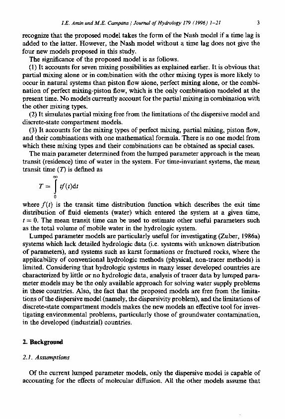
The significance of the proposed model is as follows. (1) It accounts for seven mixing possibilities as explained earlier. It is obvious that

partial mixing alone or in combination with the other mixing types is more likely to occur in natural systems than piston flow alone, perfect mixing alone, or the combination of perfect mixing-piston flow, which is the only combination modeled at the present time. No models currently account for the partial mixing in combination with the other mixing types.

(2) It simulates partial mixing free from the limitations of the dispersive model and discrete-state compartment models.

(3) It accounts for the mixing types of perfect mixing, partial mixing, piston flow, and their combinations with one mathematical formula. There is no one model from which these mixing types and their combinations can be obtained as special cases.

The main parameter determined from the lumped parameter approach is the mean transit (residence) time of water in the system. For time-invariant systems, the mean transit time (T) is defined as

OO

T = [ tf(t)dt

0

where f ( t ) is the transit time distribution function which describes the exit time distribution of fluid elements (water) which entered the system at a given time, t = 0. The mean transit time can be used to estimate other useful parameters such as the total volume of mobile water in the hydrologic system.

Lumped parameter models are particularly useful for investigating (Zuber, 1986a) systems which lack detailed hydrologic data (i.e. systems with unknown distribution of parameters), and systems such as karst formations or fractured rocks, where the applicability of conventional hydrologic methods (physical, non-tracer methods) is limited. Considering that hydrologic systems in many lesser developed countries are characterized by little or no hydrologic data, analysis of tracer data by lumped parameter models may be the only available approach for solving water supply problems in these countries. Also, the fact that the proposed models are free from the limitations of the dispersive model (namely, the dispersivity problem), and the limitations of discrete-state compartment models makes the new models an effective tool for investigating environmental problems, particularly those of groundwater contamination, in the developed (industrial) countries.

2. Background

2.1. Assumptions

Of the current lumped parameter models, only the dispersive model is capable of accounting for the effects of molecular diffusion. All the other models assume that

LE. Amin and M.E. Campana / Journal of Hydrology 179 (1996) 1-21

molecular diffusion is negligible, i.e. the transit time distribution functions of the tracer and water are identical and both are related to the distribution of flow velocities. Furthermore, the application of these models requires that an ideal tracer be injected into and measured in the flux (flux concentration). An ideal tracer is a substance that, when injected and measured in the flux, has the same response function as the traced material (Zuber, 1986a). The proposed model is no exception. The two aforementioned conditions must be met before the model can be applied. How- ever, these conditions are not that restrictive for two reasons: first, molecular diffusion is negligible compared with mechanical dispersion in most field situations (Bredehoeft and Pinder, 1973; Anderson, 1979; Gelhar et al., 1992), especially in large-scale systems; and second, flux concentration samples are easy to obtain from wells or springs.

2.2. Mixing efficiency

Natural hydrogeologic systems are very complex. The complexities arise from field- scale heterogeneities which create significant variability in the fluid flow velocity, The complexities make characterization of mixing in hydrogeologic systems a very difficult task. The task becomes even more difficult when the systems are viewed as distributed parameter systems. An alternative approach for considering spatially distributed parameters/processes, that may not be known at least in the present time, is to quantify the lumped response of mixing in the system, i.e. to adopt the lumped parameter approach to characterize the overall mixing extent or degree in the system. In this study, we propose the concept of 'mixing efficiency' for this purpose.

Partial mixing describes the type of mixing between piston flow and perfect mixing. Partial mixing can range from near perfect mixing (as an upper limit) to near piston flow (lower limit), but never reaches these extremes. In order to specify the exact location of partial mixing in the range between piston flow and perfect mixing, we introduce the concept of mixing efficiency. In hydrologic systems, mixing is due to mechanical dispersion and molecular diffusion. As indicated in the previous para- graph, the proposed model is applicable to systems in which molecular diffusion is negligible. Accordingly, we define the mixing efficiency # to describe the extent of mixing resulting from factors other than molecular diffusion. We can state that

1 for prefect mixing,

# = 0 for piston flow

and partial mixing is characterized by a mixing efficiency value between 0 and 1 ( 0 < ~ < 1).

The above discussion shows that the major difference between the new models developed in this study and the dispersive model is that the new models employ the concept of mixing efficiency, whereas the dispersive model utilizes the dispersivity, which may be scale-dependent. Therefore, the proposed models simulate partial mixing free from the dispersivity limitation.


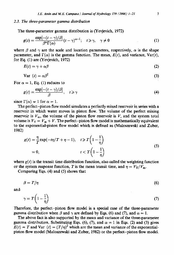
2.3. The three-parameter gamma distribution

The three-parameter gamma distribution is (Yevjevich, 1972)

e x p [ - ( t - 7)//3] ( t - 7)a-l; t>~ g(t) = ~ - - ~ 7, 7 ~ 0 (1)

where/3 and 7 are the scale and location parameters, respectively, a is the shape parameter, and F(a) is the gamma function. The mean, E(t) , and variance, Var(t), for Eq. (1) are (Yevjevich, 1972)

E(t) = 7 + a/3 (2)

Var (t) = c~/32 (3)

For a = 1, Eq. (1) reduces to

g(t) = exp[-( t - 7)//3] t/> 7 (4) /3

since F(a) = 1 for a = 1. The perfect-piston flow model simulates a perfectly mixed reservoir in series with a

reservoir in which water moves in piston flow. The volume of the perfect mixing reservoir is Vm, the volume of the piston flow reservoir is V, and the system total volume is V T = Vm + V. The perfect-piston flow model is mathematically equivalent to the exponential-piston flow model which is defined as (Maloszewski and Zuber, 1982)

g(t) = T e x p ( - t ~ 7 / T + r 1 - 1), t~> T(1-~)

t< T(1-~) (5)

where g(t) is the transit time distribution function, also called the weighting function or the system response function, T is the mean transit time, and ~ = VT/I 'm.

Comparing Eqs. (4) and (5) shows that

= r / , 7 (6)

and

Therefore, the perfect-piston flow model is a special case of the three-parameter gamma distribution when/3 and 7 are defined by Eqs. (6) and (7), and a = 1.

The above fact is also supported by the mean and variance of the three-parameter gamma distribution. Substituting Eqs. (6), (7), and a = 1 in Eqs. (2) and (3) gives E(t) = T and Var (t) = (T/r/) 2 which are the mean and variance of the exponential- piston flow model (Maloszewski and Zuber, 1982) or the perfect-piston flow model.


The perfect-piston flow model combines the perfect mixing model with the piston flow model. For r /= 1, the perfect-piston flow model gives the perfect mixing model, and for r / ~ o~, it reduces to the piston flow model. Substituting r /= 1 or letting ~ /~ c~ in Eqs. (6) and (7) yields/3 = T and 7 = 0 for the perfect mixing model, and /3 = 0, 7 = T for the piston flow model. In both perfect mixing and piston flow, the mean is T and the variance is T 2 for perfect mixing and 0 for piston flow (Malos- zewski and Zuber, 1982). These values can also be obtained from the mean and variance of the three-parameter gamma distribution. In other words, perfect mixing, piston flow, and the combination of perfect mixing-piston flow are all simulated by the three-parameter gamma distribution. In fact, as shown later, perfect mixing, partial mixing, piston flow, and their combinations (which represent reservoirs in series of the different mixing types) are all accounted for by the three-parameter gamma distribution. For this reason, we propose the general model, which takes the functional form of the three-parameter gamma distribution, for simulating mean transit times in hydrologic systems.

3. The proposed models

3.1. T i m e - i n v a r i a n t case

In this case, the general model is given by Eq. (1), where parameters a, 3, and 7 are defined as follows (derivations of the parameters can be requested from the senior author)

1 a = l ~ + # ( 1 ) ' # ~ > 0 5 1 - (8a)

1 a = l ( 1 ) ' # 4 0 . 5 (8b)

~ + (1 - # ) 1 -

(9)

m 7 = T ( 1 - ~ # + ; ) (10)

8 = VT (l l) Vm+ V

VT (12) 7 /=0V m

The general model corresponds to the general case in which lit = Vm + Vpm + V.


The variance in this case is obtained by substituting Eqs. (8) and (9) in Eq. (3). The six models which can be obtained as special cases from the general model are given in Table 1.

The first three cases in Table i correspond to the existing models of perfect-piston flow, perfect mixing, and piston flow, respectively. At the present time, there are no models to account for cases 4 and 5 which are more likely to occur in natural systems than piston flow, perfect mixing, or the combination of perfect-piston flow; and case 6 is currently modeled differently by discrete-state compartment models or the dispersive model, as indicated earlier. In this study, the models corresponding to cases 4, 5, and 6 are designated as the partial-piston flow model, perfect-partial mixing model, and partial mixing model, respectively. Note that these three models and the general model can give other models, as special cases, by changing the types of mixing or the mixing efficiency. As an example of changing the mixing efficiency, consider the perfect-partial mixing model. If # is changed from 0 < # < 1 to 0, then the perfect-partial model will give the perfect-piston flow model; if # is changed to 1, then the resulting model will be the perfect mixing model. As an example of changing the mixing type, again consider the perfect-partial mixing model. Suppose the mixing type is changed from perfect-partial mixing to just perfect mixing; then the perfect- partial mixing model will give the perfect mixing model.

3.2. Time-variant case

Following the approach of Zuber (1986b), who assumes constant parameters, the parameters in this case can be defined as

VT(t ) 1 a = V ( t ) + V m ( t ) + # V p m ( t ) = l /, i ~ = constant, #~>0.5 (13)

1 -

VT(t ) 1 C ~ = V ( t ) - t - V m ( t ) + ( 1 - # ) V p m ( t ) = l ~ + ( 1 - # ) ( 1 ) = c ° n s t a n t ' l -

# 4 0 . 5 (14)

- - + # - fl=oL

(15)

7 = 1 - - ~ - # +

where

(16)

V.r(t) 0 = V(t) + Vm(t) = constant (17)

8 LE. Amin and M.E. Campana / Journal o f Hydrology 179 (1996) 1-21

Table 1 The six models and the constant tracer input relationships

Model V T 0 r/ a Time-invariant case

Perfect-piston v. + V 1 1 g(t) = ~ e x p ( - t r l / T + rl - 1), flow

a [

- 0 , t < T ( 1 - ~ )

e x p ( - t / T ) Perfect mixing Vm 1 1 1 g(t) = T

Piston flow V 1 o¢ 1 g(t) = 6 ( t - T)

Partial-piston Vpm q- V flow

Perfect-partial Vm + Vpm mixing

Partial mixing Vpm

=0,

I /~ ~'

x exp r T ~ - -- - ~ '

t ~> T(1 1

=0,

t/> T(1 - #)

=0 , t < T(1 - / z )

I.E. Amin and M.E. Campana / Journal of Hydrology 179 (1996) 1-21 9

Time-variant case Co,~t/Cit,

CI(Z ) = r/exp[r/(1 - Z) - 1],

~o ~<(, ~)

c~ (z) = exp(-z )

C , ( Z ) = ~(1 - z )

z~0~) ox~[ ~(1 ~)]

[~+,]

1 I + A T

exp( -~T)

[~-0-~+~)] o-'

~ex~ i~(~--~/] z~> ~+~)

( ") = 0 , Z < 1 - / ~ + ~

[~_(,_~ .~°, : - ~ + ~ ) J

x exp 7]- - ~ ,

Z ~ > ( 1 1 -~-..-;) 1 -_o ~ ( , ~ .+_~)

e x p [ - A T ( 1 - # + ~ ) ]

exp (-AT(1 1 ~ "+~)]

tz - (1~ ~)1 °-' e~p~-tZ - (1 - ~)l}

Z >~(1 - # )

=o , z < ( 1 - ~ )

exp[-,~T(1 - #)]

10 LE. Amin and M.E. Campana / Journal of Hydrology 179 (1996) 1-21

Table 1 (continued)

Model V T 0 r/ a Time-invariant case

CI(Z) for the general model

Vx( t) _ constant (18) ,7 - O V m ( t )

# = constant (19)

and the weighting function for the general case VT(t) = Vm(t) + Vpm(t) + V(t), expressed as the normalized concentration response function Cz(Z ) (CI(Z) is expressed in dimensionless time, Z, the actual time divided by the mean transit time), is given in Table 1.

The six models discussed in the time-invariant section are similarly accounted for by the general G ( Z ) expression as special cases. For example, in the case of the perfect mixing model the G ( Z ) = exp( -Z) which is the same as that obtained by Niemi (1977) and Zuber (1986b). The CI(Z) functions for the six models are also given in Table I.

4. Discussion

An important feature of the models (weighting functions) obtained in this study deserves some attention. The weighting functions can assume any shape, depending on the value of ~, the shape factor. In this regard, the models developed in this study are comparable to the dispersive model and superior to any other current lumped parameter model. It is obvious that the flexibility of the weighting functions is very important if a realistic model is desired to describe the complex behavior of natural systems.

For time-invariant systems, the minimum number of fitting parameters required to model the combinations of perfect-partial mixing or partial-piston flow is three: the mean transit time (T), the mixing efficiency (#), and 0 which relates the various mixing volumes in the system. Therefore, it is not possible to account for such mixing combinations with fewer than three parameters. At the same time, using more than three parameters is unnecessary since these combinations can be completely described by three parameters. On the other hand, the minimum number of parameters required


Time-variant c a s e G o u t / G i l I

Z - (1 1

1 --#+0 Z>~ 1 - ~

to model the general case is four. These are: T, #, and two other parameters, 0 and 7, which interrelate Vm, Vpm, and V.

Grabczak et al. (1984) reported that, in practice, whenever the number of fitting parameters is larger than two, the inverse problem cannot be solved unambiguously. Such a statement cannot be generalized to include the combinations explained above. The statement is certainly true for cases in which the minimum number of fitting parameters required is less than or equal to two, which is the case for the current lumped parameter models used in tracer hydrology with the exception of discrete- state compartment models. However, one parameter models are too simplistic to describe the complex behavior of natural systems. Maloszewski and Zuber (1982), Grabczak et al. (1982), and Zuber (1986a) reported that sometimes it is impossible to obtain a good fit without introducing an additional fitting parameter under the assumption that there are at least two water components, one with the radioisotope (tracer) of interest, and another, older, component in which this radioisotope has decayed to a level beneath detection limits.

Two comments are necessary here. First, a poor fit is not necessarily due to the presence of two water components; it could as well be due to the fact that the selected model simply does not adequately describe the modeled system. Therefore, if the presence of two water components is not physically justified then the additional fitting parameter will have no physical meaning and its use will be merely to obtain a good fit even if the selected model is a one-parameter model, in which case the number of fitting parameters will be two. Second, if the appropriate model to be used is a two- parameter model, then the number of fitting parameters will exceed two. Therefore, more than two fitting parameters are needed even with the current lumped parameter models. The literature also shows that such a need is realized. Eriksson (1985) reported that some unpublished data on river water tritium in Scandinavia indicates that at most, only a three parameter model of the transit time distribution can be used with any confidence. The above discussion also applies to nonsteady state systems, in which case the number of parameters will increase because instead of the constant T (in the steady state), there are two fitting parameters, Q(t) and VT(t).

12 I.E..4rain and M.E. Campana / Journal of Hydrology 179 (1996) 1-21

v t:n

(a)

0.14

0.12

0.10

0.08

0.06

0.04

0.02

0,00

1

~ 2

4 f " ~ "

r I I

' i I , I I I I I I l

2 4 6 8 10 12 14

t ( t ime)

v o)

1 . 7 5 -

1.50 -

1 . 2 5 -

1.00

0.75

0.50

0.25

0.00

0

I

~ 2

-- -- 3

P

I I I I I

6 8 10 12 14

(b) t Olme)


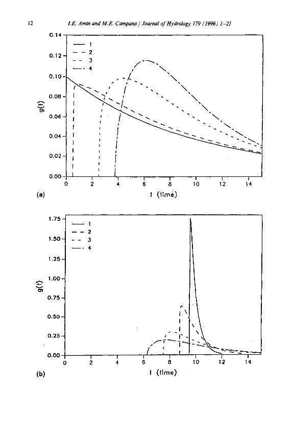
Figs. 1 (a) and (b) are graphs for weighting functions of different shapes constructed for two of the models developed in this study (the perfect-partial mixing model and the partial-piston flow model). Some of these graphs show how one model approaches another as the value of the parameters change. For example, Fig. l(a) shows that the graph with I'm = 0.9 V,r (90% of the system is perfectly mixed), closely approximates that of the perfect mixing model. Inspection of Fig. l(b) shows that as the volume occupied by piston flow increases, the variances of the graphs decrease and their peaks increase, i.e. the graphs approach piston flow since increasing V and decreasing # imply piston flow.

The most important finding of this study is the development of one model (the general model), with one set of parameters to account for the three mixing types (perfect, partial, and piston) and their combinations. In the current practice of tracer hydrology, the analytical models used to describe the three mixing types and the combination of perfect-piston flow, which is the only modeled combination at the present time, cannot be obtained as special cases from one general model. For example, the dispersive model, the Poisson distribution which describes a cascade of perfectly mixed cells used in discrete-state compartment models, and the perfect-piston flow model employ parameters of different physical meaning, and as such cannot be obtained as special cases from one general model. Our proposed model represents a unified modeling approach for the mentioned mixing types and their combinations.

4.1. The special case o f constant tracer concentration in time-invariant systems

In the case of time-invariant systems with constant tracer input, the tracer output concentration can be determined analytically using the convolution integral and the appropriate model (weighting function) that best suits the investigated system. For time-invariant systems, the convolution integral is (Zuber, 1986a)

Cout( t ) = [ C i n ( t - t ' )exp(-)~t ' )g(t ' )dt ' (20a )

0

o r

l

Cout( t ) ---- [ C i n ( t ' ) e x p [ - A ( t - t ' ) ]g ( t - t')dt' (20b)

--OQ

where Cout(t ) is the output concentration; Cin(t ) is the input concentration; exp(-At') is the factor to correct for decay if a radiotracer is used; A is the radioactive decay constant; and g(t') is the weighting function.

Fig. 1. (a) Plot of the weighting function vs. time for the perfect-partial mixing model./z = 0.50 for curves 2, 3, and 4; 1, perfect mixing model; 2, V m = 0.90VT, Vpm = 0.10Vx; 3, V m = 0.50VT, Vpm = 0.50VT; 4, Vm = 0.25VT, Vpm = 0.75VT. (b) Plot of the weighting function versus time for the partial-piston flow model. # = 0.50 for all cases; 1, V = 0.90Vr, Vpm - 0.10VT; 2, V = 0.75VT, Vpm = 0.25 VT; 3, V = 0.50VT, Vpm ~--- 0.50VT; 4, V ----- 0 .25VT, Vpm = 0 . 7 5 V T.


In Eq. (20a), t is the calendar time and t' is the integration variable which represents the transit time of water. In Eq. (20b), t' is the time of entry, t is the time of exit and (t - t') is the transit time.

Analytical determination of the mean transit time in the case of constant tracer input requires no additional information if the selected model is a one-parameter model, such as a piston flow or perfect mixing model. For two- or more parameter models, prior knowledge of the parameters other than the mean transit time, the unknown, is necessary. In practice, however, a priori knowledge of these parameters is very difficult.

The case of constant tracer input applies to the environmental radioisotopes tritium (3H), 14C, 39Ar, SSKr, and 32Si in the prethermonuclear era (Nir and Lewis, 1975; Maloszewski and Zuber, 1982) when they were produced by natural processes at practically constant levels.

Using Eq. (1) in Eq. (20a) gives

Gou t = exp(-AT) (21) Gn (A/3 + 1)

Substituting the values of~,/3, and 7 of any of the seven models into Eq. (21) gives the Gout/Gin of that particular model. For example, in the case of the general model (V T : V m "q- Vpm q- V)

Cou t 1 [ ( 1 _~)] ci=r r(± ]~exp -AT 1-~-#+ (22, [ a \r/0 + / z - +1

Knowledge of Gout, Gin, A (A = In 2/ t l /2 where tl/2 is the radiotracer half-life), and the other parameters in Eq. (22), allows the determination of T. The values of 1/A for tritium (half-life is 12.26 years) and 14C (half-life is 5730 years), two commonly used radiotracers, are 17.7 years and 8270 years, respectively.

The relationships for the other six models are given in Table 1. Note that the relationship for the partial mixing model reduces to those of the perfect mixing model for # = 1 and a = 1 and the piston flow model for # = 0 and a = 1.

5. Model application

The current literature has some guidelines for the interpretation of tracer data in clearly understood hydrologic systems. These are given below.

(1) Samples collected from springs generally represent good (perfect) mixing, because flow lines tend to converge toward springs. This is especially true for karst springs, and generally holds true for unconfined aquifers as well (Dincer and Davis, 1984).

(2) The perfect mixing model is a fair description of not-too-deep surface water bodies (Kaufman and Libby, 1954).

(3) The exponential (perfect mixing) model applies to unconfined aquifers with


shallow sampling points (flowlines with infinitesimal short transit times). Unconfined aquifers with deep sampling points should be interpreted with the dispersive or exponential (perfect)-piston flow model (Zuber, 1986a).

(4) The exponential (perfect)-piston flow model is applicable to aquifers unconfined in the upstream part and confined in the downstream part. In this case, the unconfined portion will be simulated by the exponential or perfect mixing component of the model, and the confined portion will be approximated by the piston flow component (Zuber, 1986a).

(5) Confined aquifers with a narrow recharge area far from the sampling points (width of the recharge zone is negligible in comparison with the distance to the sampling points) can be interpreted by the piston flow model or the dispersive model (Zuber, 1986a).

Based on the above guidelines, and realizing that no two hydrologic systems are alike, the following generalizations can be made for the applicability of the proposed models. Systems that tend to be highly mixed such as those in categories 1, 2, and 3 listed above can be modeled with the partial mixing model with a high mixing efficiency (i.e. the modeler has to specify a high value for #), or the perfect-partial mixing model with high/~ and/or high Vm, or the general model with high # and/or high Vm. On the other hand, systems characterized by a low degree of mixing, e.g. those in category 5, can be simulated by the partial mixing model with a low #, or the partial- piston flow model with low # and/or high V, or the general model with low # and/or high V. Category 4 systems can be analyzed with the perfect-partial mixing model, the partial-piston flow model, or the general model. Note that in case of the general model, the partially mixed volume (Vpm) will provide a realistic transitional mixing zone between the highly or perfectly mixed volume (Vm) and the piston flow volume (v).

We will give three examples to illustrate the application of the proposed models for the case of variable tracer input. The examples are limited to systems in the steady state since few data exist for transient flow systems.

In the first two examples, data obtained by Davis et all (1970) from two springs (site 45 and site 2) on Cheju Island, Republic of Korea, are reinterpreted.

Davis et al. (1970) summarized the geology and geohydrology of Cheju Island as follows. Cheju Island is an eUiptically shaped volcanic island. It has an area of 1792 km 2 and is about 75 km long in an east-west direction and 32 km wide in a north- south direction. The rocks of Cheju are almost entirely of volcanic origin with a predominance of basalt but including some andesitic rock types. Most of the volcanic rocks are vesicular and are cut by numerous joints and fissures. Lava tunnels and scoriaceous contact zones of individual lava flows are common and provide conduits for rapid groundwater flow.

Rainfall is abundant on Cheju Island. The 30-year normal (1931-1960) for Cheju City on the north coast indicates an annual average of 1440 mm. This total is exceeded by a large amount at higher altitudes in the interior of the island. About 60% of the rainfall occurs from June through September. Despite the heavy rainfall there is little sustained streamflow on the island. Torrential runoff occurs during and immediately after rain, but the high permeability of the volcanic rocks encourages rapid infiltration.


300

250 -

2 0 0 -

1--

I ' -

1 5 0 -

I O 0 -

5 0 -

- - Por l lo l Mixin 9 Model

• Sile 45 Observo l ions

- - Por l io I -P imton Flow Model

* Sile 2 0 b s e r v o t i o n l

I

b

"e,

, _ _ _ . _ ~ , - - . . . . . ,_ . , ~ . _

O - I I I I I I I

0 1 9 6 5 1 9 6 6 1 9 6 7 1968

YEARS

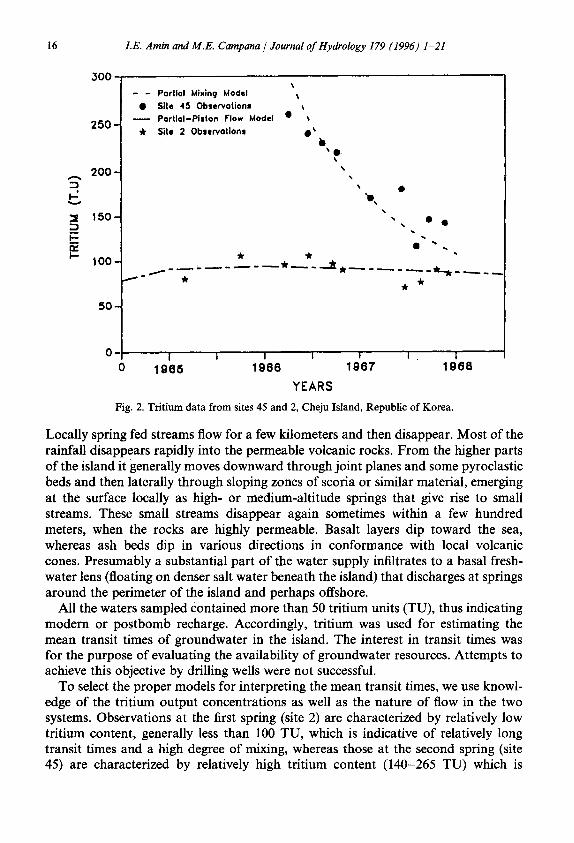
Fig. 2. Tritium data from sites 45 and 2, Cheju Island, Republic of Korea.

Locally spring fed streams flow for a few kilometers and then disappear. Most of the rainfall disappears rapidly into the permeable volcanic rocks. From the higher parts of the island it generally moves downward through joint planes and some pyroclastic beds and then laterally through sloping zones of scoria or similar material, emerging at the surface locally as high- or medium-altitude springs that give rise to small streams. These small streams disappear again sometimes within a few hundred meters, when the rocks are highly permeable. Basalt layers dip toward the sea, whereas ash beds dip in various directions in conformance with local volcanic cones. Presumably a substantial part of the water supply infiltrates to a basal fresh- water lens (floating on denser salt water beneath the island) that discharges at springs around the perimeter of the island and perhaps offshore.

All the waters sampled contained more than 50 tritium units (TU), thus indicating modern or postbomb recharge. Accordingly, tritium was used for estimating the mean transit times of groundwater in the island. The interest in transit times was for the purpose of evaluating the availability of groundwater resources. Attempts to achieve this objective by drilling wells were not successful.

To select the proper models for interpreting the mean transit times, we use knowledge of the tritium output concentrations as well as the nature of flow in the two systems. Observations at the first spring (site 2) are characterized by relatively low tritium content, generally less than 100 TU, which is indicative of relatively long transit times and a high degree of mixing, whereas those at the second spring (site 45) are characterized by relatively high tritium content (140-265 TU) which is


indicative of relatively shorter transit times and a lower degree of mixing than at site 2. On the other hand, the fact that flow is taking place in lava tunnels and fractures is suggestive of mixing that can assume any degree or efficiency depending on the fracture shape, size, orientation, and interconnection.

Based on the above information, we chose the partial mixing model with relatively short T and moderate # for the interpretation of site 45. Using this model, the best fit is obtained for T --- 2.4 years (standard deviation is 0.8 years), # = 0.5, and it is good at the 0.01 significance level as indicated by the chi-square goodness of fit test. The predicted and observed output concentrations are shown in Fig. 2. In the case of site 2, we selected the partial-piston flow model with relatively long T and high #. The best fit, significant at the 0.1 significance level, is obtained for T----21 years (standard deviation is 19.3 years), # -- 0.98, 0 -- 18.9; and it is also given in Fig. 2. Note that the value of 0 which corresponds to Vpm = 0.947 VT, and V -- 0.053 V T and the high mixing efficiency show the tendency of the system to be highly mixed. Davis et al. (1970) used the binomial model, which is a simplified form of the dispersive model, and determined T = 3 years for site 45, and T = 8.5 years for site 2. Later, Malos- zewski and Zuber 0982) reinterpreted the data from both sites with the exponential- piston flow model (which is mathematically equivalent to the perfect-piston flow model). They obtained T--2 .5 years for site 45, comparable to the value of T -- 2.4 years obtained in this study, and T ---- 21 years for site 2, the same value estimated in this study.

The third example shows the applicability of the proposed models to fiver basin studies. The example is a reinterpretation of tritium data collected from the Ottawa River basin in Canada.

Monitoring of tritium in the Ottawa River (output) and in the precipitation of the Ottawa River basin (input) began in 1953 following the inception of large-scale atmospheric thermonuclear testing in 1952. This makes it the only river system with a fairly complete record of tritium (Eriksson, 1985). The availability of these data allowed Brown (1961) to estimate the mean transit time of water in the basin. Later, Eriksson (1963) derived the transit time distribution by analyzing the data with a different approach, the so-called identification approach in systems analysis terminology.

The length of the river above the sampling point is 640 km and the drainage area is 62 000 km 2, all. of which is within the Canadian Shield. The average discharge during the period 1950-1959 was 28 260 ft 3 s -1. The bedrock geology of the basin above the sampling point consists of Precambrian granites, gneiss and other crystalline and metamorphic rocks through which water moves in fractures and joints. There is extensive rock outcrop on all slopes, but the valleys are generally wide and well filled with glacial drift providing considerable ground storage capacity. A conventional hydrological study involving analysis of local geology and permeability measurements, while yielding very detailed information, is a major undertaking for such a large area. On the other hand, correlation of the injection and the discharge of tritium in such a drainage system should give information on the mean transit time (Brown, 1961).

In this study, we determine the mean transit time of water in the system with the

18 I.E. Amin and M.E. Campana / Journal of Hydrology 179 (1996) 1-21

I-- v

I--

I--

300

250'

200 -

150

100

5 0 -

- - Perfect-Port iol Mixing Model 4P "

• O b s e r v a t i o n s i ~ ,, I •

! n I

I

I

I

I

I

/

• e . . •

I

e , I

0 I I I I I

0 1 9 5 7 1 9 5 8 1 9 5 9 1 9 6 0 1 9 6 1

YEARS

Fig. 3. Tf i t iumdata~om Ottawa ~verbas in , Can~a.

• 8

perfect-partial mixing model owing to the general tendency of such systems to be highly mixed. Fig. 3 shows the best fit obtained for T = 3 years (standard deviation is 2.6 years),/z = 0.2, and 0 = 1.1 (indicating Vm = 0.9VT, i.e. 90% of the system is perfectly mixed). In this case, the obtained fit is found to be good at the 0.5 significance level. The T values obtained by Brown (1961) and Eriksson (1963) compare very well with the one found in this study. Brown's interpretation resulted in T = 3.3 years, and that of Eriksson yielded T = 3.0 years.

6. Summary and conclusions

We have presented a general lumped parameter mathematical model capable of interpreting hydrologic tracer data and simulating a variety of mixing regimes. The general model takes the form of the three-parameter gamma distribution; special cases, depicting the mixing types of piston flow (no mixing), partial mixing, and perfect mixing can be obtained from the general model. The existing models of piston flow, perfect mixing and the perfect-piston flow (or exponential-piston flow) model can be obtained from the general model. Partial mixing can be modeled separately or in combination with perfect mixing or piston flow with the perfect-partial model and the partial-piston flow model, respectively. No current models are available for these latter two combinations. Furthermore, partial mixing is simulated free from the dispersivity limitations (scale-dependence). The shape flexibility of the weighting


functions presented in this paper are comparable to those of the dispersive model and superior to that of any current lumped parameter model. The model can also treat transient systems although such data are generally difficult to obtain.

Applications of the model to the groundwater system on Cheju Island, Republic of Korea, and the Ottawa River basin in Canada yield transit time calculations similar to those calculated by previous investigators.

In conclusion, the proposed models have the potential for estimating mean transit times in hydrologic systems characterized by different mixing regimes.

Acknowledgments

We thank the Water Resources Center, Desert Research Institute, University of Nevada Systems, and the State of Nevada's Carbonate Aquifer Studies Program for their financial support. We also thank the Department of Earth and Planetary Sciences, University of New Mexico and the Department of Geological Sciences, California State University-Long Beach, for their support. We are grateful to Mary Sherman for her word-processing skills. I. Amin thanks his wife for her inspiration and moral support.

Appendix A. List of symbols

c (z)

ci.(t) Cout(/) E(t) g(t)

a t

T Var (t) V Vm Vpm lit Z

weighting function in the non steady-state case. Ci(Z) is expressed as a function of dimensionless time Z = t iT tracer input concentration tracer output concentration mean of the three-parameter gamma distribution transit time distribution function, also called the weighting function of the system response function volumetric flow rate through the system time variable radiotracer half-life transit time variable mean transit (residence) time of water in the system variance of the three-parameter gamma distribution volume in which water moves in piston flow volume occupied by perfect mixing volume occupied by partial mixing total volume of mobile water in the system dimensionless time = t~ T

Greek letters

a, fl, 7 parameters of the three-parameter gamma distribution; a, fl, 7 are the shape, scale, and location parameters, respectively

2O

r( ) 5

0

A #


gamma function Dirac delta function VT

OVm VT

Vm+ V radioactive decay constant mixing efficiency, which equals unity for perfect mixing and zero for piston flow

References

Anderson, M.P., 1979. Using models to simulate the movement of contaminants through groundwater flow systems. CRC Crit. Rev. Environ. Control, 9(2): 97-156.

Bredehoeft, J. and Pinder, G., 1973. Mass transport in flowing groundwater. Water Resour. Res., 9: 194- 210.

Brown, R.M., 1961. Hydrology of tritium in the Ottawa Valley. Geochim. Cosmochim. Acta, 21: 199-216. Campana, M.E., 1975. Finite-state models of transport phenomena in hydrologic systems. Ph.D. Disserta-

tion, University of Arizona, Tucson, AZ. Davis, G.H., Lee, Ch.K., Bradley, E. and Payne, B.R., 1970. Geohydrologic interpretation of a volcanic

island from environmental isotopes. Water Resour. Res., 6: 99-109. Dincer, T. and Davis, G.H., 1984. Application of environmental isotope tracers to modeling in hydrology.

J. Hydrol., 68: 95-113. Eriksson, E., 1963. Atmospheric tritium as a tool for the study of certain hydrologic aspects of river basins.

TeUus, 15(3): 303-308. Eriksson, E., 1985. Principles and Applications of Hydrochemistry. Chapman and Hall, New York. Gelhar, L.W., Welty, C. and Rehfeldt, K.R., 1992. A critical review of data on field-scale dispersion in

aquifers. Water Resour. Res., 28: 1955-1974. Grabczak, J., Zuber, A., Maloszewski, P., Rozar~ski, K., Weiss, W. and Sliwka, I., 1982. New mathematical

models for the interpretation of environmental tracers in groundwaters and the combined use of tritium, C-14, Kr-85, He-3 and freon-11 methods. Beitr. Geol. Schweiz, Hydrology Service, 28(2), pp. 395-404.

Grabczak, J., Maloszewski, P., Rozanski, K. and Zubcr, A., 1984. Estimation of the tritium input function with the aid of stable isotopes. Catena, 11: 105-114.

Kaufman, S. and Libby, W.F., 1954. The natural distribution of tritium. Phys. Rev., 93: 1337-1344. Maloszewski, P. and Zuber, A., 1982. Determining the turnover time of groundwater systems with the aid

of environmental tracers, I. Models and their applicability. J. Hydrol., 57:207-231. Nash, J.E., 1957. The form of the instantaneous unit hydrograph. Publ. No. 45, IASH, pp. 114-121. Niemi, A., 1977. Residence time distributions of variable flow processes. Int. J. Appl. Radiat. Isot., 28: 855-

860. Nir, A., 1964. On the interpretation of tritium 'age' measurements of groundwater. J. Geophys. Res., 69:

2589-2595. Nit, A. and Lewis, S., 1975. On tracer theory in geophysical systems in the steady and non-steady state, Part

I. Tellus, 27: 372-382. Przewlocki, K. and Yurtsever, Y., 1974. Some conceptual mathematical models and digital simulation

approach in the use of tracers in hydrological systems. In: Isotope Techniques in Groundwater, Vol. II. IAEA, Vienna, pp. 425-450.

Simpson, E.S. and Duckstein, L., 1976. Finite-state mixing cell models. In: V. Yevjevich (Editor), Karst Hydrology and Water Resources. Water Resources, Fort Collins, CO, pp. 489-512.


Wheatcraft, S.W. and Tyler, S.W., 1988. An explanation of scale-dependent dispersivity in heterogeneous aquifers using concepts of fractal geometry. Water Resour. Res., 24(4): 566-578.

Yevjevich, V., 1972. Probability and Statistics in Hydrology. Water Resources, Fort Collins, CO. Zuber, A., 1986a. Mathematical models for the interpretation of environmental radioisotopes in ground-

water systems. In: P. Fritz and J. Ch. Fontes (Editors), Handbook of Environmental Isotope Geo- chemistry, Vol. 2. Elsevier, Amsterdam, pp. 1-60.

Zuber, A., 1986h. On the interpretation of tracer data in variable flow systems. J. Hydrol., 86: 45-57.

Documents

Hydrology - Campanastanaquadoc.typepad.com/files/campana_and_amin_1996.pdf · LE. Amin and M.E. Campana / Journal of Hydrology 179 (1996) 1-21 3 recognize that the proposed model