Embed Size (px)
Citation preview

HYDRODYNAMIC MODELLING OF LAKE ONTARIO
by
ERIN HALL
A thesis submitted to the
Department of Civil Engineering
in conformity with the requirements for
the degree of Masters of Science (Engineering)
Queen’s University
Kingston, Ontario, Canada
October 2008
Copyright c© Erin Hall, 2008

Abstract
The 2006 Clean Water Act requires each municipality to come up with science-
based plans to protect the quality and quantity of their drinking water. A litera-
ture review concerning applicable processes in Lake Ontario along with previous
modelling of the lake is presented.
The three dimensional Estuary, Lake and Coastal Oceans Model (ELCOM) is
used to model Lake Ontario on a 2 × 2 km grid scale. The model is forced using
meteorological data from the 2006 summer season, inflows and outflows. The lake-
wide model is evaluated using field data from thermistor chains and ADCPs as
well as historical water level data. Simulated and observed temperature profiles
compared well. However, modelled temperature profiles were slightly cooler than
observed. Current results were more variable than temperature profile results but
compared better to observed data in the offshore regions. Simulating Lake Ontario
water levels proved to be problematic because an accurate water balance is difficult
to force with a large drainage basin.
A 300 × 300 m nearshore model of the eastern portion of Lake Ontario and the
upper St. Lawrence River is also presented. The open boundary is forced using
temperature data which is (A) varied with depth, (B) constant with depth and (C)
spatially varied over the length of the open boundary and varied with depth. Both
i
spatially varied and non-varied water level data forcing the open boundary is also
compared. Spatially varied temperature and water level data is computed from the
coarse grid lake-wide model. Lake-wide coarse grid model error appears to prop-
agate through the open boundary negatively affecting nearshore modelled current
when coupling the models. It was concluded that lake-wide model results should
not be used to force the open boundary for the nearshore model. Nearshore model
results using constant temperature with depth forcing files and non-spatially var-
ied water level data agree well with observed temperature profiles, but further
analysis is required for better confidence in the model’s ability to properly repro-
duce currents at a 300 × 300 m grid scale.
ii

Acknowledgments
Thanks first of all to my parents, sisters, grandparents and aunts for their uncon-
ditional love and support throughout my entire education at Queen’s. A special
thanks goes to officemates Jonathan my voice of calming reason, Imran and Whit-
ney as well as all my 4th floor and other Ellis friends. Thank you to my housemates
Anne, Morgan, Jarrett, Pico and Alex who have listened to my boring, nerdy grad
student stories and rants as well as provided me with much needed distractions.
Thank you to Leon for providing me with this opportunity and to Kevin for
guiding me through this process that is called a Masters as well as giving me the
chance to practice some very important life skills not normally exercised in the
realm of a Masters through APSC 190. Thanks also go to the lovable and very
helpful civil office ladies and to Bob Rosswell and the captain of his little tin ship
at NWRI for getting me out of my little office and on the water for a day!
Thanks to all my friends who have made my time at Queens so memorable,
in particular Sarah, Valerie, Alisa and my soccer ladies. Thank you to my fellow
servers at Tango and the lovable kitchen staff who I’ve very much enjoyed working
with over the last year of my Masters.
Finally a great big thanks to Paul for pulling me through these very difficult last
few months even from the other side of the world and giving me the best ”almost
iii

submitted” present ever!
iv

This thesis is dedicated to Lyn, who taught me how to find the value in all of
life’s experiences.
v

Table of Contents
Abstract i
Acknowledgments iii
Table of Contents vi
List of Tables viii
List of Figures ix
Chapter 1:Introduction . . . . . . . . . . . . . . . . . . . . . . . . . . . . . . 1
1.1 The Relationship Between the Great Lakes and Society . . . . . . . . 11.2 The Need for Hydrodynamic Modelling for Water Quality . . . . . . 21.3 Other Benefits of Lake Modelling for Scientific Advancement . . . . . 41.4 Study Objectives and Outline . . . . . . . . . . . . . . . . . . . . . . . 5
Chapter 2:Literature Review . . . . . . . . . . . . . . . . . . . . . . . . . . . 7
2.1 Review of Physical Processes in Large Lakes . . . . . . . . . . . . . . 72.2 ELCOM . . . . . . . . . . . . . . . . . . . . . . . . . . . . . . . . . . . . 24
Chapter 3:Lake Ontario Basin Scale Hydrodynamics Model . . . . . . . . 30
3.1 Introduction . . . . . . . . . . . . . . . . . . . . . . . . . . . . . . . . . 303.2 Methods and Materials . . . . . . . . . . . . . . . . . . . . . . . . . . . 333.3 Results . . . . . . . . . . . . . . . . . . . . . . . . . . . . . . . . . . . . 423.4 Discussion . . . . . . . . . . . . . . . . . . . . . . . . . . . . . . . . . . 563.5 Conclusion . . . . . . . . . . . . . . . . . . . . . . . . . . . . . . . . . . 65
Chapter 4:Nearshore Hydrodynamic Model . . . . . . . . . . . . . . . . . . 68
vi

4.1 Introduction . . . . . . . . . . . . . . . . . . . . . . . . . . . . . . . . . 684.2 Model Description and Data . . . . . . . . . . . . . . . . . . . . . . . . 704.3 Results . . . . . . . . . . . . . . . . . . . . . . . . . . . . . . . . . . . . 774.4 Discussion . . . . . . . . . . . . . . . . . . . . . . . . . . . . . . . . . . 934.5 Conclusion . . . . . . . . . . . . . . . . . . . . . . . . . . . . . . . . . . 96
Chapter 5:Conclusions . . . . . . . . . . . . . . . . . . . . . . . . . . . . . . 99
5.1 Lake-Wide ELCOM Results . . . . . . . . . . . . . . . . . . . . . . . . 995.2 Nearshore ELCOM Results . . . . . . . . . . . . . . . . . . . . . . . . . 1025.3 Future Work . . . . . . . . . . . . . . . . . . . . . . . . . . . . . . . . . 103
Bibliography . . . . . . . . . . . . . . . . . . . . . . . . . . . . . . . . . . . . . 105
Appendix A:Scaled vs Non-Scaled Temperature Profiles . . . . . . . . . . 111
Appendix B:Water Levels . . . . . . . . . . . . . . . . . . . . . . . . . . . . . 116
Appendix C:Lake-Wide Current Comparisons . . . . . . . . . . . . . . . . 121
Appendix D:ELCOM Transport Equations . . . . . . . . . . . . . . . . . . . 127
Appendix E:Velocity Difference . . . . . . . . . . . . . . . . . . . . . . . . . 130
vii

List of Tables
3.1 Data acquisition buoys in Lake Ontario . . . . . . . . . . . . . . . . . 40
4.1 Depth averaged RMS analysis results for temperature profiles . . . . 824.2 RMS analysis results for current profiles . . . . . . . . . . . . . . . . . 92
B.1 Modelled monthly tributary flow data obtained from NOAA . . . . . 117
viii

List of Figures
2.1 Langmuir circulation . . . . . . . . . . . . . . . . . . . . . . . . . . . . 15
3.1 Wind direction, wind temperature and air temperature data . . . . . 373.2 Short and longwave radiation, atmospheric pressure and relative
humidity data . . . . . . . . . . . . . . . . . . . . . . . . . . . . . . . . 383.3 Inflow, outflow, tributary and rain data . . . . . . . . . . . . . . . . . . 393.4 Lake Ontario bathymetry . . . . . . . . . . . . . . . . . . . . . . . . . . 403.5 Modelled and observed temperature at station 1263 . . . . . . . . . . 443.6 Modelled and observed temperature at station 586 . . . . . . . . . . . 453.7 Modelled and observed temperature at station 403 . . . . . . . . . . . 473.8 Modelled and observed temperature at station 1266 . . . . . . . . . . 483.9 Water level fluctuations including major inflows, outflows and pre-
cipitation . . . . . . . . . . . . . . . . . . . . . . . . . . . . . . . . . . . 503.10 Water level fluctuations including tributary flow, precipitation and
major inflows and outflow . . . . . . . . . . . . . . . . . . . . . . . . . 513.11 Modelled and observed velocity comparisons at station 1266 . . . . . 533.12 Modelled and observed velocity comparisons at station 1263 . . . . . 553.13 Scaled modelled and observed water level fluctuations . . . . . . . . 603.14 ELCOM bathymetry compared to observed bathymetry at stations
1263 and 1266 . . . . . . . . . . . . . . . . . . . . . . . . . . . . . . . . 623.15 Beletsky et al.’s plot of summer circulation . . . . . . . . . . . . . . . . 643.16 Lake-wide ELCOM mean circulation . . . . . . . . . . . . . . . . . . . 65
4.1 Wind direction, wind temperature, air temperature and relative hu-midity data . . . . . . . . . . . . . . . . . . . . . . . . . . . . . . . . . . 73
4.2 Short- and longwave ratidation, atmospheric pressure and rain data . 744.3 Map of the modelled area showing station locations . . . . . . . . . . 754.4 Gridded ELCOM nearshore bathymetry . . . . . . . . . . . . . . . . . 764.5 ELCOM temperature comparison at station 1262 for simulations A,
B and C . . . . . . . . . . . . . . . . . . . . . . . . . . . . . . . . . . . . 784.6 ELCOM temperature comparison at station 1263 for simulations A,
B and C . . . . . . . . . . . . . . . . . . . . . . . . . . . . . . . . . . . . 79
ix
4.7 ELCOM temperature comparison at station 1264 for simulations A,B and C . . . . . . . . . . . . . . . . . . . . . . . . . . . . . . . . . . . . 80
4.8 ELCOM temperature comparison at station 1265 for simulations A,B and C . . . . . . . . . . . . . . . . . . . . . . . . . . . . . . . . . . . . 81
4.9 RMS current analysis at station 1262 for simulations A, B and C . . . 834.10 RMS current analysis at station 1263 for simulations A, B and C . . . 844.11 RMS current analysis at station 1264 for simulations A, B and C . . . 854.12 RMS current analysis at station 1265 for simulations A, B and C . . . 864.13 ELCOM current comparison at station 1262 . . . . . . . . . . . . . . . 884.14 ELCOM east component of velocity comparison at station 1263 . . . 894.15 ELCOM north component of velocity comparison at station 1263 . . . 904.16 RMS analysis for currents at station 1263 for simulations A, B and C . 92
A.1 Scaled vs unscaled temperature profile comparisons at station 1263 . 112A.2 Scaled vs unscaled temperature profile comparisons at station 586 . . 113A.3 Scaled vs unscaled temperature profile comparisons at station 403 . . 114A.4 Scaled vs unscaled temperature profile comparisons at station 1266 . 115
B.1 Water level comparison for a closed basin . . . . . . . . . . . . . . . . 118B.2 Water level comparison for a simulation including major inflows
and outflow . . . . . . . . . . . . . . . . . . . . . . . . . . . . . . . . . 119B.3 Water level comparison for a simulation including major inflows,
outflow and precipitation . . . . . . . . . . . . . . . . . . . . . . . . . 120
C.1 Lake-wide ELCOM simulated summer depth averaged mean circu-lation . . . . . . . . . . . . . . . . . . . . . . . . . . . . . . . . . . . . . 122
C.2 Lake-wide ELCOM simulated summer season surface circulation . . 123C.3 Lake-wide ELCOM simulated surface currents for August 2006 . . . 124C.4 Lake-wide ELCOM simulated surface currents for May 2006 . . . . . 125C.5 Lake-wide ELCOM simulated currents at a depth of 3.5 m . . . . . . 126
D.1 ELCOM equations . . . . . . . . . . . . . . . . . . . . . . . . . . . . . . 128D.2 ELCOM nomenclature . . . . . . . . . . . . . . . . . . . . . . . . . . . 129
E.1 Coarse grid model velocity difference at station 1263 . . . . . . . . . . 132E.2 Coarse grid model velocity difference at station 1266 . . . . . . . . . . 133E.3 Nearshore model north component of velocity difference at station
1263 . . . . . . . . . . . . . . . . . . . . . . . . . . . . . . . . . . . . . . 134E.4 Nearshore model east component of velocity difference at station 1263135
x

Chapter 1
Introduction
1.1 The Relationship Between the Great Lakes and So-
ciety
The Great Lakes serve many functions including providing source drinking wa-
ter and a sink for pollutants and runoff [1] as well as a source of recreation for
many urban areas surrounding them. Circulation in the Great Lakes has been of
interest since the late 19th century for a variety of applications such as transporta-
tion, fishing, agriculture, waste disposal and now source water. Most recently, due
to the Clean Water Act passed in October 2006 by the Ontario government, the
responsibility of drinking water protection has been placed in the hands of each
municipality.
Considerable interest has now evolved in determining new alternatives for pro-
viding safe drinking water to communities [1]. These new alternatives include,
1
CHAPTER 1. INTRODUCTION 2
identification of potential sources of contamination and the creation and imple-
mentation of a plan to protect the quality and quantity of drinking water. The
coastal zones of large lakes are the areas of most immediate concern to the general
public because circulation and mixing in the nearshore region is very important for
the loading, pathways and fate of pollutants in lakes and for locating water intakes
and waste water treatment plants [2]. These zones are areas of intense biological,
chemical and geological processing of materials arriving from both on and offshore
zones [3] and the currents associated with the nearshore are especially important
for understanding the dispersal of pollutants and waste heat in the lakes as well as
recreational usage [4].
Modelling of lake hydrodynamics also plays a large role in tracking and better
understanding algal blooms which affects water quality [5, 6]. The proper rep-
resentation of temperature stratification is of particular significance in regulating
vertical transport of nutrients, plankton and oxygen, enabling a better understand-
ing of the occurrence of of hypolimnetic anoxia [7].
1.2 The Need for Hydrodynamic Modelling for Water
Quality
Increasing concern with source water quality has stimulated interest in the study
of numerical models as a tool for understanding the relevant processes in a source
water body with the purpose of predicting the effect of changing conditions and
to simulate the input and dispersion of contaminants [6]. It is important to un-
derstand the physical processes and mean circulation patterns in the Great Lakes

CHAPTER 1. INTRODUCTION 3
for ecological management issues as they provides an indication of transport path-
ways of nutrients and contaminants [8, 9].
For many environmental problems in the Great Lakes, it is necessary to know
the time-dependent, three-dimensional temperature distribution and circulation
which is frequently dominated by wind-induced upwellings and coastally trapped
waves [10]. Being able to capture the physics of internal waves is also considered
valuable as internal waves break along sloping boundaries and distribute their
momentum and energy which impacts mixing across the pycnocline, sediment re-
suspension, and the distribution of both phytoplankton and nutrients in the water
column which influences the biogeochemical systems in a lake [11, 12]. Therefore,
hydrodynamic modelling is the appropriate transport foundation for an accurate
lake mass balance model because it offers a basis for simulating transport in re-
sponse to meteorological forcing functions and its results can be scaled to the de-
sired spatial and temporal resolution [6]. The air/water interface and its processes
such as wind and waves, are important phenomena to understand because this
is where the exchange of the physical quantities such as heat, kinetic energy, mo-
mentum, and matter (gases, vapor, aerosols, etc.) occurs [13]. Accurate forcing
data is essential for these models. However, basin-scale internal waves provide
the driving forces for vertical and horizontal fluxes in a stratified lake below the
mixed layer therefore modelling the basin-scale internal wave behaviour is a priori
requirement to modelling and quantifying the flux paths of nutrients in a stratified
lake [14].
Studies have shown that there is significant value in performing comprehensive
three-dimensional simulations to evaluate possible pollutant concentration levels

CHAPTER 1. INTRODUCTION 4
to protect source water [1]. The flow patterns in hundreds of lakes and reservoirs
around the world have been modelled with the goal of protecting source water,
some of these include Lake Kinneret in Isreal [14], Lake Biwa in Japan [15] and the
Great Lakes in North America [1, 6, 16].
1.3 Other Benefits of Lake Modelling for Scientific Ad-
vancement
Large enclosed and rotating basins like the Great Lakes are subjected to many of
the same forcings as coastal oceans and can serve as examples for understand-
ing the more complicated coastal ocean dynamics [3]. Lakes are easier to study
than coastal ocean zones because they are not subjected to salinity effects or tides
and open boundary conditions are not required [10]. The size of the Great Lakes
also makes them of interest to hydrodynamic modellers because the effects of the
Earth’s rotation are important to their dynamics but they are not large enough for
the curvature effects of the Earth’s surface to be of significance. Furthermore, vari-
ations of the Coriolis parameter are negligible but lateral boundaries cannot be
ignored [9]. These boundaries can, however, emphasize wave-induced complexi-
ties for lakes, reservoirs, and estuarine waters compared to in the open ocean [13].
A better understanding of these processes will provide a better prediction in both
the lake and ocean environments [10].

CHAPTER 1. INTRODUCTION 5
1.4 Study Objectives and Outline
The objective the Intake Protection Zone (IPZ) study initiated by the CRCA is to
first delineate drinking water intake protection zones and then produce an inven-
tory and map of all threats and issues in those zones. The first stage in water
quality tracking is understanding circulation which in this case necessitates the
construction of an accurate flow model. Three dimensional hydrodynamic mod-
elling is an appropriate tool for understanding the relevant processes in a source
water body to simulate the changing conditions which may affect the quality of
drinking water [6]. The objectives of this thesis project is to first test a course 2 ×
2 km model of Lake Ontario and evaluate its performance in the near and offshore
regions by comparing its results to observed temperature, current and water level
data. Secondly, the Kingston basin and the upper portion of the St. Lawrence river
are modelled on a finer 300 × 300 m grid scale with an open boundary with the
goal of evaluating the sensitivity of the open boundary and how well the model
performs at this grid scale in the nearshore areas in terms of temperature and cur-
rents.
Chapter 2 presents a literature review which discusses physical processes ap-
plicable to circulation of large lakes and introduces the three dimensional hydro-
dynamics model used to simulate the circulation in Lake Ontario in Chapters 3
and 4. Modelling limitations are also discussed and two examples of the model’s
previous use are detailed.
Chapter 3 presents a coarse grid lake-wide three dimensional hydrodynamic
model of Lake Ontario. The model is evaluated using thermistor chain, histori-
cal water levels and ADCP data. Lake-wide circulation results are also compared

CHAPTER 1. INTRODUCTION 6
to Lake Ontario circulation patterns from literature. The goal is to evaluate the
model’s ability to reproduce general circulation patterns in the near and offshore
regions.
Chapter 4 provides a description of a nearshore fine grid model of the Kingston
basin and the upper portion of the St. Lawrence River. Three simulations using an
open boundary forced by temperature and water level data are compared. Result-
ing temperature profiles and currents are compared to thermistor chain, ADCP
and current meter data with the goal of evaluating how well general circulation
patterns are reproduced by the model on a fine grid scale in the nearshore areas.
Lastly, Chapter 5 summarizes the findings from the lake-wide and nearshore
models presented in Chapters 3 and 4.

Chapter 2
Literature Review
2.1 Review of Physical Processes in Large Lakes
2.1.1 Introduction
Circulation in the Great Lakes is driven primarily by wind stress and surface heat
fluxes. The combination of these two factors coupled with the lake’s unique bathymetry
makes circulation patterns in large lakes rather complex [8, 9]. Density currents
also play a part in forming the driving energy fluxes in a large stratified lake [14].
The energy flux from the wind is of particular interest because of its dominant
role in setting the thermocline in motion, which, in the absence of inflows and out-
flows, is the primary energy store for transport and mixing below the wind-mixed
layer [14, 17]. Many other physical processes are either initiated by or associated
with wind and must be considered to properly understand the physical processes
which drive water movement in large lakes. Wind stress induces seiches, differ-
ent types of internal waves such as Poincare waves, Kelvin waves, coastal jets and
7

CHAPTER 2. LITERATURE REVIEW 8
more. Temperature is the other main contribution to circulation. The Great Lakes
are considered dimictic lakes and therefore have a period of thermal stratification
and a period of almost uniform water temperature throughout the lake’s water
column. Temperature stratification plays a large role in the development of circu-
lation in large lakes at mid latitudes like the Great Lakes.
2.1.2 Thermal Stratification
In Lake Ontario, summer circulation is characterized by thermal stratification [17].
Thermal stratification usually occurs in late May or early June and lasts through
October [4, 8]. During stratification, the lake is characterized by an upper layer of
more or less uniformly warm, circulating and sometimes turbulent water called
the epilimnion. The thermocline separates the upper warm waters from the colder
and denser bottom layer of the lake, the hypolimnion, and is the plane of maxi-
mum rate of decrease of temperature with respect to depth [18]. If it is a windy
spring, the thermocline will setup lower and gradually rise as further heating oc-
curs. If there are light winds at the time of thermocline onset, stratification will
setup higher and progressively descend as wind-induced mixing establishes the
epilimnion. After setup, the depth of the thermocline will deepen as the upper
layer gains small amounts of heat throughout the period of stratification [18]. Dur-
ing the summer, when the daily heat input exceeds the nighttime loss, the thermo-
cline will strengthen and deepen. In the fall, nighttime cooling exceeds daytime
heating and the stratification is eroded.
At the onset of stratification, a thermal bar occurs. There is an inclined ther-
mocline separating warmer water in the nearshore band from the still barotropic

CHAPTER 2. LITERATURE REVIEW 9
cooler waters in the middle of the lake. As time progresses, the volume of warm
water increases and the thermocline becomes stronger and moves further out from
shore [4] and eventually establishes thermal stratification throughout the entire
lake.
Although the greatest source of heat to lakes is solar radiation, the direct ab-
sorption of solar radiation accounts for only about 10% of the observed distribu-
tion of heat. Most of the heat distribution profile results from circulation caused
by wind stress [18]. Significant motion is confined to the warmer layers above
the thermocline [4]. The transport of heat by turbulence decreases as the stabil-
ity of stratification increases throughout the summer months and the heat flux
in the hypolimnion varies minimally with increasing depth [18]. The stable and
rapid change in water density at the thermocline acts as a semi-permeable barrier
which can dissipate basin-scale energy from basin-scale waves via turbulent mix-
ing through shear instabilities as would a lake boundary such as the lake floor in
the absence of thermal stratification [19]. This type of internal turbulence accounts
for approximately 10% of the decay of internal wave energy whereas internal wave
energy dissipation at the lake perimeter accounts for about 90%. Thermoclines
can also support internal gravity waves generated by atmospheric pressure fluc-
tuations, wind, buoyancy flux, interaction of basin-scale motion with bottom to-
pography, instabilities in the mean currents and non-linear wave-wave interaction
[15].
A difference of only a few degrees is sufficient to prevent circulation of water
between the hypolimnion and the epilimnion [18]. Because of the density barrier
created by the steep temperature gradient of the thermocline, the hypolimnion can

CHAPTER 2. LITERATURE REVIEW 10
move in a different direction from the epilimnion. In the deeper offshore regions,
the pressure gradient (caused by the surface water level gradient) can generate
transport opposite to the wind direction [8]. This was also seen in studies con-
ducted by Bennett [20].
Wind-induced transport of heat is usually of greater importance than direct
solar heating in most lakes, especially where light is rapidly attenuated with in-
creasing depth as it is in Lake Ontario [18]. Wind stress applied to a stratified lake
forms a turbulent surface mixing layer. Turbulence distributes wind momentum
and heat through the depth of the water layer, therefore the epilimnion moves
downwind [19]. Continued application of wind stress to a stratified water body
will gradually deepen the mixed layer because of an excess of turbulent kinetic en-
ergy (TKE) caused by breaking waves or coupling of pressure fluctuations between
wind and water, velocity shear in drift currents and Langmuir cells as well as con-
vective penetration. These processes allow warmer surface water in the spring or
cooler surface water in the fall to overcome the density barrier caused by the ther-
mocline and be mixed in the hypolimnion [21]. In the fall, this progressive erosion
of the metalimnion is called entrainment and results in a rising thermocline depth
[22]. This progression leads to the erosion of the thermocline, the fall overturn and
eventually barotropic lake conditions [18]. Winter water temperatures vary only
slightly between 0◦C and 4◦C [23].
2.1.3 Surface Currents and General Circulation Patterns
The surface waters of large lakes like Lake Ontario tend to circulate in large swirls
typically called gyres. Gyres are strongly influenced by large, long waves and

CHAPTER 2. LITERATURE REVIEW 11
shifts in duration of strong prevailing winds. These inertial motions occur at all
depths and all seasons, even under ice cover [18]. Because of its rather simple
bathymetry, a horizontally uniform wind generates a two-gyre circulation pattern
in Lake Ontario [8]. In this long and narrowish lake with wind blowing along its
axis, such as the southwest summer prevailing wind, a cyclonic vorticity (a coun-
terclockwise motion) will form to the right of the wind, and anticyclonic vorticity
(a clockwise motion) to the left of the wind. The cyclonic gyre is reinforced at the
downwind end of the lake and anticyclonic vorticity is generated at the upwind
end of the lake. The net result is the counterclockwise rotational gyre pattern with
a small clockwise gyre in the northwest portion of the lake for summer circulation
because of the prevailing southwest winds [17] which is generally what is consid-
ered summer circulation in Lake Ontario.
Generally, the velocity of wind-driven currents is about 2% of the wind speed
driving them and is independent of surface wave height [18]. Storm-induced cur-
rents in the Great Lakes can be quite strong (up to several tens of cm/s), but the
average currents are rather weak throughout most seasons of the year (on the order
of only a few cm/s) [8].
Under stratified conditions there is also a tendency for colder, denser water
to collect on the left side of the current leaving less dense, warmer waters on the
right side of the current [18]. It is common knowledge that the shore to the right of
the prevailing southwesterly winds in the summer, which is the southern shore of
Lake Ontario, is considered the warm shore, the north shore of the lake is colder
due to frequent upwellings [17]. The Ekman Spiral is usually responsible for these
upwellings as the wind drift current is caused to deflect 45◦ from the direction of

CHAPTER 2. LITERATURE REVIEW 12
the wind [18, 10].
2.1.4 Seasonal Circulation
On a large scale, the lake’s circulation can be divided into two seasons: summer
circulation which is considered baroclinic or thermally stratified and winter circu-
lation which is entirely barotropic as the entire depth of the water column is the
same temperature and density depends only on pressure variations in depth [8].
Seasonal interannual circulation variability may occur as a one-gyre pattern
was observed during the 1982-83 winter season and strong eastward currents of
up to 8 to 10 cm/s were observed near the south shore of Lake Ontario during
both the 1972-73 winter and the 1982-83 winter [8, 23, 24]. There is further evi-
dence of significant year-to-year variability in the Great Lakes Coastal Forecasting
System (GLCFS) results which reinforces the idea that general circulation patterns
deduced from only one or two experiments are likely to have high uncertainty [5].
However, interannual variability has not been systematically studied in any of the
Great Lakes probably because of the lack of long-term observations. Some features
of summer circulation appear to be very stable, such as the cyclonic circulation in
central Lake Ontario and the eastward current near the south shore of Lake On-
tario. These were observed in several studies [8].
Summer circulation in lake Ontario was predominantly cyclonic because of the
density-driven cyclonic currents with the larger, more stable cyclonic gyre in the
main part of the lake and a smaller anicyclonic gyre in the north-western section
of the lake. Summer circulation is more complex than winter circulation because

CHAPTER 2. LITERATURE REVIEW 13
of the presence of baroclinic effects, whereas winter circulation is entirely wind-
driven [8].
Surface Waves
Wind over water creates a frictional movement of water at the surface producing
traveling surface waves. If these waves are large enough to break, their energy flux
and dispersion is transferred to the water. Traveling surface waves are confined to
the surface and cause little displacement to deeper water layers. Short surface
waves cause water particles to move in a circular path. Water is displaced ver-
tically and gravity returns the water particle to equilibrium state. Surface waves
with wavelengths less then 2/Π cm are referred to as gravity waves. Waves of
lesser wavelengths involve surface tension effects and are called ripples or cap-
illary waves. When the angle of the wave exceeds a wave height to wavelength
ratio of 1:10, the wave tip collapses and whitecaps are formed. In lakes of large
surface areas such as Lake Ontario, wave height and length increases with water
depth in contrast to surface waves in small lakes where wave height appears to
be nearly independent of water depth. For large lakes, the highest wave heights
are proportional to the square root of the fetch (the distance over water that wind
blows uninterrupted by land) [18].
Deep Water Waves
In deep water, the wavelength (λ) of surface waves is less then the depth (d) of
the water (λ < d) and they travel at speeds proportional to√λ. Vertical transfer
of energy is of greater interest and the height (h) of vertical oscillation is quickly

CHAPTER 2. LITERATURE REVIEW 14
attenuated with depth. This decrease in vertical motion corresponds to halving the
cycloid diameter every depth increase of λ/9. The amplitude or height of the sur-
face waves is not directly proportional to wavelength, however a common average
of h : λ is about 1:20 [18].
Shallow Water Waves
When the wavelength of a wave becomes more then 20 times the water depth, the
wave has transformed into a shallow water or long wave and the circular motion
of a water particle of that wave becomes elliptical and extends all the way to the
bottom of the water column and forms a to-and-fro sloshing motion. As deep
water waves transform to shallow water waves, their velocity decreases as the
square root of depth decreases. There is also a coinciding reduction in wavelength.
The wave height first decreases slightly, then increases dramatically to the point
where it becomes unstable and a breaker results [18].
Langmuir Circulation
Langmuir circulation is a prominent and complex feature of the surface boundary
layer (SBL) of lakes [13]. The dispersion of wave energy can lead to sporadic tur-
bulence in the epilimnion under stratified conditions. Langmuir cells occur under
certain circumstances when the motions associated with turbulent transport are
organized into vertical helical currents in the upper layers of the lake oriented in
the wind direction [13, 18]. A series of clockwise and counterclockwise rotations
results in linear convergence and divergence of water which cause streaks of par-
ticles (bubbles, leaves or other particulate matter) at the surface of the water body

CHAPTER 2. LITERATURE REVIEW 15
(Figure 2.1) [18]. These vortices are slightly asymmetric with higher downwelling
than upwelling velocities [13]. Langmuir circulation can occur with winds speeds
between 2-7m/s. At higher wind speeds surface turbulence is great enough to
form particle streaks [18]. In addition to their rotation, cells also propagate down-
wind with horizontal velocities comparable to the downwelling velocities [13]. In
the presence of Langmuir circulation, wind energy is not only converted into a
helical structured circulation but also into waves, random turbulence, and mean
shear flow. However, this energy is often not substantial enough to break through
the barrier formed by density gradients and this type of turbulence remains in the
epilimnion [13, 18].
Figure 2.1: Langmuir circulation [18]

CHAPTER 2. LITERATURE REVIEW 16
Surface Seiches
Seiche motions are produced by surface-level changes. These water level changes
are most noticeable in deep water because surface-level variations in shallow wa-
ters are overwhelmed by the local effects of wind stress [17]. During the stratified
season, large wind events will cause upwelling and downwelling of the thermo-
cline along the shore [3]. These events are significant because they facilitate the
exchange of water from nutrient-rich subsurface waters to surface levels as there
may be a significant mass of inshore water exchanged with offshore water [2].
The most common cause of seiches is the wind induced tilting of the thermo-
cline or the surface water. The accumulated water mass is gradually pulled down
by gravity creating a to-and-fro sloshing motion about one or more nodal points
until equilibrium is reached again [18]. Surface seiches occur very much like se-
iches on the thermocline but are much smaller in magnitude and can occur un-
der barotropic conditions [18]. Once in motion, oscillation of the surface seiche is
dampened by gravity as the water mass returns to equilibrium. The magnitude
of dampening depends on the complexity of the basin shape. Deep lakes with
uncomplicated shapes have low dampening effects and the seiche oscillations can
persist well after the storm has passed. The calculated period of a surface seiche
in Lake Ontario is 304 min. Uninodal seiches are common in very large lakes but
if pressure is periodically exerted and released multinodal surface seiches can be
observed [18].

CHAPTER 2. LITERATURE REVIEW 17
2.1.5 Internal Waves
Internal water circulation is closely tied to thermal stratification [22] because baro-
clinic lake conditions are necessary for internal wave motions to occur. Internal
waves are an important component of the circulation in any stratified lake [6].
They carry momentum and energy over large distances and can redistribute these
quantities over different time and length scales [15]. There is ample evidence
showing that basin-scale motions of the thermocline provide the driving forces
for vertical and horizontal fluxes in a stratified lake beneath the surface layer [14].
The subject of internal wave dynamics has proven to be complex and the under-
standing of this phenomenon still requires significant improvements. However,
it has been shown that most of the momentum and energy that passes through
the epilimnion and enters the interior is transferred to basin-scale internal wave
motions. Typically about 10% of the total wind energy input to the lake, is trans-
formed to small-scale turbulence and utilized for mixing. Energy is dissipated in
major part by bottom shear from seiche currents and periodic breaking of internal
waves on the slopping lake bed. The minor part of the energy is dissipated by
shear instabilities of breaking of internal waves on the thermocline[13].
Basin-scale wind-induced motions such as internal waves are driven by tempo-
ral variations in wind stress, residual circulation dependent on bathymetry, den-
sity distribution of the water column and the earth’s rotation [19]. These waves
have periods ranging from a few hours to several days. They are sinusoidal in
shape in the direction of propagation and their nodes correspond to lines of zero
isotherm surface displacement when effects of the earth’s rotation are not consid-
ered [15]. Internal progressive waves and the turbulence associated with them are

CHAPTER 2. LITERATURE REVIEW 18
similar to surface wave motions but are much larger and are very influential in the
transport of heat and other properties through the metalimnion [14].
It is generally assumed that internal waves dissipate energy by overturning or
shear instability. Viscous attenuation, distortion and wave-wave interaction are
other important mechanisms of internal wave dissipation. Besides these dissipa-
tion mechanisms, the interaction of internal waves on bottom topography, such as
slopping boundaries, and the existence of a turbulent benthic boundary layer have
also been shown to contribute to the vertical transportation of mass [15]. Since
large internal waves break on the sides of the basin their effects coupled with the
vertical movement of the internal seiche on which they move are particularly im-
portant [18].
Internal Seiches
One of the main effects of the wind forcing in a stratified lake is the generation
of basin-scale, internal seiches [15]. The uninodal seiche of the thermocline is the
most common internal wave in stratified lakes. Horizontal flow is largest at the
node or equilibrium point and at a minimum at the points of maximum vertical
deflection. In a basin where rotation is ignored the points of maximum vertical
deflection are at the upwind and downwind ends of the lake and the node would
then be situated in the center of the lake. The increased horizontal water velocity
at the node of a seiche leads to increased transport of heat and other dissolved
substances in lakes. In large lakes like Lake Ontario, multinodal seiches form the
dominant type of resonance in the lake because of wind forcing, dampening and
other short period disturbances [18].

CHAPTER 2. LITERATURE REVIEW 19
Sustained winds impart both momentum and TKE to the water in the surface
layer. The TKE distributes momentum vertically in the water column, initiating
downwind transport in the surface layer, which results in metalimnion depression
at the downwind end and upwelling at the upwind end [14]. The accumulated wa-
ter mass is gradually pulled down by gravity and when it encounters the denser
water of the metalimnion it flows back in the opposite direction to the prevail-
ing wind resulting in a tilted thermocline and creating basin-wide isotherms in a
fan-shape which varies the density profile across the lake [18]. After the winds
have subsided, the layers slide back over each other and the tilted thermocline
sloshes back and forth until equilibrium is reestablished. This displacement of
water masses leads to rhythmic oscillations in the entire lake. These long waves
or seiches have wavelengths of the same order of magnitude as the basin dimen-
sions. Seiches are reflected at the lake boundaries and combine into standing wave
patterns on the thermocline [18].
2.1.6 Effects of the Earth’s Rotation
The Coriolis force due to the Earth’s rotation is evident in lakes the size of Lake
Ontario. In the northern hemisphere, surface waters are deflected to the right of
the wind direction and once the water is set in motion it follows a circular track.
The Coriolis force is dependent on latitude and the speed of the current. For a
given current speed, the deflection is greater at the poles and zero at the equator.
If the basin is thermally stratified, this motion could be associated with internal
waves [18].
The Rossby Radius is the horizontal scale at which rotational effects become
CHAPTER 2. LITERATURE REVIEW 20
as important as buoyancy effects [25]. When basin dimensions exceed 15 km, at
latitudes of the Great Lakes, the geostrophic effects of the Earth’s rotation come
into effect for long surface and internal waves. The Rossby Radius is a function of
latitude and water velocity. The Coriolis force will cause water to move in a circle
[18]. The radius of this circle for the Great Lakes is usually on the order of 3-5 km
[3].
The balance of forces in the region of upwelling is between the wind stress,
Coriolis force, and internal pressure gradient. When the wind subsides, a new
balance of forces must be established. If the bottom is flat, this results in two types
of free internal waves: the Kelvin wave and the Poincare wave [18].
In the case of large lakes like Lake Ontario, where the Earth’s rotation influ-
ences the internal wave field significantly, as the width of the lake is larger than
its Rossby Radius, large, low frequency internal waves can be classified as either
Kelvin or Poincare waves [13, 15]. These waves are important components of trans-
port below the wind-mixed layer [14].
Kelvin Waves
The Coriolis force causes the lake’s surface layer to move to the right of the wind
and initiates a wave induced thermocline propagating around the lake in the form
of a Kelvin wave [2]. The Kelvin wave is a long gravity wave formed in response to
a large wind event and subject to the Coriolis force [3, 13, 14]. This type of wave is
confined to a narrow strip of the coast propagating along the righthand shoreline
or counterclockwise in the northern hemisphere and can be compared to a spin-
ning coin just before it falls [2, 3, 13, 14]. Kelvin waves have a sinusoidal shape

CHAPTER 2. LITERATURE REVIEW 21
and propagate along the shore of the lake [15]. Bounded only on one side by the
shoreline and defined by the Rossby Radius of deformation, gravity causes these
waves to exponentially decay as the distance from the shore increases [3, 12, 18].
Therefore, the wave’s largest amplitudes are found at the boundaries [13]. What
makes the Kelvin wave unique to other open lake circulation is that the momen-
tum imparted by the wind stress is balanced by bottom friction inshore and by
the Coriolis force offshore [3]. This progression of the wave along a lake basin
induces currents along the shores which are parallel to the direction of the wave
propagation and the shoreline [18].
The number of Kelvin waves supported in a circular basin is a function of basin
size and latitude [14]. An analysis of fixed-point current-meter records in Lake On-
tario has shown that a Kelvin wave traveling a full cycle, back and forth along the
lake has a period of the order of 14 days. For large lakes such as Lake Ontario,
progress of the Kelvin wave is often interrupted by a new wind event or storm be-
cause its period is so long. In lakes of this size, the Poincare model will dominate.
However, in smaller lakes the Kelvin model will be more prominent [17].
Poincare Waves
Also a geostrophic wave but compared to the Kelvin wave, the Poincare wave,
has a more complex structure and may be visualized as a combination of two
sinusoidal waves with equal amplitude, wavelength, and frequency traveling in
directions that form equal angles with the main axis of the basin [15]. Poincare
waves are a basin-wide response with oscillations in the thermocline across the
entire lake and an anticyclonic phase propagation (in the Northern Hemisphere)

CHAPTER 2. LITERATURE REVIEW 22
[3, 26]. Poincare wave amplitudes do not decrease exponentially away from the
shoreline as do Kelvin wave amplitudes. Therefore, Poincare waves occur in the
open waters of large lakes and their reflection at the shoreline generates Kelvin
waves. Poincare waves circulate in a standing wave pattern resulting in a cellular
pattern of rising and falling hills and valleys with a corresponding cellular pattern
of wave-associated currents [18]. A simple vertical cross-section showing the sur-
face displacement of a Poincare wave in 2D is generally indistinguishable from a
linear seiche, but in the horizontal plane, the wave-induced velocity is a rotation
of velocity vectors in a clockwise sweep (in the Northern Hemisphere) that results
in horizontal orbital transport as opposed to the linear back-and-forth motion of a
seiche [14].
Larger-amplitude Poincare waves occur mainly following storms, after which
they decay with a half-life on the order of several internal periods. Most effective
in exciting a given Poincare wave mode is a wind-stress episode lasting for half
a wave period. In large lakes the lowest modes have periods close to 17 hours,
which should be best excited by wind-stress impulses of about 8 hours in dura-
tions. Coincidentally, this is the typical lifetime of a strong wind-stress episode at
mid-latitudes. During summer stratification, thermocline oscillations of a period
close to the inertial (but somewhat less) are certainly prominent, and can be la-
belled Poincare waves. However, some complications have been observed such as
internal-wave fronts progressing across the lake [17].
The important differences between the Kelvin and Poincare waves is that the
Poincare wave extends with undiminished amplitude across the whole lake whereas
CHAPTER 2. LITERATURE REVIEW 23
the Kelvin wave decreases in amplitude away from the shore and is therefore con-
sidered trapped along the shore creating a band of about 20 km for most large
lakes. The Kelvin and Poincare wave models are oversimplified and are not valid
for natural lakes because of their varied bathymetry, however, they provide a use-
ful interpretation of what is observed in large lakes [18]. It has been demonstrated
that the Pointcare wave has many of the characteristics of thermocline oscillations
observed in Lake Ontario [17].
Coastal Currents
At the onset of stratification, shallow, nearshore water can heat up more rapidly
causing a density gradient called a thermal bar separating the newly stratified wa-
ter from the isothermal water in the center of the lake. Currents along the shoreline
are often trapped by this density barrier. The Earth’s rotation can induce a counter-
clockwise coastal current inside the thermal bar and little mixing occurs between
the inshore and offshore waters temporarily isolating the inshore water from the
offshore cooler water. The thermal bar moves progressively offshore as the heat
influx warms the open water mass until stratification of the whole basin sets in.
This transition may take weeks in lakes the size of Lake Ontario [18].
During the stratified summer and fall in Lake Ontario, there can be a well-
defined coastal boundary layer about 10 km in width which is characterized by
relatively persistent currents called a coastal jet [27]. The velocity of these layers
above the thermocline is considerably higher than any current-bands in the cold
water. This circulation phenomenon is important in dictating the transport and
pathways of materials entering the coastal environment [4, 17]. There is usually an

CHAPTER 2. LITERATURE REVIEW 24
accompanying thermocline elevation on the left side of the wind or a depression to
the right of the wind. The amplitudes of which are often large enough to bring the
thermocline to the surface or depress it to a depth of the order of twice the equilib-
rium depth or more [17]. Uptilts occur most often on the north shore of Lake On-
tario and are associated with eastward surface flows. Downtilts or downwellings
are associated with westward flows. The westward coastal jet on the north shore is
more often observed probably because the eastward flows tend to drift southward
due to the Coriolis force making them harder to track [4, 27].
2.2 ELCOM
The Estuary Lake and Coastal Ocean Model (ELCOM) was developed at the Uni-
versity of Western Australia. It is a three-dimensional hydrodynamics model used
to predict the velocity, temperature and salinity distribution in natural water bod-
ies subjected to external environmental forcing, such as wind stress, surface heat-
ing or cooling as well as inflows and outflows using the hydrostatic assumption of
pressure. ELCOM solves the unsteady, Navier-Stokes equations for incompress-
ible flow using the hydrostatic assumption for pressure as well as the Boussinesq
approximation and Reynolds averaged transport equations [28]. Modelled and
simulated processes include baroclinic and barotropic responses, rotational effects,
tidal forcing, wind stresses, surface thermal forcing, inflows, outflows and trans-
port of salt, heat and passive scalars [29]. The hydrodynamic equations can be
found in Appendix D.
ELCOM applies a separate one-dimensional mixed-layer model to each water
CHAPTER 2. LITERATURE REVIEW 25
column to provide vertical turbulent transport, whereas three-dimensional trans-
port of TKE is used to provide the dynamic effect of three-dimensional motions on
the TKE available for vertical mixing [14].
ELCOM uses an Arakawa C-grid in which velocities are defined on cell faces
with free-surface heights and scalar concentrations defined on cell centers [19].
Sidewall and bottom boundary conditions are non-slip and the free surface height
in each column of grid cells moves vertically through grid layers as required [14].
Z-coordinates are used to spatially resolve the vertical grid scale.
The energy transfer across the free surface is separated into non-penetrative
components of long-wave radiation, sensible heat transfer, and evaporative heat
loss, complemented by penetrative shortwave radiation. Non-penetrative effects
are introduced as sources of temperature in the surface mixed layer, whereas pen-
etrative effects are introduced as source terms in one or more grid layers on the
basis of an exponential decay and an extinction coefficient [14].
Correct modelling of mixing requires correct modelling of basin-scale internal
waves. A successful model must accurately capture the forced and free internal
waves in the metalimnium setup by downwind transport in the surface wind-
mixed layer [14]. ELCOM reproduces internal waves extremely well and properly
captures all other fundamental basin-scale motions of a stratified lake especially
when the spatial variability of the wind field is taken into consideration [6].
Long-term preservation of lake stratification is ensured using a potential energy
conserving filtering technique to counteract the accumulation of numerical error.
ELCOM’s success at modelling internal wave fields is due to its use of a mixing
layer model combined with a conservative flux-limiting scalar advection scheme

CHAPTER 2. LITERATURE REVIEW 26
which improve the estimation of stratification in a highly stratified lake [6]. Nu-
merical diffusion and damping are also critical problems in ELCOM [14]. Laval
et al. noticed that the accumulation of numerical error caused by strong internal
wave motions leads to numerical diffusion resulting in the smearing of the pycn-
ocline. However, many practical engineering models are conducted at relatively
coarse grid scales where numerical diffusion is unavoidable [28]. Some smearing
of the thermocline and reduced vertical stratification can be accounted for by the
model’s failure to properly simulate high-frequency waves (wavelengths 10 - 100
m) that can transfer energy to the boundaries of the lake because of the coarse grid
scales which cannot capture this scale of waves [7].
2.2.1 Modelling Limitations
Observations and mapping of the Great Lakes has been of interest for over 100
years however, inter-annual variability of summer circulation has not been inves-
tigated because of the lack of long-term observations. Scientific studies have taken
place intermittently, therefore there is insufficient data lengths to determine any
long term trends [8]. The lack of observational data is also a problem for numeri-
cal model evaluation [10].
Another problem facing three-dimensional computer models of lakes is com-
putational requirements. To avoid unmanageable computation times, grid scale
resolutions are coarse as in the case of the study by Hurdowar-Castro et al. who
modelled the nearshore along the Toronto waterfront on a 500 m grid scale in order
to evaluate the optimum position for a new drinking water intake. This resolution
was too coarse so a smaller model with a 100m grid scale was also evaluated to
CHAPTER 2. LITERATURE REVIEW 27
improve study results [1].
It is also necessary to have a high enough grid resolution to resolve the dy-
namics of nearshore barotropic and baroclinic processes [20]. To model baroclinic
coastal jets, the numerical grid resolution should be at least comparable to the
baroclinic Rossby Radius of deformation [10].
Hydrodynamic models have often neglected the inflow and outflow of tribu-
taries. Models were run with closed boundaries and they usually only considered
idealized wind forcing. The impact of inflows and outflows on lake circulation has
not been addressed specifically in past studies [5].
2.2.2 Previous ELCOM Modelling
ELCOM has been shown to accurately simulate the hydrodynamics in several
other lakes such as Lake Kinneret in Israel and Lake Erie in North America.
Lake Kinneret
Lake Kinneret has been widely modelled and several analytical methods have been
used [7, 12, 14, 19, 28, 30]. It is approximately 22 km by 15 km with a maximum
depth of 42 m [7] and surface area of 167 km2 [12]. It has been the subject of
extensive research because of its role in providing drinking water for Israel [14].
Several analytical methods have been used and compared to observed data
[12, 14, 19, 28, 30]. ELCOM results for Lake Kinneret are compared with field data
under summer stratification conditions to identify and illustrate the spatial struc-
ture of the lowest-mode basin-scale Kelvin and Poincare waves which account for
the two largest peaks in the lake’s internal wave energy spectra [14]. On another

CHAPTER 2. LITERATURE REVIEW 28
occasion, the influence of spatial and temporal variations in wind forcing on the
circulation in Lake Kinneret was studied using ELCOM. Model results were eval-
uated with observed data from six thermistor chain moorings equipped with wind
speed and direction sensors spread out over the lake. From field data, the 24 hour
Kelvin and the 12 hour Poincare waves were evident [19]. Overall, the model
adequately represents the metalimnion setup caused by the daily sea breeze and
subsequent internal-wave motions are well modelled using a uniform wind field
provided that this wind field represents the horizontally averaged wind stress.
However, a spatially varied wind field is required to simulate the surface-layer cir-
culation because mean surface circulation is directly forced by the combined wind
stress moment [19].
Lake Erie
Lake Erie’s central basin has exhibited the greatest amount of primary production
of the entire lake in the 1990s. Gyre-like circulation is probably a key mechanism
for retaining externally supplied nutrients causing this problem. Variations in the
circulation patterns in the lake likely contribute to variability of primary produc-
tion and its spatial distribution in the central basin. Both the clockwise and an-
ticlockwise gyres in the eastern basin were consistent with previously mapped,
computed and observed hydrodynamics for summer conditions [6].
ELCOM simulations for the whole of Lake Erie were conducted based on 1994,
2001, 2002 and 2003 field and meteorological data. A spatially variable wind field
was expected to be critical in simulating mean surface circulation[6] especially see-
ing that Lake Erie’s surface area measures 25745 km2 [31] which is 155 times larger

CHAPTER 2. LITERATURE REVIEW 29
than Lake Kinneret. Modelled output for all simulations generally showed very
good agreement. As predicted, the results also showed the predominant along-
shore average circulation in the coastal zone of both central and east basins [6].

Chapter 3
Lake Ontario Basin Scale
Hydrodynamics Model
3.1 Introduction
The Great Lakes are among the most important resources in the world. They con-
tain 18% of the freshwater on earth and 95% of the freshwater in North America.
Over 36 million people live in the Great Lakes basin [31] and these lakes play an
important role in society, be it through many industrial uses, waste disposal sys-
tems, recreation and source drinking water.
Serious water quality problems have been identified within the Great Lakes
basin as a result of increased urbanization and industrial activity which is gener-
ally the cause of environmental degradation of many nearshore areas due to mu-
nicipal and industrial discharge [32]. Although substantial advances have been
made in the regulation of outfall location and permissible effluent quality, the ever
increasing total volumes of wastewater heightens the need to understand coastal
30

CHAPTER 3. LAKE ONTARIO BASIN SCALE HYDRODYNAMICS MODEL 31
physical processes in greater detail [2].
In 2006, the provincial government transferred the responsibility of ensuring
clean drinking water onto individual communities. Each community is responsi-
ble for identifying potential sources of contaminants and creating a plan to protect
its drinking water. The Ontario Clean Water Act is intended to ensure communi-
ties take the appropriate steps in protecting their drinking water supply through
developing locally driven, science-based protection plans [33].
The study of hydrodynamics in the Great Lakes has been of interest for over 100
years beginning with the tracking of drift bottles to map general circulation pat-
terns. The first truly whole-basin Eularian current measurement program in Lake
Ontario was conducted during the International Field Year for the Great Lakes
(IFYGL) in 1972 [8]. This program encompassed year-round operation of some 20
buoys distributed evenly over the lake, weekly quasi-synoptic ship cruises, and
various smaller projects [34] with the goal of documenting mean temperature and
current patterns throughout the lakes [35].
Data collected from the IFYGL has been used in many studies of circulation in
Lake Ontario. Simons developed and tested a three-dimensional barotropic and
baroclinic numerical model designed to compute water levels, currents, tempera-
ture and the transport of dissolved or suspended materials [34, 36]. Previous to
this, Rao and Murty modelled the barotropic circulation in Lake Ontario, for the
first time using actual bathymetry (excluding islands), uniform and spatially var-
ied winds as well as inflow and outflow from the Niagara and the St. Lawrence
Rivers [9]. Bennett later found, through his modelling of Lake Ontario, that it is
easier to improve results by resolving the coastal zone and lowering friction than
CHAPTER 3. LAKE ONTARIO BASIN SCALE HYDRODYNAMICS MODEL 32
by varying the turbulence formulation or the atmospheric forcing [20].
Primitive three-dimensional models have been in use for quite some time. The
success of these studies and future ones initiated the rapid progress in conceptual
and numerical models for lake physics [8]. In 1995, IDOR, a three-dimensional
hydrodynamic/water quality model successfully used a nested approach where a
coarse grid model (2 km2 grid) was used to provide the necessary boundary condi-
tions for a fine grid model (500 m2 gird) of the Toronto waterfront [32]. Hayashida
et al. (1999) modelled all of Lake Ontario with a two-dimensional FEM model with
grid sizes varying between 80 m and 5 km using idealized meteorological forc-
ing data with constant Niagara flows of 5000 m3/s and 7000 m3/s [37]. Prakash
et al. (2007) used a three-dimensional particle tracking model (PTM) to evaluate
mean seasonal circulation in Lake Ontario. The results were compared with previ-
ous lake measurements but also with the Great Lakes Coastal Forecasting System
(GLCFS) to evaluate reasonableness and compensate for the lack of comprehensive
data sets [5]. Lastly, IDOR was used to model the Toronto area waterfront in order
to evaluate potential locations of drinking water intakes [1].
The goal the Intake Protection Zone (IPZ) study initiated by the Cataraqui Re-
gion Conservation Authority (CRCA) is to first delineate drinking water IPZs and
then produce an inventory and map of all threats and issues in those zones. Be-
cause the first stage in water quality tracking is understanding circulation, con-
struction of an accurate flow model is necessary. Three dimensional hydrody-
namic modelling is an appropriate tool for understanding the relevant processes
in a source water body to simulate the changing conditions which may affect the
quality of drinking water [6]. The objectives of this project is to test a course 2 × 2

CHAPTER 3. LAKE ONTARIO BASIN SCALE HYDRODYNAMICS MODEL 33
km model of Lake Ontario and evaluate its performance in the near and offshore
regions by comparing its results to observed temperature, current and water level
data.
3.2 Methods and Materials
3.2.1 Model Description
Long-term circulation in the Great Lakes is primarily driven by wind stress and
surface heat fluxes. The combination of these two factors coupled with the lake’s
unique bathymetry make circulation patterns in large lakes rather complex [8].
With this in mind, the Estuary Lake and Coastal Ocean Model (ELCOM) is used
as a tool for understanding the relevant hydrodynamic processes in Lake Ontario.
The primary objective (1) is to test the model’s ability to properly simulate off-
shore hydrodynamics in Lake Ontario and a second objective (2) is to test its abil-
ity to reproduce nearshore hydrodynamics with a coarse grid. A validated lake-
wide model can provide the open boundary conditions for a fine grid model of
the Kingston basin and the Upper St. Lawrence River in order to delineate IPZs to
protect source water within computational limits.
ELCOM is a three-dimensional hydrodynamics computational model used to
predict the velocity, temperature and salinity distributions in lakes and coastal re-
gions [6]. It solves the unsteady Navier-Stokes equations for incompressible flow
using the hydrostatic assumption for pressure. Modelled and simulated processes
account for barotropic and baroclinic responses, rotational effects, tidal forcing,
wind stresses, surface thermal forcing, inflows and outflows, and transport of heat,

CHAPTER 3. LAKE ONTARIO BASIN SCALE HYDRODYNAMICS MODEL 34
salt and passive scalars [29]. ELCOM’s computational limits are determined by
the grid resolution and available computational resources. The model’s require-
ments for simulation are environmental forcing data which includes wind speed,
direction, air temperature, relative humidity, short- and long-wave radiation, at-
mospheric pressure and rain data. ELCOM uses z-coordinates to spatially resolve
the vertical grid scale.
ELCOM has been demonstrated to capture the correct thermocline forcing with
a three-dimensional, mixed-layer model for surface dynamics results in a good
representation of general circulation and low-frequency internal wave dynamics
for several lakes and reservoirs [38].
3.2.2 Data Sources
ELCOM is driven by meteorological files comprised of wind speed (m/s), wind
direction (degrees clockwise from north), air temperature (◦C), relative humidity,
measured shortwave radiation (W/m2), incoming long-wave radiation (W/m2)
and atmospheric pressure (Pa) (Figures 3.1 and 3.2) obtained from three moored
surface buoys equipped with weather stations at locations throughout the lake
(Figure 3.4) provided by the National Water Research Institute (NWRI). The short-
wave and incoming long-wave radiation were scaled by 0.9 and 1.15 respectively
(Appendix A) in all four simulations in order to compensate for ELCOM’s ten-
dency to underestimate temperatures [28]. Rainfall data (m/day) 1 is also included
in the meteorological forcing files. The daily rainfall values were computed using
1Rainfall data was provided by Tim Hunter at NOAA

CHAPTER 3. LAKE ONTARIO BASIN SCALE HYDRODYNAMICS MODEL 35
a Thiessen polygon method which weights the observed data at every station ac-
cording to its representative area (Figure 3.3) [39]. All meteorological data, includ-
ing rain were input into ELCOM at 10 min intervals. Inconsistencies and gaps in
any of the three data sets were filled with data from the nearest station. Realis-
tic wind forcing has been shown to have a significant effect on resulting circula-
tion patterns [16]. Because of the size of the lake and the possibility of significant
cross-lake meteorological variability [6, 40], spatially varied wind forcing was de-
termined to be the most realistic way to force the model. The lake was divided
into 3 sections corresponding to the 3 weather stations moored in the lake, stations
1263, 586 and 403 shown in Figure 3.4 (Table 3.1).
One of the limiting factors in lake-wide modelling is computational resources
and both horizontal and vertical grid dimensions play an integral role in this. Grid-
ded bathymetric data (2 × 2 km in the horizontal) was obtained from the National
Oceanic and Atmospheric Administration (NOAA) - Great Lakes Environmental
Research Laboratory (GLERL) [41]. ELCOM allows for a vertical grid spacing with
layers (dz) of various thickness. In order for simulations with dz of different sizes to
yield results with the greatest accuracy, the size of dz should vary slowly because
abrupt changes in grid sizes will provide less accurate results [42]. The sizes of dz
were chosen based on the dz values used for the ELCOM model of Lake Erie. In
order not to exceed computational limitation, the vertical layers start with a thick-
ness of dz=0.1 m at the surface and gradually increase to dz=1 m at a depth of 30 m
to accurately capture the change in temperature with depth due to stratification.
The layers then increase in dz to a maximum of dz=16 m to a maximum depth of
249 m and a total of 77 layers.
CHAPTER 3. LAKE ONTARIO BASIN SCALE HYDRODYNAMICS MODEL 36
The impact of inflows and outflows on lake circulation has not been addressed
specifically in past studies [5]. Major monitored Lake Ontario inflows occur at the
Niagara River and the Welland Canal. The inflow data is calculated from infor-
mation reported by the St. Lawrence Seaway Management Corporation, Ontario
Power Generation, the New York Power Authority and the New York State Canal
System2. Lake Ontario flows out by way of the St. Lawrence River. As the model
ends at Kingston, the flow measured at Cornwall was split with 45% and 55%
flowing to the north and to the south of Wolfe Island out to the St. Lawrence
River respectively [43]. Most minor tributaries discharging into Lake Ontario are
monitored. However, at the time of writing only modelled monthly tributary flow
data was available for the 2006 summer season from NOAA3 (Table B.1) to account
for the 14% of the lake’s total inflow which is associated with the minor tributaries
around the lake [44]. Monthly tributary values are modelled and have not yet been
varified with field data. These values were converted to daily values by scaling the
monthly data to correspond to the daily rainfall values (Figure 3.3). Inputting trib-
utary flows as rain assumes the temperature of the water to be the same as the
ambient air temperature as opposed to having to define a temperature for a point
source inflow [42]. Lake Ontario is the smallest of the Great Lakes with a surface
area of 18,960km2, but it has the highest ratio of watershed to lake surface area [44].
Most models do not account for overland flow as point sources are found to have
significantly more impact to the system [1].
2Inflow and outflow data was obtained Len Falkiner at Environment Canada’s Great Lakes St.Lawrence Regulation Office
3Modelled tributary flow data was provided by Tim Hunter at NOAA

CHAPTER 3. LAKE ONTARIO BASIN SCALE HYDRODYNAMICS MODEL 37
Figure 3.1: Meteorological forcing data used for simulations - occurrence of winddirection (top) in 18◦ bins, wind speed (middle) in m/s and air temper-ature (bottom) in ◦C at 10 min intervals.
CHAPTER 3. LAKE ONTARIO BASIN SCALE HYDRODYNAMICS MODEL 38
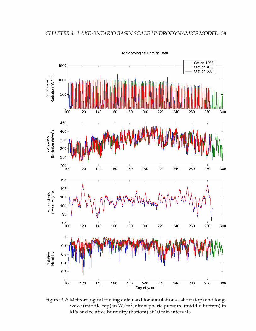
Figure 3.2: Meteorological forcing data used for simulations - short (top) and long-wave (middle-top) in W/m2, atmospheric pressure (middle-bottom) inkPa and relative humidity (bottom) at 10 min intervals.

CHAPTER 3. LAKE ONTARIO BASIN SCALE HYDRODYNAMICS MODEL 39
Figure 3.3: Rain and tributary flow (top) in m over the lake surface, Welland Canaland Niagara River inflows with north and south St. Lawrence Riveroutflows (middle) in m3/s and total major inflows and outflows (bot-tom) in m3/s.
CHAPTER 3. LAKE ONTARIO BASIN SCALE HYDRODYNAMICS MODEL 40
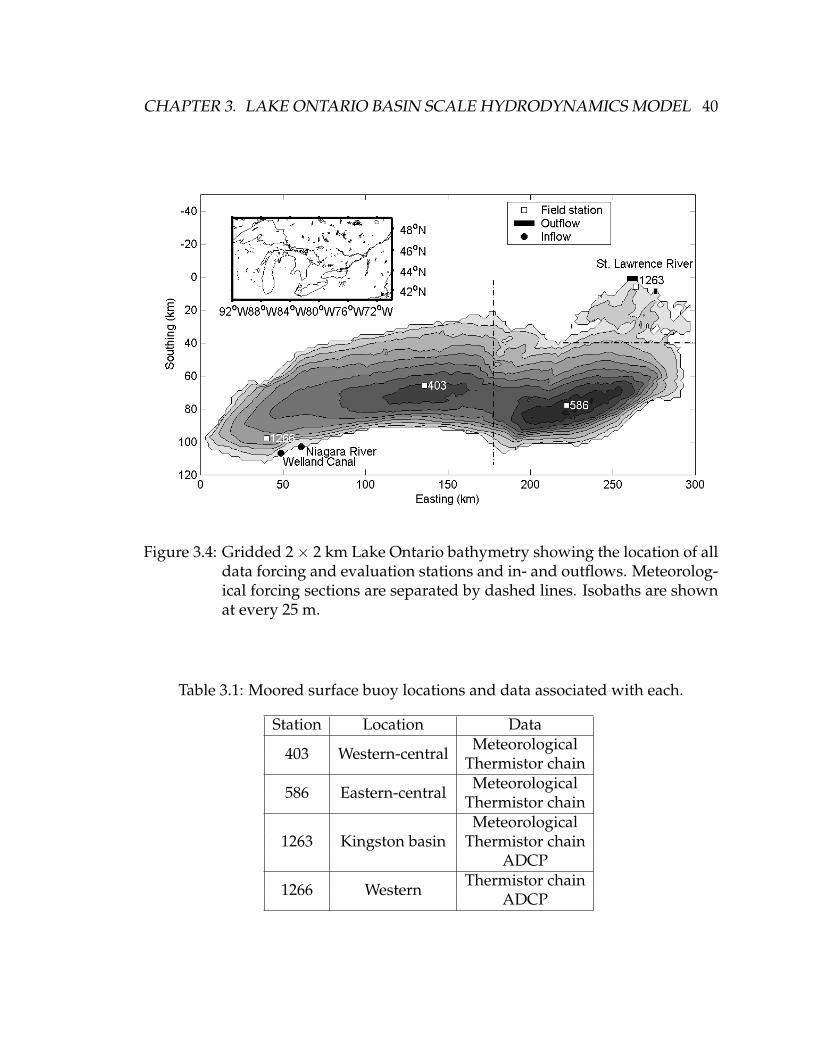
Figure 3.4: Gridded 2 × 2 km Lake Ontario bathymetry showing the location of alldata forcing and evaluation stations and in- and outflows. Meteorolog-ical forcing sections are separated by dashed lines. Isobaths are shownat every 25 m.
Table 3.1: Moored surface buoy locations and data associated with each.
Station Location Data
403 Western-central MeteorologicalThermistor chain
586 Eastern-central MeteorologicalThermistor chain
1263 Kingston basinMeteorological
Thermistor chainADCP
1266 Western Thermistor chainADCP

CHAPTER 3. LAKE ONTARIO BASIN SCALE HYDRODYNAMICS MODEL 41
3.2.3 Simulations
The summer season is of interest in this study because of the lake’s baroclinic na-
ture and the complex thermally driven circulation associated with it. There is am-
ple evidence showing that basin-scale internal waves on the thermocline provide
the driving forces for vertical and horizontal fluxes in a stratified lake beneath the
surface layer [14]. However, the purpose of this study is to model the first order
properties of Lake Ontario’s circulation, the setup and decay of stratification and
the mean currents in the offshore and nearshore reagions. With the lake’s internal
Rossby Radius of the order of 5 km, Kelvin waves cannot be resolved with a grid
size of 2 × 2 km. Internal wave motions as simulated in ELCOM are described by
Hodges et al. [14].
ELCOM simulations lasted approximately 2.5 days starting on day 101 of 2006
(April 11) well before the onset of temperature stratification which allows for a
uniform initial temperature of 3.4◦C in the lake. The initial water temperature of
the lake was calculated from the available thermistor chain data from stations 403,
586 and 12664. This start date also permits capturing the entire onset of stratifica-
tion. The simulation time-step is 5 min, as used in a similar model of Lake Erie by
Leon et al., as it was shown to give the best results at an acceptable computational
efficiency [6]. ELCOM can interpolate for a smaller time-step when its forcing data
time-step is larger [29] as it is 10 min for this model. Simulations end on day 299
(October 26, 2006) giving a large enough window into the baroclinic hydrodynam-
ics of the lake allowing for the visualization of the onset of stratification as well
as the beginning of its deterioration and the lake’s return to barotropic conditions
4Observed water temperature and current profile data was provided by C. H. Marvin, R.Yerubandi and B. Schertzer at NWRI

CHAPTER 3. LAKE ONTARIO BASIN SCALE HYDRODYNAMICS MODEL 42
(Figure 3.5).
For effective model evaluation, simulated temperature profiles, currents and
water levels were compared to observed data. ELCOM simulations were com-
pared with thermistor chain data and ADCP data from 2006 provided by the Na-
tional Water Research Institute (NWRI)5 as well as historic water level data ob-
tained from a variety of different gauges around the lake [45]. Thermistor chain
data was collected with Tidbit data loggers with 12-bit resolution and a precision
sensor with 0.2◦C accuracy over a temperature range between -20 and 30◦C [46].
ADCP data was measured at every meter throughout the water column with a
velocity resolution of 0.125 to 0.25 cm/s and an accuracy of 0.5 cm/s [47].
3.3 Results
3.3.1 Temperature Profiles
Observed temperature data recorded every 10 min from the four moorings were
were compared to modelled output at 10 min intervals. The modelled temper-
ature data was plotted using values from the same depths as the observed data
recorded from thermistor chains. Figures 3.5, 3.6, 3.7 and 3.8 show the measured
and simulated temperature profiles of the entire water column at each of the four
stations throughout the lake where thermistor chains were located. Maximum rate
of temperature change portraying the thermocline occurs between temperatures
of about 13 to 20◦C once stratification has set in for temperature profiles at stations
403, 586 and 1266. Water depth at station 1263 is too shallow for the occurrence of
5Observed water temperature current data was provided by C. H. Marvin, R. Yerubandi and B.Schertzer at NWRI
CHAPTER 3. LAKE ONTARIO BASIN SCALE HYDRODYNAMICS MODEL 43
temperature stratification, therefore the entire water column is uniformly warmed
with depth.
With the effect of scaling the shortwave radiation by 0.9 and the long-wave ra-
diation by 1.15, ELCOM satisfactorily simulates temperature at all stations in the
lake both in the nearshore regions and the offshore regions. Small differences in
modelled to observed temperature profiles should be expected because of the use
of such a coarse grid scale. As there are a total of four thermistor chains spread
out over the entire lake with which observed data was collected to evaluate simu-
lations, it can be inferred that ELCOM properly replicates the temperature stratifi-
cation in the entire lake.
Both modelled and observed temperature profiles show that the water at sta-
tion 1263 warms almost consistently throughout the depth of the water column
although the top of the water column warms faster with respect to the bottom
then is observed in the field data. Cooling is shown to be constant with depth for
the observed data in the fall at station 1263 but the bottom is cooler throughout
the simulation in the model. ELCOM’s tendency to underestimate temperature is
exemplified in the modelled profile at this station because of the shallow depth of
the water column compared to the greater depth of the three other locations. The
model portrays an infusion of cooler water around day 230 but warmer water is
observed at that time. It is difficult to compare the success of nearshore tempera-
ture profiles to that of offshore temperature profiles because of the great difference
in their depth.
The deepest temperature profile comparison is at station 586 where warming
of surface water looks to be slightly premature compared to the observed data.

CHAPTER 3. LAKE ONTARIO BASIN SCALE HYDRODYNAMICS MODEL 44
Figure 3.5: Modelled (top) and observed (bottom) temperature profiles at station1263 at 10 min intervals. Modelled temperature output was interpo-lated at 1, 3, 5, 7 and 10 m depths to match observed data.

CHAPTER 3. LAKE ONTARIO BASIN SCALE HYDRODYNAMICS MODEL 45
Figure 3.6: Modelled (top) and observed (bottom) temperature profiles at station586 at 10 min intervals. Modelled temperature output was interpolatedat 2.7, 4, 6, 8, 12, 14, 16, 18, 20, 22, 24, 26, 30, 35, 40, 50, 100 and 150 mdepths to match observed data.

CHAPTER 3. LAKE ONTARIO BASIN SCALE HYDRODYNAMICS MODEL 46
Smearing of the pycnocline is slightly exaggerated by in the modelled results as
well. The cool water observed around day 250 is properly captured by the model
but the modelled thermocline reestablishes too low and modelled water in the epil-
imnion is therefore warmer than observed. The thermocline depth at this station
looks to compare well but because of the depth of the water column in this area of
the lake, small differences in thermocline depth between modelled and observed
profiles are difficult to distinguish. Another example of ELCOM’s tendency to un-
derestimate temperatures occurs between days 175 and 200 at this station as the
modelled thermocline depth is higher in the modelled profile compared to obser-
vations.
In the modelled temperature profile at station 403, the gradual warming of the
water with depth starts immediately whereas, warming in the observed profile
starts suddenly at a depth of 30 m around day 130. The thermocline is observed
to establish itself at a depth of about 25 m around day 190 and the modelled pro-
file shows it establishing at the same time but at a depth well above 20 m. The
modelled thermocline does not look as sharp as it does in the observed profile.
The modelled temperature profile does not capture the extent of the cooling event
from day 145 to 155. However, the start date of stratification deterioration is well
captured by the model.
The modelled temperature profile at station 1266 reproduces the small warm-
ing event before the onset of stratification at day 115. The observed depth of
the thermocline is slightly greater than the modelled results. This is opposite to
the comparison at station 403. The observed vertical transport of heat in the hy-
polimnion is not efficiently captured by the model. A small cooling event just prior
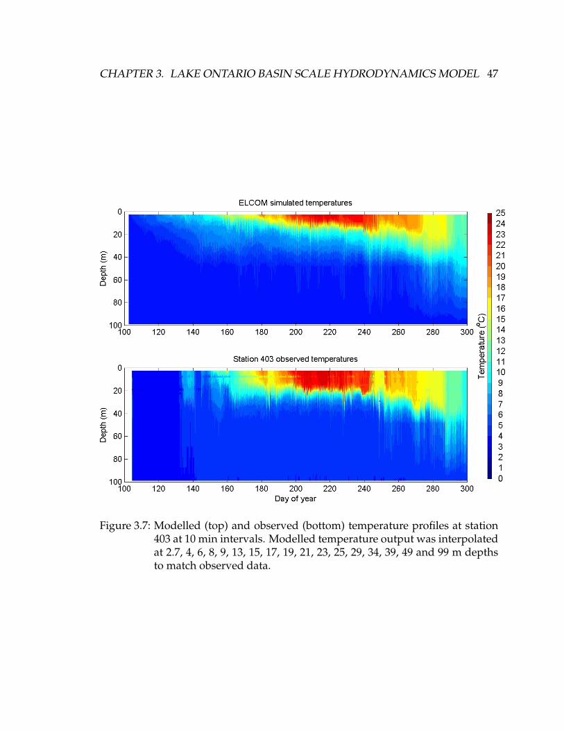
CHAPTER 3. LAKE ONTARIO BASIN SCALE HYDRODYNAMICS MODEL 47
Figure 3.7: Modelled (top) and observed (bottom) temperature profiles at station403 at 10 min intervals. Modelled temperature output was interpolatedat 2.7, 4, 6, 8, 9, 13, 15, 17, 19, 21, 23, 25, 29, 34, 39, 49 and 99 m depthsto match observed data.
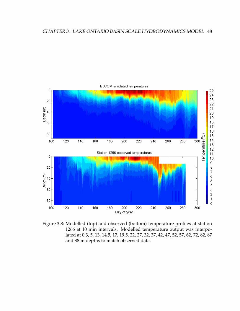
CHAPTER 3. LAKE ONTARIO BASIN SCALE HYDRODYNAMICS MODEL 48
Figure 3.8: Modelled (top) and observed (bottom) temperature profiles at station1266 at 10 min intervals. Modelled temperature output was interpo-lated at 0.3, 5, 13, 14.5, 17, 19.5, 22, 27, 32, 37, 42, 47, 52, 57, 62, 72, 82, 87and 88 m depths to match observed data.

CHAPTER 3. LAKE ONTARIO BASIN SCALE HYDRODYNAMICS MODEL 49
to day 180 is not shown in modelled results. When stratification is strongest, be-
tween days 190 and 230, there is less vertical transport of heat in the hypolimnion
in both the observed and modelled profiles. Lastly, modelled results do not capture
the extent of the depth of the event just before day 250.
3.3.2 Water Levels
A literature search for previous work reporting on ELCOM water level simula-
tions was performed with no success. Verifying ELCOM water levels as well as
temperature results with field data are of particular importance to this study. The
modelled water level and temperature profiles can be used to force an open bound-
ary for simulating the hydrodynamics of a fine-grid model of the nearshore area
in the Kingston basin and the upper St. Lawrence River. This could provide more
precise hydrodynamic results in the nearshore area.
The model was initially forced including only outflow at the St. Lawrence
River, rain and inflows from the Niagara River and the Welland Canal. Figure
3.9 shows the water level comparisons at Kingston when only major inflows, out-
flows and rain are modelled. The water levels are plotted hourly to show surface
level fluctuation as well as daily mean values giving a clearer view of the seasonal
rise and fall of the lake surface.
Figure 3.9 shows steadily declining water levels with a difference of 0.41 m at
peak water levels with respect to the observed. The modelled water level contin-
ues to diverge from observed water levels and near the end of the simulation there
is a difference of 0.55 m. Therefore, including only major inflows, outflows and
rain in ELCOM simulations does not account for all the components in the lake’s

CHAPTER 3. LAKE ONTARIO BASIN SCALE HYDRODYNAMICS MODEL 50
Figure 3.9: Modelled and observed hourly (top) and daily (bottom) water levelfluctuations at station 1263. Simulation includes major inflows, out-flows and precipitation.

CHAPTER 3. LAKE ONTARIO BASIN SCALE HYDRODYNAMICS MODEL 51
water balance. In most lakes tributary and overland flow is considered negligible.
Because of the size of Lake Ontario and its drainage basin, tributary and over-
land flow accounts for about 14% of all Lake Ontario inflow [44]. The modelled
monthly tributary data was provided in metres over the lake surface. These val-
ues were divided into daily totals and scaled to correspond to the amount of daily
precipitation associated with each day. Scaled tributary values were then added
to the precipitation values uniformly over the lake surface as shown in Figure 3.3.
Modelled results including tributary flows are shown in Figure 3.10.
Figure 3.10: Modelled and observed hourly (top) and daily (bottom) water levelfluctuations at station 1263. Simulation includes modelled tributaryflow, precipitation and major inflows and outflow.

CHAPTER 3. LAKE ONTARIO BASIN SCALE HYDRODYNAMICS MODEL 52
With the added modelled tributary data, the simulated water levels compare
well for the first 40 days of the simulation and then the simulated and observed
water levels start to diverge and the ELCOM water levels end up about 0.12 m
lower then the peak observed water levels. Modelled water levels at various loca-
tions around the lake were compared to historical data in nearby locations to verify
that the model is performing equally well all around the lake. As water level re-
sults were all satisfactory and the Kingston basin area is of interest as well as for
brevity, the results are not shown for these simulations.
3.3.3 Currents
The goals of this study are to test the ELCOM’s ability to represent offshore and
nearshore water movement. Therefore, it is necessary not only to look at how
well ELCOM simulates temperature fluctuations in the water column and water
level fluctuations but to look at how modelled currents compare with observed
data. Current observations were available for the second half of the simulation at
station 1266 and for the first half of the simulation at station 1263.
Currents at station 1266 (Figure 3.11) in the hypolimnion range between 5 and
-5 cm/s. The water above the thermocline reaches speeds much higher then in the
hypolimnion. However, events of increased east or west velocities are observed
throughout the water column but are not reproduced at depth in the ELCOM sim-
ulation. The event seen in the observed temperature profile for station 1266 around
day 250 is also portrayed in the observed east component of velocity profile with
a smaller representation in the observed north component profile. Like in the tem-
perature profile comparisons, ELCOM current profiles do not capture the extent

CHAPTER 3. LAKE ONTARIO BASIN SCALE HYDRODYNAMICS MODEL 53
Figure 3.11: Modelled north (a) and east (c) components of velocity compared tonorth (b) and east (d) components of observed velocity at station 1266at daily intervals. Observed velocity was measured at 2 m intervalsthroughout the water column.

CHAPTER 3. LAKE ONTARIO BASIN SCALE HYDRODYNAMICS MODEL 54
of this event. Increases in the north component of observed velocity previous and
after this event are weakly reproduced in ELCOM. Generally ELCOM does not re-
produce currents to the entire depth at which they are observed. ELCOM shows
an increased westward water movement in the modelled epilimnion which is not
evident in the observed data. Observed temperature data for this period is unavail-
able making interpretation of this portion of the current profiles very difficult.
The observed north component of velocity at station 1263 (Figure 3.12) varies
only between 5 and -5 cm/s before day 160 which coincides with the date that
water at this location starts to significantly warm. Increased water velocities and
mixing in this shallow area facilitates the warming of the entire water column. EL-
COM simulated north component of velocity in the top 5 m of the water column
is too high in magnitude compared to observed data previous to day 160. After
day 160, ELCOM does a good job of reproducing the currents in the top 5 m of the
water column. However, the mid portion of the simulated water column portrays
a north velocity slightly higher than what is observed. Very little water movement
is observed in the east-west direction. ELCOM greatly over estimates this for the
entire simulated time period shown. ELCOM also portrays much more west mov-
ing water in the bottom portion of the water column than is observed between day
160 and 210. Once the water in the entire depth of the water column has warmed
(after day 160), ELCOM shows a consistent north-westerly water current direction
for the bulk of the water column below a 5 m depth. However, it is however ob-
served that the flow direction switched back and forth fairly consistently between
north-west and south-east directions.

CHAPTER 3. LAKE ONTARIO BASIN SCALE HYDRODYNAMICS MODEL 55
Figure 3.12: Modelled north (a) and east (c) components of velocity compared tonorth (b) and east (d) components of observed velocity at station 1263at daily intervals. Observed velocity was measured at 1 m intervalsthroughout the water column.

CHAPTER 3. LAKE ONTARIO BASIN SCALE HYDRODYNAMICS MODEL 56
Although current profiles give a good idea of how well the model is perform-
ing, only simulated temperature profiles and water levels are needed to force an
open boundary in ELCOM. Grid size plays a significant role in how accurate the re-
sults are especially in the nearshore region as bathymetry plays a larger role in de-
termining water movement because of the shallower water depth. In the offshore
region, ELCOM currents compare well to measured data (Figure 3.11). However,
in the nearshore region, results are less accurate (Figure 3.12). The difference be-
tween modelled and observed velocity was plotted and is shown in Appendix ??.
3.4 Discussion
3.4.1 Temperature Evaluation
Temperature profiles are an excellent means of visualizing basin-scale waves [4,
10, 12, 20, 27] and have been a main component of numerical model evaluations
as seen in literature [6, 14, 19, 30]. For confidence that the model is adequately re-
producing the hydrodynamics in the entire lake, it is important that there be good
agreement between observed and simulated temperature profiles throughout the
lake.
Long and shortwave radiation as well as air temperature are the components
of meteorological forcing that most prominently effect the lake’s simulated tem-
peratures. It was found that using the method of scaling seen in Laval et al. gave
the best agreement between ELCOM simulated results and observed data. How-
ever, even with these scaling factors, ELCOM is shown to underestimate modelled
temperature at station 1263. Scaling factors of 1.15 and 0.9 for long- and shortwave

CHAPTER 3. LAKE ONTARIO BASIN SCALE HYDRODYNAMICS MODEL 57
radiation were used for Lake Kinneret simulations [28]. Lake Kinneret is a much
smaller lake requiring less energy to heat. Further simulations would be required
to obtain scaling coefficients for long and shortwave radiation unique to Lake On-
tario.
The simulation length is of importance because results portray the setup and
deterioration of stratification. The variation in depths of the station locations, from
the shallow waters of station 1263 in the Kingston basin to the deepest portion of
the lake at station 586, allows for the visualization of the temperature variations in
areas of different depths. However, because of the large variance in depth of the
nearshore and offshore temperature profiles, it is difficult to determine if ELCOM
better reproduces temperature stratification in the offshore or nearshore profiles.
The observed temperature profile at station 1266 (Figure 3.8) shows evidence
of a storm event that was not captured to the same depth in the model. This could
be attributed to the great distance between station 1266 and the closest moored
weather station (Figure 3.4) and therefore the intensity of this storm was not accu-
rately captured by these results. Therefore spatially varied meteorological forcing
is essential when modelling large lakes and this model of Lake Ontario may benefit
from more varied meteorological forcing files. Evidence of this event is also appar-
ent in the temperature profiles at stations 586 and 403 (Figure 3.6 and 3.7) where
during this time period the simulated temperature is warmer then the observed
data. This is opposite to the rest of the simulation period and could be associated
with the event recorded on the observed profile at station 1266. Therefore, it is pos-
sible that other localized storm events not captured by the meteorological forcing
files could be the cause of variance between observed and simulated temperature

CHAPTER 3. LAKE ONTARIO BASIN SCALE HYDRODYNAMICS MODEL 58
profiles.
3.4.2 Water Level Evaluation
It has been previously found that the Niagara and the St. Lawrence Rivers have
little impact on the overall modelled circulation of the lake and that any impact is
mostly confined to a region in the order of 10 km from each respective river [5].
However, all inflows and outflows to and from the lake are important for mod-
elling water level fluctuations. Evaluation of modelled water level fluctuations is
a method of assuring that the model accurately represents all the hydrodynamic
processes in the lake. (See Appendix B for more information on the importance of
water level evaluation.) Previous to this, the literature has not covered ELCOM’s
performance with predicting water levels. Evaluating the water levels is of partic-
ular importance for this study as the water levels produced by this model can be
used to force an open boundary to a finer grid model.
Modelling the water balance of Lake Ontario has many flaws. Its large drainage
basin, many minor tributaries and overland flow are variables which are difficult
to accurately monitor. Both rain and tributary flow data is accounted for in me-
tres over the surface of the lake. Therefore the surface area of the modelled lake
directly influences the volume of water input into the the model through these
variables. Because of the coarse 2 × 2 km grid, the modelled surface area of the
lake may not match the surface area that these variables are based on which could
account for the discrepancy between the modelled and observed water levels. It
must also be noted that groundwater is not accounted for in these simulations,
however the deficit between modelled and observed water levels is not constant

CHAPTER 3. LAKE ONTARIO BASIN SCALE HYDRODYNAMICS MODEL 59
and therefore neglecting groundwater flow cannot be directly responsible for this
deficit although it may play a part.
In Figure 3.10, the modelled water levels match the observed data until about
40 days into the simulation where the modelled water levels start to diverge away
from the observed. This could be due to the significant amount of precipitation
that the lake receives starting around that time but is not accurately represented
in the model because the volume of water from precipitation and tributary data is
dependant on surface area and it is not known if the surface area of the modelled
lake and area of which the data is based from are the same. This could account for
the difference in modelled and observed water levels.
The ELCOM simulated water levels compare relatively well to the observed
data considering the size of the lake and its drainage basin as well as the of lack
accurate forcing data for tributaries, overland flow and rain. In an effort to deter-
mine how much water is missing in the ELCOM simulated system, the tributary
data was scaled. By trial and error, it was found that scaling the modelled tribu-
tary data by a factor of 1.2 gives optimal results as shown in Figure 3.13. Increasing
the tributary data by a factor of 1.2 reduces the difference between observed and
modelled peak water levels to 0.01 m.
3.4.3 Current Evaluation
North and east components of velocity comparisons are another common way of
evaluating the effectiveness of a model at representing the hydrodynamics in a
lake. Current meter data was available for two locations in the lake, at station 1266
offshore in the western side of the lake and station 1263 nearshore in the Kingston

CHAPTER 3. LAKE ONTARIO BASIN SCALE HYDRODYNAMICS MODEL 60
Figure 3.13: Modelled and observed hourly (top) and daily (bottom) water levelfluctuations at station 1263. Simulation includes scaled tributary flow,precipitation, major inflows and outflow.
CHAPTER 3. LAKE ONTARIO BASIN SCALE HYDRODYNAMICS MODEL 61
basin. The simulated currents at station 1266 compared better with observed data
than current comparisons at station 1263. For the most part, the observed and sim-
ulated currents are not very strong, particularly below a 5-10 m depth, therefore
small differences between observed data and simulated results are not of great
significance. However, ELCOM does not capture the entire depth of the currents
represented in the observed data. This may be attributed to numerical diffusion
problems also seen in Laval et al. and Hodges et al. [11, 14, 19, 30] or, as mentioned
above, the inability of the weather station at station 403 at capturing the extent of
the storm event around day 150 in the vicinity of station 1266.
The the bathymetry of the nearshore region of station 1263 may have influenced
poorer results compared to current profiles at station 1266 where the depth of the
water column is almost 10 times deeper. In the nearshore region of station 1263,
actual bathymetry is much more complicated than can be captured on a 2 × 2 km
grid scale. Because of the shallow depth in this region, this could have a significant
effect on simulated currents more so than in the deep water region of station 1266.
Simulated currents for the bottom portion of the water column at station 1263 after
day 160 are shown to be much smoother than observed. The extent of influence
that bathymetry has on water movement in ELCOM is unknown but could still
be a factor in contributing for the discrepancies between modelled and observed
current profiles at this station. The direction of outflow in ELCOM could also play
a role in contributing to the differences between modelled and observed current
profiles at station 1263 because of the outflow’s proximity to this station. The sim-
ulated outflow near this location is a straight east-west opening but in reality the
flow curls north-east around Wolfe Island. The coarseness of the grid prevents an

CHAPTER 3. LAKE ONTARIO BASIN SCALE HYDRODYNAMICS MODEL 62
accurate representation of this outflow and the bathymetry around this nearshore
region. This could have a negative effect on simulated currents and be another
component leading to discrepancies between modelled and simulated currents.
Because of the greater depth and simple bathymetry at station 1266, the current
comparisons are much more satisfactory (Figure 3.14).
Figure 3.14: Observed bathymetry (a) compared to ELCOM 2 × 2 km grid (b) atnearshore station 1263 and observed bathymetry (c) compared to EL-COM 2 × 2 km grid (b) at offshore station 1266
Overall, current comparisons are much more variable than temperature profile

CHAPTER 3. LAKE ONTARIO BASIN SCALE HYDRODYNAMICS MODEL 63
comparisons. However, it is important to note that in order to provide forcing for
an open boundary simulation in ELCOM only temperature profiles and water level
fluctuations are required, current profiles are not needed. Also, simulating such an
open boundary should be done in the mid-lake area away from any complicated
bathymetry near the shoreline or outflows in order to be sure that the modelled
data forcing the open boundary is accurate.
The ELCOM model was compared to observed 2006 summer season field data
and for a holistic view of the circulation patterns it was compared with Beletsky et
al.’s plot of summer circulation [8]. Beletsky et al.’s plot, shown in Figure 3.15, was
constructed from an average of currents measured at depths of 15, 19, 30, 50 and
75 m therefore an output of averaged currents at these same depths are shown in
Figure 3.16 for the 2006 summer simulation. Certain features of this figure com-
pare well with Beletsky et al.’s plot of summer circulation. The cyclonic gyre which
Beletsky et al. observed to be very stable is very well reproduced with the ELCOM
simulation. The coastal current on the south shore of the lake also compares well.
However, the ELCOM simulation portrays several small anticyclonic gyres as op-
posed to just one in the northwestern part of the lake as is shown by the Beletsky
et al. plot. As well, a significant amount of water from the Niagara River seems
to be circulating west which also is not shown on the Beletsky et al. plot. The
differences between these two plots can be attributed to seasonal variations as the
circulation in the western part of Lake Ontario has been previously shown to be
different in different years [8]. Confidence is ensured that ELCOM is properly
representing the currents in Lake Ontario because the stable features of summer
circulation compare well to the ones mapped out by Beletsky et al. [8]. Averaged

CHAPTER 3. LAKE ONTARIO BASIN SCALE HYDRODYNAMICS MODEL 64
lake-wide currents at various depths were compared with other circulation maps
of Lake Ontario from literature in Appendix C. It should be noted that interannual
variability is not the focus of this study and has not been systematically studied in
the past. However, past studies have indicated variations in summer circulation
from year to year [8].
Figure 3.15: Beletsky et al.’s plot of summer circulation [8].
The focus of this study was to reproduce general lake circulation patterns in
the nearshore and offshore regions and ELCOM’s ability to reproduce high fre-
quency waves was not the goal of this study. Therefore whether or not, ELCOM
reproduces coastal jets, Poincare and Kelvin waves is not examined as a horizon-
tal grid scale of 2 × 2 km is to large to capture these basin-scale waves. A finer
grid scale may be more appropriate in reproducing these higher frequency waves.
Additional simulated temperature and current profile output at more locations
throughout the lake and at lower time frequencies would be necessary to identify
internal waves and their frequencies.

CHAPTER 3. LAKE ONTARIO BASIN SCALE HYDRODYNAMICS MODEL 65
Figure 3.16: Lake-wide ELCOM mean circulation for May to October 2006 inte-grated at 15, 19, 30, 50 and 75 m depths.
3.5 Conclusion
The review and consideration of previous work relating to the circulation and
modelling attempts also provided valuable information towards the successful
completion of this project. To ensure that ELCOM properly simulates the hydro-
dynamics in Lake Ontario, modelled temperature profiles, water level fluctuations
and current profiles were compared with available observational data. Agreement
between modelled and observed temperature profiles was the most successful of
the three as near- and offshore profiles compared equally well. The date at which
stratification occurs, the depth of the thermocline as well as general temperatures
were compared. Results were generally satisfactory for a coarse grid model ex-
cept that even after scaling the long- and shortwave radiation, ELCOM’s simulated

CHAPTER 3. LAKE ONTARIO BASIN SCALE HYDRODYNAMICS MODEL 66
temperatures were still slightly lower than observed.
It was of particular importance to evaluate ELCOM’s performance with wa-
ter levels as it has not previously been studied. Water level simulation results were
also compared because they can be used to force an open boundary for a nearshore
model of the Kingston basin and the upper portion of the St. Lawrence River. Wa-
ter level simulation proved to be problematic because of the lake’s size. Although
major inflow and outflow data is easily acquired, rain as well as tributary and
overland flows are provided as average values dependant on the lake surface area.
More precise data is needed for better results. Tributary forcing data was increased
by 20% to account for missing water volume.
Simulated to observed current profile agreement proved to be more variable
than temperature profiles. Simulated currents in the offshore region at station
1266 had overall better agreement with observed data than at station 1263 in the
nearshore. This can be attributed to the difference in depth between observation
sites. In the shallow area where station 1263 is situated, the movement of water
could be affected by bottom topography. Station 1263 is also near the outflow to
the St. Lawrence River. The varied bathymetry and flow out of the lake is not prop-
erly captured by the coarse 2 × 2 km grid negatively effecting the current profiles
at this location.
It was found that ELCOM does an equally good job at reproducing offshore
and nearshore temperature profiles, however simulated to observed current pro-
file comparisons agreed better in the offshore region then in the nearshore region
on a coarse grid scale. The comparisons of temperature profiles, water level fluc-
tuations and current profiles portrayed above give the confidence that, under the
CHAPTER 3. LAKE ONTARIO BASIN SCALE HYDRODYNAMICS MODEL 67
present forcing data, ELCOM does an overall good job at representing the general
circulation patterns in the offshore regions of Lake Ontario on a coarse grid scale.
It was found that the nearshore areas are not sufficiently resolved with a 2 × 2 km
grid scale to properly simulate currents and that water level simulation requires
more precise forcing data to obtain accurate results without scaling factors.
Considering all methods of evaluation, ELCOM does a good job at taking un-
averaged, spatially varied meteorological forcing data as well as inflow and out-
flow data to accurately reproduce thermal stratification and general circulation
patterns in Lake Ontario. It is also demonstrated that it is essential to model all
inflows and outflows to properly simulate lake water level fluctuations. The occur-
rence of high frequency waves was not evaluated in this study. Temperature pro-
files and scaled water level results from this study are used in Chapter 4 to force an
open boundary to better resolve nearshore hydrodynamics in the Kingston basin
and the upper portion of the St. Lawrence River and provide scientific information
to advance the CRCA study and the delineation of IPZs.

Chapter 4
Nearshore Hydrodynamic Model
4.1 Introduction
The Great Lakes have many functions including providing source drinking water
and a sink for pollutants and runoff [1]. Serious water quality problems have been
identified within the Great Lakes basin as a result of increased urbanization and
industrial activity which is generally the cause of environmental degradation of
many nearshore areas due to municipal and industrial discharge [32]. Although
substantial advances have been made in the regulation of outfall location and per-
missible effluent quality, the ever increasing total volumes of wastewater heightens
the need to understand coastal physical processes in greater detail [2].
Circulation in the Great Lakes has been of interest since the late 19th century
for a variety of applications. Most recently, due to the Clean Water Act passed
in October 2006 by the Ontario government, the responsibility of drinking water
protection has been placed in the hands of each municipality. The Ontario Clean
68

CHAPTER 4. NEARSHORE HYDRODYNAMIC MODEL 69
Water Act is intended to ensure communities take the appropriate steps in protect-
ing their drinking water supply through developing locally driven, science-based
protection plans [33]. Hydrodynamic modelling provides the basis for simulating
transport in response to meteorological forcing functions [6].
Computational requirements for lake-wide modelling is of concern. To avoid
unmanageable computation times grid scale resolutions are coarse as in the case
of the study by Hurdowar-Castro et al. who modelled the nearshore along the
Toronto waterfront on a 500 m grid scale in order to evaluate the optimum po-
sition for a new drinking water intake. The results of this model alone were not
conclusive due to the coarseness of the grid size. A smaller model with a 100 m
grid scale was nested and validated with separate drogue experiments to improve
study results which were then used to evaluate proposed locations of potential
drinking water intakes [1].
Shen et al. nested a 500 m square grid of the Lake Ontario Toronto waterfront
in a 2 km coarse grid model. The three-dimensional hydrodynamic/water quality
model was successfully validated and results were used to simulate current and
pollutant transport for a period of 5 days for both stratified and isothermal condi-
tions [32].
A two-dimensional finite element model (FEM) of the entire lake with grid sizes
varying between 80 m and 5 km have also been seen. Hayashida et al. modelled
Lake Ontario using idealized meteorological forcing data with constant Niagara
flows of 5000 m3/s and 7000 m3/s and concluded that models which do not in-
clude the whole lake may not be able to simulate the trajectory and dispersion of
Niagara River water properly under all conditions [37].
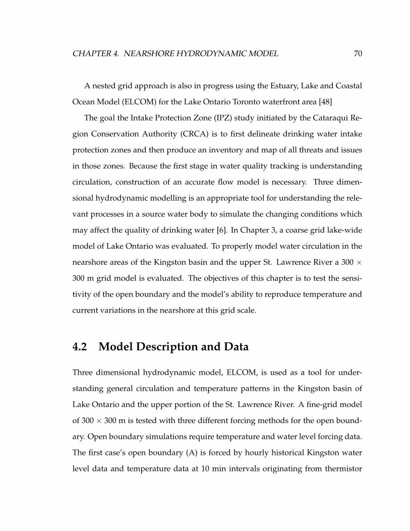
CHAPTER 4. NEARSHORE HYDRODYNAMIC MODEL 70
A nested grid approach is also in progress using the Estuary, Lake and Coastal
Ocean Model (ELCOM) for the Lake Ontario Toronto waterfront area [48]
The goal the Intake Protection Zone (IPZ) study initiated by the Cataraqui Re-
gion Conservation Authority (CRCA) is to first delineate drinking water intake
protection zones and then produce an inventory and map of all threats and issues
in those zones. Because the first stage in water quality tracking is understanding
circulation, construction of an accurate flow model is necessary. Three dimen-
sional hydrodynamic modelling is an appropriate tool for understanding the rele-
vant processes in a source water body to simulate the changing conditions which
may affect the quality of drinking water [6]. In Chapter 3, a coarse grid lake-wide
model of Lake Ontario was evaluated. To properly model water circulation in the
nearshore areas of the Kingston basin and the upper St. Lawrence River a 300 ×
300 m grid model is evaluated. The objectives of this chapter is to test the sensi-
tivity of the open boundary and the model’s ability to reproduce temperature and
current variations in the nearshore at this grid scale.
4.2 Model Description and Data
Three dimensional hydrodynamic model, ELCOM, is used as a tool for under-
standing general circulation and temperature patterns in the Kingston basin of
Lake Ontario and the upper portion of the St. Lawrence River. A fine-grid model
of 300 × 300 m is tested with three different forcing methods for the open bound-
ary. Open boundary simulations require temperature and water level forcing data.
The first case’s open boundary (A) is forced by hourly historical Kingston water
level data and temperature data at 10 min intervals originating from thermistor

CHAPTER 4. NEARSHORE HYDRODYNAMIC MODEL 71
chain data from temporary mooring 12631 in the Kingston basin in close proximity
to the location of the open boundary. The second simulation (B) was forced using
hourly historical Kingston water level data and hourly surface temperature from
Environment Canada permanent mooring C45135 located at 43.79◦N and 76.87◦W
outside of the simulated area and the Kingston basin. The third and final open
boundary simulation (C) is forced using hourly temperature and water level data
output from the coarse grid model presented in Chapter 3. The run-time of simu-
lations A and B was approximately 5 days whereas simulation C required over a
week because of the large number of files required to force the horizontally varied
open boundary condition.
ELCOM is driven by meteorological files comprised of wind speed (m/s), wind
direction (degrees clockwise from north), air temperature (◦C), relative humidity,
measured shortwave radiation (W/m2), incoming long-wave radiation (W/m2)
and atmospheric pressure (Pa) obtained from moored surface buoy 1263 (Figure
4.3) equipped with a weather station and provided by the National Water Research
Institute (NWRI). Rainfall data2 (m/day) is also included in the meteorological
forcing files. The daily rainfall values were computed using a Thiessen polygon
method which weights the observed data at every station according to its repre-
sentative area [39]. All meteorological data, including rain were input into ELCOM
at 10 min intervals (Figures 4.1 and 4.2). Realistic wind forcing has been shown to
have a significant effect on resulting circulation patterns [16]. As only the Kingston
basin and the upper portion of the St, Lawrence River are being modelled, spa-
tially varied wind forcing was not determined to be necessary to force this model.1Observed water temperature data for station 1263 was provided by C. H. Marvin, R. Yerubandi
and B. Schertzer at NWRI2Rainfall data was provided by Tim Hunter at NOAA
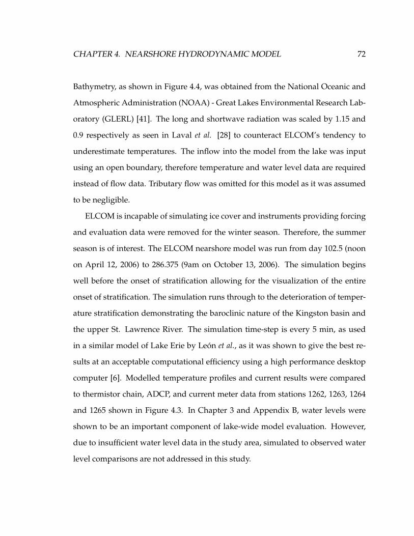
CHAPTER 4. NEARSHORE HYDRODYNAMIC MODEL 72
Bathymetry, as shown in Figure 4.4, was obtained from the National Oceanic and
Atmospheric Administration (NOAA) - Great Lakes Environmental Research Lab-
oratory (GLERL) [41]. The long and shortwave radiation was scaled by 1.15 and
0.9 respectively as seen in Laval et al. [28] to counteract ELCOM’s tendency to
underestimate temperatures. The inflow into the model from the lake was input
using an open boundary, therefore temperature and water level data are required
instead of flow data. Tributary flow was omitted for this model as it was assumed
to be negligible.
ELCOM is incapable of simulating ice cover and instruments providing forcing
and evaluation data were removed for the winter season. Therefore, the summer
season is of interest. The ELCOM nearshore model was run from day 102.5 (noon
on April 12, 2006) to 286.375 (9am on October 13, 2006). The simulation begins
well before the onset of stratification allowing for the visualization of the entire
onset of stratification. The simulation runs through to the deterioration of temper-
ature stratification demonstrating the baroclinic nature of the Kingston basin and
the upper St. Lawrence River. The simulation time-step is every 5 min, as used
in a similar model of Lake Erie by Leon et al., as it was shown to give the best re-
sults at an acceptable computational efficiency using a high performance desktop
computer [6]. Modelled temperature profiles and current results were compared
to thermistor chain, ADCP, and current meter data from stations 1262, 1263, 1264
and 1265 shown in Figure 4.3. In Chapter 3 and Appendix B, water levels were
shown to be an important component of lake-wide model evaluation. However,
due to insufficient water level data in the study area, simulated to observed water
level comparisons are not addressed in this study.
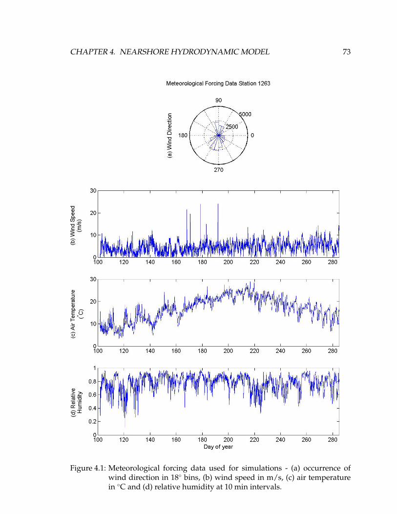
CHAPTER 4. NEARSHORE HYDRODYNAMIC MODEL 73
Figure 4.1: Meteorological forcing data used for simulations - (a) occurrence ofwind direction in 18◦ bins, (b) wind speed in m/s, (c) air temperaturein ◦C and (d) relative humidity at 10 min intervals.
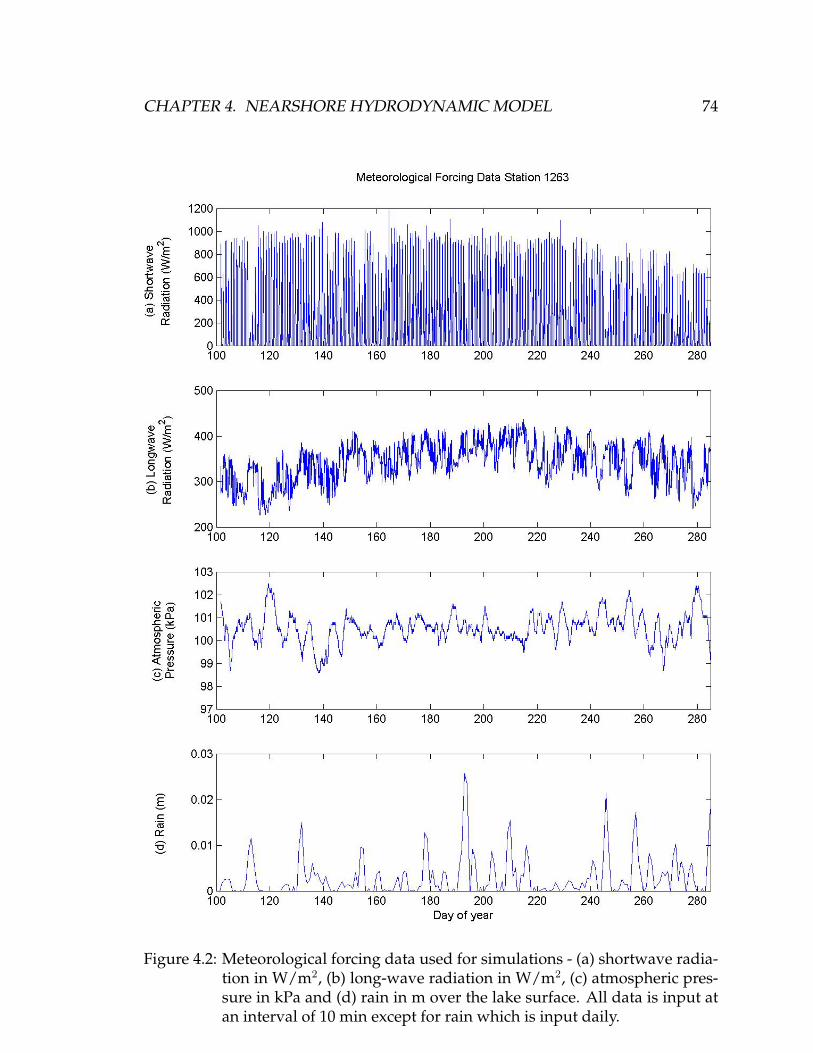
CHAPTER 4. NEARSHORE HYDRODYNAMIC MODEL 74
Figure 4.2: Meteorological forcing data used for simulations - (a) shortwave radia-tion in W/m2, (b) long-wave radiation in W/m2, (c) atmospheric pres-sure in kPa and (d) rain in m over the lake surface. All data is input atan interval of 10 min except for rain which is input daily.
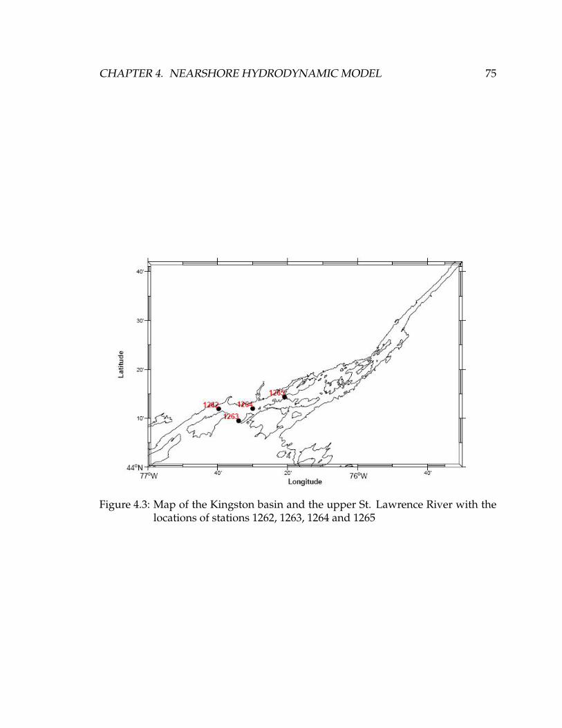
CHAPTER 4. NEARSHORE HYDRODYNAMIC MODEL 75
Figure 4.3: Map of the Kingston basin and the upper St. Lawrence River with thelocations of stations 1262, 1263, 1264 and 1265

CHAPTER 4. NEARSHORE HYDRODYNAMIC MODEL 76
Figure 4.4: Gridded 300 × 300 m Kingston basin and upper St. Lawrencebathymetry
To force an open boundary in ELCOM, both water level and water temperature
data is needed. The model outflow is simulated with water level and water tem-
perature data measured at Cornwall and obtained from Environment Canada’s
Great Lakes St. Lawrence Regulation Office3. The inflow through the North Chan-
nel is simulated with a temperature profile obtained from station 1263 and Kingston
historical water level data [45]. The water level and temperature forcing files for
the open boundary connecting the Kingston basin to the main body of Lake On-
tario were forced using three different combinations of water level and tempera-
ture data sets described above in order to determine which scenario provides the
best modelled results and how sensitive the main inflowing open boundary is to
3Inflow and outflow data was obtained Len Falkiner at Environment Canada’s Great Lakes St.Lawrence Regulation Office

CHAPTER 4. NEARSHORE HYDRODYNAMIC MODEL 77
spatially varied forcing data.
4.3 Results
4.3.1 Temperature Profiles
ELCOM results for all simulations were compared to observed temperature pro-
files recorded at 10 min intervals at stations 1262, 1263, 1264 and 1265 in Figures
4.5, 4.6, 4.7 and 4.8. Thermistor chain data at all observation stations were col-
lected with Tidbit data loggers with 12-bit resolution and 0.2◦C accuracy over a
temperature range between -20 and 30◦C [46].
At all stations, initially, simulation A temperature profiles are shown to warm
the fastest. However, simulation C shows a warming event at station 1262 and 1263
which does not compare with observed data. Simulations B and C show equally
warmer temperature profiles than simulation A at all stations locations. Results
for simulation C at stations 1264 and 1265 along with results from simulation B at
station 1265 portray warmer temperature values than is observed. All observed
profiles are shown to have fairly uniform temperatures with depth starting be-
tween days 190 to 220. Simulations B and C compare well to observed temperature
profiles at all stations. Cooling is slower in ELCOM simulations than in observed
profiles at all stations. Observed temperature profile at station 1265 shows the for-
mation of a thermocline at the bottom of the water column between days 180 and
200 which none of the ELCOM simulations at this station successfully reproduce.
Therefore the thermocline is more diffuse in ELCOM simulations, probably due to
numerical diffusion and the coarseness of the grid scale. It should also be noted
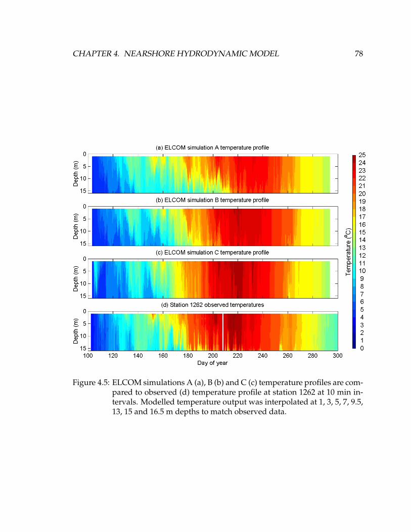
CHAPTER 4. NEARSHORE HYDRODYNAMIC MODEL 78
Figure 4.5: ELCOM simulations A (a), B (b) and C (c) temperature profiles are com-pared to observed (d) temperature profile at station 1262 at 10 min in-tervals. Modelled temperature output was interpolated at 1, 3, 5, 7, 9.5,13, 15 and 16.5 m depths to match observed data.
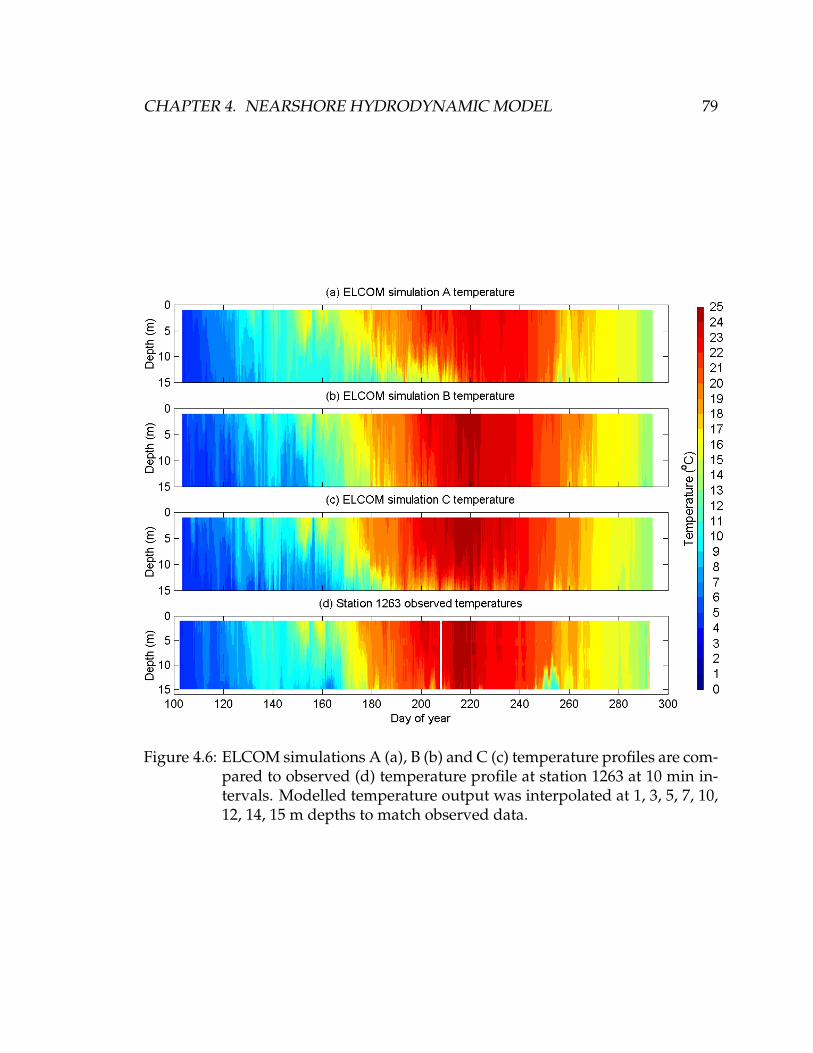
CHAPTER 4. NEARSHORE HYDRODYNAMIC MODEL 79
Figure 4.6: ELCOM simulations A (a), B (b) and C (c) temperature profiles are com-pared to observed (d) temperature profile at station 1263 at 10 min in-tervals. Modelled temperature output was interpolated at 1, 3, 5, 7, 10,12, 14, 15 m depths to match observed data.
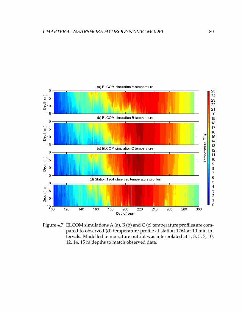
CHAPTER 4. NEARSHORE HYDRODYNAMIC MODEL 80
Figure 4.7: ELCOM simulations A (a), B (b) and C (c) temperature profiles are com-pared to observed (d) temperature profile at station 1264 at 10 min in-tervals. Modelled temperature output was interpolated at 1, 3, 5, 7, 10,12, 14, 15 m depths to match observed data.

CHAPTER 4. NEARSHORE HYDRODYNAMIC MODEL 81
Figure 4.8: ELCOM simulations A (a), B (b) and C (c) temperature profiles are com-pared to observed (d) temperature profile at station 1265 at 10 min in-tervals. Modelled temperature output was interpolated at 1 3 5 7 9.5 1315 16.5 m depths to match observed data.

CHAPTER 4. NEARSHORE HYDRODYNAMIC MODEL 82
Table 4.1: Depth averaged RMS analysis results for temperature profiles
Station Simulation A Simulation B Simulation C1262 2.35 1.87 1.811263 2.01 1.59 1.681264 1.99 1.51 1.321265 1.76 1.59 1.68
that temperature fluctuations are similar in all three simulations at station 1265.
For further comparison, a root mean squared (RMS) analysis was performed
comparing the results from all three simulations to observed data. Figures 4.9,
4.10, 4.11 and 4.12 demonstrate the results of this analysis with depth. RMS graph-
ical analysis shows that all simulated temperature profiles compare better with
observed data for the top half of the water column and that simulations B and C
show similar results which compare better to the observed data than the results for
simulation A. Table 4.1 compares the overall RMS results at each station for each
simulation.
The lower the RMS value the better simulated and observed temperature pro-
files agree. Temperature profile RMS results for each station vary slightly for each
simulation. However, no one station has consistently better or worse RMS values
which provides confidence that the model is performing equally well in terms of
temperature over the entire simulated area. Both simulation B and C had the low-
est RMS values at two stations, therefore simulations B and C performed equally
well in terms of comparing temperature profiles.

CHAPTER 4. NEARSHORE HYDRODYNAMIC MODEL 83
Figure 4.9: RMS analysis results for comparison of simulated temperature profilesand observed data for simulations A, B and C at station 1262.

CHAPTER 4. NEARSHORE HYDRODYNAMIC MODEL 84
Figure 4.10: RMS analysis results for comparison of simulated temperature profilesand observed data for simulations A, B and C at station 1263.

CHAPTER 4. NEARSHORE HYDRODYNAMIC MODEL 85
Figure 4.11: RMS analysis results for comparison of simulated temperature profilesand observed data for simulations A, B and C at station 1264.
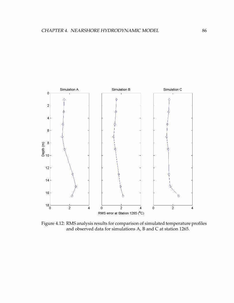
CHAPTER 4. NEARSHORE HYDRODYNAMIC MODEL 86
Figure 4.12: RMS analysis results for comparison of simulated temperature profilesand observed data for simulations A, B and C at station 1265.
CHAPTER 4. NEARSHORE HYDRODYNAMIC MODEL 87
4.3.2 Currents
Evaluating ELCOM’s performance with reproducing currents in the nearshore was
also of interest. Modelled current data was compared to observed data provided
by NWRI at stations 1262 and 1263. Station 1262 was equipped with a Nobska
MAVS-3SL current meter at a depth of 11 m with an speed and direction accuracy
of 0.3 cm/s and 1 degree respectively, as well as a resolutions of 0.03 cm/s and +2
degrees. Station 1263 was equipped with an ADCP measuring currents at every
meter throughout the water column with a velocity resolution of 0.125 to 0.25 cm/s
and an accuracy of 0.5 cm/s [47]. Unfortunately current data was not available for
the full lengths of the simulation time period. However, all data was available for
sufficient periods of time in order to compare modelled and observed data and
evaluate ELCOM’s ability to reproduce mean circulation patterns in the nearshore
area. Figure 4.13 portrays modelled to observed current meter data comparisons
at stations 1262 and Figures 4.15 and 4.14 portray modelled to observed ADCP
profiles at station 1263 for simulations A, B and C.
Modelled currents from simulations A and B are similar. At station 1262, mod-
elled currents show greater speeds and more directional variation than is observed.
Simulation C currents show larger south east velocities than observed velocities.
Although all simulated currents vary more than observed in speed and direction,
simulations A and B compare better than simulation C.
Observed currents at station 1263 were available for day 102 to 210. Modelled
currents for simulations A and B are again shown to be similar at this station. The
observed east component of velocity is weak, very seldom rising above a speed of 5
cm/s and only in the top few metres of the water column. However, the modelled

CHAPTER 4. NEARSHORE HYDRODYNAMIC MODEL 88
Figure 4.13: Simulation A, B and C north (top) and east (bottom) components ofvelocity compared to observed data at an 11 m depth at station 1262.

CHAPTER 4. NEARSHORE HYDRODYNAMIC MODEL 89
Figure 4.14: ELCOM east component of daily velocity comparison with observeddata (d) for simulations A (a), B (b) and C (c) at station 1263.

CHAPTER 4. NEARSHORE HYDRODYNAMIC MODEL 90
Figure 4.15: ELCOM north component of daily velocity comparison with observeddata (d) for simulations A (a), B (b) and C (c) at station 1263.
CHAPTER 4. NEARSHORE HYDRODYNAMIC MODEL 91
east component of velocity for all simulations reaches speeds much higher than
observed and direction is much more variable. The north component of observed
velocity is shown to reach higher speeds than the observed east component and
at a greater depth. The north component of observed data shows varied current
direction with depth. These episodes portray the top half of the water column
flowing north and the bottom half flowing south. These depth-varied currents
are seen in ELCOM simulations A and B but do not compare well. Simulation C
portrays the opposite with very strong south currents in the top three quarters of
the water column and a weak north current direction in the bottom. The difference
between modelled and observed velocity was plotted and is shown in Appendix
E.
An RMS analysis was performed comparing modelled to observed current re-
sults for station 1263 (Figure 4.16). Simulations A and B show similar results but
simulation C’s analysis shows values about twice as large as those for simulations
A and B. Therefore simulations A and B compare better to observed currents than
simulation C. Modelled currents in the bottom half of the water column agree bet-
ter with observed data for both north and east components. For the top half of
the water column, the east component of simulated velocity agrees better with ob-
served values than the north component. Mean RMS values were computed for
the entire depth of the water column at station 1263 and at a depth of 11 m for
station 1262 (Table 4.2). The simulated north component of velocity appears to
compare better to observed values than the east component for all simulations at
both stations 1262 and 1263.

CHAPTER 4. NEARSHORE HYDRODYNAMIC MODEL 92
Figure 4.16: RMS analysis results for comparison of simulated currents profilesand observed data for simulations A, B and C at station 1263.
Table 4.2: RMS analysis results for current profiles
Station Simulation A Simulation B Simulation CNorth East North East North East
1262 5.92 6.64 6.56 5.26 15.76 10.281263 3.69 2.79 3.69 2.79 11.78 6.81

CHAPTER 4. NEARSHORE HYDRODYNAMIC MODEL 93
4.4 Discussion
4.4.1 Temperature Profile Evaluation
Temperature profiles are an excellent means of visualizing lake-wide circulation
[4, 10, 12, 20, 27] and have been a main component of numerical model evaluations
as seen in literature [6, 14, 19, 30]. Therefore good agreement between modelled
temperature and observed temperature is an indication of accurate model perfor-
mance.
The onset of stratification occurs in the spring and carries through the summer
months. Because of the shallow depth of the majority of the modelled area, the
epilimnion extends practically the entire depth of the water column by mid sum-
mer. Observed temperature profiles at all stations show almost complete constant
temperature with depth after around day 200. This means that vertical transport
through the water column is not impeded by density barriers caused by temper-
ature. Therefore, the circulation in the lake would be expected to act as it would
under barotropic conditions as the thermocline depth is larger than the lake depth.
Modelled and observed profiles show the cooling of the water as constant with
depth at the end of the summer months as well. However, a brief period of strati-
fication is observed at the bottom of the water column at station 1265 from day 180
to day 200 and was not captured by any of the ELCOM simulations. If persistant,
a thermocline at the this depth can greatly affect circulation and therefore water
quality which is often seen in Lake Erie [6] therefore it is important that ELCOM
reproduce this thermodynamics feature.
The water in nearshore areas of the Kingston basin warms faster than the main
CHAPTER 4. NEARSHORE HYDRODYNAMIC MODEL 94
body of the lake where mooring C45135 is situated. Because the water at station
1263 warms faster, simulation A’s resulting temperature profile is initially warmer.
However, once the water around mooring C45135 warms up, its surface tempera-
ture is warmer than the water below the surface at station 1263 and because simu-
lation B is forced with uniform temperature with depth, simulation B’s results are
warmer overall than simulation A. The warmer surface water at C45135 is brought
into the model throughout the water column at the open boundary. This results in
warm water at surface temperatures being advected throughout the whole water
column profile and resulting in warmer temperatures overall.
Simulation B and C resulted in the overall best modelled temperature profile
to observed data comparison. Open boundary temperature forcing for simulation
B originates from surface temperatures at buoy C45135 in the main body of Lake
Ontario. Therefore, with temperature profile results from both simulations B and
C being similar, it can be concluded that the open boundary forcing for this EL-
COM model is not very sensitive to horizontal and vertical variability concerning
temperature profiles.
The curtain from the Lake Ontario basin-scale model used to force simulation
C is 19 2 × 2 km cells long. From each of these cells is computed an hourly tem-
perature profile with depth as well as a water level forcing file. Each of these 19
temperature files and 19 water level files force 7 (8 for the first and last cells) of
the nearshore open boundary cells which are 300 × 300 m in size, for a total open
boundary length of 135 cells or 40.5 km. A total of 38 forcing files are required
to force a vertically and horizontally varied open boundary. Because of the large
amount of input files, simulation C requires over two times the amount of running
CHAPTER 4. NEARSHORE HYDRODYNAMIC MODEL 95
time than simulation A or B without including the coarse grid model simulation
required to create the forcing files. Therefore, simulation B provides equally ac-
ceptable temperature profiles at a fraction of the computational cost. Also, simu-
lation B does not require the deployment of expensive temporary data acquisition
equipment and is therefore the least expensive of the simulations.
4.4.2 Current Evaluation
Current comparisons are also a means of assessing the model’s performance in
terms of general circulation patterns. However, it has been seen in Chapter 3 that
modelled and observed current agreement varies significantly more than tempera-
ture profile agreement and that ELCOM modelled currents in the nearshore do not
agree well with observed data because of the coarse grid resolution. This is also the
case in the current comparisons for stations 1262 and 1263 as shown graphically
and though an RMS analysis.
Graphical and RMS analysis showed that simulations A and B provided better
modelled to observed current comparisons. Open boundaries for simulations A
and B were forced with the same water level data therefore results were almost
identical. Simulation C was forced with horizontally varied water level profiles
from results of the lake-wide model presented in Chapter 3. This resulted in much
more varied and stronger currents which agreed less with observed currents at
stations 1262 and 1263. It seems that ELCOM is not doing a good job at modelling
currents at the open boundary. Excessive velocities are likely propagating from the
open boundary to station 1263. Excessive velocities are shown in current profiles at
both stations 1262 and 1263 for simulation C. Modelled to observed current profile
CHAPTER 4. NEARSHORE HYDRODYNAMIC MODEL 96
comparisons for simulations A and B are more agreeable than those for simulation
C particularly when looking at the deeper water currents at both station 1262 and
1263 probably because the current velocities at depth are smaller and less variable.
ELCOM was developed with the intent to reproduce temperature stratification and
variations in a water body. Simulated to observed currents have not been widely
reported on to date.
Further research beyond the scope of this study is needed to understand why
ELCOM currents do not perform well in the nearshore. Three dimensional nested
grid and coupled models are fairly recent developments, therefore much docu-
mentation is not yet available. However, Hurdowar-Castro et al. and Shen et al.
presented models of the Toronto waterfront featuring nested grids. Both stated
that the model compares well with field observations but did not present com-
parisons or comment on the open boundary condition requirements for the model
[1, 32]. The lack of agreement between modelled and observed currents could be
due to grid size. A previous FEM model of Lake Ontario by Hayashida et al. found
that a grid size of less than 100 m is required for modelling smaller-scale flow
structures in the nearshore area [37].
4.5 Conclusion
ELCOM appears to represent temperature variations in the study area very well
at all four observation stations. Overall, temperature profile and RMS results from
simulations B and C were equally successful at reproducing observed tempera-
tures. Simulation B which is forced with surface temperature data uniform with
depth from NWRI mooring C45135 and observed historic water levels at Kingston

CHAPTER 4. NEARSHORE HYDRODYNAMIC MODEL 97
is monetarily and computationally much less expensive and performs much bet-
ter in terms of currents than simulation C which is forced with a horizontally and
vertically varied temperature and water level profiles from the coarse grid model
from Chapter 3. This reveals that an ELCOM open boundary is not as sensitive to
temporal variability in water temperature as it is to the overall water temperature.
Temperature profile results show that the summer temperature profile in the
Kingston basin of Lake Ontario and the upper portion of the St. Lawrence River is
uniform with depth. This has significant impact on the vertical circulation through-
out the water column as there is no density barrier caused by stratification. Mod-
elled and observed profiles show the cooling of the water as constant with depth
at the end of the summer months. However, a brief period of stratification is ob-
served at the bottom of the water column at station 1265 which is not captured by
any of the ELCOM simulations.
Current results were similar for simulations A and B because the open bound-
ary water level input file was the same. Simulation C current results were much
stronger and varied. They also graphically compared least with observed data.
Modelled current results are more variable than temperature profile results. Over-
all, ELCOM simulated currents compared poorly to observed data throughout the
entire depth of the water column. However, deeper current comparisons agreed
better than shallower water currents. With the results of this study and from a cur-
rent modelling perspective, the coarse grid lake-wide model should not be coupled
with the nearshore model as error from the coarse grid model is propagated to the
neashore model current results. Further investigation such as ELCOM tracer simu-
lations verified with drogue releases to understand why ELCOM does not properly

CHAPTER 4. NEARSHORE HYDRODYNAMIC MODEL 98
reproduce currents at a fine grid scale would be beneficial.
Overall, the open boundary was found to perform best with spatially non-
varied forcing files and uniform with depth temperature profiles. Modelled tem-
perature results compared well with observed data. However further simulations
and analysis is needed for confidence in the model’s ability to reproduce currents
at this grid scale before IPZs can be delineated.

Chapter 5
Conclusions
5.1 Lake-Wide ELCOM Results
A 2 × 2 km coarse grid lake-wide model of Lake Ontario was used to simulate
temperature, water levels and currents in the offshore and nearshore regions. The
model results were evaluated with observed data and literature with the objective
of evaluating the Estuary Lake and Coastal Ocean Model’s (ELCOM) ability to
reproduce general circulation patterns in the near- and offshore regions.
Simulated to observed temperature profiles compared better than water level
and current comparisons. ELCOM adequately reproduces the setup and deteri-
oration of stratification at offshore observation stations 403, 586 and 1266. Both
observed and simulated temperature profiles in the nearshore area of station 1263
showed uniform temperature with depth for most of the simulation time period.
However, ELCOM was found to slightly underestimate temperatures for all profile
comparisons.
ELCOM’s ability to reproduce water levels has not been previously discussed
99
CHAPTER 5. CONCLUSIONS 100
in literature. Water level comparisons at station 1263 were compared with ob-
served water level data at Kingston. It is important to include precise inflow, out-
flow and precipitation forcing data to accurately model water levels in ELCOM.
Modelling the water levels proved to be problematic because of the large size of
the lake and its drainage basin. Both minor tributary flow and precipitation data
are spatially averaged data entered as uniform values over the lake surface. If the
surface area of the modelled lake is different than the surface area for which trib-
utary inflow and precipitation data are calculated, the modelled water balance of
the lake is misguided and resulting simulated water levels will not compare well
with observed data.
ELCOM water level fluctuations matched observed lake levels for the first 40
days of the simulation. However, because of the size of the lake basin and the
coarseness of the modelled grid scale, simulated water level values began to di-
verge steadily from the observed values after that as the lake begins to receive
significant amounts of precipitation. It was therefore inferred that there was insuf-
ficient water volumes from rain and tributary flow probably because of differences
between actual and modelled lake surface areas. Results for a 20% increase in trib-
utary flow data compared much better to observed data.
ELCOM has been previously shown to properly reproduce basin-wide general
circulation patterns in several lakes and reservoir [38]. Comparison of modelled
and observed offshore currents at station 1266 compared better than the nearshore
current comparisons at station 1263. However, ELCOM does not reproduce the
stronger currents at the surface to the same depth at which they are observed at

CHAPTER 5. CONCLUSIONS 101
station 1266. The nearshore area of station 1263 is much shallower than the off-
shore area of station 1266. The actual bathymetry at station 1263 is much more
complicated than is represented in ELCOM because of the coarseness of the model
grid scale. Station 1263 is also in close proximity to the outflow to the St. Lawrence
River. Both of these factors make it more difficult for ELCOM to properly repro-
duce currents in the nearshore area. ELCOM currents at station 1263 are shown to
be stronger and more variable than those observed. General, lake-wide ELCOM
circulation patterns compare well to previously measured and modelled lake-wide
currents presented in literature by reproducing some of the consistent lake-wide
circulation patterns documented.
A storm event shown in the observed current and temperature profiles at sta-
tion 1266 is not properly captured by ELCOM. This is attributed to the lack of
proximal meteorological data available to force the model in the immediate vicin-
ity of that station. Because of the distance between station 403 and 1266, the me-
teorological equipment at station 403 did not capture the full extent of the storm,
therefore emphasizing the need for spatially varied meteorological forcing at more
than the current three locations. Observed temperature profiles at stations 403 and
586 show evidence of this storm event which also is not reproduced by the ELCOM
simulation.
Overall, ELCOM does a satisfactory job at taking unaveraged spatially varied
meteorological forcing data as well as inflow and outflow data to model thermal
stratification and general circulation patterns for Lake Ontario. Offshore circula-
tion was shown to be better reproduced than nearshore circulation.
CHAPTER 5. CONCLUSIONS 102
5.2 Nearshore ELCOM Results
Three different open boundary forcing methods are compared in an ELCOM nearshore
model of the Kingston basin in Lake Ontario and the upper St. Lawrence River
with the objectives of evaluating the sensitivity of an open boundary and how
well the ELCOM performs at a fine grid scale in the nearshore areas. The open
boundary for simulation A was forced with a temperature file varied with depth
from the nearby thermistor chain at station 1263 and historical Kingston water
level data. Simulation B’s open boundary was forced with a temperature file con-
stant with depth from the permanent Environment Canada mooring C45135 in the
main body of the lake and historical Kingston water level data. Lastly, the open
boundary for simulation C was forced using varied temperature with depth files
and water level files computed from the coarse grid model presented in Chapter 3
which were spatially varied over the length of the open boundary.
Nearshore ELCOM temperature profiles and root mean squared (RMS) anal-
ysis results shows good agreement with observed data for all three simulations.
Both modelled and observed temperature profiles at all four stations show sum-
mer water temperatures to be constant with depth except for a brief period of 20
days at station 1265 where a thermocline near the very bottom of the water col-
umn is shown. Neither of the three ELCOM simulations were able to reproduce a
thermocline at this time and location.
Modelled currents were compared to observed data at stations 1262 and 1263.
Graphical and RMS current results showed that current comparisons are much
more variable than temperature comparisons and that the east component of ve-
locity compared better to observed data than the north component. Simulations A

CHAPTER 5. CONCLUSIONS 103
and B were forced with the same spatially non-varied water level data and there-
fore showed almost identical results which were better than current results for
simulation C. Further studies should be conducted with the release of tracers in
ELCOM and verified with drogue experiments. Currently, ELCOM currents ap-
pear to have significant discrepancies in speed and direction when compared to
observed data.
When considering temperature evaluations, the overall best results were pro-
duced by simulations B and C, which shows that an ELCOM open boundary is
not sensitive to horizontal and vertical temperature variability in terms of temper-
ature profile results. Simulation C is particularly computationally and monetarily
expensive to run. Whereas, simulation B produces equally satisfactory tempera-
ture profile results with a non-horizontally and non-depth-varied temperature and
water level forcing. It also requires a fraction of the computational time required
for simulation C and runs with free and easily available temperature and water
level data for open boundary forcing. Simulation B current results are also much
more agreeable with observed data than results from simulation C. Simulating the
open boundary with constant temperature with depth and hourly water level data
produces the best current and temperature results.
5.3 Future Work
Future work for both the coarse grid lake-wide and fine grid nearshore models
presented in Chapters 3 and 4 is recommended. The current lake-wide model uses
a 2 × 2 km grid scale which should be reduced in order to test the model’s ability
to reproduce lake-wide circulation patterns such as the Kelvin wave, as the current

CHAPTER 5. CONCLUSIONS 104
resolution is too large. Much work is still needed until the nearshore model can
confidently be used as a tool to delineate IPZs. Further sensitivity analysis is rec-
ommended testing open boundary conditions. ELCOM tracer simulations should
be compared to drogue experiments carried out in the Kingston basin and the
St. Lawrence River. Lastly, a finer grid scale should be tested with the nearshore
model as well to determine if this improves ELCOM nearshore current results.

Bibliography
[1] D. Hurdowar-Castro, I. Tsanis, and I. Simanovskis. Application of a Three-
dimensional Wind Driven Circulation Model to Assess the Locations of New Drink-
ing Water Intakes in Lake Ontario. Journal of Great Lakes Research, 33:232–252, 2007.
[2] Y. R. Rao and C. R. Murthy. Nearshore Currents and Turbulent Exchange Processes
during Upwelling and Downwelling Events in Lake Ontario. Journal of Geophysical
Research, 106:2667–2678, 2001.
[3] Y. R. Rao and C. R. Murthy. Coastal Boundary Layer Characteristics during Summer
Stratification in Lake Ontario. Journal of Physical Oceanography, 31:1088–1104, 2001.
[4] G. T. Csanady. The Coastal Boundary Layer in Lake Ontario: Part I. The Spring
Regime. Journal of Physical Oceanography, pages 41–53, 1972.
[5] S. Prakash, J. F. Atkinson, and M. L. Green. A Semi-Lagrangian Study of Circulation
and Transport in Lake Ontario. Journal of Great Lakes Research, 33:774–790, 2007.
[6] L. F. Leon, J. Imberger, R. E. H. Smith, R. E. Hecky, D. C. L. Lam, and W. M. Schertzer.
Modelling as a Tool for Nutrient Mnagement in Lake Erie: a Hydrodynamics Study.
Journal of Great Lakes Research, 31(suppl.2):309–318, 2005.
[7] L. Boegman, J. Imberger, G. N. Ivey, and J. P. Antenucci. High-Frequency Internal
Waves in Large Stratified Lakes. Limnolology and Oceanography, 48:895–919, 2003.
105
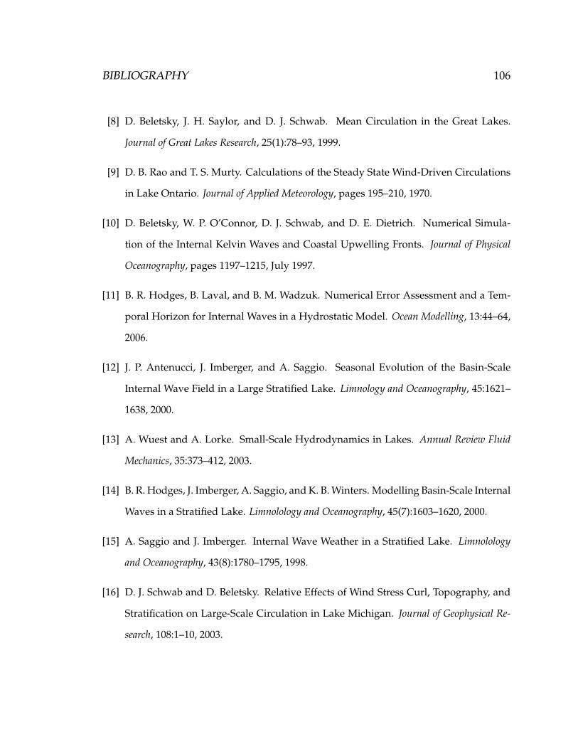
BIBLIOGRAPHY 106
[8] D. Beletsky, J. H. Saylor, and D. J. Schwab. Mean Circulation in the Great Lakes.
Journal of Great Lakes Research, 25(1):78–93, 1999.
[9] D. B. Rao and T. S. Murty. Calculations of the Steady State Wind-Driven Circulations
in Lake Ontario. Journal of Applied Meteorology, pages 195–210, 1970.
[10] D. Beletsky, W. P. O’Connor, D. J. Schwab, and D. E. Dietrich. Numerical Simula-
tion of the Internal Kelvin Waves and Coastal Upwelling Fronts. Journal of Physical
Oceanography, pages 1197–1215, July 1997.
[11] B. R. Hodges, B. Laval, and B. M. Wadzuk. Numerical Error Assessment and a Tem-
poral Horizon for Internal Waves in a Hydrostatic Model. Ocean Modelling, 13:44–64,
2006.
[12] J. P. Antenucci, J. Imberger, and A. Saggio. Seasonal Evolution of the Basin-Scale
Internal Wave Field in a Large Stratified Lake. Limnology and Oceanography, 45:1621–
1638, 2000.
[13] A. Wuest and A. Lorke. Small-Scale Hydrodynamics in Lakes. Annual Review Fluid
Mechanics, 35:373–412, 2003.
[14] B. R. Hodges, J. Imberger, A. Saggio, and K. B. Winters. Modelling Basin-Scale Internal
Waves in a Stratified Lake. Limnolology and Oceanography, 45(7):1603–1620, 2000.
[15] A. Saggio and J. Imberger. Internal Wave Weather in a Stratified Lake. Limnolology
and Oceanography, 43(8):1780–1795, 1998.
[16] D. J. Schwab and D. Beletsky. Relative Effects of Wind Stress Curl, Topography, and
Stratification on Large-Scale Circulation in Lake Michigan. Journal of Geophysical Re-
search, 108:1–10, 2003.

BIBLIOGRAPHY 107
[17] G. T. Csanady. Hydrodynamics of Large Lakes. Technical Report 3340, Woods Hole
Oceanographic Institution, 1975.
[18] Robert G. Wetzel. Limnology: Lake and River Ecosystems. London: Academic, SanDiego,
California, third edition, 2001.
[19] B. Laval, J. Imberger, B. R. Hodges, and R. Stocker. Modelling Circulation in Lakes:
Spatial and Temporal Variations. Limnolology and Oceanography, 48(3):983–994, 2003.
[20] J. R. Bennett. A Three-Dimensional Model of Lake Ontario’s Summer Circulation I.
Comparison with Observations. Journal of Physical Oceanography, 7:591–601, 1977.
[21] R. H. Spigel and J. Imberger. The Classification of Mixed-Layer Dynamics in Lakes of
Small to Medium Size. Journal of Physical Oceanography, 10:1104–1121, 1980.
[22] C. H. Mortimer. Lake hydrodynamics. Mitteilugen der internaltionale Vereinigung fur
theoretische und angewandte Limnologie, 20:124–197, 1974.
[23] T. J. Simons, C. R. Murthy, and J. E. Campbell. Winter Circulation in Lake Ontario.
Journal of Great Lakes Research, 11:423–433, 1985.
[24] R. L. Pickett. The Observed Winter Circulation of Lake Ontario. Journal of Physical
Oceanography, 7:152–156, 1977.
[25] A. E. Gill. Atmosphere-Ocean Dynamics, volume 30 of International Geophysics Series.
Academic Press, New York, 1982.
[26] D. J. Schwab. Internal Free Oscillations in Lake Ontario. Limnology and Oceanography,
22(4):700–708, July 1977.
[27] G. T. Csanady. The Coastal Boundary Layer in Lake Ontario: Part II. The Summer-Fall
Regime. Journal of Physical Oceanography, pages 168–176, 1972.
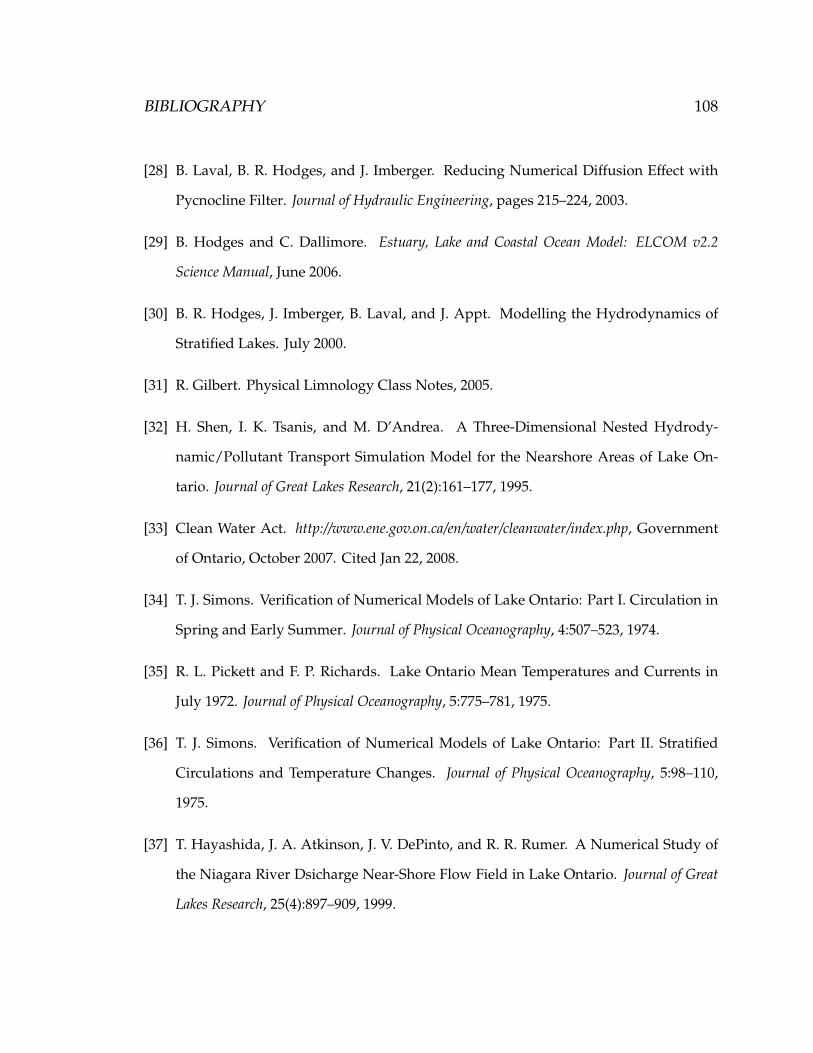
BIBLIOGRAPHY 108
[28] B. Laval, B. R. Hodges, and J. Imberger. Reducing Numerical Diffusion Effect with
Pycnocline Filter. Journal of Hydraulic Engineering, pages 215–224, 2003.
[29] B. Hodges and C. Dallimore. Estuary, Lake and Coastal Ocean Model: ELCOM v2.2
Science Manual, June 2006.
[30] B. R. Hodges, J. Imberger, B. Laval, and J. Appt. Modelling the Hydrodynamics of
Stratified Lakes. July 2000.
[31] R. Gilbert. Physical Limnology Class Notes, 2005.
[32] H. Shen, I. K. Tsanis, and M. D’Andrea. A Three-Dimensional Nested Hydrody-
namic/Pollutant Transport Simulation Model for the Nearshore Areas of Lake On-
tario. Journal of Great Lakes Research, 21(2):161–177, 1995.
[33] Clean Water Act. http://www.ene.gov.on.ca/en/water/cleanwater/index.php, Government
of Ontario, October 2007. Cited Jan 22, 2008.
[34] T. J. Simons. Verification of Numerical Models of Lake Ontario: Part I. Circulation in
Spring and Early Summer. Journal of Physical Oceanography, 4:507–523, 1974.
[35] R. L. Pickett and F. P. Richards. Lake Ontario Mean Temperatures and Currents in
July 1972. Journal of Physical Oceanography, 5:775–781, 1975.
[36] T. J. Simons. Verification of Numerical Models of Lake Ontario: Part II. Stratified
Circulations and Temperature Changes. Journal of Physical Oceanography, 5:98–110,
1975.
[37] T. Hayashida, J. A. Atkinson, J. V. DePinto, and R. R. Rumer. A Numerical Study of
the Niagara River Dsicharge Near-Shore Flow Field in Lake Ontario. Journal of Great
Lakes Research, 25(4):897–909, 1999.

BIBLIOGRAPHY 109
[38] Centre for Water Research, University of Western Australia : ELCOM.
http://www.cwr.uwa.edu.au/research/publications.php?title=&keywords=ELCOM&author=
&ED Number=&type=Journal&publication status=Published&year from=&year to=&search=
Search.
[39] R. S. Gupta. Hydrology and Hydraulic Systems. Waveland Press, Inc., Long Grove,
Illinois, second edition, 2001.
[40] L. F. Leon, D. Lam, W. Schertzer, and D. Swayne. Lake and Climate Models Linkage:
a 3-D Hydrodynamic Contribution. Advances in Geosciences, 4:57–62, 2005.
[41] D. J. Schwab and D. L. Sellers. Great Lakes Bathymetry and Shoreline Data.
http://www.glerl.noaa.gov/data/bathy/bathy.html, Great LakesEnvironmental Reseach
Laboratory, National Atmospheric Administration.
[42] B. Hodges and C. Dallimore. Estuary, Lake and Coastal Ocean Model: ELCOM v2.2 User
Manual, February 2007.
[43] I. K. Tsanis and C. R. Murthy. Flow Distribution in the St. Lawrence River System at
Wolf Island, Kingston Basin, Lake Ontario. Journal of Great Lakes Research, 16(3):352–
365, 1990.
[44] Lake Ontario, Physical and Environmental Features of the Lake Ontario Basin.
http://epa.gov/greatlakes/ontario.html, U.S. Environmental Protection Agency, Novem-
ber 2007. Cited March 21, 2008.
[45] Historic Great Lakes Water Level Data - Station Selection.
http://tidesandcurrents.noaa.gov/station retrieve.shtml?type=Historic+Great+Lakes+Water+
Level+Data, National Oceananic and Atmospheric Association, 2006.

BIBLIOGRAPHY 110
[46] TidbiT Data Logger. http://www.microdaq.com/occ/other/tidbit data logger.php, TheData-
LoggerStore.com, 2008.
[47] SC-ADCP Technical Manual - Appendix S: Spcifications and Dimentions. Burlington, ON,
1991.
[48] L. F. Leon. Lake Ontario 3D Modelling. http://www.science.uwaterloo.ca/ lfleonvi/ontmodel/
lakemodel main.html, University of Waterloo, 2008.
[49] B. K. Pal, R. Murthy, and R. E. Thomson. Lagrangian Measurements in Lake Ontario.
Journal of Great Lakes Research, 24(3):681–697, 1998.
[50] B. Hodges. Numerical Techniques in CWR-ELCOM (code release v.1), March 2000.
Appendix A
Scaled vs Non-Scaled Temperature
Profiles
Over course of several ELCOM simulations, it was found that both long and shortwave
radiation as well as air temperature, are the most important factors influencing the tem-
perature of the modelled water body. Because ELCOM has a tendency to underestimate
water temperatures, both the long and shortwave radiation values were scaled by 1.15 and
0.9 respectively as was done by Laval et al. for Lake Kinneret simulations to improve mod-
elled results [28]. Figures A.1, A.2, A.3 and A.4 compare unscaled and scaled radiation
ELCOM results with observed temperatures. Scaled temperature profile results portray
overall warmer water than unscaled data. Although scaled results are still cooler than
observed, they compare better than unscaled results.
111

APPENDIX A. SCALED VS NON-SCALED TEMPERATURE PROFILES 112
Figure A.1: Unscaled (a) versus scaled (b) ELCOM simulated temperature profilescompared with observed data (c) at station 1263.

APPENDIX A. SCALED VS NON-SCALED TEMPERATURE PROFILES 113
Figure A.2: Unscaled (a) versus scaled (b) ELCOM simulated temperature profilescompared with observed data (c) at station 586.

APPENDIX A. SCALED VS NON-SCALED TEMPERATURE PROFILES 114
Figure A.3: Unscaled (a) versus scaled (b) ELCOM simulated temperature profilescompared with observed data (c) at station 403.

APPENDIX A. SCALED VS NON-SCALED TEMPERATURE PROFILES 115
Figure A.4: Unscaled (a) versus scaled (b) ELCOM simulated temperature profilescompared with observed data (c) at station 1266.

Appendix B
Water Levels
The first lake-wide numerical models were closed basin models, not accounting for water
flow in and out of the lake, or models having constant inflow and outflow effectively can-
celing out this term in the water balance equation [5, 34, 36]. At such coarse grid scales it
was thought that inflows and outflows would not significantly impact the model results.
However, with the large volume of water in lakes the size of the Great Lakes, inflows and
outflows can significantly impact water volumes in ELCOM simulations. Newer models
such as the ELCOM model of Lake Erie includes major inflows and outflows [6]. Using as
many available data sources as possible when evaluating the performance of a lake-wide
model is preferred to be certain that simulations are properly reproducing observed lake
hydrodynamics. ELCOM was compared to observed thermistor chain data, current meter
data and historic water level data. Both simulated temperatures and currents compared
well for ELCOM models of Lake Erie and Lake Kinneret [6, 14]. When evaluating ELCOM
water levels for Lake Ontario, it became obvious that the lake’s water balance was very im-
portant in order to be sure that the model properly represented all the lake’s hydrodynamic
processes. The model was first run as a closed basin as seen in Figure B.1. The difference
between simulated and observed hourly water level fluctuations in Figure B.1 exemplifies
116
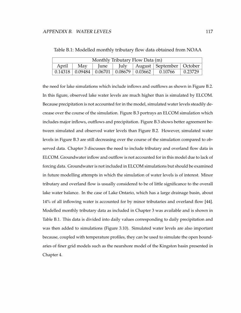
APPENDIX B. WATER LEVELS 117
Table B.1: Modelled monthly tributary flow data obtained from NOAA
Monthly Tributary Flow Data (m)April May June July August September October
0.14318 0.09484 0.06701 0.08679 0.03662 0.10766 0.23729
the need for lake simulations which include inflows and outflows as shown in Figure B.2.
In this figure, observed lake water levels are much higher than is simulated by ELCOM.
Because precipitation is not accounted for in the model, simulated water levels steadily de-
crease over the course of the simulation. Figure B.3 portrays an ELCOM simulation which
includes major inflows, outflows and precipitation. Figure B.3 shows better agreement be-
tween simulated and observed water levels than Figure B.2. However, simulated water
levels in Figure B.3 are still decreasing over the course of the simulation compared to ob-
served data. Chapter 3 discusses the need to include tributary and overland flow data in
ELCOM. Groundwater inflow and outflow is not accounted for in this model due to lack of
forcing data. Groundwater is not included in ELCOM simulations but should be examined
in future modelling attempts in which the simulation of water levels is of interest. Minor
tributary and overland flow is usually considered to be of little significance to the overall
lake water balance. In the case of Lake Ontario, which has a large drainage basin, about
14% of all inflowing water is accounted for by minor tributaries and overland flow [44].
Modelled monthly tributary data as included in Chapter 3 was available and is shown in
Table B.1. This data is divided into daily values corresponding to daily precipitation and
was then added to simulations (Figure 3.10). Simulated water levels are also important
because, coupled with temperature profiles, they can be used to simulate the open bound-
aries of finer grid models such as the nearshore model of the Kingston basin presented in
Chapter 4.

APPENDIX B. WATER LEVELS 118
Figure B.1: Observed and simulated hourly water level fluctuations for a closedbasin simulation.

APPENDIX B. WATER LEVELS 119
Figure B.2: Observed and simulated hourly water level fluctuations. Simulationincludes major inflows from the Niagara River and Welland canal aswell as outflow from the St. Lawrence River.
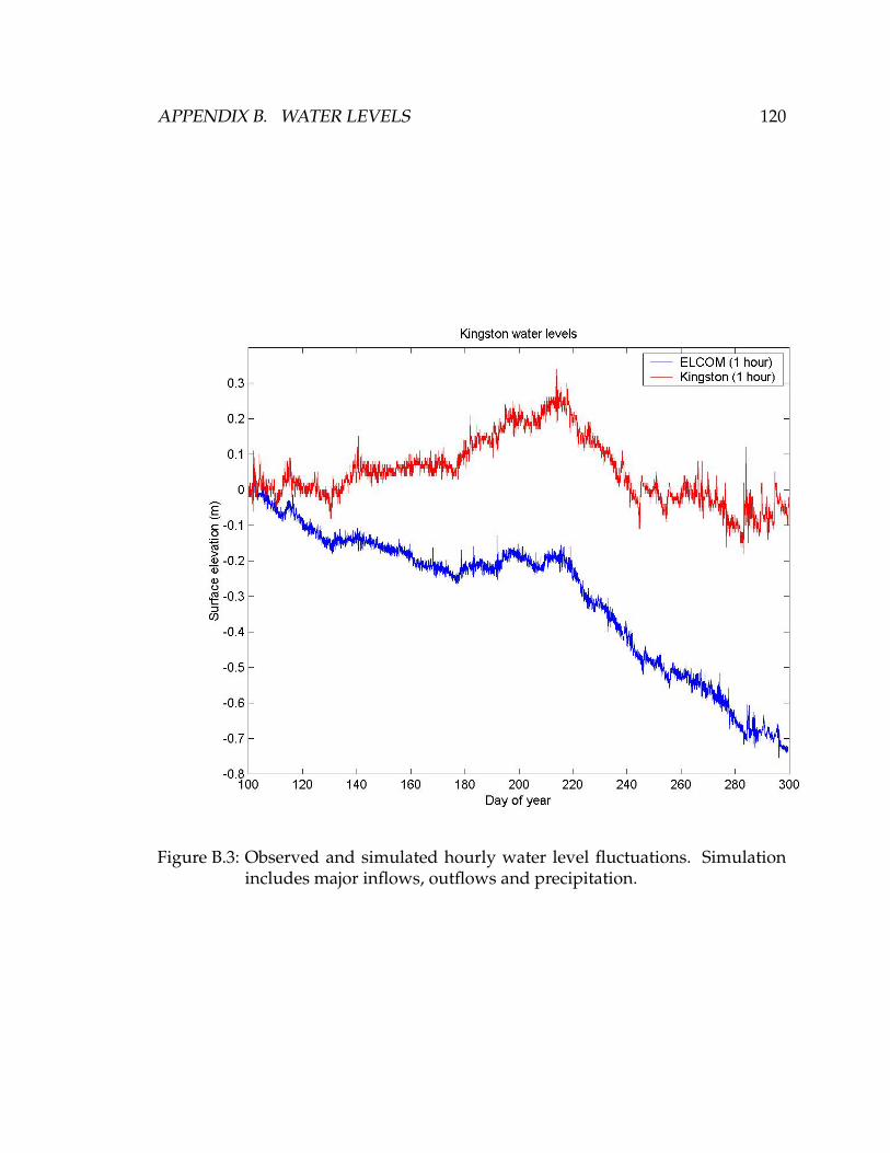
APPENDIX B. WATER LEVELS 120
Figure B.3: Observed and simulated hourly water level fluctuations. Simulationincludes major inflows, outflows and precipitation.
Appendix C
Lake-Wide Current Comparisons
A lake-wide current plot is presented in Chapter 3 in comparison to Beletsky et al.’s plot
of general summer circulation. This plot was computed using ELCOM current results at
depths of 15, 19, 30, 50 and 75 m. Figure C.1 demonstrates the depth averaged ELCOM
simulated circulation in all of Lake Ontario for the entire length of the 2006 simulation.
This figure is the best representation of the model’s performance. Further current compar-
isons with literature are discussed below.
Prakash et al. used a PTM to study surface circulation and noted a coastal current along
the southern shore east of the Niagara River and a clockwise gyre in the Rochester basin
in August [5]. Surface simulated summer coastal currents are reproduced throughout the
ELCOM simulation shown in Figure C.2.
The gyre in the Rochester basin seen in the August simulation of surface currents in
Prakash et al. is not as pronounced in the ELCOM 2006 August simulation results (Figure
C.3), instead there is a small clockwise gyre coupled with a another small anticlockwise
gyre directly to the north. This discrepancy can be attributed to interannual variability.
ELCOM May 2006 surface circulation in Figure C.4 generally compares well to May
circulation patterns seen in Prakash et al. with the exception of the coastal current along
121

APPENDIX C. LAKE-WIDE CURRENT COMPARISONS 122
Figure C.1: Lake-wide ELCOM simulated summer depth averaged currents inLake Ontario.
the south shore which is less evident in the ELCOM simulation.
For comparison to Pal et al. [49], ELCOM mean summer currents at a depth of 3.5 m
were plotted in Figure C.5. The counterclockwise gyre in the south-western part of the lake
as seen in Pal et al. is well reproduced by ELCOM along with the south coastal current.
The gyre portrayed in Pal et al. in the north part of the lake [49] is not reproduced by the
ELCOM simulation. This could be due to seasonal variations or insufficient drifter data.
However, more analysis would be required to further comment on this but is beyond the
scope to this project. ELCOM can be used to model the release of drifters to simulate the
studies described in Pal et al. which would give a more comprehensive comparison.
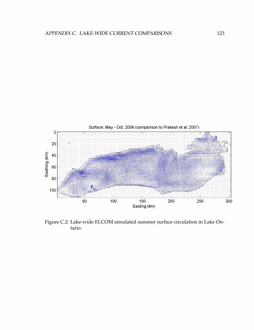
APPENDIX C. LAKE-WIDE CURRENT COMPARISONS 123
Figure C.2: Lake-wide ELCOM simulated summer surface circulation in Lake On-tario.

APPENDIX C. LAKE-WIDE CURRENT COMPARISONS 124
Figure C.3: Lake-wide ELCOM simulated surface currents for August 2006 in LakeOntario.

APPENDIX C. LAKE-WIDE CURRENT COMPARISONS 125
Figure C.4: Lake-wide ELCOM simulated surface currents for May 2006 in LakeOntario.

APPENDIX C. LAKE-WIDE CURRENT COMPARISONS 126
Figure C.5: Lake-wide ELCOM simulated currents at a depth of 3.5 m in Lake On-tario.
Appendix D
ELCOM Transport Equations
ELCOM transport equations (Figure D.1) and nomenclature (Figure D.2) are shown below
as found in literature.
127

APPENDIX D. ELCOM TRANSPORT EQUATIONS 128
Figure D.1: ELCOM equations as found in literature [50]

APPENDIX D. ELCOM TRANSPORT EQUATIONS 129
Figure D.2: ELCOM nomenclature as found in literature [50]

Appendix E
Velocity Difference
The absolute difference between ELCOM and observed north-south and east-west compo-
nents of velocity was plotted for the coarse grid lake-wide model presented in Chapter 3
at station 1263 (Figure E.1) and station 1266 (Figure E.2). Figure E.1 shows both compo-
nents of velocities to compare similarly. Both components of velocity show discrepancies
between modelled and observed data mostly between 0 and 10 cm/s. Larger deficiencies
occur periodically and are shown in both components of velocity. Figure E.2 first portrays
the north-south component of velocity to agree well with observed values as discrepancies
are between 0 and 4 cm/s for water in the hypolimnion. The water in the top portion of the
profile shows slightly larger discrepancies in velocity especially around day 250 at the time
of the storm event discussed in Chapter 3. The simulated east-west component of velocity
at this location agrees less with with observed values than the north-south component and
around the time of the storm event (day 250) where discrepancies between the modelled
and observed velocities is very high.
The absolute difference between ELCOM and observed north-south and east-west com-
ponents of velocity was plotted for the nearshore model of the Kingston basin and the
upper portion of the St. Lawrence River presented in Chapter 4 at station 1263 (Figures
130

APPENDIX E. VELOCITY DIFFERENCE 131
E.3 and E.4). Figure E.3 shows similar velocity discrepancies in the north-south direction
for simulations A and B. Larger discrepancies are shown to occur in the top half portion of
these two profiles. Discrepancies in the comparison of modelled and observed north-south
components of velocity for simulation C are shown to be much larger throughout most of
the water column especially in the second half of the simulation. Figure E.4 portrays again
similar discrepancies in the east-west component of velocity for simulations A and B. The
first half of the these two profiles show smaller discrepancies than is seen in the north-
south component of velocity. However the second half of the simulation shows larger
discrepancies in than is seen with the east-west component. The east-west component of
velocity for simulation C again shows much larger velocity discrepancies than simulations
A or B, but smaller discrepancies than is seen in the north-south component of velocity for
simulation C.

APPENDIX E. VELOCITY DIFFERENCE 132
Figure E.1: Coarse grid model velocity difference. Absolute difference betweenELCOM daily velocities and observed daily velocities in cm/s at 1 mdepth intervals. North-south component of velocity difference (a) andthe east-west component of velocity (b).

APPENDIX E. VELOCITY DIFFERENCE 133
Figure E.2: Coarse grid model velocity difference. Absolute difference betweenELCOM daily velocities and observed daily velocities in cm/s at 2 mdepth intervals. North-south component of velocity difference (a) andthe east-west component of velocity (b).

APPENDIX E. VELOCITY DIFFERENCE 134
Figure E.3: Nearshore model north component of velocity difference at station1263. Absolute difference between ELCOM daily velocities and ob-served daily velocities in cm/s at 1 m depth intervals. North-southcomponent of velocity difference for simulation A (a), simulation B (b)and simulation C (c).

APPENDIX E. VELOCITY DIFFERENCE 135
Figure E.4: Nearshore model east component of velocity difference at station 1263.Absolute difference between ELCOM daily velocities and observeddaily velocities in cm/s at 1 m depth intervals. East-west component ofvelocity difference for simulation A (a), simulation B (b) and simulationC (c).