hydrodynamic and chemical modelling of the baltic sea

7.0 9.0 11.0 13.0 15.0 17.0 19.0 21.0 23.0 25.0 27.0

Merentutkimuslaitos Havsforskningsinstitutet

Finnish Institute of Marine Research

HYDRODYNAMIC AND CHEMICAL MODELLING OF THE BALTIC SEA - A THREE-DIMENSIONAL APPROACH

Oleg Andrejev, Kai Myrberg, Alexander Andrejev and Matti Perttilä

MERI - Report Series of the Finnish Institute of Marine Research No. 42, 2000

HYDRODYNAMIC AND CHEMICAL MODELLING OF THE BALTIC SEA —A THREE-DIMENSIONAL APPROACH

Oleg Andrejev, Kai Myrberg, Alexander Andrejev and Matti Perttilä

MERI — Report Series of the Finnish Institute of Marine Research No. 42, 2000

Cover photo: Simulated bottom salinity of the Baltic Sea on August 31, 1987.

Publisher: Finnish Institute of Marine Research P.O. Box 33 FIN-00931 Helsinki, Finland Tel: + 358 9 613941 Fax: + 358 9 61 394 494 e-mail: [email protected]

Julkaisija: Merentutkimuslaitos PL 33 00931 Helsinki Puh: 09-613941 Telekopio: 09-61394 494 e-mail: sukunimi @fimr.fi

Copies of this Report Series may be obtained from the library of the Finnish Institute of Marine Research.

Tämän raporttisarjan numeroita voi tilata Merentutkimuslaitoksen kirjastosta.

ISSN 1238-5328 ISBN 951-53-2184-0

HYDRODYNAMIC AND CHEMICAL MODELLING OF THE BALTIC SEA A THREE-DIMENSIONAL APPROACH

Oleg Andrejev', Kai Myrberg2*, Alexander Andrejev' and Matti Perttilä'

' Finnish Institute of Marine Research P.O. Box 33, FIN-00931 Helsinki, Finland

2 Department of Meteorology, University of Stockholm, S-106 91, Stockholm, Sweden

* on leave from the Finnish Institute of Marine Research

ABSTRACT

A modelling system for the Baltic Sea has been developed based on the use of a data assimilation system (DAS), which is coupled with the Baltic Environmental Database and with a three-dimensional baroclinic prognostic model. The basic model equations and the development of a user-friendly interface are described. In this paper the model is applied in studies of the basic hydrodynamic features of the Baltic Sea, e.g. the mean circulation and its stability, water exchange and related features, the horizontal and vertical structure of salinity, sea-level variations and upwellings, and sea temperature. A chemical model is used to investigate the sediment-water interface processes. A nested grid system is utilised throughout the simulations, in which a horizontal resolution of one nautical mile is used in the area of interest.

Keywords: three-dimensional approach, hydrodynamic modelling, chemical modelling, user-friendly interface

1. INTRODUCTION

Many three-dimensional model systems for the Baltic Sea have already been developed in various institutions, and a large number of applications have been tested. Some of the models are especially devoted to studies of the hydrodynamics, but often an ecosystem-oriented strategy is used instead. This paper describes the further development of, and new results from, a system in which construction of the database, analysis of the data as well as the modelling itself have been coupled with each other from the beginning. In particular, the Data Assimilation System DAS (Sokolov & al. 1997) coupled with the Baltic Environmental Database (BED) (Wulff & Rahm, 1991) and a three-dimensional hydrodynamic model (Andrejev & Sokolov, 1989; Andrejev & Sokolov, 1992; Engqvist & Andrejev, 1999) as an interpolation tool, is an attempt to construct a public information system to work with Baltic Sea oceanographic data.

This three-dimensional modelling system is applied especially to studies of the Baltic Proper and Gulf of Finland. A nested grid system is used in which a high horizontal resolution (usually one nautical mile) is used in the area of interest, while the other parts of the Baltic Sea are modelled with a coarser grid. Both hydrodynamic and chemical modelling is carried out, and the results of the simulations are discussed in this report.

The Baltic Sea is a shallow brackish-water basin, permanently stratified and therefore subject to redox variations. The water exchange with the adjacent North Sea is restricted, and in consequence, sedimentation and sediment processes play an important role in the mass balance estimations of the Baltic Sea. Nutrient regeneration in the sediments constitutes an important feedback link in closing the nitrogen and phosphorus biogeochemical cycles. Knowledge of the interactions between pelagic and sediment sub-systems is also essential for nutrient budget calculations and turnover time estimates on the basin-wide long-term scales in both empirical and simulation ecosystem models (Wulff & al. 1990; Savchuk & Wulff, 1996). Sediment description is thus an inherent part of modern aquatic ecosystem models (Baretta & al. 1995; Ruardij & Van Raaphorst, 1995; Tamsalu & Ennet 1995).

4 Oleg Andrejev, Kai Myrberg, Alexander Andrejev and Matti Perttilä MERI No. 42, 2000

Sediment processes are usually quantified by means of two different approaches or their combination. The "Direct" approach is based on measurements during laboratory or in situ incubations of core tubes or benthic chambers, sometimes artificially enriched with algal material (see e.g. Balzer, 1984; Conley & Johnstone, 1995; Hall & al. 1996; Tuominen & al. 1999). The "Inverse " approach involves either simple flux calculations based on observed concentration gradients at the sediment-water interface (see e.g. Hall & al. 1996; Lehtoranta, 1998) or more sophisticated fitting of the sediment models to observed vertical profiles (see e.g. Van Raaphorst & al. 1990; Jensen & al. 1994).

In spite of the importance of sediment processes and the potential existing for their quantification, there is a surprisingly small number of studies of sediment processes in the Baltic Sea, and these are mainly on the nutrient water-bottom exchange (Koop & al. 1990; Conley & al. 1997; Lehtoranta, 1998, and references in these sources). Many uncertainties also remain in current estimates due to the methodological and analytical difficulties encountered in implementation of different schemes of measurements and calculations (Stockenberg, 1998). Further, the irregular mosaic distribution of different sediment types and sparse sampling also hamper accurate interpolations to a basin-wide scale, even when using reliable site estimates. Finally, nutrient concentrations in the pore water, needed in the "inverse" approach for flux calculations, have been sampled far more seldom than the nutrient content of the sediment solid phase. The intention of the present study is to develop a model of the coupled nitrogen and phosphorus sediment processes in order to provide a tool to estimate the main transport and transformation fluxes from given vertical distributions of organic matter.

In the hydrodynamic modelling, the main interest lies in the simulations of the Gulf of Finland. The gulf is an interesting sub-area of the Baltic Sea because of its complicated hydrographic nature. The western end of the gulf is a direct continuation of the Baltic Sea Proper, whereas the eastern end of the gulf receives the largest single fresh water input to the whole Baltic Sea, namely the River Neva, with a mean input of about 2700 m3/s. This leads to a continuous east-west salinity gradient in the gulf. The stratification conditions are very variable in space and time for the above-mentioned reasons and because of the large seasonal variations in incoming solar radiation. The density-driven circulation is an important factor in modifying currents in the gulf, in addition to the wind forcing and the forcing introduced by the surface slope. The hydrographic features are strongly modified by the variable and complex bottom topography as well. The hydrodynamics of the gulf is described in detail by Alenius & al. (1998). Many basic features are simulated here: sea-level variations, mean circulation conditions, water exchange with the Baltic Sea Proper, renewal time of the gulf water, and salinity structure, as well as upwelling dynamics and related changes in temperature. The background of these different physical processes is discussed too.

Among the hydrodynamically-oriented three-dimensional model systems developed for the Baltic Sea area the following approaches can be mentioned. Simons (1976, 1978) applied his model to the Baltic Sea and studied the role of topography, stratification and boundary conditions in the wind-driven circulation. Kielmann (1981) continued the studies of currents and water levels using Simons' model. Funkquist & Gidhagen (1984) have applied Kielmann's model version. Krauss & Brügge (1991), Elken (1994) and Lehmann (1995) have applied the Bryan-Cox-Semtner-Killworth free-surface model version (Killworth & al. 1991) for studying various aspects of the physics of the Baltic Sea. Fennel & Neumann (1996) have studied the meso-scale current patterns in the southern Baltic using the MOM 1 (MOM=Modular Ocean Model) version of the Bryan-Cox model with a horizontal resolution of one nautical mile. Klevanny (1994) has developed a modelling system of two-and three-dimensional models for studying various water bodies: rivers, lakes and seas (including the Baltic Sea). Tamsalu & Ennet (1995), Tamsalu & Myrberg (1995) and Tamsalu (1998) have developed a coupled hydrodynamic-ecological model for the Baltic Sea especially focused on studies of the Gulf of Finland and Gulf of Riga. Meier & al. (1999) have applied the Bryan-Cox-Semtner-Killworth free-surface version to Baltic Sea climate studies.

This report is organised as follows: First, the main model equations, both physical and chemical, will be introduced. In the third section, the user-friendly interface is introduced. The fourth section is devoted to describing the material and methods used. In the fifth section the latest model results are presented and analysed. At the end, a summary is given, including some ideas for future work.

Hydrodynamic and chemical modelling of the Baltic Sea — a three-dimensional modelling approach 5

2. THE MODEL EQUATIONS

The numerical model used in the present study was formulated by Andrejev & Sokolov (1989, 1990). A comprehensive description of the equations including the numerical algorithms can be found in Sokolov & al. (1997). The model may be characterised as a time-dependent, free-surface, baroclinic three-dimensional model. The usual simplifications in the form of the hydrostatic approximation, the incompressibility condition, the Laplacian closure hypothesis for subgridscale turbulent mixing, and the traditional approximation for the Coriolis force are made. It is also assumed that density variations are only manifested in the buoyancy terms. Elsewhere the density is taken to be constant.

2.1 The general equations

The governing equations of the model are:

du duu duv duw 1 ap d

l ~ atr.

~t+ ~

+ ay + az —~— Po ax+pAu+ rh V az (1)

av + avu + avv + avw = — fic — 1 ap + µ0v + a v av at ax ay az Po ay az az

du åv arv —dx +—ay + az

=0

p= p(T, S)

~= Pg

ax auX avX awX µ

( ax) t at + ax + ay + az = oX+azl az J +F

The first two of this set of basic equations denote the momentum balances in the x-and y-direction respectively (x increases eastwards, y increases northwards). The velocities in the horizontal direction are u in the x-direction and v in the y-direction. In the vertical direction (z increasing downwards) the velocity is denoted by w. Pressure has the symbol p and Po is a reference density (1000 kg/m3).

The kinematic eddy diffusivity coefficients in the horizontal and vertical directions are and v. The former is set to be constant at 50 m2/s for the Baltic Sea Proper and 30 m2/s for the Gulf of Finland, but the latter varies with depth, and is made dependent on the local vertical shear and buoyancy forces in accordance with Marchuk (1980). Finally f is the Coriolis-parameter, taking into account the effect of the earth's rotation. All other external forces, such as wind stress and bottom friction are entered in the form of boundary conditions. The horizontal Laplacian operator is denoted A.

a2 d2 A= dx2 + dy2

Equation (3) is the volume conservation equation. The actual small compressibility of water is neglected, which introduces a negligible mass conservation error. The state equation (4) thus also reflects the absence of depth dependence and has been adopted from Millero & Kremling (1976).


Equation (5) takes full account of the vertical density variations, which are not reflected in equations (1) and (2). This is often referred to as the Boussinesqian hydrostatic approximation. The gravitational acceleration is denoted by g (m/s2). In equation (6) X denotes the concentration of the modelled scalar properties that enter (or exit) the model boundaries or have sources (or sinks), denoted F, within the model domain. These scalars are salinity (S), heat (pCPT; where Cp is the specific heat of water and T is the temperature) or the "age" A). The last item of this trio denotes the volume-specific transit retention time (Bohlin & Rodhe, 1973) with the physical dimension of days/m3.

The parameterization of the vertical eddy diffusivity coefficient v is taken from Marchuk (1980):

v =(0.05h)2 a11 ~ av

2 g ap

( az ~ +~ az~ Po az (7)

The parameter h is set as 2.5 m.

2.2 Model parameterizations

The drag coefficient Cd at the sea-surface is taken from Bunker (1977):

Cd =0.0012( W 0.066+0.63)

(8)

where:

W is the wind velocity (m/s). For the bottom friction, Cdb was set to 0.0026.

The formulation of heat transfer at the air-sea interface (Lane & Prandle, 1996) is given as:

5.10-6 +3.10-6 (T~,-TS ) FT = ~ Ot

1 (9)

where:

Ta is the air temperature, T, is the sea-surface temperature, Azl is the thickness of the top layer. For salinity the corresponding flux F, is set, as a first approximation, to equal zero.

The solid vertical walls are prescribed to be of a non-slip type. Neither these nor the bottom bed are designed to be permeable to the scalar properties, except for the locations where the rivers discharge. At these places the salinity is set to zero, while the river water instantaneously adapts to the temperature of the ambient water. The open boundary conditions are described in section 4.

The ice dynamics have been formulated in a simple way: at water temperatures below -0.2°C the wind stress is lowered by a factor of 10 and at 0.0 °C the heat flux through the ice is shut off as long as cooling conditions prevail. The reason for not reducing the wind stress completely is so that the wind set-up mechanism, by tilting the ice-covered surface, remains. No ice drift mechanism is therefore modelled either.

Finally, there is also a kinematic boundary condition that expresses that a fluid particle on the surface remains there regardless of the advective motion of the underlying layers.

2.3 Numerical methods

The whole Baltic Sea model consists of 18 vertical levels with irregular vertical spacing and with a monotonically increasing layer thickness toward the bottom. The depths of the layer interfaces are: 0 m, 2.5 m, 7.5 m, 12.5 m, 17.5 m, 22.5 m, 27.5 m, 35.0 m, 45.0 m, 55.0 m, 65.0 m, 75.0 m, 85.0 m, 95.0 m, 105.0 m, 137.5 m, 162.5 m, 187.5 m and the bottom. In the Gulf of Finland, the three last layers do not exist.


A comprehensive description of the numeric scheme and other model constructs have been given in detail by Sokolov & al. (1997). Here, only a brief description of the main features is introduced. The equations are given in flux form to insure that certain integral constraints are maintained by the differentiation (Blumberg & Mellor, 1987). The finite difference approximation of the model equations is constructed by integrating them over the C-grid (Mesinger & Arakawa, 1976) cell volume. The time step was split up as suggested by Liu & Leendertse (1978). Thus, the u-equations are solved at time steps n-1/2 — n+l/2 (n denotes a time step number), the v-equations are solved at the time steps n — n+1, and all the other equations are solved at every half time step. All vertical derivatives and bottom friction were treated implicitly. A technique, known as mode splitting (Simons, 1974), was used. The two-dimensional equation for the volume transport (external mode) is obtained by summation of finite difference approximations of three-dimensional momentum equations over the vertical direction. Before the three-dimensional finite difference equations (internal mode) can be solved, the sea-surface elevation is calculated from the volume transport equation and from the vertically-integrated equation of continuity.

A bottom frictional stress enters semi-implicitly into both modes and uses a bottom layer velocity that has to be calculated. This treatment of the bottom friction is realised numerically in the framework of an iterative procedure. Thus, the two-dimensional and three-dimensional momentum equations are solved repeatedly until the absolute value of the maximum difference between the bottom velocities and neighbouring iterations become less than some small positive number. This adjustment allows the use of an alternation direction implicit method for solving the volume transport equation (Liu & Leendertse, 1978; Andrejev & Sokolov, 1989) and the adoption of the same time step for the two-dimensional as well as for the three-dimensional parts of the model. It should be noted that the Gaussian elimination method makes it possible to solve these quite easily.

2.4 Vertical convection

The vertical convection has to parameterised, since the model uses the hydrostatic approximation. The following heuristic algorithm is used. Firstly, a check is made whether the water in a grid cell is in a stable state relatively to the water of the lower cell. If it is not, then the water of the unstable grid cell (or some part of it) is moved into the lower cell and the same volume of water from the lower cell is displaced upwards and mixed here with the upper cell water. This procedure of downward water replacement proceeds cell by cell until the sinking volume finds itself in a stable state. At this point the sinking volume is well-mixed. The whole procedure starts from the lowest two cells.

2.5. The chemical model

The model state variables are ammonium A, nitrate N, phosphate P, and oxygen 0. The dynamics of the vertical distribution of these substances is described by a system of general one-dimensional diagenetic equations under the following assumptions: a) an adsorption is approximated with the Freundlich adsorption equilibrium, b) the pore water advection is insignificant comparing to other processes concerned, c) the rates of deposition and compaction are constant, i.e. the porosity profile preserves its shape (Lerman, 1977; Berner, 1980):

aCi = 1 a (K1+1) at 13, az aci (1)Di — Ri + Si (10) az

with the boundary conditions:

z=0; Ci = Co,i (11)

z (12)


In Eqs. 11 — 12: C,(z) (mmol m 3) is the concentration of the i-th substance (i = 1...4, C, = A, N, P, 0, respectively) dissolved in the pore water; the vertical distance co-ordinate z (metres) is given as z = 0 at the sediment-water interface, increasing downwards; t (day) is time; 0(z) is the vertical distribution of porosity (volume fraction of sediment occupied by water); D; (m2 d-1) is the effective diffusion coefficient of the substance in the pore water; R, and Si (mmol m3 d-1) are removal and supply rates, K, is a dimensionless distribution coefficient defined as the proportion between the concentrations of the absorbed and dissolved phases; Co,, is a given concentration at the sediment-water interface.

All removal processes are treated as first-order chemical reactions, while supply processes are assumed to have zero-order kinetics, and fast adsorption is considered to be an instantaneous equilibrium reaction (Lerman, 1977; Seitzinger, 1990; Ruardij & Van Raaphorst, 1995). The diffusion flows for all species are set equal to zero at the lower boundary.

To create the diagenetic equations for each substance under consideration we assume that:

Ammonium is produced by mineralization of organic nitrogen, its losses being caused by nitrification, which only takes place under oxic conditions, while in anoxic conditions a certain part is adsorbed onto sediment particles.

Nitrate is produced by nitrification of ammonium in an oxic layer and lost due to denitrification at low oxygen concentrations.

Phosphate is produced by mineralization of organic phosphorus. The proportion of the sorbed to the dissolved phase is considerably smaller in the oxic layer than in the anoxic layer.

Oxygen is consumed during the biogeochemical mineralization of organic nitrogen (ammonification) and nitrification. As part of the mineralization takes place with nitrate as an electron acceptor instead of oxygen, the correspondent portion of oxygen consumption is "reimbursed" proportionally to denitrification (Stigebrandt & Wulff, 1987; Savchuk & Wulff, 1996). Hydrogen sulphide is considered as "negative" oxygen (Fonselius, 1969).

To increase the time step, an implicit numerical scheme is used to solve the system of equations with boundary conditions (11, 12). The nutrient diffusive flows are calculated as:

J=0Di a Zi (13)

3. THE MODEL SUPPORT SYSTEM

The Model Support System (MSS) is under development. Its purpose is to prepare input data for the Baltic Sea mathematical models and to visualise and process input as well as output model data. The MSS is also intended for the verification of mathematical models. Figure 1 presents the MSS schematics.

The MSS program package consists of three basic parts: a block of descriptors of the data to be processed, a set of data format convertors, and program tools. The block of descriptors assigns parameters to each type of data. The construction of a descriptor is considered in section 3.1.

MSS Tools use an internal data format for data processing. To convert model input and output data formats a set of convertors is included in the MSS. Each convertor is a standalone program module.

Program tools prepare input data and visualise them as well as modelling results.


Model input/output

data

Model MSS Tool

--♦

ö

ll

i.7a

Convertors Eh .11T fi

~1az1az1a 101001000

/100111001 Data in the

internal format

Descriptors

Model output data transfer 4----Model input data transfer

Internal data transfer

Fig. 1. MSS data transfer scheme.

3.1 A block of descriptors and the MSS VARIABLES EXPLORER tool

3.1.1 Structure of a descriptor

Descriptors serve for the identification of the different kinds of variables used by MSS and describe the properties of the variables that MSS needs to know. They should be given for each variable. A list of descriptor fields is presented in Table 1.

Table 1. A list of descriptor fields.

Field Comments

1 Identifier

2 Name

3 Variable type (scalar, vector, component of vector)

4 Subject type (geography, hydrography, meteorology, biology)

5 Maximal dimension e.g. for bathymetry = 2, Salinity, temperature fields = 3

6 Data format parameters

7 Measurement unit

8 X-component identifier for vector variables

9 Y-component identifier for vector variables

10 Axis index for component of vector variables

11 Icon

12 Visualization parameters

:14 Kffi ;.~ _. Dd« 2/22/71 i Dr#hj

a F sr, SaS.ly

-. -~ Teroeatue HeladroFhs_0

:. ;S HNerotrc;hs CS.atiobad4ria

''.._..„S„. Didoms R.244ates Detrtus r:scgen DeUdus phoshhcaur; Dehaussica Ammorturn

'... ;.,4 Phosphate

'.:.../ Skate Na,ae

';... 0,0 0„ygen

974 1975 1976

~ ._..~.. .,

6.44 7E3 931 1074~ 7217~ 1360 1503 1647 72 072 2./

8/2176 I

010 -0.16 058 374 665 _1

0 .0.17 16 0.41~~ 2296 333

017 011 018 246 3.33

~


The "TimeS" MSS Tool as is taken as an example to explain how the descriptor system works. The TimeS tool implements time-series visualisation for non-stationary model results. At present this tool has a convertor for the Baltic Sea biogeochemical model developed by Oleg Savchuk (University of Stockholm) and Bo Gustafsson (University of Gothenburg). The tool main window is presented in Figure 2.

Fig. 2. TimeS tool main window.

When the user opens a data file, the convertor module analyses its structure, recognises the data variables and retrieves the descriptor information for them (Fig. 3). The convertor then writes data in the MSS internal data format, and transfers the descriptor's information to the main module of the tool. The tool is now ready to work: it has the list of data variables, a data array and a descriptor for each of them; the tool will work with the variable's data in accordance with the descriptor parameters.

Field fist

❑~;`;,.;faty D Dehdussi4ca DuTemperalute El Ammonium OA, Heletottophs 0 D Phosphate DV;Hetetohophs DA Silicate

Cyanobacteria PA Nitrate Elm Diatoms C100 oxygen DidFlagelales OetDeådusnitrogen On Detritus phosphorus

Fig. 3. TimeS convertor window.

TimeS outputs the variable names with their icons in a special list (left panel in Fig. 2.). When an item is selected, TimeS opens the corresponding data array and plots a time-series picture (right panel in Fig. 2.) Plotting, as well as other actions, proceeds taking into account the descriptor's parameters.

3.2 Work with descriptors

Each MS Tool is distributed with the complete list of descriptors which are necessary to work, so users should not need to make changes. However, tuning of the visualisation parameters may be useful. To facilitate work with the list of descriptors, the Variable Explorer tool is included in MSS. This program tool works in the same style as the Windows 95/98 Explorer (Fig. 3).

De Help

MSS Descryptors,Explorer '. 13®

Component Vector

Ob ect Bathymedy Geography Scalar

3f Surface Level Hydrography Scalar :11 Temperature Hydrography Scalar ; Salnity Hydrography Scalar


The main window's left panel presents the list of descriptors which can be sorted. This may be done by variable type and subject type (see rows 3, 4 in Table 1). For changing the option, the corresponding item in the program's main menu is selected ("By Subject Type", "By Variable Type").

Fig. 4. MSS Variable Explorer.

In the right panel, the names of the current group of descriptors are shown. The user can add the descriptor of a new variable, and edit or delete an old one. To add a new descriptor, the menu item (Variable - Add) is selected. An "MSS Variable Wizard" will appear. Moving through the Wizard pages, the user can fill in the fields of the descriptor. Pressing the "Finish" button on the last Wizard page saves the users descriptor in the list.

3.3 How to set the descriptor parameters

The user can change the measurement units and data format of a descriptor by selecting the "Variables-Edit" main menu item.

Certain visualisation parameters are used by MSS Tools by default. To tune the visualisation part of descriptor, the menu item (Variables - Edit Draw Parameters) is selected: a dialog named "Visualization parameters" will appear on the screen.

In MSS, the modules' data are drawn according to the parameters stored in the visualization part of the descriptor. At present, the MSS tools support the following visualization methods:

• a drawing of the observational point on the map. Generally this method is used for the comparison of model output with measurement data.

• a profile of one-dimensional gridded scalar data

• a color map of two-dimensional gridded scalar data

• a contour map of two-dimensional gridded scalar data

• a drawing of vector data.

3.3.1 Setting of visualisation parameters for a scalar-type variable descriptor

The scalar-type variable dialog contains three pages.

The first page (Fig. 5) contains observational value settings controls. The observational point is depicted as a marker and/or its value label. The point marker is defined by the following parameters: shape, size, outline width, fill colour, outline colour. The value label is defined by relatively aligning the marker and the label font parameters.

plp

YeA~+ibgrm d Färt$¢e:13.00 ITM+ ..__ ~ Fa dC~X.:I® Pd-dom

COOTMap.: i CcaNaxs~.

Dealt Rich B ARM Depth Lid Depth Ted Level Rkh LevelLi*p TenetåiueRich '..

Terrpeiahee Ltt,ht SaSroty Rich Sdrwfy Light

orvxhar.aUo

®


Fig. 5. Observational point parameters page.

The parameters of a one-dimensional graph are set on the second page. The profile of the data can be plotted as a line, and dots are drawn at the grid nodes. The dot properties are similar to those of the marker for observational points. Line parameters include width and colour. An example of a one-dimensional chart is presented in Fig. 6. This chart is produced by SMGraph in MSS Tools, which implements the visualisation of the sediment remineralisation model presented in this report.

Fig. 6. Profiles example.

The parameters which are provided to change the appearance of a two-dimensional scalar map can be modified in the third page of the dialog. (Fig. 7, 8) The page consists of two subpages. On the first, named "Color Map", the user can set visual attributes for the palette chart (Fig. 7). Usually MSS palettes have 200 or 400 color entries. To assign a data range to the corresponding palette colour, the Min, Max and Step parameters are used. The user can reverse the palette colour, if the "Reverse" box is checked. The "Contours" page defines the visual attributes for contour (or isoline) charts. To tune the contour chart parameters, the user should build a list of contours. Each item of the list represents a contour parameter. To add a new contour to the list, the "Add Contour" button is pressed. The user can assign a value, a colour and a name to the contour structure or make the contour invisible. The contour can also be modified or deleted from the list, using the buttons "Edit Contour" and "Delete Contour".

Fig. 7. Colour Map parameters.

3.3.2 Setting the visualisation parameters for a vector-type variable descriptor

If the user wishes to modify the visual attributes for a vector-type variable, the "Visualization parameters" dialog, consisting of one page, is used. Modifying parameters for the vector arrow provides

.a114:1•C

Navigator CM

rmation i V~eaver

X:27'17" 60°05' * '

V 59.37m

Color Map Co

Universal Rich Universal Light Bathymetry 10W style 112 10W style U1


changes for both the vector observational point drawing and the two-dimensional vector map. The user can change the arrow shape, the filling method, the colours and the outline width. It is necessary to assign a maximal velocity value to scale the vector map.

Fig. 8. Contour Map parameters.

3.4 Baltic bathymetry tool, preparation of bottom topography fields

This program serves to prepare a gridded bottom topography for any part of the Baltic Sea with an arbitrary resolution. As its basis, the program uses the gridded Baltic Sea bathymetry constructed at the Institut für Ostseeforschung, Warnemünde (Seifert and Kayser, 1995). This Baltic Sea bottom topography is available through the Internet.

The bathymetry of the selected area is prepared using a bi-linear interpolation of the Warnemünde data. The coastline is not changed.

The Data Assimilation System (DAS) for Data Analysis in the Baltic Sea (Sokolov & al. 1997), developed at the Department of Systems Ecology, Stockholm University, is a very useful tool for preparing the initial hydrographic fields and a graphical presentation of them. To combine the possibilities of DAS and MSS the latter has a program to convert DAS format data into text format, allowing the export of data from DAS.

The main window of the BALTBATH program is shown in Fig. 9.

Fig. 9. Baltic Bathymetry Tool.

63'32'

Min:09'00' To: 120'24'

6'00` `42`

Max:,53 40

p :1926.00 p:1230

or I Canal


3.5 How to select a new region

To select a new region, the left mouse button is clicked in the top-left corner of the desired region, and keeping the button pressed the cursor is "dragged" to the bottom-right corner, thus defining a selection rectangle. The user can change size of the rectangle, or move it inside the map.

To build a map of the selected region the "Map - Crop" main menu item is selected. This selection method does not allow one to change the resolution of the selected region, but is suitable for browsing and editing large maps.

To set the parameters of a new region the "Map - New Region" menu item is used. The "Region Parameters" dialog will appear. (Fig. 10). The user then gives the input parameters of the new region: the co-ordinates of the top-left corner, the grid step and the number of steps for both co-ordinates. To build the new region "OK" is pressed.

Fig. Fig. 10. Region Parameters dialog.

The user can save this region with the "File - Save" or "File - Export" menu items. To return to initial region pick "Map - Restore" is selected.

3.6 Data editor

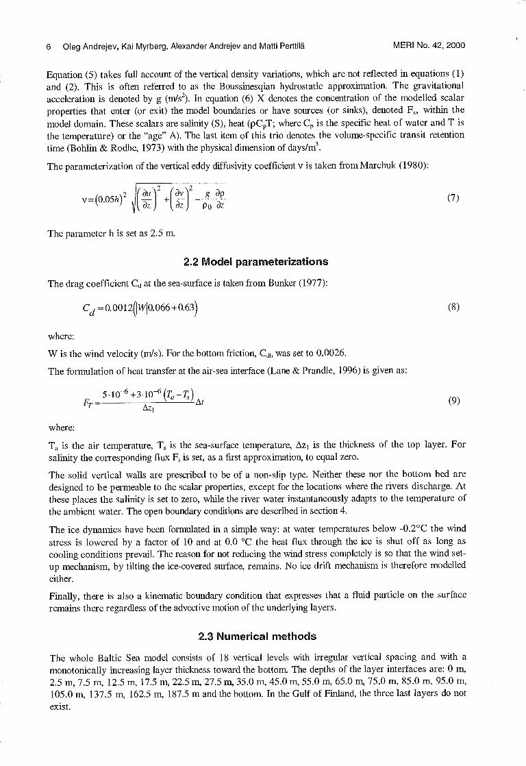
BaltBath tools contains a data editor module to manually modify data arrays. A right mouse click in a map will call up a "Data Editor" dialog (Fig. 11). The 100 data array nodes nearest to cursor position will be loaded into a data array. The Colour Map grid, located in the lower part of the dialog, represents loaded data with the current chart palette settings.

A left mouse click over the Colour Map will select the corresponding cell in the data array.

To modify a data array node value, the cell is selected, the value is edited and Enter is pressed. The Colour Map grid reflects the changes.

To confirm the changes and return to working with the array data, "OK" is pressed; otherwise "Cancel" may be used. The data file is saved by selecting the "File - Save" or "File-Export" main menu items.

Warning! The basic data arrays IOWBALT1, IOWBALT2 are not protected from changes.

3.7 How to save bathymetry data

The BaltBath tool provides three methods for saving a prepared data array. The user can save it in fast binary format (a sdf file) by picking the "File - Save" main menu item. BaltBath supports two data export formats: a comma- separated ASCII-file (File - Export - ASCII) and the DAS data format (File - Export - DAS).

The user can also transfer prepared data to MS Excel, if this software is installed on the computer in use. It is not necessary to load MS Excel beforehand since, BaltBath, using OLE-technology, does this itself.

Hydrodynamic and chemical modelling of the Baltic Sea - a three-dimensional modelling approach 15

Data Editor

Data Edåor:g:

1302 1303 4 1305 1346 307 1308 1'

: 361 :75.00 85.00 ; 90.00 105.00 110.00 115.00 120.00 120.00 120.00 '.125.00

362 60.00 85.00 , 90.00 110.00 120.00 ' 130.00 125.00 125.00 120.00 115.00

363 25.00 80.00 , 95.00 105.00 105.00 125.00 130.00 125.00 120.00 ' 115.00

36# 30.00 50.00 70.00 95.00 95.00 ' 110.00 120.00 125.00 120.00 ' 110.00

5.00 45.00 60.00 70.00 95.00 110.00 120.00 120.00 120.00 125.00

366 0.00 5.00 45.00 ! 50.00 ' 90.00 105.00 ' 110.00 115.00 120.00 ' 125.00

367 0.00 0.00 0.00 20.00 45.00 75.00 105.00 110.00 115.00 120.00 _......_ ~ 0.00 0.00 0.00 0.00 5.00 60.00 80.00 105.00 110.00 110.00

369 10.00 0.00 0.00 0.00 6.00 0.00 50.00 100.00 100.00 105.00

370 0.00 2.00 0.00 0.00 6.00 0.00 5.00 70.00 65.00 ', 80.00

Color Map :

11111111111EEEERIMIN ■■s■■■ 1111111111111111111EEME

MI MI 1212 3,VM,111 NI WINNE MI

■■■ ■

Fig. 11. Data Editor dialog.

3.8 Graphical Means

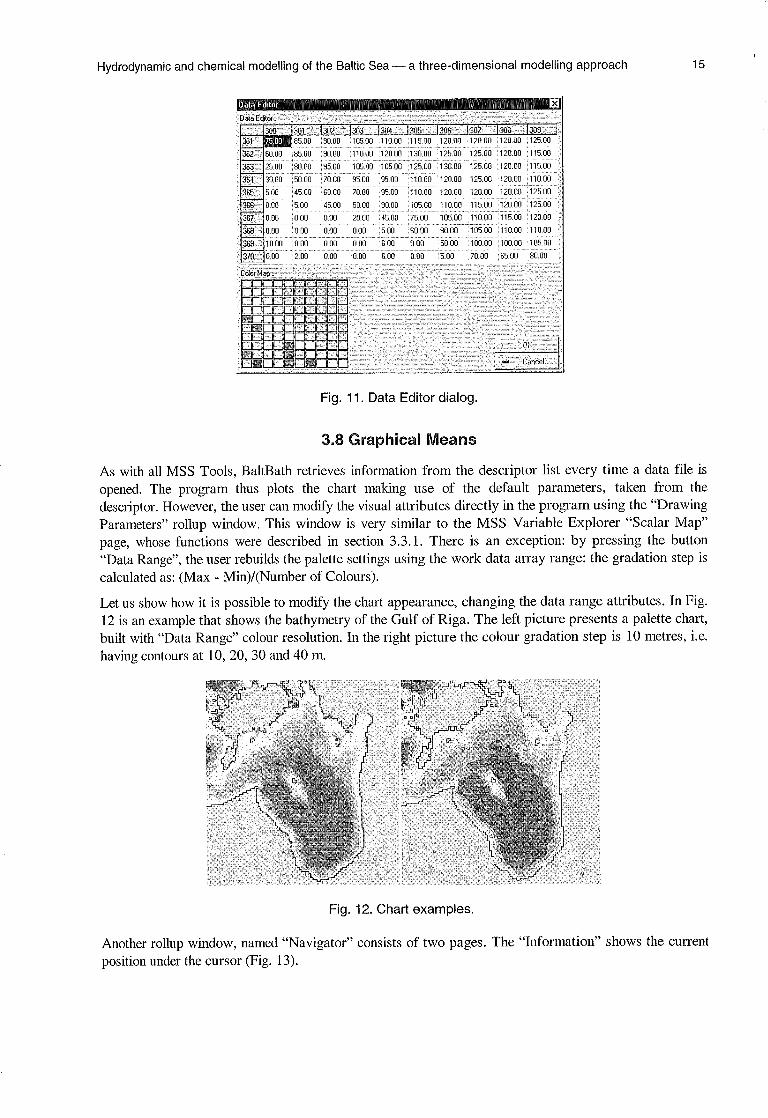
As with all MSS Tools, BaltBath retrieves information from the descriptor list every time a data file is opened. The program thus plots the chart making use of the default parameters, taken from the descriptor. However, the user can modify the visual attributes directly in the program using the "Drawing Parameters" rollup window. This window is very similar to the MSS Variable Explorer "Scalar Map" page, whose functions were described in section 3.3.1. There is an exception: by pressing the button "Data Range", the user rebuilds the palette settings using the work data array range: the gradation step is calculated as: (Max - Min)/(Number of Colours).

Let us show how it is possible to modify the chart appearance, changing the data range attributes. In Fig. 12 is an example that shows the bathymetry of the Gulf of Riga. The left picture presents a palette chart, built with "Data Range" colour resolution. In the right picture the colour gradation step is 10 metres, i.e. having contours at 10, 20, 30 and 40 m.

Fig. 12. Chart examples.

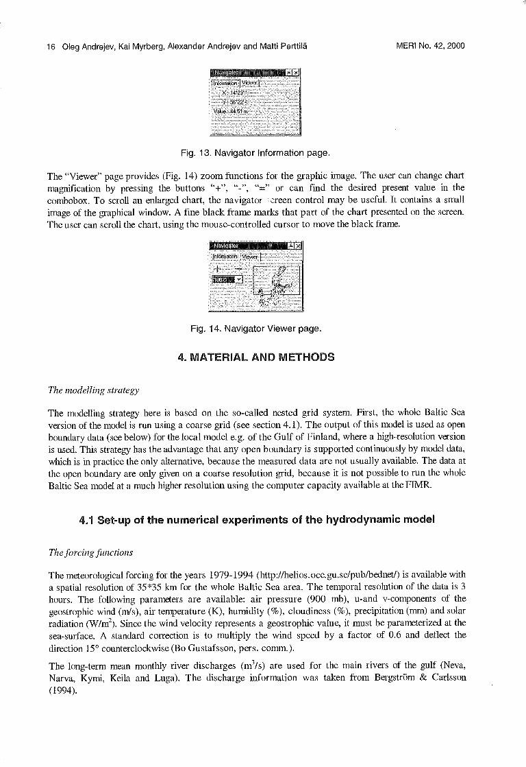
Another rollup window, named "Navigator" consists of two pages. The "Information" shows the current position under the cursor (Fig. 13).

Informahon ~ View

x:14'23'° Y : 58°22'

lue a.44.51 m

Information


Navigator"

Fig. 13. Navigator Information page.

The "Viewer" page provides (Fig. 14) zoom functions for the graphic image. The user can change chart magnification by pressing the buttons "+", "-", "=" or can find the desired present value in the combobox. To scroll an enlarged chart, the navigator creen control may be useful. It contains a small image of the graphical window. A fine black frame marks that part of the chart presented on the screen. The user can scroll the chart, using the mouse-controlled cursor to move the black frame.

Navigator

Fig. 14. Navigator Viewer page.

4. MATERIAL AND METHODS

The modelling strategy

The modelling strategy here is based on the so-called nested grid system. First, the whole Baltic Sea version of the model is run using a coarse grid (see section 4.1). The output of this model is used as open boundary data (see below) for the local model e.g. of the Gulf of Finland, where a high-resolution version is used. This strategy has the advantage that any open boundary is supported continuously by model data, which is in practice the only alternative, because the measured data are not usually available. The data at the open boundary are only given on a coarse resolution grid, because it is not possible to run the whole Baltic Sea model at a much higher resolution using the computer capacity available at the FIMR.

4.1 Set-up of the numerical experiments of the hydrodynamic model

The forcing functions

The meteorological forcing for the years 1979-1994 (http://helios.oce.gu.se/pub/bednet/) is available with a spatial resolution of 35*35 km for the whole Baltic Sea area. The temporal resolution of the data is 3 hours. The following parameters are available: air pressure (900 mb), u-and v-components of the geostrophic wind (m/s), air temperature (K), humidity (%), cloudiness (%), precipitation (mm) and solar radiation (W/m2). Since the wind velocity represents a geostrophic value, it must be parameterized at the sea-surface. A standard correction is to multiply the wind speed by a factor of 0.6 and deflect the direction 15° counterclockwise (Bo Gustafsson, pers. comm.).

The long-term mean monthly river discharges (m3/s) are used for the main rivers of the gulf (Neva, Narva, Kymi, Keila and Luga). The discharge information was taken from Bergström & Carlsson (1994).


The simulation period

The simulation period of the hydrodynamic model experiment was August 1, 1987-July 31, 1988.

The modelled area and resolution

The open boundary of the Baltic Sea model domain is placed in the Kattegat along latitude 57°35'N. The Gulf of Finland model domain has two open boundaries, the western one corresponding to longitude 22°32'E and the southern one corresponding to latitude 59°05'N. Both models have the same vertical resolution. The whole Baltic Sea model consists of 18 vertical layers, while the Gulf of Finland model has 15 layers. The horizontal resolution of the Baltic Sea model is 5*5 nautical miles and that of the Gulf of Finland 1*1 nautical miles.

The initial conditions

The initial temperature and salinity fields both for the whole Baltic Sea and for the Gulf of Finland model versions were constructed using the Data Assimilation System (DAS) developed in the Department of Systems Ecology in the University of Stockholm (Sokolov & al., 1997). The DAS is coupled with the Baltic Environmental Database (BED) (Wulff & Rahm, 1991) and with the 3D hydrodynamic model (Andrejev & Sokolov, 1992). The latter gives additional benefits and allows one to use the DAS

graphical possibilities for presentation of the model results. To construct the initial fields for August 1987 (the first month of the numerical experiment), temperature and salinity data from BED for all Augusts from 1980 to 1992 were used. The experiment started from the quiescent state.

The open boundary conditions

A combination of the Sommerfeld radiation condition (Sommerfeld, 1949; Orlanski, 1976) and relaxation to the boundary values is used at the open boundaries. The radiation condition is provided by

aq dq +c 2 =0

where: q is temperature, salinity or surface elevation, t is time, n is a normal to the open boundary and c is the propagation (phase) speed normal to the boundary. The finite-difference form of eq (14) for the western boundary is obtained using forward-in-time, upstream differencing (Greatbatch & Otterson, 1991)

n+1n At n n _ gb — qb — c Ax

(it — gb+1) (15)

where: At is a time step, Ax is a space step, the superscript n denotes time level and the subscript b is an abbreviation for the word "boundary". A variable with the subscript b + 1 refers to a grid point which is one space step in the domain away from the boundary and q6 denotes a value calculated with the coarse resolution Baltic Sea model. The phase speed can be determined as

A(qn qbn

- b+1 +1

1

c=

C=C 1f0< C < Cm~

c =Cmax lf C >Cmax

(14)

At(qb+1 qb+2 ra-1 _ n-1

(16)


c=—y Ö ifc <-0

Where Cm = 767t and y is the relaxation parameter, and 0 < y < 1.

To realise the radiation condition, the spatial derivative of the depth normal to the boundary must be equal to zero:

dn

The models are constructed on the C-grid, and therefore the velocities in the Coriolis-terms are calculated as the average of the velocities at the four nearest grid points, the v-components for the u—momentum equation and vice versa. At open boundaries two of these points are outside the model domain. To avoid numerical problems in this case, we transfer the corresponding velocity components from the coarse resolution model of the Baltic Sea.

Relaxation to the open boundary values calculated by the coarse resolution model could be also realised by the specific form of the horizontal diffusive terms (Mutzke, 1998) in which

n+1 (Ron — Rb

= n a — (kb', — Rb+i

(17) µH ~R b µH (Ax )2

where: R is the temperature, salinity or velocity component, Rid is its prescribed value transferred from the coarse resolution model or observed, µ H is the horizontal diffusion coefficient, a is the relaxation coefficient, whose range (O'Brien, 1986) is

0<a<8

2

A t

However, this relaxation approach is not used here.

The calculation of the retention time of water

An age for the water is described by the advection-diffusion equation (Deifies & al. 1999), that has the same form as that used for heat or salinity transport, but with the physical dimension of age per unit volume. The added dynamics is the source term which adds the "age" to water parcels which are in the modelled area. The specific age for the water at an open boundary is set to zero, and this also applies to river discharge water. As well as the dynamics included in the advection-diffusion equation, the water age is also controlled by the vertical convection parametrization (see section 2.4). This form of retention time analysis has become an accepted procedure (Mattson, 1996; Gustafsson, 1997).

The calculation of the mean circulation and stability

Witting (1912) and Palmen (1930) defined the stability, or persistency, of the current R as the ratio between its vector mean speed and scalar mean speed:

aH

R=

i Lttn +J1,l'n 100% (18)

2 2 +v,t


where: the horizontal vector velocity V is defined as:

V=ui +vj

The velocity components are saved at every time step (in our simulations at 30 minute intervals); n denotes the total number of time steps (velocity components at each point) used in the averaging procedure. In a one-year simulation n is thus about 17 520 (2*24*365).

As a result of the above procedure, the vector mean speed, scalar mean speed and the stability can be determined at each grid point at each time step, and averaged values of these parameters are available over any time period.

4.2 Set-up of numerical experiments of the chemical model

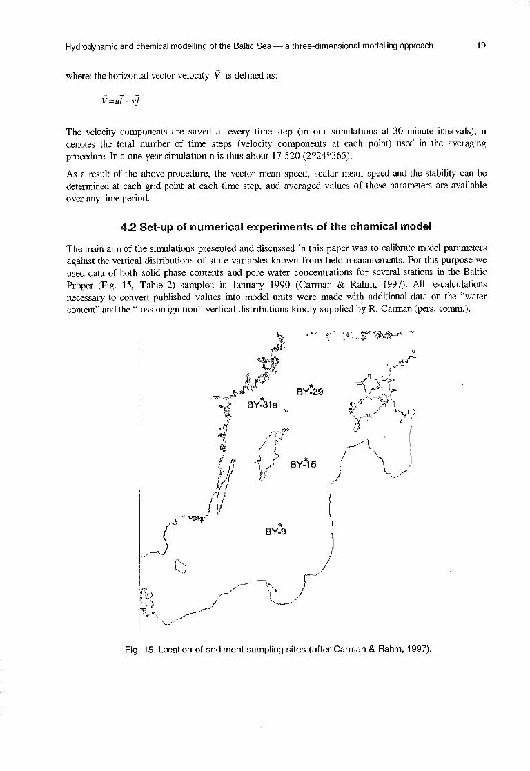
The main aim of the simulations presented and discussed in this paper was to calibrate model parameters against the vertical distributions of state variables known from field measurements. For this purpose we used data of both solid phase contents and pore water concentrations for several stations in the Baltic Proper (Fig. 15, Table 2) sampled in January 1990 (Carman & Rahm, 1997). All re-calculations necessary to convert published values into model units were made with additional data on the "water content" and the "loss on ignition" vertical distributions kindly supplied by R. Carman (pers. comm.).

Fig. 15. Location of sediment sampling sites (after Carman & Rahm, 1997).


Table 2. Near-bottom (nbw') and pore water (pw2) concentrations of nutrients, oxygen and hydrogen sulphide (pM), compiled from Tables 1 and 2 in Carman & Rahm (1997).

Station Depth (m) N1 a-N nbw pw

NO3-N3 nbw pw nbw

PO4-P pw

02/H2S4 nbw pw

BY 9 91 0.5 67.7 10.95 - 2.34 12.1 109.3/- 14.0 BY 15 248 14.7 424.5 - - 8.34 18.4 -/88.8 223.3 BY 29 181 0.31 22.5 7.87 - 3.33 4.4 -/6.0 9.0 BY 31s 125 0.2 30.0 9.33 - 2.78 1.2 81.2/- 0.0

'Nutrients samples were collected at about 3-5 m above the bottom, oxygen/hydrogen sulphide were sampled about 0.5 m above the sediment surface. 2Pore water concentrations from the topmost centimetre of sediments. 3No data on nitrate concentration in the pore water were published. `'For pore water, only hydrogen sulphide concentrations were published.

Since these samples were taken during the long stagnation period that started in the Baltic Sea in the late 70's, the bottom water at the two deepest stations BY 15 and BY 29 were anoxic, while hydrogen sulphide was already present in the uppermost centimetre of sediments at site BY 9 with oxic bottom water. The only exception was that at BY31s hydrogen sulphide was not found at all within the upper three cm of the sediment sample. At this site both the grain size was coarser than that of the other sites and the porosity was the lowest. However, no signs of macrofauna were found either at this site or at the others.

Ammonium and phosphate production rates were calculated from the data presented by Carman & Rahm (1997), using a multi-G approach (Berner, 1980; Westrich & Berner, 1984) as modified by Carignan & Lean (1991) to account for the variable porosity and compaction within the upper layers of sediments. The specific nitrogen and phosphorus mineralization rates were estimated from the field data.

Initial estimates for the other parameters were derived from the available literature.

The numerical experiments were performed for the upper 10 cm of sediments with a 1-mm space step and 1-day time step.

5. THE MODEL SIMULATIONS

5.1. The results of the hydrodynamic modelling

The preliminary results of the hydrodynamic modelling studies are presented primarily for the Gulf of Finland. The following main aspects have been studied using the model: the mean circulation of the gulf and its stability, the retention time of the water, the water exchange with the Baltic Sea Proper, the horizontal and vertical structure of salinity, sea-level variations and upwellings, and related sea temperature changes. The basic physical processes are also discussed in connection with the simulations.

5.1.1 The hydrodynamics of the Gulf of Finland

The Gulf of Finland is an interesting sea-area in the Baltic Sea because of its complicated hydrographic nature. The western end of the gulf is a direct continuation of the Baltic Sea Proper, whereas the eastern end of the gulf receives the largest single fresh water input to the whole Baltic Sea, namely the River Neva, with a mean input of about 2700 m3/s. This leads to a continuous east-west salinity gradient in the gulf. The stratification conditions are very variable in space and time for the above-mentioned reasons and because of the large seasonal variations in incoming solar radiation. The density-driven circulation is an important factor in modifying currents in the gulf, in addition to the wind forcing and the forcing


introduced by the surface slope. The hydrographic features are also strongly modified by the variable and complex bottom topography. A line between the Hanko peninsula and the island of Osmussaar is often treated as the western boundary of the gulf. The hydrodynamics of the gulf is described in detail by Alenius & al. (1998).

5.1.2 The vertical and horizontal structure of salinity

As stated above, the opposite effects of the saline water inflow from the Baltic Sea Proper and the inflow of fresher waters from the rivers leads to a continuous east-west salinity gradient in the gulf. The horizontal variation of salinity in an east-west direction is 6-7 per mill/400 km. The salinity increases from east to west and from north to south. The surface salinity varies from 5-7 per mill in the western gulf to about 0-3 per mill in the east. Between Helsinki and Tallinn, the surface salinity is typically between 4.5-5.5 per mill. The bottom salinity in the western gulf can typically reach values of 8 per mill or even more, especially after the saline water pulse into the Baltic Sea in 1993. In the western gulf, a permanent halocline exists throughout the year between depths of some 60-80 m. The existence of the halocline prevents vertical mixing of the water body down to the bottom. The variability of bottom salinity in the western gulf and related changes in the halocline are connected with an irregular intrusion of Baltic Sea deep water, which penetrates into the gulf along the slope of the bottom, the latter lacking any thresholds. The intrusion of salinity in the near-bottom layer is most probably related to the joint effect of baroclinicity and bottom relief JEBAR (Sarkisjan & al. 1975; Mälkki & Tamsalu, 1985). Often frontal areas are observed in the south-western gulf separating the Baltic Sea waters from the less saline gulf water (see e.g. Mälkki & Talpsepp, 1988; Kononen & al. 1996; Pavelson & al. 1996; Laanemets & al. 1997). The surface layer salinity decreases from winter to mid-summer while at the same time the salinity of the deep layers increases. Between March and July, the surface layer salinity can decrease e.g. from 6 to 4.5 per mill while the salinity increases at a depth of 60 metres from 7 to 9 per mill. Towards the east, the difference between surface and bottom salinity decreases. The surface layer salinity variations are easily understood as being related to the melting of the ice cover and the increased spring-time Neva runoff. The surface layer outflow seems to generate an inflow into the gulf in the deeper layers (Haapala & Alenius, 1994).

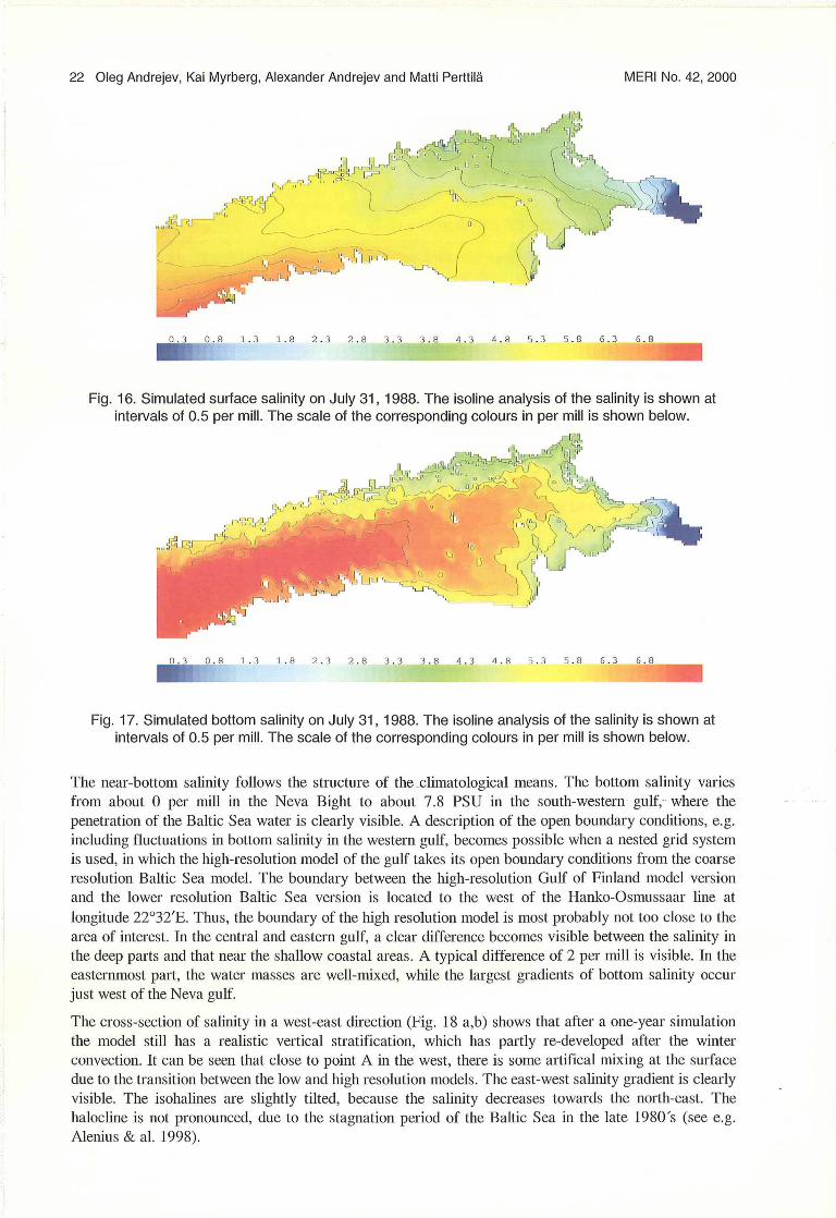
The simulated fields of surface (Fig. 16) and bottom salinity (Fig. 17) are given for July 31, 1988 after a simulation of one year. The model reproduces the horizontal large-scale structure of surface salinity well when compared with climatology (Jurva, 1951) and with verified model results (Myrberg, 1997). The surface salinity varies from about 0 per mill in the Neva Bight to about 6.8 per mill at the mouth of the gulf. One of the most interesting results of the simulation is that the isolines of salinity are not purely north-south—oriented (i.e. east-west gradients). The water mass in the northern gulf is fresher than the water along the southern coast. This due to the fact that the fresh water from the Neva and Kymi Rivers flow westwards along the Finnish coast. This feature was not described accurately by Myrberg (1997) probably mainly because of the lower horizontal resolution of the model (4.5*4.5 km) compared with tha used at present (1*1 nautical mile). The surface salinity pattern indirectly supports the assumption of a cyclonic circulation in the gulf: the fresh surface water flows out from the gulf along the Finnish coast, whereas the inflow of more saline water takes place along the Estonian coast (see section 5.1.5).

~.,̂ ~f✓~ .-, 4

, r_~ v =t,, ~ 4, .

41

I~S

~

II I

0.3 0.8 1.3 1.8 2.3 2.8 3.3 3.8 4.3 4.8 5.3 5.8 6.3 6.8


08 1.3 1.8 2.3 2.8 3.3 3.8 4 3 4.8 5.3 5.8 6.3 6.8

11111P1.3 11

Fig. 16. Simulated surface salinity on July 31, 1988. The isoline analysis of the salinity is shown at intervals of 0.5 per mill. The scale of the corresponding colours in per mill is shown below.

Fig. 17. Simulated bottom salinity on July 31, 1988. The isoline analysis of the salinity is shown at intervals of 0.5 per mill. The scale of the corresponding colours in per mill is shown below.

The near-bottom salinity follows the structure of the climatological means. The bottom salinity varies from about 0 per mill in the Neva Bight to about- 7.8 PSU in the south-western gulf, where the penetration of the Baltic Sea water is clearly visible. A description of the open boundary conditions, e.g. including fluctuations in bottom salinity in the western gulf, becomes possible when a nested grid system is used, in which the high-resolution model of the gulf takes its open boundary conditions from the coarse resolution Baltic Sea model. The boundary between the high-resolution Gulf of Finland model version and the lower resolution Baltic Sea version is located to the west of the Hanko-Osmussaar line at longitude 22°32'E. Thus, the boundary of the high resolution model is most probably not too close to the area of interest. In the central and eastern gulf, a clear difference becomes visible between the salinity in the deep parts and that near the shallow coastal areas. A typical difference of 2 per mill is visible. In the easternmost part, the water masses are well-mixed, while the largest gradients of bottom salinity occur just west of the Neva gulf.

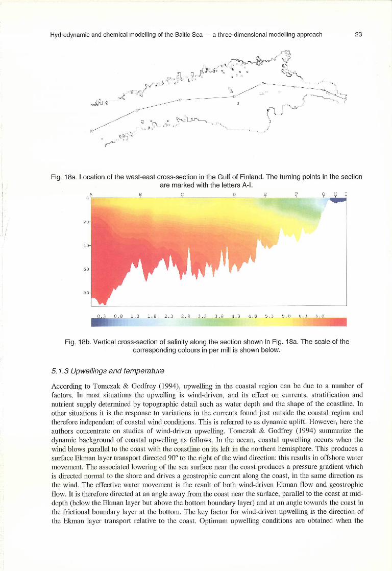
The cross-section of salinity in a west-east direction (Fig. 18 a,b) shows that after a one-year simulation the model still has a realistic vertical stratification, which has partly re-developed after the winter convection. It can be seen that close to point A in the west, there is some artifical mixing at the surface due to the transition between the low and high resolution models. The east-west salinity gradient is clearly visible. The isohalines are slightly tilted, because the salinity decreases towards the north-east. The halocline is not pronounced, due to the stagnation period of the Baltic Sea in the late 1980's (see e.g. Alenius & al. 1998).

E H I

4.8 5.3 3.8 6.3 6.8


Fig. 18a. Location of the west-east cross-section in the Gulf of Finland. The turning points in the section are marked with the letters A-I.

B C D

20

40

60

80

0.3 0.8 1.3 1.8 2.3 2.8 3.3 3.8 4.3

Fig. 18b. Vertical cross-section of salinity along the section shown in Fig. 18a. The scale of the corresponding colours in per mill is shown below.

5.1.3 Upwellings and temperature

According to Tomczak & Godfrey (1994), upwelling in the coastal region can be due to a number of factors. In most situations the upwelling is wind-driven, and its effect on currents, stratification and nutrient supply determined by topographic detail such as water depth and the shape of the coastline. In other situations it is the response to variations in the currents found just outside the coastal region and therefore independent of coastal wind conditions. This is referred to as dynamic uplift. However, here the authors concentrate on studies of wind-driven upwelling. Tomczak & Godfrey (1994) summarize the dynamic background of coastal upwelling as follows. In the ocean, coastal upwelling occurs when the wind blows parallel to the coast with the coastline on its left in the northern hemisphere. This produces a surface Ekman layer transport directed 90° to the right of the wind direction: this results in offshore water movement. The associated lowering of the sea surface near the coast produces a pressure gradient which is directed normal to the shore and drives a geostrophic current along the coast, in the same direction as the wind. The effective water movement is the result of both wind-driven Ekman flow and geostrophic flow. It is therefore directed at an angle away from the coast near the surface, parallel to the coast at mid-depth (below the Ekman layer but above the bottom boundary layer) and at an angle towards the coast in the frictional boundary layer at the bottom. The key factor for wind-driven upwelling is the direction of the Ekman layer transport relative to the coast. Optimum upwelling conditions are obtained when the

16.0 1II.0 12.0

-rF4jr.'

©.0


Ekman transport divergence is maximized, which occurs when the Ekman transport is directed offshore and normal to the coastline.

The upwelling in the Gulf of Finland has been studied by several authors, and its role is found to be significant. It brings nutrient-rich water from deeper layers to the surface, mixes water masses and generates frontal areas. During upwelling, the surface temperature can drop by about 10 degrees in a few days. The biological consequences of upwelling can be significant (see Hela, 1976; Kononen & Niemi, 1986; Haapala, 1994). On the Finnish coast it is associated with a south-westerly wind, which has to last for about 2-3 days at least to cause upwelling. Upwelling becomes clearly visible in summer when strongly stratified conditions exist and the effect of wind stress is distributed through a shallow water layer. A wind impulse of about 4000-9000 kgni's' is needed to cause upwelling (Haapala, 1994). Vertical velocities can reach values of 4-10*10-3cros' (Hela, 1976).

The model was used to test its ability to produce upwelling. The model was run with typical stratification conditions for August with a surface temperature of about 15-17 degrees. Two test simulations were carried out. In both cases the water level and currents were set to zero at the beginning of the simulations. In the first case, the model was run for five days with a constant wind forcing of 10 m/s from the south-west and with a constant air temperature of 17 degrees. The south-westerly wind was used in order to maximize the Ekman transport divergence. As was to be expected, a clear upwelling took place along the northern coast of the gulf, with a drastical drop of surface temperatures there (Fig. 19). Such events have been observed in reality e.g. in Tvärminne (see e.g. Hela, 1976, Haapala, 1994). In the simulated case, the horizontal temperature gradient at the surface is pronounced, with maximum values of temperature near 20 degrees on the eastern gulf while the lowest temperatures on the Finnish coast are about 9 degrees. If a cross-section in the area of the highest sea-surface temperature gradient is studied (Fig. 20 a,b), it is seen that a pool of cold bottom water has been brought up to the surface on the northern coast, whereas on the southern coast warm surface water is observed. The temperature difference at the surface is about 10 degrees. The cross-section also shows the clear tilting of the thermocline. On the southern coast the well-mixed layer is rather deep, whereas on the northern coast the thermocline is near the surface.

Fig. 19. Surface (0-2.5 m) temperature field after a simulation of 5 days with a 10 m/s wind from the

south-west. The scale of the corresponding colours in °C is shown below.

Hydrodynamic and chemical modelling of the Baltic Sea a three-dimensional modelling approach 25

Fig. 20a. Location of the north-south cross-section in the Gulf of Finland. The beginning and end points of the section are marked A and B.

B

0-

8.0 10.0

12.0 14.0

11.0 16.0

Fig. 20b. Vertical cross-section of temperature along the section shown in Fig. 20a. The cross-section corresponds to Fig. 19. The scale of the corresponding colours in °C is shown below.

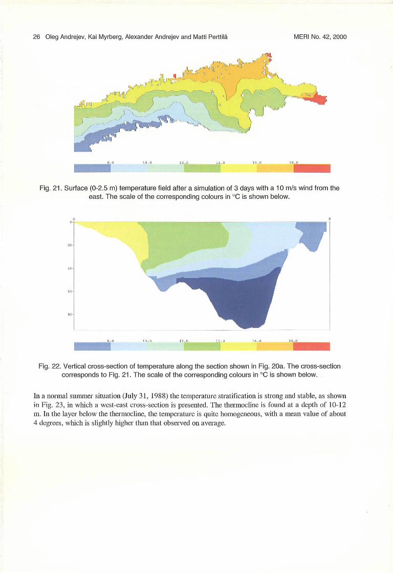
In the second experiment the only differences compared with the first simulation are that the wind blows from the east with speed of 10 m/s and that the simulation period is only 3 days. An easterly wind was used in order to maximize the Ekman transport divergence. The opposite situation compared with the first experiment is observed (Fig. 21). On the Estonian coast the surface temperature dropped to about .6 degrees, while the highest temperatures are still near 20 degrees in the east. A cross-section across the highest sea-surface temperature gradient shows (Fig. 22) that a pool of cold water is located on the Estonian coast, while the warmest water masses are found on the Finnish coast. The temperature difference between the coldest and warmest water masses is just the same as in the first case. Now, the well-mixed layer in the north is rather deep, while on the southern coast the thermocline is near the surface. The thermocline is again tilted between the northern and the southern coasts, but the tilting is opposite to that of the first experiment.


'1'11J Nkr,`„~'-f'~~

Ja n

~ : `~~/

~n ,.

';r`~~~ tii

_rgr?J

S ~~~~/~

10.0 12.0 16.0 16.0

Fig. 21. Surface (0-2.5 m) temperature field after a simulation of 3 days with a 10 m/s wind from the east. The scale of the corresponding colours in °C is shown below.

6.0 10. 0

12.0

14 .0 16.0 16.0

Fig. 22. Vertical cross-section of temperature along the section shown in Fig. 20a. The cross-section corresponds to Fig. 21. The scale of the corresponding colours in °C is shown below.

In a normal summer situation (July 31, 1988) the temperature stratification is strong and stable, as shown in Fig. 23, in which a west-east cross-section is presented. The thermocline is found at a depth of 10-12 m. In the layer below the thermocline, the temperature is quite homogeneous, with a mean value of about 4 degrees, which is slightly higher than that observed on average.

Hydrodynamic and chemical modelling of the Baltic Sea - a three-dimensional modelling approach 27

0.6 1.0 3.0 4.2 5.4 6.6 7.8 9.0 10.2 11.4 12.6 13.8 15.0 16.2 17.4 18.6 19.8

~! Mir

Fig. 23. Surface (0-2.5 m) temperature field on July 31, 1988. The scale of the corresponding colours in °C is shown below. Location of the cross-section is shown in Fig. 18a.

5.1.4 Sea-level variations

Sea-level variations are forced by three main factors: variations in the wind direction and speed, air pressure fluctuations and changes in the density of the sea water (Lisitzin, 1958; 1974).

Sea-level measurements have been made in Finland for more than 100 years, since 1887, Hanko being the first station. These measurements are worth mentioning as important material for climate change studies, because they have been made relative to bed rock and can be considered as being very reliable. The only relevant disturbing effect is the land uplift, which in the gulf is 2.3 mina-1 (Vermeer & al. 1988). Several studies have been devoted to the sea-level problem (see e.g. Witting, 1911; Hela, 1944; Lisitzin, 1944, 1959a, 1966; Stenij & Hela, 1947). High water levels have been a real nuisance for the population of St. Petersburg. Since 1703 the city has been flooded more than 280 times. The highest water level measured was 421 cm in 1824. A significant part of the sea-level oscillations is caused by free-standing waves, seiches, that are manifested when an external force ceases. The period of an uninodal oscillation of the Baltic Proper-Gulf of Finland system is 26.2 h on average (Lisitzin, 1959b). Tidal motions in the gulf, as in the whole Baltic Sea, are negligible, their mean amplitudes being only some millimetres or centimetres (Listizin, 1944). This effect is therefore not taken into account in the model equations.

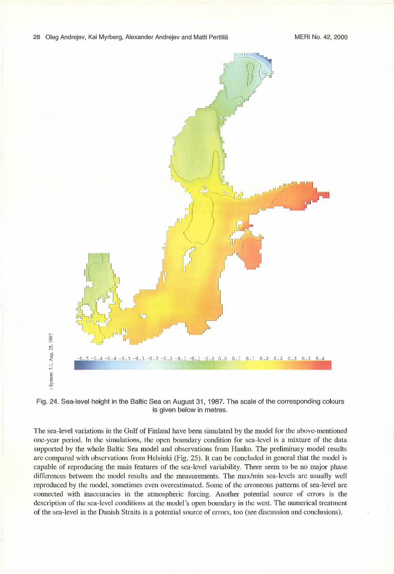
The sea-level variations in the Baltic Sea using the coarse grid are shown in Fig. 24. The figure represents the sea-level on August 31, 1987. The sea-level distribution is logical for a situation in which a cyclone is located over the Baltic Sea. The mean sea-level is thus about zero in the central Baltic, while maximal sea-levels of +0.5 m are recorded in the eastern extremity of the sea, i.e. in the Gulf of Finland; this can be explained by the fact that the mean wind is from the south-west and thus the mean Ekman transport is directed into the Gulf of Finland. In general the eastern side of the Baltic- Sea is characterized by positive sea-levels, due to winds from the south-west or west. In the Gulf of Bothnia- area, the wind is blowing from the north and thus the minimum sea-level is observed there with values of -0.5 m. It also turns out that there is a slight sea-level difference between the Baltic Sea and the North Sea, which plays a important role in the water exchange between these seas.


-0.5 -0.4 -0.4 -0.3 -0.3 -0.2 -0.2 -0.1 -0.1 -0.0 0.0 0.1 0.1 0.2 0.2 0.3 0.3 0.4

Syst

em 3

.1, A

ug,

25,

199

7

Fig. 24. Sea-level height in the Baltic Sea on August 31, 1987. The scale of the corresponding colours is given below in metres.

The sea-level variations in the Gulf of Finland have been simulated by the model for the above-mentioned one-year period. In the simulations, the open boundary condition for sea-level is a mixture of the data supported by the whole Baltic Sea model and observations from Hanko. The preliminary model results are compared with observations from Helsinki (Fig. 25). It can be concluded in general that the model is capable of reproducing the main features of the sea-level variability. There seem to be no major phase differences between the model results and the measurements. The max/min sea-levels are usually well reproduced by the model, sometimes even overestimated. Some of the erroneous patterns of sea-level are connected with inaccuracies in the atmospheric forcing. Another potential source of errors is the description of the sea-level conditions at the model's open boundary in the west. The numerical treatment of the sea-level in the Danish Straits is a potential source of errors, too (see discussion and conclusions).

40 —

Leve

l, cm

20

-20 —

-40 —

Observations of

Model results

~I

Hydrodynamic and chem

80 —

60 —

cal modelling of the Baltic Sea a three-dimensional modelling approach 29

Ö 1.11

Time, hours

Fig. 25. Sea-level observations from Helsinki (continuous line) and the corresponding model results (dashed line) for the period August 1-November 31, 1987. The sea-level height is given in centimetres.

5.1.5 The mean circulation

The main forcing factor for currents in the Gulf of Finland, as in the whole Baltic Sea, is the wind stress. Density-driven currents also play an important role in the overall circulation due to the pronounced horizontal density (buoyancy) gradients caused by the variations in salinity and temperature. The sea-surface slope that results from the permanent water supply to the eastern part of the gulf also contributes appreciably to the existing circulation pattern. The gulf is large enough to see the effects of the earth's rotation, too (Witting, 1912; Palm6n, 1930; Hela, 1946).

The importance of the mean circulation is often discussed. However, there are many open questions to be answered. There is no clear vision of how much the circulation varies interannually and/or seasonally and what the mean circulation pattern looks like in detail, even though there is physical reasoning for the general existence of a cyclonic circulation. It is also not fully known what the average current velocity and the stability of the current is. It would be interesting to discover the value of the water volume which is exchanged between the gulf and the Baltic Sea Proper, because only a few numbers for it are available (Witting, 1912; Lehmann & Hinrichsen, 2000). Closely connected with the water exchange is the problem concerning estimation of the retention time of the water; i.e. how. "old" the water in the Gulf of Finland is.

The knowledge of the mean circulation, even if the latter is a statistical phenomena and not a true physical circulation as Palma. (1930) stated, can be used for many purposes. The mean circulation field can be used to discuss e.g. the average conditions for the dispersion of pollutants or what is the probable horizontal distribution of nutrients. Also many practical activities, such as shipping and coastal building (sea ports, terminals etc.), need information concerning the mean current conditions and their variability. Knowledge of the retention time of water masses gives us the possibility of estimating the time-scale on which the pollutants gradually dilute in the Baltic Sea waters and sink to the bottom. Estimates of the water exchange between the gulf and the Baltic Sea Proper enable us to study the water balance of the gulf in more detail. Estimates of the water exchange and its variability can be used e.g. in box models, in which estimates of the fluxes between the boxes are needed.


The simulated mean surface current field (0-2.5 m) for the period August 1, 1987-July 31, 1988 is given in Fig. 26. The field, consisting of nearly 10 000 calculation points, is characterised by an eddy-like structure and many frontal areas are visible. The horizontal resolution of one nautical mile should be enough to describe the internal Rossby-radius of deformation scale, which is about 2-4 kilometres in the gulf (Alenius & al. 2000). The overall structure of the field contains the basis of a cyclonic circulation, but in a very complex form with several separate cells. There is a clear tendency for water to come into the gulf along the Estonian coast and to move far eastwards. In the western gulf the inflow-outflow pattern is pronounced, forming a clearly cyclonic circulation system. Another clear feature is the voluminous outflow from the River Neva. The outflow from the gulf seems to take place in the northern part of the central area of the gulf with a meandering structure. The shallow northern coastal waters seem to play no key role in the overall circulation. There is clear tendency for mean surface currents to be directed northwards in the central gulf (longitude 25°30'E), connected most probably with the frontal structure of salinity and/or steering by the bottom topography. The simulated mean vector average surface current velocity in the gulf is definitely higher than suggested by Witting (1912) and Palm6n (1930), who studied a five-year period.

Gulf of Finland western part

Gulf of Finland eastern part

Fig. 26. Mean surface circulation (0-2.5 m) in the Gulf of Finland for the period August 1, 1987-July 31, 1988. The scale of the current (cm/s) is given below.

A 0--

20

~


5.1.6 Retention time, stability and water exchange

The mean u-component of the vector velocity for the period August 1, 1987-July 31, 1988 at the Hanko-Osmussaar cross-section is given in Fig. 27. It becomes clearly visible that on the Estonian coast there is a tendency for inflow of water with a mean velocity of c. 8 cm/s. There is weak inflow over the whole southern gulf, with a maximum also in the middle of the gulf in the near-bottom layer. A mean inflow velocity of 5 cm/s is observed. On the Finnish side, there is intense outflow, except in the very shallow coastal region. The maximum outflow velocity is about 8 cm/s with values of 5 cm/s being typical, which is in accordance with the estimates of Sarkkula (1991) based on current measurements in the gulf. The mean inflow structure presented here again strongly supports the idea of a cyclonic circulation.

-9.0 9.(I

9.0

1111 Fig. 27. Mean cross-section of the u-component of velocity for the period August 1, 1987-July 31, 1988 at the entrance of the Gulf (Hanko-Osmussaar). The scale of the corresponding colours is given below

in cm/s. Positive numbers indicate flow into the gulf and negative numbers indicate outflow from the gulf.

According to the model the difference between inflow and outflow is about 108 km3/s, meaning that the inflow is that much smaller than the outflow. The difference can be explained as being due to the river runoffs into the gulf, which total approximately 115 km3/s. It should be stressed that the difference between precipitation and evaporation is not taken into account in the present model runs, but in the gulf this difference is usually small (Myrberg, 1998). Lehmann & Hinrichsen (2000) have calculated the differences between the in-and outflows e.g. for 1986 and 1988, finding values of 142 km3/s and 148 km3/s, which are larger than ours. Witting (1912) got a long-term mean of 120 km3/s.

The horizontal distribution of the retention time for the corresponding period is in accordance with the previous analyses (Fig. 28). The shortest retention time is observed on the Estonian coast, where the water has a tendency to flow into the gulf. The retention time can be as short. as 10. days/m3_increasing rapidly towards the north-east. In most of the gulf the retention time is between 200-300 days/m3. This is explained by the fact that there is a lot of internal circulation in the gulf, e.g. meso-scale eddies and cyclonic circulation cells. In contrast, the retention time is very short in river-mouth areas in particular, the River Neva area is characterised by a retention time of about 10 days/m3. The west-east cross-section (Fig. 29) shows that the retention time reaches its minimum values in the south-western and eastern areas, where in/outflows take place. Minimum values are also observed in the river mouths. In other parts, the retention time is much longer.


mr.

.18.1: 07.0 86.0 195.0 174.0 1•10.0 162.~ 200.0 219.0 208.0 251.9 276.0 295.0 319.0

Fig. 28. The horizontal mean distribution of retention time (days/m3) in the surface (0-2.5 m) layer for the period August 1, 1987-July 31, 1988. The scale of the corresponding colours is given below in

days/m3.

0l.0 85.0 101.0 I.i'..~~ -_ ~,.0 181.0 .. 10.0 2111.0 .:51.0 ",/ 795.0 114.0

~i

Fig. 29. Mean cross-section of the retention time in days/m3 for the period August 1, 1987-July 31, 1988. The scale of the corresponding colours is given below in days/m3. The location of the cross-

section is shown in Fig. 18a. -

The stability of the surface current also has a strong horizontal variability. In the southern gulf the stability of the current is usually between 30-60 %, supporting the idea of frequent inflows of water. The stability in the northern gulf is lower typically being between 10-30 %, indicating that the outflow tendency is weaker there than the corresponding inflow tendency in the southern gulf. However, as can be seen in Fig. 30, the stability reaches maximum values of about 60 % in the north-western gulf, where outflow frequently takes place. In the river mouths, the stability is very high, as can be expected. In the mouth of the River Neva, the stability reaches values of nearly 90 %.


L0.O 100.0

Fig. 30. The horizontal mean distribution of the stability of the current (%) in the surface (0-2.5 m) layer for the period August 1, 1987-July 31, 1988. The scale of the corresponding colours is given

below in percentages.

5.2. The results of the chemical modelling

5.2.1 Model calibration

With the site-related pore water nutrient and oxygen concentrations derived from data in Carman & Rahm (1997), the vertical distributions of labile organic nutrients prescribed from the evaluation above and all the model constants assumed to be invariable between sites, the model was run for one time step at each location. In other words, the model was used as an "intelligent" calculator of the transport flows and the biogeochemical fluxes, at the same time corresponding to given distributions of concentrations and mutually interrelated according to the model formulations, rather than as a dynamic simulation tool.

The mass balance analysis of water-bottom diffusive flows and biogeochemical fluxes integrated over the whole modelling domain, i.e. over the upper 10 cm of sediment, shows significant imbalances that would affect inorganic nutrient distributions (Table 3). For example, at sites BY 9 and BY 15 the negative ammonium balances, comparable to ammonification and ammonium release from the sediments, imply ongoing depletion of inorganic nitrogen in the sediments, while at sites BY 29 and BY 31s ammonium accumulation can be expected.

Because no information is available about either the existence or absence of long-term trends in pore water nutrient concentrations, the next set of calibration experiments was run assuming that these deep-water sediments were in a quasi-steady-state. In these experiments the sets of constants were tuned by a trial-and-error method under the following constraints: a) to yield an approximately integral conservation of nutrients, b) to keep a reasonable fit with measured vertical distributions, c) to change parameters describing similar processes (such as diffusion and mineralisation) in mutual concordance. The last requirement allows one to exploit an advantage of- coupled formulations, where state variables are interrelated through oxygen/hydrogen sulphide distributions and, in the nitrogen case, by nitrification. As a result, the quasi-steady-state site-related values in Table 3 were obtained with some constants changed compared with their values in the "standard set" described above.


Table 3. Transport flows, integral transformation fluxes, and resulting mass balances calculated with invariable parameters (inp) and assuming quasi-steady state (qss) distributions. Amm - ammonification, Nit - nitrification, Den - denitrification, Pmin - phosphorus mineralization. Negative/positive flows correspond to output/input from/to the sediments.

BY Inp I

9 qss

BY Inp I

15 qss

BY inp

29 qss

By31 inp I qss

Diffusion flows across the water-sediment interface (mmol m-2 d')

NH4 -0.65 -0.77 -2.31 -1.39 -0.30 -0.22 -0.27 -0.34

NO3 0.24 0.24 - - - - 0.03 0.05

PO4 -0.040 -0.040 -0.027 -0.015 -0.011 -0.010 0.005 0.008

O2/H2S 1.43/ 2.41/ /-1.17 /-0.75 /-0.76 /-0.41 1.27/ 1.55/

Biogeochemical fluxes within sed'ments (mmol m 2 d')

Amm 0.21 0.62 1.05 1.05 0.62 0.25 0.51 0.51

Nit 0.02 0.02 - - - - 0.16 0.16

Den 0.23 0.23 - - - - 0.19 0.20

Pinin 0.022 0.054 0.027 0.027 0.017 0.009 0.012 0.012

Integral balances witl in sediments (rnrnol in-2 d-1 )

NH4 -0.47 -0.17 -1.26 -0.34 0.33 0.03 0.07 0.01

NO3 0.03 0.03 - - - - 0.01 0.01

PO4 -0.019 0.014 0.000 0.012 0.006 -0.002 0.017 0.020

Parameter tuning at the BY 9 site indicates high values for the mineralization rates. Assuming that at the shallowest site, BY 9, organic matter is less "diluted" with old re-deposited material and, consequently, is more labile, the specific mineralization rates for this site were increased roughly three-fold, keeping the diffusion constants unchanged.

In accordance with the changes of parameters, the changes of transport flows and transformation fluxes were also comparatively small - within a factor of three (Table 3).

5.2.3 Model implementation

The approach described above might be used when the data on both organic and inorganic dissolved nutrient distributions are available. However, much more "historical" information on only organic fractions is stored in different laboratories around the Baltic Sea. One possibility of using such data for the evaluation of biogeochemical fluxes is explored below.

The first step is to reconstruct vertical profiles of labile fractions and to estimate mineralization constants. Correspondingly, in further demonstration numerical experiments, all the constants were given as in a "standard set". The initial distributions of nutrients dissolved in pore waters were set to zero. Thus, "oxic" and "anoxic" cases differ only by boundary conditions at the surface (Table 4).

Table 4. Nutrient and oxygen concentrations (mmol m 3) at the sediment surface given as the boundary conditions for `oxic" and "anoxic" cases.

Experiment NH4 NO3 PO4 02/H2S

Oxic 1 10 1 200

Anoxic 10 - 10 -100

With this set-up, the model was run until a steady state was achieved regarding both the vertical distributions of variables and transport flows as well as the integral biogeochemical fluxes. For the

0.5 0.0

NO3 & PO4 (mmol N(P) m')

10 15 20 25 30 35

-0- NH4 -- - - NO3 • . n . PO4

E c3

L ~

6

10 -2.0 -1.5 -1.0 -0.5

mol O2/H2S m 3


nitrogen variables, it was necessary to let the model run to simulate for about one year, while for phosphate, with lower values of both diffusion coefficient and mineralisation flux, about three years were required. Since in the oxic case the redoxcline was situated at a depth of 4 mm (Fig. 31), the resulting profiles in the anoxic case differ from those in the oxic case only by the difference in boundary conditions.

NHQ (mmol N m-2)

0 50 100 150 200 250 300 350 1 i i, i. i

Fig. 31. Vertical distributions of nutrients and oxygen in an oxic scenario. Solid curves correspond to the steady-state solution on the 300th day for ammonium, nitrate, and oxygen, and on the 1000 h̀ day for phosphate. The dotted curve shows the phosphate distribution on the 300 h̀ day. Correspondingly,

the differences in flows and fluxes are also small (Table 5).

Table 5. Bottom-water exchange (mmol mr2 day') and integral biogeochemical fluxes (mmol m3 day') in the upper 10 cm of sediment.

Oxic case Anoxic case

Ammonium release 1.01 1.02 Nitrate intake 0.21 - Phosphate release 0.03 0.03 02 intake/H2S release 6.47 - 3.37 Ammonification 1.02 1.02 Nitrification 0.01 - Denitrification 0.22 - Phosphorus mineralization 0.03 0.03

5. DISCUSSION AND CONCLUSIONS

The simulations of the hydrodynamic model were concentrated in the Gulf of Finland, which can be said to be an excellent test case for numerical models due to its complex hydrography. The following main - conclusions can be drawn:


The simulations of the horizontal salinity patterns gave results in which the horizontal large-scale structure is in accordance with climatological means. In the surface salinity fields it became clear that the isolines of salinity are not purely north-south-oriented. This is due to the fact that the fresh water from the Neva and Kymi Rivers flow westwards along the Finnish coast making the water masses along the northern coast fresher. The description of the fresh water outflow seems to need the present high resolution (1 * 1 nautical mile). The surface salinity pattern indirectly supports the assumption of a cyclonic circulation in the gulf: the fresh surface water flows out of the gulf along the Finnish coast, whereas the inflow of more saline water takes place along the Estonian coast. According to the model results, the inflow of more saline water from the Baltic Sea Proper seems to take place along the Estonian coast. The near-bottom salinity follows the structure of the climatological means. An accurate description of the intrusion of the saline water, as well as the stratification conditions in general, in the near-bottom layer is dependent on the continuous support of data from the whole Baltic Sea model at the open boundary. This is realized in the model system using the telescopic grid system, in which the high resolution sub-model in the gulf gets its open boundary conditions continuously from the coarse resolution Baltic Sea model. Evidently, there is some artificial mixing at the open boundary, but this is located far enough away from the area of interest. Also the high horizontal resolution of the model plays a certain role, because of the dependence of the saline water intrusion on the detailed structure of the bottom topography. The vertical stratification i.e. the salinity differences between the uppermost layers and that near the bottom, seems to be successfully described by the model. The one-year simulation, including on the one hand winter convection connected with strong mixing and thus destruction of the stratification and on the other hand re-development of stratification in spring-summer, showed that the model dynamics is valid for longer runs too. The number of vertical layers, 15, seems to be enough for describing the stratification conditions in general.

Upwellings are important and common features in the coastal areas of the Gulf of Finland. They bring nutrient-rich water from deeper layers to the surface, mix water masses and generate frontal areas. The model was used to study upwellings. Favourable wind forcing for the development of upwellings was used in the simulations: south-westerly and easterly winds. The upwellings were reproduced successfully by the model. Simulations of about 3-5 days were needed to produce an upwelling. According to Haapala (1994), an upwelling is formed if the wind blows from the same direction for about 2-3 days with at least moderate wind speeds. The surface temperature can drop about 10 degrees. The model results are in accordance with these statements by Haapala (1994). It can be stated that the model dynamics have to be somewhat advanced for upwellings to be reproduced. This is of major importance if e.g. algae blooming is to be simulated using coupled hydrodynamic-ecological models. The upwellings are expected to bring nutrient-rich waters to the surface, enhancing biological production. The upwellings will be studied further by carrying out simulations with real wind forcing and by comparing the model results with e.g. standard CTD-measurements and with satellite images, too.

The sea-level height simulations showed that there are no major phase differences between measurements and the model results. Usually the maxima and minima of the sea-level height are also described quite well. Some of the erroneous patterns of sea-level are connected with the inaccuracies in atmospheric forcing. The meteorological forcing is only given on a grid of 35*35 km. Thus, in the Gulf of Finland area, there are only a few grid points in the forcing field. This is not enough, because the gulf is characterised by non-homogeneous patterns of atmospheric temperature and wind stress because of the variable surface roughness and variable heat exchange between the sea and the atmosphere. On the other hand, inaccuracies in the sea-level simulations are caused by the low resolution of the whole Baltic Sea model (5*5 nautical miles), which leads to the fact that the open boundary conditions at the mouth of the gulf are not described with the highest possible accuracy, even if the observations from Hanko are available. A potential source of errors is the model's open boundary in the Danish Straits, where only a free-radiation boundary condition is used, because sea-level observations were not available.

The simulation of the mean surface current field (0-2.5 m) for one year supports the idea of a cyclonic mean circulation. However, the field is very complex, characterised by eddy-like structures and many frontal areas. The cyclonic circulation seems to consist of several separate cells, which can said to form the internal circulation of the gulf. There is a clear tendency for water to enter the gulf along the Estonian


coast and moving far eastwards. In the western gulf the inflow-outflow pattern is pronounced, forming a clear cyclonic circulation. Another clear feature is the voluminous outflow from the River Neva westwards along the Finnish coast. The outflow from the gulf seems to take place with a meandering structure. The shallow northern coastal waters seem to play no key role in the overall circulation. The circulation pattern has a close resemblance with that showed by Witting (1910), even though the mean vector velocity of 6 cm/s is higher than that according to e.g. Witting (1912) and Palmen (1930).

The average water exchange during a one-year period also supported the idea of a cyclonic mean circulation. The inflow takes place in the southern gulf, especially in the deep Estonian coastal waters and in the near-bottom layer in the deepest part of the central gulf. The outflow takes place offshore from the Finnish coast throughout the whole water volume. The water exchange estimates showed that the difference between inflow and outflow is about the same as the fresh water supply to the gulf due to the voluminous river runoffs. The somewhat larger values presented by Witting (1912) and by Lehmann & Hinrichsen (2000) can be explained by the fact that on average precipitation exceeds evaporation in the gulf, and that this portion was not taken into account in the present simulations. The difference between inflow and outflow was realistic, but the absolute values are more difficult to estimate separately. This is because a water parcel that enters the gulf can in some cases immediately flow again through the defined cross-section. The values of inflow and outflow are thus very uncertain and can have a large variability; it is better to discuss their difference.

The retention time of water has a pronounced horizontal variability with the shortest renewal time in inflow and outflow regions and in the river mouths. The pattern of retention time also supports the idea of a cyclonic mean circulation. The retention time for the gulf cannot be described by a single number, as is often done. The great variability of the retention in the horizontal and vertical directions is due to the internal dynamics of the gulf. As mentioned earlier, some eddies, fronts and cyclonic circulation cells seem to have a quasi-stationary nature, having only a slight variability in time. In such areas the retention time is long. From the viewpoint of the state of the gulf and its potential improvement, it should be borne in mind, that in certain areas the retention time can be many years. Longer simulations will soon be carried out to find a clear answer to this problem.

The stability of the surface currents also shows a strong horizontal variability. The southern coast is characterised by large values of stability, supporting the idea of frequent inflows, whereas the lower stability along the northern coast is connected with the less intense outflow there. Large stability values also appear near river mouths. The same kind of difference found here between the stability on the northern and southern coasts and the related cyclonic circulation is presented by Witting (1910).

With certain restrictions, the chemical model appears to give reasonable estimates of the sediment-water interface processes.

The validity of the "standard" parameter set found in this study is limited by at least two conditions. All data sets are from rather deep accumulation bottoms with either quasi-permanent anoxia or suboxia, and thus without macrofauna and, hence, supposedly with a relatively low diffusivity. All samples were taken during a stagnation phase, hence the rather shallow redoxcline within the sediments, the high subsurface ammonium concentrations, and the low phosphate concentrations being depleted during anoxic conditions.

The first step, i.e. implementation of the G-approach, might be suitable for estimation of the mineralization rates. Westrich & Berner (1984) found three fractions (one stable and two labile), but they were dealing with freshly-sedimented organic matter, which might explain the difference from the results presented here (one stable and one labile), derived from real sediments with a thickness of 5 cm, i.e. accumulated over several decades. Similar results to a single-G decomposition model were obtained, e.g. by Carignan & Lean (1991) with a specific rate for nitrogen of 0.0052 d"'.

The various possible ways of implementation of the model depend on the data availability:

a) Only organic nutrients available: run to a steady state, as in the last set of experiments.

b) Both organic nutrients in the solid phase and inorganic in pore water available: run as a calculator assuming a steady state.


c) Actual flux information available: use as an additional constraint during calibration.

It can be concluded that the simple mathematical model of nutrient transformation in the sediments has been developed to serve as a tool for utilising a large variety of sediment data. Being calibrated against measurements, the model proved to be reasonable enough for the evaluation of nutrient fluxes both across the water-bottom interface and within sediments. Further calibration for a wider spectrum of ambient conditions is needed. Inclusion of silica into the model is under consideration.

Acknowledgements

We wish to thank Drs. Oleg Savchuk, Alexander Sokolov and Anders Engqvist for their co-operation. We also wish to thank Mr. Robin King for the language check. This work forms a part of the EU-funded research project BASYS (Baltic System Study) (Contract MAST3-CT96-0058).

REFERENCES

Alenius, P., Myrberg, K. & Nekrasov, A. 1998: The physical oceanography of the Gulf of Finland: a review. — Boreal Env. Res. 3: 97-125.

Alenius, P., Nekrasov, A. & Myrberg, K. 2000: Baroclinic Rossby-radius in the Gulf of Finland. (Submitted to Continental Shelf Research.)

Andrejev, 0 & Sokolov, A. 1989: Numerical modelling of the water dynamics and passive pollutant transport in the Neva inlet. — Meteorologia I Hydrologia, 12: 75-85 (in Russian).

Andrejev, O. & Sokolov, A. 1990: 3D baroclinic hydrodynamic model and its applications to Skagerrak circulation modelling. — Proc. 17 h̀ Conf. of the Baltic Oceanogr. Norrköping, Sweden, 38-46.

Andrejev, O. & Sokolov, A. 1992: On the nested grid approach for the Baltic Sea numerical modelling problem to solve. — Proc. 18th Conf. of the Baltic Oceanogr. Sopot, Poland, Vol 1: 55-68

Balzer, W. 1984: Organic matter degradation and biogenic element cycling in a nearshore sediment (Kiel Bight). — Limnol. and Oceanogr. 29: 1231-1246.

Baretta, J., Ebenhöh, W. & Ruardij, P. 1995: The European Regional Seas Ecosystem Model, a complex marine ecosystem model. — Neth. J. Sea Res. 33: 233-246.

Bergström, S & Carlsson, B. 1994: River runoff to the Baltic Sea: 1950-1970. — Ambio, 23: 280-287. Berner, R.A. 1980: Early diagenesis. A theoretical approach. — Princeton Univ. Press, 241 pp. Blumberg, A. & Mellor, G. 1987: A description of a three-dimensional coastal ocean circulation model.

— Coastal and Estuarine Sciences, 4: 1-16. Bolin, B. & Rodhe, H. 1973: A note on the concepts of age distribution and transit term in natural

reservoirs. — Tellus, 25: 58-62. Bunker, J. 1977: Computations of surface energy flux and annual air-sea interaction cycle of the North

Atlantic. — Mon. Weath. Rev. 105, No. 9. Carignan, R. & Lean, D.R.S. 1991: Regeneration of dissolved substances in a seasonally anoxic lake: the

relative importance of processes occurring in the water column and in the sediments. — Limnol. Oceanogr. 36: 683-707.

Carman, R. & Rahm, L. 1997: Early diagenesis and chemical characteristics of interstitial water and sediments in the deep deposition bottoms of the Baltic proper. — J. Sea Res. 37: 25-47.

Conley, D.J. & Johnstone, R.W. 1995: Biogeochemistry of N, P and Si in the Baltic Sea sediments: response to a simulated deposition of a spring bloom. — Mar. Ecol. Progr. Ser. 122: 265-276.

Conley, D.J., Stockenberg, A., Carman, R., Johnstone, R., Rahm, L. & Wulff, F.1997: Sediment-water nutrient fluxes in the Gulf of Finland; Baltic Sea. — Estuar. Coastal and Shelf Sci. 45: 591-598.

Delhes, E.J.M., Campin, J.-M., Hirst, A. & Deleersnijder, E. 1999: Toward a general theory of the age in ocean modelling. — Ocean Modelling, 1: 17-27

Elken, J. 1994: Numerical study of fronts between the Baltic sub-basins. — Proc. 19th Conf. of the Baltic Oceanogr. Sopot, Poland, 1: 438-446.

Engqvist, A. & Andrejev, 0.1999: Water exchange of Öregrundsgrepen, a baroclinic 3D-model study. — Svenska Kärnbränslehantering AB, Technical Report TR-99-11, Stockholm, 59 pp.


Fennel, W. & Neumann, T. 1996: The mesoscale variability of nutrients and plankton as seen in a coupled model. — Dt. Hydrogr. Z. 48: 49-71.

Fonselius, S. H. 1969: Hydrography of the Baltic Deep Basins III. — Fish. Bd. Sweden, Hydrogr. Ser. 23: 1-97.

Funkquist, L. & Gidhagen, L. 1984: A model for the pollution studies in the Baltic Sea. — SMHI Reports Hydrology and Oceanography, RHO 39, Norrköping, Sweden, 18 pp.

Greatbatch, R.J. & Otterson, T. 1991: On the formulation of open boundary conditions at the mouth of a bay. — J. Geophys. Res. 96: C10,18431-18445.

Gustafsson, B. 1997: Time-dependent modelling of the Baltic entrance area. Part I: Quantification of circulation and residence time in the Kattegat and the straits of the Baltic sills. — In: Dynamic of the seas and straits between the Baltic and north seas. Ph.D. Thesis. — Earth Science Centre, Dept. of Oceanography. Göteborg University. 41 pp.

Haapala, J. 1994: Upwelling and its influence on nutrient concentration in the coastal area of the Hanko Peninsula, entrance of the Gulf of Finland. — Estuar. Coastal and Shelf Sci. 38 (5): 507-521.

Haapala, J. & Alemus, P. 1994: Temperature and salinity statistics for the northern Baltic Sea 1961- 1990. — Finnish Mar. Res. 262: 51-121.

Hall, P.O.J., Hulth, S., Hulthe, G., Landen A. &.Tengberg, A. 1996: Benthic nutrient fluxes on a basin-wide scale in the Skagerrak (North-eastern North Sea). — J. Sea Res. 35: 123-137.

Hela, I. 1944: Ober die Schwankungen des Wasserstandes in der Ostsee mit besonderer Berucksichtigung des Wasseraustausche durch die dänischen Gewässer. — Ann. Acad. Scient. Fennicae, Ser. A, I: Mathematica-Physica, 28.

Hela, I. 1946: Coriolis-voiman vaikutuksesta Suomenlanden hydrografisiin oloihin. — Terra, 58(2): 52-59 (in Finnish).

Hela, I. 1976: Vertical velocity of the upwelling in the sea. — Commentat. Physico-Math., Soc. Sci. Fenn. 46(1): 9-24, Helsinki.

Jensen, K., Sloth, N.P., Risgaard-Petersen, N., Rysgaard, S. & Revsbech, N.P. 1994: Estimation of nitrification and denitrification from microprofiles of oxygen and nitrate in model sediment system. — Appl. Environ. Microbiol. 60, pp. 2094-2100.

Jurva, R. 1951: Meret. — In: Suomen maantieteen käsikirja, 121-144. Suomen maantieteellinen seura, Helsinki.

Kielmann, J. 1981: Grundlagen und Anwendung ein numerischen Modells der geschichteten Ostsee. Teil 1 und 2. — Berichte aus dem Institute fur Meereskunde an der Universität Kiel, No. 87, Kiel.

Killworth, P., Stainworth, D., Webbs, D. & Paterson, S. 1991: The development of a free-surface Bryan- Cox-Semtner-Killworth ocean model. — J. Phys. Oceanogr. 21: 1333-1348.

Klevanny, K. 1994: Simulation of storm surges in the Baltic Sea using an integrated modelling system `CARDINAL'. — Proc. of the 19th Conf. of the Baltic Oceanogr. Sopot, Poland, 1:328-336.

Kononen, K. and Niemi, A. 1986: Variation in phytoplankton and hydrography in the outer archipelago. — Finnish Mar. Res. 253: 35-51.

Kononen, K., Kuparinen, J., Mäkelä, K., Laanemets, J., Pavelson, J.& Nömmann, S. 1996: Initiation of cyanobacterial blooms in a frontal region in the entrance to the Gulf of Finland. — Limnol. Oceanogr. 41(1): 98-112.

Koop, K., W. Boynton, W., Wulff, F. & Carman, R. 1990: Sediment-water oxygen and nutrient exchanges along a depth gradient in the Baltic Sea. — Mar. Ecol. Progr. Ser. 63: 65-77.

Krauss, W. & Brugge, B. 1991: Wind-produced water exchange between the deep basins of the Baltic Sea. — J. Phys. Oceanogr. 21: 373-384.

Laanemets, J., Kononen, K. & Pavelson, J. 1997: Fine scale distribution of nutrients in the entrance area to the Gulf of Finland, Baltic Sea. — Boreal Env. Res. 2: 337-344.

Lane, A.& Prandle, D.1996: Inter-annual variability in the temperature of the North Sea. — Cont. Shelf. Res. 16:1489-1507.

Lehmann, A. 1995: A three-dimensional baroclinic eddy-resolving model of the Baltic Sea. — Tellus, 47: 1013-1031.

Lehmann, A. & Hinrichsen, H.-H. 2000: On the thermohaline variability of the Baltic Sea. (Submitted to J. Mar. Systems.)


Lehtoranta, J. 1998: Net sedimentation and sediment-water nutrient fluxes in the Eastern Gulf of Finland (Baltic Sea). — Vie et Milieu, 48: 341-352.

Lerman, A. 1977: Migrational processes and chemical reactions in interstitial waters. — In: E. Goldberg (ed.), The Sea, 5: 695-738. — Interscience Publishers.

Lisitzin, E. 1944: Die Gezeiten des Finnischen Meerbusens. — Fennia, 68, N:o 2. Lisitzin, E. 1958: Determination of the slope of the water surface in the Gulf of Finland. — Geophysica,

5, No 4: 193-202. Lisitzin, E. 1959a: The frequency distribution of the sea-level heights along the Finnish coasts. — Me-

rentutkimuslaitoksen Julk./Haysforskningsinst. Skr. 190, 37 pp. Lisitzin, E. 1959b: Uninodal seiches in the oscillation system Baltic Proper — Gulf of Finland. — Tellus,

11 (4): 459-466. Lisitzin, E. 1966: Mean Sea Level Heights and Elevation Systems in Finland. — Comment. Physico-

Math., Soc. Sci. Fenn. 32, No. 4. Lisitzin, E. 1974: Sea-level changes. — Elsevier Oceanography Series, 8, Amsterdam, 286 pp. Liu, S-K. & Leendertse, J. 1978: Multidimensional numerical modelling of estuaries and coastal seas. —

Adv. Hydrosci. 11: 95-164. Marchuk, G. 1980: Numerical mathematical methods. — Nauka, Moskva, 536 pp (in Russian). Mattson, J. 1996: Analysis of the exchange of salt between the Baltic and the Kattegat through the

Öresund using a three-layer model. — J. Geophys. Res. 101, C7: 16571-16584. Meier, M., Döscher, R., Coward, A., Nycander, J. & Döös, K. 1999: RCO-Rossby Centre regional

Ocean climate model: model description (version 1.0) and first results from the hindcast period 1992/93. — SMHI Reports Oceanography, No. 26, 104 pp.

Mesinger, F.& Arakawa, A. 1976: Numerical methods used in atmospheric models. — GARP publications series, No. 17, I, 64 pp.

Millero, F. & Kremling, I. 1976: The densities of the Baltic Sea deep waters. — Deep-Sea Res. 23:611-622.

Mutzke, A. 1998: Open boundary conditions in the G1-DL — Model with free surface. — Ocean Modelling, 116: 2-6.

Myrberg, K. 1997: Sensitivity tests of a two-layer hydrodynamic model in the Gulf of Finland with different atmospheric forcings. — Geophysica 33, No.2: 69-98.

Myrberg, K. 1998: Analysing and modelling the physical processes of the Gulf of Finland in the Baltic Sea. — Monographs of the Boreal Environment Research, No. 10 (Ph.D. Thesis), 50 pp., 5 app.

Mälkki, P. & Talpsepp, L. 1988: On the joint Soviet-Finnish experiment in the Gulf of Finland in May 1987: the results of hydrophysical measurements. — Proc. of the 16th Conf. of the Baltic Oceanogr. pp. 687-695, Kiel, West-Germany.

Mälkki, P. & Tamsalu, R. 1985: Physical features of the Baltic Sea. — Finnish Mar. Res., 252, 110 pp. O'Brien, J.J. 1986: The diffusive problem. — Proceedings of the NATO Advanced Study, Institute on

Advanced Physical Oceanographic Numerical Modelling, 127-144. Orlanski, I. 1976: A simple boundary condition for unbounded hyperbolic flows. — J. Comput. Phys. 21:

251-269. Palmen, E. 1930: Untersuchungen uber die Strömungen in den Finnland umgebenden Meeren.

— Commentat. Physico-Math., Soc. Sci. Fenn. 12, 93 pp. Pavelson, J., Laanemets, J., Kononen, K. & Nömmann, S. 1996: Quasi-permanent density front at the

entrance of the Gulf of Finland: response to wind forcing. — Cont. Shelf Res. 17 (3): 253-265. Ruardij, P. &Van Raaphorst, W. 1995: Benthic nutrient regeneration in the ERSEM ecosystem model of

the North Sea. — Netherlands J. Sea Res. 33(3/4): 453-483 Sarkisjan, A., Stasjiewicz, A. & Kowalik, Z. 1975. Diagnostic calculation of the summer time circulation

in the Baltic Sea. — Oceanology, 15: 1002-1009. Sarkkula, J. 1991: Measuring and modelling water currents and and quality as a part of decision making

for water pollution control. — Tartu University, Estonia, Ph.D. Thesis, 49 pp+articles. Savchuk, O. & Wulff , F.1996: Biogeochemical transformation of nitrogen and phosphorus in the marine

environment — coupling hydrodynamic and biogeochemical processes in models for the Baltic Proper. — Systems Ecology Contrib., No. 2, Stockholm University, 79 pp.


Seifert, T. & Kayser, B. 1995: A high resolution spherical grid topography of the Baltic Sea. — Meeres-wissenschaftliche Berichte 9, Institute fur Ostseeforschnung, Warnemunde.

Seitzinger, S. 1990: Denitrification in aquatic sediments. — In: N. Revsbech, and J. Sorensen, (eds), Denitrification in soil and sediment. — Plenum Press, pp. 301-322.

Simons, T.J. 1974: Verification of numerical models of Lake Ontario. Part I: Circulation in spring and early summer. — J. Phys. Oceanogr. 4:507-523.

Simons, T.J. 1976: Topographic and baroclinic circulations in the southwest Baltic. — Berichte aus dem Institute fur Meereskunde an der Universität Kiel, No. 25, Kiel.

Simons, T.J. 1978: Wind-driven circulations in the southwest Baltic. — Tellus, 30: 272-283. Sokolov, A., Andrejev, 0., Wulff, F. & Rodriguez Medina, M. 1997: The data assimilation system for

data analysis in the Baltic Sea. — Systems Ecology Contrib., No. 3, Stockholm University, 66 pp. Sommerfeld, A. 1949: Partial Differential Equations. — Lect. Theor. Phys. 6, Academic, San Diego,

California. Stenij, S., E. & Hela, I. 1947: Frequency of the water heights on the Finnish coasts. — Merentutkimus-

laitoksen Julk./Haysforskningsinst. Skr. 138, 21 pp, app. (in Finnish, English summary). Stigebrandt, A. & Wulff, F. 1987: A model for the dynamics of nutrients and oxygen in the Baltic

Proper. — J. Mar. Res., 45: 729-759. Stockenberg, A. 1998: The role of sediments in nitrogen cycling in the larger Baltic Sea. — Ph.D. Thesis.

Dept. of Microbiology and Dept. of Zoology, Stockholm University, Stockholm, Sweden, 154 pp. Tamsalu, R. (ed.) 1998: The coupled 3D hydrodynamic and ecosystem model FinEst. — Meri — Report

Series of the Finnish Institute of Marine Research, No. 35, 166 pp. Tamsalu, R. & Ennet, P. 1995: Ecosystem modelling in the Gulf of Finland. II. The aquatic ecosystem

model FINEST. — Estuar. Coast. Shelf Sci. 41: 429-458. Tamsalu, R. & Myrberg, K. 1995: Ecosystem modelling in the Gulf of Finland. I. General features and

the hydrodynamic prognostic model FINEST. — Estuar. Coastal and Shelf Sci. 41: 249-273. Tomczak, M. & Godfrey, J. 1994: Regional Oceanography: An Introduction. — Pergamon Press, London,

422 pp. Tuominen, L., Mäkelä, K., Lehtonen, K.K., Haahti, H., Hietanen, S. &. Kuparinen, J. 1999: Nutrient

fluxes, porewater profiles and denitrification in sediment influenced by algal sedimentation and bioturbation Monoporeia affinis. — Estuar. Coast. and Shelf Sci. 49: 83-97.

Van Raaphorst, W., Kloosterhuis, H.T., Cramer, A. & Bakker, K.J.M. 1990: Nutrient early diagenesis in the sandy sediments of the Dogger Bank area, North Sea: pore water results. — Neth. J. Sea. Res. 26: 25-52.

Vermeer, M., Kakkuri, J., Mälkki, P., Boman, H., Kahma, K. & Leppäranta, M. 1988: Land uplift and sea level variability spectrum using fully measured monthly means of tide gauge readings. — Finnish Mar. Res. 256: 3-75.

Westrich, J.T. & Berner, R.A. 1984: The role of sedimentary organic matter in bacterial sulfate reduction: the G model tested. — Limnol. Oceanogr. 29: 236-249.

Witting, R. 1910: Suomen Kartasto. — Karttalehdet Nr. 6b, 7, 8 ja 9. Rannikkomeret (Atlas de Finlande Cartes N:os 6b, 7, 8, et 9. Mers environnates).

Witting, R. 1911: Tidvattnet i Östersjön och Finska viken. — Fennia, 29 (2). Witting, R. 1912: Zusammenfassende Ubersicht der Hydrographie des Bottnischen und Finnischen

Meerbusens und der Nördlichen Ostsee. — Finnländische Hydrographisch-Biologische Unter-suchungen, No. 7, 82 pp.

Wulff, F., Stigebrandt, A.& Rahm, L. 1990: Nutrient dynamics of the Baltic Sea. — Ambio, 19: 126-133.

Wulff, F.& Rahm, L. 1991: A database and its tools. — In: Wulff, F. (ed.) Large-scale environmental effects and ecological processes in the Baltic Sea. Research programme for the period 1990-95 and background documents. — SNV REPORT 3856: 217-225.

off igablim

J

HYDR

OD

YNA

MIC

AN

D C

HEM

ICA

L MO

DELLIN

G O

F THE

BALTIC

SEA

- A TH

RE

E-DIM

EN

SIO

NA

L APP

RO

AC

H

Merentutkimuslaitos Lyypekinkuja 3 A PL 33 00931 Helsinki

Havsforskningsinstitutet PB 33 00931 Helsingfors

Finnish Institute of Marine Research P.O. Box 33 FIN-00931 Helsinki, Finland

ISSN 1238-5328 ISBN 951-53-2184-0

Documents

hydrodynamic and chemical modelling of the baltic sea