HW4 ME 739 Introduction to robotics

HW4 ME 739 Introduction to robotics

Spring 2015Department of Mechanical Engineering

University of Wisconsin, Madison

Instructor: Professor Michael Zinn

By

Nasser M. Abbasi

November 28, 2019

Contents

0.1 Problem 1 . . . . . . . . . . . . . . . . . . . . . . . . . . . . . . . . . . . . . . . . . . . . 30.2 Problem 2 . . . . . . . . . . . . . . . . . . . . . . . . . . . . . . . . . . . . . . . . . . . . 5

0.2.1 First scenario . . . . . . . . . . . . . . . . . . . . . . . . . . . . . . . . . . . . . . 70.2.2 Second scenario . . . . . . . . . . . . . . . . . . . . . . . . . . . . . . . . . . . . 150.2.3 discussion . . . . . . . . . . . . . . . . . . . . . . . . . . . . . . . . . . . . . . . . 21

0.3 Problem 3 . . . . . . . . . . . . . . . . . . . . . . . . . . . . . . . . . . . . . . . . . . . . 230.3.1 Part one . . . . . . . . . . . . . . . . . . . . . . . . . . . . . . . . . . . . . . . . . 260.3.2 Part two . . . . . . . . . . . . . . . . . . . . . . . . . . . . . . . . . . . . . . . . . 30

List of Tables

2

3

0.1 Problem 1

ME/ECE 739: Advanced Robotics Homework #4 Due: April 26th (Sunday, 11:59 pm)

Page 1 of 4

Please submit your answers to the questions and all supporting work including your Matlab scripts, and, where appropriate, program results (plots, explanations). Your Matlab scripts should be readable, with comments, sensible variable names, indentation of code-block, etc. In addition to the hardcopy (pdf format), you must also submit your Matlab scripts electronically to the Learn@UW course page dropbox (e.g. Homework #4) using a zip archive file format. Please name your zip files using your last name and hw# (e.g. zinn_hw4.zip).

Problem 1 [20 points]

► Write a Matlab function which constructs a quintic polynomial, for the purposes of trajectory generation, given the following input parameters : Initial time : Final time : Initial position : Final position : Initial velocity : Final velocity : Initial acceleration : Final acceleration

An example function prototype is shown below

[ , , , ] = QuinticPolynomial( , , , , , , , , n)

where n is the number of elements in the time vector and output arrays ([ , , ]) : n-dimensional array of trajectory time : n-dimensional array of trajectory position : n-dimensional array of trajectory velocity : n-dimensional array of trajectory acceleration

► To check your function, create and plot the trajectory for the input parameters given below: : 0 : 5 : -10 : 10 : -50 : -50 : 0 : 0

e.g. [t, y, dy, ddy] = QuinticPolynomial(0,5,-10,10,-50,50,0,0,1000); figure; plot(t,y); figure; plot(t, dy); figure; plot(t, ddy);

Your output plots should like those shown below.

0 1 2 3 4 5

-50

0

50

time

Pos

ition

0 1 2 3 4 5-60

-40

-20

0

20

40

60

time

Vel

ocity

0 1 2 3 4 5-80

-60

-40

-20

0

20

40

60

80

time

Acc

eler

atio

n

Figure 1: Problem 1 description

A Matlab function called QuinticPolynomial was implemented. The following shows the call madeand the three plots generated. The output matched the required output in the problem statement.

[t,y,dy,dyy] = QuinticPolynomial(0,5,-10,10,-50,-50,0,0,1000);figure;plot(t,y);title('HW4, problem1, y(t) solution')

figure;plot(t,dy);title('HW4, problem1, dy(t) solution')

figure;plot(t,dyy);title('HW4, problem1, ddy(t) solution')

4

0 1 2 3 4 5-50

-40

-30

-20

-10

0

10

20

30

40

50HW4, problem1, y(t) solution

0 1 2 3 4 5-60

-40

-20

0

20

40

60HW4, problem1, dy(t) solution

0 1 2 3 4 5-80

-60

-40

-20

0

20

40

60

80HW4, problem1, ddy(t) solution

Figure 2: Problem 1 plots

5

The following is the Matlab source code listings of the above function.function [t,y,dy,ddy] = QuinticPolynomial(t0,tf,y0,yf,dy0,dyf,ddy0,ddyf,n)%function QuinticPolynomial to solve trajectory generation using quintic%polynomial method%ME 739, UW Madison, Spring 2015%by Nasser M. Abbasi

%INPUT:%t0 : initial time%tf : end time%y0 : initial position%yf : final position%dy0 : initial speed%dyf : final speed%ddy0 : initial acceleration%ddyf : final acceleration%n : number of samples%%OUTPUT%t : time vector%y : position vector%dy : speed vector%ddy : acceleration vector

syms t a0 a1 a2 a3 a4 a5;%set up the polynomialy = a0+a1*t+a2*t^2+a3*t^3+a4*t^4+a5*t^5;dy = diff(y,t);ddy = diff(dy,t);

%setup the 6 contraintseq1 = subs(y,t,t0)==y0;eq2 = subs(y,t,tf)==yf;eq3 = subs(dy,t,t0)==dy0;eq4 = subs(dy,t,tf)==dyf;eq5 = subs(ddy,t,t0)==ddy0;eq6 = subs(ddy,t,tf)==ddyf;

%solve for the unknowns[a0,a1,a2,a3,a4,a5]=solve(eq1,eq2,eq3,eq4,eq5,eq6);

%set up time vectort = linspace(t0,tf,n);

%use subs to replace all unknowns and time in the polynomialsy = double(subs(y));dy = double(subs(dy));ddy = double(subs(ddy));end

0.2 Problem 2

6ME/ECE 739: Advanced Robotics Homework #4 Due: April 26th (Sunday, 11:59 pm)

Page 2 of 4

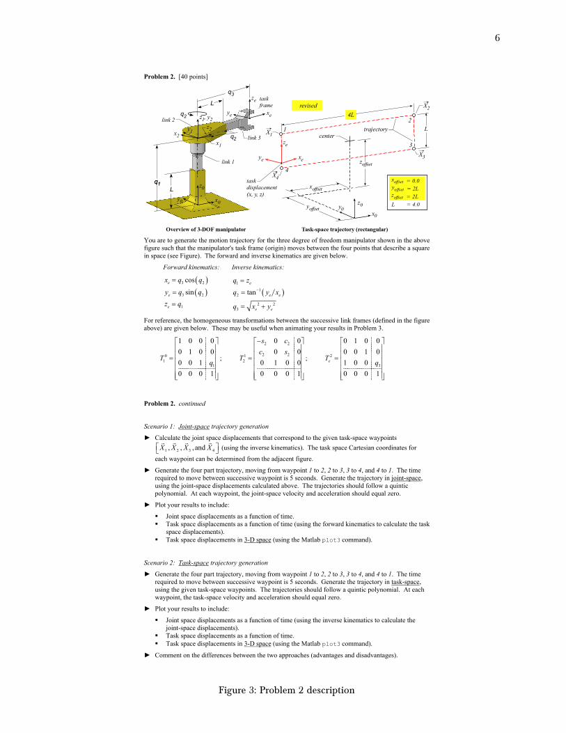
Problem 2. [40 points]

You are to generate the motion trajectory for the three degree of freedom manipulator shown in the above figure such that the manipulator's task frame (origin) moves between the four points that describe a square in space (see Figure). The forward and inverse kinematics are given below.

Forward kinematics: Inverse kinematics:

3 2

3 2

1

cos

sin

e

e

e

x q q

y q q

z q

1

12

2 23

tan

e

e e

e e

q z

q y x

q x y

For reference, the homogeneous transformations between the successive link frames (defined in the figure above) are given below. These may be useful when animating your results in Problem 3.

01

1

1 0 0 0

0 1 0 0

0 0 1

0 0 0 1

Tq

;

2 2

2 212

0 0

0 0

0 1 0 0

0 0 0 1

s c

c sT

; 2

3

0 1 0 0

0 0 1 0

1 0 0

0 0 0 1

eTq

Overview of 3-DOF manipulator

z0

y0 x0

q2

q2

q3

q1

taskframe

ze

ye xez1, y2

x2

x1

link 1

link 2

link 3

z2y1

q1L

L

ye xe

taskdisplacement(x, y, z)

ze

2

X2

4L

LX1

3

4

trajectory

X3

X4

1

z0y0x0

yoffset

zoffset

xoffset

center

L = 4.0

Task-space trajectory (rectangular)

xoffset = 0.0

zoffset = 2L

yoffset = 2L

revised

ME/ECE 739: Advanced Robotics Homework #4 Due: April 26th (Sunday, 11:59 pm)

Page 3 of 4

Problem 2. continued

Scenario 1: Joint-space trajectory generation

► Calculate the joint space displacements that correspond to the given task-space waypoints

1 2 3 4, , , andX X X X

(using the inverse kinematics). The task space Cartesian coordinates for

each waypoint can be determined from the adjacent figure.

► Generate the four part trajectory, moving from waypoint 1 to 2, 2 to 3, 3 to 4, and 4 to 1. The time required to move between successive waypoint is 5 seconds. Generate the trajectory in joint-space, using the joint-space displacements calculated above. The trajectories should follow a quintic polynomial. At each waypoint, the joint-space velocity and acceleration should equal zero.

► Plot your results to include:

Joint space displacements as a function of time. Task space displacements as a function of time (using the forward kinematics to calculate the task

space displacements). Task space displacements in 3-D space (using the Matlab plot3 command).

Scenario 2: Task-space trajectory generation

► Generate the four part trajectory, moving from waypoint 1 to 2, 2 to 3, 3 to 4, and 4 to 1. The time required to move between successive waypoint is 5 seconds. Generate the trajectory in task-space, using the given task-space waypoints. The trajectories should follow a quintic polynomial. At each waypoint, the task-space velocity and acceleration should equal zero.

► Plot your results to include:

Joint space displacements as a function of time (using the inverse kinematics to calculate the joint-space displacements).

Task space displacements as a function of time. Task space displacements in 3-D space (using the Matlab plot3 command).

► Comment on the differences between the two approaches (advantages and disadvantages).


7

The following 2D diagram illustrates the task space trajectory which is the path that the end e�ectorwill travel over.

L

2L

Ground level

End effector

1

34

z0

z offsetL

L/2

4L

L

2

q1

q3

problem_2_geometry.vsdxNasser M. Abbasi

4/16/2015

Figure 4: Problem 2 task path

0.2.1 First scenario

PART ONE:

The waypoints have the following coordinate values by inspection from the above diagram

𝑋1 = {−2𝐿, 2𝐿, 2.5𝐿}𝑋2 = {2𝐿, 2𝐿, 2.5𝐿}𝑋3 = {2𝐿, 2𝐿, 1.5𝐿}𝑋4 = {−2𝐿, 2𝐿, 1.5𝐿}

Inverse kinematics was used to determine the joint space displacements that corresponds to theabove task space. For 𝑋1 this results in

𝑞1 = 𝑧𝑒 = 2.5𝐿

𝑞2 = tan−1 �𝑦𝑒𝑥𝑒� = tan−1 �

2𝐿−2𝐿�

= 1350

𝑞3 = �𝑥2𝑒 + 𝑦2𝑒 = √4𝐿2 + 4𝐿2 = 2𝐿√2

For 𝑋2

𝑞1 = 𝑧𝑒 = 2.5𝐿


2𝐿2𝐿�

= 450

𝑞3 = �𝑥2𝑒 + 𝑦2𝑒 = √4𝐿2 + 4𝐿2 = 2𝐿√2

8

For 𝑋3

𝑞1 = 𝑧𝑒 = 1.5𝐿


2𝐿2𝐿�

= 450

𝑞3 = �𝑥2𝑒 + 𝑦2𝑒 = √4𝐿2 + 4𝐿2 = 2𝐿√2

And for 𝑋4

𝑞1 = 𝑧𝑒 = 1.5𝐿


2𝐿−2𝐿�

= 1350

𝑞3 = �𝑥2𝑒 + 𝑦2𝑒 = √4𝐿2 + 4𝐿2 = 2𝐿√2

PART TWO

The trajectory in joint space is now generated. The joint space coordinates was found above andillustrated in the following diagram

L

2L

Ground level

End effector

1

34

z0

z offset

L

L/2

4L

L

2

q1

q3

problem_2_geometry_joint_space.vsdxNasser M. Abbasi

4/16/2015

q1 2.5L

q2 1350

q3 2 2 L

q1 2.5L

q2 450

q3 2 2 L

q1 1.5L

q2 450

q3 2 2 L

q1 1.5L

q2 1350

q3 2 2 L

t 0 t 5sec

t 10sect 15sec

Figure 5: Problem 2 task path expressed in joint coordinates

A quintic polynomial was used with the restriction that at each waypoint �̇� = 0 and also �̈� = 0.

The above was done for each joint space path between two points. There are 3 joints. For each jointthe full path was generated. For example, for joint 𝑞1, the polynomial between 𝑋1 and 𝑋2 was foundby solving 6 equations in 6 unknowns. The polynomial is defined as

𝑞 (𝑡) = 𝑎0 + 𝑎1𝑡 + 𝑎2𝑡2 + 𝑎3𝑡3 + 𝑎4𝑡4 + 𝑎5𝑡5

9

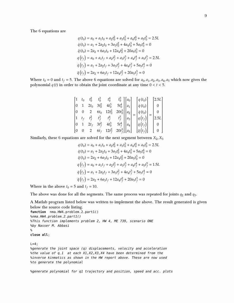
The 6 equations are

𝑞 (𝑡0) = 𝑎0 + 𝑎1𝑡0 + 𝑎2𝑡20 + 𝑎3𝑡30 + 𝑎4𝑡40 + 𝑎5𝑡50 = 2.5𝐿�̇� (𝑡0) = 𝑎1 + 2𝑎2𝑡0 + 3𝑎3𝑡20 + 4𝑎4𝑡30 + 5𝑎5𝑡40 = 0�̈� (𝑡0) = 2𝑎2 + 6𝑎3𝑡0 + 12𝑎4𝑡20 + 20𝑎5𝑡30 = 0

𝑞 �𝑡𝑓� = 𝑎0 + 𝑎1𝑡𝑓 + 𝑎2𝑡2𝑓 + 𝑎3𝑡3𝑓 + 𝑎4𝑡4𝑓 + 𝑎5𝑡5𝑓 = 2.5𝐿

�̇� �𝑡𝑓� = 𝑎1 + 2𝑎2𝑡𝑓 + 3𝑎3𝑡2𝑓 + 4𝑎4𝑡3𝑓 + 5𝑎5𝑡4𝑓 = 0

�̈� �𝑡𝑓� = 2𝑎2 + 6𝑎3𝑡𝑓 + 12𝑎4𝑡2𝑓 + 20𝑎5𝑡3𝑓 = 0

Where 𝑡0 = 0 and 𝑡𝑓 = 5. The above 6 equations are solved for 𝑎0, 𝑎1, 𝑎2, 𝑎3, 𝑎4, 𝑎5 which now gives thepolynomial 𝑞 (𝑡) in order to obtain the joint coordinate at any time 0 < 𝑡 < 5.

⎡⎢⎢⎢⎢⎢⎢⎢⎢⎢⎢⎢⎢⎢⎢⎢⎢⎢⎢⎢⎢⎢⎢⎢⎢⎣

1 𝑡0 𝑡20 𝑡30 𝑡40 𝑡500 1 2𝑡0 3𝑡20 4𝑡30 5𝑡400 0 2 6𝑡0 12𝑡20 20𝑡301 𝑡𝑓 𝑡2𝑓 𝑡3𝑓 𝑡4𝑓 𝑡5𝑓0 1 2𝑡𝑓 3𝑡2𝑓 4𝑡30 5𝑡4𝑓0 0 2 6𝑡𝑓 12𝑡2𝑓 20𝑡3𝑓

⎤⎥⎥⎥⎥⎥⎥⎥⎥⎥⎥⎥⎥⎥⎥⎥⎥⎥⎥⎥⎥⎥⎥⎥⎥⎦

⎡⎢⎢⎢⎢⎢⎢⎢⎢⎢⎢⎢⎢⎢⎢⎢⎢⎢⎢⎢⎢⎢⎢⎢⎢⎣

𝑎0𝑎1𝑎2𝑎3𝑎4𝑎5

⎤⎥⎥⎥⎥⎥⎥⎥⎥⎥⎥⎥⎥⎥⎥⎥⎥⎥⎥⎥⎥⎥⎥⎥⎥⎦

=

⎡⎢⎢⎢⎢⎢⎢⎢⎢⎢⎢⎢⎢⎢⎢⎢⎢⎢⎢⎢⎢⎢⎢⎢⎢⎣

𝑞 (𝑡0)�̇� (𝑡0)�̈� (𝑡0)𝑞 �𝑡𝑓��̇� �𝑡𝑓��̈� �𝑡𝑓�

⎤⎥⎥⎥⎥⎥⎥⎥⎥⎥⎥⎥⎥⎥⎥⎥⎥⎥⎥⎥⎥⎥⎥⎥⎥⎦

=

⎡⎢⎢⎢⎢⎢⎢⎢⎢⎢⎢⎢⎢⎢⎢⎢⎢⎢⎢⎢⎢⎢⎢⎢⎢⎣

2.5𝐿00

2.5𝐿00

⎤⎥⎥⎥⎥⎥⎥⎥⎥⎥⎥⎥⎥⎥⎥⎥⎥⎥⎥⎥⎥⎥⎥⎥⎥⎦

Similarly, these 6 equations are solved for the next segment between 𝑋2, 𝑋3

𝑞 (𝑡0) = 𝑎0 + 𝑎1𝑡0 + 𝑎2𝑡20 + 𝑎3𝑡30 + 𝑎4𝑡40 + 𝑎5𝑡50 = 2.5𝐿�̇� (𝑡0) = 𝑎1 + 2𝑎2𝑡0 + 3𝑎3𝑡20 + 4𝑎4𝑡30 + 5𝑎5𝑡40 = 0�̈� (𝑡0) = 2𝑎2 + 6𝑎3𝑡0 + 12𝑎4𝑡20 + 20𝑎5𝑡30 = 0

𝑞 �𝑡𝑓� = 𝑎0 + 𝑎1𝑡𝑓 + 𝑎2𝑡2𝑓 + 𝑎3𝑡3𝑓 + 𝑎4𝑡4𝑓 + 𝑎5𝑡5𝑓 = 1.5𝐿

�̇� �𝑡𝑓� = 𝑎1 + 2𝑎2𝑡𝑓 + 3𝑎3𝑡2𝑓 + 4𝑎4𝑡3𝑓 + 5𝑎5𝑡4𝑓 = 0

�̈� �𝑡𝑓� = 2𝑎2 + 6𝑎3𝑡𝑓 + 12𝑎4𝑡2𝑓 + 20𝑎5𝑡3𝑓 = 0

Where in the above 𝑡0 = 5 and 𝑡𝑓 = 10.

The above was done for all the segments. The same process was repeated for joints 𝑞2 and 𝑞3.

A Matlab program listed below was written to implement the above. The result generated is givenbelow the source code listing.function nma_HW4_problem_2_part1()%nma_HW4_problem_2_part1()%This function implements problem 2, HW 4, ME 739, scenario ONE%by Nasser M. Abbasi%close all;

L=4;%generate the joint space (q) displacements, velocity and acceleration%the value of q_1 at each X1,X2,X3,X4 have been determined from the%inverse kinmatics as shown in the HW report above. These are now used%to generate the polynomial

%generate polynomial for q1 trajectory and position, speed and acc. plots

10

figure;[t1,q1]=process_q(2.5*L,2.5*L,1.5*L,1.5*L,'q1',1.4*L,2.6*L,...

'meter','m/s','m/s^2');

%generate polynomial for q2 trajectory and position, speed and acc. plotsfigure;[t2,q2]=process_q(135*pi/180,45*pi/180,45*pi/180,135*pi/180,...

'q2',40*pi/180,155*pi/180,'angle(rad)','rad/sec','rad/sec^2');

%generate polynomial for q3 trajectory and position, speed and acc. plotsfigure;z=2*L*sqrt(2);[t3,q3]=process_q(z,z,z,z,'q3',0,1.2*2*L*sqrt(2),'meter','m/s','m/s^2');

%generate the task space X displacement using the forward kinematicsxe = q3.*cos(q2);ye = q3.*sin(q2);ze = q1;

%generate task space displacementsfigure;h1 = subplot(3,1,1);plot(t1,xe);title(h1,{'Task space displacements','Xe'});xlabel(h1,'time (sec)');ylabel(h1,'meter');axis(h1,[0 20 −2.2*L 2.2*L]);

h2 = subplot(3,1,2);plot(t2,ye);title(h2,'Ye');xlabel(h2,'time (sec)');ylabel(h2,'meter');axis(h2,[0 20 1.8*L 3*L]);

h3 = subplot(3,1,3);plot(t3,ze);title(h3,'Ze');xlabel(h3,'time (sec)');ylabel(h3,'meter');axis(h3,[0 20 1.4*L 2.6*L]);

%generate 3D plot of the task space trajectoryfigure;plot3(xe,ye,ze);hold on;plot3(−2*L,2*L,2.5*L,'o');text(−2*L,2*L,2.5*L,'X1');

plot3(2*L,2*L,2.5*L,'o');text(2*L,2*L,2.5*L,'X2');


11

plot3(−2*L,2*L,1.5*L,'o');text(−2*L,2*L,1.5*L,'X4');

plot3(0,2*L,2*L,'+');text(.1*L,2*L,2.1*L,'center');

title('3D task space displacement');xlabel('X'); ylabel('Y'); zlabel('Z');zlim([0 3*L]);

end%−−−−−−−−−−−−−−−−−−−−−−−function [t,q]=process_q(x1,x2,x3,x4,the_name,lim0,lim1,y1,y2,y3)%%Function to generate joint space trajectory for problem 2 for specific%joint q%x1: first point coordinate in this joint space%x2: second point coordinate in this joint space%x3: third point coordinate in this joint space%x4: fourth point coordinate in this joint space%the_name: title to put on the plot, for example 'q1' or 'q2' etc..%lim0 and lim1 are the y−axis limits to use for the plot%y1: position y label%y2: speed y label%y3: acceleration y label

%RETURNS%q: which is vector of q joint coordinates in joint space over%the full time space to be used later to generate the task space%trajectory using forward kinemetics%%t: the corresponding time vector

%call gen_path to obtain the polynomial coefficientsa = gen_path(x1,x2,0,5);[q1,dq,ddq,t1] = find_q(0,5,a); %use the coefficients to make polynomials[h1,h2,h3] = make_first_plot(t1,q1,dq,ddq);

title(h1,{the_name,'position'});title(h2,'velocity');title(h3,'acceleration');xlabel(h1,'time (sec)'); ylabel(h1,y1);xlabel(h2,'time (sec)'); ylabel(h2,y2);xlabel(h3,'time (sec)'); ylabel(h3,y3);

a = gen_path(x2,x3,5,10);[q2,dq,ddq,t2] = find_q(5,10,a);make_other_plot(t2,q2,dq,ddq,h1,h2,h3);


12


axis(h1,[0 20 lim0 lim1]);q=[q1 q2 q3 q4];t=[t1 t2 t3 t4];end

%−−−−−−−−−−−−−−−−−−−−−−−−−−−−−−−−−−−−−−−−−−−−−−function a = gen_path(q0,qf,t0,tf)%this function generates the polynomial coefficients by solving for the%constraints given

dq0 = 0;dqf = 0;ddq0 = 0;ddqf = 0;

C = [ 1 t0 t0^2 t0^3 t0^4 t0^5;0 1 2*t0 3*t0^2 4*t0^3 5*t0^4;0 0 2 6*t0 12*t0^2 20*t0^3;1 tf tf^2 tf^3 tf^4 tf^5;0 1 2*tf 3*tf^2 4*tf^3 5*tf^4;0 0 2 6*tf 12*tf^2 20*tf^3];

q = [q0 dq0 ddq0 qf dqf ddqf]';a = C\q;

end

%−−−−−−−−−−−−−−−−−−−−−−−−−−−−−−−−−−−−−−−−−−−−−−−−−function [q,dq,ddq,t]=find_q(t0,tf,a)%This function takes the coefficients of the polynomial and%return back the polynomials for position, speed and accelerationa0 = a(1); a1 = a(2); a2 = a(3); a3 = a(4); a4 = a(5); a5 = a(6);t = linspace(t0,tf,1000);q = a0 + a1*t + a2*t.^2 + a3*t.^3 + a4*t.^4 + a5*t.^5;dq = a1 + 2*a2*t + 3*a3*t.^2 + 4*a4*t.^3 + 5*a5*t.^4;ddq = 2*a2 + 6*a3*t + 12*a4*t.^2 + 20*a5*t.^3;

end

%−−−−−−−−−−−−−−−−−−−−−−−−−−−−−−−−−−−−−−−−−−−−−−−−−−−−−function [h1,h2,h3]=make_first_plot(t,q,dq,ddq)%this function plots the position in joint spaceh1 = subplot(3,1,1);plot(t,q)

h2 = subplot(3,1,2);plot(t,dq);

h3 = subplot(3,1,3);

13

plot(t,ddq);end

%−−−−−−−−−−−−−−−−−−−−−−−−−−−−−−−−−−−−−−−−−−−−−−−−function make_other_plot(t,q,dq,ddq,h1,h2,h3)%this function plots the speed and acceleration trajetory in joint spacehold(h1,'on');subplot(3,1,1);plot(t,q);plot(t(1),q(1),'o');

hold(h2,'on');subplot(3,1,2);plot(t,dq);plot(t(1),dq(1),'o');

hold(h3,'on');subplot(3,1,3);plot(t,ddq);plot(t(1),ddq(1),'o');end

time (sec)0 5 10 15 20

met

er

6

8

10

q1position

time (sec)0 5 10 15 20

m/s

-2

0

2velocity

time (sec)0 5 10 15 20

m/s

2

-1

0

1acceleration

Figure 6: Problem 2, part 1, 𝑞1 joint space trajectory

14

time (sec)0 5 10 15 20

angl

e(ra

d)

11.5

22.5

q2position

time (sec)0 5 10 15 20

rad/

sec

-1

0

1velocity

time (sec)0 5 10 15 20

rad/

sec2

-0.5

0

0.5acceleration

Figure 7: Problem 2, part 1, 𝑞2 joint space trajectory

time (sec)0 5 10 15 20

met

er

0

5

10

q3position

time (sec)0 5 10 15 20

m/s

-1

0

1velocity

time (sec)0 5 10 15 20

m/s

2

-1

0

1acceleration

Figure 8: Problem 2, part 1, task space 𝑥𝑒, 𝑦𝑒, 𝑧𝑒 trajectory

15

10

X2

X3

center

X

0

-10

X4

X1

3D task space displacement

89

Y

101112

8

10

12

2

0

6

4

Z

Figure 9: Problem 2, part 1, 3D plot of task space trajectory

0.2.2 Second scenario

The four part trajectory was generated again, using the same constraints as in first scenario, butnow the polynomial was generated in task space as required for this part. The polynomial betweenwaypoint 𝑋1 and 𝑋2 was found by solving 6 equations in 6 unknowns. The polynomial is defined foreach coordinate 𝑥𝑒, 𝑦𝑒, 𝑧𝑒. For example, for 𝑥𝑒

𝑥𝑒 (𝑡) = 𝑎0 + 𝑎1𝑡 + 𝑎2𝑡2 + 𝑎3𝑡3 + 𝑎4𝑡4 + 𝑎5𝑡5

The 6 equations are

𝑥𝑒 (𝑡0) = 𝑎0 + 𝑎1𝑡0 + 𝑎2𝑡20 + 𝑎3𝑡30 + 𝑎4𝑡40 + 𝑎5𝑡50 = 2.5𝐿�̇�𝑒 (𝑡0) = 𝑎1 + 2𝑎2𝑡0 + 3𝑎3𝑡20 + 4𝑎4𝑡30 + 5𝑎5𝑡40 = 0�̈�𝑒 (𝑡0) = 2𝑎2 + 6𝑎3𝑡0 + 12𝑎4𝑡20 + 20𝑎5𝑡30 = 0

𝑥𝑒 �𝑡𝑓� = 𝑎0 + 𝑎1𝑡𝑓 + 𝑎2𝑡2𝑓 + 𝑎3𝑡3𝑓 + 𝑎4𝑡4𝑓 + 𝑎5𝑡5𝑓 = 2.5𝐿

�̇�𝑒 �𝑡𝑓� = 𝑎1 + 2𝑎2𝑡𝑓 + 3𝑎3𝑡2𝑓 + 4𝑎4𝑡3𝑓 + 5𝑎5𝑡4𝑓 = 0

�̈�𝑒 �𝑡𝑓� = 2𝑎2 + 6𝑎3𝑡𝑓 + 12𝑎4𝑡2𝑓 + 20𝑎5𝑡3𝑓 = 0

Where 𝑡0 = 0 and 𝑡𝑓 = 5. The above 6 equations are solved for 𝑎0, 𝑎1, 𝑎2, 𝑎3, 𝑎4, 𝑎5 which gives thepolynomial 𝑥𝑒 (𝑡) used obtain the joint coordinate at any time 0 < 𝑡 < 5.

⎡⎢⎢⎢⎢⎢⎢⎢⎢⎢⎢⎢⎢⎢⎢⎢⎢⎢⎢⎢⎢⎢⎢⎢⎢⎣

1 𝑡0 𝑡20 𝑡30 𝑡40 𝑡500 1 2𝑡0 3𝑡20 4𝑡30 5𝑡400 0 2 6𝑡0 12𝑡20 20𝑡301 𝑡𝑓 𝑡2𝑓 𝑡3𝑓 𝑡4𝑓 𝑡5𝑓0 1 2𝑡𝑓 3𝑡2𝑓 4𝑡30 5𝑡4𝑓0 0 2 6𝑡𝑓 12𝑡2𝑓 20𝑡3𝑓

⎤⎥⎥⎥⎥⎥⎥⎥⎥⎥⎥⎥⎥⎥⎥⎥⎥⎥⎥⎥⎥⎥⎥⎥⎥⎦

⎡⎢⎢⎢⎢⎢⎢⎢⎢⎢⎢⎢⎢⎢⎢⎢⎢⎢⎢⎢⎢⎢⎢⎢⎢⎣

𝑎0𝑎1𝑎2𝑎3𝑎4𝑎5

⎤⎥⎥⎥⎥⎥⎥⎥⎥⎥⎥⎥⎥⎥⎥⎥⎥⎥⎥⎥⎥⎥⎥⎥⎥⎦

=

⎡⎢⎢⎢⎢⎢⎢⎢⎢⎢⎢⎢⎢⎢⎢⎢⎢⎢⎢⎢⎢⎢⎢⎢⎢⎣

𝑥𝑒 (𝑡0)�̇�𝑒 (𝑡0)�̈�𝑒 (𝑡0)𝑥𝑒 �𝑡𝑓��̇�𝑒 �𝑡𝑓��̈�𝑒 �𝑡𝑓�

⎤⎥⎥⎥⎥⎥⎥⎥⎥⎥⎥⎥⎥⎥⎥⎥⎥⎥⎥⎥⎥⎥⎥⎥⎥⎦

=

⎡⎢⎢⎢⎢⎢⎢⎢⎢⎢⎢⎢⎢⎢⎢⎢⎢⎢⎢⎢⎢⎢⎢⎢⎢⎣

2.5𝐿00

2.5𝐿00

⎤⎥⎥⎥⎥⎥⎥⎥⎥⎥⎥⎥⎥⎥⎥⎥⎥⎥⎥⎥⎥⎥⎥⎥⎥⎦

Similarly, these 6 equations were solved for the next segment between waypoint 𝑋2, 𝑋3. The sameprocess was repeated for 𝑦𝑒 and 𝑧𝑒.

16

The following gives the new Matlab implementation with the plots generated. Discussion on di�er-ences between the two approaches is given at the end.function nma_HW4_problem_2_part2()%nma_HW4_problem_2_part2()%This function implements problem 2, HW 4, ME 739, scenario TWO%by Nasser M. Abbasi%close all;

L=4;%generate the task space (X,Y,Z) displacements, velocity and acceleration%the value of x,y,z at each X1,X2,X3,X4 are given in the problem from%the diagram shown.

%generate polynomial for x−coodinate of each X waypoint trajectoryfigure;[t1,x_coordinate]=process_X(−2*L,2*L,2*L,−2*L,'x',−2.6*L,2.6*L,...

'meter','m/s','m/s^2');

%generate polynomial for y−coordinate of each X waypoint trajectoryfigure;[t2,y_coordinate]=process_X(2*L,2*L,2*L,2*L,...

'y',1.9*L,2.1*L,'meter','m/sec','m/sec^2');

%generate polynomial for z−coordinate of each X waypoint trajectoryfigure;[t3,z_coordinate]=process_X(2.5*L,2.5*L,1.5*L,1.5*L,'z',1.4*L,2.6*L,...

'meter','m/s','m/s^2');

%generate the corresponding joint space q displacement, speed and%acceleration from the above using forward kinematicsq1 = z_coordinate;q2 = atan2(y_coordinate,x_coordinate);q3 = sqrt(x_coordinate.^2+y_coordinate.^2);

%generate joint space displacementsfigure;h1 = subplot(3,1,1);plot(t1,q1);title(h1,{'Joint space displacements','q1'});xlabel(h1,'time (sec)');ylabel(h1,'meter');axis(h1,[0 20 0.9*L 2.8*L]);

h2 = subplot(3,1,2);plot(t2,q2);title(h2,'q2');xlabel(h2,'time (sec)');ylabel(h2,'radian');axis(h2,[0 20 30*pi/180 140*pi/180]);

h3 = subplot(3,1,3);plot(t3,q3);title(h3,'q3');

17

xlabel(h3,'time (sec)');ylabel(h3,'meter');axis(h3,[0 20 1.9*L 2.9*L]);

%generate 3D plot of the task space trajectoryfigure;plot3(x_coordinate,y_coordinate,z_coordinate);hold on;plot3(−2*L,2*L,2.5*L,'o');text(−2*L,2*L,2.5*L,'X1');



plot3(−2*L,2*L,1.5*L,'o');text(−2*L,2*L,1.5*L,'X4');

plot3(0,2*L,2*L,'+');text(.1*L,2*L,1.6*L,'center');

title('3D task space displacement');xlabel('X'); ylabel('Y'); zlabel('Z');zlim([0 3*L]);

end%−−−−−−−−−−−−−−−−−−−−−−−function [t,x]=process_X(x1,x2,x3,x4,the_name,lim0,lim1,y1,y2,y3)%%Function to generate task space trajectory for problem 2%x1: first point coordinate in this task space%x2: second point coordinate in this task space%x3: third point coordinate in this task space%x4: fourth point coordinate in this task space%the_name: title to put on the plot, for example 'x' or 'y' or 'z'%lim0 and lim1 are the y−axis limits to use for the plot%y1: position y label%y2: speed y label%y3: acceleration y label

%RETURNS%q: which is vector of q joint coordinates in joint space over%the full time space to be used later to generate the task space%trajectory using forward kinemetics%%t: the corresponding time vector

%call gen_path to obtain the polynomial coefficientsa = gen_path(x1,x2,0,5);[x_segment_1,dx,ddx,t1] = find_x(0,5,a); %use the coefficients to make polynomials[h1,h2,h3] = make_first_plot(t1,x_segment_1,dx,ddx);

18

title(h1,{the_name,'position'});title(h2,'velocity');title(h3,'acceleration');xlabel(h1,'time (sec)'); ylabel(h1,y1);xlabel(h2,'time (sec)'); ylabel(h2,y2);xlabel(h3,'time (sec)'); ylabel(h3,y3);

a = gen_path(x2,x3,5,10);[x_segment_2,dx,ddx,t2] = find_x(5,10,a);make_other_plot(t2,x_segment_2,dx,ddx,h1,h2,h3);



axis(h1,[0 20 lim0 lim1]);x=[x_segment_1 x_segment_2 x_segment_3 x_segment_4];t=[t1 t2 t3 t4];end

%−−−−−−−−−−−−−−−−−−−−−−−−−−−−−−−−−−−−−−−−−−−−−−function a = gen_path(x0,xf,t0,tf)%this function generates the polynomial coefficients by solving for the%constraints given

dx0 = 0;dxf = 0;ddx0 = 0;ddxf = 0;

C = [ 1 t0 t0^2 t0^3 t0^4 t0^5;0 1 2*t0 3*t0^2 4*t0^3 5*t0^4;0 0 2 6*t0 12*t0^2 20*t0^3;1 tf tf^2 tf^3 tf^4 tf^5;0 1 2*tf 3*tf^2 4*tf^3 5*tf^4;0 0 2 6*tf 12*tf^2 20*tf^3];

x = [x0 dx0 ddx0 xf dxf ddxf]';a = C\x;

end

%−−−−−−−−−−−−−−−−−−−−−−−−−−−−−−−−−−−−−−−−−−−−−−−−−function [x,dx,ddx,t]=find_x(t0,tf,a)%This function takes the coefficients of the polynomial and%return back the polynomials for position, speed and accelerationa0 = a(1); a1 = a(2); a2 = a(3); a3 = a(4); a4 = a(5); a5 = a(6);t = linspace(t0,tf,1000);x = a0 + a1*t + a2*t.^2 + a3*t.^3 + a4*t.^4 + a5*t.^5;

19

dx = a1 + 2*a2*t + 3*a3*t.^2 + 4*a4*t.^3 + 5*a5*t.^4;ddx = 2*a2 + 6*a3*t + 12*a4*t.^2 + 20*a5*t.^3;

end

%−−−−−−−−−−−−−−−−−−−−−−−−−−−−−−−−−−−−−−−−−−−−−−−−−−−−−function [h1,h2,h3]=make_first_plot(t,x,dx,ddx)%this function plots the position in task spaceh1 = subplot(3,1,1);plot(t,x)

h2 = subplot(3,1,2);plot(t,dx);

h3 = subplot(3,1,3);plot(t,ddx);end

%−−−−−−−−−−−−−−−−−−−−−−−−−−−−−−−−−−−−−−−−−−−−−−−−function make_other_plot(t,x,dx,ddx,h1,h2,h3)%this function plots the speed and acceleration trajetory in task spacehold(h1,'on');subplot(3,1,1);plot(t,x);plot(t(1),x(1),'o');

hold(h2,'on');subplot(3,1,2);plot(t,dx);plot(t(1),dx(1),'o');

hold(h3,'on');subplot(3,1,3);plot(t,ddx);plot(t(1),ddx(1),'o');end

20

time (sec)0 5 10 15 20

met

er

-10

0

10

xposition

time (sec)0 5 10 15 20

m/s

-10

0

10velocity

time (sec)0 5 10 15 20

m/s

2

-5

0

5acceleration

Figure 10: Problem 2, part 2, 𝑥𝑒 task space trajectory

time (sec)0 5 10 15 20

met

er

7.6

8

8.4

yposition

time (sec)0 5 10 15 20

m/s

ec

-1

0

1velocity

time (sec)0 5 10 15 20

m/s

ec2

-1

0

1acceleration

Figure 11: Problem 2, part 2, 𝑦𝑒 task space trajectory

21

time (sec)0 5 10 15 20

met

er

6

8

10

zposition

time (sec)0 5 10 15 20

m/s

-2

0

2velocity

time (sec)0 5 10 15 20

m/s

2

-1

0

1acceleration

Figure 12: Problem 2, part 2, 𝑧𝑒 task space trajectory

105

X2

X3

0

3D task space displacement

X-5

center

-107

X1

X4

7.5

Y

8

8.5

0

2

4

6

8

10

12

9

Z

Figure 13: Problem 2, part 2, 3D plot of task space trajectory

0.2.3 discussion

The following diagram gives an overview of the di�erence of the algorithm used for first and secondscenarios.

22

xetyetzet

xetyetzet

q1

q2

q3

q1tq2tq3t

Scenario one

X1

X2

X3

X4

Inverse kinematics applied to each way point

Joint space coordinate at each way point

Generate quintic trajectory polynomial between each way point in joint space

Plot joint space trajectories

Convert back to task space using forward kinematics

Plot 3D task space trajectory

q1tq2tq3t

Scenario two

X1

X2

X3

X4

Generate quintic trajectory polynomial between each way point in task space

Plot joint space trajectories

Plot 3D task space trajectory

Convert to joint space trajectory using inverse kinematics

Problem_2_final.vsdxNasser M. Abbasi

042315

Figure 14: Problem 2 algorithm di�erence scenario one and two

23

There are two main di�erences observed between the two methods.

1. In the first scenario, joint space trajectories 𝑞1(𝑡) and 𝑞2(𝑡) were the same as in the secondscenario, but 𝑞3(𝑡) was not the same.

In first scenario, 𝑞3(𝑡) was constant with value 2√2𝐿 for the whole path. This is becuase ateach way point 𝑞3 had the same value 2√2𝐿, therefore the polynomial generated was straightline connecting all the way points. In second scenario, 𝑞3(𝑡) was not constant, since 𝑞3(𝑡) =�𝑥𝑒(𝑡)2 + 𝑦𝑒(𝑡)2 and 𝑥𝑒(𝑡) polynomial was not constant (even though 𝑦𝑒(𝑡) was constant over thewhole path).

2. In the first scenario, 𝑦𝑒(𝑡) was generated by inverse kinematics using 𝑦𝑒(𝑡) = 𝑞3(𝑡) sin(𝑞2(𝑡)) andeven though 𝑞3(𝑡) was constant, 𝑞2(𝑡) was not. Hence the path along the 𝑦 direction is task spacewas changing as can be seen from the above plot. In the second scenario, since the 𝑦 was fixedat each way point, the trajectory generated in task space shows that 𝑦(𝑡) is not changing. This iswhy the 3D plot for the second scenario do not show the same curved path in the 𝑦 dimensionas in the first scenario.

The result from first scenario seems to be more realistic 3D task space path that the robot arm ende�ector would take. Computationally, there is little di�erence between the two scenarios.

0.3 Problem 3ME/ECE 739: Advanced Robotics Homework #4 Due: April 26th (Sunday, 11:59 pm)

Page 4 of 4

Problem 3. [40 points]

For the manipulator described in Problem 2

► Use a parabolic well potential to define an attractive field applied to the origin of frame {e}. Use Matlab to implement a gradient descent algorithm to find a path from the specified initial configuration to the specified final configuration given below. Initial configuration: 0 0

Tq L L

Final configuration: 122 2

T

fq L L

► Animate your results using the Matlab rendering functions posted to the Learn@UW course page.

In general, you can vary i (the scaling factor applied to the attractive force, fi) to modify the resulting path. In this case, the forces are applied at only one point so there is only one value of . You can also vary the gradient descent scaling factor, . Larger values of can speed up the gradient descent algorithm, but can also cause numerical instabilities in the solution. In addition, you can use different values of (i for joint i) to scale the joint torques and thus modify the path solution.

Gradient descent:

1

1

kf

k k

while q q

q q U

k k

where

k

k

qU

q

and

1 0

0 n

► Vary i and comment on the resulting solution behavior (both in regards to the shape of the path and the numerical stability of the solution.


In this problem we need to determine only the attractive virtual force on origin of end e�ectorframe {e}. The repulsive forces are not involved. The attractive virtual forces are approximated witha parabolic well potential. We have only one location where the force is applied to (which is theorigin of frame {e}, which is the end e�ector). The first step is to determine the virtual force from

24

the gradient of the parabolic potential field given by

𝑭𝑒 = −∇𝑈𝑒

= −𝜁 �𝒐𝑒 �𝑞𝑐𝑢𝑟𝑟𝑒𝑛𝑡� − 𝒐𝑒 �𝑞𝑓��

Where in the above 𝒐𝑒 �𝑞� is the position vector of the origin of frame {e} at current configuration

𝑞 and 𝒐𝑒 �𝑞𝑓� is position vector of the origin of frame {e} at final configuration 𝑞𝑓. Hence 𝒐𝑒 �𝑞𝑓� isconstant position vector and only 𝒐𝑒 �𝑞� will change as the robot arm moves.

We are given the final configuration as 𝑞𝑓 = �2𝐿, 𝜋2 , 2𝐿�𝑇, and we now use this to obtain 𝒐𝑒 �𝑞𝑓�. We

first need to obtain 𝑇0𝑒 which we obtained forward kinematics given in problem 2. Hence

𝑇0𝑒 = 𝑇0

1𝑇12𝑇2

𝑒

=

⎡⎢⎢⎢⎢⎢⎢⎢⎢⎢⎢⎢⎢⎢⎢⎣

1 0 0 00 1 0 00 0 1 𝑞10 0 0 1

⎤⎥⎥⎥⎥⎥⎥⎥⎥⎥⎥⎥⎥⎥⎥⎦

⎡⎢⎢⎢⎢⎢⎢⎢⎢⎢⎢⎢⎢⎢⎢⎣

− sin 𝑞2 0 cos 𝑞2 0cos 𝑞2 0 sin 𝑞2 00 1 0 00 0 0 1

⎤⎥⎥⎥⎥⎥⎥⎥⎥⎥⎥⎥⎥⎥⎥⎦

⎡⎢⎢⎢⎢⎢⎢⎢⎢⎢⎢⎢⎢⎢⎢⎣

0 1 0 00 0 1 01 0 0 𝑞30 0 0 1

⎤⎥⎥⎥⎥⎥⎥⎥⎥⎥⎥⎥⎥⎥⎥⎦

=

⎡⎢⎢⎢⎢⎢⎢⎢⎢⎢⎢⎢⎢⎢⎢⎣

cos 𝑞2 − sin 𝑞2 0 𝑞3 cos 𝑞2sin 𝑞2 cos 𝑞2 0 𝑞3 sin 𝑞20 0 1 𝑞10 0 0 1

⎤⎥⎥⎥⎥⎥⎥⎥⎥⎥⎥⎥⎥⎥⎥⎦

Therefore, 𝒐𝑒 �𝑞� from the above is the last column. Hence

𝒐𝑒 �𝑞𝑐𝑢𝑟𝑟𝑒𝑛𝑡� =

⎡⎢⎢⎢⎢⎢⎢⎢⎢⎢⎣

𝑞3 cos 𝑞2𝑞3 sin 𝑞2

𝑞1

⎤⎥⎥⎥⎥⎥⎥⎥⎥⎥⎦

We now replace the values of 𝑞1, 𝑞2, 𝑞3 in the above, with the final configuration values given

𝒐𝑒 �𝑞𝑓𝑖𝑛𝑎𝑙� =

⎡⎢⎢⎢⎢⎢⎢⎢⎢⎢⎣

2𝐿 cos 𝜋2

2𝐿 sin 𝜋2

2𝐿

⎤⎥⎥⎥⎥⎥⎥⎥⎥⎥⎦=

⎡⎢⎢⎢⎢⎢⎢⎢⎢⎢⎣

02𝐿2𝐿

⎤⎥⎥⎥⎥⎥⎥⎥⎥⎥⎦

And the initial configuration (at time 𝑡 = 0) is

𝒐𝑒 �𝑞𝑖𝑛𝑖𝑡𝑖𝑎𝑙� =

⎡⎢⎢⎢⎢⎢⎢⎢⎢⎢⎣

𝐿 cos 0𝐿 sin 0

𝐿

⎤⎥⎥⎥⎥⎥⎥⎥⎥⎥⎦=

⎡⎢⎢⎢⎢⎢⎢⎢⎢⎢⎣

𝐿0𝐿

⎤⎥⎥⎥⎥⎥⎥⎥⎥⎥⎦

Using the above, we need determine the virtual force 𝐹𝑒

25

𝑭𝑒 = −∇𝑈𝑒

= −𝜁𝑒 �𝒐𝑒 �𝑞𝑐𝑢𝑟𝑟𝑒𝑛𝑡� − 𝒐𝑒 �𝑞𝑓��

= −𝜁𝑒

⎛⎜⎜⎜⎜⎜⎜⎜⎜⎜⎝

⎡⎢⎢⎢⎢⎢⎢⎢⎢⎢⎣

𝑞3 cos 𝑞2𝑞3 sin 𝑞2

𝑞1

⎤⎥⎥⎥⎥⎥⎥⎥⎥⎥⎦−

⎡⎢⎢⎢⎢⎢⎢⎢⎢⎢⎣

02𝐿2𝐿

⎤⎥⎥⎥⎥⎥⎥⎥⎥⎥⎦

⎞⎟⎟⎟⎟⎟⎟⎟⎟⎟⎠

= −𝜁𝑒

⎡⎢⎢⎢⎢⎢⎢⎢⎢⎢⎣

𝑞3 cos �𝑞2�𝑞3 sin 𝑞2 − 2𝐿

𝑞1 − 2𝐿

⎤⎥⎥⎥⎥⎥⎥⎥⎥⎥⎦

In the above, all the 𝑞𝑖 variables are the current joint variables at the current time. In simulation,there will change with time. Now that we found the virtual force, we convert it to joint toque usingthe linear velocity Jacobian. We obtain 𝐽𝑣𝑒 by direct di�erentiation method

𝐽𝑣𝑒 =

⎡⎢⎢⎢⎢⎢⎢⎢⎢⎢⎢⎢⎢⎣

𝜕𝑥𝜕𝑞1

𝜕𝑥𝜕𝑞2

𝜕𝑥𝜕𝑞3

𝜕𝑦𝜕𝑞1

𝜕𝑦𝜕𝑞2

𝜕𝑦𝜕𝑞3

𝜕𝑧𝜕𝑞1

𝜕𝑧𝜕𝑞2

𝜕𝑧𝜕𝑞3

⎤⎥⎥⎥⎥⎥⎥⎥⎥⎥⎥⎥⎥⎦

From problem 2, we are given that

𝑥𝑒 = 𝑞3 cos 𝑞2𝑦𝑒 = 𝑞3 sin 𝑞2𝑧𝑒 = 𝑞1

Hence 𝐽𝑣𝑒 becomes

𝐽𝑣𝑒 =

⎡⎢⎢⎢⎢⎢⎢⎢⎢⎢⎢⎢⎣

𝜕 𝑞3 cos 𝑞2𝜕𝑞1



𝜕 𝑞3 sin 𝑞2𝜕𝑞1



𝜕𝑞1𝜕𝑞1

𝜕𝑞1𝜕𝑞2

𝜕𝑞1𝜕𝑞3

⎤⎥⎥⎥⎥⎥⎥⎥⎥⎥⎥⎥⎦=

⎡⎢⎢⎢⎢⎢⎢⎢⎢⎢⎣

0 −𝑞3 sin 𝑞2 cos 𝑞20 𝑞3 cos 𝑞2 sin 𝑞21 0 0

⎤⎥⎥⎥⎥⎥⎥⎥⎥⎥⎦

Therefore, using the duality relation that 𝜏 = ∑ 𝐽𝑇𝑣𝑖𝐹𝑖 and since we have forces on one joint only, thissimplifies to 𝜏 = 𝐽𝑇𝑣𝑒𝐹𝑒

𝝉 = −𝜁𝑒

⎡⎢⎢⎢⎢⎢⎢⎢⎢⎢⎣

0 −𝑞3 sin 𝑞2 cos 𝑞20 𝑞3 cos 𝑞2 sin 𝑞21 0 0

⎤⎥⎥⎥⎥⎥⎥⎥⎥⎥⎦

𝑇 ⎡⎢⎢⎢⎢⎢⎢⎢⎢⎢⎣

𝑞3 cos �𝑞2�𝑞3 sin 𝑞2 − 2𝐿

𝑞1 − 2𝐿

⎤⎥⎥⎥⎥⎥⎥⎥⎥⎥⎦

= −𝜁𝑒

⎡⎢⎢⎢⎢⎢⎢⎢⎢⎢⎣

𝑞1 − 2𝐿𝑞3 �cos 𝑞2� �𝑞3 sin 𝑞2 − 2𝐿� − 𝑞23 cos 𝑞2 sin 𝑞2

𝑞3 cos2 𝑞2 + �sin 𝑞2� �𝑞3 sin 𝑞2 − 2𝐿�

⎤⎥⎥⎥⎥⎥⎥⎥⎥⎥⎦

(1)

26

The above is the actual torque/force applied at the joints 1,2 and 3. Therefore, the force applied tojoint 1 is 𝑞1 − 2𝐿 and the torque to apply to joint 2 is 𝑞3 �cos 𝑞2� �𝑞3 sin 𝑞2 − 2𝐿� − 𝑞23 cos 𝑞2 sin 𝑞2 and the

force to apply to end e�ector joint is 𝑞3 cos2 𝑞2 + �sin 𝑞2� �𝑞3 sin 𝑞2 − 2𝐿� .

For example, at initial configuration, where 𝑞𝑖𝑛𝑖𝑡𝑖𝑎𝑙 = [𝐿, 0, 𝐿]𝑇 we find

𝝉𝑖𝑛𝑖𝑡𝑖𝑎𝑙 = −𝜁𝑒

⎡⎢⎢⎢⎢⎢⎢⎢⎢⎢⎣

−𝐿−2𝐿𝑞3𝐿

⎤⎥⎥⎥⎥⎥⎥⎥⎥⎥⎦

And at final configuration where 𝑞𝑓𝑖𝑛𝑎𝑙 = 𝑞𝑓 = �2𝐿, 𝜋2 , 2𝐿�𝑇we find

𝝉𝑖𝑛𝑖𝑡𝑖𝑎𝑙 = −𝜁𝑒

⎡⎢⎢⎢⎢⎢⎢⎢⎢⎢⎣

000

⎤⎥⎥⎥⎥⎥⎥⎥⎥⎥⎦

Which is what we would expect. At the final configuration, the applied forces at the joints shouldvanish since we have arrived at the final configuration.

Now that we have equation (1), we can use it to implement the gradient descent algorithm in orderto obtain the sequence of 𝑞𝑖 positions to use for the animation.

0.3.1 Part one

In this part, a single 𝛼 value was used for all the joints. This value was changed in order to observethe a�ect. In second part below, di�erent 𝛼 for each joint will be used.

In this part, and in all runs, 𝜁 was set to 100. This is the attractive force scaling value.

Below is the source code written to implement this part of the problem. The following diagram showsthe initial configuration for one example run.

27

step = 1, position=[4.00,0.00,4.00], alpha=0.015, epsilon=0.005

5

0

x-5

-5y

0

5

0

2

4

6

8

10

z

Figure 16: Initial configuration, problem 3

And the following diagram shows the final configuration reached. It shows that it took 535 steps toreach the final configuration using 𝛼 = 0.015 and 𝜖 = 0.005

Figure 17: Final configuration, problem 3

As 𝛼 was made smaller the convergence became slower, but the animation became more accurateand ran more smoothly. As the end e�ector came very close to the target, more vibration aroundthat region started to show as the end e�ector oscillated around the target point as it converged tothe exact target and the error became smaller and smaller.

To run the program, the command is nma_HW4_problem_3function nma_HW4_problem_3()%function nma_HW4_problem_3()%This function implements path planning for the 3 links robot arm in

28

%HW4, ME 739, problem 3, spring 2015, Univ. Wiscosin, Madison.%%This version is for part 1, which uses one alpha for all joints%%Parabolic attractive field is used to model the attractive virtual%force on the end effector. The linear velocity Jacobian is used to%map this force to torque forces at the three joints.%Then gradient descent is used to obtain the joint coordinates sequence%which is then used to simulate the motion.%%By Nasser M. Abbasi

close all; clear all;L = 4; %length of link 1 and 3%epsilon = 0.005; %error tolerance%alpha = 0.015; %smaller value, slows down convergence but more accurate

epsilon = 0.05; %error tolerancezeta = 100; %attractive force scalingalpha = 0.05; %smaller value, slows down convergence but more accurate

q = [L;0;L]; %initial joint configurationqf = [2*L;pi/2;2*L]; %find joint configurationmaxIter = 1200; %max iterations allowed

Q = zeros(3,maxIter); %where to save the sequence of joint q'sk = 1;keep_running = true;

%start of gradient descemt

while keep_runningQ(:,k) = q;tau = −zeta*[q(1)−2*L;

q(3)*cos(q(2))*(q(3)*sin(q(2))−2*L)−q(3)^2*cos(q(2))*sin(q(2));q(3)*(cos(q(2)))^2+sin(q(2))*(q(3)*sin(q(2))−2*L)];

q = q + alpha*tau/norm(tau);if k+1>maxIter || norm( q−qf ) <= epsilon

keep_running = false;else

k = k +1;end

end

DO_MOVIE = false; %make true to generate movie framesframeNumber = 0;

f_handle = 1;axis_limits = L*[−2 2 −2 2 −0.1 2.5];render_view = [−.4 −.8 .5]; view_up = [0 0 1];SetRenderingViewParameters(axis_limits,render_view,view_up,f_handle);camproj perspective % turns on perspective

29

% link 0 rendering initializationr0 = L/5; sides0 = 4; axis0 = 3; norm_L0 = −1.0;linkColor0 = [0 .3 .3]; plotFrame0 = 0;d0 = CreateLinkRendering(L,r0,sides0,axis0,norm_L0,linkColor0,...

plotFrame0,f_handle);

% link 1 rendering initializationr1 = L/6; sides1 = 4; axis1 = 3; norm_L1 = 1.0;linkColor1 = [0 0.75 0]; plotFrame1 = 0;d1 = CreateLinkRendering(L,r1,sides1,axis1,norm_L1,linkColor1,...


% link 2 rendering initializationr2 = L/7; sides2 = 10; axis2 = 3; norm_L2 = −1.0;linkColor2 = [0.75 0 0]; plotFrame2 = 0;d2 = CreateLinkRendering(L,r2,sides2,axis2,norm_L2,linkColor2,...


% link 3 rendering initializationr3 = L/8; sides3 = 4; axis3 = 1; norm_L3 = 1.0;linkColor2 = [0.75 0 1]; plotFrame2 = 0;d3 = CreateLinkRendering(L,r3,sides3,axis3,norm_L3,linkColor2,...


T00 = [1 0 0 00 1 0 00 0 1 00 0 0 1];

UpdateLink(d1,T00);

for i = 1:k% Update framesq1=Q(1,i); q2=Q(2,i); q3=Q(3,i);T01 = [1 0 0 0

0 1 0 00 0 1 q10 0 0 1];

T12 = [−sin(q2) 0 cos(q2) 0cos(q2) 0 sin(q2) 00 1 0 00 0 0 1];

T2e = [0 1 0 00 0 1 01 0 0 q30 0 0 1];

T02 = T01*T12;T0e = T02*T2e;

UpdateLink(d1,T01);UpdateLink(d2,T02);

30

UpdateLink(d3,T0e);

title(sprintf('step = %d, position=[%3.2f,%3.2f,%3.2f], alpha=%3.3f, epsilon=%3.3f',i,...q3*cos(q2),q3*sin(q2),q1,alpha,epsilon));

%if i == 1; %pause at start of simulation rendering% pause;%end

if DO_MOVIEframeNumber = frameNumber+1;I = getframe(gcf);imwrite(I.cdata, sprintf('frame%d.png',frameNumber));

endhold on;plot3(0,2*L,2*L,'marker','o','color','r');drawnow;hold off;pause(0.01);

endend

0.3.2 Part two

In this part, di�erent 𝛼𝑖 values were used for each joint. The code to implement this part is similarto the above with the only change is in using a diagonal matrix for 𝛼 instead of justone scalar value.Di�erent 𝛼𝑖 was used for each joint to see the e�ect on the path of the end e�ector.

The following vector of values gave the best solution

alpha = diag([0.05,0.01,0.1]);

The above produced the least amount of oscillation as the end e�ector came close to the target.Making 𝛼𝑖 smaller caused the joint 𝑖 to move the slowest during the animation.

The following value of vector 𝛼 caused large oscillation as the end e�ector came close to the target.

alpha = diag([0.05,0.1,0.01]);

These values of 𝛼 are kept in the code below to allow one to try them. The source code for thispart is listed below. Using di�erent 𝛼𝑖 value for each joint is more flexible and allowed findingbetter solution than using the same 𝑎𝑙𝑝ℎ𝑎 for all joints. The command to run the Matlab script isnma_HW4_problem_3_part2function nma_HW4_problem_3_part2()%function nma_HW4_problem_3_part2()%This function implements path planning for the 3 links robot arm in%HW4, ME 739, problem 3, spring 2015, Univ. Wiscosin, Madison.%%This version is for part 2, which uses different alpha for each joint%%Parabolic attractive field is used to model the attractive virtual%force on the end effector. The linear velocity Jacobian is used to%map this force to torque forces at the three joints.

31

%Then gradient descent is used to obtain the joint coordinates sequence%which is then used to simulate the motion.%%By Nasser M. Abbasi

close all; clear all;L = 4; %length of link 1 and 3%epsilon = 0.005; %error tolerance%alpha = 0.015; %smaller value, slows down convergence but more accurate

epsilon = 0.01; %error tolerancezeta = 100; %attractive force scaling%alpha = diag([0.05,0.1,0.01]); %Causes large errors in solutionalpha = diag([0.05,0.01,0.1]); %Produces best solution

q = [L;0;L]; %initial joint configurationqf = [2*L;pi/2;2*L]; %find joint configurationmaxIter = 1000; %max iterations allowed

Q = zeros(3,maxIter); %where to save the sequence of joint q'sk = 1;keep_running = true;

%start of gradient descemt

while keep_runningQ(:,k) = q;tau = −zeta*[q(1)−2*L;

q(3)*cos(q(2))*(q(3)*sin(q(2))−2*L)−q(3)^2*cos(q(2))*sin(q(2));q(3)*(cos(q(2)))^2+sin(q(2))*(q(3)*sin(q(2))−2*L)];

q = q + alpha*tau/norm(tau);if k+1>maxIter || norm( q−qf ) <= epsilon

keep_running = false;else

k = k +1;end

end

DO_MOVIE = false; %make true to generate movie framesframeNumber = 0;

f_handle = 1;axis_limits = L*[−2 2 −2 2 −0.1 2.5];render_view = [−.4 −.8 .5]; view_up = [0 0 1];SetRenderingViewParameters(axis_limits,render_view,view_up,f_handle);camproj perspective % turns on perspective

% link 0 rendering initializationr0 = L/5; sides0 = 4; axis0 = 3; norm_L0 = −1.0;linkColor0 = [0 .3 .3]; plotFrame0 = 0;d0 = CreateLinkRendering(L,r0,sides0,axis0,norm_L0,linkColor0,...


32

% link 1 rendering initializationr1 = L/6; sides1 = 4; axis1 = 3; norm_L1 = 1.0;linkColor1 = [0 0.75 0]; plotFrame1 = 0;d1 = CreateLinkRendering(L,r1,sides1,axis1,norm_L1,linkColor1,...


% link 2 rendering initializationr2 = L/7; sides2 = 10; axis2 = 3; norm_L2 = −1.0;linkColor2 = [0.75 0 0]; plotFrame2 = 0;d2 = CreateLinkRendering(L,r2,sides2,axis2,norm_L2,linkColor2,...


% link 3 rendering initializationr3 = L/8; sides3 = 4; axis3 = 1; norm_L3 = 1.0;linkColor2 = [0.75 0 1]; plotFrame2 = 0;d3 = CreateLinkRendering(L,r3,sides3,axis3,norm_L3,linkColor2,...


T00 = [1 0 0 00 1 0 00 0 1 00 0 0 1];

UpdateLink(d1,T00);

for i = 1:k% Update framesq1=Q(1,i); q2=Q(2,i); q3=Q(3,i);T01 = [1 0 0 0

0 1 0 00 0 1 q10 0 0 1];

T12 = [−sin(q2) 0 cos(q2) 0cos(q2) 0 sin(q2) 00 1 0 00 0 0 1];

T2e = [0 1 0 00 0 1 01 0 0 q30 0 0 1];

T02 = T01*T12;T0e = T02*T2e;

UpdateLink(d1,T01);UpdateLink(d2,T02);UpdateLink(d3,T0e);

title(sprintf('step = %d, position=[%3.2f,%3.2f,%3.2f], epsilon=%3.3f',i,...q3*cos(q2),q3*sin(q2),q1,epsilon));

%if i == 1; %pause at start of simulation rendering% pause;

33

%end

if DO_MOVIEframeNumber = frameNumber+1;I = getframe(gcf);imwrite(I.cdata, sprintf('frame%d.png',frameNumber));

endhold on;plot3(0,2*L,2*L,'marker','o','color','r');drawnow;hold off;pause(0.01);

endend

Documents

HW4 ME 739 Introduction to robotics