HUB-EP-98/57

THE MECHANISM OF QUARK CONFINEMENT

Gunnar S. Bali∗

Institut fur Physik, Humboldt Universitat, Invalidenstraße 110, 10115 Berlin,Germany

ABSTRACT

I summarise recent lattice results on the QCD confinement mechanism in themaximally Abelian projection.

1. Introduction

The phenomenology of strong interactions contains two fundamental ingredients:asymptotic freedom and the confinement of colour charges. The former requirement ledto the invention of QCD. A mathematically rigorous proof that QCD as the microscopictheory of strong interactions indeed gives rise to the macroscopic property of linearquark confinement as indicated by Regge trajectories and quarkonia spectra is, aftera quarter of a century, still lacking. Meanwhile, lattice gauge theory simulations haveprovided convincing numerical evidence for this conjecture.

The difficulty in deriving infra red properties of QCD illustrates that somethingqualitatively new is happening: unlike in previously existing elementary physical theo-ries, it is not possible to reduce everything down to two-body interactions but collectiveexcitations of quark and gluon states have to be accounted for. For the first time, ex-citations of the vacuum that are considered to be fundamental do not occur as initialor final states anymore. Therefore, understanding confinement, in my opinion, is one ofthe most exciting challenges of modern physics. New physical and mathematical tech-niques that can successfully be applied to non-perturbative QCD might be requiredfor dealing with other strongly interacting theories or theories with a non-trivial vac-uum structure, in general. Vice versa techniques developed in a different context mighthelp to prove QCD confinement and in solving QCD. A recent example is the proofof confinement in SUSY Yang-Mills theories.1 Of course QCD as we know it does notobey super-symmetry but nonetheless such activities point into a promising direction.Just as QCD can serve as a guinea pig and development centre for non-perturbativetechniques, lattice simulations help probing the validity range of effective low-energymodels or in verifying certain conjectures.

QCD in itself is sufficiently complicated to keep many physicists busy. SolvingQCD is still important and even more so since (almost) everyone believes in it. Itis widely accepted that perturbative QCD (pQCD) successfully describes high en-ergy scattering processes. However, without understanding non-perturbative aspects

∗Talk given at 3rd International Conference on Quark Confinement and Hadron Spectrum (Confine-ment III), Newport News, VA, 7-12 Jun 1998.

of QCD, even in this case, it is not clear why pQCD works at all. Only hadrons, lep-tons and photons but no quarks or gluons are observed in experiment. In order tofill the gap, the formation of colour-neutral hadronic jets from quarks and gluons hasto be modelled. Furthermore, it is commonly conjectured that, once the fundamentalscattering on the quark and gluon level has taken place, further interactions can beneglected. It is demanding to derive the ingredients of fragmentation models directlyfrom truly non-perturbative QCD, as well as to verify the factorisation hypothesis.

Many phenomenologically important questions are posed in low-energy QCD thateagerly await an answer: is the same set of fundamental parameters (QCD coupling andquark masses) that describes for instance the hadron spectrum consistent with highenergy QCD or is there place for new physics? Are all hadronic states correctly classifiedby the naıve quark model or do glueballs, hybrid states and molecules play a role? Atwhat temperatures/densities does the transition to a quark-gluon plasma occur? Whatare the experimental signatures of quark-gluon matter? Can we solve nuclear physicson the quark and gluon level? Clearly, complex systems like iron nuclei are unlikelyever to be solved from first principles alone but modelling and certain approximationswill always be required. Therefore, it is desirable to test model assumptions, to gaincontrol over approximations and, eventually, to derive low-energy effective Lagrangiansfrom QCD. Lattice simulations are a very promising tool for this purpose.

In the past decades, many explanations of the confinement mechanism have beenproposed, most of which share the feature that topological excitations of the vacuumplay a major role. A list of these theories includes the dual superconductor picture ofconfinement,2,3 the centre vortex model,4 the instanton liquid model,5 and the anti-ferromagnetic vacuum.6 All these interpretations have been explored in lattice studies.The situation with respect to an anti-ferromagnetic vacuum is still somewhat incon-clusive.7 Instantons seem to be more vital for chiral symmetry related properties thanfor confinement.8 Depending on the picture, the excitations giving rise to confinementare thought to be magnetic monopoles, instantons, dyons, centre vortices, etc.. I wouldlike to stress that the above ideas are not completely disjoint and do not necessarilyexclude each other. For instance, all the above mentioned topological excitations arefound to be correlated with each other in numerical as well as analytical studies.

I will restrict myself to the, at present, most popular superconductor picture whichis based on the concept of electro-magnetic duality after an Abelian gauge projection.Recently, the centre vortex model has been resuscitated too. In the latter picture,the centre group that is directly related to the traditional order parameter of the de-confinement phase transition in finite temperature pure gauge theories, the Polyakovline, plays an essential role. Another striking feature is that — unlike monopole cur-rents — centre vortices form two-dimensional objects, such that in four space-timedimensions, a linking number between a Wegner-Wilson loop and centre vortices canunambiguously be defined, providing a geometric interpretation of the confinementmechanism.9 Unfortunately, I have not enough space to review these exciting develop-ments. Therefore, I refer the interested reader to a review by Greensite.10

Another obvious omission are questions related to chiral properties of QCD. Realworld QCD is not only a theory of gluons but includes quarks which means that the de-confinement phase transition will eventually be replaced by a chiral phase transition. In

the phase with broken chiral symmetry colour charges are still being anti-screened andlinear confinement approximately holds. However, if the binding energy within a hadronexceeds a critical value, the hadron will break up into two or more colour-neutral parts(string breaking).

Based on different confinement pictures various effective models of infra red QCDhave been proposed in the past. Three such examples are the Abelian Higgs model,11,9

the stochastic vacuum model12 and dual QCD.13 As well as understanding the mecha-nism of confinement, it is desirable to verify aspects of these models and eventually toderive certain model parameters directly from QCD.

This article is organised as follows. I will start with a brief motivation and in-troduction into lattice methods in Sec. 2, before explaining the concept of the Abelianprojection in Sec. 3. Subsequently, I will introduce some notations and review latticeresults in Sec. 4 and conclude with a summary of answered and open questions.

2. Why Lattice?

Lattice methods allow for a somewhat brute force but first principles numericalevaluation of expectation values of a given quantum field theory that is defined by anaction S. The lattice volume and spacing are limited due to finite computer speed andmemory. Simulations are performed in Euclidean space and an analytic continuationto Minkowski space of numerical results that have been obtained on discrete pointswith finite precision is virtually impossible. Therefore, not every physically meaningfulquantity can be calculated in a straight forward manner. The obvious strength of latticemethods are hadron mass determinations. Even if one is unimpressed by post-dictionsof experimental values that have been known with high precision for decades, withinan accuracy of only 5 %, such simulations allow one to fix fundamental standard modelparameters like quark masses and QCD running coupling in the low-energy domain.Of course, plenty of other applications of phenomenological importance exist.

Unfortunately, only the lowest lying one or two radial excitations of a hadronicstate are accessible in practice. Lattice predictions are restricted to rather simple sys-tems too. Even the deuterium is beyond the reach of present day super-computers.Therefore, it is desirable to supplement lattice simulations by analytical methods. Thecomputer alone acts as a black box. In order to understand and interprete the outputvalues and to predict their dependence on the input parameters, some modelling isrequired. Vice versa, the lattice itself is a strong tool to validate models and approx-imations. Unlike in the “real” world, we can vary the quark masses mi

q, the numberof colours Nc, the number of flavours nf , the temperature, the volume, the space-timedimension of our femto-universe and even the boundary conditions in order to exposemodels to thorough tests in many situations. Instead of indirectly and in a somewhatuncontrolled fashion deriving parameter values from experiment we can compute cus-tom designed observables. What is thought to work in the real world ought to work onthe lattice too! Moreover, many models rely on certain approximations. Experimental-ists cannot switch off quark flavours but we can!

In a lattice simulation, hyper-cubic Euclidean space-time is discretised on a boxwith, say, L4 lattice points or sites, x. Two adjacent points are connected by an orientedbond or link (x, µ). The product of four links, enclosing an elementary square, is a

plaquette. Quarks are living on sites, gauge fields on links and the plaquette determinesthe curvature within the SU(Nc) group manifold and corresponds to the field strengthtensor. For simplicity, we assume an isotropic lattice with equal lattice spacing a in alldirections. The lattice spacing provides an ultra violet cut-off on the gluon momentaq < π/a and regulates the theory.

We simulate an action S(β,miq) on the lattice, which contains the quark masses

as well as an inverse QCD coupling β = 2Nc/g2 as free parameters. By varying β (and

miq) the lattice spacing a is changed. Asymptotic freedom tells us that the ultra violet

cut-off is removed as β →∞. The physical dimension of a is determined by calculatinga dimensionful quantity on the lattice and associating it to its experimental value. If theright theory is being simulated we should be able to reproduce all experimental massratios in the continuum limit a→ 0, such that it becomes irrelevant what experimentalquantity we have chosen to set the scale∗. In practice one does not get all the quarkmasses right, such that there are always systematic uncertainties in a, due to theambiguity of the choice of this experimental input quantity.

The discretised lattice action is formulated in a manifestly gauge-invariant wayand approaches the continuum action with a→ 0. One ideally extrapolates to this limitat fixed physical lattice extent, La = const.. Later on, the thermodynamic limit La→∞ should be investigated. Due to the finiteness of a computer these two extrapolations,as well as extrapolations and interpolations between results obtained at different quarkmasses, are subject to systematic uncertainties that have to be carefully estimated.For most hadronic processes, a lattice spacing a < 0.1 fm is considered to be close tothe continuum limit while an extent La ≈ 2 fm is comfortably large to accommodateground state mesons and baryons.

Expectation values of operators O are determined by computation of the pathintegral,

〈O〉 =1

Z

∫[dU ][dψ][dψ]O[U ]e−S[U,ψ,ψ]. (1)

The normalisation factor Z is such that 〈1〉 = 1. Ux,µ ∈ SU(Nc) denotes a gaugefield and the 4 × nf × Nc tuple ψx is a fermion field. The high-dimensional integralis evaluated by means of a (stochastic) Monte-Carlo method as an average over anensemble of n representative gauge configurations, Ci = U (i)

x,µ, i = 1, . . . , n. Therefore,the result on the expectation value is subject to a statistical error that will basicallydecrease like 1/

√n: the longer we measure the more precise the prediction becomes.

Therefore, we might speak of lattice measurements and lattice experiments in analogyto “real” experiments. Ideally, the sample size n is such that the statistical precision issimilar or smaller than the systematic uncertainty of the extrapolations.

In Fig. 1 I illustrate that confinement is a numerical fact by displaying the poten-tial between a static quark and an anti-quark, separated by a distance r. The data havebeen obtained in SU(3) gauge theory with and without two light (mass-degenerate)

∗In the results presented here, I set the scale (somewhat arbitrarily) by the value√σ = 440 MeV for

the string tension in case of SU(2) and by the value r0 = 0.5 fm in case of SU(3) chromodynamics. r0is the distance at which r2

0 dV (r)/dr|r0 = 1.65 where V (r) denotes the potential between two static

colour sources, separated by a distance r.

-3

-2

-1

0

1

2

3

0.5 1 1.5 2 2.5 3

[V(r

)-V

(r0]

r 0

r/r0

quenchedκ = 0.1575

Fig. 1. Ground state (full symbols) and Eu hybrid potential (open symbols) at β = 6.2(quenched) and β = 5.6, κ = 0.1575.14

quark flavours at lattice spacings somewhat smaller than 0.1 fm. The scale r0 corre-sponds to 0.5 fm. The (partially) unquenched potential, that has been obtained at aquark mass mq ≈ 50 MeV, exhibits a more pronounced singularity at small r, due to theslower running of the QCD coupling towards zero as the momentum scale is increased(or r is decreased). Furthermore, from r ≈ 1.2 fm onwards, the (partially) unquenchedpotential eventually flattens: the QCD string “breaks”. Indeed, many interesting fea-tures of the theory can be studied on the lattice that are not at all accessible to realexperiment. As an example, I have included a so-called Eu (or continuum Πu) hybridpotential15,16 into the plot that corresponds to the interaction energy of two staticquark sources for the case that gluons contribute one unit of angular momentum alongthe interquark axis.

3. (Abelian) photons and monopoles

Soon after the advent of QCD, ’t Hooft and Mandelstam2 proposed the dualsuperconductor scenario of confinement; the QCD vacuum is thought to behave analo-gously to an electrodynamic superconductor but with the roles of electric and magneticfields being interchanged: a condensate of magnetic monopoles expels electric fields fromthe vacuum. If one now puts electric charge and anti-charge into this medium, the elec-tric flux that forms between them will be squeezed into a thin, eventually string-like,Abrikosov-Nielsen-Oleson (ANO) vortex which results in linear confinement.

In all quantum field theories in which confinement has been proven, namely incompact U(1) gauge theory in the Villain formulation,17 the Georgi-Glashow model18

and SUSY Yang-Mills theories,1 this scenario is indeed realised. Before one can ap-ply this picture to QCD or SU(Nc) chromodynamics one has to identify the relevantdynamical variables: it is not straight forward to generalise the electro-magnetic du-ality of a U(1) gauge theory to SU(Nc) since gluons carry colour charges. How can

one define electric fields in a gauge invariant way? What fields are dual to the electricfields? How can one identify a monopole current? The next question is that for theorder parameter of the confinement-deconfinement phase transition: what symmetryis broken? One might also ask why this symmetry is broken — a question that hasbeen answered by the BCS theory for conventional superconductors. Finally, we areinterested in an effective low-energy theory which corresponds to the Ginzburg-Landautheory of standard superconductors.

Let us address the first question. In the Georgi-Glashow model, the SO(3) gaugesymmetry is broken down to a U(1) symmetry as the vacuum expectation value ofthe Higgs field becomes finite. Within this effective U(1) theory, the standard electro-magnetic duality is realised, resulting in confinement. Such a mechanism is not providedby QCD but one can attempt to reduce the SU(Nc) symmetry to an Abelian symmetryby hand. In this spirit, it has been proposed3 to identify the monopoles in the U(1)Nc−1

diagonal Cartan subgroup of SU(Nc) gauge theory after gauge fixing in respect to theoff-diagonal SU(Nc)/U(1)Nc−1 degrees of freedom (Abelian projection).

In general, a gauge transformation, Ωx ∈ SU(Nc)/U(1)Nc−1, can be found thatdiagonalises an arbitrary operator Xx = f [UΩ] within the adjoint representation ofSU(Nc) when applied to the link variables,

UΩx,µ = ΩxUx,µΩ†x+aµ. (2)

Subsequently, a coset decomposition of the gauge transformed links is performed,

UΩx,µ = Cx,µux,µ with Cx,µ ∈ SU(Nc)/U(1)Nc−1, ux,µ ∈ U(1)Nc−1. (3)

If we now apply a residual gauge transformation, ωx ∈ U(1)Nc−1, we find,

ux,µ −→ ωxux,µω†x+aµ, Cx,µ −→ ωxux,µω

†x, (4)

i.e. ux,µ transforms like a gauge field while Cx,µ transform like matter fields. Therefore,we will refer to the diagonal gluon field ux,µ as “photon” field. While the gauge fieldsof electrodynamics in the non-compact continuum formulation are free of singularitiesand, therefore, cannot form magnetic monopole solutions, the gauge transformation Ωx

is singular wherever two eigenvalues of Xx coincide. Therefore, the gauge field ux,µ willin general contain such monopoles.

After Abelian gauge fixing QCD can be regarded as a theory of interacting pho-tons, monopoles and matter fields (i.e. off-diagonal gluons and quarks). One might as-sume that the off-diagonal gluons do not affect long range interactions. This conjectureis known as Abelian dominance.19 In addition, monopole dominance of non-perturbativephysics has been proposed.20

The identification of photon fields and monopoles is a gauge invariant process.However, the choice of the operator Xx, that defines the Abelian projection, is am-biguous. In his original work, ‘t Hooft suggested that the dual superconductor sce-nario would be realised in any Abelian projection. Indeed, the expectation value ofa monopole creation operator has been found to be an order parameter of the de-confinement phase transition in quite a few different projections of SU(2) chromody-namics.21 As long as any U(1)Nc−1 projection of the theory yields similar results, one

does not have to specify the mechanism that is thought to break the SU(Nc) gaugesymmetry of QCD. However, numerical simulations suggest that Abelian and monopoledominance are not at all universal. The most popular gauge projection applied and dis-cussed is the maximally Abelian projection (MAP).3 One feature that is not sharedby almost all other projections that have been investigated on the lattice so far is thatthe (local) MAP gauge condition gives rise to non-propagating ghost fields only, guar-anteeing renormalisability of the Abelian projected theory. Another — and possiblyrelated — fact is that both, Abelian and monopole dominance have qualitatively beenverified in this projection.

One should mention that the analogy to an ordinary superconductor after Abelianprojection is not complete. The electrons that form Cooper pairs in BCS theory are allnegatively charged. However, the monopoles that are thought to condense in QCD cancarry both, negative and positive magnetic charges. Therefore, the composition of thecondensate is very different. The origin of the interaction that results in an attractiveforce between monopoles and anti-monopoles also differs from the periodic backgroundpotentials of the BCS theory.

I will briefly explain how MAP is performed on the lattice for the case of SU(2)gauge theory. In the first step one maximises the functional,22

F (Ω) =∑x,µ

tr(τ3U

Ωx,µτ3U

Ω†x,µ

), (5)

by means of a gauge transformation Ωx. τ3 denotes a Pauli-matrix†. After the max-imisation, all link variables are as diagonal as possible. The resulting gauge fields

UΩx,µ = exp

(i∑cA

cx,µτc/2

)satisfy ’t Hooft’s differential MA gauge fixing condition,3

(∂µ ± iA

3x,µ

)A±x,µ = 0, A±x,µ =

1√

2

(A1x,µ ±A

2x,µ

). (6)

After gauge fixing, the projection is performed: observables are calculated onAbelian configurations θx,µ rather than Ux,µ. We refer to the field theory, definedin this way, as Abelian projected SU(2) gauge theory [APSU(2)]. For convenience theAbelian links are represented in the Lie algebra rather than the group itself, ux,µ =exp (iθx,µτ3). Note that the normalisation has been chosen such that the periodicity ofθµ is 2π as opposed to the periodicity 4π of A3

µ. With this convention we find magneticcharges to be multiples of 2π/e just like in electrodynamics rather than 2Ncπ/e as onemight have expected in SU(Nc) gauge theory. We also use the convention e = 1 for thefundamental electric charge.

Recently, some articles have appeared whose authors claim to have “proven”Abelian dominance, either in general or specifically in the MAP. In one case the argu-ment is based on the fact that the off-diagonal gluon fields acquire mass and, therefore,

†In principle, we can fix the gauge along any direction within the SU(2) group space. The resultinggauges will only differ from each other by a global gauge transformation that will not affect expectationvalues — as long as we perform the subsequent coset decomposition with respect to the same U(1)subgroup. Also note that if we forced an adjoint Higgs field with a δ-like potential into the 3-direction,the form of the interaction term with the gauge fields would be identical to F .

are thought to affect ultra violet physics only, a statement that does not necessarily ap-ply to confining field theories. Other arguments are either based on misinterpretationsof the transfer matrix formalism or on rewriting the original theory in terms of Abelianprojected variables plus perturbations (the off-diagonal fields) that are proportionalto a small parameter ε. In order to avoid going too much into details I only mentionthat both, the static potential and Wilson loops in MAP are very different from theircounter parts in the original theory, even for large distances. In case of the potential,the asymptotic slope (string tension) comes out to be similar. However, APSU(2) andSU(2) potentials are shifted with respect to each other by a substantial constant dueto different self-energy contributions. Any “proof” that fails to account for the latterfact is necessarily wrong to some extent.

4. Results

4.1. Some Definitions

The language of differential forms23 turns out to be very convenient for the presentpurpose and this is even more so on the lattice. Let us start with a U(1) field theoryin D = 4 dimensions. The anti-symmetric field strength tensor F (a 2-form) can bedecomposed as follows,

F = dA+ δ∗C, (7)

where A denotes the standard magnetic four-potential (1-form) and C denotes anelectric four-potential which is a 1-form on the dual lattice. A and C are not uniquelydetermined but subject to a Uel(1)×Umag(1) gauge invariance since gradients of scalarfields can be added. “d” denotes the exterior derivative that, applied to an n-form,results in an n + 1-form. “∗” is the pull-back operator that connects an n-form toa (D − n)-form on the dual lattice while the dual derivative δ = ∗d∗ turns n-formsinto (n − 1)-forms. We have ∗2 = 1 and d2 = δ2 = 0. We define a Laplacian 2 =(−)D(dδ + δd).

In this notation, we obtain the generalised Maxwell equations,

δF = j, dF = ∗k. (8)

The electric current j is a 1-form on the original lattice while the magnetic (monopole)current k is a 1-form on the dual lattice. In Landau gauge (δA = 0 or δC = 0,respectively) this means,

j = 2A, k = 2C. (9)

Note that, unlike the continuum four-potential A, the link angles θ ∈ (−π, π] aresubject to a 2π shift-periodicity. Therefore, the identification,

F =1

a2sin (dθ)

[1 +O(a2)

], (10)

is natural for electro-magnetic fields. We can factorise the plaquette dθ ∈ (−4π, 4π]into a regular part θ2 ∈ (−π, π] and a singular part m ∈ −2,−1, 0, 1, 2:

dθ = θ2 + 2πm. (11)

While ddθ = 0, dθ2 = −2πdm does not necessarily vanish. Let us consider the magneticflux through a (spatial) plaquette, Φmag = a2dθ [1 +O(a2)], which, in the absenceof monopole strings, would be identical to a contour integral of the vector potentialA around the plaquette. However, in presence of monopoles, only exp (i

∫2d

2f dθ) =exp (i

∫∂2dxA) holds: the argument can be shifted by multiples of 2π which, with

the normalisation e = 1, is the elementary monopole charge. Thus, −2πm countsthe monopole contribution to the magnetic flux through the plaquette and −2πdmcorresponds to the “flux” out of a 3-cube, such that24

k = −2π ∗dm = ∗dθ2 (12)

is a magnetic monopole current‡. k is conserved since δk = −2πδ2∗m = 0, i.e. monopolecurrents form closed loops on the dual lattice. The individual components of k can takevalues 2πn with n = −4,−3, . . . , 4.

Monopole currents can alternatively be defined through,25 k = ∗dF = ∗d sin (dθ),the advantage being that the second Maxwell equation [Eq. (8)] is automatically ful-

filled. The current k is obviously conserved too. The quantisation of magnetic charges,however, is obscured by lattice artefacts. Magnetic monopoles become extended objectsand a geometric interpretation is not as straight forward as for the definition presentedbefore. For all results I am going to review, the first definition has been used. Note thatthe locations of monopoles in either of the definitions are not necessarily identical topositions of singularities of the adjoint operator X that has been diagonalised by thegauge fixing, as originally proposed by ’t Hooft.

Each link variable can be factorised26–28 into a singular part θsing that is inducedby magnetic monopoles and a regular (or photon) part θreg = θ − θsing that obeysthe homogenous Maxwell equation dF = d sin(dθreg) = 0. If we take the divergence ofEq. (11) in Landau gauge (δθ = 0) we obtain,

2πδm = δdθ = 2θsing. (13)

One solution of this equation is obviously,

θsingx = −2π∑y

Dxyδmy, (14)

where Dxy denotes the lattice Coulomb propagator in position space.Instead of using the Abelian links θx,µ one can evaluate observables from the

monopole and photon parts θsingx,µ and θregx,µ, separately. We will refer to such expec-tation values as monopole and photon contributions, respectively.

4.2. Successes

I will present some facts in support of the superconductor confinement scenario inthe MAP: approximate Abelian dominance of the static potential has been verified.20

In a recent study on a large lattice,26 the APSU(2) string tension has been confirmed

‡I assume the quantities to be given in lattice units a. k has dimension a−3, F has dimension a−2.

0

0.1

0.2

0.3

0.4

0.5

0.6

0.7

0.8

2 4 6 8 10 12 14 16

aV(r

)

r/a

VAb

Vreg

Vsing

Vsing+Vreg

Fig. 2. Photon and monopole contributions V reg and V sing to the APSU(2) potential26 V Ab

in units a ≈ 0.081 fm.

to account for (92 ± 4)% of the SU(2) string tension. It is an open question whetherthe agreement will improve as the continuum limit is approached.

The photon part of the potential does not contain a linear contribution. Monopoledominance and the factorisation V Ab(r) = V sing(r) + V reg(r) approximately hold. InFig. 2, we display the result of a recent lattice study.26 Everything is plotted in latticeunits a ≈ 0.081 fm. The monopole contribution amounts to (95± 1)% of the Abelianstring tension.

Approximate Abelian and monopole dominance has been confirmed for the lighthadron spectrum29 of SU(3) gauge theory. In Fig. 3, I display recent results on thenucleon and ρ masses that have been obtained on a lattice with extent La ≈ 2.8 fmand spacing a ≈ 0.175 fm. On the horizontal axis, the squared pion mass (in unitsof the string tension) is displayed, which changes as the quark mass is varied. Resultsfor SU(3), APSU(3) and Abelian monopole contributions as well as for SU(3) withthe photon part removed lie on the same curve. In the same study, π and ρ massesare found to become degenerate, as soon as the monopole contribution to the gaugefields is subtracted, both in SU(3) chromodynamics and the Abelian projected theory,i.e. Abelian monopoles are required for chiral symmetry breaking. Consistent resultshave been found by Lee et al.27 and Bielefeld et al..30 Of course, one can also arguethat since instantons are always accompanied by Abelian monopoles,31 removing thesemonopoles naturally results in a trivial vacuum topology.

The one-loop β-functions in APSU(Nc) and SU(Nc) gauge theories agree,32 i.e. atweak coupling, masses obtained in both theories should be proportional to each other.A recent analytical investigation has also confirmed anti-screening of colour fields inAPSU(2).33 These results are in agreement with numerical data.26,34

For the next few observations, I refer to M. Polikarpov’s talk at this conference:

0.0 1.0 2.0 3.0 4.0 5.0mπ

2/σ

0.0

1.0

2.0

3.0

4.0

5.0

m/σ

1/2

SU(3)APSU(3)monopoleSU(3)-photon

ρ meson

proton

Fig. 3. SU(3) ρ and nucleon masses: Abelian, monopole and non-photon contributions.29

monopoles have been found to be condensed in the confined phase of SU(2) gaugetheory.21,35 Furthermore, APSU(2) monopoles are spatially correlated with regions ofaccess in the SU(2) action density36 which rules out that the monopoles are meregauge fixing artefacts since their presence is reflected in gauge invariant observables.An effective monopole Lagrangian has been constructed which can (approximately) bemapped onto the Abelian Higgs model.9

4.3. Puzzles

Of course, we do not expect SU(Nc) gauge theories to be identical to an AbelianHiggs model. So, we should become suspicious if the picture did not fail to describe theQCD reality at some point. Obviously, APSU(2) becomes very different from SU(2)gauge theory in the ultra violet. I will restrict myself to two points where somethingin the infra red might go wrong that I consider as being serious.

The static potential between sources within the adjoint representation of SU(2)(adjoint potential) will saturate at a distance at which the binding energy exceeds thegluelump-gluelump threshold.15 Therefore, we expect for the adjoint string tension σadjthe asymptotic value,

σadj = limr→∞

dVadj(r)

dr= 0. (15)

In APSU(2) we obtain for adjoint Wilson loops around a rectangle S,

WAbadj(S) =

1

3

[1 + 2WAb,2(S)

], WAb,2 = cos

2∑

(x,µ)∈∂S

θx,µ

, (16)

where we call WAb,2 the charge two Wilson loop; the adjoint source corresponds toa neutral and two charge two Abelian components. Obviously, as the area S goes to

-0.5

0

0.5

1

1.5

2 4 6 8 10 12 14 16

aV(r

)

r/a

VAb,2(R)-VAb,20

expectationVAb(R)-VAb

0

Fig. 4. The charge two potential in APSU(2) in lattice units a ≈ 0.081 fm.26

infinity, WAbadj(S) approaches the constant value 1/3. Therefore,

V Abadj =

1

alimt→∞

logW (r, t)

W (r, t+ a)= 0 ∀ r, (17)

i.e. the correct asymptotic value σAbadj = 0 is produced.However, lattice results indicate that the adjoint string will only break deep in

the infra red at a distance slightly smaller than 1.5 fm,15 a region in which we wouldexpect Abelian dominance to hold if we consider the MAP theory to have relevance forhadronic physics. Simple models predict a linear rise of the potential in the intermediateregion, with a slope that is proportional to the Casimir charge of the representation, i.e.σadj = 8/3 σ for SU(2) gauge theory. Indeed, lattice simulations yield a linear increase,however with slightly smaller slope: 2σ ≤ σadj < 8/3 σ. In Fig. 4 the fundamentalpotential V Ab(r) is displayed, together with the charge two potential V Ab,2(r).26 Thecurves are fits in accord to the parametrisation,

V Ab(,2)(r) = −eAb(,2)

r+ σAb(,2)r. (18)

The upmost curve corresponds to eAb,2 = 4eAb, σAb,2 = 8/3 σAb. As in SU(2), we findthe slope in APSU(2) to be somewhat smaller than expected.

In conclusion, it seems that the charge two potential resembles the features ofthe adjoint potential within SU(2). However, it is not clear how we can get rid of theneutral contribution to the adjoint Wilson loop. For this purpose, interactions with theoff-diagonal gluons have to be considered.

A second puzzle that has recently been noticed34 is related to the energy dis-tribution within the ANO vortex between static sources. In Fig. 5, I show the 1/e

0

0.2

0.4

0.6

0.8

1

1.2

1.4

0 0.5 1 1.5 2 2.5 3 3.5 4 4.5

δ 1/e

σ1/2

r σ1/2

SU(2) actionAPSU(2) action

APSU(2) energyclassical dipole

Fig. 5. 1/e-radius of the flux tube in SU(2) and APSU(2).34

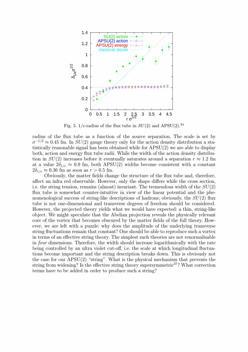
radius of the flux tube as a function of the source separation. The scale is set byσ−1/2 ≈ 0.45 fm. In SU(2) gauge theory only for the action density distribution a sta-tistically reasonable signal has been obtained while for APSU(2) we are able to displayboth, action and energy flux tube radii. While the width of the action density distribu-tion in SU(2) increases before it eventually saturates around a separation r ≈ 1.2 fmat a value 2δ1/e ≈ 0.9 fm, both APSU(2) widths become consistent with a constant2δ1/e ≈ 0.36 fm as soon as r > 0.5 fm.

Obviously, the matter fields change the structure of the flux tube and, therefore,affect an infra red observable. However, only the shape differs while the cross section,i.e. the string tension, remains (almost) invariant. The tremendous width of the SU(2)flux tube is somewhat counter-intuitive in view of the linear potential and the phe-nomenological success of string-like descriptions of hadrons; obviously, the SU(2) fluxtube is not one-dimensional and transverse degrees of freedom should be considered.However, the projected theory yields what we would have expected: a thin, string-likeobject. We might speculate that the Abelian projection reveals the physically relevantcore of the vortex that becomes obscured by the matter fields of the full theory. How-ever, we are left with a puzzle: why does the amplitude of the underlying transversestring fluctuations remain that constant? One should be able to reproduce such a vortexin terms of an effective string theory. The simplest such theories are not renormalisablein four dimensions. Therefore, the width should increase logarithmically with the ratebeing controlled by an ultra violet cut-off, i.e. the scale at which longitudinal fluctua-tions become important and the string description breaks down. This is obviously notthe case for our APSU(2) “string”. What is the physical mechanism that prevents thestring from widening? Is the effective string theory supersymmetric37? What correctionterms have to be added in order to produce such a string?

d

*δ

ρ

ρ

E, j H= *B

B, kD= *E

original lattice

dual lattice

0-form 1-form 2-form 3-form

el

mag

Fig. 6. Differential forms in D = 3 dimensions.

-6

-4

-2

0

2

4

6

-15 -10 -5 0 5 10 15

-4

-2

0

2

4

-4 -2 0 2 4

Fig. 7. Electric field E and magnetic super current k between two static sources.

4.4. The Dual Superconductor in Detail

In order to obtain an effective low-energy Lagrangian with monopoles and photonsas fundamental degrees of freedom one can attempt to determine the free parametersby numerically matching the effective action to that of APSU(2).9,20 To complementsuch studies, one might probe the APSU(2) vacuum with electric (or magnetic) testcharges to verify predictions of the effective theory and measure the values of themodel parameters, which is the line I am going to follow here. Investigations of fielddistributions in presence of charges have been performed previously.38 I will concentrateon the results from a more recent study.39

We are probing the vacuum with static electric sources. For this purpose weconsider three dimensional spatial cross sections (time slices) of the lattice. In Fig. 6,I have visualised where on the lattice different objects are “living”. The advantage inworking with differential forms is that the Stokes theorem is guaranteed to be exactand not subject to lattice artefacts: if the differential Maxwell equations are fulfilled,

the integrated versions automatically hold too. Of course, when finally relating latticeresults to continuum physics, lattice artefacts re-enter the game. The (generalised)Maxwell equations [Eq. (8)] read,

δE = ρel, dE = ∗k− ∗B, (19)

δB = ρmag , dB = ∗j + ∗E. (20)

The charge densities ρel and ρmag are the 4-components of j and k, respectively. The“dot”-symbol denotes a temporal derivative. For a static problem, electric and magneticfields decouple. In the absence of magnetic test charges, this implies ρmag = 0, j = 0and, therefore, B = 0 such that we are left with two Maxwell equations only, δE = ρeland dE = ∗k.

As mentioned above, one can define the monopole current via the latter equa-tion (Ampere’s law) which is then trivially fulfilled. However, with our definition of k[Eq. (12)] neither of the equations necessarily holds. Strong fields may give rise to non-linear quantum corrections. Moreover, APSU(2) is not electrodynamics; in general, theaction will be non-local and the equations of motion might differ. Our numerical study,however, verifies div E to disappear outside of the vicinity of the sources while the curlof the electric field is identical to the magnetic current.39 I display the electric fieldfor a distance r = 15a ≈ 1.2 fm in Fig. 7. The vortex is stabilised by the surroundingsuper current k.

The starting point of our investigation is the London limit. The electric vectorpotential C on the dual lattice is defined through,

E = ∗dC. (21)

One representation of the (dual) London equations reads,

C + λ2k = 0, (22)

with λ being the inverse mass of the dual photon. By building the curl of this relation,we obtain E = −λ2 ∗ dk which, together with the dual Ampere law results in,

E = −λ2δdE = λ2(∇2E + dρel

). (23)

Without an electric current j, the Maxwell equations imply, d(B + λ2dk

)= 0, i.e.

even in the absence of a magnetic field, the super current k remains constant andin general non-zero. From Eq. (23) it is also obvious why λ is called the penetrationlength: if we expose a superconducting probe to a homogeneous electric field, E = Ezex,the field strength will decay with the distance x towards the centre of the medium:Ez(x) = Ez(0) exp(−x/λ).

We create a charge-anticharge pair at a separation r parallel to the z-axis of ourlattice, ρel = δ3(−r/2 ez)− δ3(r/2 ez). x denotes the transverse distance from the coreof the ANO vortex. For the electric flux through any surface enclosing the charge, weexpect Φel =

∫d2xEz(x, 0) = 1. For our geometry Eq. (23) reads in the centre plane

perpendicular to the vortex,

Ez(x) = λ2∇22Ez(x) + Φδ2(x), Ex(x) = 0. (24)

A solution can be expressed in terms of the modified Bessel function K0,

Ez(x) =Φel

2πλ2K0(x/λ). (25)

Within statistical accuracy, we find our data to be compatible with such a functional

form for x > xmin = 4.2a ≈ 0.35 fm§ with parameter values,

λ = (1.82± 0.07)a ≈ (1.3 GeV)−1, Φel = 1.44± 0.08. (26)

For small x the data are overestimated by the fit since K0(x) diverges as x→ 0 whichexplains why the electric flux comes out to be significantly larger than one. A dualphoton mass of 1.3 GeV is compatible with the mass of the lightest glueball in SU(2)gauge theory. However, the quantum numbers of a dual photon are JPC = 1+− asopposed to 0+ for this glueball.

How can we refine our description such that the electric field not only in thesurface region but also closer to the centre of the vortex is correctly reproduced? Obvi-ously, a second scale ξ that is smaller than the 0.035 fm, above which the London limitseems to apply, has to be introduced. Such a scale appears in the Ginzburg-Landau(GL) equations as the coherence length of the GL wave function ψ(x) that describes thespatial density of superconducting monopole charges, n(x) = |ψ(x)|2. We decomposeψ into a phase and an amplitude f ,

ψ(x) = ψ∞f(x)eiθ(x), f(x)x→∞−→ 1. (27)

ξ characterises the decay of the monopole density towards the centre of the vortex,where f will vanish as superconductivity breaks down, while λ controls the penetrationof the vortex field into the surrounding vacuum. The case ξ = 0 corresponds to theLondon limit. If we increase the width of the flux tube, the dia-electric energy of thevortex is reduced by an amount roughly in proportion to λE2 while the amount ofenergy we have to pay for pushing the monopoles further into the vacuum increaseslike ξE2. Values ξ <

√2λ correspond to a negative surface energy in accord to the

Abrikosov criterium for a classical system. This tendency to maximise the surfaceresults in retardation of flux tubes: we obtain a type II superconductor while valuesκ = λ/ξ < 1/

√2 correspond to a type I superconductor. From our experience we are

prejudiced to expect a type II scenario since in electrodynamics type I flux tubes cannotbe realised due to the absence of isolated magnetic charges. In the present situation,however, the presence of two isolated electric sources forces the field lines through thesurrounding vacuum, regardless of the type of the superconductor.

If we restrict ourselves to the perpendicular centre plane, the equation dC = ∗Eimplies for the azimuthal component of C (up to gauge transformations),

Cθ(x) =1

2πx

∫x′<x

d2x′Ez(x′)x→∞−→

Φel

2πx, (28)

§Along off-axis lattice directions, we obtain data for non-integer multiples of the lattice spacing.

0

0.2

0.4

0.6

0.8

1

0 1 2 3 4 5 6 7x/a

E(x)/E(0)f(x)

Fig. 8. The electric field and the amplitude of the Ginzburg-Landau wave function againstthe distance from the centre of the ANO vortex.39

while the other components vanish. For non-constant density of magnetic charges, theLondon equation Eq. (22) is modified and becomes the second GL equation,

(Cθ(x)−

Φel

2πx

)+

λ2

f 2(x)kθ(x) = 0. (29)

We can solve this equation with respect to F (x) = f(x)/λ after having reconstructedCθ(x) via Eq. (28).

The result is displayed in Fig. 8, together with Ez(x). Data obtained at x < 2.2ahas to be treated with care since the difference between lattice and continuum versionsof “curl” turns out to be bigger than our statistical uncertainty. For x > 4.2a the errorson f explode: here, no contradiction to the London limit has been found. We fit F (x)with the ansatz,

F (x) =f(x)

λ=

1

λtanh(x/α), (30)

which conforms to the right boundary conditions. The fit is included into the figureas well as the result of a fit of Ez to a more involved four parameter ansatz that alsorespects the boundary conditions on f .39 From the fit Eq. (30) we obtain λ = 1.62(2)a.The fit to Ez yields λ = 1.84(8)a while a simultaneous fit to Ez and kθ yields λ =1.99(5)a. This has to be compared with the value λ = 1.82(7)a from the London limitfit of Eq. (25). We end up with the conservative estimate,

λ = 1.84+20−24a = (0.15± 0.02) fm, Φel = 1.08± 0.02. (31)

One should settle in a scaling study whether the deviation from Φel = 1 can be at-tributed to a non-trivial vacuum dielectricity constant due to anti-screening.

1.5

2

2.5

3

3.5

4

4.5

5

0 1 2 3 4 5 6 7

ξ eff/

a

x/a

∆α∆α + ∆λ

I

?

II

Fig. 9. Effective coherence length versus distance from the centre of the ANO vertex.39

Since the first GL equation is non-linear, we cannot consistently formulate it interms of differential forms on a lattice, i.e. — unlike the Maxwell equations — we haveto verify it in the continuum and discard data obtained at small x/a values where thelattice structure is still apparent. For our geometry the first GL equation reads,

f(x) = f 3(x) + ξ2h(x)

[

1

x−

2πCθ(x)

Φel

]2

−1

x

d

dx

(xd

dx

) f(x). (32)

Our strategy is to solve this equation with respect to an effective coherence lengthξeff(x), employing the above mentioned parametrisations of Ez(x) and f(x) to inter-polate the data. The result is visualised in Fig. 9. Results outside of the window ofobservation 2.2 < x/a < 4.2 are unreliable, for small x due to lattice artefacts and forlarge x due to lacking precision data on f . The figure contains error bands that arerelated to the uncertainties in α as well as in λ. Within the window, ξeff varies by only10 %, i.e. the GL equation is qualitatively satisfied. Taking this variation of ξ with xinto account, we obtain the result,

ξ = 3.10+43−35a = (0.251± 0.032) fm. (33)

The central value corresponds to ξ = ξeff(ξ).For the ratio of penetration and coherence lengths we determine,

κ = 0.59+13−14 <

1√

2, (34)

i.e. we have evidence of a weak type I superconductor. However, we are rather close tothe Abrikosov limit whose position might differ from 1/

√2 due to quantum corrections.

In order to finally settle the question of the type of the superconductor, interactionsbetween two flux tubes should be investigated. This has been done in recent studiesof the confined phase of U(1) gauge theory40 as well as in three-dimensional Z2 gaugetheory,41 the result being attraction in both cases, i.e. type I superconductivity.

5. Summary and Open Questions

The lattice is an ideal tool to test ideas on the confinement mechanism. Manyinfra red aspects of QCD are reproduced in the maximally Abelian projection. Afterthe projection only the monopole contribution to the original gauge fields seems tobe relevant for most low-energy properties. The dual Maxwell equations have beenverified in APSU(2) and the fields are adequately described by the dual Ginzburg-Landau equations with the values λ = 0.15(2) fm and ξ = 0.25(3) fm for penetrationand coherence length, respectively. These values correspond to a (dual) photon massmγ ≈ 1.3 GeV≈ 3σ and a Higgs mass of mH ≈ 0.8 GeV≈ 2σ, the ratio of which,κ = λ/ξ = 0.59(13), indicates the vacuum of SU(2) gauge theory to be a (weak) type Isuperconductor. It is demanding to clarify whether flux tubes in SU(Nc) gauge theoryas well as in the Abelian projected theory attract or repel each other.

Electric flux tubes are found to be significantly thinner after the Abelian projec-tion. Contrary to SU(2) gauge theory, their width seems to saturate at a separationr ≈ 0.5 fm at a value, 2δ1/e ≈ 0.36 fm. The Abelian projection also seems to sufferunder problems with charges in non-fundamental representations. These observationsrequire further thought. In the end we would like to clarify the role that charged gluonsplay. Ideally, one would like to completely circumvent the Abelian projection and arriveat a genuinely non-Abelian description of the superconductor scenario. In view of theexistence of other reasonable proposals for the confinement mechanism more thoughtshould be spend on relations between different such pictures.

An extension of the detailed superconductor study presented from SU(2) toSU(3) gauge theory should be attempted. It is interesting to simulate the 4D AbelianHiggs model with the mγ and mH parameters that have been predicted above andcompare the resulting flux distributions with the result from APSU(2). This approachhas recently been pursued by Chernodub and collaborators.9

Acknowledgements

This work has been supported by DFG grant Ba 1564/3. I thank my collaborators,in particular V. Bornyakov, M. Muller-Preußker, K. Schilling, and C. Schlichter.

References

1. N. Seiberg and E. Witten, Nucl. Phys. B426, 19 (1994).2. G. ’t Hooft, in High Energy Physics, ed. A. Zichici (Editrice Compositori,

Bologna, 1976); S. Mandelstam, Phys. Rept. C 23, 245 (1976).3. G. ’t Hooft, Nucl. Phys. B190, 455 (1981).4. J. Ambjorn and P. Oleson, Nucl. Phys. B170, 265 (1980).5. D.I. Diakonov and V.Yu. Petrov, Nucl. Phys. B245, 259 (1984).6. G.K. Savvidy, Phys. Lett. 71B, 133 (1977).

7. P. Cea and L. Cosmai, Phys. Rev. D 43, 620 (1991); H.D. Trottier andR.M. Woloshyn, Phys. Rev. Lett. 70, 2053 (1993).

8. See e.g., J.W. Negele, hep-lat/9804017.9. M. Polikarpov, Proc. Confinement III, TJ Lab., 1998.

10. L. Del Debbio, M. Faber, J. Giedt, J. Greensite, and S. Olejnik, hep-lat/9801027 and references therein.

11. T. Suzuki, Prog. Theor. Phys. 80, 929 (1988).12. H.G. Dosch, Proc. Confinement III, TJ Lab., 1998.13. M. Baker, Proc. Confinement III, TJ Lab., 1998.14. TχL collaboration: G.S. Bali et al., in preparation.15. C. Michael, Proc. Confinement III, TJ Lab., 1998, hep-lat/9809211.16. C. Morningstar, Proc. Confinement III, TJ Lab., 1998, hep-lat/9809305;

J.E. Paton, ibid.; T.J Allen, ibid..17. T. Banks, R. Myerson, and J. Kogut, Nucl. Phys. B129, 493 (1977).18. A.M. Polyakov, JETP Lett. 20, 194 (1974); G. ’t Hooft, Nucl. Phys. B79,

276 (1974).19. Z.F. Ezawa and A. Iwazaki, Phys. Rev. D 25, 2681 (1982).20. See e.g., T. Suzuki, Prog. Theor. Phys. Suppl. 122, 75 (1996).21. See e.g., A. Di Giacomo, hep-th/9809047.22. A.S. Kronfeld, G. Schierholz, U.-J. Wiese, Nucl. Phys. B293, 461 (1987).23. See e.g., P. Becher and H. Joos, Zeit. Phys. C15, 343 (1982).24. T.A. DeGrand and D. Toussaint, Phys. Rev. D 22, 2478 (1980).25. M. Zach, M. Faber, W. Kainz and P. Skala, Phys. Lett. B358, 325 (1995).26. G.S. Bali, V. Bornyakov, M. Muller-Preußker, and K. Schilling,

Phys. Rev. D 54, 2863 (1996).27. F.X. Lee, R.M. Woloshyn, and H.D. Trottier, Phys. Rev. D 53, 1532 (1996).28. J. Smit and A.J. van der Sijs, Nucl. Phys. B355, 603 (1991).29. S. Kitahara et al., hep-lat/9803020.30. T. Bielefeld, S. Hands, J. Stack, J. Wensley, Phys. Lett. B415, 150 (1998).31. V. Bornyakov and G. Schierholz, Phys. Lett. B384, 190 (1996); A. Hart

and M. Teper, Phys. Lett. B371, 261 (1996); H. Suganuma, K. Itakura,H. Toki, and O. Miyamura, hep-ph/9512347.

32. M. Quandt and H. Reinhardt, Phys. Lett. B424, 115 (1998); K.-I. Kendo,Proc. Confinement III, TJ Lab., 1998, hep-th/9808186.

33. G. Di Cecio, A. Hart, and R.W. Haymaker, hep-lat/9807001.34. G.S. Bali, K. Schilling, and C. Schlichter, in preparation.35. M. Chernodub, M. Polikarpov, A. Veselov, Phys. Lett. B399, 267 (1997).36. B.L.G. Bakker, M.N. Chernodub, and M.I. Polikarpov, Phys. Rev. Lett.

80, 30 (1998); E.-M. Ilgenfritz, H. Markum, M. Muller-Preußker, andS. Thurner, hep-lat/9801040.

37. J. Greensite and P. Oleson, hep-th/9806235.38. P. Cea and L. Cosmai, Phys. Rev. D 52, 5152 (1995); R.W. Haymaker,

hep-lat/9510035.39. G.S. Bali, K. Schilling, and C. Schlichter, hep-lat/9802005.40. M. Zach, M. Faber, and P. Skala, Proc. Confinement III, TJ Lab., 1998,

hep-lat/9808055; hep-lat/9709017.41. F. Gliozzi, in Proc. Confinement II, eds. N. Brambilla, G. Prosperi, (World

Scientific, Singapore, 1997), hep-lat/9609040.