http://www.isis.ecs.soton.ac.uk

Identifying Feature Relevance Identifying Feature Relevance Using a Random ForestUsing a Random Forest

Jeremy Rogers & Steve Gunn

OverviewOverview

What is a Random Forest?

Why do Relevance Identification?

Estimating Feature Importance with a Random Forest

Node Complexity Compensation

Employing Feature Relevance

Extension to Feature Selection

Random ForestRandom Forest

Combination of base learners using Bagging

Uses CART-based decision trees

Random Forest (cont...)Random Forest (cont...)

Optimises split using Information Gain

Selects feature randomly to perform each split

Implicit Feature Selection of CART is removed

Feature Relevance: RankingFeature Relevance: Ranking

Analyse Features individually

Measures of Correlation to the target

Feature is relevant if:

)()|( yYPxXyYP ii

Assumes no feature interaction

Fails to identify relevant features in parity problem

Feature Relevance: Subset MethodsFeature Relevance: Subset Methods

Use implicit feature selection of decision tree inductionWrapper methodsSubset search methodsIdentifying Markov BlanketsFeature is relevant if:

)|(),|( iiiiii sSyYPsSxXyYP

Relevance Identification using Relevance Identification using Average Information GainAverage Information Gain

Can identify feature interactionReliability dependant upon node compositionIrrelevant features give non-zero relevance

Node Complexity CompensationNode Complexity Compensation

Some nodes are easier to split

Requires each sample to be weighted by some measure of node complexity

Data projected on to one-dimensional space

For Binary Classification:

tsarrangemen possible No. -

examples positive No. -

nodein examples No. -

niC

i

n

Unique & Non-Unique ArrangementsUnique & Non-Unique Arrangements

Some arrangements are reflections (non-unique)

Some arrangements are symmetrical about their centre (unique)

Node Complexity Compensation Node Complexity Compensation (cont…)(cont…)

2/2/niC

ni

Uni

ni

ni

Uni

ni

ni

U

C

AC

CC

AC

CC

AlNC

1log

2log

1log)(

2

2

2

n i Au

O O

O E

E O 0

E E

2/)1(2/n

iC

2/)1(2/)1(

niC

Au - No. Unique Arrangements

Information Gain Density FunctionsInformation Gain Density Functions

Node Complexity improves measure of average IG

The effect is visible when examining the IG density functions for each feature

These are constructed by building a forest and recording the frequencies of IG values achieved by each feature

Information Gain Density FunctionsInformation Gain Density Functions

0 0.5 10

1

2

3

4

5

6

De

nsity

0 0.5 10

2

4

6

8

10

0 0.5 10

2

4

6

8

0 0.5 10

2

4

6

8

10

12

De

nsity

Information Gain

0 0.5 10

2

4

6

8

Information Gain

0 0.5 10

5

10

15

20

25

30

Information Gain

• RF used to construct 500 trees on an artificial dataset

• IG density functions recorded for each feature

Employing Feature RelevanceEmploying Feature Relevance

Feature Selection

Feature Weighting

Random Forest uses a Feature Sampling distribution to select each feature.

Distribution can be altered in two waysParallel: Update during forest construction

Two-stage: Fixed prior to forest construction

ParallelParallelControl update rate using confidence intervals.

Assume Information Gain values have normal distribution.

S

nX )( Statistic has a Student’s t distribution with n-1 degrees of freedom

n

SqX

n

SqXP 12

Maintain most uniform distribution within confidence bounds

Convergence RatesConvergence Rates

0 10 20 30 40 50 60 70 80 90 1000

0.1

0.2

0.3

0.4

0.5

0.6

0.7

0.8

0.9

1

Number of Trees

Ave

rag

e C

on

fide

nce

Inte

rva

l Siz

e

WBCVotesIonosphereFriedmanPimaSonarSimple

No. Features

Av. Tree Size

WBC 9 58.3

Votes 16 40.4

Ionosphere 34 70.9

Friedman 10 77.2

Pima 8 269.3

Sonar 60 81.6

Simple 9 57.3

ResultsResults

Data Set RF CI 2S CART

WBC 0.0226 0.0259 0.0226

Sonar 0.1657 0.1462 0.1710

Votes 0.0650 0.0493 0.0432

Pima 0.2343 0.2394 0.2474

Ionosphere 0.0725 0.0681 0.0661

Friedman 0.1865 0.1690 0.1490

Simple 0.0937 0.0450 0.0270

• 90% of data used for training, 10% for testing

• Forests of 100 trees were tested and averaged over 100 trials

Irrelevant FeaturesIrrelevant Features

Average IG is the mean of a non-negative sample.

Expected IG of an irrelevant feature is non-zero.

Performance is degraded when there is a high proportion of irrelevant features.

Expected Information GainExpected Information Gain

L

LL

L

LL

L

L

L

LL

L

LL

L

LL

L

L

L

LL

in

nn

iinn

nn

iinn

nn

ii

nn

ii

n

nn

n

in

n

in

n

i

n

i

n

n

PEIGLL

22

22

,

loglog

loglog

min

nL - No. examples in left descendant

iL - No. positive examples in left descendant

Expected Information GainExpected Information Gain

No. positive examples

No. negative examples

Bounds on Expected Information Bounds on Expected Information GainGain

Upper can be approximated as

82.0

2

n

IGE U

Lower Bound is given by

n

n

n

n

nIGE L

1log

112

Irrelevant Features: BoundsIrrelevant Features: Bounds

1 2 3 4 5 6 7 8 90

0.05

0.1

0.15

0.2

0.25

0.3

0.35

0.4

Feature

Ave

rag

e In

form

atio

n G

ain

• 100 trees built on artificial dataset

• Average IG recorded and bounds calculated

FriedmanFriedman

1 2 3 4 5 6 7 8 9 100

0.1

0.2

0.3

0.4

0.5

0.6

0.7

0.8

0.9

1

Feature

Frequency S

ele

cted

1 2 3 4 5 6 7 8 9 100

0.1

0.2

0.3

0.4

0.5

0.6

0.7

0.8

0.9

1

Feature

Frequency S

ele

cted

FS:

CFS:

0.1,05102

120)sin(10 54

2

321 NXXXXXY

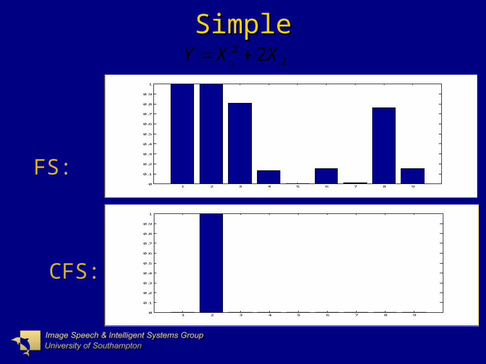
SimpleSimple

1 2 3 4 5 6 7 8 90

0.1

0.2

0.3

0.4

0.5

0.6

0.7

0.8

0.9

1

1 2 3 4 5 6 7 8 90

0.1

0.2

0.3

0.4

0.5

0.6

0.7

0.8

0.9

1

FS:

CFS:

22 21

XXY

ResultsResults

Data Set CFS FW FS FW & FS

WBC 0.0235 0.0249 0.0245 0.0249

Sonar 0.2271 0.1757 0.1629 0.1643

Votes 0.0398 0.0464 0.0650 0.0439

Pima 0.2523 0.2312 0.2492 0.2486

Ionosphere 0.0650 0.0683 0.0747 0.0653

Friedman 0.1685 0.1555 0.1420 0.1370

Simple 0.1653 0.0393 0.0283 0.0303

• 90% of data used for training, 10% for testing

• Forests of 100 trees were tested and averaged over 100 trials

• 100 trees constructed for feature evaluation in each trial

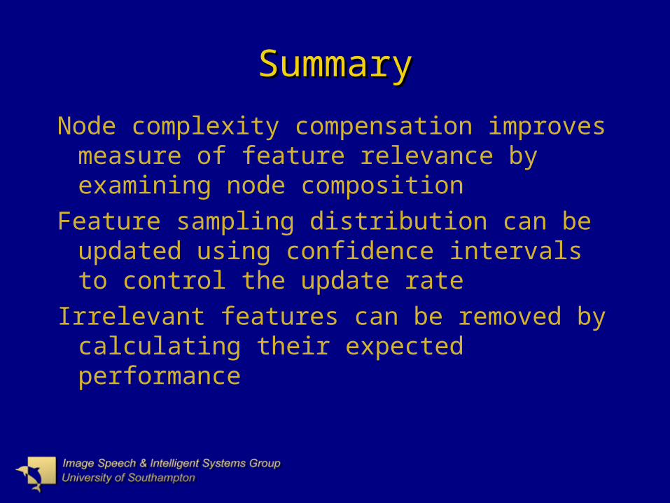
SummarySummary

Node complexity compensation improves measure of feature relevance by examining node composition

Feature sampling distribution can be updated using confidence intervals to control the update rate

Irrelevant features can be removed by calculating their expected performance