How to incorporate accident severity and vehicle …ceprofs.tamu.edu/...al._Severity_in_hotspot_identification_process.pdfMiranda-Moreno, Fu, Ukkusuri, Lord 1 Paper: 09-2824 How to

Miranda-Moreno, Fu, Ukkusuri, Lord

1

Paper: 09-2824

How to incorporate accident severity and vehicle occupancy into the hotspot identification process?

Luis F. Miranda-Moreno Assistant Professor

Department of Civil Engineering & Applied Mechanics McGill University

Montreal, Quebec H3A 2K6 Phone: (514) 398-6589 Fax: (514) 398-7361

Email: [email protected]

Liping Fu Professor

Department of Civil & Environmental Engineering University of Waterloo

Waterloo, ON, N2L 3G1 Phone: (519) 888-4567 ext 33984

Fax: (519) 725-5441 Email: [email protected]

Satish Ukkusuri

Assistant Professor Department of Civil and Environmental Engineering

Rensselaer Polytechnic Institute Phone: (518) 276-6033 Fax: (212) 995-4166 Email : [email protected]

Dominique Lord

Assistant Professor Department of Civil Engineering

Texas A&M University Phone: (519) 77843-3136

Fax. (979) 845-6481 Email: [email protected]

Paper presented at the 88th Annual Meeting of the Transportation Research Board March 23, 2009

Word count ≈ 5000 (text) + 10*250(tables and figures) ≈ 7,500


2

Abstract This paper introduces a Bayesian accident risk analysis framework that integrates both accident frequency and its expected consequences in the hotspot identification process. This Bayesian framework allows the introduction of uncertainty not only in the accident frequency/severity model parameters but also in key variables such as vehicle occupancy levels and severity weighing factors. For modeling and estimating the severity levels of each individual involved in an accident, a Bayesian multinomial model is proposed. For modeling accident frequency, we use hierarchical Poisson models. We also show how our framework can be implemented to compute alternative relative and absolute measures of total risk for hotspot identification. To illustrate the applicability of our proposed approach, a group of highway-railway crossings from Canada is used as an application environment.

1. Introduction Recognizing the deficiencies of the accident-risk estimates based on raw data, the traffic safety community has shown a continuous interest in the development and application of the risk-model based approach - which makes use of statistical methods based on probability theory. This approach consists of a systematic analysis of the input crash data in order to develop accident frequency and/or consequence models from which some ranking criteria are built (e.g., 1-3). Once statistical models have been developed from the input data, several Bayesian ranking methods or criteria proposed in the literature can be applied to identify a list of hotspots (1-8). These criteria include the posterior expectation of accident frequency, potential of accident reduction and posterior expectation of ranks. These measures usually assume that the safety status of a site can be reflected by accident frequency, and severity is usually not incorporated in the analysis or is assumed to be fixed over locations (observed and unobserved severity heterogeneities are ignored across sites). In many applications, however, accident frequency may not completely reveal the total risk level of a site and capture the potential safety benefits that some safety countermeasures could introduce. For example, in highway-railway networks, some safety measures such as speed limits have a more significant effect on train-vehicle collision severity than frequency. Although most published work on hotspot identification mainly focuses on developing separately accident frequency and consequence models, few screening studies have proposed frameworks that integrate both elements in a two-dimensional risk approach including uncertainty in the analysis (see e.g., 9-10). This approach assumes that the accident occurrence at a location is best represented by the product of accident frequency and severity. One way to incorporate accident severity in the analysis consists of calibrating statistical models that relate the accident consequences with factors such as location configuration, roadway alignment, speed limits, surface conditions, etc. (9-11). In this stage, the aim is to identify the factors that largely influence the likelihood of fatal or injury outcomes once an accident takes place. For the severity analysis, several statistical model settings have been suggested in the literature, such as the basic logistic regression, multinomial, ordered logit and mixed logit models (e.g., 11-12). Alternatively, some studies incorporate accident consequences by simply classifying accident counts by severity types (e.g., fatal and injury and other accident types), for instance see (6), (13). In this case, a statistical multivariate model setting considering the different categories is implemented (multivariate analysis). Although this approach accounts for correlation among crash counts, the expected crash consequences (for drivers and passengers) do not vary across


3

locations and vehicle occupancy levels as an important determinant of overall risk exposure is ignored. Note that vehicle occupancy has been an important part of transportation management systems and is used for evaluating high-occupancy vehicle (HOV) lanes or congestion reduction strategies (14). However, vehicle occupancy levels as a determinant of traffic risk exposure has been often ignored in the implementation and evaluation of traffic safety strategies. This paper introduces a new hierarchical Bayesian framework to integrate accident frequency, severity and vehicle occupancy levels in the hotspot identification process. The primary intention of the paper is to illustrate the potential effect of incorporating accident severity on the result of the hotspot identification process. For this purpose, we use a group of highway-railway crossings from Canada as an application environment. This paper is organized in the following way. Section 2 introduces the severity model structure and some absolute and relative measures of total risk for ranking and selecting hotspots. Section 3 presents an illustrative case study using highway-railway intersections. Section 4 summarises main conclusions and some directions for future work. 2. A Total risk based Approach In this section, the elements of our proposed Bayesian risk-based methodology are defined, including severity score, accident consequence model and hotspot identification criteria. 2.1 Severity score definition Total risk is commonly defined as the product of the accident frequency and consequences - e.g. see (10). That is,

TRi = θi × Ci, (1)

where TRi is the total risk at site i (i=1,… n sites), θi is the mean number of accidents and Ci is the expected consequence caused by an accident taking place at site i. Previous research has mainly focused on how to estimate accident frequency; our work, therefore, focuses on how to compute Ci. In addition, under a Bayes framework, both θi and Ci can be considered as random variables. Moreover, recognizing the fact that an accident could result in different types of outcomes, such as fatal, major and minor injuries, and property damages, the total consequence should, therefore, encapsulate at least the major types of outcomes. As a result, we define Ci as a severity score, integrating three components as follows: Ci 33i22i11i fff ω⋅+ω⋅+ω⋅= , (2) where, f1i, f2i and f3i are the expected number of fatal, serious and minor injuries, respectively, under an accident taking place at site i; ω1, ω2 and ω3 are estimated equivalent “monetary” costs (or pre-specified weights) per fatality, serious injury and minor injury, respectively. Three examples of these equivalent costs are given in Table 1 (e.g., see 10, 15). Note that, in the proposed integration approach, other costs, such as property damage, emergency services, and delays, are ignored - these are usually small or proportional to other injury costs.


4

The expected number of casualties of a given severity type in Equation 2, can be estimated by multiplying the expected number of passengers per vehicle (estimated motor vehicle occupancy) by the probability under which a person involved in an accident suffers that type of severity, that is, fki = pki × hi (3) where pki represents the probability that a passenger involved in a collision at site i with specific-site attributes will be injury type k (k=1,2 and 3), and hi refers to an average number of passengers involved in an accident. Since in some practical application hi may be difficult to estimate, a common nominal (h) value could be assumed to different subgroups of sites. Based on past vehicle occupancy studies and/or vehicle occupancies reported in accident records, an analyst should be able to define various occupancy weighting values for different subgroups of sites. For example, high weights could be assigned to locations with high percentage of vehicles with high levels of occupancy (14). This will allow vehicle occupancy level being considered as an important determinant of the overall crash risk exposure in roadway facilities. 2.2 Collision consequence modeling In order to estimate the total accident consequences using Equations 2 and 3, we need to estimate the probability that a passenger involved in a collision will suffer each given injury type (pki). For doing so, we introduce the use of a Bayesian severity model setting, which assumes that the outcome of a collision follows a multinomial distribution. In this model, we can incorporate information about vehicle occupancy in which each person involved in a collision has four possible severity types: fatality, severe injury, minor injury, and no injury. Note that alternatively an ordinal Bayesian model could be formulated for the injury outcomes; however, a comparative analysis is out of the scope of this paper. In addition, a random effect at the site level could be introduced in our model to account for intra-site correlation since accidents coming from the same site can be nested. However, we show only the basic model formulation for illustrative purpose. In order to model the severity of an accident, we assume that an accident could lead to K possible injury outcomes, denoted by r = }{ k1 r,...,r , where k stands for injury type, k=(1,…,K). Suppose, also, that there are h persons involved in an accident and for each person involved in an accident he/she could suffer from a specific injury outcome k with probability pk. Then, by assuming that r follows a multinomial distribution, we can model an accident outcome as, r | p ~ Multinomial(h, p), (4) where:

h = number of persons involved in an accident (note that r1,…,rK are nonnegative integers),

p = vector of probabilities p=(p1,…,pK), pk being the probability that a person involved in an accident has an injury of type k (pk > 0).

Then, the probability that an involved person will have a type k injury can be estimated using the following logit regression:


5

pik = ∑

=

== K

1kik

ik

)exp(

)exp()kpassangera(obPr

ϕ

ϕ (5)

where, ϕik is a measure representing the propensity for a person involved in an accident with specific traits i to experience severity type k. Here, ϕik is expressed as a linear function of site characteristics, environment, and individual attributes: mimki1k1k0ik z...z γγγϕ +++= (6) where, zi =(z1i,…, zmi) represents site, vehicle, or other characteristic (e.g., speed limits, location characteristics where accident took place, vehicle type, etc.) and γk ),...,( 0 mkk γγ= is a vector of regression parameters. In our model, a Gaussian non-informative prior is assumed on these parameters. Once the proposed model is calibrated with empirical data, we can estimate, for instance, the expected number of fatalities, (serious/minor) injuries, and non-injuries, by Equation 3, i.e., fki = E(rk) = pki × hi. After computing the expected number of casualties by type, we can estimate the total severity score Ci, according to Equation 2, where the f-values vary across locations, depending on attributes such as posted road speeds, maximum train speeds and levels of occupancy, among others. Furthermore, ω1, ω2, and ω3 are usually provided by insurance or governmental agencies. In our approach, these weights can be assumed to be fixed or to follow a known prior distribution with parameters fixed according to different cost estimates such as those reported in Table 1. Other components may also be included in the cost per accident such as costs for property damage, delays and emergency services. Even so, there is often not enough information to incorporate these extra costs. Also, these extra costs are usually smaller than the cost of fatalities and injuries. This modeling setting is based on the idea that there are different collision configurations across sites. Thus, there are variations in the injury type probabilities that can be explained by site-specific factors, such as roadway features (posted road speed, urban/rural site, surface width, etc.) as well as environmental conditions, passenger and vehicle characteristics. Obviously, the set of factors that can be included depends on the data availability. Moreover, there are also many unobservable factors that affect the injury levels (e.g. two passengers with the same observable characteristics having a collision do not necessarily have the same injury level.

2.3. Ranking criteria based on absolute and relative total risk Once the severity score is determined, a hotspot strategy based on the posterior distribution of the total risk (TRi), can be specified as follows: )data|cTRPr(υ Ti

TRi >= ≥ δ0 (7)


6

where cT is a standard value established by decision-makers and δ0 is a threshold value or confidence level varying between 0 an 1. For the definition of δ0, we use the Bayesian testing methods introduced in a previous work by (16). The decision as to whether or not a site should be considered a hotspot could also be made on the basis of its relative rank as compared to other sites under a given safety measure. The rank of a site i under the total risk (TRi) is defined as follows: ∑ =

≥=n

1j jii)TR( )TRTR(Ir , (8)

where I(condition) is an indicator function with the value 1 if the condition is met and 0 otherwise. The index TR in r stands for the relative comparison under total risk. Given that the safety measure TRi is a random variable, the resulting rank

i)TR(r , is also a random variable with its posterior distribution depending on the relative comparison of TRi with respect to the others. Hotspots can be then identified on the basis of the ranks of the sites by computing the following posterior probability: r

iυ = )data|qrPr( i)TR( > , then if riυ > δ1, site i is a hotspot (9)

where q is a standard or upper limit rank specified by the decision-makers. For instance, we can define q as a certain proportion of n, that is, q = τ×n, where τ is a percentage, e.g., 70%, 80%, etc. This hotspot selection strategy can be used when the interest focuses on the identification of sites with ranks greater than a certain percentile value. Once iυ is computed under equation 9, the optimal cutoff value δ1 can be determined using any of the multiple testing procedures introduced by (16). Note also that inference based on posterior of ranks can be done according to any of the safety measures previously defined.

3. Case study To illustrate our proposed approach, a sample of highway-railway intersections in Canada is considered as an application environment. For this case study, we consider a group of public crossings in Canada with automatic gates as the main warning device; these comprise approximately 1,773 crossings. Automatic gates provide an additional control level and are usually in conjunction with flashing lights. The gate arms are usually reflectorized and fully cover the approaching roadway to prevent motor vehicles from circumventing the gates, which are coordinated with the flashing lights (Figure 1). All crossings use 2-quadrant gates with dual gate arms, which block motor vehicles in each direction. Once a crossing of this type is identified as a hotspot, it could be further upgraded with new countermeasures such as 4-quadrant gates or median separation, which can prevent vehicles from driving around lowered gates, or grade separation. The main characteristics of this dataset are summarized in Table 2. From this table, we can observe that this dataset is characterized by a high proportion of zero accidents (and low mean), which is a common characteristic in accident data. Prior to the model calibration, an exploratory data analysis is carried out. This preliminary analysis seeks to identify high linear correlation


7

among covariates and to detect observations with extreme values or missing information. The correlation among crossings attributes was moderate and surface width is not included in the analysis because this information is missing for many crossings.

3.1 Frequency model calibration For illustration purposes, we concentrate on the application of two hierarchical Bayes models: the Poisson/Gamma with a multiplicative error term - exp(εi)∼Gamma(φ,φ) - and Poisson/Lognormal model with an additive error, εi∼Normal(0,σ2). As described in (17), the parameters “a” and “b” of the hyper-prior distribution assumed on φ or σ-2 (φ∼Gamma(a,b) and σ-2~Gamma(a,b)) might be first specified. For the hierarchical Poisson/Gamma model, we could assume non-informative priors with very small values for these parameters, e.g., a=b=0.01 or a=b=0.001. However, in this study, we take a more reasonable approach by taking advantage of the dispersion parameter estimate (φ̂ ) obtained by maximizing the NB marginal likelihood (16). For instance, for this dataset, we first calibrated the NB model, which yielded a dispersion parameter of φ̂ =0.64. Based on the fact that the expectation of the Gamma distribution assumed for φ is a/b and by fixing a=1, we can then assume that E( )b/1()b| =φ = 0.64, from which b=1.56. In this case study, vague hyper-priors are assumed for σ-2 with both parameters a=b=0.01 or a=b=0.001 for the hierarchical Poisson/Lognormal model.

Once the hyper-parameters are fixed, posterior distributions are sampled using the statistical software WinBUGS. In this study, 6000 simulation iterations were carried out for each parameter of interest, using the first 2000 samples as burn-in iterations. In order to select the crossing attributes to be included in the final model, we first obtained the posterior expected values of all the regression coefficients, along with their standard deviations and 95% confidence intervals. From those, we only selected the attributes whose regression coefficients did not contain 0 in the 95% confidence intervals (i.e., regression parameters significantly different from zero at the 95% confidence level). These crossing attributes are:

1) Road type represented as a binary variable (road type=1 for arterials or collectors, and 0 otherwise),

2) Posted road speed (km/h), and 3) Traffic exposure (Ei ) computed as a function of daily road vehicle traffic (AADTi) and

number of daily trains (ti), i.e., Ei = AADTi × ti. The posterior summary of the covariate coefficients ( β ) along with the dispersion parameters φ and σ2 were computed for both the Poisson/Gamma and Poisson/Lognormal models, respectively. The results are presented in Table 3. The posterior mean of the regression coefficients is positive, except 0β , making sense from a safety point of view and confirming the results obtained in our previous work (7, 18). In addition, from the DIC results presented in the same table, we can see that a better fit to the data was obtained when applying the Poisson/Gamma model. As expected, the DIC value computed with the Poisson/Gamma model with semi-informative prior on (use of the ML estimate of the NB model,φ̂ ) is smaller than the one obtained with the Poisson/Lognormal model with vague hyper-prior on the dispersion


8

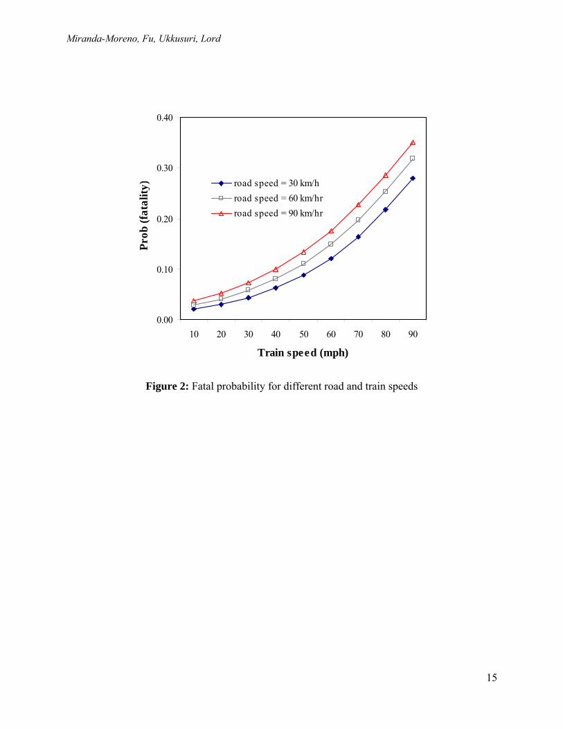
parameter. As stated earlier, a sensitivity analysis on alternative prior specifications is always recommended in order to identify the best alternative model. Given the large sample (n=1773) used in this exercise, the model outcome is not very sensitive to the prior assumptions. Based on the results of this analysis, it was decided to use Poisson/Gamma in our subsequent analysis. 3.2 Severity model calibration To calibrate the parameters of the proposed severity model, the collision database for the period from 1997-2004 was utilized. This includes a total of 941 highway-railway grade crossing collisions as summarized in Table 4. Alternative specifications were attempted for the function ϕik, from which it was found that both maximum train speed and posted road speed are the main salient factors influencing significantly collision severity at a crossing, that is, ϕik

i2k2i1k1k0 zγzγγ ⋅+⋅+= , where, z1i and z2i are maximum train and road posted speeds. The calibration results are shown in Table 5, where the parameters for severity type 1 (fatality) are not shown, as severity type 1 is set as base type with parameters equal to zero. The selection of this model was supported on the Deviance information criterion (DIC). Figure 2 shows how p1i varies as a function of maximum train and posted road speeds. From this figure, we can see that the outcomes of a highway-railway crossing collision are very sensitive to maximum train speeds. 3.3 Hotspot identification using total risk Based on the same group of highway-railway crossings with gates as a main warning device (n=1773 intersections) and the hierarchical Poisson/Gamma model defined above, the υ-values were computed for the hotspot identification. For doing so, a Bayesian approach was implemented using a MCMC framework. One of the advantages of this framework is that different sources of information and uncertainty can be incorporated into the analysis. Graphically, the multiple sources of information (parameters) in this decision process are illustrated in Figure 3. Note that in our framework, not only the model parameters (β, η, θi) are assumed random, but also the uncertainty with Ci can be introduced by defining a prior distributions in different model parameters, including ω, hi and γ. In this demonstrative example, a value of cT =1 is defined according to the weights defined in Table 1, which is equivalent to the cost of a serious injury. In addition, we use an average level of occupancy (Oi) equal to 1.29 (which corresponds to the average vehicle occupancy of the recorded collisions involved in this analysis). Once the different model parameters are fixed, MCMC algorithms can be employed for the computation of υ-values. Finally, a Bayesian testing approach is used for the definition of δ0 (16). Hence, by fixing cT =1 and controlling the false-discovery rate (FDR) at 10% (αD=10%), the optimal thresholds and hotspot list sizes are presented in Table 6. Also, using a Bayesian test with weights for κ0 = 3 and κ1 = 1, the threshold values and the hotspot list sizes are given in the same table. The codes for computing the model parameters and υ-values are provided in (18). For estimating the parameters of the Bayesian Poisson and multinomial logit models and, the posterior υ-values, the software package WinBugs was used. Written codes can be seen in (18) and they may be also available upon request.


9

As we can see in both Table 6 and Figure 4, the hotspot list size is very sensitive to the weight assigned to the fatalities (ω1). For instance, for a given value of cT and a specific control level (αD), the hotspot list size increases in a nonlinear way as ω1 increases. Note that the designation of a weight (or monetary value) to a human life may be controversial. However, in the hotspot identification activity, this helps to target those locations where, not only the accident frequency will be high, but also the consequences. For instance, in the case of highway-railway crossings, intersections with high maximum train and posted road speeds will be pushed up in the ranking, since the accident severity at these sites will be higher. 3.4 Practical application of the proposed methodology For practitioners, the implementation of the modeling framework introduced above may not be straight forward. This demands some advanced statistical and computational knowledge which could significantly hinder its application for addressing practical problems. Recognizing this issue, a web-based decision support tool called GradeX has been developed (for details, see www.gradex.ca/). This tool makes accessible to practitioners some state-of-the-art risk-based methodologies for hotpot identification such as the one introduced in this paper. GradeX is currently used by Transport Canada and all of its regional offices to identify grade crossing hotspots and analyze alternative countermeasures for safety improvements. It integrates a rich set of accident prediction models and risk assessment methodologies, including the multinomial logit model presented in this paper. GradeX also offers state-of-the-art methodologies for countermeasure effectiveness analysis. It provides users with a convenient interface to define a set of crossings to be investigated, which facilitates analysis of crossings located within any geographical area, such as region, municipality and corridor (for details see, (19)). 4. Conclusions and future work One of the common approaches to hotspot identification is first to rank candidate sites based on a safety measure, and then select the top sites according to a critical value. However, little research has been conducted in literature on the issue of how to incorporate heterogeneities across locations in the severity and occupancy levels at the hotspot identification stage. In this research, we proposed a systematic full Bayesian framework for estimating the total risk of a given site as the product of accident frequency and its expected consequences. This Bayesian framework allows the introduction of severity uncertainty not only in the model parameters but also in key factors such as vehicle occupancy levels and severity weighing factors. The proposed framework also allows identifying hotspots under relative or absolute measures of total risks, controlling appropriate global error rates, such as a false positive error rate. The applicability of our framework is illustrated using an accident dataset from Canadian highway-railway crossings with automatic gates. To estimate the total accident consequences, the probability that a passenger involved in a collision is fatally or seriously injured is estimated using a Bayesian multinomial model. In this model, we can incorporate information about vehicle occupancy in which each person involved in a collision has several possible severity outcomes, such as fatality, severe/ minor injury, and no injury. In addition, hierarchical Poisson models with additive and multiplicative model errors are used for modeling accident frequency. For this particular case, the Poisson/Gamma model fits better the observed data than the Poisson/Lognormal. Finally, multiple Bayesian tests are implemented to control the proportion of false positives in the hotspot list


10

Considering the number of persons involved in an accident in concert with number of crashes is expected to improve the effectiveness of allocating resources to various safety programs. It is recognized, however, that the inclusion of vehicle occupancy in road safety analysis may represent some challenges in practical applications – obtaining occupancy data for each location involved in the analysis can be an expensive and time consuming task. However, in safety studies in which detailed occupancy information is not available, sites can be classified according to the proportion of high-occupancy vehicles, such as transit and school buses. Alternatively, as shown in this work, average vehicle occupancy levels can be approximately determined for various subgroups of locations based on the vehicle occupancies reported in accident data. The premise is that, with the proposed model, locations with a higher average vehicle occupancy would be given a higher chance to be included in the hotspot list. As part of our current research effort, a safety measure that estimates the “anticipated” cost-benefit ratio is being developed. Since a hotspot selection strategy has the aim to direct the safety improvement efforts towards sites where maximum cost-effectiveness can be achieved, it would be of great value if the process could also take into account both the costs and safety benefits of possible remedy projects that could be introduced to the sites under consideration (4). Hierarchical ordered models are to be developed and integrated in our risk-based framework. The comparative performance of relative versus absolute measures of risk is also part of our future research. It is also necessary to explore the use of new technologies to improve existing methods for occupancy data collection. The evolution of vehicle occupancy and its implications on road safety also deserves further investigation.


11

References 1. Schluter, P.J., J.J. Deely and A.J. Nicholson. Ranking and Selecting Motor Vehicle

Accident Sites by Using a Hierarchical Bayesian Model. The Statistician, 46 (3), 1997, pp. 293-316.

2. Heydecker, B.G., and J. Wu. Identification of Sites for Accident Remedial Work by

Bayesian Statistical Methods: An Example of Uncertain Inference. Advances in Engineering Software, 32, 2001, pp. 859-869.

3. Hauer, E., J. Kononov, B.K. Allery and M.S. Griffith. Screening the Road Network for

Sites with Promise. Transportation Research Record: Journal of the Transportation Research Board, No. 1784, 2004, pp. 27-31.

4. Hauer, E., and B.N. Persaud. How to Estimate the Safety of Rail-highway Grade

Crossings and the Safety Effects of Warning Devices. Transportation Research Record: Journal of the Transportation Research Board, No. 1114, 1987, pp. 131-140.

5. Persaud, B., C. Lyon, and T. Nguyen. Empirical Bayes Procedure for Ranking Sites for

Safety Investigation by Potential for Safety Improvement. Transportation Research Record: Journal of the Transportation Research Board, No. 1665, 1999, pp. 7-12.

6. Miaou, S.P., and J.J. Song. Bayesian Ranking of Sites for Engineering Safety

Improvement: Decision Parameter, Treatability Concept, Statistical Criterion and Spatial Dependence. Accident Analysis and Prevention, 37, 2005, pp. 699-720.

7. Miranda-Moreno, L.F., L. Fu, F. Saccomanno and A. Labbe. Alternative Risk Models for

Ranking Locations for Safety Improvement. Transportation Research Record: Journal of the Transportation Research Board, No. 1908, 2005, pp. 1-8.

8. Cheng, W., and S.P. Washington. Experimental Evaluation of Hotspot Identification

Methods. Accident Analysis and Prevention 37, 2005, pp. 870–881. 9. Nassar, S., F.F. Saccomanno and J.H. Shortreed. Disaggregate Analysis of Road

Accident Severities. International Journal of Impact Engineering 15(6), 1994, pp. 815-826.

10. Saccomanno, F.F., L. Fu, and L.F. Miranda-Moreno. Risk-Based Model for Identifying

Highway-Rail Grade Crossing Blackspots. Transportation Research Record: Journal of the Transportation Research Board, No. 1862, 2004, pp. 127-135.

11. Milton, J.C., V.N. Shankar, L. Fred and F.L. Mannering. Highway Accident Severities

and the Mixed Logit Model: An Exploratory Empirical Analysis. Accident Analysis and Prevention 40, 2008, pp. 260-266.


12

12. Eluru, N., C.R. Bhat, and D.A. Hensher. A Mixed Generalized Ordered Response Model for Examining Pedestrian and Bicyclist Injury Severity Level in Traffic Crashes. Accident Analysis and Prevention, 40(3), 2008, pp. 1033-1054.

13. Park, E.S., and D. Lord. Multivariate Poisson-Lognormal Models for Jointly Modeling

Crash Frequency by Severity. Transportation Research Record: Journal of the Transportation Research Board, No. 2019, 2007, pp. 1-6.

14. Levine, N. and M. Wachs. Factors Affecting Vehicle Occupancy Measurement. Transportation Research A, 32(3), 1998, pp. 215-229.

15. Zaloshnja, E., T. Miller, F. Council, and B. Persaud. Crash Cost in the United States by Crash Geometry. Accident Analysis and Prevention, 38, 2006, pp. 644-651.

16. Miranda-Moreno, L.F., A. Labbe, and L. Fu. (2007), Multiple Bayesian Testing

Procedures for Selecting Hazardous Sites. Accident Analysis and Prevention, 39(6), 2007, pp. 1192-1201.

17. Lord, D., and L.F. Miranda-Moreno. Effects of Low Sample Mean Values and Small

Sample Sizes on the Dispersion Parameter Estimation of Poisson-Gamma Models for Modeling Motor Vehicle Crashes: A Bayesian Perspective. Safety Science 46(5), 2008, pp. 751-770.

18. Miranda-Moreno, L.F., (2006), Statistical Models and Methods for Identifying Hazardous

Locations for Safety Improvements, PhD thesis, University of Waterloo.

19. Fu, L., F. Saccomanno, L. Miranda-Moreno, Y-J Park and J. Chen. GradeX - A Decision Support Tool for Hotspot Identification and Countermeasure Analysis of Highway-Railway Grade Crossings. CD-ROM. Transportation Research Board of the National Academies, Washington, D.C., 2007.


13

Figures

Figure 1: A standard level crossing with gates

Figure 2: Fatal probability for different road and train speeds

Figure 3: Modeling framework for computing total risk

Figure 4: List size sensitivity to the fatal weights

Tables

Table 1: Direct severity costs per person and weights assumed in this analysis

Table 2: Variables and statistics of the crossing dataset with gates

Table 3: Posterior estimates of the model parameters

Table 4: Summary of collisions by severity

Table 5: Calibration results of the consequence models

Table 6: Threshold values and hotspot list size under total risk


14

Figure 1: A standard level crossing with gates


15

0.00

0.10

0.20

0.30

0.40

10 20 30 40 50 60 70 80 90

Train speed (mph)

Prob

(fat

ality

) road speed = 30 km/hroad speed = 60 km/hrroad speed = 90 km/hr

Figure 2: Fatal probability for different road and train speeds


16

Figure 3: Modeling framework for computing total risk


17

0.0

10.0

20.0

30.0

40.0

0 50 100 150 200 250

Hotspot list size

FDR

-con

trol

leve

l

ω1 = 41

ω1 = 30

ω1 = 15

Figure 4: List size sensitivity to the fatal weights


18

Table 1: Direct severity costs per person and weights assumed in this analysis

Source Cost estimates (US dollars) Weightsd

Fatality, Serous injury Minor injury ω1 ω2 ω3

1 2,710,000a 65,590 30,000 41 1.0 0.5

2 2,000,000b 65,590 30,000 30 1.0 0.5

3 1,000,000c 65,590 30,000 15 1.0 05 a Cost employed by Saccomanno et al (2004). b Cost reported by Zaloshnja et al (2006).

c Cost designated for US agencies, e.g. National Safety Council, www.nsc.org/resources/issues/estcost.aspx. d The weights are relative to the serious injury cost. The serious and minor injury costs are the same as the

ones proposed by Saccomanno et al (2004). The weights are obtained by dividing each cost by the serious

injury cost.


19

Table 2: Variables and statistics of the crossing dataset with gates Variable Unit Average/% St. dev. Max. Min.

Road class Arterial/collector =1, 0 others 44.0%

Track number Number 1.9 0.9 8.0 1.0

Track angle Degree 72.5 18.4 120.0 0.0

Train maximum speed Mph 56.4 24.3 100.0 5.0

Road posted speed Km/hr 59.3 16.1 100.0 15.0

Number of daily trains (F1)

Trains/day 22.3 22.8 338.0 1.0

AADT (F2) Vehicles/day 4162.7 6041.7 48000.0 10.0

Traffic exposure Ln(F1×F2) 10.1 1.7 15.9 3.9

Whistle prohibition if prohibited =1, 0 otherwise 35.2%

Surface width Ft 11.4 7.2 75.0 0.0

Number of collisions Number (five-year period, 1997-2001) 0.12 0.4 4.0 0.0


20

Table 3: Posterior estimates of the model parameters

Hierarchical model Attributes Posterior

mean Std. Dev.

MC error

Conf. Interval (2.50%-97.50%)

Poisson/Gamma a=1.56

Intercept β0 -6.429 0.717 0.076 (-7.764, -4.955)

Road type β1 0.499 0.164 0.007 (0.171, 0.815)

Posted road speed β2 0.011 0.005 0.000 (0.001, 0.021)

Traffic exposure β3 0.323 0.054 0.005 (0.214, 0.429)

φ 0.691 0.237 0.025 (0.381, 1.332)

DIC = 1191.25

Poisson/Lognormal a=0.001 b=0.001

Intercept β0 -7.041 0.72 0.08 (-8.316, -5.657)

Road type β1 0.506 0.17 0.01 (0.167, 0.842)

Posted road speed β2 0.011 0.01 0.00 (0.001, 0.022)

Traffic exposure β3 0.327 0.05 0.00 (0.228, 0.421)

σ 1.016 0.14 0.01 (0.706, 1.296)

DIC = 1220.40


21

Table 4: Summary of collisions by severity

Variables Total Average

(#/Collision) Max. Min.

No. of Accidents 941 --- --- ---

No. of occupants (Persons involved) 1217 1.29 21 1.0

Fatalities 137 0.15 3.0 0.0

Serious injuries 189 0.20 3.0 0.0

Minor injuries 241 0.26 7.0 0.0


22

Table 5: Calibration results of the consequence models

Severity type

Variable Coefficient Posterior mean

Std. Dev. MC error

Conf. Interval (2.50%-97.50%)

Fatal (Base type) γ11=γ21= γ11 =0

Major injury

Intercept γ02 1.462 0.305 0.025 (0.833, 2.026) Train speed γ12 -0.021 0.005 0.000 (-0.030, -0.010)

Minor injury

Intercept γ03 2.072 0.306 0.026 (1.412, 2.698) Train speed γ13 -0.028 0.005 0.000 (-0.038, -0.018)

No injury Intercept γ04 4.459 0.319 0.028 (3.832, 5.134) Train speed γ14 -0.042 0.004 0.000 (-0.051, -0.033) Road speed γ24 -0.014 0.003 0.000 (-0.020, -0.008)


23

Table 6: Threshold values and hotspot list size under total risk

Severity weights

FDR test (αD=10%)

Bayesian test with weights (κ0=3 and κ1=1)

Threshold (δ0) # of hotspots Threshold (δ0) # of hotspots

ω1=15, ω2 =1, ω3=0.5 0.83 32 0.75 52

ω1=30, ω2=1, ω3=0.5 0.80 66 0.75 77

ω1=41, ω3=1, ω3=0.5 0.76 105 0.75 111

Documents

How to incorporate accident severity and vehicle …ceprofs.tamu.edu/...al._Severity_in_hotspot_identification_process.pdfMiranda-Moreno, Fu, Ukkusuri, Lord 1 Paper: 09-2824 How to