Embed Size (px)
Citation preview

How Infrastructure Investments Support the U.S. Economy: Employment, Productivity and Growth
James HeintzAssociate Research Professor& Associate Director Robert PollinProfessor of Economics & Co-Director Heidi Garrett-PeltierResearch Assistant
Political Economy Research Institute
JANUARY 2009


INFRASTRUCTURE INVESTMENTS AND THE U.S. ECONOMY
Summary of Main Findings
The United States system of civilian public infrastructure has deteriorated badly over the past generation. The breaching of New Orleans’ water levees in 2005 in the wake of Hurricane Katrina and the collapse of the I-35W bridge in Minneapolis in 2007 offered tragic testimony to this long-acknowledged but still neglected reality.
After this generation of neglect, the project of rebuilding our infrastructure now needs to be embraced as a first-tier economic policy priority, and not simply to prevent repetitions of the disasters in New Orleans and Minneapolis. The more general point is that infrastructure investments are essential for the functioning of the U.S. economy. According to the U.S. Bureau of Economic Analysis, total public assets, excluding defense, were valued at $8.2 trillion in 2007. This represents approximately 50 percent of the stock of all non-residential private assets—a formidable asset base which underpins the national economy.
Core economic infrastructure—in the areas of energy, transportation, and water and sewerage—is particularly important in maintaining economic performance. However, the rate of public investment in these core areas began falling in the 1970s and has not returned to its previous levels since then. As an average since 1980, the growth of infrastructure investment has lagged behind overall economic growth. The result has been a worsening infrastructure deficit and mounting investment needs.
With the rapid deterioration of economic conditions in recent months and rising unemployment, public investment is back on the policy agenda—as a job-creation program linked to the need to revitalize the nation’s crumbling infrastructure. In November 2008, President-elect Obama announced his intention of creating 2.5 million jobs by introducing a large-scale public investment program during his first two years in office. Since this initial announcement, the proposed size of the stimulus package and the job-creation targets have varied. Nevertheless, public investment remains at the center of thinking about the ‘new New Deal’—the set of policies that are needed to address the ongoing crisis.
In this report, we examine the employment impacts of an expanded infrastructure investment program and what it would take to create millions of jobs. We develop specific policy scenarios based on an assessment of the nation’s infrastructure needs in four core areas—transportation, energy, water systems, and public school buildings—and estimate the employment that would be created if the policies were implemented, with a specific focus on manufacturing employment. We also examine what the long-run impacts of such a program would be in terms of productivity and overall economic growth. Finally, we offer some brief observations on both U.S. competitiveness and environmental sustainability that emerge directly from our main findings.

H O W I N F R A S T R U C T U R E I N V E S T M E N T S S U P P O R T T H E U . S . E C O N O M Y ■ P A G E 2
Some of the key findings include the following:
Assessing U.S. Infrastructure Needs
Estimating assessed needs. Based on assessments from a range of government agencies and private studies, we estimate a “baseline” infrastructure investment level that would adequately meet the economy’s assessed needs over the next five years. We also present a “high-end” assessment that would accelerate the project of meeting our long-term infrastructure needs.
Baseline assessment. Our baseline estimate of infrastructure investment needs amount to $87 billion per year, of which about $54 billion would come from the public and $33 billion would be private investment. This amounts to a $275 billion investment project over the next five years.
High-end assessment. Our high-end estimate is $148 billion per year, of which $93 billion would need to come from the public sector, and $55 billion from the private sector.
Infrastructure Investments and Economic Growth Rise and Fall Together
1950-79: Public infrastructure investment and economic growth rise together. Between 1950 – 79, public investments in core areas—transportation, water manage-ment, and electricity transmission—grew at an average annual rate of 4.0 percent. Overall economic growth (GDP) averaged 4.1 percent per year over that same period.
1980-2007: Public infrastructure investment and economic growth fall together. Between 1980 – 2007, public investment growth slows dramatically, to an average 2.3 percent. GDP growth also falls in this more recent period, to a 2.9 percent average annual rate.
Faster public investment growth produces faster overall growth. The change in the public investment growth rate is a significant contributor to GDP growth. For the year 2007, the impact due to both our baseline and high-end scenarios from an increase in public infrastructure investments only (holding aside private infrastructure investments) would be as follows:
o Baseline scenario: The $54 billion baseline increase in public infrastructure investment would yield an annual GDP increase of about $46 billion. This would provide an annual productivity dividend of about $150 for every U.S. resident. o High-end scenario: The $93 billion high-end increase in public infrastructure investment would yield an annual GDP increase of about $77 billion. This is a productivity dividend of about $260 per year for every U.S. resident.

H O W I N F R A S T R U C T U R E I N V E S T M E N T S S U P P O R T T H E U . S . E C O N O M Y ■ P A G E 3
Infrastructure Investments and Job Creation
Three types of job creation: direct, indirect, and induced effects. Direct job creation refers to the jobs directly involved in constructing the new infrastructure projects. Indirect job creation refers to the jobs generated when supplies are purchased for the infrastructure projects. Induced jobs are created when the overall level of spending in the economy rises, due to workers newly receiving incomes when they are hired to build the infrastructure projects, and to produce supplies for the project.
Infrastructure investments as job-creation tool. All forms of spending will produce jobs. But infrastructure investment is a highly effective engine of job creation. Thus, infrastructure investment spending will create about 18,000 total jobs for every $1 billion in new investment spending, including direct, indirect, and induced jobs. By contrast, a rise in household spending levels generated by a tax cut will create, at most, about 14,000 total jobs per $1 billion in spending, 22 percent less than infrastructure investments.
Overall Job Creation Based on U.S. Needs Assessments
Job creation through baseline program. Infrastructure investments of $87 billion per year to meet baseline needs will generate about 1.6 million total new jobs within the U.S., including direct, indirect and induced jobs.
Job creation through high-end program. Investments of about $148 billion per year to accelerate the rebuilding of the U.S. infrastructure will generate about 2.6 million new jobs, including direct, indirect, and induced jobs.
Job Creation by sector o Construction. The highest proportion of new jobs will be in construc-tion. For the baseline scenario, about 641,000 new construction jobs will be generated. The high-end investment scenario will generate about 1 million new construction jobs. Overall, about 40 percent of all new job creation through either investment program—including direct, indirect, and induced jobs—will be in construction. The construction sector has been severely hit by the recession, with unemployment in the industry rising from 9.4 to 15.3 percent between December 2007 and 2008. o Manufacturing. About 146,000 new manufacturing jobs will result through the baseline investment scenario, and the high-end investment scenario will generate about 252,000 new jobs. About 10 percent of the overall new job creation will be in manufacturing. Manufacturing has also been badly hit by the recession, with unemployment in the industry rising from 4.6 to 8.3 percent between December 2007 and 2008.

H O W I N F R A S T R U C T U R E I N V E S T M E N T S S U P P O R T T H E U . S . E C O N O M Y ■ P A G E 4
Job Creation and December 2008 Unemployment o Baseline program. If 1.6 million new jobs were added to the December 2008 labor market, that would reduce unemployment from its actual rate of 7.2 percent to 6.2 percent. o High-end program. If 2.6 million new jobs were added to the December 2008 labor market, that would reduce unemployment further, to 5.5 percent.
U.S. Jobs and Imports
Domestic supplies as major source of job creation. The main reason infrastructure investments create more jobs than an increase in household consumption is that the share of spending done within the U.S, as opposed to the purchase of imports, is significantly higher with infrastructure investments.
Domestic spending and imports in manufacturing. o The manufacturing sector will account for about 10 percent of the total
spending resulting from infrastructure investments, corresponding to the 10 percent share of employment increases.
o With the manufacturing sector, imports represent a significantly higher share of total spending tied to infrastructure investments. Import purchases account for between 12 – 22 percent of manufacturing supplies among the four key areas of energy, transportation, school buildings, and water management infrastructure investments.
o Raising domestic supplies up to 100 percent of total supplies would produce a total of 77,000 additional domestic jobs resulting from all infrastructure investment spending, an increase of 4 percent. But manufacturing jobs, by themselves, would account for 69,000 of the total 77,000 increase in jobs. The increase in domestic job creation within the manufacturing sector resulting from raising domestic supply purchases to 100 percent of total purchases would represent a 33 percent increase in manufacturing job creation.
Infrastructure Investments, Competitiveness, and Environmental Sustainability
Competiveness. Public investment improves private sector productivity. The impact is proportionally larger for the manufacturing sector than for the private sector as a whole. Improving the U.S. infrastructure in all four main areas—transportation systems, public school buildings, water management, and energy transmission—will improve U.S. competitiveness by contributing toward a lower-cost environment than would be possible under our aging current stock of infrastructure.
Environmental sustainability. Not all categories of public investments are aimed at producing direct environmental benefits, but some are. These would include

H O W I N F R A S T R U C T U R E I N V E S T M E N T S S U P P O R T T H E U . S . E C O N O M Y ■ P A G E 5
public transportation, freight rail, and smart grid electrical transmission system that can more efficiently transport electricity from renewable energy sources. At the same time, all public infrastructure projects promote a clean-energy economy by raising the efficiency of production, and thereby lowering the overall demand for energy for a given level of production.

H O W I N F R A S T R U C T U R E I N V E S T M E N T S S U P P O R T T H E U . S . E C O N O M Y ■ P A G E 6
I. OVERVIEW OF PUBLIC INFRASTRUCTURE INVESTMENT IN THE U.S.
The primary focus of this report is the number of jobs that would be created by improving the country’s infrastructure. However, we acknowledge at the outset that increasing domestic spending in any sector or project within the economy will produce an increase in jobs. But we focus on infrastructure investments for two reasons: First, investments in infrastructure are a relatively effective means of creating jobs. As we will see, the number of jobs generated for a given level of spending is high. But in addition, a program of accelerated investment in infrastructure would generate far greater benefits for the American population than would be reflected in the job numbers alone. Investments in infrastructure provide an indispensible resource for the U.S. economy. This includes the roads, highways, public transportation systems, accessible water supplies, water levee systems, electrical transmission systems, and school buildings which make fundamental contributions to the economy’s long-term productivity. Many of these investment areas—such as public transportation, freight rail, and enhanced smart grid electrical transmission systems—will also play central roles in building a clean energy economy in the U.S.
Most of these assets are public and the government plays a pivotal role in supplying the infrastructure needs of the nation. But not all infrastructure investments in the U.S. are provided by the government. Railroads, electric utilities, many airports, and gas companies represent the private side of infrastructure provision, although often with the aid of the public sector. It is this combination of public and private investments that maintains and improves the country’s core infrastructure. Nevertheless, the importance of public assets for the efficient functioning of the economy often is under-recognized. Therefore, we present a brief overview of public investment in the U.S. economy as a backdrop to our analysis of infrastructure needs, employment impacts, and policy options.
In 2007, the U.S. Bureau of Economic Analysis (Department of Commerce) valued the stock of all public non-defense fixed assets at approximately $8.2 trillion. It is useful to compare this with the estimated total value of all private non-residential fixed assets—$15.5 trillion. That is, the stock of non-military public assets amounts to over 50 percent of the stock of all non-residential private assets.
Despite this critical stock of public assets, rates of public investment have fallen substantially since peaking in the mid- and late 1960s. Figure 1.1 shows the rate of net public investment from 1950 to the present, measured as the rate of change of the non-defense public capital stock.1 As the figure shows, the rate of public investment—i.e. the growth rate of public assets—rose through the 1950s, peaking in 1965 at 5.5 percent per year. The growth of
1 We measure net public investment as additions to the total stock of public assets, adjusted for changes in the current price of public assets. To adjust for price variations across years, we calculated implicit price indices from the Bureau of Economic Analysis time series data on current cost public fixed capital stock and quantity indices for public capital. Using these indices, the values of the public capital stock were converted into constant 2000 dollars. The rate of net public investment is simply the growth rate of the relevant category of real fixed capital stock in the public sector.

H O W I N F R A S T R U C T U R E I N V E S T M E N T S S U P P O R T T H E U . S . E C O N O M Y ■ P A G E 7
public asset investments began to decline significantly in the 1970s. Nevertheless, for the 30-year period 1950-79, the growth of public investment averaged 4.0 percent per year. By contrast, from 1980 – 2007, the public investment grew at an average rate of only 2.3 percent per year. As the figure shows, the rate of investment growth remained fairly stable from the late 1980s onward, but at this relatively low level.
1
2
3
4
5
6
50 55 60 65 70 75 80 85 90 95 00 05
Figure 1.1Average Real Growth of U.S. Public Investment, 1950-2007
Perc
enta
ge a
nnua
l gro
wth
rat
e
Note: Figures are in real, inflation-adjusted dollars.Source: U.S. Department of Commerce, Bureau of Economic Analysis
4.0% average growth1950-79
2.3% average growth,1980-2007
Figure 1.2 provides further perspective on the growth trajectory of U.S. public investment, by comparing long-run changes in GDP as well as public investment. As the figure shows, from 1950 – 79, GDP and public investment grew at basically the same relatively high rate, 4.1 and 4.0 percent respectively. From 1980 – 2007, the growth of both GDP and public investment ratcheted downward, with GDP at 2.9 percent average annual growth, while public investment fell to a 2.3 average growth rate.
2.0
2.5
3.0
3.5
4.0
4.5
5.0
1950 - 79
GDP4.1%
PublicInvestment
4.0%
1980 - 2007GDP2.9%
PublicInvestment
2.3%
Perc
enta
ge a
vera
ge a
nnua
l gro
wth
rate
Figure 1.2U.S. GDP and Public Investment Growth Averages, 1950 - 2007
Source: U.S. Department of Commerce, Bureau of Economic Analysis

H O W I N F R A S T R U C T U R E I N V E S T M E N T S S U P P O R T T H E U . S . E C O N O M Y ■ P A G E 8
Two useful observations emerge from these figures. The first, clearly, is the long-term shift downward in the growth of both GDP and public investment. We clearly cannot conclude from these figures alone the extent to which causation runs in either direction—i.e. to what extent declining GDP growth produces declining spending on public investment or vise versa. We will consider this issue later. But a second simple point can be highlighted from these figures—that, on average, the rate of public investment growth over 1980 – 2007 lagged behind the growth of GDP. This is in sharp contrast with the experience over 1950 – 1979. The general implication of this more recent set of figures is that, since roughly 1980, the growth of the U.S. economy has been proceeding with a diminishing supply of public assets on which to foster growth.
What types of infrastructure would have been affected by this drop off in public investment? Table 1.1 shows the distribution of non-defense public capital by different types of assets. The largest categories of public assets include the nation’s essential economic and social infrastructure: roads, bridges, and highways; educational buildings (including public schools); water and sewer systems; public investment in transportation; and power and energy.
Table 1.1. Non-defense public assets by type, 2007.
share total (millions) state and local
equipment 4.8% $391.1 $267.3 roads 32.3% $2,634.1 $2,586.9 transportation 6.5% $532.4 $522.0 water 6.5% $529.6 $529.6 sewer 4.7% $382.4 $382.4 power 3.0% $241.4 $234.0 healthcare 2.8% $225.9 $185.3 education 19.7% $1,608.6 $1,590.2 public safety 2.5% $207.6 $150.5 conservation and recreation 5.5% $450.2 $273.3 other assets 11.7% $953.7 $788.7 TOTAL 100.0% $8,157.0 $7,510.2
Source: U.S. Bureau of Economic Analysis.
State and local governments are largely responsible for maintaining the stock of non-defense assets in the U.S., including critical economic infrastructure. State and local public assets account for over 92 percent of the entire stock of non-military assets. The federal government does play a significant role in infrastructure provision, especially given that federal grants and transfer to state and local governments help finance public investment. However, these assets are not directly owned and managed by the federal government. In terms of federal assets, investments in defense, including military structures, aircraft, missiles, ships, other vehicles, software and military equipment, account for the largest share of the total. In 2007, about 62 percent of all federal assets were military assets.

H O W I N F R A S T R U C T U R E I N V E S T M E N T S S U P P O R T T H E U . S . E C O N O M Y ■ P A G E 9
Because of changes in definitions and statistics, long-run trends in public investment for the detailed categories highlighted in Table 1.1 are difficult to measure with any accuracy. However, for certain categories of infrastructure—notably highways and roads, public school buildings, and water and sewer systems—we can analyze long-run trends. Figure 1.3 charts the long-run patterns of public investment for these categories. The year-to-year changes in public investment vary substantially, making it hard to isolate a trend. Therefore, we smooth out the measurement of investment rates using standard statistical techniques.2
0
1
2
3
4
5
6
50 55 60 65 70 75 80 85 90 95 00 05
Figure 1.3Growth of Public Investments by Type of Investments,
1950 - 2007
Per
cent
age
aver
age
annu
al g
row
th rt
e
Water Education
Roads
Note: Annual data have been averaged by applyinga Hodrick-Prescott filter.Source: Same as Figure 1.1.
Figure 1.3 reveals the pattern we noted earlier—rates of public investment in all categories dropped off beginning in the late 1960s and early 1970s. Lower rates of investment prevailed during much of the 1980s and into the early 1990s. However, in recent years, the trends begin to differ between the distinct categories of infrastructure investment. Specifically, investment in roads and public education began to recover in the 1990s. However, as we will see later in the report, this turn-around has not been sufficient to address the infrastructure deficit created by the drop-off in public investment which occurred in the 1970s and 1980s.
Patterns of public investment differ among the regions of the U.S. and among the states. For example, Figure 1.4 shows the distribution of the public assets of state and local govern-ments in 1965 by the four main regions of the U.S. as defined by the Census Department—the Northeast, the Midwest, the South, and the West. In the mid-1960s, the stock of capital assets was fairly evenly distributed among the four regions, with the West having the smallest share (22 percent) and the Midwest the largest (28 percent).3
2 Specifically, the long-run trends illustrated in Figure 1.3 were generated by applying a Hodrik-Prescott filter to the time series data. 3 See appendix for the methodology used to estimate state-level public capital stocks.

H O W I N F R A S T R U C T U R E I N V E S T M E N T S S U P P O R T T H E U . S . E C O N O M Y ■ P A G E 1 0
Figure 1.4. Share of total state and local public assets by U.S. region, 1965.
Northeast, 23%
Midwest, 28%South, 27%
West, 22%
Source: See technical appendix.
By 2006, that situation had changed, as illustrated by Figure 1.5. The South’s share of state- and local-level public assets increased to 33 percent while the Midwest’s share fell to just 22 percent, paralleling the rustbelt to sunbelt migrations of people and economic activity over these same years. The western states increased their share slightly, up to 24 percent, while the Northeast saw its share decline very modestly, down to 21 percent.
Figure 1.5. Share of total state and local public assets by U.S. region, 2006.
Northeast, 21%
Midwest, 22%
South, 33%
West, 24%
Source: See technical appendix.

H O W I N F R A S T R U C T U R E I N V E S T M E N T S S U P P O R T T H E U . S . E C O N O M Y ■ P A G E 1 1
States differ from one another in terms of the level and type of public investment they support. This becomes clear by analyzing state budget data and examining expenditures on capital investments. The Bureau of the Census assembles detailed information on state government finances and this information provides us with a snapshot of what public investment looks like for any given year. We have included tables on levels of public investment by state in the data appendix. For example, Table A1 shows total public investment (i.e. capital expenditures) in 2006 for all 50 states and the District of Columbia.
The overall level of capital spending clearly varies by the size of the state—in 2006, spending ranged from a low of $441 million in Vermont to a high of $41.8 billion in California. Therefore, direct state-to-state comparisons are not terribly useful. Relative comparisons are more illuminating. Here we look at the three relative comparisons—state capital expenditures as a percent of total government expenditures, capital expenditures per capita, and capital expenditures as a percent of the state’s GDP (gross domestic product).
In 2006, capital spending accounted for between 5 and 14 percent of all government expenditures in terms of the individual state budgets. The states with the largest shares of capital expenditures were Arizona, Nevada, Wyoming, Washington, South Dakota, and the District of Columbia. In the same year, the states with the smallest shares of public investment, relative to the overall budget, were Rhode Island, Hawaii, Maine, Massachusetts, and Vermont. However, these comparisons are sensitive to the overall size of the state budget. States that spend more in areas other than capital expenditures will have smaller shares, even if their levels of public investment are not out of line. Therefore, it helps to examine other indicators.
When we look at spending per person (per capita), a somewhat different picture emerges. The states with the highest levels of per capita public investment in 2006 were the District of Columbia ($3,232), Alaska ($2,232), Wyoming ($1,894), New York ($1,469), and Washington ($1,333). The states with the lowest levels of per capita investment in 2006 were Maine ($615), Rhode Island ($642), Michigan ($663), Arkansas ($667), and Hawaii ($677). In states with a large land mass but a small population—e.g. Alaska—large public investment may be needed to connect cities and communities. The District of Columbia stands out as a bit of an anomaly, due to the fact that it is entirely urban and the home of the federal government.
Finally, we compare levels of public investment to the size of the state’s economy—the state-level GDP. In 2006, the states with the highest levels of government capital spending relative to GDP included Alaska (3.5 percent), Wyoming (3.2 percent), Nebraska (2.9 percent), Washington (2.9 percent), Montana (2.9 percent), and Arizona (2.9 percent). The states with the lowest levels of public investment relative to GDP were Connecticut (1.4 percent), Hawaii (1.5 percent), Rhode Island (1.5 percent), Massachusetts (1.6 percent), Virginia (1.7 percent), and Maine (1.6 percent).
H O W I N F R A S T R U C T U R E I N V E S T M E N T S S U P P O R T T H E U . S . E C O N O M Y ■ P A G E 1 2
Total levels of public investment tell only part of the story. There are also significant differences in the types of infrastructure which are prioritized in state budgets. We also analyze data on per capita public investment in 2006 for eight categories of infrastructure: education, health, highways, natural resources and recreation, waste management (wastewater and solid waste), water systems, energy, and public transit (see Table A.2 in the data appendix). This gives us additional information in order to understand better the differences in state public investment. For example, Alaska has a high level of per capita public investment, but this is largely due to high investments in roads and energy infrastructure. The District of Columbia also had high levels of public investment, but this is explained by high spending on public transportation and waste management systems.
Large differences in the kinds of public investment by state are evident. For example, in 2006 only six states spent more than $75 per person on investments in public transportation: New York, the District of Columbia, Washington, New Jersey, Massachusetts and Illinois. Investments in energy infrastructure also vary widely by state, partly due to the fact that the public-private mix in the provision of infrastructure varies between states.
This state-by-state comparison has focused on a snapshot in time—comparing data on state budgets in 2006. We can also examine how public investment has changed over time at the state level. We calculate average annual growth rates of state-level public assets for four decade-length periods spanning 1965 to 2006 (Table A.3, data appendix). We can see evidence of the sharp fall in public investment from these estimates. The average rate of public investment across all states was 3.1 percent 1966 to 1975, 1.3 percent 1976 to 1985, 1.1 percent 1986 to 1995, and 1.3 percent, 1996 to 2006.
However, average rates of investment hide noticeable differences between states. For example, Florida had very low rates of public investment in the period 1966 to 1975. Unlike much of the rest of the country, Florida’s rate of public investment accelerated in later decades. In contrast, states like Maryland had very high rates of public investment in the 1960s and early 70s, but that investment collapsed in later decades, mirroring national trends. Comparisons over time also reveal shortcomings of the ‘snapshot’ budget analysis for single budget years. For example, in 2006 Massachusetts had low rates of public investment—particularly relative to the state’s GDP—but high average rates of investment on average over four decades (see Table A.3).
Summary
Despite the sometimes pronounced difference between individual states, one fact stands out from this overview: rates of public investment have dropped off dramatically compared to the rates that prevailed in the 1950s and 1960s. There are some signs that this has changed in recent years for particular types of infrastructure. Nevertheless, the overall picture is one of diminished support for public investment. This would not be a problem if public investment provided few benefits to the economy and the people living in the U.S. However, as we

H O W I N F R A S T R U C T U R E I N V E S T M E N T S S U P P O R T T H E U . S . E C O N O M Y ■ P A G E 1 3
show in the remainder of the report, this is not the case. Public investment makes substantial contributions in terms of employment, economic growth, trade competitiveness, and essential services to the U.S. population. Such investments can also become a key driver in building a clean-energy economy. The decline in public investment has left the U.S. with a critical infrastructure deficit. We evaluate the size of this infrastructure investment gap in the next section.

H O W I N F R A S T R U C T U R E I N V E S T M E N T S S U P P O R T T H E U . S . E C O N O M Y ■ P A G E 1 4
II. ASSESSMENT OF INFRASTRUCTURE NEEDS FOR THE U.S.
In the previous section we looked at trends and patterns of public investment since 1950. We now examine what levels of infrastructure investment are required in the future to address expected needs and to fill the gap left by inadequate rates of past investment. We will then use this assessment of needs to develop policy scenarios and to estimate the employment impacts of an expanded infrastructure investment program. We will show, in later sections of the report, that a program of accelerated investment which aims to eliminate the country’s infrastructure deficit can generate millions of new jobs.
In this section we focus on four broad categories of infrastructure and specific areas of investment within each category. The infrastructure categories are: 1. Transportation: the road system; railroads; aviation; mass transit; and inland waterways and levees; 2. Public school buildings; 3. Water infrastructure: drinking water, wastewater, and dams; 4. Energy: electrical transmission, through all sources, including renewables, and natural gas pipeline construction.
These categories constitute the most important components of U.S. economic infrastructure. In addition, public schools represent one of the most important pillars of the country’s social infrastructure, one with important implications for the long-run productivity of the economy’s human resources. Taken together, we capture the most important assets that collectively reflect the state of the nation’s infrastructure.
In this section, we examine each of these areas in turn and then pull the information together to provide a more complete picture of infrastructure needs.
Transportation
Highways, Roads and Bridges
The nation’s highways, roads, and bridges constitute the single most important transportation system for the U.S. population and economy. According to the Federal Highway Administration, the U.S. maintains 4 million miles of roads and nearly 600,000 bridges (Department of Transportation, 2006). In dollar terms, the Bureau of Economic Analysis estimates that the current value of public assets in road infrastructure totals $2.6 trillion. The Department of Transportation periodically evaluates the condition of the country’s roads, bridges, and transit systems in its report Status of the Nation’s Highways, Bridges, and Transit. According to the most report, 85 percent of roads are in ‘acceptable condition’ but only 44 percent were deemed to be in ‘good condition’. In 2004, 26.7 percent of bridges were considered to be structurally deficient and 13.6 percent were ‘functionally obsolete.’

H O W I N F R A S T R U C T U R E I N V E S T M E N T S S U P P O R T T H E U . S . E C O N O M Y ■ P A G E 1 5
The cost to maintain the U.S. road system in its current condition is estimated to be $78.8 billion a year. Current levels of annual investment are around $70.3 billion, a gap of $8.5 billion. The Department of Transportation has conducted research into the level of investment needed to minimize the costs associated with prolonged travel times, vehicle damage, accidents, and excessive emissions. Bringing the system up to this high-quality standard would require annual investment of $131.7 billion, an increase of $61.4 billion over current levels (Department of Transportation, 2006).
Freight and intercity rail
By 2035, demand for freight rail transportation is expected to double (AAR, 2007). Maintaining adequate infrastructure is essential if freight rail is to continue to provide a more environmentally benign alternative to long-distance trucking. Intercity passenger rail, mostly on trains operated by Amtrak, currently links over 500 cities nationwide and provides a viable alternative to air and road transport (Department of Transportation, 2007). Insufficient capital investment in freight and intercity rail would compromise the future contributions of railroads to the U.S. economy. In turn, these investment gaps would slow down the transition to a clean-energy economy.
Unlike road transportation, rail infrastructure is largely financed by private companies. Since the railroads were deregulated in the late 1970s, securing the funds for ongoing capital improvements has been a challenge. It is unclear to what extent railroad companies will be able to finance future fixed capital requirements from ongoing revenues (ASCE, 2005). If railroads cannot finance sufficient capital improvements, the growth in demand for rail services would shift onto the road system—increasing congestion, road maintenance costs, as well as increasing greenhouse gas emissions.
A recent study by the Association of American Railroads projects that infrastructure investment of $148 billion is required in the next 28 years to be able to meet the projected level of demand (AAR, 2007). This translates into a capital investment need of $5.3 billion per year. The American Society of Civil Engineers estimates that investment needs of freight rail and intercity systems would total $12-13 billion a year over the next 20 years (ASCE, 2005). However, this estimate includes investments that would have taken place anyway, given historical trends. Therefore, we use the $5.3 billion figure as the best available estimate of the need for additional rail infrastructure in the future.
Aviation
According to forecasts compiled by the Federal Aviation Administration, the number of passengers flying on commercial airlines is expected to increases at an annual rate of 3.0 percent a year from 2008 to 2025 (FAA, 2008). By the end of this period, annual passenger travel is expected to reach 1.3 billion. This increase in volume will require capital investments in airport capacity and air traffic control systems if congestion and delays are to be minimized and passenger safety maintained. Updating the traffic control system has been

H O W I N F R A S T R U C T U R E I N V E S T M E N T S S U P P O R T T H E U . S . E C O N O M Y ■ P A G E 1 6
ongoing since the mid-1980s, but the process has taken longer and required more investment than initially thought (ASCE, 2005).
According to the results of a survey administered to the nation’s 100 largest airports by the Airports Council International (North American branch), annual capital investment needs over the period 2007-2011 total $17.5 billion (ACI, 2007). This represents a $3.2 billion increase over the assessment of annual investment needs from 2005 to 2009. The FAA estimates the shortfall in investment funds available to be somewhat lower: $1 billion per year from 2006-2011, based on airport master plans and ACI estimates (GAO, 2007). However, neither set of estimates include capital investment for security improvements and air traffic control systems, as documented by the ASCE (2005). Therefore, we use $3.2 billion a year in additional infrastructure as a reasonable estimate of investment needs in the absence of more comprehensive data.
Mass transit
Increased usage of public transportation is one of the most efficient ways to promote energy conservation in the United States. It is therefore a positive development that public transportation has been growing steadily in recent years. The increase in demand for public transportation accelerated sharply over 2007-08, as gas prices at the pump rose as high as $4.00 a gallon. But more generally, over the decade 1996-2005, passenger miles traveled with various forms of public transportation increased by over 20 percent (Department of Transportation, 2007) and usage is expected to rise faster in the future. Capital investments in transit have increased in recent years, particularly at the state and local level (Department of Transportation, 2006).
Despite these improvements, public investment must increase further if the transit system is to be maintained, and beyond this, if public transportation is to become an increasingly significant means of promoting energy conservation. According to the 2006 Status of the Nation’s Highways, Bridges, and Transit, transit investments must total $15.8 billion a year just to maintain the current operating system. This would represent an increase of $3.2 billion a year over current levels. But to meet government operational and performance targets by 2024, annual investments must grow to $21.8 billion, requiring an additional $9.2 billion.
Inland waterways and levees
Approximately 2.6 billion short tons of commodities are transported on U.S. navigable waterways each year—an extremely cost-efficient transportation system (Army Corps of Engineers, 2005). The Army Corps of Engineers maintains and operates the inland waterway system which includes 257 lock systems nationwide, the average age of which is 55 years. According to the American Society of Civil Engineers, by 2020 80 percent of the lock systems will be functionally obsolete without new infrastructure investments (ASCE, 2005). The estimated cost of updating all the lock systems is $125 billion.

H O W I N F R A S T R U C T U R E I N V E S T M E N T S S U P P O R T T H E U . S . E C O N O M Y ■ P A G E 1 7
In addition, the Army Corps of Engineers assess the state of the nation’s levees and flood control systems, amounting to 2,000 levees totaling 13,000 miles, which include projects built and maintained by the Corps of Engineers; projects built by the Corps of Engineers and subsequently transferred to a local owner to maintain; and projects built by local communities. In 2007, the Corps identified 122 levees, across the country, which are in need of additional maintenance and repair.4 The investment needed to update the lock system combined with an additional $30 billion to improve the nation’s levees would total $155 billion, or about $6.2 billion annually over the next 25 years.
School Buildings
The Department of Education last evaluated the infrastructure needs of U.S. schools in 1999 in a report entitled Condition of America’s Public School Facilities (NCES, 2000). The report determined that U.S. schools needed $127 billion in additional capital investment at that time. Adjusting for price changes, this would represent about $188 billion today.5 Unfortunately, an updated assessment of public school investment needs has not been conducted. Moreover, as we saw in the previous section of the report, school district spending on construction, renovations, and additions has increased in recent years. According to the Official Education Construction Reports, school districts spent a total of $179 billion on capital investments from 2000 to 2006 (ASU, various years). However, part of this spending simply covered the depreciation costs of existing school facilities.
Using data from the Bureau of Economic Analysis and the Census Department, we calculate that the depreciation of existing infrastructure over this same time period adds up to $101 billion.6 We can update the 1999 estimate of school infrastructure needs using these estimates and adjusting for year-to-year price changes. In the absence of a more up-to-date assessment of investment gaps in public schools, we estimate the capital spending needs of schools to be $93 billion in 2006. If the goal is to meet all these additional needs over a 20 year period, an additional $4.7 billion a year would need to be spent.
Water Systems and Waste Management
Drinking water and wastewater systems
Drinking water and wastewater treatment systems are essential for safeguarding the water resources that communities, industries, and ecosystems require. Many parts of the nation’s water infrastructure are old—with initial spurts of investment having taken place in the 19th
4 See www.hq.usace.army.mil/cepa/releases/leveelist.pdf. 5 Based on the implicit price index for state and local public assets from the Bureau of Economic Analysis government fixed asset estimates. The $188 billion is in 2006 dollars. 6 Note: to be consistent with other estimates, this excludes depreciation of buildings of institutions of higher education. According to the Census Departments estimates of State Government Finances, higher education capital spending accounted for 27.6 percent of total educational capital spending in fiscal year 2005/6.

H O W I N F R A S T R U C T U R E I N V E S T M E N T S S U P P O R T T H E U . S . E C O N O M Y ■ P A G E 1 8
century, in the 1920s, and immediately after World War II (CRS, 2008). Without ongoing capital investments in water systems to replace and improve this aging infrastructure, health and safety standards would not be met, water supplies would not match future demands, and the security of the nation’s water sources would be compromised. Furthermore, wastewater treatment facilities are critical for ensuring that water supplies are managed in an environmentally sustainable manner.
The Environmental Protection Agency studied investment needs for drinking water and wastewater systems and compared the needs assessments with forecasts of actual invest-ment (EPA, 2003). Over a 20 year period, the EPA study estimated that infrastructure investment needs for wastewater treatment totaled $388 billion and those for drinking water totaled $274 billion.7 The amount of investment needed to meet these needs, over and above projections of actual spending, was estimated to be $148 billion for wastewater treatment and $161 billion for drinking water.8 To meet the estimated infrastructure needs for the country’s water systems, capital expenditures would need to increase (relative to historic levels) by $7.4 billion per year and $8.0 billion per year for wastewater and drinking water, respectively.
Dams
Dams in the U.S. provide water for drinking, irrigation, and industrial use. They also generate hydroelectric power and are an essential part of the country’s flood control system. According to the American Society of Civil Engineers, investment of $10.1 billion is required over the next 12 years to address serious deficiencies in the nation’s dam net-work (ASCE, 2005). This translates into additional infrastructure spending of $800 million each year.
Energy
Electricity
The Energy Information Administration forecasts that electricity use will increase by 29 percent by the year 2030 (EIA, 2008). New capital investments in electricity production, transmission, and distribution systems are needed to meet this demand. More importantly, capital investments are needed to improve energy efficiency and to reduce greenhouse gas emissions. Per capita consumption of electricity is not expected to change much over the next two decades, largely due to expected improvements in efficiency and conservation (EIA, 2008). Without infrastructure improvements, increased energy demands will generate sizeable economic and environmental challenges.
7 These numbers are point estimates. The EPA study estimated that wastewater infrastructure needs were between $331 billion and $450 billion and drinking water needs were between $154 billion and $446 billion. 8 Both of these estimates of infrastructure gaps were computed assuming revenues to finance such expenditures remained at their historical level.

H O W I N F R A S T R U C T U R E I N V E S T M E N T S S U P P O R T T H E U . S . E C O N O M Y ■ P A G E 1 9
The electrical grid in the United States is based on outdated technology that is subject to congestion problems, mass power outages, and low efficiency. Moreover, the technology embodied in the current grid limits the development of renewable energy sources, including decentralized sources of renewable energy, such as individual home-based solar energy systems. This is because it is difficult to distribute surplus energy generated by decentralized sources, such as home-based solar systems, through the existing energy electrical grid. According to the Department of Energy’s strategy document, Grid 2030:
America’s electric system, “the supreme engineering achievement of the 20th century,” is aging, inefficient, and congested, and incapable of meeting the future energy needs of the information economy without operational changes and substantial capital investment over the next several decades. Unprecedented levels of risk and uncertainty about future conditions in the electric industry have raised concerns about the ability of the system to meet future needs. Thousands of megawatts of planned electric capacity additions have been cancelled. Capital investment in new electric transmission and distribution facilities is at an all-time low (pages iii-iv).
Both the public and private sectors are involved in maintaining electricity infrastructure, although private utility companies generally provide the largest share of investment. The Edison Electrical Institute has made its projections of infrastructure needs for the electricity industry. Investment in electricity distribution infrastructure to meet growing demand is expected to total $14 billion per year in the near future;9 additional investment needs for electricity production from now until 2030 is projected to be $412 billion, or approximately $18.7 billion a year;10 and investment in transmission infrastructure to meet needs is forecast to be $12.3 billion.11 This gives a total estimated investment need of $45 billion per year.
New investments are also essential to promote the advance of renewable sources of electrical energy as an alternative to fossil fuels. According to the Energy Information Administration, 63 percent of electricity generators rely on fossil fuels—petroleum, coal, or natural gas. Renewable sources of energy currently account for only 7 percent of total energy consumption. But an overall increase in energy infrastructure investments could be the vehicle to also accelerate the use of renewable energy sources. Moreover, investments in modernizing the transmission and distributions systems—i.e. building smart grid transmission and distribution systems—would make decentralized production of power from renewable resources much more viable.
9 Edison Electric Institute forecast, www.eei.org/industry_issues/energy_infrastructure/distribution/index.htm. 10 Edison Elecric Institute, based on estimates of the Energy Information Administration, www.eei.org/industry_issues/energy_infrastructure/generation/index.htm. 11 Based on a projection of $37 billion over the period 2007-2010. Edison Electric Institute. www.eei.org/industry_issues/energy_infrastructure/transmission.
H O W I N F R A S T R U C T U R E I N V E S T M E N T S S U P P O R T T H E U . S . E C O N O M Y ■ P A G E 2 0
Natural gas pipeline construction
Natural gas currently represents the second most important source of energy for the U.S. after petroleum. Unlike petroleum, almost all natural gas consumed in the U.S. comes from domestic sources or is imported from Canada. Demand for natural gas is expected to grow in the future. According to analysis from the Energy Information Administration’s Office of Oil and Gas, the U.S. added over 20,000 miles of natural gas pipelines over the 10 year period, 1998 to 2008 (Tobin, 2008). Moreover, demand for natural gas is expected to increase by 50 percent by 2030.12 Average annual capital investment of the U.S. gas industry over the period 2002-2005 was $12.8 billion.13 If we assume that the increase in capital investment needed to meet future demand is proportionate to projected increases in consumption, annual rates of investment will need to grow to $19.2 billion a year by 2030.
As part of a green energy transformation, we may not want to invest this heavily in the natural gas industry. However, any reduction in natural gas infrastructure will need to be at least matched by further investments in renewable energy and a smart-grid electrical transmission system.
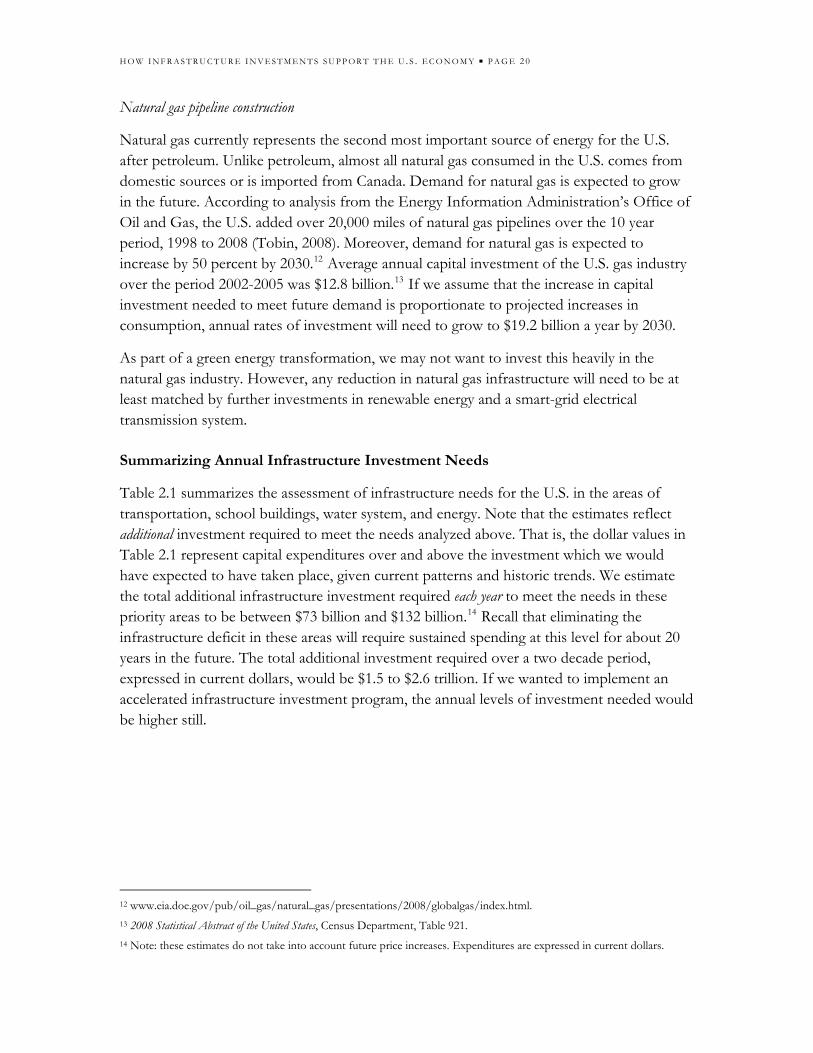
Summarizing Annual Infrastructure Investment Needs
Table 2.1 summarizes the assessment of infrastructure needs for the U.S. in the areas of transportation, school buildings, water system, and energy. Note that the estimates reflect additional investment required to meet the needs analyzed above. That is, the dollar values in Table 2.1 represent capital expenditures over and above the investment which we would have expected to have taken place, given current patterns and historic trends. We estimate the total additional infrastructure investment required each year to meet the needs in these priority areas to be between $73 billion and $132 billion.14 Recall that eliminating the infrastructure deficit in these areas will require sustained spending at this level for about 20 years in the future. The total additional investment required over a two decade period, expressed in current dollars, would be $1.5 to $2.6 trillion. If we wanted to implement an accelerated infrastructure investment program, the annual levels of investment needed would be higher still.
12 www.eia.doe.gov/pub/oil_gas/natural_gas/presentations/2008/globalgas/index.html. 13 2008 Statistical Abstract of the United States, Census Department, Table 921. 14 Note: these estimates do not take into account future price increases. Expenditures are expressed in current dollars.

H O W I N F R A S T R U C T U R E I N V E S T M E N T S S U P P O R T T H E U . S . E C O N O M Y ■ P A G E 2 1
Table 2.1. Summary of additional annual infrastructure investment needs.
cost (billions of dollars) primary source
transportation infrastructure
roads and bridges + $8.5 – 61.4 public rail + $5.3 private aviation + $3.2 public/private mass transit + $3.2 – 9.2 public inland waterways + $6.2 public total transportation +$26.4 – 85.3 --- public school buildings + $4.7 public water infrastructure
drinking water + $8.0 public wastewater systems + $7.4 public dams +$0.8 public total water $16.2 --- energy infrastructure
electricity (including renewables) $45.0 private natural gas $12.8-19.2 private total energy $25.7 --- ESTIMATE OF TOTAL ADDITIONAL INFRASTRUCTURE INVESTMENT NEEDS15
$73 – 132 billion ---
The “+” represents infrastructure needs in addition to actual expected expenditures.
With this assessment of infrastructure needs, we can propose scenarios for an expanded investment program that would help to close the infrastructure deficit to different degrees and over longer or shorter periods of time. These policy scenarios can be evaluated in terms of economic impacts. As this review has suggested, precise and detailed information on the future infrastructure needs for the U.S. are not always readily available. Therefore, we use this assessment to illustrate the employment impact of a program of accelerated investment without claiming that the mix of infrastructure investments used is necessarily the ‘right’ one. With this caveat in mind, we examine two possible infrastructure investment scenarios and estimate the number of jobs that would be created if such policies were implemented.
15 We estimate the increase in infrastructure investment required to meet current and future needs beyond the expected level of actual investment (based on historic patterns or other analysis). The estimates for gas and electricity represent total investment – not simply the additional investment required to meet demand in the future. For gas, recent levels of investment were $12.8 billion/year and we project this will need to increase to $19.2 billion/year by 2030. We estimate additional annual investment needs to be half of the difference of $6.4 billion, or $3.2 billion. For electricity, we note that the Edison Electric Institute estimates that investment in electricity transmission infrastructure totaled $37.8 billion from 2000 to 2006 ($6.3 billion a year) and will total $37 billion from 2007 to 2010 ($12.3 billion a year). This represents a doubling of annual investment from recent historical levels. Therefore, we assume that half of our assessment of electricity infrastructure needs represents required growth in investment over historical trends. See www.eei.org/industry_issues/energy_infrastructure/transmission/index.htm.
H O W I N F R A S T R U C T U R E I N V E S T M E N T S S U P P O R T T H E U . S . E C O N O M Y ■ P A G E 2 2
III. INFRASTRUCTURE INVESTMENT AND EMPLOYMENT: POLICY SCENARIOS AND ESTIMATES OF JOB CREATION
We now turn to the central issue of concern for this report: how many jobs would be created by an expanded infrastructure investment program designed to substantially reduce, if not eliminate altogether, the country’s infrastructure deficit over time? Specifically, we construct two policy scenarios, each reflecting a different level of commitment to increasing infrastructure investment. Based on the levels of spending in each scenario, we then show how much employment each scenario will generate. We then compare this level of employment expansion with the jobs that would be created through the same dollar amount devoted to a program of tax reductions aimed at increasing household consumption. We specifically detail the impact on manufacturing employment and illustrate the importance of domestic production in any large-scale infrastructure program.
Sources of job creation
Before moving into considering various policy scenarios and related employment project-ions, it will be useful to review the methodology we use to generate employment estimates
To begin with, there are three sources of job creation associated with any expansion of spending, including an expansion in infrastructure investment. These are: 1. Direct effects: the jobs created by the production of the infrastructure itself (e.g. road construction jobs); 2. Indirect effects: the new jobs associated with increased demand for materials, goods, and services used in the construction of infrastructure (e.g. steel production and fabrication); 3. Induced effects: the expansion of employment that results when people who get jobs gener-ated by the direct and indirect effects spend their incomes on goods and services (e.g. retail).
Our estimates include only the jobs created by an increase in infrastructure investment. We do not attempt to estimate ancillary jobs associated with the operation and maintenance of the infrastructure once it is in place (e.g. street cleaners, operators of pipelines, bus drivers).
We begin by focusing first on direct and indirect effects. Direct and indirect effects are fairly straightforward to measure within the framework of our employment model, based on U.S. input-output accounts. Estimating induced effects involves a broader set of considerations operating throughout the entire economy. Therefore, we will consider the question of induced effects separately below.
Input-Output Model for Estimating Direct and Indirect Job Creation
Our primary tool for generating estimates of the employment impacts of infrastructure spending is a model based on the national input-output tables. In the technical appendix, we present an extended discussion of the methodology we used to build and analyze the input-output model. Here we present a brief non-technical summary of this discussion.

H O W I N F R A S T R U C T U R E I N V E S T M E N T S S U P P O R T T H E U . S . E C O N O M Y ■ P A G E 2 3
The input-output model captures in great detail the relationships that exist between different industries in the production of goods and services. We also observe the interconnections between consumers of goods and services, including households and governments, and the various producing industries. The input-output modeling approach enables us to estimate the effects on employment resulting from an increase in final demand for the products of a given industry. For example, we can estimate the number of jobs directly created in the fabricated metals industry for each $1 billion of spending on fabricated metal products. We can also estimate the jobs that are indirectly created in other industries through the $1 billion in spending on fabricated metals—including industries such as business services and steel. Overall, the input-output model allows us to estimate the economy-wide employment impacts from a given level of spending in a particular area.
The estimates from the input-output model also take into account leakages. The most important source of leakages for the kinds of investment we consider in this report is the use of imported goods and services in the production of infrastructure. Spending on imports does not raise the demand for domestic output and therefore does not create additional jobs. The estimates we present in this report take into account import leakages, given the actual level of imports which U.S. businesses and households purchase. As we will show later, the employment impacts would be larger if the share of domestic production were to increase.
In many cases, the industrial categories used to construct the input-output models correspond directly to particular areas of infrastructure delivery—e.g. heavy and civil construction. However, in other cases, single industrial categories are not sufficient to fully capture certain areas of infrastructure investment. A case in point is investment in renewable power generation, such as wind or solar. In order to estimate employment impacts in these industries, we had to construct synthetic ‘industries’ by combining components of industries that are now included in the government accounts. For example, we have created within the model a representation of the solar industry which consists of a combination of electrical equipment, components manufacturing, hardware, construction, and technical services. We have assigned relative weights to each of these industries in terms of their contributions based on profiles drawn from industry sources. Once this new category is developed, we are able to estimate the employment effects that would result from increased spending on solar investments, just as we estimate employment effects from building new roads.
Once we have the defined the industrial categories associated with the different categories of infrastructure investment, the calculation of employment effects comes directly from the input-output model itself. The model allows us to compute direct and indirect ‘employment multipliers’—that is, how many jobs are generated by a given level of spending in each infrastructure category. This kind of analysis forms the basis of the employment projections which we present in this section of the report.

H O W I N F R A S T R U C T U R E I N V E S T M E N T S S U P P O R T T H E U . S . E C O N O M Y ■ P A G E 2 4
Estimating induced job creation
It is more difficult to estimate the size of the induced employment effects—or what, within standard macroeconomic models, is commonly termed the consumption multiplier—than to estimate direct and indirect effects. The induced effects represent a somewhat different category of multiplier in that they capture the increase in employment that occurs when the income generated by the direct and indirect job creation is spent.
There are aspects of the induced effects which we can estimate with a high degree of confi-dence. In particular, we have a good sense of what is termed the ‘consumption function’—what percentage of the additional money people receive from being newly employed will be spent. But we cannot know with an equivalent degree of confidence what the overall employment effects will always be of that extra spending. To begin with, the magnitude of the induced effect will depend on existing conditions in the economy. If unemployment is high, this will mean that there are a good number of people able and willing to take jobs if new job opportunities open up. But if unemployment is low, there will be less room for employment to expand, even if newly employed people have more money to spend.
Similarly, if there is slack in the economy’s physical resources, the capacity to expand employment will be greater—and the induced effects larger. If the economy is operating at a high level of activity there is not likely to be a large employment gain beyond what resulted from the initial direct and indirect effects. Given the rapid deterioration of economic conditions over the past several months—including rapidly rising rates of unemployment—the U.S. economy is not likely to bump up against this kind of capacity constraint in the near future and we would expect the induced effects to be significant in the current climate. However, the uncertainty about the length and severity of the crisis makes it difficult to pinpoint the magnitude of induced effects with a high degree of accuracy.
A 2002 survey article by economists at the International Monetary Fund provides a useful summary of the types of factors that will be significant in determining whether induced effects are likely to be large or small (Hemming, Kell, and Mahfouz, 2002). These factors include the following: 1. There is excess capacity in terms of labor and productive equipment; 2. The spending increase will be focused on the domestic economy, with little of the additional spending going to imports; 3. The increase in government spending will both improve productivity, and will encourage (‘crowd in’) private investment, not act as a substitute that ‘crowds out’ private investment;16 4. Inflation is not likely to increase to unsustainable levels as a result of increased spending.
Given the severe economic downturn that the U.S. economy is now experiencing, all of these conditions are likely to hold. But we have developed a formal model to estimate more systematically the broad magnitude of the induced employment effects. We present the
16 We address this issue in greater detail in the subsequent section of this report.
H O W I N F R A S T R U C T U R E I N V E S T M E N T S S U P P O R T T H E U . S . E C O N O M Y ■ P A G E 2 5
details of our procedure in the appendix. The basic approach is straightforward. We begin by estimating how much of the additional employment income earned as a result of the increased infrastructure investments is spent on household consumption. Using our basic input-out model, we then estimate the number of jobs that this additional consumption spending would generate, assuming that there is ample excess capacity in the economy due to the prevailing high levels of unemployment. We find that for each $1 million in employment income which is generated through the direct and indirect effects, the induced effects will create, on average, an additional 9.2 jobs.
Employment estimates for infrastructure investments
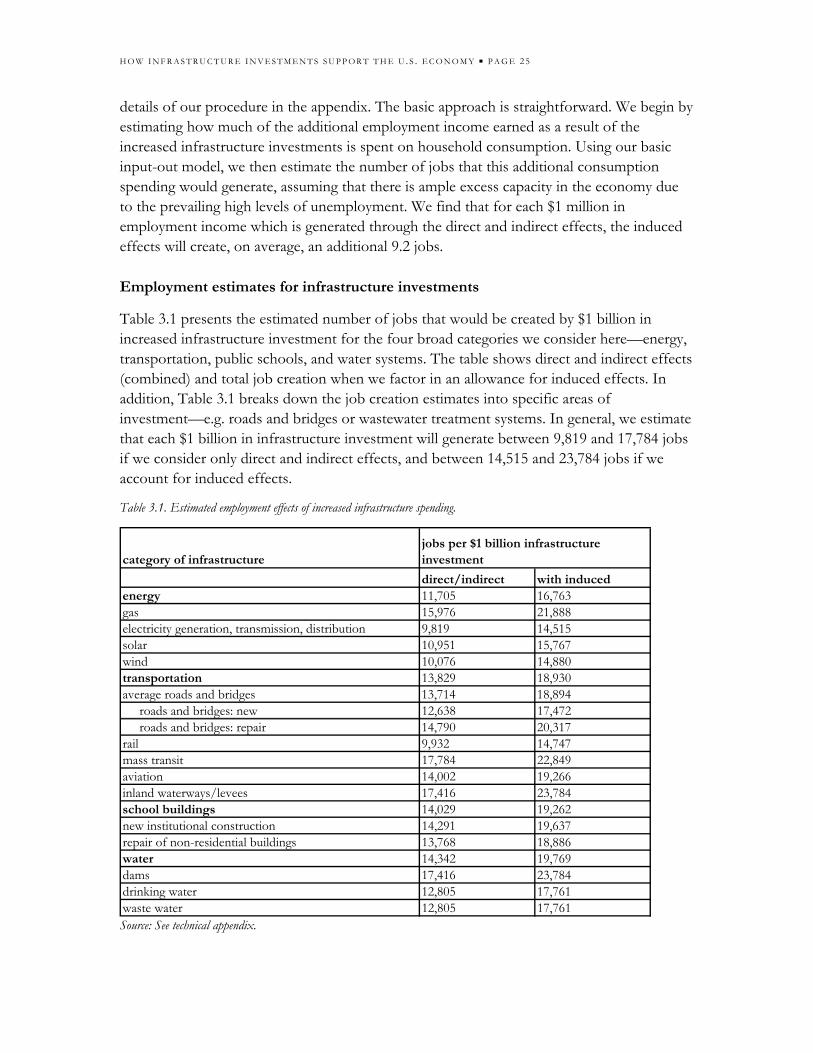
Table 3.1 presents the estimated number of jobs that would be created by $1 billion in increased infrastructure investment for the four broad categories we consider here—energy, transportation, public schools, and water systems. The table shows direct and indirect effects (combined) and total job creation when we factor in an allowance for induced effects. In addition, Table 3.1 breaks down the job creation estimates into specific areas of investment—e.g. roads and bridges or wastewater treatment systems. In general, we estimate that each $1 billion in infrastructure investment will generate between 9,819 and 17,784 jobs if we consider only direct and indirect effects, and between 14,515 and 23,784 jobs if we account for induced effects.
Table 3.1. Estimated employment effects of increased infrastructure spending.
direct/indirect with inducedenergy 11,705 16,763gas 15,976 21,888electricity generation, transmission, distribution 9,819 14,515solar 10,951 15,767wind 10,076 14,880transportation 13,829 18,930average roads and bridges 13,714 18,894 roads and bridges: new 12,638 17,472 roads and bridges: repair 14,790 20,317rail 9,932 14,747mass transit 17,784 22,849aviation 14,002 19,266inland waterways/levees 17,416 23,784school buildings 14,029 19,262new institutional construction 14,291 19,637repair of non-residential buildings 13,768 18,886water 14,342 19,769dams 17,416 23,784drinking water 12,805 17,761waste water 12,805 17,761
category of infrastructurejobs per $1 billion infrastructure investment
Source: See technical appendix.
H O W I N F R A S T R U C T U R E I N V E S T M E N T S S U P P O R T T H E U . S . E C O N O M Y ■ P A G E 2 6
The number of jobs created varies depending on the category of infrastructure in question. The highest direct and indirect employment impacts are associated with investments in mass transit systems; the lowest with investment in electricity production, transmission, and distribution infrastructure. However, the point of this exercise is not simply to rank the various categories of infrastructure in terms of their relative employment effects. Our objective is to evaluate the employment outcomes of an integrated infrastructure investment program, one based on the assessment of needs we analyzed in the previous section.
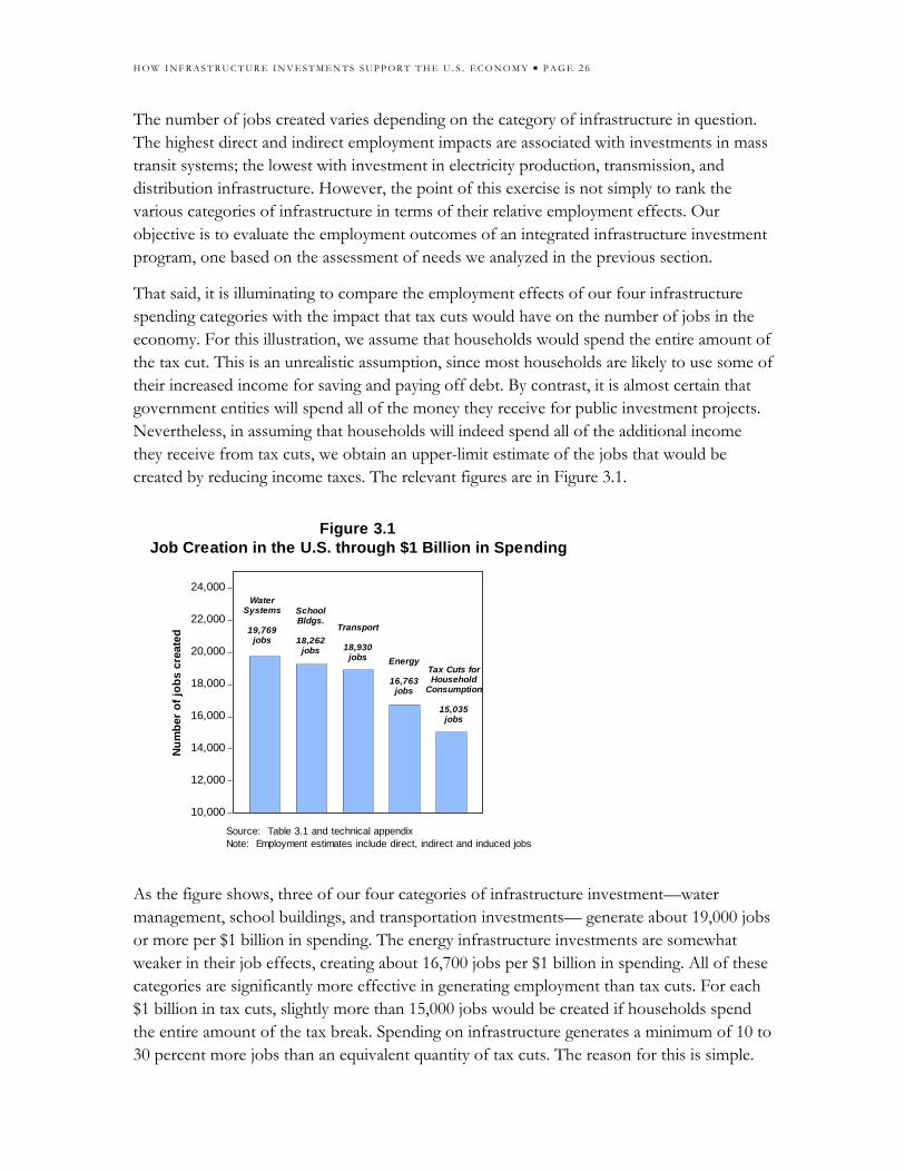
That said, it is illuminating to compare the employment effects of our four infrastructure spending categories with the impact that tax cuts would have on the number of jobs in the economy. For this illustration, we assume that households would spend the entire amount of the tax cut. This is an unrealistic assumption, since most households are likely to use some of their increased income for saving and paying off debt. By contrast, it is almost certain that government entities will spend all of the money they receive for public investment projects. Nevertheless, in assuming that households will indeed spend all of the additional income they receive from tax cuts, we obtain an upper-limit estimate of the jobs that would be created by reducing income taxes. The relevant figures are in Figure 3.1.
10,000
12,000
14,000
16,000
18,000
20,000
22,000
24,000
Figure 3.1Job Creation in the U.S. through $1 Billion in Spending
WaterSystems
19,769jobs
SchoolBldgs.
18,262jobs
Transport
18,930jobs Energy
16,763jobs
Tax Cuts forHousehold
Consumption
15,035jobs
Num
ber
of jo
bs c
reat
ed
Source: Table 3.1 and technical appendixNote: Employment estimates include direct, indirect and induced jobs
As the figure shows, three of our four categories of infrastructure investment—water management, school buildings, and transportation investments— generate about 19,000 jobs or more per $1 billion in spending. The energy infrastructure investments are somewhat weaker in their job effects, creating about 16,700 jobs per $1 billion in spending. All of these categories are significantly more effective in generating employment than tax cuts. For each $1 billion in tax cuts, slightly more than 15,000 jobs would be created if households spend the entire amount of the tax break. Spending on infrastructure generates a minimum of 10 to 30 percent more jobs than an equivalent quantity of tax cuts. The reason for this is simple.
H O W I N F R A S T R U C T U R E I N V E S T M E N T S S U P P O R T T H E U . S . E C O N O M Y ■ P A G E 2 7
Most of the spending on infrastructure investments goes towards purchasing domestically produced goods and services. Households spend a larger share of their income on imports, reducing the employment impact of tax cuts.
Infrastructure policy scenarios
To provide a range of job estimates for infrastructure spending, we propose two different infrastructure investment scenarios based on the infrastructure needs assessment—a baseline scenario and an accelerated, high-end scenario. In both cases, our focus is on additional infrastructure investment—that is, the amount by which capital spending on infrastructure would increase over the current level. In addition, we present these estimates as annual totals, although we would expect that a credible renewal program for the nation’s infra-structure would have to be a multi-year initiative. Of course, additional scenarios could be developed with different infrastructure priorities. The employment effects for any combina-tion of infrastructure investments can be calculated using the job creation estimates in Table 3.1. The employment effects would be scaled up based on the total level of spending.
The two scenarios were developed as follows:
Baseline scenario. We assume that the annual amounts in the basic needs assessment (Table 2.1) are met. For infrastructure categories with a range of possible investment needs (e.g. roads and mass transit), we double the lower-bound estimate (i.e. we double the ‘cost-to-maintain’ the current situation). In addition, we assume that 25 percent of the investment required to meet future electricity production needs would occur in renewable technologies —specifically, wind and solar. Capital investments in public schools and roads are divided into ‘new building’ and ‘repairs’ or ‘renovations’ based on industry estimates.17
High-end scenario. Here we envision an accelerated infrastructure investment program.18 For the road system, we assume total annual investment of $30.7 billion a year—half of the upper-limit in the needs assessment. For mass transit, we assume the full upper-end estimate of $9.2 billion is achieved. For both these categories, this level of investment goes well beyond the simple ‘cost-to-maintain’ assessment. In addition, we double the amount of investment in electricity transmission and distribution, renewable energy production, rail transportation, public schools, and water systems relative to the baseline scenario. Divisions between ‘new building’ and ‘repair/renovation’ are based on the same estimates used to construct the baseline scenario. For the remaining categories (aviation, natural gas, electricity
17 According to the Department of Transportation (2006) approximately 43 percent of public investment in roads went to expand the system and 57 percent when towards maintenance. Based on recent editions of the Annual Official Education Construction Report (ASU, 2007), we estimate that 45 percent of investment in public schools went towards renovations and 55 percent towards new building. 18 By ‘accelerated’ we mean one that would meet infrastructure needs more quickly than the 20 year time span used in several of the infrastructure areas analyzed in the assessment of needs to calculate annual levels of investment.

H O W I N F R A S T R U C T U R E I N V E S T M E N T S S U P P O R T T H E U . S . E C O N O M Y ■ P A G E 2 8
production—other than renewables, and inland waterways), we assume that the annual amounts in the basic needs assessment (Table 2.1) are met.
Table 3.2 summarizes the infrastructure investment scenarios. The baseline scenario proposes an additional $87 billion in increased infrastructure investment. However, as we have noted earlier, not all the categories of infrastructure are provided by the public sector. Of the $87 billion in additional investment, about $54 billion would represent increased public investment. The additional $33 billion in infrastructure spending would need to be mobilized by providing the private sector appropriate support and incentives.
Table 3.2. Infrastructure investment policy scenarios.
category of infrastructure
baseline highenergygas $3.2 $3.2electricity generation, transmission, dist. $20.2 $33.3solar $2.3 $4.7wind $2.3 $4.7transportationtotal roads and bridges $17.0 $30.7 roads and bridges: new $7.3 $13.2 roads and bridges: repair $9.7 $17.5rail $5.3 $10.6mass transit $6.4 $9.2aviation $3.2 $3.2inland waterways/levees $6.2 $6.2school buildingstotal school construction $4.7 $9.4new institutional construction $2.6 $5.2repair of non-residential buildings $2.1 $4.2waterdams $0.8 $1.6drinking water $8.0 $16.0waste water $7.4 $14.8
total $87.0 $147.6 public share $54.1 $92.8 private share $32.9 $54.7
Total public investment $271 $464
annual infrastructure investment($ billions)
TOTAL SPENDING
five year cost to public sector ($ billions)
Source: See text.
For the high-end, accelerated public investment scenario, the total annual increase would be an ambitious $147.6 billion, of which about $93 billion would be public. Of course, these levels of additional investment will help eliminate the infrastructure deficit only if they can be sustained over a number of years. Table 3.2 presents the level of public investment that would occur if the infrastructure investment scenarios were sustained over a five-year period.

H O W I N F R A S T R U C T U R E I N V E S T M E N T S S U P P O R T T H E U . S . E C O N O M Y ■ P A G E 2 9
How large are these proposals for increased infrastructure spending? One useful historic comparison is the creation of the federal interstate highway system. The massive expansion of roads, highways and bridges through this initiative fundamentally transformed the American economy. We would expect the kinds of infrastructure programs proposed here to have a similar impact. Therefore, it is instructive to look at the highway program in more detail, given the transformative potential of public investment.
The federal interstate highway program was first conceived in the 1930s, but began to be implemented under the Eisenhower administration following the Second World War. The first appropriations were planned in 1952 for the fiscal year 1954/5. From 1958 to 1991, periodic reports were made to Congress about the total cost of the interstate highway system. To compare the total costs of the federal highway system to the scenarios outlined here, we estimated the change in the costs of the highway system between the various years of the Congressional reports and adjusted for average price levels. We summed up the net additions to the highway system between each Congressional report and converted the annual investment figures into 2007 dollars. We estimate the total cost (in constant 2007 dollars) to have been approximately $530 billion.
The bulk of the current interstate highway system had been completed by the early 1980s. Therefore, we assume, for all intents and purposes, that the federal interstate highway system was built over the 24 year period 1958-1981 at a cumulative cost of $530 billion in 2007 dol-lars. This translates into approximately $22.2 billion in net public investment per year. This is significantly lower than the annual public investment in the baseline scenario. Of course in the scenarios, we are considering a range of infrastructure investment—not simply highways, roads, and bridges. If we restrict our attention to the road system, the interstate highway initiative, expressed in annual spending, was close in magnitude to our baseline scenario.
This suggests that our accelerated high-end investment scenario represents a public investment initiative that is significantly larger than the creation of the interstate highway system. Indeed, given the total public annual public investment of $92.8 billion associated with the accelerated scenario, the additional amount of public investment would total the $530 billion spent building the interstate highway system in just under six years. Despite the limitations of this comparative exercise, it does suggest that the baseline and accelerated scenarios represent ambitious infrastructure investment programs.
Employment effects of policy scenarios
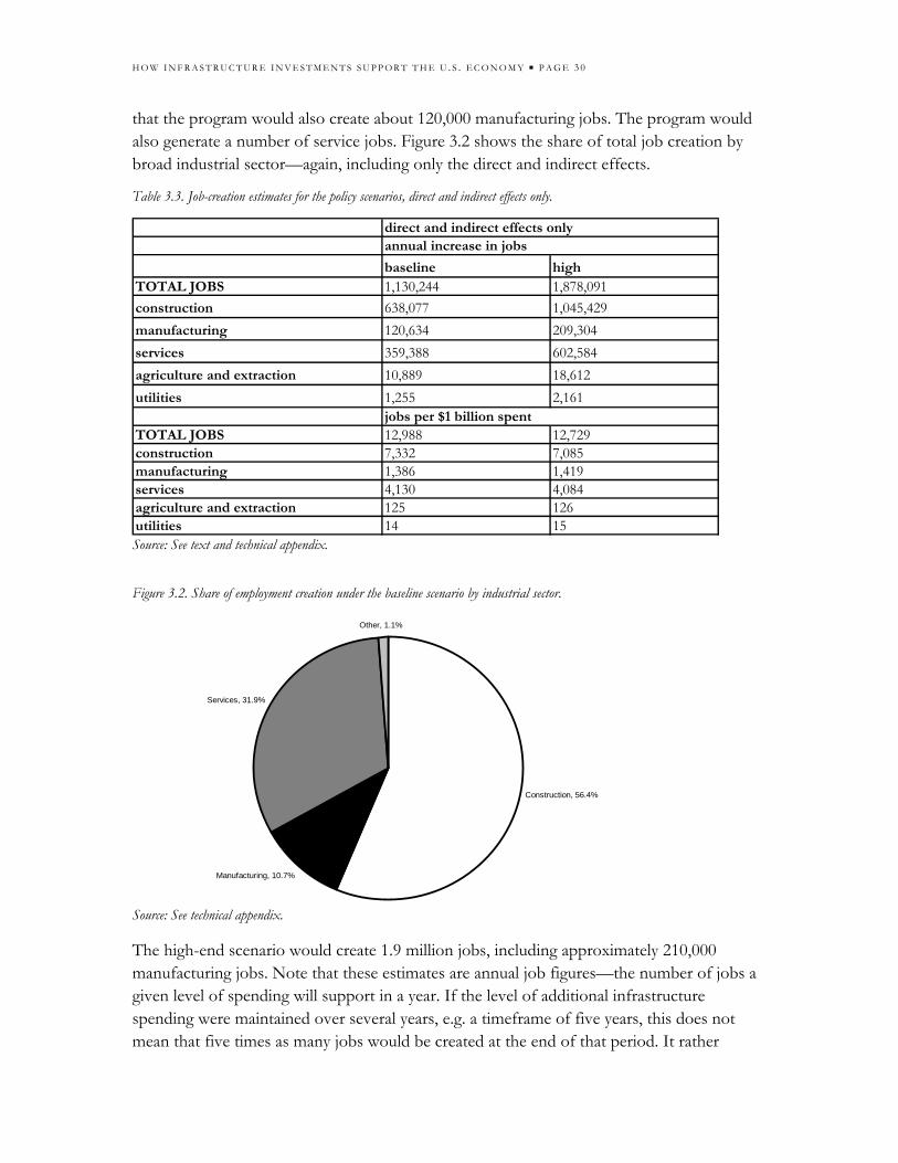
How many jobs would the different investment scenarios actually create? Table 3.3 summarizes the estimates—focusing only on the direct and indirect effects. The table also presents the number of jobs that would be generated for each $1 billion spent under the two scenarios. Looking first at the baseline scenario, we estimate that this infrastructure program would create slightly more than 1.1 million jobs through direct plus indirect effects. The largest number of jobs would be construction jobs—about 640,000. However, we project
H O W I N F R A S T R U C T U R E I N V E S T M E N T S S U P P O R T T H E U . S . E C O N O M Y ■ P A G E 3 0
that the program would also create about 120,000 manufacturing jobs. The program would also generate a number of service jobs. Figure 3.2 shows the share of total job creation by broad industrial sector—again, including only the direct and indirect effects.
Table 3.3. Job-creation estimates for the policy scenarios, direct and indirect effects only.
baseline highTOTAL JOBS 1,130,244 1,878,091construction 638,077 1,045,429manufacturing 120,634 209,304services 359,388 602,584agriculture and extraction 10,889 18,612utilities 1,255 2,161
TOTAL JOBS 12,988 12,729construction 7,332 7,085manufacturing 1,386 1,419services 4,130 4,084agriculture and extraction 125 126utilities 14 15
annual increase in jobsdirect and indirect effects only
jobs per $1 billion spent
Source: See text and technical appendix.
Figure 3.2. Share of employment creation under the baseline scenario by industrial sector.
Construction, 56.4%
Manufacturing, 10.7%
Services, 31.9%
Other, 1.1%
Source: See technical appendix.
The high-end scenario would create 1.9 million jobs, including approximately 210,000 manufacturing jobs. Note that these estimates are annual job figures—the number of jobs a given level of spending will support in a year. If the level of additional infrastructure spending were maintained over several years, e.g. a timeframe of five years, this does not mean that five times as many jobs would be created at the end of that period. It rather

H O W I N F R A S T R U C T U R E I N V E S T M E N T S S U P P O R T T H E U . S . E C O N O M Y ■ P A G E 3 1
means that the average annual level of job creation will be maintained over a longer time period—i.e. the additional jobs would last for five years instead of just a single year.
In Table 3.4, we report overall job-creation effects, including induced as well as direct plus indirect effects. Taking into account the induced effects, our estimate of total job creation under the baseline scenario is 1.6 million jobs, of which 146,000 would be in manufacturing. Our estimate of total job creation under the accelerated program would be 2.6 million jobs. In this high-end scenario, over a quarter of a million manufacturing jobs would be created.19
Table 3.4. Total estimated job creation for the policy scenarios, direct, indirect, and induced effects.
baseline high enddirect and indirect 1,130,244 1,878,091induced 445,254 746,908TOTAL JOBS 1,575,498 2,624,999
construction 640,987 1,050,310manufacturing 146,220 252,224services 761,929 1,277,842
TOTAL 18,104 17,791construction 7,366 7,118manufacturing 1,680 1,709services 8,755 8,660
annual number of jobs
Total employment by sector (including induced)
Employment per $1 billion spent
Source: See text and technical appendix.
Enough workers to fill the new jobs?
Of course, all of these estimates presume that there is enough slack in the labor market to allow room for this level of employment expansion. What would the impact of these programs be in the context of current employment conditions? The Bureau of Labor Statistics, in its December 2008 Employment Situation Summary, estimated that 11.1 million people were unemployed—corresponding to an unemployment rate of 7.2 percent. The baseline scenario would create 1.6 million jobs (including induced effects) in its first year. This increase of 1.6 million jobs would lower the unemployment rate to 6.2 percent. An increase of 2.6 million jobs associated with the accelerated, high-end scenario would reduce the unemployment rate to 5.5 percent. Thus, even with our accelerated infrastructure investment scenario, the level of unemployment would remain high. There are currently more than enough unemployed workers to take the new jobs without bumping up against labor supply problems or inflationary pressures.
19 These estimates for employment creation through infrastructure investment spending are much higher than the estimates reported in the January 9, 2009 document outlining the Obama economic recovery program, Romer and Bernstein, “The Job Impact of the American Recovery and Reinvestment Plan.” This report estimates that 377,000 jobs would be created through infrastructure investment spending that would be one component of an overall $775 billion stimulus program. We discuss the sources for these differences in our respective estimates in the technical appendix.
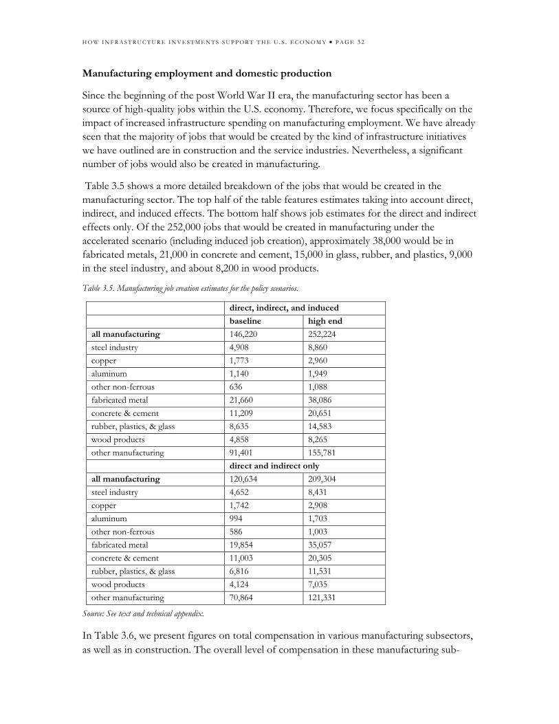
H O W I N F R A S T R U C T U R E I N V E S T M E N T S S U P P O R T T H E U . S . E C O N O M Y ■ P A G E 3 2
Manufacturing employment and domestic production
Since the beginning of the post World War II era, the manufacturing sector has been a source of high-quality jobs within the U.S. economy. Therefore, we focus specifically on the impact of increased infrastructure spending on manufacturing employment. We have already seen that the majority of jobs that would be created by the kind of infrastructure initiatives we have outlined are in construction and the service industries. Nevertheless, a significant number of jobs would also be created in manufacturing.
Table 3.5 shows a more detailed breakdown of the jobs that would be created in the manufacturing sector. The top half of the table features estimates taking into account direct, indirect, and induced effects. The bottom half shows job estimates for the direct and indirect effects only. Of the 252,000 jobs that would be created in manufacturing under the accelerated scenario (including induced job creation), approximately 38,000 would be in fabricated metals, 21,000 in concrete and cement, 15,000 in glass, rubber, and plastics, 9,000 in the steel industry, and about 8,200 in wood products.
Table 3.5. Manufacturing job creation estimates for the policy scenarios.
direct, indirect, and induced
baseline high end
all manufacturing 146,220 252,224 steel industry 4,908 8,860 copper 1,773 2,960 aluminum 1,140 1,949 other non-ferrous 636 1,088 fabricated metal 21,660 38,086 concrete & cement 11,209 20,651 rubber, plastics, & glass 8,635 14,583 wood products 4,858 8,265 other manufacturing 91,401 155,781 direct and indirect only
all manufacturing 120,634 209,304 steel industry 4,652 8,431 copper 1,742 2,908 aluminum 994 1,703 other non-ferrous 586 1,003 fabricated metal 19,854 35,057 concrete & cement 11,003 20,305 rubber, plastics, & glass 6,816 11,531 wood products 4,124 7,035 other manufacturing 70,864 121,331
Source: See text and technical appendix.
In Table 3.6, we present figures on total compensation in various manufacturing subsectors, as well as in construction. The overall level of compensation in these manufacturing sub-

H O W I N F R A S T R U C T U R E I N V E S T M E N T S S U P P O R T T H E U . S . E C O N O M Y ■ P A G E 3 3
sectors is roughly comparable to that within the construction sectors, with construction wages averaging $25.71 per hour, compared to the average wage for most of the manufacturing subsectors, which ranges between $21 – $28 per hour. The only exception is wood products, where average total compensation is slightly less than $20 per hour.
Table 3.6. Average hourly wages, benefits, and total compensation, selected industries.
median hourly wage median benefits (h l )
total hourly iconstruction $17.79 $7.92 $25.71
manufacturing subsectors
steel industry $18.42 $9.66 $28.08 copper $17.11 $8.97 $26.08 aluminum $17.00 $8.91 $25.91 other non-ferrous $18.04 $9.46 $27.50 fabricated metals $15.62 $8.19 $23.81 concrete & cement $15.47 $8.11 $23.58 rubber products $16.11 $8.45 $24.56 plastic products $13.89 $7.28 $21.17 glass products $15.41 $8.08 $23.49 wood products $13.05 $6.84 $19.89
Source: U.S. Bureau of Labor Statistics.
Imports and jobs
The job-creation impact of infrastructure projects will be sensitive to the relative proportion of total supplies that are imported from other countries. If imported goods are used to produce the kind of infrastructure we are discussing here, then the U.S. employment impact of increased investment will be lower. Imports represent a leakage from the domestic economy—the greater the leakages are, the less employment will be created for a given level of spending. This is not a serious concern for the construction and service industries. Most of the activities tied to construction and services are closely linked to the domestic economy and do not rely on imports. Given that about 90 percent of the total amount of economic activity generated by infrastructure investments will either be within the construction or service sectors, this in turn means that, overall, the level of imports generated by infrastructure investments will be low. At the same time, for the manufacturing sector, leakages from purchases of imported materials represent a more serious concern. We can see these effects in Tables 3.7 – 3.9.
Table 3.7 presents estimates of, respectively, the domestically produced and imported supplies used to produce the total output generated for different categories of infrastructure

H O W I N F R A S T R U C T U R E I N V E S T M E N T S S U P P O R T T H E U . S . E C O N O M Y ■ P A G E 3 4
investment.20 These figures take account of all supplies, or inputs, used in production, including labor, transportation, electricity and other energy sources, services from outside firms such as cleaning, legal and accounting support, as well as manufactured goods produced by both domestic and foreign businesses.
In general, as we see, the relative importance of domestic production for most of the categories of infrastructure investment is high—around 96-97 percent of total supplies purchased. Investments in energy infrastructure are the exception—particularly, investments in electricity, solar, and wind. In these cases, imports total nearly 11 percent of the value of output generated.
Table 3.7. Domestically produced and imported supplies for infrastructure investment projects (direct and indirect purchases only; does not include induced purchases)
U.S. made (%) imports (%)energy 89.4% 10.6%gas 97.3% 2.7%electricity generation, transmission, distribution 85.3% 14.7%solar 86.0% 14.0%wind 88.9% 11.1%transportation 96.8% 3.2%average roads and bridges 96.8% 3.2% roads and bridges: new 96.7% 3.3% roads and bridges: repair 96.9% 3.1%rail 96.9% 3.1%mass transit 96.7% 3.3%aviation 96.9% 3.1%inland waterways 97.3% 2.7%school buildings 96.9% 3.1%new institutional construction 97.1% 2.9%repair of non-residential buildings 96.7% 3.3%water 96.9% 3.1%waterways/levies/dams 97.3% 2.7%drinking water 96.8% 3.2%waste water 96.8% 3.2%
category of infrastructuredomestically produced and imported inputs (total direct and indirect effects)
Source: See technical appendix. Note: These figures take account of all supplies, or inputs, used in production, including labor, transportation, electricity and other energy sources, services from outside firms such as cleaning, legal and accounting support, as well as manufactured goods produced by both domestic and foreign businesses.
In Table 3.8, we focus on the relative breakdown of domestic supplies versus imports in considering the supplies from the manufacturing sector only to the overall infrastructure 20 By “total output” here, we are referring to direct plus indirect effects. We focus on these two effects because we are considering here only the effects of infrastructure investments themselves, not the effects of increases in consumption spending, as reflected in induced effects.
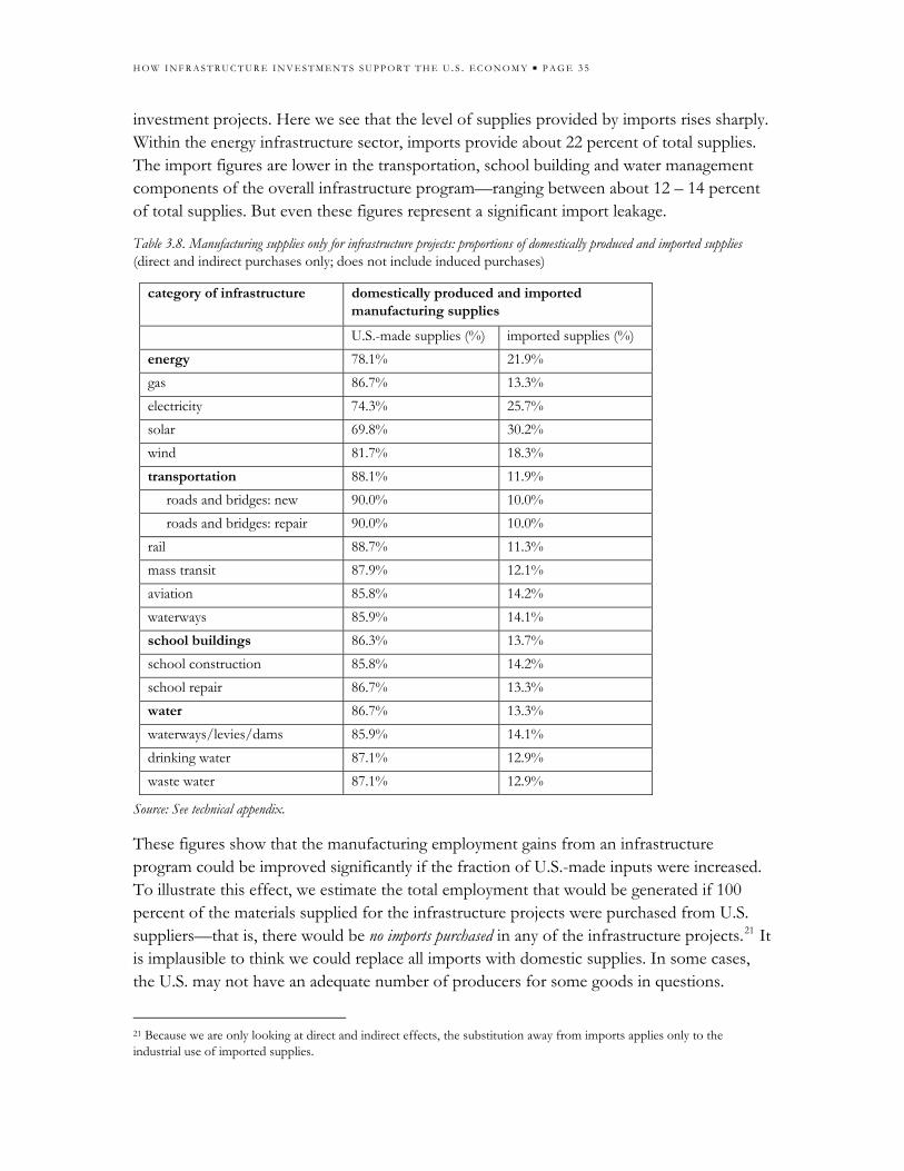
H O W I N F R A S T R U C T U R E I N V E S T M E N T S S U P P O R T T H E U . S . E C O N O M Y ■ P A G E 3 5
investment projects. Here we see that the level of supplies provided by imports rises sharply. Within the energy infrastructure sector, imports provide about 22 percent of total supplies. The import figures are lower in the transportation, school building and water management components of the overall infrastructure program—ranging between about 12 – 14 percent of total supplies. But even these figures represent a significant import leakage.
Table 3.8. Manufacturing supplies only for infrastructure projects: proportions of domestically produced and imported supplies (direct and indirect purchases only; does not include induced purchases)
category of infrastructure domestically produced and imported manufacturing supplies
U.S.-made supplies (%) imported supplies (%) energy 78.1% 21.9% gas 86.7% 13.3% electricity 74.3% 25.7% solar 69.8% 30.2% wind 81.7% 18.3% transportation 88.1% 11.9% roads and bridges: new 90.0% 10.0% roads and bridges: repair 90.0% 10.0% rail 88.7% 11.3% mass transit 87.9% 12.1% aviation 85.8% 14.2% waterways 85.9% 14.1% school buildings 86.3% 13.7% school construction 85.8% 14.2% school repair 86.7% 13.3% water 86.7% 13.3% waterways/levies/dams 85.9% 14.1% drinking water 87.1% 12.9% waste water 87.1% 12.9%
Source: See technical appendix.
These figures show that the manufacturing employment gains from an infrastructure program could be improved significantly if the fraction of U.S.-made inputs were increased. To illustrate this effect, we estimate the total employment that would be generated if 100 percent of the materials supplied for the infrastructure projects were purchased from U.S. suppliers—that is, there would be no imports purchased in any of the infrastructure projects.21 It is implausible to think we could replace all imports with domestic supplies. In some cases, the U.S. may not have an adequate number of producers for some goods in questions.
21 Because we are only looking at direct and indirect effects, the substitution away from imports applies only to the industrial use of imported supplies.
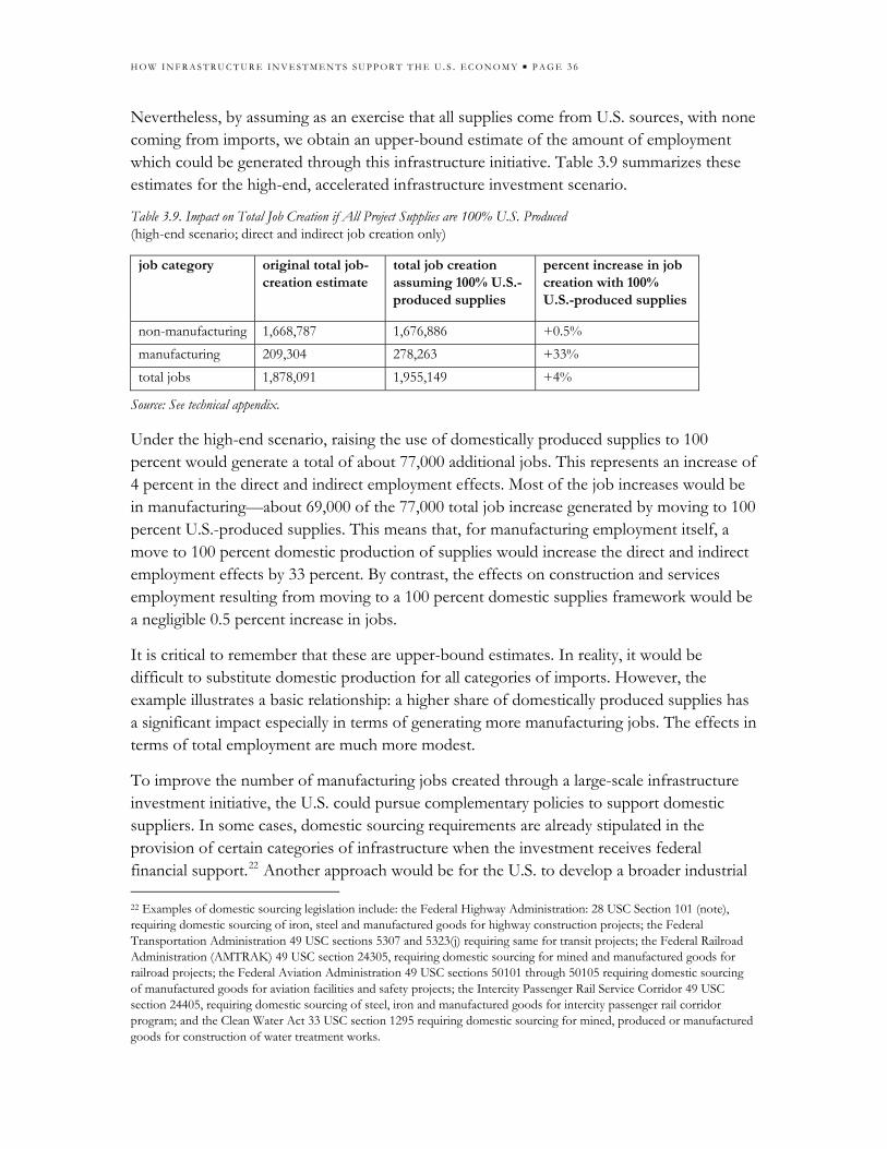
H O W I N F R A S T R U C T U R E I N V E S T M E N T S S U P P O R T T H E U . S . E C O N O M Y ■ P A G E 3 6
Nevertheless, by assuming as an exercise that all supplies come from U.S. sources, with none coming from imports, we obtain an upper-bound estimate of the amount of employment which could be generated through this infrastructure initiative. Table 3.9 summarizes these estimates for the high-end, accelerated infrastructure investment scenario.
Table 3.9. Impact on Total Job Creation if All Project Supplies are 100% U.S. Produced (high-end scenario; direct and indirect job creation only)
job category original total job-creation estimate
total job creation assuming 100% U.S.-produced supplies
percent increase in job creation with 100% U.S.-produced supplies
non-manufacturing 1,668,787 1,676,886 +0.5% manufacturing 209,304 278,263 +33% total jobs 1,878,091 1,955,149 +4%
Source: See technical appendix.
Under the high-end scenario, raising the use of domestically produced supplies to 100 percent would generate a total of about 77,000 additional jobs. This represents an increase of 4 percent in the direct and indirect employment effects. Most of the job increases would be in manufacturing—about 69,000 of the 77,000 total job increase generated by moving to 100 percent U.S.-produced supplies. This means that, for manufacturing employment itself, a move to 100 percent domestic production of supplies would increase the direct and indirect employment effects by 33 percent. By contrast, the effects on construction and services employment resulting from moving to a 100 percent domestic supplies framework would be a negligible 0.5 percent increase in jobs.
It is critical to remember that these are upper-bound estimates. In reality, it would be difficult to substitute domestic production for all categories of imports. However, the example illustrates a basic relationship: a higher share of domestically produced supplies has a significant impact especially in terms of generating more manufacturing jobs. The effects in terms of total employment are much more modest.
To improve the number of manufacturing jobs created through a large-scale infrastructure investment initiative, the U.S. could pursue complementary policies to support domestic suppliers. In some cases, domestic sourcing requirements are already stipulated in the provision of certain categories of infrastructure when the investment receives federal financial support.22 Another approach would be for the U.S. to develop a broader industrial 22 Examples of domestic sourcing legislation include: the Federal Highway Administration: 28 USC Section 101 (note), requiring domestic sourcing of iron, steel and manufactured goods for highway construction projects; the Federal Transportation Administration 49 USC sections 5307 and 5323(j) requiring same for transit projects; the Federal Railroad Administration (AMTRAK) 49 USC section 24305, requiring domestic sourcing for mined and manufactured goods for railroad projects; the Federal Aviation Administration 49 USC sections 50101 through 50105 requiring domestic sourcing of manufactured goods for aviation facilities and safety projects; the Intercity Passenger Rail Service Corridor 49 USC section 24405, requiring domestic sourcing of steel, iron and manufactured goods for intercity passenger rail corridor program; and the Clean Water Act 33 USC section 1295 requiring domestic sourcing for mined, produced or manufactured goods for construction of water treatment works.

H O W I N F R A S T R U C T U R E I N V E S T M E N T S S U P P O R T T H E U . S . E C O N O M Y ■ P A G E 3 7
policy framework, aimed at promoting U.S. producers as world leaders in sustainable and efficient energy, such as solar, wind, and smart grid energy technologies. Direct ties to domestic manufacturing would be part of this broader industrial policy framework.
Overall picture of the U.S. labor market
We estimate that the baseline infrastructure investment program—consisting of a total of $87 billion in additional infrastructure investment each year—would generate a total of 1.6 million jobs each year, including approximately 150,000 manufacturing jobs. Within the context of the December 2008 labor market situation, this job expansion would be sufficient to bring the unemployment rate down to 6.2 percent—assuming that the economic situation does not deteriorate further. A more ambitious infrastructure program is required to make a larger impact on unemployment. In our accelerated, high-end scenario, involving an additional $148 billion in infrastructure investment each year, 2.6 million jobs would be created, including about 250,000 manufacturing jobs. Again, within the context of the December 2008 labor market, this level of job creation could reduce the unemployment rate to 5.5 percent. It should be noted that the level of infrastructure investment required for the accelerated program—particularly, public investment—represents a significant increase over current levels. Such a program would constitute a large-scale public invest- ment initiative in many respects more ambitious than the building of the interstate highway system from 1959-80.
The estimates contained in this section are largely short-run in nature. We have talked about the number of jobs that would be created each year and have framed the infrastructure programs in terms of a five-year time span. However, such investment programs are not simply a short-run stimulus packages. They also create new public assets that contribute to the long-run productivity of the U.S. economy. It is these long-run impacts that are the subject of the next section of this report.

H O W I N F R A S T R U C T U R E I N V E S T M E N T S S U P P O R T T H E U . S . E C O N O M Y ■ P A G E 3 8
IV. ‘CROWDING OUT’ VS. ‘CROWDING IN’: PUBLIC INVESTMENT AND PRIVATE-SECTOR PRODUCTIVITY
Probably the single most common and influential argument against increasing the level of public investment is that it will ‘crowd out’ private investment—i.e. an increase in public infrastructure spending will be associated with an equivalent decline in private investment. Why would this be the case? Investments in infrastructure require real economic resources—materials, equipment, and people’s labor. They also require financial resources—money coming either from tax revenues or government borrowing. The ‘crowding out’ argument assumes that when the public sector consumes more of these real and financial resources, it necessarily diminishes the amount available to the private sector. Therefore, an increase in public capital expenditures results in less private sector production. In other words, the ‘economic pie’ is fixed. When the government takes a bigger slice, it leaves less for the private economy.
However, even at the level of simple logic, the crowding out argument only holds under a specific set of narrow economic circumstances. These circumstances would be when: 1) all the economy’s real resources are being fully utilized, i.e. workers are fully employed, and the existing productive apparatus is being run full-tilt; 2) the economy’s financial resources are similarly already being fully used up in financing productive investment projects; and 3) new public investment spending makes no contribution toward expanding the economy’s productive capacity—i.e. it is not succeeding in its purpose of increasing the overall size of the economic pie.
In the current economic crisis, unemployment is rising toward its highest level in a genera-tion and financial institutions are providing almost no loans for private investment, prefer-ring instead to hoard huge cash reserves and to purchase U.S. Treasury bonds, the single safest asset available on financial markets. Under these circumstances, there is no possibility of public investment projects bidding resources away from the private sector. Rather, higher rates of public infrastructure will increase the total number of people who can find employ-ment, and it will put to good use the financial resources flowing into the U.S. Treasury.
But these are of course extraordinary circumstances. It is also important to recognize that crowding out need not occur even when the economy is booming and unemployment is low. This is because public infrastructure investments will expand the economy’s long-term productive capacity, with benefits flowing primarily to the private sector. Because public infrastructure investment actually increases the overall size of the economic pie, both the public and the private sectors can expand together through a complimentary, mutually-supportive growth path.
More specifically, public spending provides goods and services essential for private produc-tion, including roads, bridges, energy, water, aviation, and water transport. Infrastructure improvements can increase labor productivity—e.g. more efficient transportation systems to and from work reduce wasted time. Better infrastructure can also reduce fossil fuel
H O W I N F R A S T R U C T U R E I N V E S T M E N T S S U P P O R T T H E U . S . E C O N O M Y ■ P A G E 3 9
consumption specifically, and overall energy consumption more generally. This reduces greenhouse gas emissions, and thus the environmental barriers to economic growth.
Estimating public investment benefits for overall output growth
It is not difficult to offer these arguments as to the benefits of public infrastructure investment in broad generalities, but more difficult to demonstrate their validity through systematic statistical analyses. But it is crucial to be able to put these arguments to more formal tests. We therefore now turn to a formal statistical model to explore whether we can observe the anticipated positive gains from public investment spending through this formal approach.
In doing so, we begin by introducing the important research conducted in the 1980s and early 1990s, led by economists Alicia Munnell and David Aschauer. Working separately, Munnell and Aschauer both suggested that public investment in the United States economy contributes to better performance of the private economy in terms of higher productivity and employment expansion (Aschauer, 1989a, 1989b; Munnell 1990a, 1990b). That is, public investment actually raises the return on private investment—crowding in rather than crowding out private investment. Both Munnell and Aschauer suggested that the sharp decline in the growth of public investment, which we documented earlier, contributed to the declining trend in productivity growth in the 1970s and 1980s. A growing infrastructure deficit would drag down the productivity and competitiveness of the U.S. economy.
Numerous critiques of this earlier work were advanced, focusing on technical statistical matters. We briefly review these issues in the technical appendix. For the sake of the current discussion, it is sufficient to point out that the earlier work of Aschauer and Munnell did not fully address important properties of the data they used to generate their results, raising the possibility that the relationship they found between public investment and private economic performance was spurious. Critics argued that, once these problems were addressed, the statistical findings they had derived end up falling apart.
For the current study, we re-estimated these relationships using up-to-date data and addressed the statistical issues associated with earlier research. We evaluate the impact of public infrastructure investment on the productivity of the private economy (as a whole) and on the productivity of the manufacturing sector, specifically. Again, we leave the technical details of this exercise to the appendix. Here we simply summarize the main findings.
Throughout this report we have focused on total infrastructure investment, which has public and private components, with public investment including federal, state, and local government initiatives. For the purposes of this particular exercise, we narrow the focus of the analysis, with our specific concern being the impact of public investment on the private sector. We therefore exclude from our analysis the impact of the private components of infrastructure investments on overall economic performance. Sharpening our focus still further, we consider those categories of public infrastructure which would directly impact the production activities of the private sector. Therefore, we exclude categories of social

H O W I N F R A S T R U C T U R E I N V E S T M E N T S S U P P O R T T H E U . S . E C O N O M Y ■ P A G E 4 0
infrastructure—such as educational buildings, hospitals, and conservation areas from this statistical exercise. In terms of the four infrastructure investment scenarios presented in the previous section, this means we exclude investment in public schools but include all other areas of public investment. We refer to this narrower set of public investments—public investments in transportation, water and energy as ‘core public economic infrastructure.’
We found that sustained increases in core public economic infrastructure in the United States enhance the growth of private sector GDP by a substantial amount. Our results suggest that a sustained one-percentage point increase in the growth rate of core public economic infrastructure leads to an increase in the growth rate of private sector GDP of 0.6 percentage points. How significant is this gain in GDP growth?
We can see the effects with respect to our baseline and high-end public infrastructure investment spending programs. The relevant figures are shown in Table 4.1 As the table shows, if the baseline figure estimate of a $54 billion annual increase in total public infrastructure spending discussed in the previous section were achieved, this would raise the growth rate of private sector GDP by about 0.4 percentage points, which is equal to $45.6 billion in added net output within the private sector. A $46 billion gain in private sector GDP as of 2007 would translate into an annual productivity dividend of about $150 for every U.S. citizen, or $600 for a family of four. As we also see in Table 4.1, the $54 billion baseline increase in public infrastructure investment would also mean about $7.6 billion more output per year for the manufacturing sector alone.23
Table 4.1. Estimated effects of increases in public infrastructure investment on long-run private sector growth rates (based on 2007 infrastructure investment levels)
total private economy manufacturing only
increase in public infrastructure investment
percentage point increase in private GDP
total increase in private GDP
percentage point increase in manufacturing sector output
total increase in manufacturing output
baseline: $54 billion investment
+0.43% $45.6 billion +0.51% $7.6 billion
high-end: $93 billion investment increase
+0.73% $77.4 billion +0.88% $13.1 billion
Source: See text and technical appendix.
Table 4.1 also shows these growth dividend effects in terms of our high-end public infra-structure investment scenario. This would involve raising public infrastructure investments by $93 billion relative to the historic average of 1980 – 2007. With this additional $93 billion in public infrastructure investments, private sector GDP would increase by $77 billion annually. This would produce a productivity dividend of nearly $260 annually for every U.S. 23 Not all the assets involved in the increased infrastructure spending are public – for example, most of the assets of railroads, electric utilities, and gas companies are private. In addition, investment in public schools is excluded from the definition of ‘core economic infrastructure’ since the direct impacts on private sector are either difficult to measure or weak.

H O W I N F R A S T R U C T U R E I N V E S T M E N T S S U P P O R T T H E U . S . E C O N O M Y ■ P A G E 4 1
citizen. The manufacturing sector itself would grow correspondingly by an additional $13 billion per year.
It is important to recognize that these calculations capture the productivity impacts of core public infrastructure investments only, i.e. public infrastructure spending in transportation, water and energy. We have not included potential benefits from either school buildings or private-sector infrastructure investments. Therefore, the full benefits of the entire package of infrastructure improvements that we consider in this report will be higher than the estimates we present in this section. Also, it is critical to keep in mind that our analysis focuses only on the benefits in terms of increasing the growth rate of net output. We are not considering the benefits to families of better school buildings, shorter commutes or more effective levee systems. We also are not including here the environmental benefits of green public invest-ment areas, including mass transit, freight rail, and smart-grid electrical transmission systems.
Public infrastructure and U.S. competitiveness
As we have already discussed, the decline in public investment has been linked to slower growth in economic productivity, particularly during the 1970s and 1980s (Aschauer, 1989a; Munnell 1990a). Other researchers have shown that public investments have helped to reduce the cost of production in U.S. manufacturing (Nadiri and Mamuneas, 1994; Morrison and Schwartz, 1996). The results of our study—summarized above—also show that public investment improves private sector productivity, and the impact is proportionately larger for the manufacturing sector than for the private sector as a whole. All of this suggests that public investment in infrastructure will have a positive impact on the U.S. economy’s competitive position in the world—by raising productivity and reducing production costs.
It follows that a lack of decent infrastructure will hurt U.S. competitiveness and further undermine the performance of the manufacturing sector. Manufacturing businesses rely on public goods, such as transportation systems, to operate. Reliable, affordable, and sustainable sources of energy are also essential. Inefficient infrastructure raises costs and increases risks—all of which will compromise the competitive position of the economy. Therefore, the research results presented here affirm the importance of world-class infrastructure to maintain U.S. economic performance in this era of global integration.
Environmental effects of infrastructure investment program
The infrastructure investment program we have outlined here builds from the assessments of infrastructure needs developed by a range of public and private-sector agencies. These needs assessments, in turn, are targeted primarily at raising productivity throughout the economy and also, of course, improving our standards of public safety. These needs assessments are not specifically focused on addressing the challenges for economic policy posed by global warming and other serious environmental problems.

H O W I N F R A S T R U C T U R E I N V E S T M E N T S S U P P O R T T H E U . S . E C O N O M Y ■ P A G E 4 2
At the same time, strong connections do exist between the infrastructure program we have sketched and an investment program targeted at building a clean energy economy.24 Of course, not all categories of public investments are aimed at producing direct environmental benefits. Road construction projects are an obvious case in point. By the same token, not all green investments will promote either private productivity or employment. Moreover, some categories of green investments will be focused on public purposes other than energy conservation and clean energy sources.
For example, cleaning up brownfield sites will have strong environmental benefits, and will also create new private investment opportunities. But such investments do not directly create clean energy alternatives. Reforestation/afforestation will expand the overall supply of carbon sinks, thereby counteracting global warming. But such investments will not enhance private sector productivity.
The major infrastructure projects that do aim both to raise productivity and promote a clean energy economy include:
public transportation; freight rail; smart grid electrical transmission systems; and dams for hydroelectric power.
Thus, to the extent that these initiatives are priorities within a broader public infrastructure framework, we are thereby also strengthening the links between an infrastructure program and a clean energy agenda.
Beyond this, an effective infrastructure investment program can promote a clean energy economy simply through its beneficial effects on productively. Simply put, to raise the economy’s level of productivity means to produce more goods and services while consuming fewer supplies in the process of production. Energy is a major supply that is needed across industrial sectors. Thus, raising productivity, in many cases, can entail reducing overall energy consumption.
Conclusion
This study has examined the economic effects of a large-scale infrastructure investment program for the United States economy. We developed specific policy proposals based on assessments of the country’s infrastructure needs in four core areas—transportation, energy, water systems, and public school buildings. Within this framework, we focused primarily on two considerations in assessing the impact of these investment programs, i.e. economic growth and job creation. Our results demonstrate that the proposals can produce major benefits in terms of both job creation and economic growth. Productivity improvements are the channel through which economic growth—i.e. improvements in the country’s GDP
24 We have developed a short-term clean energy investment program in Pollin et al. (2008) Green Recovery http://www.peri.umass.edu/fileadmin/pdf/other_publication_types/peri_report.pdf.
H O W I N F R A S T R U C T U R E I N V E S T M E N T S S U P P O R T T H E U . S . E C O N O M Y ■ P A G E 4 3
growth rate—rises in response to infrastructure investments. We have also focused on how these economy-wide benefits will produce gains for the manufacturing sector specifically.
Despite the benefits that accrue through infrastructure investments, the core stock of U.S. infrastructure assets has been allowed to deteriorate badly over the past generation. Between 1950-79, public infrastructure investment and overall economic growth grew together at a healthy rate—infrastructure investment averaged 4.0 percent per year over this period while overall economic growth averaged 4.1 percent. However, from 1980 – 2007, the growth of public infrastructure fell sharply, to 2.3 percent per year, while overall economic growth averaged a tepid 2.9 percent.
We have shown that the decline in public infrastructure growth has been a significant factor causing the decline in overall economic growth. For example, we found that for the year 2007, public investment growth was 2.4 percent. If public investment had instead growth by 3.4 percent that year, then overall GDP would have been higher by $64 billion. The higher rate of infrastructure investment, in turn, would provide a $64 billion gain in GDP in 2007, which amounts to a dividend of $210 for every resident of the United States. The benefit would be on the order of $800 for a family of four.
But what exactly are the economy’s infrastructure needs? Based on our review of the literature of “needs assessments” developed by a range of both public and private agencies, we developed a baseline level of overall infrastructure needs totaling $87 billion per year, of which about $54 billion would come from the public and $33 billion would be private investment. We would anticipate a program of this magnitude would continue at least for five years to meet the country’s baseline infrastructure needs.
We then also developed a high-end assessment. Through this high-end program, the country’s infrastructure needs would be met more quickly and more fully than through the baseline program. Our high-end investment program totals $148 billion per year for the five-year time frame. Within this overall program, $93 billion would need to come from the public sector, while $55 billion would be private sector investments.
Building from the industrial surveys and input-output model developed by the U.S. Department of Commerce, we are able to estimate systematically the job-creation effects that would result from both our baseline- and high-end infrastructure programs. We show that, in general, the infrastructure investments in the core areas of transportation, water systems, energy, and school buildings will generate about 18,000 jobs for every $1 billion in spending. By contrast, a rise in household spending levels generated by a tax cut will create, at most, around 14,000 jobs per $1 billion in spending. This is 22 percent less than the job expansion generated by infrastructure investments.
In reality, this estimate for tax cuts is likely to be significantly weaker than our model would suggest, since households will probably use some of their increased income for saving and paying off debt rather than increasing their spending. Our estimate thus offers an upper-bound figure for the impact of tax cuts, by assuming, implausibly, that all the extra income

H O W I N F R A S T R U C T U R E I N V E S T M E N T S S U P P O R T T H E U . S . E C O N O M Y ■ P A G E 4 4
households receive through a tax cut will be used for increased spending. By contrast, in the case of money directly into public infrastructure projects, it is almost certain that government entities will spend all of the money they receive.
The main reason infrastructure investments create more jobs per $1 billion in spending than an increase in household consumption is that the share of spending that would be done within the U.S. economy—as opposed to the purchasing of imports—is significantly higher with infrastructure investments. As we show, the total amount of U.S.-based spending and purchases of supplies through investments in the areas of transportation, water management and school buildings will be as high as 97 percent of total spending, with only about three percent of spending going to imports. The proportion of domestically-based suppliers is significantly lower with energy infrastructure investments, at around 89 percent of total supplies purchased, with 11 percent of supplies provided by imports. But even this energy infrastructure investment figures is higher than the figure for U.S. consumption spending, in which imports amount to about 18 percent of total spending.
Based on these general findings, we show that our baseline infrastructure program will generate about 1.6 million new jobs within the United States and the high-end program will generate about 2.6 million jobs. The highest proportion of new jobs will be in the construction sector, which would capture about 40 percent of all the new job creation. This would amount to about 640,000 jobs under the baseline scenario and 1 million jobs under our high-end program.
The manufacturing sector would receive about 10 percent of the new jobs created through the infrastructure investment program. This would amount to about 146,000 jobs under the baseline scenario and 250,000 jobs under the high-end scenario. We also show that employment within manufacturing would benefit disproportionately if the infrastructure programs were to increase the proportion of their supply purchases from domestic sources as opposed to imports. If we allowed that fully 100 percent of all supplies came from domestic sources under our high-end scenario, overall employment would rise by about 77,000, or four percent of the total job creation generated by the high-end scenario. But manufacturing employment would gain 69,000 of the 77,000 in total employment gains, a rise of 33 percent for the manufacturing sector relative to the job growth that results if the current mix of domestic sourcing and import purchases remained unchanged.
Our focus in this study has been to give careful attention to the needs this country faces in terms of improving our infrastructure; and, in meeting those needs, establishing what the benefits will be for employment generation and overall economic growth. We have not focused in detail on the benefits that would accrue in terms of two additional crucial factors, i.e. U.S. competiveness and environmental protection. But when one does consider these additional benefits, the imperative before us becomes even more clear. This is to rebuild the country’s infrastructure, and thereby restore what has always been a key pillar of the country’s economic achievements.

H O W I N F R A S T R U C T U R E I N V E S T M E N T S S U P P O R T T H E U . S . E C O N O M Y ■ P A G E 4 5
DATA APPENDIX: STATE-LEVEL ESTIMATES OF PUBLIC INVESTMENT
Table A.1. State capital expenditures, 2006.
capital total capital as % of total
per capita public investment
public investment as % of state GDP
$ millions $ millions % dollars rank % rank Alabama $4,116 $48,675 8.5% $897 26 2.6% 15 Alaska $1,511 $14,886 10.1% $2,232 2 3.5% 1 Arizona $6,770 $59,005 11.5% $1,098 10 2.9% 6 Arkansas $1,873 $25,531 7.3% $667 48 2.1% 34 California $41,838 $503,694 8.3% $1,154 9 2.4% 18 Colorado $5,119 $51,201 10.0% $1,074 12 2.3% 24 Connecticut $2,958 $43,467 6.8% $846 32 1.4% 51 Delaware $1,114 $11,442 9.7% $1,306 6 1.9% 39 DC $1,891 $13,923 13.6% $3,232 1 2.1% 28 Florida $19,370 $194,056 10.0% $1,073 13 2.7% 10 Georgia $8,348 $87,002 9.6% $894 27 2.2% 25 Hawaii $866 $15,203 5.7% $677 47 1.5% 50 Idaho $1,070 $12,874 8.3% $731 45 2.2% 26 Illinois $10,863 $139,356 7.8% $850 31 1.9% 41 Indiana $4,848 $60,758 8.0% $769 40 2.0% 35 Iowa $3,172 $31,876 10.0% $1,067 14 2.6% 14 Kansas $2,605 $28,003 9.3% $945 22 2.4% 20 Kentucky $3,132 $40,724 7.7% $745 44 2.1% 29 Louisiana $4,298 $48,727 8.8% $1,013 18 2.1% 30 Maine $809 $14,783 5.5% $615 51 1.7% 46 Maryland $4,668 $61,099 7.6% $833 34 1.8% 42 Massachusetts $5,474 $85,425 6.4% $851 30 1.6% 48 Michigan $6,694 $106,268 6.3% $663 49 1.8% 44 Minnesota $5,299 $61,844 8.6% $1,028 17 2.2% 27 Mississippi $2,388 $30,507 7.8% $824 36 2.8% 7 Missouri $4,605 $54,574 8.4% $789 37 2.1% 32 Montana $926 $9,587 9.7% $977 20 2.9% 5 Nebraska $2,213 $21,139 10.5% $1,255 8 2.9% 3 Nevada $3,250 $25,966 12.5% $1,304 7 2.6% 13 New $989 $12,460 7.9% $754 41 1.8% 45 New Jersey $8,074 $114,427 7.1% $932 23 1.8% 43 New Mexico $1,716 $22,635 7.6% $884 28 2.4% 19 New York $28,328 $332,533 8.5% $1,469 4 2.8% 8 North Carolina $7,640 $88,765 8.6% $861 29 2.0% 36 North Dakota $690 $6,797 10.2% $1,083 11 2.7% 11 Ohio $10,296 $134,552 7.7% $898 25 2.3% 23 Oklahoma $2,691 $33,070 8.1% $752 42 2.1% 33 Oregon $3,513 $42,152 8.3% $952 21 2.3% 21 Pennsylvania $9,779 $143,817 6.8% $788 38 1.9% 38 Rhode Island $682 $13,338 5.1% $642 50 1.5% 49 South Carolina $4,002 $47,237 8.5% $924 24 2.7% 9 South Dakota $819 $7,189 11.4% $1,039 16 2.6% 16 Tennessee $4,544 $61,264 7.4% $748 43 1.9% 37 Texas $24,576 $221,507 11.1% $1,050 15 2.3% 22 Utah $2,606 $25,564 10.2% $1,010 19 2.7% 12 Vermont $441 $7,437 5.9% $710 46 1.9% 40 Virginia $6,338 $77,068 8.2% $830 35 1.7% 47 Washington $8,498 $78,082 10.9% $1,333 5 2.9% 4 West Virginia $1,396 $17,092 8.2% $772 39 2.5% 17 Wisconsin $4,692 $62,529 7.5% $842 33 2.1% 31 Wyoming $972 $8,240 11.8% $1,894 3 3.2% 2
Source: U.S. Census Bureau.

H O W I N F R A S T R U C T U R E I N V E S T M E N T S S U P P O R T T H E U . S . E C O N O M Y ■ P A G E 4 6
Table A.2. State per capita public investment (capital expenditures) by functional category, 2006.
education health highways natural resources
waste management
water systems
energy transit
Alabama $303 $81 $254 $33 $81 $10 $13 $1Alaska $467 $42 $1,021 $47 $52 $48 $77 $12Arizona $253 $5 $222 $136 $66 $73 $74 $72Arkansas $248 $17 $219 $13 $32 $52 $14 $1California $372 $27 $235 $55 $61 $100 $29 $24Colorado $281 $35 $205 $101 $56 $124 $23 $53Connecticut $281 $7 $148 $14 $26 $13 $1 $17Delaware $420 $14 $447 $58 $114 $19 $10 $3DC $183 $36 $78 $393 $641 $109 $0 $918Florida $318 $33 $319 $86 $36 $29 $34 $8Georgia $266 $24 $175 $37 $76 $81 $15 $23Hawaii $192 $6 $152 $55 $90 $24 $0 $5Idaho $203 $28 $282 $20 $48 $33 $3 $1Illinois $197 $5 $222 $74 $31 $29 $11 $82Indiana $230 $39 $220 $25 $56 $7 $9 $1Iowa $303 $46 $349 $48 $27 $33 $19 $4Kansas $218 $9 $391 $20 $49 $45 $25 $1Kentucky $221 $23 $254 $18 $20 $44 $5 $3Louisiana $163 $57 $316 $71 $49 $35 $24 $3Maine $162 $3 $252 $14 $20 $16 $0 $1Maryland $249 $4 $230 $109 $24 $16 $0 $35Massachusett $211 $11 $190 $22 $84 $61 $4 $76Michigan $287 $7 $142 $21 $53 $35 $6 $6Minnesota $261 $30 $357 $46 $45 $40 $14 $4Mississippi $236 $34 $358 $17 $23 $27 $4 $0Missouri $185 $39 $256 $42 $45 $25 $9 $36Montana $163 $8 $489 $55 $42 $34 $0 $4Nebraska $223 $12 $406 $48 $23 $67 $339 $0Nevada $372 $4 $328 $69 $21 $188 $1 $29New $273 $1 $170 $16 $18 $9 $0 $2New Jersey $316 $12 $224 $42 $40 $20 $1 $91New Mexico $315 $61 $264 $44 $26 $13 $1 $1New York $261 $75 $256 $27 $135 $21 $85 $325North $243 $34 $215 $47 $68 $51 $19 $31North $216 $3 $579 $66 $18 $50 $1 $0Ohio $278 $25 $220 $20 $110 $40 $6 $8Oklahoma $216 $8 $221 $27 $55 $30 $4 $9Oregon $198 $95 $245 $29 $80 $36 $14 $21Pennsylvania $217 $21 $274 $31 $43 $22 $6 $32Rhode Island $135 $4 $218 $9 $30 $30 $2 $13South $347 $89 $231 $23 $32 $52 $51 $1South $190 $9 $524 $43 $47 $43 $17 $1Tennessee $151 $30 $218 $17 $46 $56 $74 $3Texas $342 $18 $325 $26 $47 $60 $49 $16Utah $264 $26 $258 $45 $52 $80 $13 $47Vermont $322 $2 $199 $10 $28 $18 $11 $3Virginia $291 $15 $134 $38 $44 $34 $5 $7Washington $321 $39 $301 $57 $70 $51 $81 $137West $217 $6 $360 $7 $37 $58 $0 $5Wisconsin $187 $17 $337 $64 $43 $16 $14 $4Wyoming $463 $138 $647 $147 $69 $61 $6 $2
Source: U.S. Census Bureau.

H O W I N F R A S T R U C T U R E I N V E S T M E N T S S U P P O R T T H E U . S . E C O N O M Y ■ P A G E 4 7
Table A.3. Average growth rates of per capita public capital stock by state, 1966-2006.
1966-75 1976-85 1986-95 1996-2006 % growth rank % growth rank % growth rank % growth rankAlabama 3.6% 15 1.3% 25 1.0% 28 1.9% 7 Alaska 6.4% 3 3.5% 2 0.3% 44 0.3% 49 Arizona 1.6% 44 1.6% 16 0.9% 33 0.2% 51 Arkansas 3.8% 13 1.2% 29 0.7% 37 1.5% 21 California 1.6% 43 -1.0% 51 1.0% 25 1.9% 6 Colorado 1.4% 47 1.8% 13 1.7% 11 1.4% 24 Connecticut 2.5% 36 -0.2% 48 2.1% 4 1.1% 35 Delaware 3.5% 18 0.1% 47 -0.1% 51 1.1% 34 DC 8.7% 1 4.7% 1 1.4% 14 1.6% 20 Florida 0.7% 51 1.3% 26 2.1% 6 1.7% 14 Georgia 3.8% 14 2.2% 5 1.4% 16 1.2% 29 Hawaii 3.9% 9 0.4% 44 2.6% 1 0.2% 50 Idaho 1.7% 42 1.0% 36 1.0% 29 0.7% 47 Illinois 2.7% 31 1.5% 19 1.3% 17 1.8% 10 Indiana 3.1% 27 1.1% 30 1.2% 22 1.7% 17 Iowa 3.2% 25 2.1% 8 1.3% 21 1.7% 18 Kansas 2.5% 35 1.9% 11 0.6% 39 1.3% 25 Kentucky 3.6% 16 1.5% 21 0.8% 34 1.2% 30 Louisiana 2.4% 37 1.3% 27 1.0% 27 1.8% 8 Maine 3.3% 20 0.9% 39 1.6% 12 1.0% 41 Maryland 4.0% 7 1.9% 12 0.6% 40 0.7% 45 Massachusetts 4.0% 8 1.5% 20 2.1% 5 2.5% 1 Michigan 2.3% 38 0.9% 38 0.4% 43 1.7% 16 Minnesota 3.3% 22 1.4% 23 1.3% 20 1.4% 23 Mississippi 3.2% 24 0.8% 41 0.8% 35 1.9% 5 Missouri 3.2% 23 1.0% 34 1.1% 24 1.8% 12 Montana 2.8% 29 1.1% 31 0.3% 45 0.6% 48 Nebraska 4.6% 5 2.6% 3 0.5% 41 1.2% 28 Nevada 0.9% 50 -0.4% 50 0.0% 49 1.1% 38 New Hamp. 2.6% 32 0.2% 46 0.4% 42 1.1% 33 New Jersey 4.7% 4 1.4% 24 2.3% 3 1.8% 11 New Mexico 1.4% 48 1.3% 28 0.7% 36 1.1% 36 New York 3.9% 11 1.0% 35 2.0% 8 2.0% 4 North Carolina 3.9% 12 1.6% 18 1.9% 10 1.7% 15 North Dakota 2.6% 33 1.6% 17 1.3% 19 1.6% 19 Ohio 2.8% 30 1.4% 22 1.1% 23 2.2% 2 Oklahoma 1.7% 41 1.6% 15 1.6% 13 1.1% 40 Oregon 2.2% 39 1.1% 33 0.2% 47 1.5% 22 Pennsylvania 4.4% 6 0.9% 40 0.9% 30 1.8% 9 Rhode Island 3.3% 21 0.3% 45 2.0% 7 0.7% 46 South Carolina 3.9% 10 1.6% 14 2.4% 2 2.1% 3 South Dakota 3.0% 28 1.9% 10 0.7% 38 1.1% 39 Tennessee 3.1% 26 0.7% 43 0.9% 32 0.9% 42 Texas 2.1% 40 1.1% 32 1.4% 15 1.2% 31 Utah 1.2% 49 2.5% 4 0.2% 48 0.8% 43 Vermont 3.4% 19 -0.4% 49 -0.1% 50 0.7% 44 Virginia 3.6% 17 0.7% 42 1.3% 18 1.2% 27 Washington 1.5% 45 2.2% 7 0.3% 46 1.2% 32 West Virginia 7.3% 2 2.0% 9 0.9% 31 1.3% 26 Wisconsin 2.5% 34 0.9% 37 1.0% 26 1.8% 13 Wyoming 1.5% 46 2.2% 6 2.0% 9 1.1% 37 average 3.1% 1.3% 1.1% 1.3%
Source: See technical appendix.

H O W I N F R A S T R U C T U R E I N V E S T M E N T S S U P P O R T T H E U . S . E C O N O M Y ■ P A G E 4 8
TECHNICAL APPENDIX: METHODOLOGICAL TECHNIQUES AND DETAILS
A. Estimates of state-level public capital stock
The Bureau of Economic Analysis (BEA) of the U.S. Department of Commerce compiles national-level estimates of fixed capital stocks for the private and government sectors. This data is readily available on the BEA’s website (www.bea.gov) and is the source of the national level public stock data featured in this report. However, state-level estimates of public capital stock are not available. State-level data on capital expenditures are available for the U.S. Census Bureau as part of its State Government Finance program. However, this source only provides information on public capital expenditures by state, not on the state’s estimated capital stock.
As background for this report, we compiled state-level estimates of public capital stock using these two data sources. In so doing, we adapted the methodology first proposed by Alicia Munnell (1990b). Using the state-level data on capital expenditures from the Census Bureau, we construct proxy estimates of public capital stock by state. This proxy estimate consists of cumulative public investment, as measured by state-level capital spending among the various asset categories, adjusted for depreciation of public capital. This series includes both state and local governments. We used the methodology for calculating depreciation rates described in the BEA publication, Fixed Assets and Consumer Durable Goods in the United States, 1925-97 (published September 2003). Since the available census data only begins in 1957, our proxy capital stock measure is based on government capital expenditures from that time forward. Clearly, the public capital stock of the states pre-dates 1957. Therefore, our proxy measure, summed across all states, always is less than the BEA estimates of state and local government assets, although the two series converge over time.
To address the gap between our proxy measure and the BEA series on state and local government assets, we follow Munnell (1990b) and apportion the BEA public capital series using the individual state shares of public assets calculated from our proxy measure. For example, to calculate California’s capital stock, we multiply the BEA estimate of total state and local government fixed asset by California’s share of our proxy capital stock measure. In the early years, volatility in state spending causes the state shares (and hence our apportionment of the total capital stock) to vary excessively. However, this volatility dies down after several years. Therefore, we begin our estimates of state-level capital stock in 1965, since we feel that earlier estimates are not reliable.

H O W I N F R A S T R U C T U R E I N V E S T M E N T S S U P P O R T T H E U . S . E C O N O M Y ■ P A G E 4 9
B. The Input-Output Model and Employment Multipliers
1. The National Input-Output Model
Input-output tables (i.e. I-O tables) are compiled by the Bureau of Economic Analysis (BEA). Every five years the Census Department gathers data (in its “Economic Census”) and the BEA uses this data along with information from other Census programs—including annual surveys that cover selected industries, such as manufacturing and services. The I-O tables also incorporate data collected and tabulated by other Federal agencies—including the U.S. Departments of Agriculture, Education, and Energy—and data from a number of private organizations.25 The BEA uses the data collected from these various sources to construct benchmark input-output tables for approximately 500 industries. Between the quinquennial census years, the BEA updates the benchmark tables to produce annual input-output tables. These annual tables are available at the 13-industry level of detail as well as the 65-industry level of detail.
The BEA provides the make and use tables, as well as the direct requirements and total requirements tables. The total requirements table, or Leontief inverse matrix, shows how an increase in final demand for a particular industry’s product will lead to increased output in that industry and all related industries. For example, an increase in demand for farm products would increase farm output and would also increase output in other industries which provide inputs to the farm industry. In addition, we can calculate the domestic content and import requirements directly from the input-output tables.
To calculate the detailed employment impact assessments contained in this report, we used the social accounting and impact assessment software package, IMPLAN Pro (Version 2.0). IMPLAN is calibrated to the BEA I-O tables and includes a highly detailed level of industrial disaggregation—over 500 different sectors. Our input-output model is calibrated using 2006 data.
2. Using the Input-Output Model to Examine Employment Multipliers
To study the effects on employment using an I-O model, we also need to use employment/ output ratios. The assumption is that employment/output ratios remain fixed in the short-run. Therefore, output multipliers—derived from the Leontief inverse matrix—can be converted into employment multipliers by using the employment-output ratios. We use the IMPLAN software to perform these calculations at the 500 sector level of disaggregation.
The I-O model can also be used to calculate induced effects. The assumption is that a fixed proportion of the compensation employees receive is spent on household purchases. When total compensation goes up, household consumption (a category of final demand) increases proportionately. However, the I-O model of induced effects, computed by endogenizing the
25 Karen Horowitz and Mark Planting, “Concepts and Methods of the Input-Output Accounts,” Bureau of Economic Analysis, September 2006.

H O W I N F R A S T R U C T U R E I N V E S T M E N T S S U P P O R T T H E U . S . E C O N O M Y ■ P A G E 5 0
household sector, tends to generate implausibly large multiplier effects. Therefore, we do not use the direct I-O estimates of induced effects in our calculations but instead use a different methodology, described in the next section of the appendix.
3. Infrastructure spending and I-O employment multipliers
To perform the kind of employment analysis featured in this report we needed to match the infrastructure categories with the disaggregated sectors in order to calculate employment multipliers. In so doing, we had to focus on the provision of capital goods, not the delivery of services. For example, the industrial sector ‘oil and gas pipelines’ is associated with the operations of oil and gas transport, not capital investments. The construction of pipelines (other than water pipelines) is included in a category ‘civil and heavy construction.’ The details of how the infrastructure categories were matched with industrial sectors are contained in Table A.4.
Table A.4. Infrastructure categories and matching with industrial sectors in the I-O model.
infrastructure category industrial sector
gas pipelines civil and heavy construction (50% new, 50% repair) electricity 67% all electric power goods, 33% civil and heavy construction (see below) solar see text wind see text highways, roads, bridges bridges and roads—new, bridges and roads—repair rail rail construction mass transit mass transit construction
aviation 50% bridges and roads—new and repair (includes runways), 50% new institutional building construction (airport facilities)
public schools new institutional building construction, non-residential building repair.
wastewater water/sewer systems drinking water water/sewer systems dams and levees civil and heavy construction (repair only) inland waterways civil and heavy construction (repair only)
The solar and wind industries are composed of design, manufacturing and construction industries. The manufacturing industries reflect the components involved and the construction industry reflects the installation of solar panels and wind turbines. The composition of these industries is a weighted average of these industries, and the weights were chosen based on our reading of various industry journals and other publications. The weights for the wind industry were taken directly from one publication, the European Wind Energy Association’s “Wind Energy—The Facts,” published in 2004.

H O W I N F R A S T R U C T U R E I N V E S T M E N T S S U P P O R T T H E U . S . E C O N O M Y ■ P A G E 5 1
Using IMPLAN’s 2.0 software and 2006 data set, we analyzed the output and employment effects of each of these industries based on the weights and industries below.
Solar 0.300 Construction 0.175 Hardware manufacturing 0.175 Electrical equipment 0.175 Electrical components 0.175 Misc. professional, scientific and technical services
Wind 0.26 Construction 0.12 Plastic products 0.12Fabricated metal products 0.37Machinery 0.03 Mechanical power transmission 0.03 Electronic components 0.07 Misc. professional, scientific and technical services
For the estimates for the non-construction aspects of electrical infrastructure investment, we defined a category “all electric power goods.” This group contains the following industries (equally weighted):
All Electric Power Goods 0.20 Electric Power and specialty transformer manufacturing 0.20 Motor and generator manufacturing 0.20 Relay and industrial control manufacturing 0.20 Fiber optic cable manufacturing 0.20 other communication and energy wire manufacturing
This scheme for matching infrastructure provision to industrial categories was used in the generation of the employment estimates contained in the main text of the report.
C. Induced employment effects
Induced effects refer to the additional employment, output, and value-added that is produced when the additional employment income generated by an initial demand stimulus—as captured by the direct and indirect effects—is spent. The magnitude of the induced effects depends on how the additional employment income translates into household expenditures and the size of the multiplier effects associated with the increase in household spending.
Induced effects are often estimated by endogenizing the household sector in the input-output model. The assumption is that increases in employee compensation (or value added)
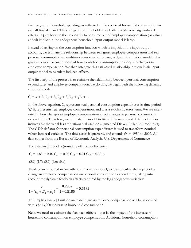
H O W I N F R A S T R U C T U R E I N V E S T M E N T S S U P P O R T T H E U . S . E C O N O M Y ■ P A G E 5 2
finance greater household spending, as reflected in the vector of household consumption in overall final demand. The endogenous household model often yields very large induced effects, in part because the propensity to consume out of employee compensation (or value-added) implicit in the endogenous household input-output model is large.
Instead of relying on the consumption function which is implicit in the input-output accounts, we estimate the relationship between real gross employee compensation and real personal consumption expenditures econometrically using a dynamic empirical model. This gives us a more accurate sense of how household consumption responds to changes in employee compensation. We then integrate this estimated relationship into our basic input-output model to calculate induced effects.
The first step of the process is to estimate the relationship between personal consumption expenditures and employee compensation. To do this, we begin with the following dynamic empirical model:
Ct = α + β1Ct-1 + β2Ct-2 + β3Ct-3 + γEt + μt
In the above equation, Ct represents real personal consumption expenditures in time period ‘t,’ Et represents real employee compensation, and μt is a stochastic error term. We are inter-ested in how changes in employee compensation affect changes in personal consumption expenditures. Therefore, we estimate the model in first differences. First differencing also insures that the variables are stationary (based on augmented Dickey-Fuller unit root tests). The GDP-deflator for personal consumption expenditures is used to transform nominal values into real variables. The time series is quarterly, and extends from 1950 to 2007. All data comes from the Bureau of Economic Analysis, U.S. Department of Commerce.
The estimated model is (rounding off the coefficients):
Ct = 7.83 + 0.10 Ct-1 + 0.20 Ct-2 + 0.21 Ct-3 + 0.30 Et
(3.2) (1.7) (3.5) (3.6) (5.9)
T-values are reported in parentheses. From this model, we can calculate the impact of a change in employee compensation on personal consumption expenditures, taking into account the dynamic feedback effects captured by the lag endogenous variables:
6132.05186.01
2952.0)(1 321
=−
=++− βββ
γ
This implies that a $1 million increase in gross employee compensation will be associated with a $613,200 increase in household consumption.
Next, we need to estimate the feedback effects—that is, the impact of the increase in household consumption on employee compensation. Additional household consumption
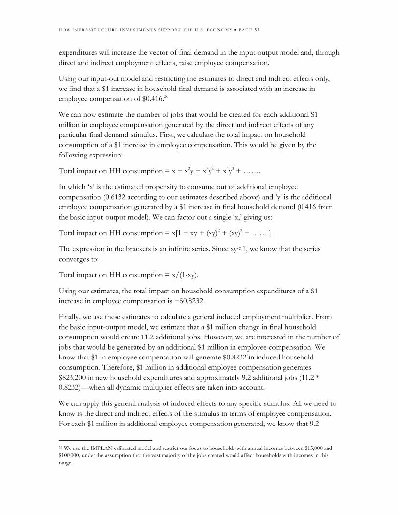
H O W I N F R A S T R U C T U R E I N V E S T M E N T S S U P P O R T T H E U . S . E C O N O M Y ■ P A G E 5 3
expenditures will increase the vector of final demand in the input-output model and, through direct and indirect employment effects, raise employee compensation.
Using our input-out model and restricting the estimates to direct and indirect effects only, we find that a $1 increase in household final demand is associated with an increase in employee compensation of $0.416.26
We can now estimate the number of jobs that would be created for each additional $1 million in employee compensation generated by the direct and indirect effects of any particular final demand stimulus. First, we calculate the total impact on household consumption of a $1 increase in employee compensation. This would be given by the following expression:
Total impact on HH consumption = x + x2y + x3y2 + x4y3 + …….
In which ‘x’ is the estimated propensity to consume out of additional employee compensation (0.6132 according to our estimates described above) and ‘y’ is the additional employee compensation generated by a $1 increase in final household demand (0.416 from the basic input-output model). We can factor out a single ‘x,’ giving us:
Total impact on HH consumption = x[1 + xy + (xy)2 + (xy)3 + …….]
The expression in the brackets is an infinite series. Since xy<1, we know that the series converges to:
Total impact on HH consumption = x/(1-xy).
Using our estimates, the total impact on household consumption expenditures of a $1 increase in employee compensation is +$0.8232.
Finally, we use these estimates to calculate a general induced employment multiplier. From the basic input-output model, we estimate that a $1 million change in final household consumption would create 11.2 additional jobs. However, we are interested in the number of jobs that would be generated by an additional $1 million in employee compensation. We know that $1 in employee compensation will generate $0.8232 in induced household consumption. Therefore, $1 million in additional employee compensation generates $823,200 in new household expenditures and approximately 9.2 additional jobs (11.2 * 0.8232)—when all dynamic multiplier effects are taken into account.
We can apply this general analysis of induced effects to any specific stimulus. All we need to know is the direct and indirect effects of the stimulus in terms of employee compensation. For each $1 million in additional employee compensation generated, we know that 9.2
26 We use the IMPLAN calibrated model and restrict our focus to households with annual incomes between $15,000 and $100,000, under the assumption that the vast majority of the jobs created would affect households with incomes in this range.

H O W I N F R A S T R U C T U R E I N V E S T M E N T S S U P P O R T T H E U . S . E C O N O M Y ■ P A G E 5 4
additional jobs would be generated through induced effects. For example, an additional $10 million spent on water systems infrastructure generates $5.38 million in additional employee compensation through the direct and indirect effects. These direct and indirect effects would generate about 128 new jobs. These numbers come directly from the basic input-output model. The induced job creation—taking into account all multiplier effects—would amount to approximately 49 additional jobs (5.38*9.2) for a total employment impact of 177 jobs.
D. Public investment in core economic infrastructure and private productivity
Research studies in the late1980s and early 1990s presented results which suggested that U.S. public investment improves private sector productivity (Aschauer 1989a, 1989b; Munnell 1990a, 1990b). The most damning criticism of these studies is that they failed to address the possibility that the results were spurious due to the presence of unit roots in key variables. Others researchers have established that the relevant variables, at least in the case of the U.S., are non-stationary (Tatom 1991; Sturm and Haan 1995). These studies find that when the relevant variables are transformed into first differences to eliminate the unit roots, support for the impact of public investment on private productivity disappears.
Munnell (1992) rightly points out that models estimated in first differences will at most capture short-run adjustments. The more significant link between public capital and private productivity is likely to be characterized by a long-run equilibrium relationship. Specifically, a past record of low rates of public capital accumulation should continue to affect current economic performance, even if current rates of public investment have improved. We expect short-term changes in public capital stock to be less relevant than the overall stock of public assets and its trajectory over time.
Other studies examined the impact of public investment by estimating neoclassical cost functions: Morrison and Schwartz, 1996 (U.S., state-level, manufacturing); Nadiri and Mamuneas, 1994 (U.S., national, manufacturing); and Moreno, López-Bazo, and Artís, 2002 (Spain, manufacturing). These studies have found significant effects of public capital on reducing production costs, although the results, techniques, and data sources vary.
We return to the earlier studies of Aschauer and Munnell and examine the existence, or lack thereof, of a long-run relationship between public capital and private economic performance in the presence of non-stationary variables. Specifically, we estimate a standard production function in which public capital is included as a factor of production:
(1) γλα PLAKY =
with K representing private fixed capital, L labor inputs, and P public capital assets. A is a general productivity parameter, representing technical improvements in the production process.

H O W I N F R A S T R U C T U R E I N V E S T M E N T S S U P P O R T T H E U . S . E C O N O M Y ■ P A G E 5 5
We are interested in whether public investment impacts the productivity of private capital. Therefore, we express the production function in terms of average capital productivity:
(2) γλα PLAKKY 1−=
If we impose constant returns to scale of the model expressed in terms of the output-capital ratio, the exponential coefficients in Equation (2) will sum to zero. Taking the natural logarithm of Equation (2), and assuming that parameter A increases at an exogenously given rate of δ, yields the following model expressed as a long-run relationship:
(3a) tPLKAKY δγλβ ++++= ***** lnlnlnln)ln(
in which β = α-1. If we were to assume constant returns to scale across all three productive inputs, the relationship becomes:
(3b) tKP
KLA
KY δγλ +++= **** )ln()(lnln)ln(
We estimate the basic relationships shown in Equations (3a) and (3b) using a standard error corrections model based on an autoregressive distributed lag specification, ADL (1,1). For the unrestricted production function of Equation (3a) the model is:
(4) }ln)(ln)(ln)()ln()1{()ln( 1211211211 −−−− ++++++−+=Δ ttttYt PLKKYc
KY γγλλββπ
tttt tPLK εδγλβ ++Δ+Δ+Δ+ lnlnln 111
Data were obtained from the U.S. Bureau of Economic Analysis (BEA) and the Federal Reserve Board of Governors. Private output is measured by the real GDP of the private business sector. The value of non-residential private fixed capital stock was used to measure private capital inputs. Implicit price indices for private non-residential fixed assets were calculated using the current cost estimates and the BEA’s capital stock quantity indices. These price indices were used to compute real private capital stock (in constant 2000 dollars). Total full-time equivalents in private production were used to measure the labor input. We compiled similar measures for the U.S. manufacturing sector as well.
Public capital stock estimates were taken from the BEA capital assets series. Aschauer (1989a) argues that the impacts on private productivity of assets such as educational buildings, hospitals, and ‘conservation and development’ investments are statistically insignificant and therefore should not be included in a measure of core economic infrastructure. We examine the impact of public capital on private productivity when these three categories of ‘unproductive’ assets are removed (‘unproductive’ in the sense that we expect their impact on private productivity to be negligible). Therefore, we only consider ‘core economic infrastructure’ assets. Price indices were calculated for the public capital
H O W I N F R A S T R U C T U R E I N V E S T M E N T S S U P P O R T T H E U . S . E C O N O M Y ■ P A G E 5 6
of
hip
of Aschauer’s
f
dels
cted (Equation 3a) and the constant returns to
ed
, L,
stock series using the same technique as for private capital assets. Current cost estimates public assets were expressed in constant 2000 dollars.
The focus of this research is on long-run equilibrium relationships between the variables, not short-run fluctuations. This poses a challenge. Two variables—private output and private employment—are cyclically sensitive and rise and fall with the business cycle, reflecting movements around a long-run relationship which are distinct from the long-run relationsitself. We use the Federal Reserve’s index of capacity utilization in manufacturing to decycle the output and labor variables
We test all the variables used in the estimations for unit roots. Like the criticsand Munnell’s estimates, we find strong evidence that the relevant variables, expressed in levels, possess unit roots. We also find, like the earlier critiques, that the first differences othe variables are stationary. Therefore, we proceed under the assumption that the variables inour model are integrated of the first order—I(1) and examine whether there is a cointegrating relationship among the variables that fits the specification of the modeveloped above.
Table A.5 presents the results for the unrestriscale (Equation 3b) models. In addition, the table also presents estimates of the constant returns to scale model for the manufacturing sector only. Given the inclusion of lagged endogenous variables, Breusch-Godfrey tests for serial correlation were performed and uncovered no evidence of serial correlation. In all specifications, the model is well behavand coefficients have the expected signs. Specifically, the coefficient estimates of the lagged variables expressed in levels suggest that the equilibrium properties of the model are as expected. That is, if Y/K lies above its long-run equilibrium value (given the values of Kand P) the change in Y/K is negative: equilibrium will be restored over time.
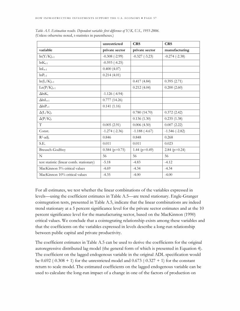
H O W I N F R A S T R U C T U R E I N V E S T M E N T S S U P P O R T T H E U . S . E C O N O M Y ■ P A G E 5 7
Table A.5. Estimation results. Dependent variable: first difference of Y/K, U.S., 1951-2006. (Unless otherwise noted, t-statistics in parentheses.)
unrestricted CRS CRS
variable private sector private sector manufacturing
ln(Y/K)t-1 -0.308 (-2.99) -0.327 (-3.23) -0.274 (-2.38) lnKt-1 -0.593 (-4.25) lnLt-1 0.400 (4.07) lnPt-1 0.214 (4.01) ln(L/K)t-1 0.417 (4.84) 0.395 (2.71) Ln(P/K)t-1 0.212 (4.04) 0.200 (2.60) ΔlnKt -1.126 (-4.94) ΔlnLt-1 0.777 (14.26) ΔlnPt-1 0.141 (1.16) Δ(L/K)t 0.780 (14.70) 0.372 (2.42) Δ(P/K)t 0.136 (1.30) 0.235 (1.38) T 0.005 (2.91) 0.006 (4.50) 0.007 (2.22) Const. -1.274 (-2.36) -1.188 (-4.67) -1.546 (-2.82) R2-adj. 0.846 0.848 0.268 S.E. 0.011 0.011 0.023 Breusch-Godfrey 0.584 (p=0.75) 1.44 (p=0.49) 2.84 (p=0.24) N 56 56 56 test statistic (linear comb. stationary) -5.18 -4.83 -4.12 MacKinnon 5% critical values -4.69 -4.34 -4.34 MacKinnon 10% critical values -4.35 -4.00 -4.00
For all estimates, we test whether the linear combinations of the variables expressed in levels—using the coefficient estimates in Table A.5—are trend stationary. Engle-Granger cointegration tests, presented in Table A.5, indicate that the linear combinations are indeed trend stationary at a 5 percent significance level for the private sector estimates and at the 10 percent significance level for the manufacturing sector, based on the MacKinnon (1990) critical values. We conclude that a cointegrating relationship exists among these variables and that the coefficients on the variables expressed in levels describe a long-run relationship between public capital and private productivity.
The coefficient estimates in Table A.5 can be used to derive the coefficients for the original autoregressive distributed lag model (the general form of which is presented in Equation 4). The coefficient on the lagged endogenous variable in the original ADL specification would be 0.692 (-0.308 + 1) for the unrestricted model and 0.673 (-0.327 + 1) for the constant return to scale model. The estimated coefficients on the lagged endogenous variable can be used to calculate the long-run impact of a change in one of the factors of production on

H O W I N F R A S T R U C T U R E I N V E S T M E N T S S U P P O R T T H E U . S . E C O N O M Y ■ P A G E 5 8
private capital productivity, taking into account the dynamic specification of the model. It is these long-run coefficient estimates which were used to produce Table 4 in the main text.
One concern with earlier studies of the impact of public capital on private productivity was that the implied rate of return on public investment, e.g. calculated from the estimates generated by Aschauer and Munnell, were implausibly high (for a discussion, see Munnell, 1992). However, these estimates did not take into account the fact that such effects would take many years to fully manifest themselves.
We estimate the implied rate of return on public investment using the coefficient estimates from Table A.5 and the dynamic specification of the model. In 2006, the stock of public capital, excluding educational buildings, hospitals, and conservation assets, was valued at $5.7 trillion and private sector GDP was estimated at $10.2 trillion, yielding an output/ infrastructure ratio of approximately 1.79. Multiplying this ratio by the long-run elasticity of output to public capital stock (0.214/0.308 = 0.695), which takes into account the dynamic impact on capital productivity implied by the coefficient on the lagged endogenous variable, gives us the estimate of the return to an additional $1 in infrastructure spending. A $1 increase in public capital should yield an additional $1.24 in private benefits in the long run. The coefficient estimate on the lagged endogenous variable implies that over 98 percent of this effect will be realized within 10 years of the initial investment. Calculating the average rate of return over 10 years yields an estimated annual return of approximately 8.3 percent, a credible return well below that implied in other studies.
E. Comparing Our Employment Estimates with those in the Obama Recovery Program
Christina Romer and Jared Bernstein’s paper “The Job Impact of the American Recovery and Reinvestment Act,” provides estimates of job creation that would result from a $775 billion economic stimulus program. Within the framework of their overall program, they estimate that the increase in employment associated with the infrastructure component of the program will be 377,000 jobs in total, including direct, indirect, and induced effects (they combine what we call indirect and induced effects into one category that they call “indirect).
This estimate is obviously substantially different than the estimates we have provided for two infrastructure investment programs:
A baseline program of $87 billion/year, that would generate 1.6 million jobs overall
A high-end program of $148 billion/year, that would generate 2.6 million jobs.
Why are there such large disparities between our respective employment estimates?
1. Romer/Bernstein do not specify in their paper how much new spending will be directed towards infrastructure investments. Until we know what their specific figure for infrastructure investment spending, we cannot draw comparisons between their figure and

H O W I N F R A S T R U C T U R E I N V E S T M E N T S S U P P O R T T H E U . S . E C O N O M Y ■ P A G E 5 9
ours. We can say this: within the framework of our model, we would generate 377,000 jobs through an infrastructure investment spending program on the order of $20 billion/year. We expect that the Obama program will allocate significantly more than $20 billion overall to infrastructure spending.
2. The Romer/Bernstein definition of “infrastructure” is likely to be different than the one we are using here. They also include separate categories for “energy” and “education” investment spending. Those categories likely incorporate school building construction and energy transmission systems, both of which are included in our definition of infrastructure investment.
3. The Romer/Bernstein modeling approach is different than ours. For generating employment effects, we have relied exclusively on a the simple input-output model approach that we describe above, based on the industrial survey data from the Department of Commerce, for the year 2006. This approach has both advantages and disadvantages—or to be more precise, its advantages are also its disadvantages. First, we are confident we are working with a reliable, if static, picture of the U.S. industrial structure as it exists today. Within that framework, our approach then asks a simple question: assuming the industrial structure stays the same, what is the impact on employment of increasing spending on infrastructure by a given amount, e.g. either $87 or $148 billion?
4. As such, the input-output model is incapable of discerning what might result if the industrial structure or broader economic circumstances change—for example, what would happen if interest rates rose due to the increased investment spending, or wages rose because labor market conditions began tightening? We are of course able to use the input-output model as a basis for trying to reason through how such considerations might play out. But these considerations do not come out naturally from the model.
5. It happens that the problems one faces in working with a static framework such as our input-output model become less significant when the economy is in a recession. This is because, in attempting to estimate the effects of an investment spending injection within a static model, the main factor that can lead to distorted results is that the increased investment spending creates supply constraints and price increases. For example, as mentioned above, in an economy operating at close to full capacity, an increase in infrastructure spending in the range of $87 - $148 billion could lead to rising interest rates and wages. These increases in interest rates and wages would produce higher business costs, which in turn could counteract the stimulative effects of the initial spending injection. But in our current circumstances, the effects of any possible supply constraints will be extremely weak. Thus, the reliability of a simple, static, input-output model increases when economic resources are slack. The reliability correspondingly declines when resources are tight—when we do not really know, for example, how we would find millions of more workers to construct $148 billion worth of new infrastructure. Under the present circumstances of

H O W I N F R A S T R U C T U R E I N V E S T M E N T S S U P P O R T T H E U . S . E C O N O M Y ■ P A G E 6 0
nearly 15 percent unemployment in construction, we know that these workers are available to take new employment opportunities.
6. The Romer/Bernstein paper is based on an unspecified combination of forecasting models. They do not present enough information to enable us to assess the quality and reliability of these models. The basic assumption used by Romer and Bernstein that employment will rise by 0.75 percent for every 1 percent increase in GDP is reasonable. But we do not know how they obtained their underlying GDP forecast. We also, again, do not know how the overall $775 billion spending program is distributed among infrastructure spending and other activities. Given the economic experiences of the past year and the prospects for the coming year, it is fair to say that forecasting GDP through any econometric model is a shaky proposition. It will be useful to recall a comment by then Federal Reserve Chair Alan Greenspan in 1999 on the reliability of the Federal Reserve’s own forecasting model: Greenspan said then that “The fact that our econometric models at the Fed, the best in the world, have been wrong for fourteen straight quarters does not mean that they will not be right in the fifteenth quarter.”
H O W I N F R A S T R U C T U R E I N V E S T M E N T S S U P P O R T T H E U . S . E C O N O M Y ■ P A G E 6 1
REFERENCES
Airport Council International (North America). 2007. Airport Capital Development Costs, 2007-2011. Washington, DC.
Aschauer, David A. 1989a. “Is public expenditure productive?” Journal of Monetary Economics 23(2): 177-200.
———. 1989b. “Does public capital crowd out private capital?” Journal of Monetary Economics 24(2): 171-188.
ASU (American School and University). Various years. Annual Official Education Construction Report.
American Society of Civil Engineers. 2005. Infrastructure Report Card 2005.
Army Corps of Engineers. 2005. The U.S. Waterway System: transportation facts. Navigation Data Center, Alexandria, VA.
Association of American Railroads. 2007. National Rail Freight Infrastructure Capacity and Investment Study. Washington, DC.
CRS (Congressional Research Service). 2008. Water Infrastructure Needs and Investment: Review and Analysis of Key Issues. Washington, DC.
Department of Energy. 2003. Grid 2030: a national vision for electricity’s second 100 years, Office of Electric Transmission and Distribution, Washington DC.
Department of Transportation. 2007. Transportation Statistics Annual Report. Washington, DC.
Department of Transportation, Federal Highway Administration and Federal Transit Administration. 2006. 2006 Status of the Nation’s Highways, Bridges, and Transit: Conditions and Performance. Washington, DC.
GAO (General Accountability Office). 2007. Airport finance: observations on planned airport development costs and funding levels and the administration’s proposed changes in the Airport Improvement Program. Washington, DC.
EIA (Energy Information Administration). 2008. Annual Energy Outlook 2008. Washington, DC.
EPA (Environmental Protection Agency). 2003. The Clean Water and Drinking Water Infrastructure Gap Analysis. Washington, DC.
FAA (Federal Aviation Administration). 2008. FAA Aerospace Forecasts Fiscal Years 2008-2025. Washington, DC.
Hemming, Richard, Kell, Michael, and Mahfouz, Selma. 2002. “The Effectiveness of Fiscal Policy in Stimulating Economic Activity: A Review of the Literature.” Washington, D.C.: International Monetary Fund.

H O W I N F R A S T R U C T U R E I N V E S T M E N T S S U P P O R T T H E U . S . E C O N O M Y ■ P A G E 6 2
Horowitz, Karen and Planting, Mark, “Concepts and Methods of the Input-Output Accounts,” Bureau of Economic Analysis, September 2006.
MacKinnon, J.G. 1990. “Critical values for cointegration tests.” Department of Economics Discussion Paper No. 90-4. University of California, San Diego.
Moreno, Rosina, Enrique López-Bazo, and Manuel Artís. 2002. “Public infrastructure and the performance of manufacturing industries: short- and long-run effects.” Regional Science and Urban Economics, 32: 97-121
Morrison, Catherine J. and Amy Ellen Schwartz. 1996. “State infrastructure and productive performance.” American Economic Review 86(5): 1095-111.
Munnell, Alicia H. 1990a. “Why has productivity growth declined? Productivity and public investment.” New England Economic Review Jan/Feb. 3-22.
———. 1990b. “How does public infrastructure affect regional economic performance?” New England Economic Review Sep/Oct. 11-32.
———. 1992. “Infrastructure investment and economic growth,” Journal of Economic Perspectives, 6(4): 189-98.
Nadiri, M. Ishaq and Theofanis P. Mamuneas. 1994. “The effects of public infrastructure and R&D capital on the cost structure and performance of U.S. manufacturing industries,” Review of Economics and Statistics 76(1): 22-37.
NCES (National Center for Education Statistics). 2000. Condition of America’s Public School Facilities: 1999. Washington, DC.
Pollin, Robert, Heidi Garrett-Peltier, James Heintz, and Helen Scharber. 2008. Green Recovery: A Program to Create Good Jobs and Start Building a Low-Carbon Economy, Center for American Progress and Political Economy Research Institute, http://www.peri.umass.edu/fileadmin/pdf/other_publication_types/peri_report.pdf
Romer, Christina and Jared Bernstein. 2009. “The Job Impact of the American Recovery and Reinvestment Plan,” http://otrans.3cdn.net/45593e8ecbd339d074_l3m6bt1te.pdf
Sturm, Jan Egbert and Jakob de Haan. 1995. “Is public expenditure really productive? New evidence for the U.S. and the Netherlands.” Economic Modelling 12(1): 60-72.
Tatom, J.A. 1991. “Public capital and private sector performance.” Federal Reserve Bank of St. Louis Review 73(3): 3 -15.
Tobin, James. 2008. “Major changes in natural gas transportation capacity, 1998-2008” Presentation (Powerpoint). Office of Oil and Gas, Energy Information Administration, Washington, DC.

About AAMThe Alliance for American Manufacturing (AAM) is a unique non-partisan, non-profit partnership forged to strengthen manufacturing in the U.S. AAM brings together a select group of America’s leading manufacturers and the United Steelworkers. Our mission is to promote creative policy solutions on priorities such as international trade, energy security, health care, retirement security, currency manipulation, and other issues of mutual concern.
ContactAlliance for American Manufacturing
727 Fifteenth Street, NW, Suite 700 Washington, DC 20005phone: 202-393-3430 fax : 202-628-1864 email: [email protected]
www.americanmanufacturing.org
About PERIThe Political Economy Research Institute (PERI) promotes human and ecological well-being through our original research. Our approach is to translate what we learn into workable policy proposals that are capable of improving life on our planet today and in the future. In the words of the late Professor Robert Heilbroner, we at PERI “strive to make a workable science out of morality.” Established in 1998, PERI is an independent unit of the University of Massachusetts, Amherst, with close ties to the Department of Economics. Since its founding, PERI has become a leading source of research and policy initiatives on issues of globalization, unemployment, financial market instability, central bank policy, living wages and decent work, and the economics of peace, development, and the environment.
ContactPolitical Economy Research Institute (PERI)
University of Massachusetts-Amherst, Gordon Hall 418 N. Pleasant St., Suite A, Amherst, MA 01002
Phone: 413-545-6355 Fax: 413-577-0261General inquiries: [email protected]