Embed Size (px)
Citation preview

NBER WORKING PAPER SERIES
HOW ELASTIC ARE PREFERENCES FOR REDISTRIBUTION? EVIDENCE FROMRANDOMIZED SURVEY EXPERIMENTS
Ilyana KuziemkoMichael I. NortonEmmanuel Saez
Stefanie Stantcheva
Working Paper 18865http://www.nber.org/papers/w18865
NATIONAL BUREAU OF ECONOMIC RESEARCH1050 Massachusetts Avenue
Cambridge, MA 02138March 2013
We thank co-editor Marianne Bertrand, Raj Chetty, Amy Finkelstein, Ray Fisman, Lawrence Katz,Wojciech Kopczuk, James Poterba, Andrea Prat, Jonah Rockoff, four anonymous referees, and numerousseminar and conference participants for helpful comments and discussions. Pauline Leung providedoutstanding research assistance. Financial support from the Center for Equitable Growth at UC Berkeley,the MacArthur Foundation, and NSF Grant SES-1156240 is gratefully acknowledged. The views expressedherein are those of the authors and do not necessarily reflect the views of the National Bureau of EconomicResearch.
NBER working papers are circulated for discussion and comment purposes. They have not been peer-reviewed or been subject to the review by the NBER Board of Directors that accompanies officialNBER publications.
© 2013 by Ilyana Kuziemko, Michael I. Norton, Emmanuel Saez, and Stefanie Stantcheva. All rightsreserved. Short sections of text, not to exceed two paragraphs, may be quoted without explicit permissionprovided that full credit, including © notice, is given to the source.
How Elastic Are Preferences for Redistribution? Evidence from Randomized Survey ExperimentsIlyana Kuziemko, Michael I. Norton, Emmanuel Saez, and Stefanie StantchevaNBER Working Paper No. 18865March 2013, Revised June 2014JEL No. D63,D72,H2,I3
ABSTRACT
We develop online survey experiments to analyze how information about inequality and taxes affectspreferences for redistribution. Approximately 4,000 respondents were randomized into treatmentsproviding interactive, customized information on U.S. income inequality, the link between top incometax rates and economic growth, and the estate tax. An additional 6,000 respondents were randomizedinto follow-up treatments to explore mechanisms underlying the initial results. The treatment has verylarge effects on whether respondents view inequality as a problem. By contrast, it only slightly movespolicy preferences (e.g., top income tax rates and transfer programs). An exception is the estate tax—informingrespondents of the small share of decedents who pay it more than doubles support for it and this effectpersists in a one-month follow-up. We explore several explanations for our results. Extreme ex-antemisinformation appears to drive the large estate tax results. The small effects for all other policiescan be at least partially explained by respondents' low trust in government—indeed, we show thatpriming people to think negatively about the government substantially reduces support for transferprograms—as well as a disconnect between concerns about social issues and the public policies thataim to address them.
Ilyana KuziemkoColumbia UniversityGraduate School of Business3022 BroadwayUris HallNew York, NY 10027and [email protected]
Michael I. NortonMarketing UnitHarvard Business SchoolBoston, MA [email protected]
Emmanuel SaezDepartment of EconomicsUniversity of California, Berkeley530 Evans Hall #3880Berkeley, CA 94720and [email protected]
Stefanie StantchevaMIT Department of Economics50 Memorial DriveBuilding E52Cambridge, MA [email protected]
1 Introduction
Over the past several decades, there has been a large increase in income concentration in the
United States. While the top one percent of families captured 9.0 percent of total pre-tax
income in 1970, that share rose to 22.4 percent by 2012.1 More recent work has documented
a corresponding trend for wealth concentration: the top 0.1 percent share of wealth has
grown from 8 percent in the mid-1970s to 22 percent in 2012.2 These trends have not gone
unnoticed, at least by some. The Occupy Wall Street movement popularized the term “the
one percent.” Recently, President Obama has called “a dangerous and growing inequality”
the “defining challenge of our time,” a sentiment echoed by the CEO of Goldman Sachs,
who told an interviewer that “too much of the GDP of the country has gone to too few of
the people.”3
The standard political economy model suggests that tax and transfer policy will react
to rising market income inequality. Specifically, the median-voter theorem predicts that an
increase in the demand for redistribution—and thus an increase in top tax rates, as politicians
respond to voters’ wishes—should accompany this rise in income concentration (Meltzer and
Richard, 1981).4 By contrast, top income tax rates as well as inheritance tax rates have fallen
in the United States during this period.5 While for institutional reasons the policy views of
the majority might be ignored by policy-makers (Bartels, 2009), even more challenging to
the model’s predictions is that survey respondents themselves show no increased demand
for redistribution during this period.6 If anything, the General Social Survey shows there
has been a slight decrease in stated support for redistribution in the United States since
the 1970s, even among those who self-identify as having below-average income (see Figure
1). These trends have led commenters to suggest that Americans simply do not care about
1See the online updates to Piketty and Saez (2003), Table A3 athttp://elsa.berkeley.edu/~saez/TabFig2012prel.xls
2See http://gabriel-zucman.eu/files/SaezZucman2014Slides.pdf.3See http://www.whitehouse.gov/the-press-office/2013/12/04/remarks-president-
economic-mobility and http://thinkprogress.org/economy/2014/06/13/3448679/goldman-
sachs-income-inequality/, respectively.4Note that the self-interested voter might not be a good model of policy preferences. After all,
self-interested individuals would not vote in the first place if voting is privately costly.5For top income tax rates, see Piketty, Saez, and Stantcheva (2014) and for estate taxes see IRS
calculations at http://www.irs.gov/pub/irs-soi/ninetyestate.pdf.6See, e.g., Kenworthy and McCall (2008), for evidence from a variety of OECD countries that
saw increases in inequality but no corresponding increase in redistributive demand.
1

rising inequality.7
There are alternative explanations: Americans may be unaware of the extent or growth of
inequality (see Kluegel and Smith, 1986 and Norton and Ariely, 2011), this information may
not be sufficiently salient, or they are skeptical about the government’s ability to redistribute
effectively. In this paper, we extensively examine these explanations. We conduct a series
of randomized survey experiments using Amazon’s Mechanical Turk (mTurk). mTurk is a
rapidly growing online platform that can be used to carry out social and survey experiments
(see Horton, Rand, and Zeckhauser, 2011 and Paolacci, Chandler, and Ipeirotis, 2010). In our
initial set of experiments, comprising just over 4,000 respondents, half of respondents were
randomized into an “omnibus” treatment providing interactive, personalized information on
U.S. income inequality, the historical correlation between top income tax rates and economic
growth, and the incidence of the estate tax. Both control and treatment groups then reported
their views on inequality, redistributive policies, and government more generally. We then
conducted follow-up experiments with about 6,000 new respondents to analyze potential
mechanisms behind the initial results, for a total of approximately 10,000 respondents.8
Our treatments exploit the flexibility of the mTurk platform to include several features
that heighten the salience of the information we present. First, some of the information we
present is customized. For example, we ask individuals their household income, allowing us
to show them their place in the income distribution, as well as their counterfactual income
level had aggregate income growth since 1980 been distributed more equally (so as to leave
inequality unchanged). In other parts of the survey, we customize information based on
respondents’ own household composition.9 Second, some of the information is interactive—
for example, our survey allows respondents to enter different household income levels and
the software survey application provides the corresponding percentile, so that the income
distribution can be transparently explored.
The initial survey experiment provides several findings we believe to be novel relative to
existing literature; the first part of the paper provides a descriptive analysis of these results.
First, we find that respondents’ concern about inequality is very elastic to information—
7As Newsweek put it in 2001: “If Americans couldn’t abide rising inequality, we’d now bedemonstrating in the streets.”
8Survey questions and treatments are all available online athttps://hbs.qualtrics.com/SE/?SID=SV_77fSvTy12ZSBihn.
9Recent work has highlighted the potential power of customizing information in interventions.For example, Hoxby and Turner (2013) credit the customized nature of the information they presentto students for the large effects their intervention had on college application decisions.
2

for example, the treatment increases the share agreeing that inequality is a “very serious
problem” by over 35 percent. Put differently, the treatment effect is equal to roughly 36
percent of the gap between self-identified liberals and self-identified conservatives on this
question. By contrast, while there are some effects on policy preferences such as top income
tax rates, the minimum wage and food stamps (always in the “expected” direction), they
are small and often insignificant despite the large sample size.
The only exception is the estate tax—we find that providing information on the (small)
share of estates subject to the tax more than doubles respondents’ support for increasing it.
Focusing on the estate tax result, we attempt to make progress on two long-standing critiques
about survey analysis: that the effects are ephemeral and unrelated to actual behavior. We
benefit from the mTurk technology and re-survey respondents one month later: the estate
tax effect is virtually unchanged. We also find that the treatment significantly increases the
share of respondents who say they would send a petition to one of the U.S. Senators from
their state to raise the estate tax.
The second half of the paper explores the mechanisms behind the large estate-tax effects
and the muted response for any other policy outcome. Of course, other explanations may
exist and as such we do not view our attempts to tease out the mechanisms behind the main
results as definitive.
Consistent with past work, we find that respondents are wildly misinformed about the
share of decedents subject to the estate tax, which appears to account for the large effects. We
further show that the estate tax effect remains strong even when we take steps to decrease
the salience and emotional content of the information provided, further proof that basic
information on this issue has large effects.
We test three potential explanations for the small effects for other policies: limited trust
in government; an overly “clinical” presentation of information; and respondents’ inability
to connect their concerns on a given issue with the public policies meant to address it.
The first potential explanation is that distrust in government inhibits respondents from
translating concern for inequality into support for redistribution by the government. Several
results from the original survey experiment point in this direction. First, our initial treat-
ment significantly decreases trust in government. When reminded of the extent of inequality
(which even control group respondents view as a problem), those in the treatment group
appear to at least partially blame the government, perhaps thinking that if politicians “let
things get this bad” they cannot be trusted. Second, beyond any treatment effect, the level
3
of government trust among our sample of mTurk respondents are very low: over 89 percent
agree that “Politicians in Washington work to enrich themselves and their largest campaign
contributors, instead of working for the benefit of the majority of citizens,” with 47 per-
cent “strongly” agreeing. It is thus perhaps not surprising that even when the treatment
increases respondents’ concern with inequality, they remain reluctant to increase support for
government redistributive policies.
In a follow-up survey experiment, we provide direct evidence for the effect of trust in
government on respondents’ policy preferences. We first asked a small pilot group to an-
swer open-ended questions on their views of government—the main theme that emerges is
that politicians are believed to work to enrich themselves and their wealthiest campaign
donors. We then used these answers to develop primes (e.g., asking respondents’ opinions
about lobbyists or the Wall Street bailout) that significantly lowered trust in government
without significantly changing views about the extent of inequality or poverty. Therefore,
the treatment isolates the causal effect of decreasing trust in government. We find that the
treatment significantly lowers support for all poverty-alleviation policies, with the exception,
interestingly, of the minimum wage—a program that does not involve direct transfers from
the government. Support for top tax rates generally falls as well (though only some of these
effects are significant) and respondents elevate “private charity” over government policies
in a list of the best ways to combat inequality. To the best of our knowledge, this analysis
provides the first evidence on the casual effects of trust in government on policy preferences,
and is particularly relevant given the historically low regard with which Americans currently
view their government.10
Besides distrust muting the policy effects of our treatment, we explore two other potential
explanations for the small results in the original survey experiment. As Brader (2005) and
others argue, policy preferences might respond more to emotional than factual appeals. We
thus develop a treatment—again, interactive and customized—designed to evoke empathy for
households at the poverty line. Just as in the initial survey experiment, the treatment signifi-
cantly increases respondents’ tendency to view inequality and poverty as “serious problems”
but has almost no effect on policy preferences.
We find more support for a third explanation, the idea in Bartels (2005) that the public
fails to connect concern for inequality with actual public policy measures. To test this idea,
10See analysis from Gallup: http://www.gallup.com/poll/164663/americans-trust-
government-generally-down-year.aspx. The General Social Survey also shows a stronglynegative trend.
4

we repeat much of the information in the “emotional appeal” treatment, but then show re-
spondents concretely the resources provided to such families through government programs
including the minimum wage and food stamps. Therefore, the treatment directly connects
poverty and inequality with policies meant to address them. Emphasizing this connection
appears important: treatment respondents significantly increase their support for the min-
imum wage as well as most of the poverty-alleviation programs that we survey. We view
this result as potentially complementary to the trust results: given the low baseline levels of
trust, it appears to be the case that policy preferences can only be moved if respondents are
explicitly reminded of efficacious examples of government activity.
We believe our findings make several contributions to the understanding of how individ-
uals form—and change—their redistributive preferences. Compared to most informational
interventions that merely provide a fixed set of facts to respondents, our informational treat-
ments were interactive and customized—while perhaps not providing a strict upper bound
on the effects of information on preferences, our results do suggest that most policy prefer-
ences are hard to move. This finding echoes Luttmer and Singhal (2011) that redistributive
preferences may have “cultural” determinants that are very stable over time.
Our results also highlight the potential role of mistrust of government in limiting the
public’s enthusiasm for policies they would otherwise appear to support, a subject that has
garnered limited attention in the economics literature. An exception is Sapienza and Zingales
(2013), who find that a major reason respondents support auto fuel standards over a gasoline-
tax-and-rebate scheme is not because they misunderstand the incidence of fuel standards but
because they simply do not trust the government to actually rebate them their money.
More generally, our paper relates to the literature on the determinants of redistributive
preferences, to which political scientists, sociologists, psychologists and public economists
have all contributed. Many papers in this literature use survey data to relate individual
traits to redistributive preferences and do not, as we do, take an experimental approach.
Alesina and Ferrara (2005), Alesina and Giuliano (2011), and Fong (2001) show that, re-
spectively, prospects for future income mobility, past experience of misfortune, and beliefs
about equality of opportunity predict redistributive preferences. Other papers have exam-
ined how situational factors (employment status, neighborhood characteristics) predict pref-
erences (see, e.g., Margalit 2013, Luttmer 2001). Singhal (2008) uses OECD survey data
to show that people do not necessarily favor low tax rates at income levels close to theirs,
suggesting that redistributive preferences are not completely determined by self-interest.
5

As in our paper, some researchers have estimated the effects of randomized informational
treatments on policy preferences.11 The evidence from these efforts is mixed. Sides (2011)
finds that providing information on the very small number of individuals affected by the
estate tax drastically decreases support for its repeal, results that we replicate with our data.
Cruces, Perez-Truglia, and Tetaz (2013) find that showing poor individuals their actual place
in the income distribution increases their support for policies that target poverty, as most
overestimate their income. On the other hand, Kuklinski et al. (2003) find that providing
(accurate) information on the demographic composition of welfare recipients and the share of
the federal budget dedicated to welfare payments has no effect on respondents’ preferences,
despite the fact that their initial beliefs are wildly incorrect.12 We examine a wide variety
of redistributive policy outcomes; indeed, we find that the responsiveness of views on the
estate tax appears to be an outlier and other outcomes suggest a far more modest effect of
information on redistributive preferences.
As noted, our research is part of a small but growing set of papers using online platforms.
Researchers have used these platforms—most often, mTurk—to have respondents play public
goods games (e.g., Rand and Nowak, 2011, Suri and Watts, 2010), interact in online labor
markets (Amir, Rand, and Gal 2012; Horton, Rand, and Zeckhauser 2011), or simply answer
non-experimental survey questions on views about policy and social preferences (Weinzierl
2012; Saez and Stantcheva 2013). We summarize our experience conducting survey exper-
iments on mTurk in the online Methodological Appendix, which we hope can be of use to
future researchers utilizing this platform.
The paper proceeds as follows. Section 2 introduces the initial survey instrument and
data collection procedures. Section 3 describes the data. Section 4 presents the main results
of the survey experiment. In Section 5, we explore mechanisms behind the large effects
of information on views about the estate tax and why most other effects were so limited,
reporting methods and results from four follow-up survey experiments. Finally, in Section 6,
we suggest directions for future work and offer concluding thoughts.
11While not related to policy preferences, there is a small literature on how information treatmentsaffect individuals’ ability to better navigate policies such as Social Security (Liebman and Luttmer,2011).
12Related but distinct from informational treatments are priming and presentational treatments(see, e.g., Savani and Rattan 2012 on the effect of priming about free-will and McCaffery and Baron2006 on the effects of presenting taxes in absolute or percentage terms).
6

2 The Main Survey Experiment
The main experiment was implemented in four separate rounds from January 2011 to August
2012. For expositional clarity, to distinguish this initial experiment from the follow-up work
we describe in Section 5, we refer to these four initial rounds of surveys as the “omnibus”
treatment surveys.
The omnibus treatment surveys had the following structure: (1) background socio-economic
questions including typical demographic questions as well as political leanings; (2) random-
ized treatment providing information on inequality and tax policy (shown solely to the treat-
ment group); (3) questions on views on inequality, tax and transfer policies, and government
more generally.13
2.1 Data collection
Surveys were openly posted on mTurk with a description stating that the survey paid $1.50
for approximately 15 minutes, i.e., a $6 hourly wage. Respondents were free to drop out any
time or take up to one hour to answer all questions. As a comparison, the average effective
wage on mTurk according to Amazon is around $4.80 per hour and most tasks on mTurk
are short (less than one hour).14
Several steps were taken to ensure the validity of the results. First, there are many
foreign workers on mTurk, especially from Asia. In addition to requiring respondents to
confirm their U.S. residency on the consent form, we also had Amazon show the survey only
to workers who had U.S. addresses. Second, to further discourage foreign workers, we tried
to launch our surveys during East Coast daylight hours (and, to reduce heterogeneity, only
on workdays). Third, only workers with a past completion rate of at least ninety percent
were allowed to take the survey, in order to exclude robots. Fourth, as our survey comprises
many rounds, we block workers who had participated in a previous round of the survey.
Fifth, respondents were told that payment would be contingent on completing the survey
13The Appendix provides a complete description of the experiment with the questions for eachround of the main experiments, as well as the follow-up experimental rounds that we describe laterin the paper.
14In order to gauge the generalizable of results on mTurk to results on other platforms, wegathered data for round 3 using C&T Marketing (http://www.ctmarketinggroup.com/). As notedin Section 4, effects are stable across rounds, suggesting that respondents from the two platformsrespond similarly to the treatment. See the Methodological Appendix for more detail. Note thatper-participants costs for C&T are roughly five times higher than for mTurk.
7

and providing a password visible only at completion. Finally, to discourage respondents from
skipping mindlessly through the pages, pop-up windows with an encouragement to answer
all questions appeared as prompts whenever a question was left blank.
2.2 The omnibus information treatment
In general, the goal of the information treatments was to provide a large “shock” to indi-
viduals’ information about inequality and redistributive policies, rather than to provide a
Ph.D-level, nuanced discussion about, say, the underlying causes of inequality or the trade-off
between equality and efficiency. Hence, some of the treatments we display will seem overly
simplified to an economics audience, but it should be kept in mind that our goal in the initial
experiment is to test whether any treatment can move redistributive preferences; thus we
erred on the side of presenting information we thought would indeed move those preferences.
As noted in the introduction, we took steps to make the information both interactive and
customized to each respondent.
The treatment had three basic parts. First, treatment respondents saw interactive infor-
mation on the current income distribution—they were asked to input their household income
and were then told what share of households made more or less than their household. We
also asked them to find particular points in the distribution—they were asked to find the
median and the 90th and 99th percentiles and were encouraged to “play around” with the
application. Appendix Figure 1 presents a screen shot.15
The second part focused not on the current distribution but a counterfactual: respon-
dents entered their current income and were then shown what they “would have made” had
economic growth since 1980 had been evenly shared across the income distribution (i.e., had
the level of inequality stayed the same as in 1980). Of course, this exercise abstracts away
from the trade-off between efficiency (economic growth) and equality that would certainly
exist at very high levels of taxation. The interactive application allowed them to find this
counterfactual value for any point of the current income distribution. Appendix Figure 2
presents a screen shot.
15As detailed in Appendix Table 1 we also ask treatment respondents six “basic comprehension”questions to determine if the information was confusing. With one exception, each question exhibitsat least eighty percent comprehension. Moreover, more than 74 percent of respondents answer atleast five of the six questions correctly. There are no differential treatment effects by comprehensionlevel (results available upon request), not surprising given that comprehension is at a fairly high(and uniform) level.
8
The third part of the treatment focused on redistributive policies. To emphasize that
higher income taxes on the well-off need not always lead to slower economic growth, we
presented respondents a figure showing that, at least as a raw correlation, economic growth,
measured by average real pre-tax income per family from tax return data, has been slower
during periods with low top tax rates (1913 to 1933 and 1980 to 2010) than with high top tax
rates (1933 to 1980). Appendix Figure 3 presents a screen shot. Similarly, we also presented
a slide on the estate tax, emphasizing that it currently only affects the largest 0.1 percent of
estates. Appendix Figure 4 presents a screen shot.
Readers can directly experience these informational treatments online at the link below.16
We describe the additional treatments in the follow-up surveys in Section 5.
3 Data
3.1 Summary statistics
Table 1 shows characteristics of the sample who completed the omnibus treatment survey
rounds (we discuss attrition below). We compare these summary statistics to a nationally
representative sample of U.S. adults contacted by a CBS poll in 2011, which we choose
both because it was conducted around the same time as our surveys and asks very similar
questions.17 We also compare it to a more representative (though far more expensive) online
panel survey gathered by RAND, the American Life Panel.18
Our sample is younger, more educated and has fewer minorities. It is more liberal, with
a higher fraction reporting having supported President Obama in the 2008 election.19
16See https://hbs.qualtrics.com/SE/?SID=SV_77fSvTy12ZSBihn. Note that the controlgroup went straight from the background questions to the outcomes measures (starting with thepreferred tax rates sliders).
17Note that the CBS sample is not as representative as the traditional surveys used by economistssuch as the Current Population Survey or the American Community Survey. However, these twosurveys do not have questions on past voting behavior or political preferences, so we rely on theadmittedly less representative CBS survey.
18The American Life Panel currently costs researchers $3 per subject per minute, compared toroughly $.10 per subject per minute for our mTurk surveys. The ALP survey is also limited insample size.
19As a robustness check, we created weights to match our mTurk sample in col. (1) to the CBSpoll in col. (2) with respect to the 32 cells based on: gender (2) × age brackets (2) × white versusnon-white (2) × college degree indicator (2) × Supported Obama in 2008 (2). Reweighting has noappreciable effects on the results in Tables 4 and 5 (results available upon request) and thus wefocus on the unweighted results in the paper.
9

Table 2 shows summary statistics on demographic and policy views for self-reported
liberals (col. 1) and conservatives (col. 2) from our control group (so that responses are not
contaminated by the information treatment), as well as the entire control group (col. 3). As
expected, conservatives are older, more white, and more likely to be married. They prefer
lower taxes on the rich and a less generous safety net. Such contrasts are useful to scale
the magnitude of our effects. We will often discuss treatment effects both in absolute terms
and as a percentage of the liberal-versus-conservative differences reported in Table 2. For
convenience, we refer to this difference as the “political gap” for a given outcome variable.
3.2 Survey attrition
The omnibus survey experiment had an overall attrition rate of 22 percent, which includes
those who attritted as early as the consent page. For those who remained online long enough
to be assigned a treatment status, attrition was 15 percent.
As Appendix Table 2 shows, attrition is not random, though it is unrelated to 2008 voting
preferences and liberal versus conservative policy views (the variables most highly correlated
with our outcome variables). The online survey for the treatment group was, by necessity,
different from the online survey for control group. Therefore, a key concern is differential
attrition between those assigned to the treatment versus control arms. As the final row of
Table 2 shows, attrition is higher among the treatment group (twenty percent, versus nine
percent for the control group).20
Importantly, however, conditional on finishing the survey, assignment to treatment ap-
pears randomly assigned. That is, while the treatment induces attrition, it does not induce
certain groups to differentially quit the survey more than others. Table 3 shows the results
from estimating (using the sample who complete the survey) 14 separate regressions of the
form: Treatmentir = βCovariateir + δr + εir, where i indexes the individual, r the sur-
vey rounds, and δr are survey-round fixed effects.21 For each regression, one of the control
variables in Table 2 serves as Covariate. Of the 14 regressions, only two (for the black
and Hispanic indicators) yield significant coefficients on the Covariate variable. However,
20For this comparison, we can obviously only include individuals who remained in the surveylong enough to have been assigned a treatment status. The other comparisons in this table includeall those who remained long enough to answer the given covariate question.
21We include round fixed effects δr because in one round we assigned more than half the respon-dents to the treatment. As such, without round fixed effects, Treatment becomes mechanicallycorrelated to the characteristics of respondents in this round.
10

given that their point-estimates have opposite signs, it does not seem that, say, minorities
systematically attrit from the sample if they are assigned to the treatment.
While we will control for these covariates as well as perform additional checks of attrition
in the analysis that follows, it is reassuring to see that, conditional on finishing the survey,
there does not appear to be a discernible pattern in the types of respondents assigned to
treatment. We are quite fortunate in this regard, as one might have expected that groups
pre-disposed against reading about inequality—perhaps conservatives or wealthier people—
would have been “turned off” by the treatment and differentially attired. Note also that
the follow-up surveys discussed in Sections 5 have essentially zero differential attrition by
treatment status (see Appendix Table 3), most likely because the treatments in the follow-up
surveys are much shorter (making the treatment and control arms of the survey much closer
in length).
4 Results from the omnibus treatment
We present three sets of results. Our first set of results captures how the treatment affects
respondents’ answers to questions related to inequality per se, not policies that might affect
it. Our second set of results relate to specific policies—e.g., raising taxes or increasing the
minimum wage. Our final set of results relate to views about government and respondents’
political involvement.
4.1 Views on inequality
Table 4 presents the effect of the omnibus treatment on questions related to inequality and
income distribution. Odd-numbered columns do not include any controls outside of round
fixed effects, while even-number columns include standard controls (essentially, those listed
in Table 3).22
Col. (1) shows that the treatment is associated with a ten-percentage-point (or 36 percent)
increase in the share agreeing that inequality is a “very serious” problem. Similarly, dividing
the point-estimate by the ‘political gap’ (i.e., the liberal-conservative control group difference
for the outcome variable) suggests that the treatment effect is equal to 36 percent of the
22Specifically, we include fixed effects for racial/ethnic categories, employment status, and stateof residence; indicator variables for voting for Barack Obama in 2008, being married, gender,and native-born status; continuous controls for age; and categorical variables for the liberal-to-conservative self-rating, household income, and education.
11
political gap on this question (which, as Table 2 shows, is 38 percentage points). While a
convenient scaling, dividing by the political gap is hardly a perfect metric—while political
views are highly predictive of many of our outcomes, this tendency varies and therefore
some questions have larger political gaps than others. We thus report both the absolute and
scaled effects for all regressions. Adding covariates in col. (2) has no effect on the estimated
treatment effect.
The effects on the outcome “did inequality increase since 1980?” are presented in columns
(3) and (4) and are even larger both in absolute percentage points and when scaled by the po-
litical gap (54 percent of the conservative-liberal difference), likely because the informational
treatment presented information directly related to the question.
The effects on respondents’ opinion of whether the rich are deserving of their income
are presented in column (5). They are statistically significant, but markedly smaller in
magnitude—equal to about five percentage points, or one-sixth the political gap. There-
fore, it does not seem that treatment respondents’ concern about inequality is being driven
primarily by a vilification of the rich.
In no case does the choice to exclude or include controls change the results (consistent with
the results from Table 3 that conditional on finishing the survey, there was little correlation
between treatment status and standard covariates). Therefore, to conserve space and reduce
noise, we show all results with covariates in the rest of the analysis.
Overall, our omnibus treatment generated a very strong “first stage,” significantly shifting
views about inequality and its increase in recent decades.
4.2 Views on public policy
Table 5 presents results for questions related to income and estate taxation. The first two
columns report results from the two questions on income taxation—a continuous variable
asking respondents to choose an ideal average tax rate for the richest one percent and a
categorical variable asking them whether taxes on millionaires should be raised—show sta-
tistically significant effects of the treatment, in the “expected” direction.23 However, these
magnitudes are small, equal to about ten percent of the liberal-conservative gap in both
cases. For example, the treatment increases the preferred top 1% average tax rate by 0.93
percentage points, whereas the gap between liberals and conservatives on this question is
slightly over ten percentage points (see Table 2). The omnibus treatment was hardly subtle
23See Appendix Figure 5 for the screen respondents used to choose their ideal tax rates.
12
in its discussion of income taxes, focusing on how income growth might be shared more
equitably through higher taxation and illustrating the temporal correlation between periods
of high top tax rate and strong economic growth. We also asked the income tax question
in two different ways, so the small magnitude of the results is unlikely to be an artifact of
framing.
By contrast, there are very large effects for the estate tax (col. 3), consistent with Sides
(2011). The treatment triples the share of respondents reporting a desired increase in the
estate tax, and the effect size is more than double the liberal-conservative gap on this ques-
tion.
A common critique of survey experiments that find large effects on opinion is that one
cannot know how these effects impact actual behavior. We try to partially bridge this gap
by asking individuals whether they would send a petition to their U.S. Senator asking either
to raise or lower the estate tax. We provided a link to Senators’ emails and also provided
sample messages both for and against raising estate taxes. We then asked if the respondent
would send a petition for higher taxes, would send a petition against higher taxes, or would
do nothing at all.
We report these results in col. (4). The treatment significantly increases the propensity
of respondents to say they would petition their U.S. Senator to raise the estate tax (though,
not surprisingly, this effect is smaller than the pure opinion question, suggesting attenuation
from belief to action). Naturally, we recognize that we must take respondents’ word that they
will send the email and thus this outcome is not as concrete as, for example, knowing with
certainty how they would vote in the next election. At the very least, this result confirms
the strong effect of the treatment on views about the estate tax. In Section 5, we probe the
robustness of this result and offer some thoughts on why it is so different from the income
tax. For now we merely note that these large results serve to dismiss a potential explanation
of why the income tax results were so small—that there is something inherent in the mTurk
experience that mutes respondents’ policy responses.
While so far we have focused on policies that affect the well-off, we also asked a series
of questions about policies that impact the bottom of the income distribution. While the
treatment induces significant but small (less than ten percent of the political gap) effects for
the minimum wage (col. 5), it induces no significant increase in support for food stamps or
the Earned Income Tax Credit (EITC) (cols. 6 and 7).24 The results thus suggest a contrast
24In later follow-up work, we asked a small pilot group to write open-ended responses to many of
13
between direct transfer policies such as the EITC and food stamps and indirect transfer
policies such as the minimum wage, a theme that will also emerge in some of the follow-up
work discussed in next section.25
4.3 Views of government and political involvement
Columns (8)-(10) of Table 5 reports results on the effect of the treatment on opinions about
government. The first question asked respondents: “How much of the time do you think
you can trust government in Washington to do what is right?” and we code a respondent
as trusting government if she answers “always” or “most of the time” as opposed to “only
some of the time” and “never.”26 Col. (8) reports a large decrease in the share of treatment
respondents agreeing that the government can be trusted. The treatment is equal to the
entire liberal-conservative gap, but operates in the opposite direction to the other outcomes,
in that it makes respondents take the more conservative—and less trusting—view on this
question.27 Note also that, consistent with the trends noted in the Introduction, the control
group has a very low level of trust in government—only about 16 percent are trusting of
government, by our definition—and that the contrast of liberals and conservatives about
trusting government is fairly small (17% vs. 14.5%, see Table 2). The low baseline level
of trust in the control group suggests that the treatment effect we observe might in fact
understate the true effect experienced by the treatment group, as their ability to express an
even lower opinion of government is limited by floor effects.
The second question assesses respondents’ preferred scope of government: “Next, think
more broadly about the purpose of government. Where would you rate yourself on a scale
of 1 to 5, where 1 means you think the government should do only those things necessary to
provide the most basic government functions, and 5 means you think the government should
take active steps in every area it can to try and improve the lives of its citizens?” Intriguingly,
our outcome variables. Many respondents had little familiarity with the EITC (though we alwaysprovided a description) so the non-result for that outcome might need to be interpreted morecautiously. No respondent indicated unfamiliarity with food stamps or the minimum wage, however.
25There are other possible distinctions between these policies. For example, respondents mayhave stronger racial stereotypes of food-stamp recipients than they do of minimum-wage workers.
26These questions were taken from Gallup.27We say that being less trusting of government is the “conservative” view because in our data as
well as GSS data from the same time period, conservatives indeed report lower trust in government.However, these tendencies are very sensitive to the party in power (e.g., in the GSS, during theGeorge W. Bush administration, self-described conservatives were more trusting of the executivebranch than were liberals).
14

the treatment significantly moves people toward wanting a more active government (col. 9).
Providing information about the growth of inequality and the ability of the government to
raise taxes and redistribute have complicated effects on views of government. It appears to
make respondents see more areas of society where government intervention may be needed
but simultaneously make them trust government less. We return to these results linking trust
in government to preferences on government scope in Section 5.2.1.
Finally, as shown in col. (10), the treatment has almost no effect on respondents’ planned
voting choice for the 2012 Presidential elections (recall that the omnibus-treatment surveys
were completed before the November 2012 election). There is at best a marginal effect in
the direction of supporting President Obama. This result is consistent with the relatively
mild policy effects overall. The treatment may simultaneously make individuals want the
more redistributive policies of the Democratic party and distrust the party in power (the
Democrats under Obama, at least in the executive branch and the Senate).28
4.4 Robustness checks
Persistence of effects. Before mTurk, recontacting survey respondents was onerous, and
thus few papers were able to test the duration of effects from informational survey exper-
iments. None of the papers cited in the Introduction on the effect of information on redis-
tributive preferences follows up with respondents to measure the duration of the effects.29
The evidence from the few papers that do test persistence is not encouraging. Luskin,
Fishkin, and Jowell (2002) find that even the immediate effects of an extreme intervention—
in which British participants spent a weekend with experts with the goal of debunking
misconceptions about crime and prison policy—do not persist ten months later. Indeed, in a
similarly intense intervention focused on issues related to campaign finance, Druckman and
Nelson (2003) find that their results dissipate within ten days. While not a survey experiment
per se, Gerber et al. (2011) use variation in the location of campaign television advertising to
show that persuasive effects are strong the week the ad airs but has little persistence beyond
the first week. Perhaps closest to our methodology, Lecheler and Vreese (2011) sample Dutch
respondents to test for the effect of informational treatments on opinions about economic
28In the interest of space, there are some outcome variables we relegate to the Appendix. Thefull set of all results from the omnibus survey are found in Appendix Tables 4 and 5.
29In their review of the use of survey experiments, Gaines, Kuklinski, and Quirk (2007) namesmeasuring duration effects as their first recommendation for future work on survey experiments.
15

aid to Bulgaria and Romania; while the treatment effect persisted after one week, it was
insignificant after two.
The flexibility of the mTurk platform offers the possibility of resurveying participants
months after the original survey. In the third round of the omnibus survey, we attempted
to recontact respondents one month after taking the survey. Out of 1087 respondents who
completed the original survey, 187 (17%) completed the follow-up survey, though this number
is slightly reduced if we drop people with some missing values for control variables. The
follow-up survey asked most of the outcome questions in the original survey, but did not
include the informational treatment.
With a relatively low take-up rate, a concern is that follow-up respondents are differen-
tially selected. Appendix Table 6 suggests that while some selection takes place (a marginal
effect for whites and a more significant effect by age) the most important variables in terms
of predicting preferences (support of Obama and overall liberal-versus-conservative policy
views) show no differential selection into the follow-up sample. Nor does initial treatment
status predict take-up and thus we have a roughly equal number of control and treatment
observations in the follow-up sample.
We compare the original results for these 187 observations to their responses one month
later for selected outcomes in Table 6 and for all other outcomes in Appendix Tables 7
and 8. As only some outcomes show a substantial initial treatment effect for the N = 187
subsample, it is not feasible to have meaningful tests of persistence for all outcomes.
Cols. (1) and (2) show that our most robust outcome result from the original survey—
support for increasing the estate tax—is strongly persistent. In absolute terms, 64 percent
of the effect size remains one month later, more than doubling the share who support the
policy. And the effect one month later remains highly statistically significant.
Cols. (3) and (4) show similarly strong results for views on the proper scope of govern-
ment. For the subsample, the treatment effect on this outcome is even larger than for the
entire sample (col. 9 of Table 5). The follow-up result in col. (4) actually shows an increase
in the point-estimate, though it is within the confidence interval of the result in col. (3).
The next four columns show results that (for the subsample) are sizable but not statis-
tically significant in the initial survey and examine their persistence. As col. (5) shows, the
initial treatment effect on “trust in government” is slightly larger than for the full sample,
with most of the effect persisting one month later. Like the “scope of government” out-
come, the initial effect on the top tax rate is slightly larger than for the full sample, and
16
in fact grows after one month (though, again, the relatively large standard errors mean the
point-estimates are within each other’s confidence intervals).
Unfortunately, as cols. (9) and (10) show, one of the main outcome variables from the
omnibus survey—concern for inequality—yields an initial treatment effect of essentially zero
for the subsample, and thus testing for persistence is not particularly meaningful. Given that
our initial treatment often had small effects for the entire sample, it is not surprising that
only some outcomes yield substantial initial treatment effects for the subsample. We thus
relegate the follow-up results for all these outcomes to Appendix Tables 7 and 8.
Overall, the follow-up analysis shows, once again, that the estate tax emerges as the
policy most robustly and significantly affected by our omnibus treatment.
Bounding the effects of differential attrition. While we showed in Table 3 that, condi-
tional on finishing the survey, assignment to the treatment appears as good as random, here
we further probe the potential effects of attrition. To create a demanding bounding exercise,
we assume either that (1) attriters would have all had the average “liberal” view for each
outcome; or (2) they would have had the average “conservative” view for each outcome.
Given that attrition does not actually vary by political views (see Appendix Table 2) but
outcome values vary substantially by political views (see Table 2), this test should provide
generous upper bounds on the potential effects of attrition. The results in Appendix Table 9
shows that no signs flip for any of our main outcomes variables under either the conservative
(columns labeled “C”) or liberal (columns labeled “L”) attrition assumptions.
Next, we examine how the level of differential attrition affects our results: do our results
only hold in survey rounds with high differential attrition between the control and treatment
group? The first three rounds of the omnibus surveys had very similar differential attrition
rates (between 12 and 16 percent), whereas the fourth had a substantially lower attrition rate
(five percent). Appendix Tables 10 and 11 show that our main results on concern for inequal-
ity, support for the estate tax, and trust in government are robust and at times stronger for
the low-differential-attrition round, the round where we expect our identification assumptions
to be most robust. As before, the “non-results” for other outcomes remain (not shown).30
In Sections 5 and 6, we analyze follow-up surveys where the treatment is much shorter and
30Note that comparing across high- and low-attrition rounds follows the current gold-standardin dealing with differential attrition issues: re-weighting the sample based on the propensity scorefor attrition using the Dinardo-Fortin-Lemieux (DFL) reweighing method. In our context, the onlyobservable variable that is correlated with differential attrition is the round of the experiment.Hence, our comparison across rounds is the simplest and most transparent non-parametric form ofDFL reweighting.
17
where there is virtually no differential attrition by treatment status (see Appendix Table 3).
The fact that these follow-up surveys largely confirm our omnibus treatment results provides
further re-assurance that differential attrition is not driving our results.
Robustness across rounds. As our rounds took place at different dates with different
stories dominating the news cycle, we might worry that the treatment effects are being
driven by a single round. We verified that dropping rounds one by one does not change the
sign or significance of the main results.
Survey fatigue. Finally, “survey fatigue” would not seem to explain our results. For exam-
ple, the question “is inequality a serious problem” comes before top tax rates, which precedes
the estate tax question, our strongest effect. Therefore, there is no monotonic relationship
between the strength of the treatment effect and the order of the outcome variables.31
5 Understanding our Results with Follow-up Surveys
The follow-up surveys share the following structure. While we repeated most of the out-
come questions used in the omnibus surveys, there are some differences (based on input
from referees and others). For example, we ask respondents to report whether “poverty is
a serious problem,” as well as rank “private charity” and “education” in a list of tools to
address inequality (so as to gauge whether respondents react to the treatments by turning
to options—some non-governmental—more often advocated by political conservatives).32 We
also replace the question about the EITC (which we feared might not be sufficiently familiar
to respondents) with a general question about “aid to the poor” and a specific question
about public housing, while retaining the minimum wage and food stamp questions.
31A potential bias that is more difficult to measure is differential experimenter demand effects—perhaps it is the case that a variable such as “inequality is a serious problem” is more susceptible todemand effects than concrete policy questions such as “preferred top income tax rates.” An indirecttest is to examine gender differences by outcome variable, as women appear more likely to give the“desired” answer (see, e.g., Bernardi, 2006, Dalton and Ortegren, 2011 and citations therein). Wefind very small gender differences overall, and no pattern whereby they are larger for women for the“first-stage” outcomes (results available upon request). Recent work argues that demand effects arelikely muted with internet surveys (see, e.g., Kreuter, Presser, and Tourangeau, 2008 and Gelder,Bretveld, and Roeleveld, 2010).
32For example, McCall and Kenworthy (2009) argue that Americans care about inequality butprefer policy levers such as education to combat it, not income redistribution. In our data, (controlgroup) conservatives are indeed more likely to rank education and private charity above tools thatmore directly involve government redistribution.
18

For the sake of completeness, we used the same battery of outcome questions for all
follow-up surveys, even when certain follow-up treatments were unlikely to affect a given
outcome. For the sake of brevity and exposition, we only discuss in the main text those
outcomes that are relevant to a given treatment, but all other outcomes are reported in the
Appendix for each treatment.
Section 5.1 explores why the estate tax appears to be an anomaly, first verifying that
the effect is robust to changes in presentation and then measuring the informational impact
of our treatment. Section 5.2 explores potential mechanisms for why most other policies are
more impervious to informational interventions.
5.1 Why are views about the estate tax so elastic to information?
In this section, we present two types of follow-up analysis on the estate tax. First, we verify
whether the estate tax treatment effect—an outlier among the policy outcomes analyzed in
the previous section—is truly robust. After showing that it withstands several significant
modifications of the treatment, we then present evidence as to why this effect is so strong.
Our view is that misinformation about the estate tax is far greater than for the other policies
we surveyed, such that the informational treatment has an especially large impact.
Verifying the large estate tax effects. Recall that the omnibus treatment includes not
only information about the incidence of the estate tax, but several other components as
well (e.g., the interactive feature showing where respondents are in the income distribution,
among the others we described in Section 2). To gauge the sensitivity of the estate tax effect
to this additional information, we redid the experiment with a treatment that only included
the slide on the estate tax.
Furthermore, the original estate tax treatment shows a picture of a mansion and notes
that the estate tax can help “level the playing field” (see Appendix Figure 4). We thus
formulated a treatment that decreased the emotional impact of the estate-tax treatment and
that only mentions the incidence in dry, factual terms (see Appendix Figure 6). We call the
first version the “emotional estate tax treatment” and the second the “neutral estate tax
treatment.” Again, neither of these treatments contains the other, non-estate-tax components
of the omnibus treatment.
Table 7 displays results for the key outcome variables. In contrast to the omnibus treat-
ment, the “emotional” estate tax treatment has no effect on views about whether inequality
is a problem, whether it has increased, or whether the rich are “deserving” (cols. 1, 2 and
19

3). The “neutral” treatment appears to have countervailing effects: increasing concern for
inequality (though this effect is much smaller than that of the omnibus treatment) while de-
creasing the sense that inequality has increased. This much weaker effects are not surprising
because these two treatments provide no information about income inequality or its trends.
However, col. (4) shows that the effect of even these more limited treatments on opinions
about the estate tax remain strong. The point-estimate for the “emotional treatment” is
nearly as large as that of the omnibus treatment (0.289 versus 0.357). The “neutral” effect is
smaller (0.109), though both in absolute and scaled terms swamps any policy effect (exclud-
ing the estate tax itself) associated with the omnibus treatment. Recall that the omnibus
treatment provided extensive interactive and personalized information on income inequality
and income tax rates and typically produced scaled effects on the income tax outcomes of
ten percent. The “neutral” estate tax treatment consisted of a total of four sentences but
nonetheless produced a scaled effect on the estate tax four times as large (40.8 percent of
the liberal-conservative gap). This stark contrast highlights how much more elastic to infor-
mation views about the estate tax are than those about the income tax and other policies.
As shown in col. (5), both treatments make respondents more likely to say they will
petition their Senator (scaled effects greater than 0.2), but this effect is not statistically
significant. The significant effect with the omnibus treatment suggests that the background
information on growing inequality might be required to induce more respondents to connect
their policy views with political activism. Col. (6) shows that the effect on trust in government
is negative (as in the omnibus treatment) but not significant.33
Overall, the large effects of information about the estate tax remain robust after two
major modifications to its presentation.
Why are estate tax preferences so malleable to information? At first, we attributed
this finding to our treatment having larger effects for topics that held little ex-ante salience
for our respondents. However, recent polling data suggests the estate tax is very salient
to respondents—in 2010, Gallup respondents named averting an increase in the estate tax
as their top priority for the lame-duck session of Congress, above extending unemployment
benefits and the Bush income tax cuts.34 Moreover, there were no more “missing” responses
33Given that the omnibus treatment had, at best, small effects on income tax and transfer policies,it is not surprising that the estate-tax-only treatments do not produce consistently significant effectson these outcomes either (Appendix Table 12 and 13).
34See http://www.gallup.com/poll/144899/Tax-Issues-Rank-Top-Priority-Lame-Duck-
Congress.aspx.
20
on the estate tax question than on other policies questions in the control group, further
evidence that the estate tax is not an obscure issue to respondents in our sample.
A more promising explanation is that while respondents may view the estate tax as a
salient issue, they may hold misinformed views on the topic. Indeed, as documented by Slem-
rod (2006), 82 percent of respondents favor estate tax repeal but 49 percent of respondents
believe that most families have to pay it, compared to 31 percent who believe only a few
families have to pay, and 20 percent who admit to not knowing. As a result, providing basic
information on how the current federal estate tax is limited to the very wealthiest families
might serve as a large informational shock.
We directly tested this hypothesis by adding a question on the incidence of the estate tax
to the follow-up surveys. Respondents were asked to choose the share of decedents subject
to the estate tax from among the following options: less then 1%, 1%, 10%, 20%, 40%, 60%
and 100%. If anything, the greater detail offered for choices below twenty percent would
seem to tip-off respondents that the answer is a small number, but only 12 percent of control
group respondents answered correctly (random guessing would be correct 14 percent of the
time) and accuracy varied substantially by political orientation (16 percent of liberals versus
6 percent of conservatives).35
Col. (7) of Table 7 shows the effect of the two estate tax treatments on respondents’
tendency to choose the true incidence. The two treatments roughly triple the likelihood of
answering correctly, strongly suggesting that information is a key mechanism behind the
large effects of the omnibus treatment.36 It is important to note that misinformation is not
a sufficient condition for an informational treatment to have large effects. As noted earlier,
Kuklinski et al. (2003) found that correcting substantially misinformed views on welfare was
not sufficient to change respondents’ support, though perhaps the lack of elasticity is due
to the racial stereotypes the world “welfare” brings to mind (Gilens, 1996). Tthe estate tax
may be one of a few issues on which voters are highly misinformed but their ignorance is not
linked to racial or other stereotypes. In any case, extrapolating from the estate tax effects
35Though it might be an artifact of offering more small than large choices interacting with randomguessing, only 34 percent of our control respondents report that at least 40 percent of decedentspay the estate tax, suggesting that perhaps mTurkers are less misinformed than other survey takerssuch as those polled by Slemrod (2006). If true, this difference would suggest that the informationalimpact of the treatment might be even larger on a different sample.
36Our results offer experimental support for the observational regression analysis presented bySlemrod (2006) showing that support for the estate tax is lower when respondents believe thatmost families have to pay it.
21
would give vastly biased views of the ability of information to move other redistributive
policy preferences, as we saw in the previous section and as we further document below.
5.2 Exploring the limited treatment effects on policy preferences
We explore three potential explanations for why the omnibus treatment had small policy-
preference effects (aside from the estate tax). Of course, other explanations may exist, so
one should not not view our analysis of the mechanisms behind the policy “non-results” as
definitive or exhaustive.
5.2.1 Does government distrust explain limited treatment effects?
As documented in Section 4, the omnibus treatment significantly reduces trust in government.
It is perhaps not surprising that an informational treatment emphasizing a dramatic increase
in income inequality would lower respondents’ view of government. But, to our knowledge, it
remains an open question whether lowering trust in government has a causal effect on policy
preferences. This question has perhaps never been more relevant in the U.S. context, given
that Americans’ trust in government is at historically low levels, as noted in the Introduction.
To test the causal effect of trust in government on policy preferences, we devised a treat-
ment that lowers trust but does not affect views on other factors that might affect policy
preferences. This task is not easy—as we saw with the omnibus treatment, primes about in-
equality reduce trust in government, but they also increase concern about inequality, meaning
the omnibus treatment effects on the policy outcomes are the joint effect of increasing con-
cern about inequality (which we hypothesize would increase support for government action)
and reducing trust in government (which we hypothesize would decrease it).
We began by collecting a small pilot group (N ≈ 150) on mTurk where we asked people
to answer our basic trust question (how often they can trust the government to do what is
right) but then to explain why they answered the way they did. Note that they answer this
question directly after answering the demographic questions and are thus not being primed
to think about inequality. There is no “treatment” in this pilot—we are merely asking people
to explain their views.
The pilot group provided a fascinating look into why trust in government is currently so
low. Respondents feel politicians are out to enrich themselves and their wealthiest donors.
“Money,” “corporations” and “special interests” are some of the most commonly used words
and phrases in these answers, as Appendix Figure 7 shows. The detailed descriptions given by
22
respondents allowed us to develop primes we thought could lower trust in government without
necessarily affecting other factors that would have a direct effect on policy preferences.
Our treatment consists of several multiple-choice questions that induce respondents to
reflect on aspects of government they dislike. For example, we asked if they agree that
“Politicians in Washington work to enrich themselves and their largest contributors, instead
of working for the benefit of the majority of citizens” (90% do). We also showed them results
from a ranking of OECD countries in terms of government transparency in which the US was
categorized in the bottom quartile (see Appendix Figure 8 for a screenshot and Appendix A
for the full description).
Results. Table 8 shows the results of this treatment on a variety of outcomes. Col. (1)
shows that the first stage “works”—the treatment significantly decreases respondents’ stated
trust in government, by 5.8 percentage points in absolute terms or 1.78 times the liberal-
conservative gap on this question. This effect is slightly larger than the effect of the omnibus
treatment (roughly 1.1 times the liberal-conservative gap), not surprising given that the goal
of this treatment was to lower trust. As we saw with the omnibus treatment, respondents
appear to separate how much they trust the government with what they view as its proper
scope, as the treatment has no effect on that outcome (col. 2). The treatment makes them
more likely to view the government as wasteful, but the effect is not significant (col. 3).
Cols. (4) through (6) suggest that we were largely successful in devising a treatment
that isolates the effect of trust, at least with respect to our standard questions on income
inequality and poverty. There is a marginal effect of the treatment in increasing concern about
inequality, but no effect on the sense it has increased or the sense that poverty is a problem.
The results from the omnibus treatment suggest that, if anything, the uptick in concern
about inequality should have a mildly positive effect on treatment respondents’ tendency
to support redistributive policies. As such, it would mask the effects of decreasing trust in
government on support for redistributive policies, which we hypothesize to be negative.
Table 9 displays those results. The treatment decreases support for a tax on millionaires,
though this result is not quite statistically significant (when the continuous top tax rate is
used instead as the outcome, the coefficient is positive but essentially zero, see Appendix
Tables 14 and 15 for this and other results not discussed in the main text). While stated
support for expanding the estate tax is essentially unchanged by the treatment, the stated
willingness to petition for its expansion is significantly reduced (a scaled effect of 0.588).
Taken together, cols. (1) through (3) suggest that the treatment slightly reduces support for
23

sending more money (even the money of the well-off) to Washington.
The estimated effects of trust on support for transfer programs to the poor are much less
equivocal. While support for the minimum wage is unaffected (col. 4), treatment respondents
significantly reduce their support for “aid to the poor” generally (col. 5), and food stamps
and public housing specifically (cols. 6 and 7). Finally, some interesting results emerge when
respondents are asked to rank a list of options for addressing inequality (a higher number
here means more support). Col. (8) shows the treatment causes respondents to elevate a
non-governmental solution to inequality—private charity. Col. (9) shows a similar (though
statistically insignificant) effect for education, which, as noted at the beginning of the Section,
is generally preferred by more conservative respondents.
Discussion. Decreasing respondents’ trust in government appears to have a strong, negative
effect on support for direct government transfers. As further support for the trust mechanism,
the treatment has no effect on support for the minimum wage, which is an indirect transfer
that does not involve the government receiving and redistributing tax dollars. Recall also that
the omnibus treatment failed to increase support for direct transfer programs (the EITC and
food stamps) but did increase support for the minimum wage. As Table 9 shows that support
for the minimum wage appears unaffected by changes in trust, trust emerges as a plausible
mediating variable that can explain the pattern of results for the omnibus treatment.
5.2.2 Emotional versus factual appeals
There is a long psychology literature that suggests that for many subjects, emotional appeals
produce larger changes in attitudes than more factual presentations.37 Indeed the estate
tax follow up experiment described in Section 5.1 showed that the neutral treatment had a
smaller effect than the emotional treatment. While our omnibus treatment provided extensive
interactive and personalized information, it was mostly numeric in nature, which may have
limited its ability to move policy preferences. Similarly, the focus on the “top one percent”
might be less effective than focusing more intensely on the bottom of the distribution.
To test this idea, we developed a treatment meant to create empathy between the respon-
dent and low-income families. Again, the treatment was personalized and interactive. For
example, we asked respondents to “[t]hink about a family of X1 with X2 parent(s) working
full time...and X3 kids....What would be the minimal monthly expenses that such a family
37See, e.g., Edwards (1990), Rosselli, Skelly, and Mackie (1995), Loef, Antonides, and Raaij(2001), Huddy and Gunnthorsdottir (2000), and citations therein.
24

would have to make to afford living where you live?” The values X1, X2, and X3 were in-
teractively matched to the household composition that the respondent earlier gave in the
demographic module at the start of the survey. The respondent then filled out dollar amounts
for monthly rent, utilities, transportation, food, and expenses related to children. We then
showed them how the budget they devised compared with the income at the poverty line
(based on the respondents’ household size), emphasizing to them that the budget did not
even include items such as health care, clothing, furniture, and costs related to schooling
(see the Appendix for a complete description of the treatment and Appendix Figure 9 for a
screenshot).38 The slides with this information also included photos of low-income families.
Results. Overall, the results track very closely to those from the original omnibus treat-
ment. We obtain large “first stage” effects on concern for poverty and inequality, but little
movement on policy preferences.
Table 10 presents the key outcomes. The treatment has significant effects on concern
about inequality (col. 1), and, not surprisingly, large effects on whether poverty is a serious
problem (equal to over 30 percent of the political gap for this outcome).39 However, just like
the omnibus treatment, this follow-up “emotional” treatment has limited effect on policy
preferences. Of the four poverty-policy questions we asked, only one exhibits a significant
treatment effect (food stamps, and even then just ten percent of the political gap). Similar
to the omnibus treatment, this follow-up treatment reduces trust in government, though the
effect is smaller and not significant.40
Discussion. As readers can see from experiencing these two treatments, the omnibus treat-
ment and this “emotional” follow-up are very different in spirit. The omnibus treatment
focused largely on the top one percent and was more factual in nature, whereas the follow-
up treatment focused on the disadvantaged and sought to create empathy both with our
“put yourselves in their shoes” exercise as well as photographs of low-income families.
38The large majority (76 percent) devise a budget in excess of the income at the poverty line fora household of their type.
39As detailed in Appendix Table 16, the treatment increased the likelihood of correctly choosingthe actual poverty rate from multiple choices, though, because many control respondents over-estimated the poverty rate, it did not on net increase their estimate of the poverty rate. Thefact that the treatment had such a large effect on perceiving poverty as a “very serious problem”likely works through the intensive margin: perhaps through the creation of empathy, the treatmenthighlights how difficult it would be to manage with limited income.
40The treatment had very small but positive effects on taxes on the well-off, always below tenpercent of the political gap and typically not significant. See Appendix Tables 16 and 17 for theseand all other outcomes not displayed in Table 10.
25

Despite these stark differences, the results are very similar. It is relatively easy for treat-
ments to affect how much individuals are “concerned” with any issue, but much harder to
increase their support for policies that would seem directly related to addressing said issues.
Our final follow-up survey attempts to make the connection to policy measures more explicit.
5.2.3 Connecting “concerns” with policy measures
Bartels (2005) documents the seemingly odd result that even though the individuals in his
2002 sample appeared worried about inequality and aware that the tax cuts proposed by
the Bush Administration in 2001 favored the wealthy, they still supported them by a large
margin. He concludes that “Americans support tax cuts not because they are indifferent to
economic inequality, but because they largely fail to connect inequality and public policy.”
We directly test this notion—that respondents do not connect their “concerns” with
policies meant to address them—in our final follow-up survey. In this version, we largely
repeat the low-income “emotional” treatment described in Section 5.2.2, but also add slides
showing how current government programs help these households. First, after entering in
the expenses in the budget exercise, the treatment describes a family earning one full-time
full-year minimum-wage income, making a salient connection between the level of the mini-
mum wage and family income at the bottom of the income distribution. Second, respondents
are told that “The food stamps program helps many low income families, such as those
earning only one minimum wage. It provides $150/month per person to help with food ex-
penses.” Hence, the connection between poverty and a government program is made explicit.
Appendix Figure 10 provides a screenshot.
Results. We repeat the results for the key outcome variables in Table 11. The “first-stage”
effects of this treatment are smaller and not significant. It is not surprising that we do not see
much movement in variables related to inequality, since the treatment did not provide any
direct information on the topic. Despite the focus on the situation of a low-income household,
treatment respondents do not view poverty as a more serious problem. We speculate that
emphasizing the efficacy of a government poverty program might have the effect of making
poverty and inequality seem less severe.
Despite the somewhat smaller first-stage effects, the effects on our policy outcomes are
consistently positive and significant. Support rises for the minimum wage (col. 4), food
stamps (col. 6), and public housing (col. 7). The effect on “aid to the poor” is positive but
not significant. It should be noted, however, that with the exception of the minimum wage,
26

these effects are still relatively small (roughly about ten to fifteen percent of the political
gap). It is also the case that the treatment does not consistently increase support for actually
sending money to Washington to pay for these policies: the effects on income and estate taxes
for the well-off are mixed (see Appendix Tables 18 and 19).
However, it does appear that the interaction of the empathic portrayal of low-income
families along with a prime emphasizing the efficacy of a transfer program has a meaningful
effect on the policies respondents support. Col. (8) suggests that, in contrast to the trust
treatment, this treatment reduces the relative attractiveness of the non-governmental so-
lution to inequality: private charity. The effect on support for education over more direct
redistribution is in the same direction, but not statistically significant (col. 9). However, as
col. (10) shows, the effect of this treatment on trust in government remains negative: respon-
dents apparently still in part blame the government after being primed to think about the
challenges facing low-income families, though the effect is only marginally significant.
Discussion. While this treatment indeed moved policy preferences, it is worth noting its
highly explicit nature. After completing an exercise where they contemplated the budget
constraints of a low-income family, respondents were shown in concrete terms how a gov-
ernment program helps such a household make ends meet. Even then, while support for
many poverty-related programs significantly increased, the largest effect remains the mini-
mum wage, an indirect transfer program. Moreover, the treatment does not have a consistent
effect in terms of inducing treatment participants to desire higher taxes (even if only on the
wealthy) to pay for these programs.
Taken together, the results from these three follow-up surveys suggest the difficulty in
moving most policy preferences. While concern for an issue is highly elastic to information,
translating this concern into a change in policy preference appears very difficult, with the
consistent exception of the estate tax.
6 Conclusion
Standard models predict that support for redistribution should increase with income in-
equality, yet there has been little evidence of greater demand for redistribution over the past
thirty years in the United States—despite historic increases in income concentration. A pos-
sible explanation is that people are unaware of the increase in inequality, such that greater
information would substantially move redistributive preferences. We gather over 10,000 ob-
servations using Amazon’s Mechanical Turk to conduct a series of survey experiments to
27

extensively explore this hypothesis.
Our results suggest that, generally, greater information can increase respondents’ sense
of concern about an issue, but not necessarily their support for policies that might amelio-
rate it. Information about income inequality and poverty has only a limited (and typically
statistically insignificant) ability to increase support for higher income taxes on the well-off
or transfer programs for the disadvantaged.
We present evidence that extreme distrust of government appears to explain part of this
null effect. First, trust in government is very low in our sample, as it currently is among
Americans more generally. Second, many of our treatments appear to further reduce this
already low level of trust. Third, and most novel relative to the literature, we show that
decreasing trust has a causal effect on diminishing support for redistribution. We develop a
prime that reduces trust in government without significantly moving respondents’ concern for
inequality and poverty: respondents exposed to this prime significantly reduce their support
for programs that involve the government directly redistributing tax dollars, while increasing
their support for non-governmental solutions such as private charity.
Only when we explicitly show individuals the concrete effects of government poverty poli-
cies do we observe consistent, statistically significant increases in support for such policies.
Even so, such effects are small, and are largest for indirect transfer programs such as the
minimum wage that do not involve the government collecting and redistributing tax dollars.
Future work might further probe the connection between government trust and policy
preferences. Underlying mistrust might help explain the reluctance to support policies that
would seem to be in the majority’s self-interest. Relatedly, distrust could explain why mini-
mum wage hikes typically enjoy 70-80 percent support in surveys. Many economists assume
that respondents simply misunderstand the incidence of the minimum wage. Instead, it
might be the case that they view the minimum wage as imperfect, but better than other
redistributive policies that involve sending money to Washington.
As we extensively document, the estate tax is the exception to the generally small effects
of information on policy: even a four-sentence description providing information on its inci-
dence significantly increases support for the policy. At least part of this effect appears due
to vast misinformation—many respondents both in our survey and past work on the estate
tax believe a majority of families are subject to it, when in fact roughly 0.1% of decedents
currently pay it.
It remains an open question if misinformation fully explains the difference. For example,
28

Americans might view the moral claims to inheritance versus income differently. If the goal of
the estate tax is to prevent the self-perpetuation of extreme wealth, then respondents might
still support it even if, say, the government merely burns the money it collects. Therefore, low
levels of trust in government may not inhibit support for the estate tax as much as for other
policies where efficiency is a more salient goal. Independent of the origin of the treatment
effect, the large elasticity of support for the estate tax in response to basic information
that we and past work have documented is highly policy-relevant, given the recent rise in
inheritance flows in many developed countries.41
Randomized online surveys are a powerful and convenient tool for studying the effects of
information treatments on attitudes and behaviors, one we imagine can be used to extend
the results we have documented. The tool is powerful because it can reach large samples of
U.S. residents (in the thousands) at fairly low cost ($1-$2 per respondent). It is convenient
because, using widely available software, online surveys are now very easy to design. Hence,
it becomes more feasible to explore mechanisms behind results. For example, we were able to
easily design companion experiments to test mechanisms potentially underlying the effects
in our original, omnibus treatment. Therefore, in contrast to field experiments which are
very costly to set-up and replicate, online survey experiments lend themselves naturally
to conducting series of experiments where results from an initial experiment lead to new
experiments to cast light on potential mechanisms.
Such flexibility will allow researchers to gain a more nuanced understanding of redis-
tributive preferences. Largely due to the growth of Medicare costs, the U.S. government
faces a long-run fiscal imbalance that will require raising taxes, cutting spending, or both.42
European countries face similar challenges. The distributional effects of this future fiscal re-
balancing will depend in large part on voters’ redistributive preferences, how strongly they
hold them, and whether they act on them. As such, these questions are of first-order impor-
tance in public economics. We believe that the methodology we employed in this paper can
be used in future research to better understand how individuals form—and change—their
redistributive preferences.
41See Piketty (2014), Ch. 11. Unfortunately, data limitations make it difficult to know whetherthis trend applies specifically to the United States.
42See, e.g., the Congressional Budget Office’s projections (www.cbo.gov/publication/43288).
References
Alesina, A. and E. L. Ferrara (2005). “Preferences for redistribution in the land ofopportunities.” Journal of Public Economics 89(5 6), pp. 897 –931.
Alesina, A. F. and P. Giuliano (2011). “Preferences for Redistribution.” Handbook ofSocial Economics, Vol. 1A. Ed. by M. O. J. Jess Benhabib and A. Bisin. North-Holland.
Amir, O., D. Rand, and Y. K. Gal (2012). “Economic games on the internet: The effectof $1 stakes.” PloS ONE 7(2), e31461.
Bartels, L. M. (2009). “Economic inequality and political representation.” The Unsustain-able American State. Ed. by L. Jacobs and D. King. Oxford University Press, pp. 167–196.
Bartels, L. (2005). “Homer gets a tax cut: Inequality and public policy in the Americanmind.” Perspectives on Politics 3(01), pp. 15–31.
Bernardi, R. A. (2006). “Associations between Hofstedes cultural constructs and socialdesirability response bias.” Journal of Business Ethics 65(1), pp. 43–53.
Brader, T. (2005). “Striking a responsive chord: How political ads motivate and persuadevoters by appealing to emotions.” American Journal of Political Science 49(2), pp. 388–405.
Cruces, G., R. Perez-Truglia, and M. Tetaz (2013). “Biased perceptions of income dis-tribution and preferences for redistribution: Evidence from a survey experiment.” Journalof Public Economics 98, pp. 100 –112.
Dalton, D. and M. Ortegren (2011). “Gender differences in ethics research: The impor-tance of controlling for the social desirability response bias.” Journal of Business Ethics103(1), pp. 73–93.
Druckman, J. N. and K. R. Nelson (2003). “Framing and deliberation: How citizens’conversations limit elite influence.” American Journal of Political Science 47(4), pp. 729–745.
Edwards, K. (1990). “The interplay of affect and cognition in attitude formation andchange.” Journal of personality and social psychology 59(2), p. 202.
Fong, C. (2001). “Social preferences, self-interest, and the demand for redistribution.” Jour-nal of Public Economics 82(2), pp. 225–246.
Gaines, B. J., J. H. Kuklinski, and P. J. Quirk (2007). “The logic of the survey experimentreexamined.” Political Analysis 15(1), pp. 1–20.
Gelder, M. M. H. J. van, R. W. Bretveld, and N. Roeleveld (2010). “Web-based Ques-tionnaires: The Future in Epidemiology?” American Journal of Epidemiology 172(11),pp. 1292–1298.
Gerber, A. S., J. G. Gimpel, D. P. Green, and D. R. Shaw (2011). “How large and long-lasting are the persuasive effects of televised campaign ads? Results from a randomizedfield experiment.” American Political Science Review 105(01), pp. 135–150.
Gilens, M. (1996). ““Race coding” and White opposition to welfare.” American PoliticalScience Review 90, pp. 593–604.
Horton, J., D. Rand, and R. Zeckhauser (2011). “The online laboratory: Conductingexperiments in a real labor market.” Experimental Economics 14(3), pp. 399–425.
30

Hoxby, C. and S. Turner (2013). “Expanding college opportunities for high-achieving,low income students.” Stanford Institute for Economic Policy Research Discussion Paper(12-014).
Huddy, L. and A. H. Gunnthorsdottir (2000). “The persuasive effects of emotive vi-sual imagery: Superficial manipulation or the product of passionate reason?” PoliticalPsychology 21(4), pp. 745–778.
Kenworthy, L. and L. McCall (2008). “Inequality, public opinion and redistribution.”Socio-Economic Review 6(1), p. 35.
Kluegel, J. R. and E. R. Smith (1986). Beliefs about Inequality: Americans’ Views of whatis and what ought to be. New York: Aldine de Gruyter.
Kreuter, F., S. Presser, and R. Tourangeau (2008). “Social Desirability Bias in CATI,IVR, and Web Surveys: The Effects of Mode and Question Sensitivity.” Public OpinionQuarterly 72(5), pp. 847–865.
Kuklinski, J., P. Quirk, J. Jerit, D. Schwieder, and R. Rich (2003). “Misinformationand the currency of democratic citizenship.” Journal of Politics 62(3), pp. 790–816.
Lecheler, S. and C. H. de Vreese (2011). “Getting real: The duration of framing effects.”Journal of Communication 61(5), pp. 959–983.
Liebman, J. B. and E. F. Luttmer (Aug. 2011). Would People Behave Differently If TheyBetter Understood Social Security? Evidence From a Field Experiment. Working Paper17287. National Bureau of Economic Research.
Loef, J., G. Antonides, and W. F. Raaij (2001). The Effectiveness of Advertising Match-ing Purchase Motivation. Tech. rep. ERIM Report Series Research in Management.
Luskin, R. C., J. S. Fishkin, and R. Jowell (2002). “Considered opinions: Deliberativepolling in Britain.” British Journal of Political Science 32(3), pp. 455–487.
Luttmer, E. (2001). “Group loyalty and the taste for redistribution.” Journal of PoliticalEconomy 109(3), pp. 500–528.
Luttmer, E. and M. Singhal (2011). “Culture, Context, and the Taste for Redistribution.”American Economic Journal: Economic Policy 3(1), pp. 157–179.
Margalit, Y. (2013). “Explaining Social Policy Preferences: Evidence from the Great Re-cession.” American Political Science Review, forthcoming.
McCaffery, E. and J. Baron (2006). “Thinking about tax.” Psychology, Public Policy,and Law 12(1), p. 106.
McCall, L. and L. Kenworthy (2009). “Americans’ social policy preferences in the eraof rising inequality.” Perspectives on Politics 7(03), pp. 459–484.
Meltzer, A. and S. Richard (1981). “A rational theory of the size of government.” TheJournal of Political Economy 89(5), pp. 914–927.
Norton, M. I. and D. Ariely (2011). “Building a better America One wealth quintile ata time.” Perspectives on Psychological Science 6(1), pp. 9–12.
Paolacci, G., J. Chandler, and P. Ipeirotis (2010). “Running experiments on AmazonMechanical Turk.” Judgment and Decision Making 5(5), pp. 411–419.
Piketty, T. (2014). Capital in the Twenty-first Century. Harvard University Press.Piketty, T. and E. Saez (2003). “Income inequality in the United States, 1913–1998.” The
Quarterly Journal of Economics 118(1), pp. 1–41.
31
Piketty, T., E. Saez, and S. Stantcheva (2014). “Optimal Taxation of Top Labor In-comes: A Tale of Three Elasticities.” American Economic Journal: Economic Policy 6(1),pp. 230–71.
Rand, D. and M. Nowak (2011). “The evolution of antisocial punishment in optional publicgoods games.” Nature Communications 2, p. 434.
Rosselli, F., J. J. Skelly, and D. M. Mackie (1995). “Processing rational and emotionalmessages: The cognitive and affective mediation of persuasion.” Journal of ExperimentalSocial Psychology 31(2), pp. 163–190.
Saez, E. and S. Stantcheva (2013). Generalized Social Marginal Welfare Weights forOptimal Tax Theory. Working Paper 18835. National Bureau of Economic Research.
Sapienza, P. and L. Zingales (2013). “Economic Experts versus Average Americans.” TheAmerican Economic Review: Papers and Proceedings 103(3), pp. 636–642.
Savani, K. and A. Rattan (2012). “A choice mind-set increases the acceptance and main-tenance of wealth inequality.” Psychological science 23(7), pp. 796–804.
Sides, J. (July 2011). “Stories, Science, and Public Opinions about the Estate Tax.”Singhal, M. (2008). “Quantifying Preferences for redistribution.” Harvard University, Work-
ing Paper.Slemrod, J. (2006). “The role of misconceptions in support for regressive tax reform.”
National Tax Journal 59(1), p. 57.Suri, S. and D. Watts (2010). “Cooperation and contagion in networked public goods
experiments.” PLoS ONE 6(3), e16836.Weinzierl, M. C. (Dec. 2012). The Promise of Positive Optimal Taxation: A General-
ized Theory Calibrated to Survey Evidence on Normative Preferences Explains PuzzlingFeatures of Policy. Working Paper 18599. National Bureau of Economic Research.
32

Figure 1: The government should reduce income differences (scale from 1–7, GSS)
This figure depicts responses since 1978 in the US General Social Survey (GSS) on whether thegovernment should reduce income differences. The empty diamond series is for all respondents whilethe full circle series if for respondents with below average income. Regression fits are depicted foreach series. The graph uses the eqwlth variable from the GSS (though subtracts it from eight sothat it is increasing in support for redistribution).
33

Table 1: Summary statistics and comparison to other polling and online data
(1) (2) (3)mTurk sample CBS election poll American Life Panel
Male 0.428 0.476 0.417Age 35.41 48.99 48.94White (non-Hisp) 0.778 0.739 0.676Black 0.0756 0.116 0.109Hispanic 0.0444 0.0983 0.180Other racial/ethnic group 0.0759 0.0209 0.0410Employed (full or part) 0.465 0.587 0.557Unemployed 0.123 0.104 0.103Married 0.397 0.594 0.608Has college degree 0.433 0.318 0.309Voted for Obama 0.675 0.555 0.559Political views, cons. (1) to lib. (3) 2.176 1.586
Observations 3741 808 1002
Notes: This table displays summary statistics from our mTurk omnibus surveys in column (1)along with (weighted) averages based on a 2011 CBS news survey in column (2) and RAND’sonline American Life Panel (ALP) in column (3). We are grateful to Ray Fisman for providing uswith summary statistics from the ALP.
34

Table 2: Summary statistics for the Control Group, split by Liberals and Conservatives
(1) (2) (3)Liberals Conservatives All
Male 0.407 0.472 0.422Age 32.618 39.823 35.557White 0.752 0.838 0.776Black 0.090 0.063 0.085Hispanic 0.039 0.027 0.037Asian 0.090 0.053 0.078Married 0.302 0.543 0.402Has college degree 0.462 0.455 0.430Unemployed 0.140 0.076 0.121Not in labor force 0.093 0.208 0.144Voted for Obama in 2008 0.914 0.303 0.674Ineq. has increased 0.836 0.615 0.738Ineq. v. serious 0.414 0.129 0.285Top Tax Rate 34.181 23.996 30.205Increase Millionaire Tax 0.904 0.469 0.745Increase Estate Tax 0.254 0.080 0.171Increase min wage 0.822 0.496 0.690Support food stamps 0.850 0.446 0.686Support EITC 0.722 0.418 0.611Trust Govt 0.168 0.145 0.155Purpose of Govt is broad 3.552 2.349 3.076Said would petition for higher inc taxes (early rounds only) 0.288 0.118 0.238Send petition for high estate tax 0.305 0.141 0.234Vote democrat 2012 0.800 0.182 0.529
Observations 821 475 1976
Notes: This table displays summary statistics based on control respondents from the omnibussurveys, stratified by self-reported liberal vs. conservative status (on a five-point scale, very liberal,liberal, center of the road, conservative, very conservative). Column (1) is for liberals (less than threeon the scale) while column (2) is for conservatives (more than three on the scale). Col. (3) showssummary statistics for the entire control group. The complete wording of these survey questions isreported in the Appendix.
35
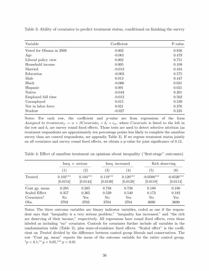
Table 3: Ability of covariates to predict treatment status, conditional on finishing the survey
Variable Coefficient P-value
Voted for Obama in 2008 0.003 0.856Age -0.001 0.479Liberal policy view 0.002 0.751Household income 0.005 0.109Married -0.013 0.434Education -0.003 0.575Male 0.013 0.447Black -0.066 0.031Hispanic 0.091 0.021Native -0.043 0.201Employed full time -0.012 0.502Unemployed 0.015 0.539Not in labor force 0.021 0.376Student -0.027 0.235
Notes: For each row, the coefficient and p-value are from regressions of the formAssigned to treatmentir = α + βCovariatei + δr + εir, where Covariate is listed to the left inthe row and δr are survey round fixed effects. Those tests are used to detect selective attrition (astreatment respondents are approximately ten percentage points less likely to complete the omnibussurvey than are control respondents, see appendix Table 3). If we regress treatment status jointlyon all covariates and survey round fixed effects, we obtain a p-value for joint significance of 0.12.
Table 4: Effect of omnibus treatment on opinions about inequality (“first-stage” outcomes)
Ineq. v. serious Ineq. increased Rich deserving
(1) (2) (3) (4) (5) (6)
Treated 0.102∗∗∗ 0.104∗∗∗ 0.119∗∗∗ 0.120∗∗∗ -0.0500∗∗∗ -0.0526∗∗∗
[0.0154] [0.0144] [0.0130] [0.0128] [0.0119] [0.0114]
Cont gp. mean 0.285 0.285 0.738 0.738 0.180 0.180Scaled Effect 0.357 0.365 0.539 0.540 0.173 0.182Covariates? No Yes No Yes No YesObs. 3703 3703 3704 3704 3690 3690
Notes: The three outcome variables are binary indicator variables, coded as one if the respon-dent says that “inequality is a very serious problem,” “inequality has increased,” and “the richare deserving of their income,” respectively. All regressions have round fixed effects, even thoselabeled as including “no” covariates. Controls for covariates further include all variables in therandomization table (Table 3), plus state-of-residence fixed effects. “Scaled effect” is the coeffi-cient on Treated divided by the difference between control group liberals and conservatives. Therow “Cont pg. mean” reports the mean of the outcome variable for the entire control group.∗p < 0.1,∗∗ p < 0.05,∗∗∗ p < 0.01
36
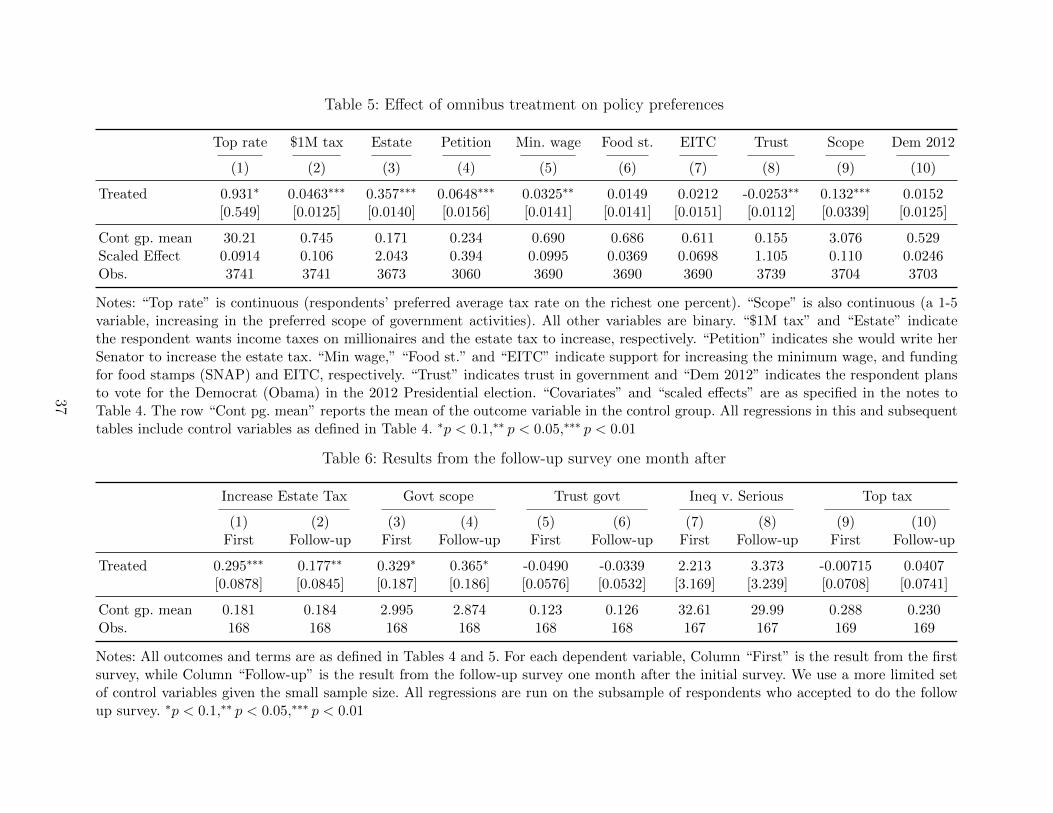
Table 5: Effect of omnibus treatment on policy preferences
Top rate $1M tax Estate Petition Min. wage Food st. EITC Trust Scope Dem 2012
(1) (2) (3) (4) (5) (6) (7) (8) (9) (10)
Treated 0.931∗ 0.0463∗∗∗ 0.357∗∗∗ 0.0648∗∗∗ 0.0325∗∗ 0.0149 0.0212 -0.0253∗∗ 0.132∗∗∗ 0.0152[0.549] [0.0125] [0.0140] [0.0156] [0.0141] [0.0141] [0.0151] [0.0112] [0.0339] [0.0125]
Cont gp. mean 30.21 0.745 0.171 0.234 0.690 0.686 0.611 0.155 3.076 0.529Scaled Effect 0.0914 0.106 2.043 0.394 0.0995 0.0369 0.0698 1.105 0.110 0.0246Obs. 3741 3741 3673 3060 3690 3690 3690 3739 3704 3703
Notes: “Top rate” is continuous (respondents’ preferred average tax rate on the richest one percent). “Scope” is also continuous (a 1-5variable, increasing in the preferred scope of government activities). All other variables are binary. “$1M tax” and “Estate” indicatethe respondent wants income taxes on millionaires and the estate tax to increase, respectively. “Petition” indicates she would write herSenator to increase the estate tax. “Min wage,” “Food st.” and “EITC” indicate support for increasing the minimum wage, and fundingfor food stamps (SNAP) and EITC, respectively. “Trust” indicates trust in government and “Dem 2012” indicates the respondent plansto vote for the Democrat (Obama) in the 2012 Presidential election. “Covariates” and “scaled effects” are as specified in the notes toTable 4. The row “Cont pg. mean” reports the mean of the outcome variable in the control group. All regressions in this and subsequenttables include control variables as defined in Table 4. ∗p < 0.1,∗∗ p < 0.05,∗∗∗ p < 0.01
Table 6: Results from the follow-up survey one month after
Increase Estate Tax Govt scope Trust govt Ineq v. Serious Top tax
(1) (2) (3) (4) (5) (6) (7) (8) (9) (10)First Follow-up First Follow-up First Follow-up First Follow-up First Follow-up
Treated 0.295∗∗∗ 0.177∗∗ 0.329∗ 0.365∗ -0.0490 -0.0339 2.213 3.373 -0.00715 0.0407[0.0878] [0.0845] [0.187] [0.186] [0.0576] [0.0532] [3.169] [3.239] [0.0708] [0.0741]
Cont gp. mean 0.181 0.184 2.995 2.874 0.123 0.126 32.61 29.99 0.288 0.230Obs. 168 168 168 168 168 168 167 167 169 169
Notes: All outcomes and terms are as defined in Tables 4 and 5. For each dependent variable, Column “First” is the result from the firstsurvey, while Column “Follow-up” is the result from the follow-up survey one month after the initial survey. We use a more limited setof control variables given the small sample size. All regressions are run on the subsample of respondents who accepted to do the followup survey. ∗p < 0.1,∗∗ p < 0.05,∗∗∗ p < 0.01
37
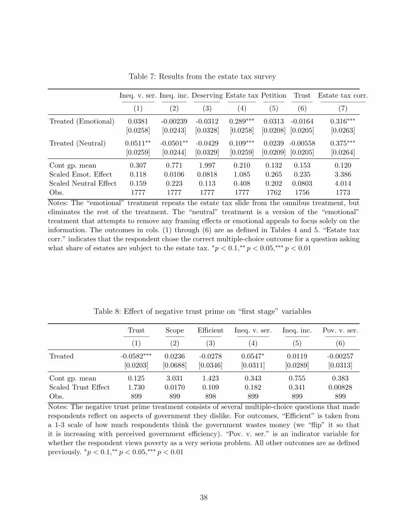
Table 7: Results from the estate tax survey
Ineq. v. ser. Ineq. inc. Deserving Estate tax Petition Trust Estate tax corr.
(1) (2) (3) (4) (5) (6) (7)
Treated (Emotional) 0.0381 -0.00239 -0.0312 0.289∗∗∗ 0.0313 -0.0164 0.316∗∗∗
[0.0258] [0.0243] [0.0328] [0.0258] [0.0208] [0.0205] [0.0263]
Treated (Neutral) 0.0511∗∗ -0.0501∗∗ -0.0429 0.109∗∗∗ 0.0239 -0.00558 0.375∗∗∗
[0.0259] [0.0244] [0.0329] [0.0259] [0.0209] [0.0205] [0.0264]
Cont gp. mean 0.307 0.771 1.997 0.210 0.132 0.153 0.120Scaled Emot. Effect 0.118 0.0106 0.0818 1.085 0.265 0.235 3.386Scaled Neutral Effect 0.159 0.223 0.113 0.408 0.202 0.0803 4.014Obs. 1777 1777 1777 1777 1762 1756 1773
Notes: The “emotional” treatment repeats the estate tax slide from the omnibus treatment, buteliminates the rest of the treatment. The “neutral” treatment is a version of the “emotional”treatment that attempts to remove any framing effects or emotional appeals to focus solely on theinformation. The outcomes in cols. (1) through (6) are as defined in Tables 4 and 5. “Estate taxcorr.” indicates that the respondent chose the correct multiple-choice outcome for a question askingwhat share of estates are subject to the estate tax. ∗p < 0.1,∗∗ p < 0.05,∗∗∗ p < 0.01
Table 8: Effect of negative trust prime on “first stage” variables
Trust Scope Efficient Ineq. v. ser. Ineq. inc. Pov. v. ser.
(1) (2) (3) (4) (5) (6)
Treated -0.0582∗∗∗ 0.0236 -0.0278 0.0547∗ 0.0119 -0.00257[0.0203] [0.0688] [0.0346] [0.0311] [0.0289] [0.0313]
Cont gp. mean 0.125 3.031 1.423 0.343 0.755 0.383Scaled Trust Effect 1.730 0.0170 0.109 0.182 0.341 0.00828Obs. 899 899 898 899 899 899
Notes: The negative trust prime treatment consists of several multiple-choice questions that maderespondents reflect on aspects of government they dislike. For outcomes, “Efficient” is taken froma 1-3 scale of how much respondents think the government wastes money (we “flip” it so thatit is increasing with perceived government efficiency). “Pov. v. ser.” is an indicator variable forwhether the respondent views poverty as a very serious problem. All other outcomes are as definedpreviously. ∗p < 0.1,∗∗ p < 0.05,∗∗∗ p < 0.01
38

Table 9: Effect of negative trust prime on outcome variables
$1M tax Est. tax Petition Min. wage Aid poor Food st. Housing Priv. char. Educ.
(1) (2) (3) (4) (5) (6) (7) (8) (9)
Treated -0.0421 -0.00168 -0.0602∗∗ -0.00428 -0.139∗∗ -0.153∗∗ -0.163∗∗∗ 0.187∗∗ 0.0615[0.0275] [0.0266] [0.0236] [0.0902] [0.0616] [0.0673] [0.0614] [0.0791] [0.0885]
Cont gp. mean 0.722 0.204 0.174 2.673 2.675 2.454 2.581 1.800 3.732Scaled Trust Effect 0.0949 0.00728 0.580 0.00531 0.128 0.119 0.133 0.169 0.265Obs. 899 895 899 899 899 899 899 850 874
Notes: The negative trust prime treatment consists of several multiple-choice questions that made respondents reflect on aspects ofgovernment they dislike. Outcome variables are defined as follows.“Aid poor” is a 1-4 categorical variable increasing in support forprograms that aid poor households. “Housing” is a 1-4 categorical variable increase in support for funding public housing programs.“Priv. char.” is an indicator of where (among a list of five policy approaches) the respondent puts “private charity” as a preferred methodfor addressing inequality (the variable increases in relative support for private charity with respect to the other outcomes). “Educ.” isdefined in a parallel manner for education spending. All other outcomes are as defined previously. ∗p < 0.1,∗∗ p < 0.05,∗∗∗ p < 0.01
Table 10: Effect of “emotional” treatment on outcome variables
Ineq. v. ser. Ineq. inc. Pov. v. ser. Min. wage Aid poor Food st. Housing Trust gov.
(1) (2) (3) (4) (5) (6) (7) (8)
Treated 0.0778∗∗∗ 0.0374 0.0971∗∗∗ 0.0280 0.147 0.189∗ 0.0473 -0.0132[0.0278] [0.0256] [0.0315] [0.0993] [0.0936] [0.101] [0.0944] [0.0215]
Cont gp. mean 0.307 0.771 0.316 2.529 2.127 1.811 2.064 0.144Scaled Poverty Effect 0.211 0.179 0.293 0.0283 0.0689 0.0973 0.0249 0.264Obs. 1825 1824 1204 899 899 899 899 1825
Notes: The “emotional” treatment aimed at creating empathy between the respondent and families living in poverty. Respondents weretold about poverty rates and had to fill out a minimum budget for a family like theirs living in the same city. Respondents were thenshown how their minimum budget compared to the poverty line. All outcomes are as defined previously. ∗p < 0.1,∗∗ p < 0.05,∗∗∗ p < 0.01
39

Table 11: Effect of policy treatment on outcome variables
Ineq. v. ser. Ineq. inc. Pov. v. ser. Min. wage Aid poor Food st. Housing Priv. char. Educ. Trust gov.
(1) (2) (3) (4) (5) (6) (7) (8) (9) (10)
Treated 0.0408 0.0289 -0.00872 0.304∗∗∗ 0.149 0.299∗∗∗ 0.244∗∗∗ -0.130∗ -0.117 -0.0349∗
[0.0268] [0.0255] [0.0269] [0.0960] [0.0909] [0.0977] [0.0906] [0.0704] [0.0782] [0.0206]
Cont gp. mean 0.307 0.771 0.316 2.529 2.127 1.811 2.064 2.026 3.728 0.144Scaled Policy Effect 0.111 0.138 0.0263 0.308 0.0698 0.154 0.128 0.0731 0.155 0.698Obs. 1835 1834 1315 906 906 906 906 1266 1285 1835
Notes: The policy treatment aimed at creating empathy between the respondent and families living on a minimum wage. Respondentshad to fill out a minimum budget for a family like theirs living in the same city. Respondents were then shown how their minimumbudget compared to the minimum wage and how food stamps adds $150 per person/month to the budget of such a family. All outcomesare as defined previously. ∗p < 0.1,∗∗ p < 0.05,∗∗∗ p < 0.01
40

Online Appendix (Not for Publication)
A Detailed Description of the Experiment
A.1 Omnibus Treatment Description
This Section describes in detail the omnibus experiment. The omnibus treatment experimentwas carried out in 4 separate rounds from January 2011 to August 2012. The structure ofthe experiment was as follows:(1) Background socio-economic questions including age, gender, race, marital status, chil-dren, state of residence, education, household income, work status, whether the respondentconsiders himself conservative or liberal on economic policy, voting choice in 2008 presiden-tial election.(2) Randomized treatment showing information on inequality, the estate tax, and tax policyshown solely to the treatment group. Those treatments are illustrated through screenshotsin appendix Figures 1, 2, 3, and 4.(3) Set of questions on inequality, taxes and transfers, policy views and 2012 voting plans.Those questions are listed in detail after the screenshots.
Surveys were openly posted on mTurk and their description stated that they would pay$1.50 for approximately 15 minutes of survey time, i.e., a $6 hourly wage. People were freeto drop out any time or take up to one hour to answer all questions.
Round 3 was conducted with CT Marketing Group instead of mTurk at a cost of $5 perrespondent. The survey software remained exactly the same.
The link to this survey is: https://hbs.qualtrics.com/SE/?SID=SV_77fSvTy12ZSBihn
List of all Outcome Questions
Note: Sentences in italic were not seen by the respondents. Bold fonts are just labels for eachsection. Sentences in normal font are exactly as they appeared in the survey.
Tax rate questions:
1. Choose the tax rate on the top 1%, next 9%, next 40% and bottom 50% (see screenshot).2. Do you think top income tax rates were higher in the 1950s and 1960s than they are
today?3. As you may know, there have been proposals recently to decrease the federal deficit
by raising income taxes on millionaires. Do you think income taxes on millionaires shouldbe increased, stay the same or decreased?
4. The Federal Estate tax (also known as the Death Tax) is a tax imposed on the transferof wealth from a deceased person to his or her heirs. Do you think the Federal Estate taxshould be decreased, left as is or increased?
First stage questions on knowledge and perceptions of inequality:5. Do you think annual economic growth was faster in the period 1980-2010 than in the
period 1933-1980?6. Do you think inequality is a serious problem in America?7. Do you think income inequality in the US has increased or decreased in recent decades?8. Are you satisfied with your current income?9. Do you think that the very high earners in our society deserve their high incomes?10. Which statement do you agree with most? (A: ”One’s income and position in society
is mostly the result of one’s individual effort”/ B:”One’s income and position in society is toa large extent the outcome of elements outside of one’s control (for example, including butnot limited to family background, luck, health issues, etc..)?
41
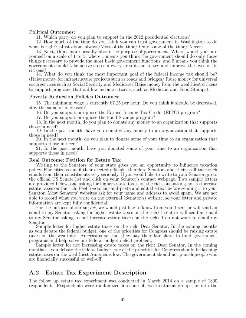
Political Outcomes:11. Which party do you plan to support in the 2012 presidential elections?12. How much of the time do you think you can trust government in Washington to do
what is right? (Just about always/Most of the time/ Only some of the time/ Never)13. Next, think more broadly about the purpose of government. Where would you rate
yourself on a scale of 1 to 5, where 1 means you think the government should do only thosethings necessary to provide the most basic government functions, and 5 means you think thegovernment should take active steps in every area it can to try and improve the lives of itscitizens?
14. What do you think the most important goal of the federal income tax should be?(Raise money for infrastructure projects such as roads and bridges/ Raise money for universalsocia services such as Social Security and Medicare/ Raise money from the wealthiest citizensto support programs that aid low-income citizens, such as Medicaid and Food Stamps).
Poverty Reduction Policies Outcomes:
15. The minimum wage is currently $7.25 per hour. Do you think it should be decreased,stay the same or increased?
16. Do you support or oppose the Earned Income Tax Credit (EITC) program?17. Do you support or oppose the Food Stamps program?18. In the next month, do you plan to donate any money to an organization that supports
those in need?19. In the past month, have you donated any money to an organization that supports
those in need?20. In the next month, do you plan to donate some of your time to an organization that
supports those in need?21. In the past month, have you donated some of your time to an organization that
supports those in need?
Real Outcome: Petition for Estate TaxWriting to the Senators of your state gives you an opportunity to influence taxation
policy. Few citizens email their elected officials, therefore Senators and their staff take suchemails from their constituents very seriously. If you would like to write to your Senator, go tothe official US Senate list and click on your Senator’s contact webpage. Two sample lettersare provided below, one asking for higher estate taxes on the rich, one asking not to increaseestate taxes on the rich. Feel free to cut-and-paste and edit the text before sending it to yourSenator. Most Senators’ websites ask for your name and address to avoid spam. We are notable to record what you write on the external (Senator’s) website, so your letter and privateinformation are kept fully confidential.
For the purpose of our survey, we would just like to know from you: I sent or will send anemail to my Senator asking for higher estate taxes on the rich/ I sent or will send an emailto my Senator asking to not increase estate taxes on the rich/ I do not want to email mySenator
Sample letter for higher estate taxes on the rich: Dear Senator, In the coming monthsas you debate the federal budget, one of the priorities for Congress should be raising estatetaxes on the wealthiest Americans so that they pay their fair share to fund governmentprograms and help solve our federal budget deficit problem.
Sample letter for not increasing estate taxes on the rich: Dear Senator, In the comingmonths as you debate the federal budget, one of the priorities for Congress should be keepingestate taxes on the wealthiest Americans low. The government should not punish people whoare financially successful or well-off.
A.2 Estate Tax Experiment Description
The follow up estate tax experiment was conducted in March 2014 on a sample of 1800respondents. Respondents were randomized into one of two treatment groups, or into the
42

control group. The first treatment group saw the same screen as in the omnibus treatment(only the part regarding the estate tax), as in appendix Figure 4. The second group saw aplain explanation for the estate tax, as in appendix Figure 6.
The link to this experiment is: https://hbs.qualtrics.com/SE/?SID=SV_0vOecp2MDPBpInb
List of all Outcome Questions
Note: Sentences in italic were not seen by the respondents. Bold fonts are just labels for eachsection. Sentences in normal font are exactly as they appeared in the survey.
1. Choose the tax rate on the top 1%, next 9%, next 40% and bottom 50% (see screenshot).2. Do you think income inequality in the United States has increased or decreased since
1980?3. Do you think inequality is a serious problem in America?4. The Federal Estate Tax is a tax imposed on the transfer of wealth from a deceased
person to his or her heirs. What percentage of people who die have to pay the Federal Estatetax? If you don’t know, just give your best guess.
5. Do you think poverty is a serious problem in America?6. Do you think that the very high earners in our society deserve their high incomes?7. Do you think the federal estate tax should be decreased, left as is or increased? (Recall
that the federal estate tax is a tax imposed on the transfer of wealth from a deceased personto his or her heirs.)
8. As you may know, there have been proposals recently to decrease the federal deficitby raising income taxes on millionaires. Do you think income taxes on millionaires shouldbe increased, stay the same or decreased?
9. Which of the tools below do you consider the best to address inequality in the UnitedStates? Please drag and drop the items to the box on the right and rank them in yourpreferred order. Your preferred method for addressing inequality should be at the top, yourleast preferred one at the bottom. [Education Policies, Private Charity, Progressive Taxes,Government Transfers (e.g., food stamps, Medicaid,..), Government regulation (e.g., minwage, caps on top compensation,...)]
10. Should the federal government increase or decrease spending on aid to the poor?11. The federal minimum wage is currently $7.25 per hour. Do you think it should be
decreased, stay the same or increased?12. Should the federal government increase or decrease its spending on public housing for
low income families?13. Should the federal government increase or decrease its spending on food stamps?
(Food stamps provide financial assistance for food purchasing to families and individualswith low or no income.)
14. Petition for Estate Tax : same as in A.115. Which party do you plan to support in the 2014 congressional elections?16. How much of the time do you think you can trust government in Washington to do
what is right?17. Next, think more broadly about the purpose of government. Where would you rate
yourself on a scale of 1 to 5, where 1 means you think the government should do only thosethings necessary to provide the most basic government functions, and 5 means you think thegovernment should take active steps in every area it can to try and improve the lives of itscitizens?
18. Do you think that people in the government waste a lot of money we pay in taxes,waste some of it, or don’t waste very much of it?”
19. How do you feel about the following statement: ”Currently, the federal governmentis very effective in limiting fraud, waste and abuse in the programs it administers”?
20. How do you feel about the following statement: ”Politicians in Washington work toenrich themselves and their largest campaign contributors, instead of working for the benefitof the majority of citizens”?
43
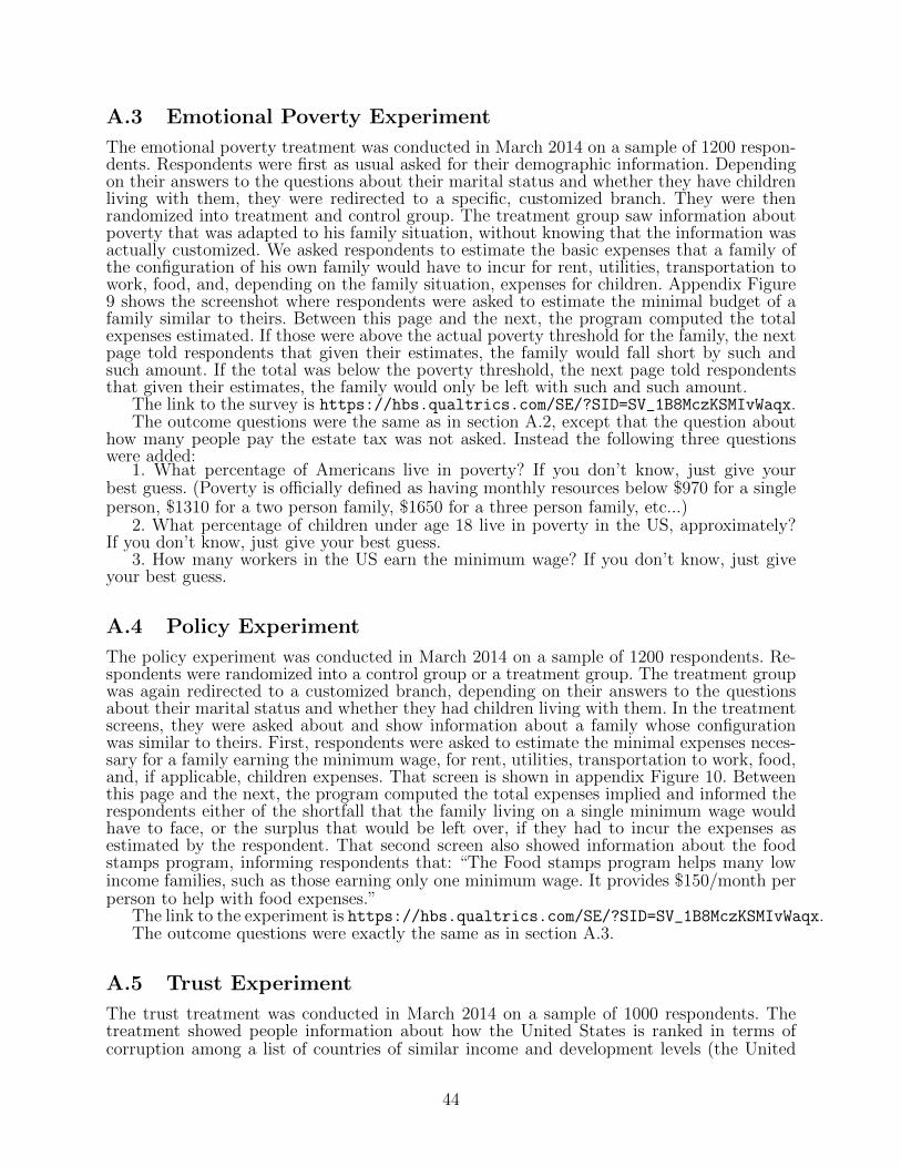
A.3 Emotional Poverty Experiment
The emotional poverty treatment was conducted in March 2014 on a sample of 1200 respon-dents. Respondents were first as usual asked for their demographic information. Dependingon their answers to the questions about their marital status and whether they have childrenliving with them, they were redirected to a specific, customized branch. They were thenrandomized into treatment and control group. The treatment group saw information aboutpoverty that was adapted to his family situation, without knowing that the information wasactually customized. We asked respondents to estimate the basic expenses that a family ofthe configuration of his own family would have to incur for rent, utilities, transportation towork, food, and, depending on the family situation, expenses for children. Appendix Figure9 shows the screenshot where respondents were asked to estimate the minimal budget of afamily similar to theirs. Between this page and the next, the program computed the totalexpenses estimated. If those were above the actual poverty threshold for the family, the nextpage told respondents that given their estimates, the family would fall short by such andsuch amount. If the total was below the poverty threshold, the next page told respondentsthat given their estimates, the family would only be left with such and such amount.
The link to the survey is https://hbs.qualtrics.com/SE/?SID=SV_1B8MczKSMIvWaqx.The outcome questions were the same as in section A.2, except that the question about
how many people pay the estate tax was not asked. Instead the following three questionswere added:
1. What percentage of Americans live in poverty? If you don’t know, just give yourbest guess. (Poverty is officially defined as having monthly resources below $970 for a singleperson, $1310 for a two person family, $1650 for a three person family, etc...)
2. What percentage of children under age 18 live in poverty in the US, approximately?If you don’t know, just give your best guess.
3. How many workers in the US earn the minimum wage? If you don’t know, just giveyour best guess.
A.4 Policy Experiment
The policy experiment was conducted in March 2014 on a sample of 1200 respondents. Re-spondents were randomized into a control group or a treatment group. The treatment groupwas again redirected to a customized branch, depending on their answers to the questionsabout their marital status and whether they had children living with them. In the treatmentscreens, they were asked about and show information about a family whose configurationwas similar to theirs. First, respondents were asked to estimate the minimal expenses neces-sary for a family earning the minimum wage, for rent, utilities, transportation to work, food,and, if applicable, children expenses. That screen is shown in appendix Figure 10. Betweenthis page and the next, the program computed the total expenses implied and informed therespondents either of the shortfall that the family living on a single minimum wage wouldhave to face, or the surplus that would be left over, if they had to incur the expenses asestimated by the respondent. That second screen also showed information about the foodstamps program, informing respondents that: “The Food stamps program helps many lowincome families, such as those earning only one minimum wage. It provides $150/month perperson to help with food expenses.”
The link to the experiment is https://hbs.qualtrics.com/SE/?SID=SV_1B8MczKSMIvWaqx.The outcome questions were exactly the same as in section A.3.
A.5 Trust Experiment
The trust treatment was conducted in March 2014 on a sample of 1000 respondents. Thetreatment showed people information about how the United States is ranked in terms ofcorruption among a list of countries of similar income and development levels (the United
44
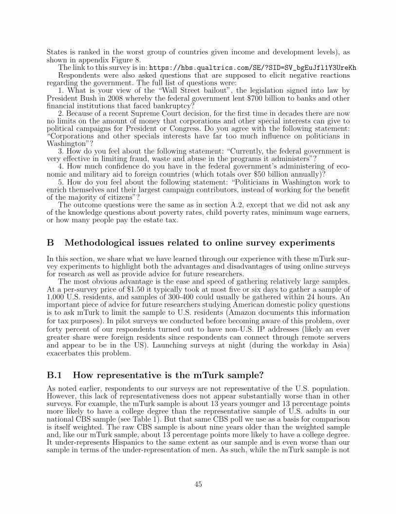
States is ranked in the worst group of countries given income and development levels), asshown in appendix Figure 8.
The link to this survey is in: https://hbs.qualtrics.com/SE/?SID=SV_bgEuJfl1Y3UreKhRespondents were also asked questions that are supposed to elicit negative reactions
regarding the government. The full list of questions were:1. What is your view of the “Wall Street bailout”, the legislation signed into law by
President Bush in 2008 whereby the federal government lent $700 billion to banks and otherfinancial institutions that faced bankruptcy?
2. Because of a recent Supreme Court decision, for the first time in decades there are nowno limits on the amount of money that corporations and other special interests can give topolitical campaigns for President or Congress. Do you agree with the following statement:“Corporations and other specials interests have far too much influence on politicians inWashington”?
3. How do you feel about the following statement: “Currently, the federal government isvery effective in limiting fraud, waste and abuse in the programs it administers”?
4. How much confidence do you have in the federal government’s administering of eco-nomic and military aid to foreign countries (which totals over $50 billion annually)?
5. How do you feel about the following statement: “Politicians in Washington work toenrich themselves and their largest campaign contributors, instead of working for the benefitof the majority of citizens”?
The outcome questions were the same as in section A.2, except that we did not ask anyof the knowledge questions about poverty rates, child poverty rates, minimum wage earners,or how many people pay the estate tax.
B Methodological issues related to online survey experiments
In this section, we share what we have learned through our experience with these mTurk sur-vey experiments to highlight both the advantages and disadvantages of using online surveysfor research as well as provide advice for future researchers.
The most obvious advantage is the ease and speed of gathering relatively large samples.At a per-survey price of $1.50 it typically took at most five or six days to gather a sample of1,000 U.S. residents, and samples of 300-400 could usually be gathered within 24 hours. Animportant piece of advice for future researchers studying American domestic policy questionsis to ask mTurk to limit the sample to U.S. residents (Amazon documents this informationfor tax purposes). In pilot surveys we conducted before becoming aware of this problem, overforty percent of our respondents turned out to have non-U.S. IP addresses (likely an evergreater share were foreign residents since respondents can connect through remote serversand appear to be in the US). Launching surveys at night (during the workday in Asia)exacerbates this problem.
B.1 How representative is the mTurk sample?
As noted earlier, respondents to our surveys are not representative of the U.S. population.However, this lack of representativeness does not appear substantially worse than in othersurveys. For example, the mTurk sample is about 13 years younger and 13 percentage pointsmore likely to have a college degree than the representative sample of U.S. adults in ournational CBS sample (see Table 1). But that same CBS poll we use as a basis for comparisonis itself weighted. The raw CBS sample is about nine years older than the weighted sampleand, like our mTurk sample, about 13 percentage points more likely to have a college degree.It under-represents Hispanics to the same extent as our sample and is even worse than oursample in terms of the under-representation of men. As such, while the mTurk sample is not
45

representative, neither are other standard polls (though some of the biases, such as age, arein opposite directions from standard polls).
As noted in the text, the American Life Panel is more representative than the mTurksample. However, this sample is much smaller and roughly 30 times more expensive thanmTurk.
B.2 How serious is attrition in the mTurk sample?
As noted earlier, for the omnibus treatment, we have an overall attrition rate (the share ofrespondents who start but do not finish the survey) of 22 percent: a 21 percent rate for theCT Marketing Group survey and a 22 percent rate for the mTurk surveys. In fact, whenwe compare surveys 4 and 5—which were in the field at the same time, with the former onmTurk and the latter on CT Marketing Group—attrition is actually lower on mTurk. EvenGallup has an attrition rate of nine percent on its 15-minute Daily Poll.43 Given that oursurvey requires people to read through informational treatments, we suspect that a pureopinion survey conducted on mTurk would have a lower attrition rate.
The omnibus survey has differential attrition between treatment and control, probablybecause of the relatively long length of the treatment (respondents had to scroll through6 treatment pages in the omnibus survey). Importantly, the follow-up surveys do not havesuch a differential attrition because the treatment was much shorter (2 pages at most) sothat there was no noticeable length difference between the treatment and control group.
A related point is that researchers using this methodology should ask background ques-tions first. In settings with little to no attrition, background questions can ideally be askedat the very end to avoid priming, but given the importance of assessing non-random attri-tion, it may be preferable for online survey experiments to ask demographic and backgroundquestions at the outset.
B.3 How many unique observations can one collect on mTurk?
Although the exact number of workers registered on mTurk is not publicly reported, thepool is thought to be quite large, approximately 500,000.
However, the pool available for any given survey experiment is more limited. First, work-ers select into tasks voluntarily, choosing among types of tasks. As a result, the pool ofworkers interested in survey experiments is more limited. Indeed survey experiments aretypically longer than a standard task on mTurk and might require more attention. Second,we filter workers based on past ratings: this is to avoid careless workers who consistentlydo not complete tasks properly and have been rated badly by previous amazon mTurk re-questers (i.e., employers on mTurk). Third, the pool of registered workers is not online allthe time. Many workers could be working for a few weeks, then switch to another occupa-tion, and potentially come back later or only work during some times of the year, month,or week. Finally, there is competition between tasks. Many tasks are posted simultaneouslyon the platform and workers have to search for each individual task. Large sample surveyexperiments sometimes fall lower in the list and are less visible to workers (although, oneway to make it more visible and which we employ, is to stop and relaunch the survey severaltimes so that it moves back up to the top of the list of tasks).
We always exclude workers who have already taken one of our survey experiments in thepast to avoid any spillovers from previous treatments. Hence, we need a fresh sample everytime. Accordingly, we noticed that when we launch a survey experiment a couple of weeksafter a previous one, we easily get a large sample very quickly. However, when we repeatedlylaunch experiments one after the other, the rate at which we get workers slows down.
43Email correspondence when Jeffrey Jones at Gallup, January 16, 2013. The nine-percent figurerefers to all Daily Polls from 2012.
46

To mitigate the constraint of being unable to reach a sufficiently large sample of workers,researchers can do all of the following: a) leave sufficient times between survey dates, b)pay sufficiently high wages to make the tasks competitive relative to others, c) keep surveytime short, d) choose more generic titles for the task, such as “Opinion Survey” rather than“Academic Research Survey in Economics.” However, researchers should be warned thateven after taking these steps, survey samples are not unlimited in mTurk and if “fresh”respondents are needed for each survey date a large share of respondents clicking on the taskwill be screened out (or will need to be dropped ex-post based on repeated mTurk workerIDs).
47
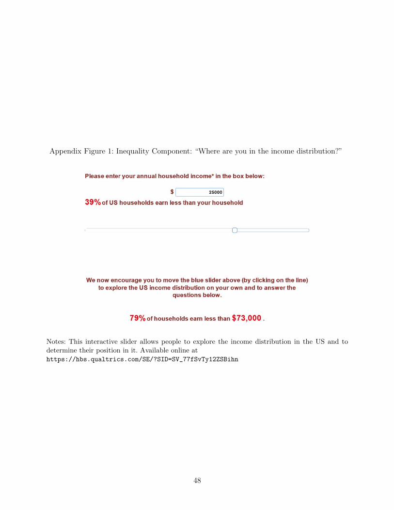
Appendix Figure 1: Inequality Component: “Where are you in the income distribution?”
Notes: This interactive slider allows people to explore the income distribution in the US and todetermine their position in it. Available online athttps://hbs.qualtrics.com/SE/?SID=SV_77fSvTy12ZSBihn
48
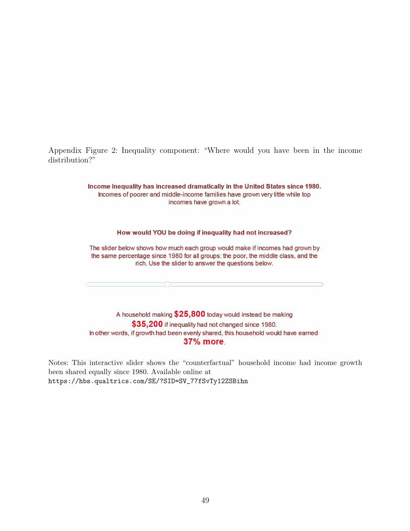
Appendix Figure 2: Inequality component: “Where would you have been in the incomedistribution?”
Notes: This interactive slider shows the “counterfactual” household income had income growthbeen shared equally since 1980. Available online athttps://hbs.qualtrics.com/SE/?SID=SV_77fSvTy12ZSBihn
49
Appendix Figure 3: Taxes component: Correlation between growth and top tax rates overtime
50

Appendix Figure 4: Showing information about the estate tax
Notes: Available online athttps://hbs.qualtrics.com/SE/?SID=SV_77fSvTy12ZSBihn
51

Appendix Figure 5: Preferred tax rates outcome
Notes: Available online athttps://hbs.qualtrics.com/SE/?SID=SV_77fSvTy12ZSBihn
52

Appendix Figure 6: Neutral information about the estate tax
Source: Calculations based on IRS Estate Tax Statistics
Neutral Treatment
These page timer metrics will not be displayed to the recipient.
First Click: 0 seconds.
Last Click: 0 seconds.
Page Submit: 0 seconds.
Click Count: 0 clicks.
The Federal Estate Tax applies when a deceased person leaves more than $5 million in wealth to his or her heirs.Wealth left to a spouse or charitable organizations is exempt from estate tax.
Only 1 person out of 1000 is wealthy enough to face the estate tax.
Average Americans have far less than $5 million in wealth when they die, so the estate tax does not affect them and theycan pass on their property to their children tax-free.
Source: Calculations based on IRS Estate Tax Statistics
Control Group
Qualtrics Survey Software https://s.qualtrics.com/ControlPanel/Ajax.php?action=GetSurve...
4 of 11 4/13/14 4:44 PM
Notes: Available online athttps://hbs.qualtrics.com/SE/?SID=SV_0vOecp2MDPBpInb
53

Appendix Figure 7: A word cloud based on open-ended responses to the question “How muchof the time can you trust the government in Washington to do what is right?”
Notes: Based on the pilot group survey on mTurk described in Section 5.2.
54

Appendix Figure 8: Negative information about corruption in the U.S.
Q75How do you feel about the following statement: "Politicians in Washington work to enrichthemselves and their largest campaign contributors, instead of working for the benefit of themajority of citizens"?
Strongly agree Agree Disagree Strongly disagree
Page Break
Q67Each year, the non-partisan organization Transparency International rates countries based on theamount of government corruption. When the US is compared to countries with similar levels ofincome and development how do you think it ranks?
The best 6 Better than average Worse than average The worst 6
Page Break
Q68These are the actual results from the report:
Qualtrics Survey Software https://s.qualtrics.com/ControlPanel/?ClientAction=EditSurve...
2 of 3 6/15/14 6:43 AM
Notes: Available online athttps://hbs.qualtrics.com/SE/?SID=SV_bgEuJfl1Y3UreKh
55
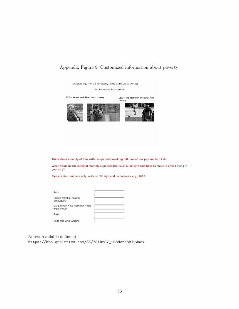
Appendix Figure 9: Customized information about poverty
Think about a family of four with two parents working full time at low pay and two kids. What would be the minimal monthly expenses that such a family would have to make to afford living inyour city? Please enter numbers only, with no "$" sign and no commas, e.g., 1000.
Rent
Utilities (electric, heating,cable/phone)
Car payment + car insurance + gasto go to work
Food
Child care while working
Married 2 kids Poverty Block 2
50 million of Americans, or 16% of the population, are living in poverty. For a family of four with two children, the povertythreshold is $1990/month.
Based on the numbers you gave, the family at the poverty threshold would be left with only ${InvalidExpression}-${q://QID535/ChoiceTextEntryValue/2}-${q://QID535/ChoiceTextEntryValue/3}-${q://QID535/ChoiceTextEntryValue/4}-${q://QID535/ChoiceTextEntryValue/5}}/month for all other expenses
Qualtrics Survey Software https://s.qualtrics.com/ControlPanel/Ajax.php?action=GetSurve...
18 of 37 4/2/14 11:04 AM
Notes: Available online athttps://hbs.qualtrics.com/SE/?SID=SV_1B8MczKSMIvWaqx
56

Appendix Figure 10: Customized information about policies
health care.
Single no kids control
Please click on "Next".
Married kids block 1
Think about a family of four with one parent working full time at the minimum wage and two kids. What would be the minimal monthly expenses that such a family would have to make to afford livingwhere you live? Please enter numbers only, with no "$" sign and no commas, e.g., 1000.
Rent
Utilities (electric, heating,cable/phone)
Transportation (public transit fareand/or car payments, insurance,gas…)
Food
Expenses related to children
Married kids block 2
The current federal minimum wage is $7.25/hour. That’s a net of $1,100/month when working 40 hours/week.
About 6 million US workers are paid the minimum wage. Based on the numbers you gave, the family of four with one minimum wage worker and 2 children would be left with only
${Invalid Expression}-${q://QID455/ChoiceTextEntryValue/2}-${q://QID455/ChoiceTextEntryValue
Qualtrics Survey Software https://s.qualtrics.com/ControlPanel/Ajax.php?action=GetSurve...
16 of 37 4/2/14 11:04 AM
Notes: Available online athttps://hbs.qualtrics.com/SE/?SID=SV_1B8MczKSMIvWaqx
57

Appendix Table 1: Share of treatment respondents correctly answering basic comprehensionquestions
(1)Percent that answered correctly
Pct of households earn less than 386,000 0.852Pct of households earn less than 108,000 0.843Pct of households earn less than 33,800 0.826Household now making 386,000 would be making... 0.464Household now making 108,000 would be making... 0.843Household now making 33,800 would be making... 0.800
Observations 1142
Notes: This table displays the percent of respondents who answered correctly to the comprehensionquestions during the treatment (see the treatment screenshots in the Appendix for the completewording and outlay of these questions.
Appendix Table 2: Ability of covariates to predict whether respondents’ finish the survey
Variable Coeff P-val
Voted for Obama in 2008 0.014 0.227Age -0.003 0.000Liberal policy view 0.002 0.676Household income 0.001 0.449Married 0.008 0.480Education -0.001 0.724Male 0.018 0.105Black -0.006 0.765Hispanic 0.072 0.007Native -0.011 0.624Employed full time -0.008 0.483Unemployed 0.024 0.145Not in labor force -0.029 0.055Student 0.023 0.137Treatment Group -0.113 0.000
Notes: For each row, the coefficient and p-value are from regressions of the form Finishedir =α+βCovariatei + δr + εir, where Covariate is listed to the left in the row and δr are survey roundfixed effects.
58

Appendix Table 3: Attrition by survey round
Survey Attrition Obs. (Completed)Control Treatment Differential
Omnibus 0.09 0.21 0.11 4045Estate Tax 0.06 0.03 -0.03 1760Trust 0.03 0.02 -0.01 901Poverty 0.06 0.02 -0.04 1825Policy 0.06 0.04 -0.02 1837
Notes: Note that the attrition numbers count those respondents who started and continued longenough to be at least assigned a treatment status. Respondents could drop out before being assignedto treatment for a variety of reasons, including that they were not U.S. citizens (albeit U.S. residents)or did not agree with the consent form.
59

Appendix Table 4: Effect of omnibus treatment on all outcomes, part 1
Ineq vs. Ineq. inc. Deserving Top tax Mill. tax Estate tax Petition Min. wage Food stamps EITC Trust Active.
(1) (2) (3) (4) (5) (6) (7) (8) (9) (10) (11) (12)
Treated 0.104∗∗∗ 0.120∗∗∗ -0.127∗∗∗ 0.931∗ 0.0463∗∗∗ 0.357∗∗∗ 0.0648∗∗∗ 0.0325∗∗ 0.0149 0.0212 -0.0253∗∗ 0.132∗∗∗
[0.0144] [0.0128] [0.0188] [0.549] [0.0125] [0.0140] [0.0156] [0.0141] [0.0141] [0.0151] [0.0112] [0.0339]
Cont gp. mean 0.285 0.738 2.002 30.21 0.745 0.171 0.234 0.690 0.686 0.611 0.155 3.076Scaled Effect 0.365 0.540 0.312 0.0914 0.106 2.043 0.394 0.0995 0.0369 0.0698 1.105 0.110Obs. 3703 3704 3690 3741 3741 3673 3060 3690 3690 3690 3739 3704
Notes: The first three outcome variables are binary indicator variables, coded as one if the respondent says that “inequality is a very seriousproblem,” “inequality has increased,” and “the rich are deserving of their income,” respectively. “Top rate” is continuous (respondents’preferred average tax rate on the richest one percent). “Mill. tax” and “Estate” indicate the respondent wants income taxes on millionairesand the estate tax to increase, respectively. “Petition” indicates she would write her Senator to increase the estate tax. “Min wage,” “Foodst.” and “EITC” indicate support for increasing the minimum wage, and funding for SNAP and EITC, respectively. “Trust” indicatestrust in government and “Active” indicates the respondent favors a broad range of interventions by the government. “Covariates” and“scaled effects” are as specified in the notes to Table 4. The row “Cont pg. mean” reports the mean of the outcome variable in the controlgroup. ∗p < 0.1,∗∗ p < 0.05,∗∗∗ p < 0.01
60

Appendix Table 5: Effect of omnibus treatment on all outcomes, part 2
Dem. 2012 Taxes redistr. Growth Tax 1950 Satisfied Money charity Money given Time charity Time given
(1) (2) (3) (4) (5) (6) (7) (8) (9)
Treated 0.0152 0.0396∗∗∗ 0.137∗∗∗ -0.0114∗ -0.0266 -0.00717 -0.00565 -0.00188 0.00655[0.0125] [0.0132] [0.0160] [0.00646] [0.0264] [0.0157] [0.0158] [0.0160] [0.0157]
Cont gp. mean 0.529 0.199 0.437 0.0616 2.881 1.441 1.477 1.520 1.622Scaled Effect 0.0246 0.314 0.946 0.487 0.102 0.167 0.0823 0.0219 0.255Obs. 3703 3700 3696 3698 3690 3681 3683 3684 3684
Notes: “Dem 2012” indicates the respondent plans to vote for the Democrat (Obama) in the 2012 Presidential election. “Taxes redistr.”indicates that the respondent thinks the role of income taxes is to redistribute income. “Growth” indicates that the respondent correctlyreplied to the question of whether growth was higher in 1933-1980 than in 1980-2000. “Tax 1950” indicates that the respondent correctlyreplied to the question whether top income taxes were higher in the 1950s than today. “Satisfied” indicates whether the respondent issatisfied with his current income. “Money charity” (respectively, “Time charity”) is a dummy variable for whether the respondent plansto give money (respectively, time) to charity in the next month and “Money given” (respectively, “Time given”) indicates whether hehas already given money (respectively, time) in the past month. “Covariates” and “scaled effects” are as specified in the notes to Table4. The row “Cont pg. mean” reports the mean of the outcome variable in the control group. ∗p < 0.1,∗∗ p < 0.05,∗∗∗ p < 0.01
61
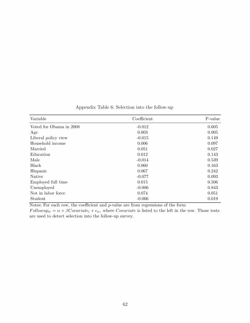
Appendix Table 6: Selection into the follow-up
Variable Coefficient P-value
Voted for Obama in 2008 -0.012 0.605Age 0.003 0.005Liberal policy view -0.015 0.149Household income 0.006 0.097Married 0.051 0.027Education 0.012 0.143Male -0.014 0.539Black 0.060 0.163Hispanic 0.067 0.242Native -0.077 0.093Employed full time 0.015 0.506Unemployed -0.006 0.843Not in labor force 0.074 0.051Student -0.066 0.019
Notes: For each row, the coefficient and p-value are from regressions of the formFollowupir = α+ βCovariatei + εir, where Covariate is listed to the left in the row. Those testsare used to detect selection into the follow-up survey.
62
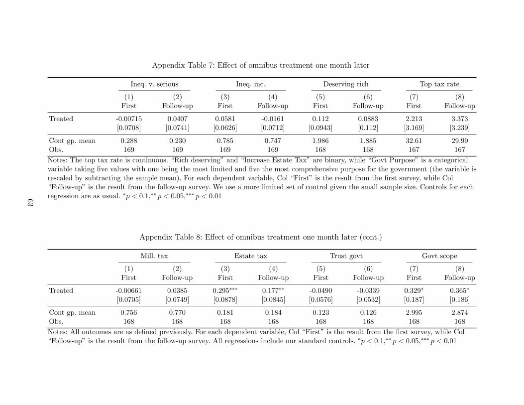
Appendix Table 7: Effect of omnibus treatment one month later
Ineq. v. serious Ineq. inc. Deserving rich Top tax rate
(1) (2) (3) (4) (5) (6) (7) (8)First Follow-up First Follow-up First Follow-up First Follow-up
Treated -0.00715 0.0407 0.0581 -0.0161 0.112 0.0883 2.213 3.373[0.0708] [0.0741] [0.0626] [0.0712] [0.0943] [0.112] [3.169] [3.239]
Cont gp. mean 0.288 0.230 0.785 0.747 1.986 1.885 32.61 29.99Obs. 169 169 169 169 168 168 167 167
Notes: The top tax rate is continuous. “Rich deserving” and “Increase Estate Tax” are binary, while “Govt Purpose” is a categoricalvariable taking five values with one being the most limited and five the most comprehensive purpose for the government (the variable isrescaled by subtracting the sample mean). For each dependent variable, Col “First” is the result from the first survey, while Col“Follow-up” is the result from the follow-up survey. We use a more limited set of control given the small sample size. Controls for eachregression are as usual. ∗p < 0.1,∗∗ p < 0.05,∗∗∗ p < 0.01
Appendix Table 8: Effect of omnibus treatment one month later (cont.)
Mill. tax Estate tax Trust govt Govt scope
(1) (2) (3) (4) (5) (6) (7) (8)First Follow-up First Follow-up First Follow-up First Follow-up
Treated -0.00661 0.0385 0.295∗∗∗ 0.177∗∗ -0.0490 -0.0339 0.329∗ 0.365∗
[0.0705] [0.0749] [0.0878] [0.0845] [0.0576] [0.0532] [0.187] [0.186]
Cont gp. mean 0.756 0.770 0.181 0.184 0.123 0.126 2.995 2.874Obs. 168 168 168 168 168 168 168 168
Notes: All outcomes are as defined previously. For each dependent variable, Col “First” is the result from the first survey, while Col“Follow-up” is the result from the follow-up survey. All regressions include our standard controls. ∗p < 0.1,∗∗ p < 0.05,∗∗∗ p < 0.01
63
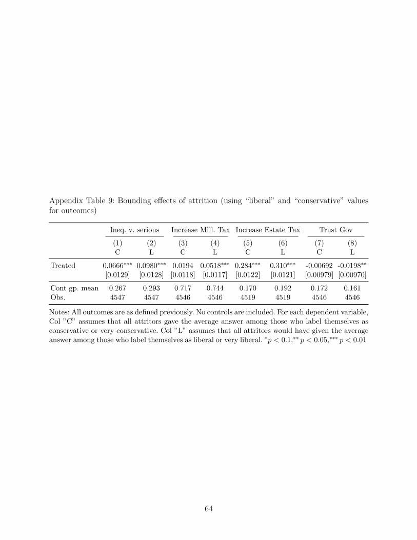
Appendix Table 9: Bounding effects of attrition (using “liberal” and “conservative” valuesfor outcomes)
Ineq. v. serious Increase Mill. Tax Increase Estate Tax Trust Gov
(1) (2) (3) (4) (5) (6) (7) (8)C L C L C L C L
Treated 0.0666∗∗∗ 0.0980∗∗∗ 0.0194 0.0518∗∗∗ 0.284∗∗∗ 0.310∗∗∗ -0.00692 -0.0198∗∗
[0.0129] [0.0128] [0.0118] [0.0117] [0.0122] [0.0121] [0.00979] [0.00970]
Cont gp. mean 0.267 0.293 0.717 0.744 0.170 0.192 0.172 0.161Obs. 4547 4547 4546 4546 4519 4519 4546 4546
Notes: All outcomes are as defined previously. No controls are included. For each dependent variable,Col ”C” assumes that all attritors gave the average answer among those who label themselves asconservative or very conservative. Col ”L” assumes that all attritors would have given the averageanswer among those who label themselves as liberal or very liberal. ∗p < 0.1,∗∗ p < 0.05,∗∗∗ p < 0.01
64

Appendix Table 10: Views on inequality and taxes for high- and low-attrition rounds in the omnibus surveys
Ineq. v. serious Ineq. increased Rich deserving Top tax rate Millionaire tax Estate tax
(1) (2) (3) (4) (5) (6) (7) (8) (9) (10) (11) (12)
Treated 0.0794∗∗∗ 0.117∗∗∗ 0.0849∗∗∗ 0.138∗∗∗ -0.00327 -0.0672∗∗∗ 0.155 2.003∗∗∗ 0.0154 0.0504∗∗∗ 0.421∗∗∗ 0.365∗∗∗
[0.0248] [0.0219] [0.0222] [0.0176] [0.0199] [0.0169] [1.031] [0.716] [0.0207] [0.0185] [0.0247] [0.0212]
Cont gp. mean 0.276 0.289 0.767 0.780 0.160 0.180 34.40 28.88 0.800 0.758 0.179 0.178Scaled Effect 0.278 0.387 0.475 0.615 0.0118 0.209 0.0131 0.203 0.0446 0.100 1.761 2.396Differential attrition? Low High Low High Low High Low High Low High Low HighObs. 1260 1635 1260 1636 1254 1631 1271 1650 1271 1650 1250 1626
Notes: All outcomes are as defined previously. “Differential attrition?” separates observations according to whether they were in ”Low”differential attrition round (round 4) or in ”High” differential attrition rounds (rounds 1, 2 and 3). Otherwise, all terminology followsthat in previous tables. ∗p < 0.1,∗∗ p < 0.05,∗∗∗ p < 0.01
Appendix Table 11: Opinions on other policies and views of government for high- and low-attrition rounds in the omnibussurveys
Min. wage EITC Food stamps Trust gov. Active gov.
(1) (2) (3) (4) (5) (6) (7) (8) (9) (10)
Treated 0.00695 0.0408∗ -0.0199 0.0260 0.0203 0.0197 -0.0553∗∗∗ 0.00269 0.0576 0.248∗∗∗
[0.0244] [0.0210] [0.0257] [0.0230] [0.0240] [0.0210] [0.0199] [0.0166] [0.0579] [0.0494]
Cont gp. mean 0.708 0.706 0.683 0.589 0.710 0.702 0.174 0.132 3.140 2.997Scaled Effect 0.0227 0.129 0.0679 0.0808 0.0490 0.0451 2.329 0.102 0.0441 0.195Differential attrition? Low High Low High Low High Low High Low HighObs. 1254 1631 1254 1631 1254 1631 1270 1649 1260 1636
Notes: See previous table. ∗p < 0.1,∗∗ p < 0.05,∗∗∗ p < 0.01
65
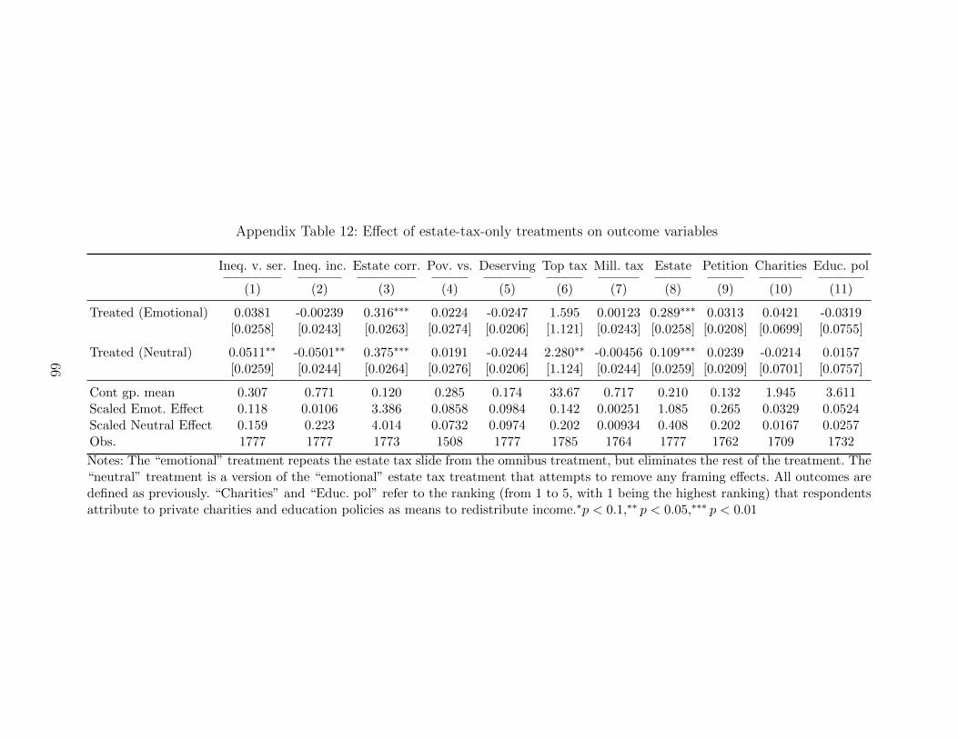
Appendix Table 12: Effect of estate-tax-only treatments on outcome variables
Ineq. v. ser. Ineq. inc. Estate corr. Pov. vs. Deserving Top tax Mill. tax Estate Petition Charities Educ. pol
(1) (2) (3) (4) (5) (6) (7) (8) (9) (10) (11)
Treated (Emotional) 0.0381 -0.00239 0.316∗∗∗ 0.0224 -0.0247 1.595 0.00123 0.289∗∗∗ 0.0313 0.0421 -0.0319[0.0258] [0.0243] [0.0263] [0.0274] [0.0206] [1.121] [0.0243] [0.0258] [0.0208] [0.0699] [0.0755]
Treated (Neutral) 0.0511∗∗ -0.0501∗∗ 0.375∗∗∗ 0.0191 -0.0244 2.280∗∗ -0.00456 0.109∗∗∗ 0.0239 -0.0214 0.0157[0.0259] [0.0244] [0.0264] [0.0276] [0.0206] [1.124] [0.0244] [0.0259] [0.0209] [0.0701] [0.0757]
Cont gp. mean 0.307 0.771 0.120 0.285 0.174 33.67 0.717 0.210 0.132 1.945 3.611Scaled Emot. Effect 0.118 0.0106 3.386 0.0858 0.0984 0.142 0.00251 1.085 0.265 0.0329 0.0524Scaled Neutral Effect 0.159 0.223 4.014 0.0732 0.0974 0.202 0.00934 0.408 0.202 0.0167 0.0257Obs. 1777 1777 1773 1508 1777 1785 1764 1777 1762 1709 1732
Notes: The “emotional” treatment repeats the estate tax slide from the omnibus treatment, but eliminates the rest of the treatment. The“neutral” treatment is a version of the “emotional” estate tax treatment that attempts to remove any framing effects. All outcomes aredefined as previously. “Charities” and “Educ. pol” refer to the ranking (from 1 to 5, with 1 being the highest ranking) that respondentsattribute to private charities and education policies as means to redistribute income.∗p < 0.1,∗∗ p < 0.05,∗∗∗ p < 0.01
66

Appendix Table 13: Effect of estate-tax-only treatment on outcome variables (cont.)
Min. wage Aid Food stamps Housing Trust Govt scope No waste Dem. 2014
(1) (2) (3) (4) (5) (6) (7) (8)
Treated (Emotional) 0.0529 0.109 0.0982 0.236∗∗∗ -0.0164 0.0172 -0.0281 0.0344[0.0865] [0.0837] [0.0861] [0.0824] [0.0205] [0.0585] [0.0303] [0.0213]
Treated (Neutral) -0.0838 0.0273 0.0628 0.127 -0.00558 0.0259 -0.0587∗ -0.00310[0.0870] [0.0842] [0.0866] [0.0829] [0.0205] [0.0587] [0.0303] [0.0213]
Cont gp. mean 2.608 2.130 1.797 1.927 0.153 3.074 1.456 0.470Scaled Emot. Effect 0.0913 0.0624 0.0534 0.140 0.235 0.0150 0.0896 0.0490Scaled Neutral Effect 0.145 0.0156 0.0341 0.0755 0.0803 0.0225 0.187 0.00441Obs. 1495 1495 1495 1495 1756 1756 1754 1756
Notes: See above. “No waste” takes values from 1 to 3, with 1 representing that the government is wasting a lot of tax revenue and 3that the government is not wasting much tax revenue at all. Note that the only statistically significant effect for a poverty-relatedoutcome is for increased public housing. We speculate that this effect is due to seeing the picture of the mansion in the “emotional”estate tax treatment (but not in the neutral treatment). ∗p < 0.1,∗∗ p < 0.05,∗∗∗ p < 0.01
67

Appendix Table 14: Effect of trust treatment on outcome variables
Ineq. v. ser. Ineq. inc. Pov. v. ser. Deserving Top tax Mill. tax Estate Petition
(1) (2) (3) (4) (5) (6) (7) (8)
Treated 0.0547∗ 0.0119 -0.00257 -0.0555∗∗ 0.490 -0.0421 -0.00168 -0.0602∗∗
[0.0311] [0.0289] [0.0313] [0.0239] [1.326] [0.0275] [0.0266] [0.0236]
Cont gp. mean 0.343 0.755 0.383 0.185 34.70 0.722 0.204 0.174Scaled Trust Effect 0.182 0.341 0.00828 0.204 0.0452 0.0949 0.00728 0.580Obs. 899 899 899 899 898 899 895 899
Notes: The negative trust prime treatment consists of several multiple-choice questions that made respondents reflect on aspects ofgovernment they dislike. All terms are defined as previously. ∗p < 0.1,∗∗ p < 0.05,∗∗∗ p < 0.01
Appendix Table 15: Effect of trust treatment on outcome variables (cont.)
Min wage Aid Food st. Housing Trust Active No waste Dem. 2014 Charity Educ. pol.
(1) (2) (3) (4) (5) (6) (7) (8) (9) (10)
Treated -0.00428 -0.139∗∗ -0.153∗∗ -0.163∗∗∗ -0.0582∗∗∗ 0.0236 -0.0278 -0.0462∗ 0.187∗∗ 0.0615[0.0902] [0.0616] [0.0673] [0.0614] [0.0203] [0.0688] [0.0346] [0.0258] [0.0791] [0.0885]
Cont gp. mean 2.673 2.675 2.454 2.581 0.125 3.031 1.423 0.479 1.800 3.732Scaled Trust Effect 0.00531 0.128 0.119 0.133 1.730 0.0170 0.109 0.0686 0.169 0.265Obs. 899 899 899 899 899 899 898 899 850 874
Notes: See above. ∗p < 0.1,∗∗ p < 0.05,∗∗∗ p < 0.01
68
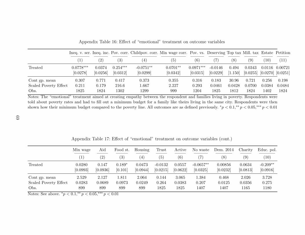
Appendix Table 16: Effect of “emotional” treatment on outcome variables
Ineq. v. ser. Ineq. inc. Pov. corr. Childpov. corr. Min wage corr. Pov. vs. Deserving Top tax Mill. tax Estate Petition
(1) (2) (3) (4) (5) (6) (7) (8) (9) (10) (11)
Treated 0.0778∗∗∗ 0.0374 0.254∗∗∗ -0.0751∗∗ 0.0701∗∗ 0.0971∗∗∗ -0.0146 0.494 0.0343 0.0116 0.00721[0.0278] [0.0256] [0.0312] [0.0299] [0.0342] [0.0315] [0.0229] [1.150] [0.0255] [0.0270] [0.0251]
Cont gp. mean 0.307 0.771 0.417 0.373 0.355 0.316 0.183 30.96 0.721 0.256 0.198Scaled Poverty Effect 0.211 0.179 216.6 1.667 2.227 0.293 0.0461 0.0428 0.0700 0.0384 0.0484Obs. 1825 1824 1302 1299 999 1204 1825 1812 1824 1402 1824
Notes: The “emotional” treatment aimed at creating empathy between the respondent and families living in poverty. Respondents weretold about poverty rates and had to fill out a minimum budget for a family like theirs living in the same city. Respondents were thenshown how their minimum budget compared to the poverty line. All outcomes are as defined previously. ∗p < 0.1,∗∗ p < 0.05,∗∗∗ p < 0.01
Appendix Table 17: Effect of “emotional” treatment on outcome variables (cont.)
Min wage Aid Food st. Housing Trust Active No waste Dem. 2014 Charity Educ. pol.
(1) (2) (3) (4) (5) (6) (7) (8) (9) (10)
Treated 0.0280 0.147 0.189∗ 0.0473 -0.0132 0.0557 -0.0657∗∗ 0.00856 0.0634 -0.209∗∗
[0.0993] [0.0936] [0.101] [0.0944] [0.0215] [0.0622] [0.0325] [0.0232] [0.0813] [0.0916]
Cont gp. mean 2.529 2.127 1.811 2.064 0.144 3.065 1.384 0.468 2.026 3.728Scaled Poverty Effect 0.0283 0.0689 0.0973 0.0249 0.264 0.0383 0.207 0.0125 0.0356 0.275Obs. 899 899 899 899 1825 1825 1407 1407 1165 1180
Notes: See above. ∗p < 0.1,∗∗ p < 0.05,∗∗∗ p < 0.01
69
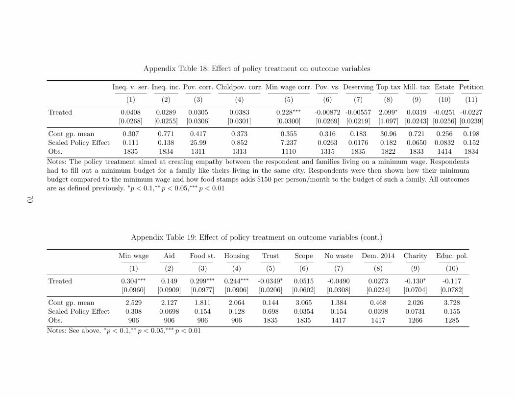
Appendix Table 18: Effect of policy treatment on outcome variables
Ineq. v. ser. Ineq. inc. Pov. corr. Childpov. corr. Min wage corr. Pov. vs. Deserving Top tax Mill. tax Estate Petition
(1) (2) (3) (4) (5) (6) (7) (8) (9) (10) (11)
Treated 0.0408 0.0289 0.0305 0.0383 0.228∗∗∗ -0.00872 -0.00557 2.099∗ 0.0319 -0.0251 -0.0227[0.0268] [0.0255] [0.0306] [0.0301] [0.0300] [0.0269] [0.0219] [1.097] [0.0243] [0.0256] [0.0239]
Cont gp. mean 0.307 0.771 0.417 0.373 0.355 0.316 0.183 30.96 0.721 0.256 0.198Scaled Policy Effect 0.111 0.138 25.99 0.852 7.237 0.0263 0.0176 0.182 0.0650 0.0832 0.152Obs. 1835 1834 1311 1313 1110 1315 1835 1822 1833 1414 1834
Notes: The policy treatment aimed at creating empathy between the respondent and families living on a minimum wage. Respondentshad to fill out a minimum budget for a family like theirs living in the same city. Respondents were then shown how their minimumbudget compared to the minimum wage and how food stamps adds $150 per person/month to the budget of such a family. All outcomesare as defined previously. ∗p < 0.1,∗∗ p < 0.05,∗∗∗ p < 0.01
Appendix Table 19: Effect of policy treatment on outcome variables (cont.)
Min wage Aid Food st. Housing Trust Scope No waste Dem. 2014 Charity Educ. pol.
(1) (2) (3) (4) (5) (6) (7) (8) (9) (10)
Treated 0.304∗∗∗ 0.149 0.299∗∗∗ 0.244∗∗∗ -0.0349∗ 0.0515 -0.0490 0.0273 -0.130∗ -0.117[0.0960] [0.0909] [0.0977] [0.0906] [0.0206] [0.0602] [0.0308] [0.0224] [0.0704] [0.0782]
Cont gp. mean 2.529 2.127 1.811 2.064 0.144 3.065 1.384 0.468 2.026 3.728Scaled Policy Effect 0.308 0.0698 0.154 0.128 0.698 0.0354 0.154 0.0398 0.0731 0.155Obs. 906 906 906 906 1835 1835 1417 1417 1266 1285
Notes: See above. ∗p < 0.1,∗∗ p < 0.05,∗∗∗ p < 0.01
70