How did bank holding companies prosper in the 1990s?directory.umm.ac.id/Data Elmu/jurnal/J-a/Journal Of Banking And Finance...How did bank holding companies prosper in the 1990s? Kevin

How did bank holding companies prosper in

the 1990s?

Kevin J. Stiroh *

Federal Reserve Bank of New York, 33 Liberty Street, NY 10045, USA

Received 14 July 1998; accepted 8 July 1999

Abstract

This paper examines the improved performance of US bank holding companies

(BHCs) from 1991 to 1997. Analysis of cost and pro®t functions using several alter-

native output speci®cations suggests that the gains were primarily due to productivity

growth and changes in scale economies. Various econometric methodologies yield

productivity growth of about 0.4% per year and the optimal size seems to have increased

in the 1990s era of deregulation, technological change, and ®nancial innovation. Esti-

mates of both productivity growth and economies of scale are robust across traditional

and non-traditional output speci®cations. Despite the overall success, however, sub-

stantial cost and pro®t ine�ciency existed for BHCs of all sizes in the 1990s. These

e�ciency estimates are particularly sensitive to the output speci®cation and failure to

account for non-traditional activities like o�-balance sheet (OBS) items leads pro®t

e�ciency, but not cost e�ciency, to be understated for the largest BHCs. Ó 2000

Elsevier Science B.V. All rights reserved.

JEL classi®cation: G21; D21

Keywords: Bank holding companies; Productivity; E�ciency

Journal of Banking & Finance 24 (2000) 1703±1745

www.elsevier.com/locate/econbase

* Tel.: +1-212-720-6633; fax: +1-212-720-8363.

E-mail address: [email protected] (K.J. Stiroh).

0378-4266/00/$ - see front matter Ó 2000 Elsevier Science B.V. All rights reserved.

PII: S 0 3 7 8 - 4 2 6 6 ( 9 9 ) 0 0 1 0 1 - 6

1. Introduction

Fundamental changes in regulation, macroeconomic shocks, and ®nancialinnovation have led to a major restructuring of the US commercial bankingindustry. Over the last decade, the number of FDIC-insured banking organi-zations declined by more than 35% even as total assets continued to grow andthe banking industry emerged from the crisis of the 1980s with strong per-formance and record pro®ts in the 1990s.

This paper examines the behavior of 661 bank holding companies (BHCs)from 1991 to 1997 to identify the sources of success in the 1990s. Cost and pro®tfunction analysis from alternative output speci®cations that include both tra-ditional lending activities and non-traditional activities like fee income or o�-balance sheet (OBS) items suggest that the improved performance re¯ects acombination of productivity growth and scale economies. Persistent ®rm-leveline�ciency, however, prevented even larger gains. The large literature on thee�ciency of ®nancial institutions has primarily focused on individual com-mercial banks and this study, as far as is known, represents the ®rst compre-hensive analysis of productivity and frontier e�ciency of US BHCs in the 1990s.

Productivity growth was a steady force that contributed to the success ofBHCs in the 1990s. Estimates from several di�erent econometric methods ± asimple pooled cost analysis, panel data methods, and a cost decomposition ±yield productivity growth rates of about 0.4% per year in the 1990s. Althoughobserved costs rose steadily over this period, the econometric evidence showsthat this was primarily due to changes in size and business conditions, whileimproved productivity ± measured as a shift in the cost function ± preventedcosts from rising even more quickly.

Estimates of scale economies, both ray scale economies and expansion pathscale economies, show BHCs operating with economies of scale throughout the1990s. Fundamental changes in the production process increased the optimalscale as the degree of unexploited scale economies increased from 1991 to 1994while BHCs increased in size. After 1994, however, the degree of unexploitedscale economies began to decline as continued growth moved the BHCs closerto the new optimal scale. The inclusion of non-traditional activities does nota�ect these estimates.

Despite the overall improvements, these estimates suggest that BHCs op-erated with substantial ine�ciency throughout the 1990s. Roughly 10% ofcosts during the 1990s can be attributed to cost ine�ciency and 30±40% ofpotential pro®ts are foregone due to pro®t ine�ciency. A comparison of al-ternative output speci®cations shows that failure to account for non-traditionalactivities leads pro®t e�ciency, but not cost e�ciency, to be substantiallyunderstated for BHCs with more than $30 billion in assets. This suggests thatprevious research that failed to include non-traditional activities likely un-derstates pro®t e�ciency for large ®nancial institutions. Finally, there is much

1704 K.J. Stiroh / Journal of Banking & Finance 24 (2000) 1703±1745

more dispersion in pro®t e�ciency than in cost e�ciency, implying that BHCsdo a better job of minimizing costs through optimal resource allocation thanmaximizing pro®ts through output choices.

These results suggest that there is further room for improvement in thebanking industry since there are still unexploited scale economies and sub-stantial BHC-speci®c ine�ciencies. If the current consolidation trend contin-ues, it is reasonable to expect both a reduction in unexploited scale economies(as more assets are held by BHCs near the optimal size) and a reduction inBHC-speci®c ine�ciency (as the most ine�cient BHCs are acquired andmerged with more e�cient ones). As a caveat, however, these results do notimply that large BHCs are always successful. Rather, BHCs of all sizes havebeen both successful and unsuccessful in the 1990s and there is little di�erencein performance of the best BHCs across size classes.

2. The US banking industry

The US banking industry is in a period of dramatic evolution. After decadesof relative stability, market, technological, and regulatory shocks in the 1980sled to the most severe banking crisis since the Great Depression. 1 Theseshocks ± increased competition and disintermediation, loan problems from thesevere regional recessions, ®nancial innovation and technological advances,and widespread deregulation of deposit rates, bank powers, and geographicrestrictions ± contributed to rapid industry consolidation through a wave ofbank failures and mergers. From 1980 to 1994, for example, more than 1600FDIC-insured commercial banks closed or required FDIC assistance and thenumber of FDIC-insured banking organizations (BHCs and independentbanks and thrifts) fell from 14,886 in 1984 to 8895 in 1997 (FDIC, 1998b).

A bene®cial consequence, however, is that the US banking industry emergedwith a core of larger institutions that showed steady growth and improvedperformance in the 1990s. FDIC (1997) reports various accounting data, e.g.,return on assets (ROA), return on equity (ROE), equity to assets ratios, etc., aswell as ®nancial market data, e.g., price±earnings ratios, and concludes that theperformance in the 1990s ``does not support earlier concerns that banking wasa declining industry'' (p. 8). Rather, the banking industry as a whole seems tobe strengthening in the current era of deregulation and consolidation. Indeed,FDIC (1998a) reports that industry ROA rose to a record 1.23% in 1997 withmore than $15 billion in net income during the fourth quarter alone.

Over the same period, BHCs steadily increased their control of the USbanking industry. From 1984 to 1997, the number of independent FDIC-in-

1 See Berger et al. (1995) and FDIC (1997) for a thorough analysis of the commercial bank

industry in the 1980s and early 1990s.

K.J. Stiroh / Journal of Banking & Finance 24 (2000) 1703±1745 1705

sured bank and thrift institutions fell more than 60%, while the number ofBHCs (both single- and multi-bank) declined less than 8% and the share oftotal FDIC-insured assets held by BHCs increased from 62% in 1984 to 83% in1997 (FDIC, 1998b). The following subsections summarize the changing roleof BHCs in the US banking system and describe the sample of BHCs used inthe subsequent empirical analysis.

2.1. The evolving role of BHCs

A BHC is any ``company, corporation, or business entity that owns stock ina bank or controls the operation of a bank through other means'' (Spong,1994, p. 36). 2 BHCs have existed since at least the turn of the century and theearly popularity of multi-bank BHCs was in part due to the ability to operatethroughout states with branching restrictions. These institutions, however,were not subject to substantial regulation until the Bank Holding CompanyAct of 1956. This law appointed the Federal Reserve System as the primaryregulator of multi-bank BHCs, required interstate acquisitions to be consistentwith state law, 3 and de®ned the permissible non-bank activities in RegulationY. An important consequence of the Bank Holding Company Act was thee�ective elimination of interstate expansion since no state speci®cally autho-rized such acquisitions at that time. As part of the supervision process, BHCsare required to ®le the Consolidated Financial Statements for BHCs (FRY-9C) with the Federal Reserve.

The restrictions on non-bank activities did not apply to single-bank BHCs,however, and these institutions grew rapidly in the 1960s. According to Spong(1994, p. 23), one-third of all commercial bank deposits were controlled bysingle-bank BHCs in 1970. This loophole was closed when Congress imposedthe same regulatory structure on single-bank BHCs by amending the BankHolding Company Act in 1970.

During the 1970s and 1980s, technological innovation, economic shocks,and deregulation fundamentally altered the banking environment and themove toward interstate banking began. In 1975, Maine became the ®rst state toallow interstate entry, e�ective in 1978 and conditional upon reciprocal entry.Increased competition from other ®nancial institutions and the removal ofinterest rate ceilings by the Depository Institutions Deregulation and Mone-tary Control Act of 1980 spurred additional consolidation as small banks thatpreviously operated in protected markets were forced to adapt to a more

2 This subsection draws heavily from Spong (1994), Berger et al. (1995), Holland et al. (1996),

and FDIC (1997, 1998a, 1998b).3 Some BHCs that already owned subsidiary banks in multiple states were grandfathered and

allowed to remain in operation.


competitive environment. The Financial Institutions Reform, Recovery, andEnforcement Act of 1989 further contributed to this trend by allowing BHCs toacquire any savings and loan, conditional on certain standards. 4

The Riegle±Neal Interstate Banking and Branching E�ciency Act of 1994completed the consolidation trend by providing a consistent, national frame-work for interstate banking. E�ective September 29, 1995, BHCs were allowedto acquire a bank in any state and e�ective 1 June 1997, banks were authorizedto merge across state lines. While both activities were subject to certain re-strictions, e.g., deposit concentration ceilings and capital adequacy tests, theRiegle±Neal Act created a true national banking system. As Holland et al.(1996) point out, however, the Riegle±Neal Act did not create interstatebanking, but rather broadened the scope of the consolidation trends that werealready taking place under state laws.

The importance of BHCs in US banking has co-evolved over the last centurywith the regulatory structure and BHCs now are clearly the dominant form ofbank ownership. As of year-end 1997, 67% of all FDIC-insured assets wereheld by multi-bank BHCs, single-bank BHCs held an additional 16%, andindependent bank and thrift institutions held the remaining 17% (FDIC,1998b). The BHC structure originally was attractive due to expanded non-bankpowers and geographic advantages and then gained with the limited interstateexpansion provided by reciprocal state agreements and compacts. Althoughthe Riegle±Neal Act and interstate branching deregulation eliminated some ofthese advantages, the BHC structure remains advantageous for several reasons.BHCs are currently allowed to expand into activities that are partially re-stricted for individual banks, e.g., BHCs can own separately capitalized sub-sidiaries that provide discount brokerage services, investment advice, andcertain securities underwriting. In addition, the BHC structure provides betteraccess to funds, tax advantages, improved ¯exibility regarding bank-levelconstraints, and possible e�ciency gains (Berger et al., 1995, pp. 185±193).

2.2. The sample of BHCs

This paper examines a balanced panel of 661 top-tiered BHCs that oper-ated continuously from 1991 to 1997 using data from the consolidated FR Y-9C reports. 5 These 661 BHCs ranged in size from $38 million to $366 billion

4 Certain interstate acquisitions of troubled thrift institutions were allowed earlier under the

Garn-St Germain Depository Institutions Act of 1982.5 The analysis began with 746 BHCs that operated continuously between December 1991 and

December 1997. Since these data are measured with error, however, a procedure based on Berger

and Mester (1997a, p. 915) to drop questionable input price observations (more than 3.5 standard

deviations from the annual mean) was implemented. This left a core sample of 661 BHCs with

reasonable data for each year from 1991 to 1997.


in assets in 1997 and cumulatively held $3,506 billion in assets or about 70%of all FDIC-insured assets held by BHCs. The analysis examines only con-tinuously operating BHCs to avoid the impact of entry and exit and to focuson the changing behavior of a core of healthy, surviving institutions duringthe 1990s.

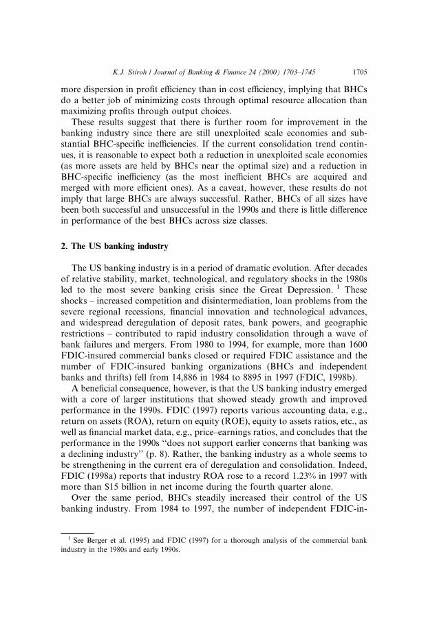
Summary statistics for the sample, Table 1, show trends for 1991±1997that are very similar to the trends for the aggregate industry±increasing meanassets, rising variable pro®ts (de®ned below), and improved ROA (net incomeover assets). Mean variable costs (de®ned below) have also been rising inabsolute terms as the sample increased in average size, but mean variablecosts per total assets (C/A) declined rapidly for 1991±1994 and then stabilizedat a slightly higher level through 1997. Mean ROA and ROE showed asimilar pattern with larger increases from 1991±1993 and small gains for1994±1997.

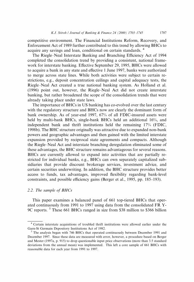
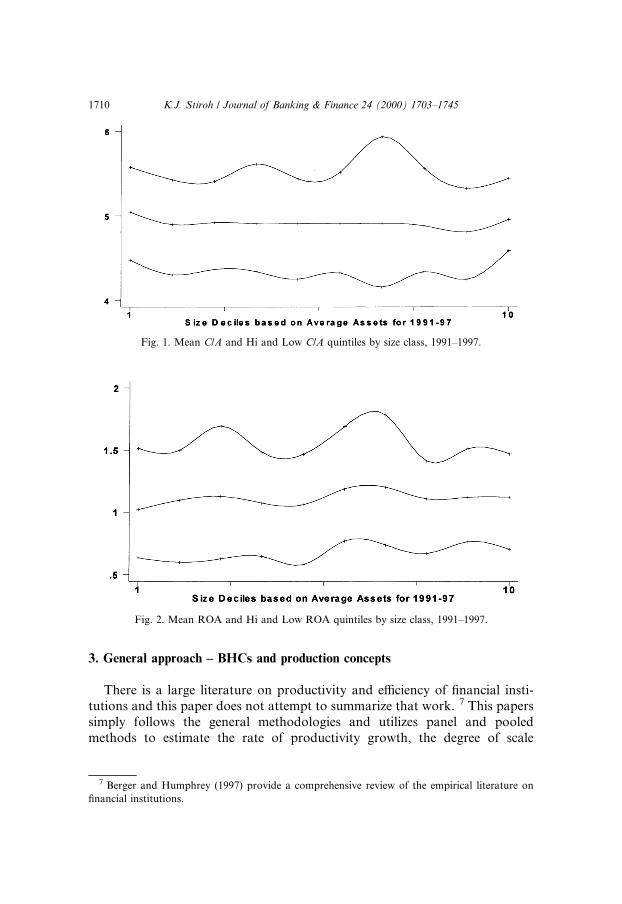
Simply looking at overall means, however, can be misleading and hidessubstantial variation in the performance of individual BHCs. This sample, forexample, covers a wide range of sizes, product mixes, and risk pro®les and allBHCs need not show the same average costs or returns to remain competitive.Large BHCs, for example, hold a di�erent mix of assets with more businessloans and fewer consumer loans. To examine these di�erences, the 661 BHCswere broken down into 10 groups based on average assets for 1991±1997 toensure roughly comparable product mixes. Each asset class was then furtherdecomposed into quintiles based on either average C/A or average ROA for1991±1997 to explore the dispersion of performance both across and within sizeclasses.

Fig. 1 graphs the mean C/A for the highest quintile, the entire size class, andthe lowest quintile for each size class, while Fig. 2 shows the same breakdownfor ROA. 6 These charts show wide dispersion within every size class for bothC/A and ROA, with a slight trend towards lower C/A for larger size classes,except for the very largest BHCs, which show an increase in C/A. There is alsoa small upward trend in ROA for large BHCs and a narrowing of the ROAdistribution within the largest size classes. These data show substantial varia-tion in performance and are suggestive of some scale economies for BHCs. Thequestion of economies of scale and more precise estimates of relative perfor-mance are addressed in the following sections.

6 Berger and Humphrey (1992) report substantial dispersion in costs per asset for commercial

banks in the 1980s.


Ta

ble

1

Tre

nd

sin

ba

nk

ho

ldin

gco

mp

an

yp

erfo

rma

nce

,1

99

1±1997

a

Yea

rN

um

ber

of

Ob

s.

To

tal

ass

ets

Eq

uit

y

cap

ita

l

Vari

ab

le

cost

s

Vari

ab

lep

ro®

tsR

OA

RO

EC

/A

P-1

an

d

P-4

P-2

P-3

19

91

66

12

79

7.8

19

1.4

177.4

54.3

89.5

57.6

0.8

01

0.4

36.2

5

19

92

66

13

09

7.6

23

4.9

147.9

66.6

106.7

70.3

1.0

413.3

04.9

6

19

93

66

13

35

7.8

26

7.9

138.5

70.3

116.2

74.8

1.1

413.7

54.3

1

19

94

66

13

69

2.8

28

5.3

158.4

74.9

122.6

78.2

1.1

313.3

84.2

9

19

95

66

14

13

0.1

33

1.8

211.4

80.3

135.9

84.1

1.1

713.3

14.8

8

19

96

66

14

72

8.1

38

7.7

233.9

91.9

162.7

96.9

1.2

313.5

94.8

4

19

97

66

15

30

3.6

42

7.4

261.6

98.4

182.1

104.1

1.2

413.6

44.8

9

aA

llv

alu

esa

resi

mp

lem

ean

s.V

ari

ab

leco

sts

an

dv

ari

ab

lep

ro®

tsare

de®

ned

inS

ecti

on

3.3

.T

ota

lass

ets,

equ

ity

cap

ital,

vari

ab

leco

sts,

an

dvari

ab

le

pro

®ts

are

mea

sure

din

mil

lio

ns

of

19

97

do

lla

rs.

RO

Ais

net

inco

me

div

ided

by

aver

age

ass

ets.

RO

Eis

net

inco

me

div

ided

by

aver

age

equ

ity.

C/A

is

va

ria

ble

cost

sd

ivid

edb

yto

tal

ass

ets.

RO

A,

RO

E,

an

dC

/Aare

per

cen

tages

.


3. General approach ± BHCs and production concepts

There is a large literature on productivity and e�ciency of ®nancial insti-tutions and this paper does not attempt to summarize that work. 7 This paperssimply follows the general methodologies and utilizes panel and pooledmethods to estimate the rate of productivity growth, the degree of scale

Fig. 2. Mean ROA and Hi and Low ROA quintiles by size class, 1991±1997.

Fig. 1. Mean C/A and Hi and Low C/A quintiles by size class, 1991±1997.

7 Berger and Humphrey (1997) provide a comprehensive review of the empirical literature on

®nancial institutions.


economies, and the relative e�ciency of BHCs in the 1990s. Berger et al. (1987)and Jagtiani and Khanthavit (1996) provide a framework for estimating scaleeconomies; Berger and Mester (1997b) for productivity growth; Bauer et al.(1998), Berger and Mester (1997a), and Berger et al. (1993) for cost and pro®te�ciency; and Berger and Humphrey (1997, 1992) provide a general discussionon interpretation and methodology.

3.1. Analyzing BHCs

This focus on BHCs is in contrast to much recent work that examines thebehavior of individual commercial banks, e.g., Berger and Mester (1997a,b),Humphrey and Pulley (1997), Jagtiani and Khanthavit (1996), and Berger andHumphrey (1992), although there has been some work on BHCs. Akhaveinet al. (1997) use BHC data to analyze the impact of large mergers on e�ciency;Rivard and Thomas (1997) examine the impact of interstate banking on pro®tvolatility for 218 BHCs in the 1980s; Roland (1997) examines pro®t persistencein 237 BHCs; and Hughes et al. (1996) examine e�ciency and risk for 443BHCs in 1994. This paper presents, as far as is known, the ®rst comprehensiveanalysis of productivity and frontier e�ciency of BHCs in the 1990s. 8

The use of BHC data rather than individual bank data, however, presents atrade-o�. On the advantage side, bank managers, particularly in the 1990senvironment of rapid consolidation, presumably care about the performance ofthe institution as a whole, rather than the individual subsidiary banks. Bergeret al. (1995) conclude that ``looking at the holding company rather than at anindividual bank within an MBHC (multi-bank holding company) may give amore accurate description of the relevant economic entity'' (p. 66) since im-portant business decisions are typically made at the holding company level,holding company a�liates often exchange portfolio items, and the currentregulatory structure e�ectively makes the holding company the risk-manage-ment unit. Akhavein et al. (1997, p. 18) argue that managers will coordinateactivities and optimize production choices with respect to the overall institu-tion. Finally, since the majority of previous research, particularly frontier ef-®ciency studies, analyze individual commercial banks it is worthwhile tocompare the results of analysis at higher levels of business organization.

On the other hand, if input and output choices are actually made at the levelof the individual subsidiary, the holding company data would be less mean-ingful. Nonetheless, the more aggregated BHC seems to be the proper unit ofanalysis and it is important to examine the performance of BHCs in todayÕsevolving banking environment.

8 Other earlier research that examines BHCs includes Grabowski et al. (1993) and Newman and

Shrieves (1993).


3.2. Cost and pro®t functions

The basic econometric analysis examines a variable cost and a variablepro®t function for the sample of 661 BHCs. These two approaches are stan-dard in the literature on ®nancial institutions and are brie¯y described below.In particular, this analysis follows the `ìntermediation'' or `àsset'' approach ofSealey and Lindley (1977) where ®nancial institutions transform deposits andpurchased funds into loans and other assets.

A general variable cost function is

C � f �p; y; z; m; l; ec; t�; �1�where variable costs, C, depend on a vector of input prices, p, a vector ofvariable output quantities, y, a vector of ®xed netputs (either inputs or out-puts), z, a vector of environmental variables, m, BHC-speci®c cost ine�ciency,l, random error, �c, and time, t, which proxies for productivity growth.

Likewise, one can examine the relationship between variable pro®ts, P, andthe same set of explanatory variables with a general variable pro®t function as

P � f �p; y; z; m; p; eP; t�; �2�where p is BHC-speci®c pro®t e�ciency and eP is a random error term.

There are several important things to note about Eqs. (1) and (2). First, coste�ciency and pro®t e�ciency need not be the same since a BHC, for example,can e�ciently choose inputs, yet make errors and be ine�cient in the choice ofoutputs. Berger and Mester (1997a), for example, ®nd cost and pro®t e�ciencyto be negatively related and Akhavien et al. (1997) report that mergers improvepro®t e�ciency, but not cost e�ciency. Thus, this paper examines bothmeasures.

Second, Eq. 2 is an `àlternative'' pro®t function that relates pro®ts toquantities of outputs, rather than a ``standard'' pro®t function that relatespro®ts to prices of outputs. Humphrey and Pulley (1997) derive this type ofalternative pro®t function from a bankÕs pro®t maximization problem in thepresence of market power in the output market and review the empirical evi-dence for this assumption. Since these assumptions are reasonable for BHCsand both types of pro®t functions led to similar results with this sample, onlythe results from the alternative pro®t function are reported here. Moreover,di�culties in estimating prices for some assets make the alternative pro®tfunction more attractive. 9

9 Berger and Mester (1997a) present several additional arguments why the alternative pro®t

function may be preferable, e.g., quality di�erences, semi-®xed outputs, imperfect markets, and

large errors in price measurement.


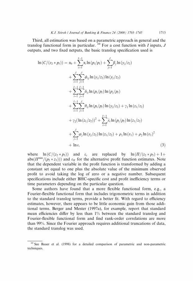
Third, all estimation was based on a parametric approach in general and thetranslog functional form in particular. 10 For a cost function with I inputs, Joutputs, and two ®xed netputs, the basic translog speci®cation used is

ln�C=�z2 � pI�� a0 �XIÿ1

i�1

ai ln�pi=pI� �XJ

j�1

bj ln�yj=z2�

�XJ

i�1

XJ

j�1

/ij ln�yj=z2� ln�yj=z2�

�XIÿ1

i�1

XIÿ1

j�1

dij ln�pi=pI� ln�pj=pI�

�XIÿ1

i�1

XJ

j�1

hij ln�pi=pI� ln�yj=z2� � c1 ln�z1=z2�

� c2� ln�z1=z2��2 �XIÿ1

i�1

ki ln�pi=pI� ln�z1=z2�

�XJ

j�1

uj ln�yj=z2� ln�z1=z2� � q1 ln�v1� � q2 ln�v1�2

� lne; �3�

where ln�C=�z2 � p3�� and ec are replaced by ln�P=�z2 � p3� � 1�abs�Pmin=�p2 � z3�� and eP for the alternative pro®t function estimates. Notethat the dependent variable in the pro®t function is transformed by adding aconstant set equal to one plus the absolute value of the minimum observedpro®t to avoid taking the log of zero or a negative number. Subsequentspeci®cations include either BHC-speci®c cost and pro®t ine�ciency terms ortime parameters depending on the particular question.

Some authors have found that a more ¯exible functional form, e.g., aFourier-¯exible functional form that includes trigonometric terms in additionto the standard translog terms, provide a better ®t. With regard to e�ciencyestimates, however, there appears to be little economic gain from those addi-tional terms. Berger and Mester (1997a), for example, report that standardmean e�ciencies di�er by less than 1% between the standard translog andFourier-¯exible functional form and ®nd rank-order correlations are morethan 99%. Since the Fourier approach requires additional truncations of data,the standard translog was used.

10 See Bauer et al. (1998) for a detailed comparison of parametric and non-parametric

techniques.


Finally, standard restrictions and transformations were incorporated to beconsistent with economic theory. Costs, pro®ts, and all input prices are scaledby one arbitrarily chosen input price (pI ) to impose linear homogeneity.Symmetry restrictions in the quadratic terms (/ij � /ji and dij � dji) of the costand pro®t functions are also imposed. Costs, pro®ts, and all quantities (vari-able outputs and ®xed netputs) are scaled by one ®xed netput, chosen as equitycapital, to control for heteroskedasticity and reduce the scale bias that resultsfrom including BHCs of very di�erent sizes in a single regression. That is,scaling by equity capital makes both the cost and pro®t dependent variables inthe same range for all institutions. 11

3.3. Variable de®nitions

An important decision in this analysis is the speci®cation of outputs andinputs. In the asset approach, ®nancial assets are treated as outputs and ®-nancial liabilities and physical factors are the inputs. Since there is somequestion about which variables to include, this analysis generally follows thevariable de®nitions and speci®cations of the ``preferred model'' in Berger andMester (1997a). One important departure, however, is the treatment of non-traditional outputs, which is discussed in detail below. Table 2 provides sum-mary statistics for the variables used in the cost and pro®t functions. Allvariables are measured in 1997 dollars.

On the input side, three inputs are included. The price vector, p, includes theinterest rate on purchased funds (jumbo certi®cates of deposits (CDs), federalfunds purchased, and liabilities except core deposits), the interest rate on coredeposits (domestic deposits less jumbo CDs), and the price of labor. This isconsistent with Akhavein et al. (1997), who include total deposit funds (in-cluding purchased funds) and labor as the inputs, and follows Berger andMester (1997a).

On the output side, things are less clear since BHCs do much more than``traditional'' banking activities like making loans and holding securities as inthe standard speci®cation. BHCs earn a substantial portion of revenue from feeand service activities and OBS items like lines of credit, loan commitments, andderivatives are now important activities. Since these ``non-traditional'' activi-ties are growing over time and concentrated in the largest institutions, failure toaccount for them may lead to incorrect conclusions.

11 Berger and Mester (1997a, p. 918) discuss this transformation and the economic interpretation

of scaling by equity capital. Note also that predicted costs and pro®ts are calculated by

exponentiating the ®tted value from the log speci®cation and then multiplying by the scaling

factors. Since this adjustment is non-linear, average predicted values are multiplicatively adjusted to

equal actual mean values when needed.


One set of non-traditional activities includes the sources of non-interestincome, e.g., ®duciary activities, trading, and activities that generate other non-interest income like fee income from credit cards, mortgage servicing, mutualfund and annuity fees, and ATM surcharges. According to English and Nelson(1998), non-interest income has increased from 26% to 38% of total bankrevenue since the mid-1980s as the bank product set expands. OBS items likeloan commitments, letters of credit, derivatives, and loan securitization areanother type of non-traditional activity that is increasing in importance. 12

These items in particular are highly concentrated in the largest institutions,e.g., Berger et al. (1995) report that the notional value of derivatives was 11.5

Table 2

Cost and pro®t function variables, 1997a

Mean S.D. Minimum Maximum

Variable costs 261.6 1212.4 1.8 19,035.0

Variable pro®ts

P-1 and P-4 98.4 394.2 )89.0 4,958.0

P-2 182.1 827.1 1.1 1,007.0

P-3 104.1 434.1 )41.7 5,650.0

Variable input prices

Purchased funds 4.68 0.77 0.03 8.99

Core deposits 3.29 0.59 1.00 4.89

Labor 37.70 7.73 3.79 78.76

Variable output quantities

Business loans 572.2 2609.7 0.3 33,431.0

Consumer loans 2774.1 11,674.3 15.2 143,403.0

Securities 1877.5 10,268.5 18.9 193,287.0

Net non-interest income (Y-2) 83.7 466.7 0.6 7937.2

O�-balance sheet items (Y-3) 840.1 6730.9 0.1 137,607.1

Fixed netputs

Physical capital 79.8 340.5 0.1 4147.9

Equity capital 427.5 1807.4 5.0 21,742.0

O�-balance sheet items (Y-4) 840.1 6730.9 0.1 137,607.1

Total assets 5303.6 24,205.9 37.6 365,520.9

a Variable costs, variable pro®ts, variable output quantities, ®xed netputs, and total assets are

measured in millions of 1997 dollars. Price of purchased funds and core deposits are percentages.

Price of labor is in thousands of 1997 dollars. Speci®cation Y-1 includes business loans, consumer

loans, and securities as outputs and physical capital and equity capital as ®xed netputs. Other

speci®cations include Y-1 plus the designated output quantity or ®xed netput.

12 See English and Nelson (1998) for a discussion of the importance of di�erent types of

o�-balance sheet items.


times assets for megabanks (BHCs with more than $100 billion in assets in1994) and only 0.002 times assets for small banks (BHCs and banks with lessthan $100 million in assets in 1994).

These non-traditional activities are clearly increasing in importance, but thewide range of activities and imperfect data make analysis problematic. Forexample, it is straightforward to calculate the credit equivalent dollar value ofOBS items from regulatory data, but it is di�cult to consistently estimate theassociated revenue for a pro®t function analysis. Nonetheless, there have re-cently been several innovative attempts to account for non-traditional activitiesin cost and pro®t function analysis.

Rogers (1998) uses the revenue from non-traditional activities, de®ned as``net non-interest income'', equal to total non-interest income less servicecharges earned on deposits, as a proxy for both the quantity and the revenueassociated with non-traditional activities. Berger and Mester (1997a) cite theproblems with estimating revenue from OBS items and include risk-weightedOBS items as a ®xed netput in both a cost and pro®t estimation. Jagtiani andKhanthavit (1996) estimate a cost function only, and thus avoid problematicrevenue estimates, and include the risk-weighted, credit equivalent of OBSproducts as an output.

Since each of these approaches is imperfect, this paper de®nes and comparesfour alternative speci®cations. The ®rst speci®cation, Y-1, includes only tra-ditional measures of bank outputs and de®nes the variable output vector toinclude three outputs ± business loans, consumer loans, and securities (all as-sets except loans and physical capital). The second, Y-2, uses RogersÕ (1998)de®nition and expands the output vector to include net non-interest income(total non-interest income less service charges on deposits) as a fourth output.A third speci®cation, Y-3, follows Jagtiani et al. (1995) and includes the creditequivalent of OBS items (loan commitments, credit derivatives, foreign ex-change and interest rate contracts) as a fourth output. 13 The ®nal speci®ca-tion, Y-4, follows Berger and Mester (1997a) and uses the three traditionaloutputs, but includes the credit equivalent of OBS items as a ®xed netput z. Theother ®xed netputs, in all cases, include premises and ®xed assets, and totalequity capital.

From these inputs and outputs, variable costs, C, and variable pro®ts, P,are de®ned as follows. For all speci®cations, variable costs are the interest

13 The credit equivalent of o�-balance sheet items are reported by risk category in Part II of

schedule HC-I of the FR Y-9C report. The transformation to credit equivalent values is described

in the Federal Reserve BoardÕs Capital Adequacy Guidelines for Bank Holding Companies. For

example, direct credit substitutes are converted at 100%, transaction related contingencies are

converted at 50%, and short-term, self-liquidating, trade-related contingencies are converted at

20%. If a BHC does not have all of these items, the minimum value of the credit equivalent sum for

each year is assigned to prevent taking logs of a zero value.


expense on purchased funds and on core deposits plus total salary and bene®tsexpenditure. Variable pro®ts, however, depend on the output speci®cation. Forthe ®rst speci®cation of output, variable pro®ts, P-1, are de®ned as interestincome from all loans and securities less the variable costs. P-2 augments P-1with net non-interest income de®ned above. P-3 augments P-1 with total OBStrading income plus the impact on income from OBS derivatives held forpurposes other than trading. 14 Prior to 1995, however, these revenue itemswere not required to be reported so trading income, which equals only thetrading portion, was used. P-4 is equal to P-1 since the OBS items are treatedas a ®xed netput and thus do not have an associated revenue stream. 15

As mentioned above, each speci®cation has certain weaknesses so it is usefulto estimate all forms and examine the robustness of the results. Y-1 su�ers sinceit totally excludes non-traditional activities, which are growing and concen-trated in large BHCs. Y-2 is imperfect since it treats the revenue and thequantity of non-traditional activities as identical and does not account for pricevariation. Y-3 is a good speci®cation for the cost function, but is less reliablefor the pro®t function due to the changing de®nition and imprecise revenueestimates for OBS items. Y-4 does not require revenue from OBS items, whichis an advantage, but it treats OBS items as ®xed and thus a�ects the estimatesof scale economies. Despite these limitations, a comparison of results acrossspeci®cations should lead to a robust view of the behavior of BHCs in the1990s.

4. Productivity growth in the 1990s

Table 1 shows that these BHCs improved their performance in the 1990s asmean ROA increased and mean C/A declined. A possible source of improve-ment is productivity growth, measured as a shift in the cost function, whichlowers costs for a given set of input prices, output quantities, and other ex-planatory variables.

This section uses three related econometric methodologies to estimate ratesof productivity growth in the 1990s. The ®rst approach simply pools the annualdata into a single regression and estimates the shift in a common cost function.The second approach, following Lang and Welzel (1996), uses panel datamethods to incorporate BHC-speci®c e�ects and again measures how the costfunction shifts over time. The ®nal approach, based on Berger and Mester

14 These items are included as memorandum items M9-M10 of Schedule HI on the FR Y-9C

report.15 Note that both net non-interest income and OBS items cannot be included in the same

regression since the associated revenues overlap.


(1997b), decomposes total cost changes into a portion due to changes inbusiness conditions and a portion due to changes in BHC productivity.

Each productivity method is estimated using the four alternative outputspeci®cations, Y-1±Y-4. When applying these approaches with the translog costfunction, however, it does not matter if a variable is labeled an output or a®xed netput, so speci®cation Y-3 and Y-4 yield identical productivity results.Thus, results for only three output speci®cations are reported. Results from thethree econometric methods yield a rate of productivity growth in the range of0.4% for the 1990s and suggest that productivity growth played a role in theimproved performance during the 1990s.

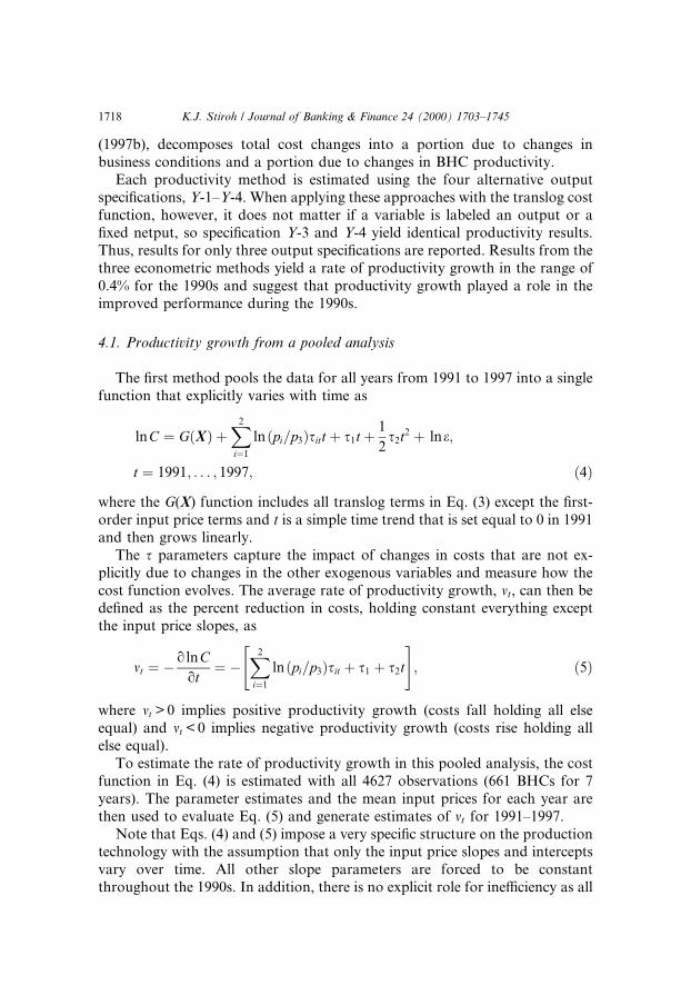
4.1. Productivity growth from a pooled analysis

The ®rst method pools the data for all years from 1991 to 1997 into a singlefunction that explicitly varies with time as

lnC � G�X� �X2

i�1

ln�pi=p3�sitt � s1t � 1

2s2t2 � lne;

t � 1991; . . . ; 1997; �4�where the G(X) function includes all translog terms in Eq. (3) except the ®rst-order input price terms and t is a simple time trend that is set equal to 0 in 1991and then grows linearly.

The s parameters capture the impact of changes in costs that are not ex-plicitly due to changes in the other exogenous variables and measure how thecost function evolves. The average rate of productivity growth, mt, can then bede®ned as the percent reduction in costs, holding constant everything exceptthe input price slopes, as

mt � ÿ o lnCot� ÿ

X2

i�1

ln�pi=p3�sit

"� s1 � s2t

#; �5�

where mt > 0 implies positive productivity growth (costs fall holding all elseequal) and mt < 0 implies negative productivity growth (costs rise holding allelse equal).

To estimate the rate of productivity growth in this pooled analysis, the costfunction in Eq. (4) is estimated with all 4627 observations (661 BHCs for 7years). The parameter estimates and the mean input prices for each year arethen used to evaluate Eq. (5) and generate estimates of mt for 1991±1997.

Note that Eqs. (4) and (5) impose a very speci®c structure on the productiontechnology with the assumption that only the input price slopes and interceptsvary over time. All other slope parameters are forced to be constantthroughout the 1990s. In addition, there is no explicit role for ine�ciency as all


BHCs are implicitly assumed to operate on a single cost frontier. This is clearlya restrictive speci®cation and the next two subsections generalize this.

4.2. Productivity growth from a panel analysis

A more general approach augments the pooled speci®cation in Eq. (4) withBHC-speci®c intercepts through a BHC-speci®c e�ect, ai, as

lnC � G�X� � ai �X2

i�1

ln�pi=p3�sitt � s1t � 1

2s2t2 � lne;

t � 1991; . . . ; 1997: �6�

Eq. (6) maintains the assumptions that slopes coe�cients, except for the®rst-order input price terms, are constant throughout the 1990s, but generalizesEq. (4) by recognizing persistent cost di�erences through ai, which raise costsall else equal. This unobserved term accounts for all di�erences ± location,management skills, or persistent X-ine�ciency ± that permanently raise thevariable costs of a particular BHC relative to other BHCs that face similarconditions. 16 Berger (1993) discusses the potential bias in scale economy es-timates if the unobserved variable is correlated to cost function regressors. Forexample, if X-e�cient BHCs grow large, then the impact of e�ciency may bemislabeled as the impact of scale economies.

An econometric issue in this type of speci®cation is how to interpret andestimate the ai terms. If ai is a ®xed parameter for each BHC that simply shiftsthe common cost function, then a ``®xed e�ects'' methodology is appropriateand ai can be estimated like any other parameter. 17 That is, persistent di�er-ences across BHCs are re¯ected in di�erences in the intercepts, which representthe unobserved e�ects. This approach assumes that the ai are non-random, butcorrelated with the independent variables. Since the ®xed-e�ects are assumed tobe permanent characteristics, strictly speaking, the results only apply to thissample and do not generalize to other BHCs. A ``random e�ects'' methodol-ogy, on the other hand, views ai as a random, though permanent, variable thatis drawn from a distribution and assumes that ai is uncorrelated with the otherexplanatory variables. Under this interpretation, the sample is viewed as rep-resentative of the entire population and statistical inference is possible. Since itis unclear a priori which approach is correct, both are used and speci®cationtests are reported along with the empirical results. 18

16 The issue of ine�ciency is dealt with in more detail in Section 4.17 The ®xed e�ect estimator is equivalent to a ``within estimator'' from an ordinary least squares

regression of deviations from the mean for each BHC.18 See Chamberlain (1984) for details.


Estimates of productivity growth are then calculated in the same way as inthe pooled analysis. A single regression with 4627 observations is used toestimate the generalized cost function in Eq. (6) using both the ®xed e�ect orthe random e�ect methodology. The estimated parameters are then combinedwith mean values each year to generate two alternative estimates of pro-ductivity growth, mfe

t and mret , for the ®xed and random e�ect methodologies,

respectively.

4.3. Productivity growth from a cost decomposition

The ®nal approach begins with the observation that costs rise if BHCseither face less favorable economic conditions, e.g., an increase in inputprices, or if they become less productive in their operations. One can employthe cost framework to decompose observed cost changes into these twofactors as

Total cost change � ft�1�X t�1�ft�X t� �

ft�1�X t�ft�1�X t� �

ft�1�X t�ft�X t� ; �7�

where Xt represents all components of the cost function in Eq. (3) and ft��represents the cost function available to BHCs, both at time t.

The ®rst term on the right-hand side of Eq. (7) represents the changein costs that result from the change in economic conditions, e.g., changesin Xt to Xt� 1, for a given cost function, ft�1��. The second term rep-resents the change in cost that result from a change in the cost function,ft�� to ft�1��, holding economic conditions constant at Xt. Thus, the ®rstterm captures the impact of changing business conditions, while the sec-ond term captures the impact of changing production techniques orproductivity.

To implement this approach, parameter estimates from a separate costfunction regression for each year between 1991 and 1997 are used to estimateft�1�� and ft��. The mean value of each variable in Eq. (3) for all BHCs ineach year was then used for Xt� 1 and Xt. By combining the parameter esti-mates and mean values for di�erent annual periods, one can calculate eachelement in the cost decomposition in Eq. (7).

4.4. Estimates of productivity growth

Table 3 reports the estimated annual rate of productivity growth for theentire period 1991±97 for the four methods described above ± pooled data,®xed e�ects, random e�ects, and cost decomposition ± for each of three outputspeci®cations. The estimates are very close, typically falling between 0.31% and0.59% per year. An obvious outlier, however, is the cost decomposition for theY-2 speci®cation. The annual point estimates and standard errors for each


econometric method and each output speci®cation are reported in Tables 3a±c. 19 Results for the Y-4 speci®cation, which is similar to other speci®cations, isgraphed in Fig. 3.

It should be made clear that these estimates of productivity growth corre-spond to multi-factor productivity. That is, the econometric approach controlsfor changes in inputs and output size, so mt measures the shift in the cost

Table 3

Average productivity growth rates, 1991±1997a

Output speci®cation Pooled

analysis

Fixed

e�ects

Random

e�ects

Cost

decomposition

Y-1: business loans, consumer loans,

securities

0.44 0.47 0.45 0.32

Y-2: business loans, consumer loans,

securities,

net non-interest income

0.42 0.50 0.47 0.05

Y-3 and Y-4: business loans, consumer

loans, securities, o�-balance sheet items

as an output or as a ®xed netput

0.44 0.46 0.45 0.31

a All estimates are from cost function regressions for 1991±1997 as a whole. Estimation details are

given in Section 4. All values are percentages and simple means of average annual growth rates.

Table 3a

Annual estimates of productivity growth, 1991±1997,

Y-1: business loans, consumer loans, securitiesa

Year Pooled analysis Fixed e�ect Random e�ect Cost decomposition

1992 0.242 )0.438 )0.302 0.236

(0.225) (0.114) (0.111)

1993 0.596 0.129 0.214 )0.771

(0.177) (0.083) (0.081)

1994 0.614 0.453 0.472 0.016

(0.120) (0.052) (0.051)

1995 0.280 0.529 0.466 1.979

(0.092) (0.049) (0.049)

1996 0.426 0.900 0.781 0.348

(0.164) (0.083) (0.082)

1997 0.473 1.223 1.041 0.089

(0.248) (0.125) (0.124)

Mean 0.438 0.466 0.445 0.316

a Standard errors are in parentheses for the econometric estimates. Estimation details are given in

Section 4. All growth rates are percentages.

19 Note that productivity growth rate from the cost decomposition cannot be estimated for 1991

since that requires actual cost data for 1990. To be consistent, Tables 3a±c report the various

productivity growth rate estimates, mt, from 1992 onward.


function over time. In this context, 0.4% growth is very respectable whencompared to the economy as a whole. BLS (1998), for example, estimatesmulti-factor productivity growth of 0.3% per year for the private businesseconomy and 1.9% for manufacturing for 1990±1996. Since manufacturing is a

Table 3b

Annual estimates of productivity growth, 1991±1997,

Y-2: business loans, consumer loans, securities, net non-interest incomea


1992 )0.683 )0.449 )0.418 )0.802

(0.215) (0.111) (0.109)

1993 0.024 0.139 0.158 )1.784

(0.163) (0.081) (0.079)

1994 0.414 0.479 0.472 )0.741

(0.105) (0.050) (0.050)

1995 0.474 0.563 0.516 2.919

(0.084) (0.048) (0.048)

1996 0.951 0.951 0.886 0.396

(0.151) (0.081) (0.081)

1997 1.351 1.289 1.201 0.334

(0.231) (0.123) (0.122)

Mean 0.422 0.495 0.469 0.054



Table 3c

Estimates of productivity growth, 1991±1997,

Y-3 and Y-4: business loans, consumer loans, securities, o�-balance sheet items as an output or as a

®xed netputa


1992 0.219 )0.429 )0.289 0.075

(0.226) (0.114) (0.111)

1993 0.587 0.131 0.221 )0.727

(0.179) (0.083) (0.081)

1994 0.615 0.451 0.475 0.126

(0.122) (0.052) (0.051)

1995 0.288 0.524 0.465 2.005

(0.092) (0.049) (0.049)

1996 0.446 0.890 0.774 0.348

(0.163) (0.083) (0.082)

1997 0.504 1.208 1.029 0.061

(0.247) (0.125) (0.124)

Mean 0.443 0.463 0.446 0.315




substantial share of output, this implies that estimated BHC productivitygrowth far exceeded multi-factor productivity for the non-manufacturingsectors of the US economy.

When comparing the alternative methods, econometric tests strongly rejectthe pooled analysis in favor of a panel approach that incorporates persistent®rm di�erences. An F-test of identical intercepts for all BHCs is rejected at the1% level in the ®xed e�ects model and a Breusch±Pagan test rejects the as-sumption of equal random e�ects at the 1% level in the random e�ects model.A Hausman speci®cation test, however, rejects the null hypothesis that therandom e�ects are uncorrelated with the other right-hand side variables. Thisimplies either that the cost function is misspeci®ed or the assumption of un-correlated random e�ects is violated.

As a whole, these results are quite consistent with the simple ROA and C/Ameans presented in Table 1 since the econometric estimates control for changesin all right-hand side variables, including BHC size. For 1991±1997, for ex-ample, mean costs rose 6.5% per year, but mean BHC size grew even faster asassets increased at 10.7% per year and mean equity (the scaling factor in thecost regressions) increased 13.4% annually. Since these productivity estimatesare derived from predicted changes in costs, ceteris paribus, the relatively slowincrease in costs partially represents real productivity growth.

Fig. 3. Annual productivity growth for alternative econometric methods for Y-3 and Y-4,

1992±1997.


This can also be seen from the details of the cost decomposition from Eq. (7)that are shown in Table 4. For the entire period 1991±1997, the average actualcost increase was 6.47% per year (the weighted average column) while predictedcosts increased 6.99 per year. This predicted cost change is decomposed into a7.0% to 7.3% annual increase due to changing business conditions and a 0.05±0.32% annual decrease due to productivity growth. This implies that had thebusiness and operating environment, e.g., size and input prices, stayed at the

Table 4

Comparison of actual cost change to estimated cost decomposition, 1991±1997a

Year Actual cost change Estimated cost decomposition

Mean Weighted

average

Total cost

change

± of

productivity

growth

Change in

business

conditions

Y-1: Business loans, consumer loans, securities

1991±1992 )17.62 )18.25 )6.95 )0.24 )6.71

1992±1993 )9.32 )6.52 )7.91 0.77 )8.68

1993±1994 5.37 13.41 6.44 )0.02 6.46

1994±1995 20.80 28.87 23.47 )1.98 25.45

1995±1996 7.13 10.09 17.15 )0.35 17.50

1996±1997 9.50 11.22 9.74 )0.09 9.83

Mean 2.64 6.47 6.99 )0.32 7.31

Y-2: Business loans, consumer loans, securities,

net non-interest income

1991±1992 )6.95 0.80 )7.75

1992±1993 )7.91 1.78 )9.69

1993±1994 6.44 0.74 5.70

1994±1995 23.47 )2.92 26.39

1995±1996 17.15 )0.40 17.55

1996±1997 9.74 )0.33 10.08

Mean 6.99 )0.05 7.05

Y-3 and Y-4: Business loans, consumer loans, o�-

balance sheet items

1991±1992 )6.95 )0.08 )6.87

1992±1993 )7.91 0.73 )8.64

1993±1994 6.44 )0.13 6.57

1994±1995 23.47 )2.01 25.48

1995±1996 17.15 )0.35 17.50

1996±1997 9.74 )0.06 9.80

Mean 6.99 )0.31 7.31

a Total cost change is de®ned as ln(ft� 1(Xt� 1)/ft(Xt))�100. ± of productivity growth is de®ned as

ln(ft� 1(Xt)/ft(Xt))�100. Change in business conditions is de®ned as ln(ft� 1(Xt� 1)/ft� 1(Xt))�100. All

growth rates are percentages.


1991 levels, then total costs would have fallen about 2.0% in 1997 relative to1991.

These results show that productivity growth was a source of the improvedperformance of BHCs in the 1990s. The results, however, are quite di�erentfrom Berger and Mester (1997b) who report 10% cost increases per year for1989±1995 after accounting for changes in business conditions. This mightre¯ect the di�erent samples, i.e., relatively large BHCs vs. smaller individualbanks, or the di�erent set of control variables used in each speci®cation.Compared with the raw data that show asset growth of 11% per year and costincrease of 7% per year, however, the ®nding of 0.4% annual productivitygrowth for BHCs seems reasonable.

5. Economies of scale for BHCs in the 1990s

Scale economies ± intuitively described as a decrease in average costs as sizeincreases ± has been an important topic in the empirical study of commercialbanks. Perhaps surprisingly, most early research found little evidence ofeconomies of scale beyond a relatively modest overall size. Recent evidencefrom the 1990s, however, suggests sizable economies of scale that increase withbank size. Hughes and Mester (1998), for example, ®nd the largest quartile ofcommercial banks in 1990 have the largest degree of scale economies, Bergerand Mester (1997a) report that an average bank would have to be 2±3 times aslarge to maximize cost scale e�ciency, and Hughes et al. (1996) ®nd that BHCswith assets greater than $50 billion have the largest degree of scale economiesin 1994. Moreover, Berger and Mester (1997a) test several speci®cationsand conclude ``the 1990s are indeed di�erent'' (p. 928) with regard to scaleeconomies.

This section reports estimates of economies of scale for the BHCs for 1991to 1997. The estimates complement the earlier work of and Hughes and Mester(1998), Berger and Mester (1997a), and Jagtiani and Khanthavit (1996) oncommercial banks rather than BHCs and Hughes et al. (1996), which examinesa smaller subset of BHCs for only 1994. This broader analysis of BHCs allowsan investigation of how scale economies vary across size classes, possiblychanged during the period of deregulation and heavy consolidation in the1990s, and contributed to the success of BHCs in the 1990s.

5.1. Measures of economies of scale

Estimates of the degree of scale economies measure how costs vary withchanges in output and can be calculated from an estimated cost function. SinceBHCs produce many outputs, multi-product equivalents to a cost±outputelasticity have been developed and used in numerous studies. This paper


estimates and reports two well-known measures ± ray scale economies andexpansion path scale economies ± for the sample of BHCs for 1991±1997. Thefour alternative speci®cations, Y-1 through Y-4, are used to estimates eachmeasure.

Ray scale economies (RSE) measures the elasticity of cost with respect to aproportional increase in all outputs and is de®ned as

RSE �XJ

j�1

o lnCo lnyj

; �8�

where yj is the jth output from the y output vector with J assets. RSE < 1implies economies of scale (costs increase proportionally less than output in-creases) and RSE > 1 implies diseconomies of scale.

This de®nition, however, measures the change in costs as a BHC increasesall outputs proportionally. This implicitly assumes the same output mix overall BHC size classes, an assumption that is not consistent with the observedasset portfolios of BHCs. Larger BHCs, for example, hold fewer securities andmore business loans than smaller BHCs.

To avoid this unrealistic assumption, Berger et al. (1987) developed theconcept of expansion path scale economies, EPSCE(yA, yB), which measuresthe proportional change in costs as a bank moves along the observed expansionpath from output bundle yA to output bundle yB where yB is the larger BHC.EPSCE(yA, yB) is de®ned as

EPSCE�yA; yB� �XJ

i�1

o lnCo lnyj

� yBj ÿ yA

j

yBj

" #,CB ÿ CA

CB

� �; �9�

where CB and CA are the mean of the predicted variable costs for the large andthe small BHC, respectively.

EPSCE�yA; yB� < 1 implies scale economies (costs increase proportionallyless than outputs) and EPSCE�yA; yB� > 1 implies scale diseconomies (costsincrease proportionally more than outputs). EPSCE�yA; yB� is a more usefulmeasure of scale economies since it compares the cost change as BHCs increasein size and change their output mix in way that is consistent with the observedbehavioral choices of BHCs.

5.2. Estimates of scale economies

EPSCE(yA, yB) and RSE were calculated from 1991 to 1997 for the 661BHCs across six asset size classes ± Class 1:<$200 million; Class 2: $200±$300million; Class 3: $300±$500 million; Class 4: $500 million±$1 billion; Class 5:$1±$5 billion; Class 6: >$5 billion. Note that the asset classes were de®ned interms of absolute size rather than relative size. Since BHCs grew steadilyduring the 1990s, it is important to compare scale economies at absolute levels


to determine changes in the optimal size. In all cases, the cost function inEq. (3) with each of the four speci®cations was estimated separately for eachyear and the parameter estimates and mean values from each size class wereused to evaluate Eqs. (8) and (9). Note also that since these estimates are basedon a cost function, the same dependent variable is in each regression regardlessof the output speci®cation.

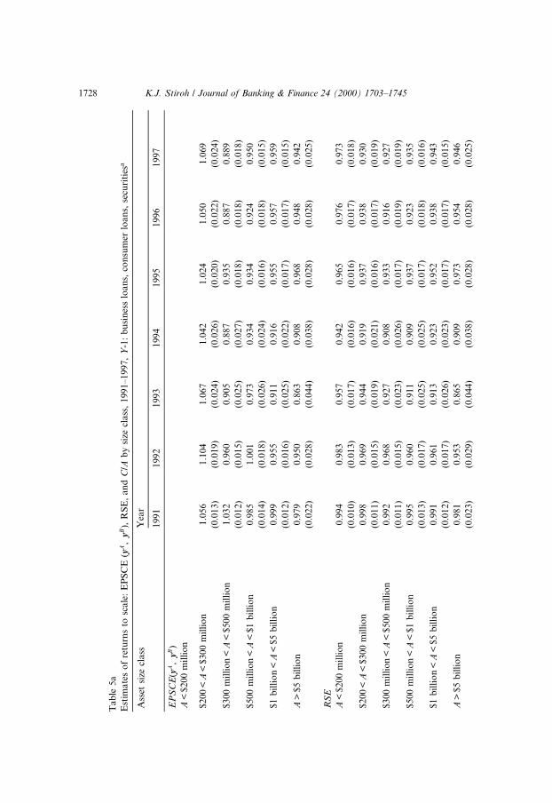
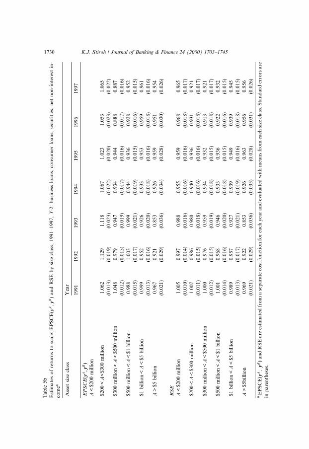
The scale economy results, along with mean C/A for each group, are re-ported in Tables 5a, b, c, d. The estimates are very similar across the fourspeci®cations with modest economies of scale during the 1990s, i.e., the ma-jority of EPSCE(yA, yB) and RSE estimates are signi®cantly below 1.0. The$200m to $300m group is an exception with signi®cant EPSCE(yA, yB) dis-economies of scale for all years.

The degree of scale economies is typically stronger for the largest BHCs,especially using the preferred EPSCE(yA, yB) measure, and there is a de®nitedownward trend in both EPSCE(yA, yB) and RSE in the early 1990s and anincrease thereafter. Both of these ®ndings are consistent with the raw data onC/A and ROA presented earlier. Table 1, for example, shows C/A decliningfrom 1991 to 1994 and mean ROA rising throughout the 1990s, while Figs. 1and 2 show a slight decline in C/A and a small upward trend in ROA acrosssize classes in 1997.

The ®nding that larger banks show more unexploited scale economies isperhaps surprising, but consistent with recent research that found signi®cantscale economies in the 1990s, e.g., Hughes and Mester (1998), Berger andMester (1997a), Hughes et al. (1996), and Jagtiani and Khanthavit (1996).These results also suggest that the optimal scale of BHCs increased in theearly 1990s and then stabilized. From 1991 to 1994, mean BHC size grewsteadily while unexploited scale economies increased, which implies that op-timal size must have been increasing. After 1994, BHCs continued to grow,but there was a decrease in the degree of unexploited scale economies as thecontinued growth during the mid-1990s moved the BHCs closer to the newoptimal size and left less potential gains from unrealized scale economies.Both of these results likely re¯ect the impact of deregulation, e.g., interstatebanking and expanded bank powers, and technological advances, e.g., in-formation and communications equipment, that improved the relative posi-tion of large BHCs.

Finally, the similarity across the four speci®cations is consistent with priorresearch, e.g., Jagtiani et al. (1995) found that OBS activities had a minimalimpact on scale and product mix economies from a cost function analysis,and could represent several factors. Since many BHCs have little in terms ofthese non-traditional outputs, there may not be enough additional variationin the output vector. Speci®cations Y-3 and Y-4 in particular are expected tobe similar since the explanatory variables on the cost regression are identicaland the only di�erence is that change in OBS items is incorporated in the


Ta

ble

5a

Est

imate

so

fre

turn

sto

scale

:E

PS

CE

(yA,

yB),

RS

E,

an

dC

/Ab

ysi

zecl

ass

,1991±1997,

Y-1

:b

usi

nes

slo

an

s,co

nsu

mer

loan

s,se

curi

ties

a

Ass

etsi

zecl

ass

Yea

r

19

91

1992

1993

1994

1995

1996

1997

EP

SC

E(y

A,

yB)

A<

$2

00

mil

lio

n

$2

00

<A

<$

300

mil

lio

n1

.05

61.1

04

1.0

67

1.0

42

1.0

24

1.0

50

1.0

69

(0.0

13

)(0

.019)

(0.0

24)

(0.0

26)

(0.0

20)

(0.0

22)

(0.0

24)

$3

00

mil

lio

n<

A<

$5

00

mil

lio

n1

.03

20.9

60

0.9

05

0.8

87

0.9

35

0.8

87

0.8

89

(0.0

12

)(0

.015)

(0.0

25)

(0.0

27)

(0.0

18)

(0.0

18)

(0.0

18)

$5

00

mil

lio

n<

A<

$1

bil

lio

n0

.98

51.0

01

0.9

73

0.9

34

0.9

34

0.9

24

0.9

50

(0.0

14

)(0

.018)

(0.0

26)

(0.0

24)

(0.0

16)

(0.0

18)

(0.0

15)

$1

bil

lio

n<

A<

$5

bil

lio

n0

.99

90.9

55

0.9

11

0.9

16

0.9

55

0.9

57

0.9

59

(0.0

12

)(0

.016)

(0.0

25)

(0.0

22)

(0.0

17)

(0.0

17)

(0.0

15)

A>

$5

bil

lio

n0

.97

90.9

50

0.8

63

0.9

08

0.9

68

0.9

48

0.9

42

(0.0

22

)(0

.028)

(0.0

44)

(0.0

38)

(0.0

28)

(0.0

28)

(0.0

25)

RS

E

A<

$2

00

mil

lio

n0

.99

40.9

83

0.9

57

0.9

42

0.9

65

0.9

76

0.9

73

(0.0

10

)(0

.013)

(0.0

17)

(0.0

16)

(0.0

16)

(0.0

17)

(0.0

18)

$2

00

<A

<$

300

mil

lio

n0

.99

80.9

69

0.9

44

0.9

19

0.9

37

0.9

38

0.9

30

(0.0

11

)(0

.015)

(0.0

19)

(0.0

21)

(0.0

16)

(0.0

17)

(0.0

19)

$3

00

mil

lio

n<

A<

$5

00

mil

lio

n0

.99

20.9

68

0.9

27

0.9

08

0.9

33

0.9

16

0.9

27

(0.0

11

)(0

.015)

(0.0

23)

(0.0

26)

(0.0

17)

(0.0

19)

(0.0

19)

$5

00

mil

lio

n<

A<

$1

bil

lio

n0

.99

50.9

60

0.9

11

0.9

09

0.9

37

0.9

23

0.9

35

(0.0

13

)(0

.017)

(0.0

25)

(0.0

25)

(0.0

17)

(0.0

18)

(0.0

16)

$1

bil

lio

n<

A<

$5

bil

lio

n0

.99

10.9

61

0.9

13

0.9

23

0.9

52

0.9

38

0.9

43

(0.0

12

)(0

.017)

(0.0

26)

(0.0

23)

(0.0

17)

(0.0

17)

(0.0

15)

A>

$5

bil

lio

n0

.98

10.9

53

0.8

65

0.9

09

0.9

73

0.9

54

0.9

46

(0.0

23

)(0

.029)

(0.0

44)

(0.0

38)

(0.0

28)

(0.0

28)

(0.0

25)


C/A

A<

$2

00

mil

lio

n6

.29

5.1

24.4

24.4

24.9

95.0

15.0

3

(0.5

2)

(0.4

6)

(0.4

9)

(0.4

0)

(0.4

2)

(0.4

5)

(0.4

2)

$2

00

<A

<$

300

mil

lio

n6

.32

4.9

94.3

44.2

54.8

44.8

24.8

9

(0.5

5)

(0.5

5)

(0.4

8)

(0.4

3)

(0.4

7)

(0.4

4)

(0.4

4)

$3

00

mil

lio

n<

A<

$5

00

mil

lio

n6

.16

4.9

84.4

24.3

44.8

44.8

14.8

9

(0.7

1)

(0.8

9)

(0.9

7)

(0.9

2)

(0.5

0)

(0.4

9)

(0.5

3)

$5

00

mil

lio

n<

A<

$1

bil

lio

n6

.20

4.8

34.1

44.1

84.8

74.8

54.8

9

(0.6

0)

(0.5

2)

(0.4

6)

(0.4

7)

(0.9

0)

(0.8

3)

(0.7

7)

$1

bil

lio

n<

A<

$5

bil

lio

n6

.19

4.9

04.2

74.2

24.8

24.7

54.8

1

(0.5

3)

(0.4

4)

(0.6

3)

(0.4

8)

(0.5

5)

(0.6

2)

(0.5

5)

A>

$5

bil

lio

n6

.25

4.8

44.2

04.3

55.1

14.9

44.8

9

(0.4

8)

(0.4

0)

(0.4

3)

(0.4

2)

(0.4

6)

(0.5

1)

(0.5

1)

aE

PS

CE

(yA,

yB)

an

dR

SE

are

esti

ma

ted

fro

ma

sep

ara

teco

stfu

nct

ion

for

each

yea

ran

dev

alu

ate

dw

ith

mea

ns

fro

mea

chsi

zecl

ass

.S

tan

dard

erro

rsare

inp

are

nth

eses

.C

/Ais

va

riab

leco

sts

per

ass

ets

mu

ltip

lied

by

100

an

dth

est

an

dard

dev

iati

on

for

each

size

class

isin

pare

nth

eses

.


Ta

ble

5b

Est

imate

so

fre

turn

sto

scale

:E

PS

CE

(yA,y

B)

an

dR

SE

by

size

class

,1991±1997,

Y-2

:b

usi

nes

slo

an

s,co

nsu

mer

loan

s,se

curi

ties

,n

etn

on

-in

tere

stin

-

com

ea

Ass

etsi

zecl

ass

Yea

r

19

91

1992

1993

1994

1995

1996

1997

EP

SC

E(y

A,y

B)

A<

$2

00

mil

lio

n

$2

00

<A

<$3

00

mil

lio

n1

.06

21.1

29

1.1

18

1.0

67

1.0

23

1.0

53

1.0

65

(0.0

13)

(0.0

19)

(0.0

23)

(0.0

22)

(0.0

20)

(0.0

23)

(0.0

22)

$3

00

mil

lio

n<

A<

$5

00

mil

lio

n1

.04

80.9

79

0.9

47

0.9

34

0.9

44

0.8

88

0.8

87

(0.0

12)

(0.0

15)

(0.0

19)

(0.0

17)

(0.0

16)

(0.0

17)

(0.0

16)

$5

00

mil

lio

n<

A<

$1

bil

lio

n0

.98

81.0

03

0.9

99

0.9

44

0.9

36

0.9

28

0.9

52

(0.0

15)

(0.0

17)

(0.0

21)

(0.0

19)

(0.0

15)

(0.0

16)

(0.0

15)

$1

bil

lio

n<

A<

$5

bil

lio

n0

.99

90.9

52

0.9

26

0.9

33

0.9

53

0.9

59

0.9

61

(0.0

13)

(0.0

16)

(0.0

20)

(0.0

18)

(0.0

16)

(0.0

18)

(0.0

16)

A>

$5

bil

lio

n0

.96

70.9

21

0.8

53

0.9

26

0.9

59

0.9

51

0.9

54

(0.0

21)

(0.0

29)

(0.0

36)

(0.0

34)

(0.0

28)

(0.0

30)

(0.0

26)

RS

E

A<

$2

00

mil

lio

n1

.00

50.9

97

0.9

88

0.9

55

0.9

59

0.9

68

0.9

65

(0.0

10)

(0.0

14)

(0.0

16)

(0.0

16)

(0.0

16)

(0.0

18)

(0.0

17)

$2

00

<A

<$

300

mil

lio

n1

.00

70.9

86

0.9

80

0.9

40

0.9

36

0.9

31

0.9

21

(0.0

11)

(0.0

15)

(0.0

18)

(0.0

16)

(0.0

16)

(0.0

18)

(0.0

17)

$3

00

mil

lio

n<

A<

$5

00

mil

lio

n1

.00

00.9

76

0.9

59

0.9

34

0.9

32

0.9

13

0.9

21

(0.0

12)

(0.0

15)

(0.0

19)

(0.0

18)

(0.0

15)

(0.0

18)

(0.0

17)

$5

00

mil

lio

n<

A<

$1

bil

lio

n1

.00

10.9

68

0.9

46

0.9

33

0.9

36

0.9

22

0.9

32

(0.0

14)

(0.0

16)

(0.0

20)

(0.0

18)

(0.0

15)

(0.0

16)

(0.0

15)

$1

bil

lio

n<

A<

$5

bil

lio

n0

.98

90.9

57

0.9

27

0.9

39

0.9

49

0.9

39

0.9

45

(0.0

13)

(0.0

17)

(0.0

21)

(0.0

19)

(0.0

16)

(0.0

18)

(0.0

15)

A>

$5b

illi

on

0.9

69

0.9

22

0.8

53

0.9

26

0.9

63

0.9

56

0.9

56

(0.0

21)

(0.0

29)

(0.0

36)

(0.0

35)

(0.0

28)

(0.0

31)

(0.0

26)

aE

PS

CE

(yA,

yB)

an

dR

SE

are

esti

ma

ted

fro

ma

sep

ara

teco

stfu

nct

ion

for

each

yea

ran

dev

alu

ate

dw

ith

mea

ns

fro

mea

chsi

zecl

ass

.S

tan

dard

erro

rsare

inp

are

nth

eses

.


Tab

le5

c

Est

ima

tes

of

retu

rns

tosc

ale

:E

PS

CE

(yA,

yB)

an

dR

SE

by

size

class

,1991±1997,

Y-3

:b

usi

nes

slo

an

s,co

nsu

mer

loan

s,se

curi

ties

,o

�-b

ala

nce

shee

tit

ems

as

an

ou

tpu

ta

Ass

etsi

zecl

ass

Yea

r

19

91

1992

1993

1994

1995

1996

1997

EP

SC

E(y

A,

yB)

A<

$2

00

mil

lio

n

$2

00

<A

<$

30

0m

illi

on

1.0

55

1.1

08

1.0

63

1.0

45

1.0

32

1.0

45

1.0

76

(0.0

13)

(0.0

21)

(0.0

25)

(0.0

27)

(0.0

20)

(0.0

23)

(0.0

28)

$3

00

mil

lio

n<

A<

$5

00

mil

lio

n1

.03

10.9

59

0.9

07

0.8

91

0.9

37

0.8

85

0.8

89

(0.0

12)

(0.0

16)

(0.0

25)

(0.0

28)

(0.0

17)

(0.0

18)

(0.0

18)

$5

00

mil

lio

n<

A<

$1

bil

lio

n0

.98

60.9

97

0.9

74

0.9

36

0.9

31

0.9

24

0.9

50

(0.0

14)

(0.0

18)

(0.0

26)

(0.0

24)

(0.0

16)

(0.0

18)

(0.0

16)

$1

bil

lio

n<

A<

$5

bil

lio

n1

.00

10.9

51

0.9

22

0.9

19

0.9

49

0.9

62

0.9

57

(0.0

14)

(0.0

19)

(0.0

27)

(0.0

25)

(0.0

18)

(0.0

18)

(0.0

16)

A>

5b

illi

on

0.9

84

0.9

47

0.8

81

0.9

09

0.9

53

0.9

58

0.9

37

(0.0

25)

(0.0

30)

(0.0

47)

(0.0

40)

(0.0

29)

(0.0

31)

(0.0

27)

RS

E

A<

$2

00

mil

lio

n0

.99

20.9

86

0.9

50

0.9

43

0.9

68

0.9

66

0.9

68

(0.0

11)

(0.0

15)

(0.0

17)

(0.0

17)

(0.0

15)

(0.0

19)

(0.0

20)

$2

00

<A

<$

30

0m

illi

on

0.9

98

0.9

67

0.9

46

0.9

22

0.9

39

0.9

32

0.9

28

(0.0

11)

(0.0

15)

(0.0

19)

(0.0

21)

(0.0

15)

(0.0

17)

(0.0

20)

$3

00

mil

lio

n<

A<

$5

00

mil

lio

n0

.99

20.9

66

0.9

29

0.9

11

0.9

31

0.9

12

0.9

25

(0.0

11)

(0.0

15)

(0.0

23)

(0.0

26)

(0.0

17)

(0.0

19)

(0.0

19)

$5

00

mil

lio

n<

A<

$1

bil

lio

n0

.99

50.9

59

0.9

12

0.9

12

0.9

34

0.9

22

0.9

34

(0.0

13)

(0.0

17)

(0.0

25)

(0.0

25)

(0.0

17)

(0.0

18)

(0.0

16)

$1

bil

lio

n<

A<

$5

bil

lio

n0

.99

30.9

57

0.9

24

0.9

26

0.9

46

0.9

41

0.9

41

(0.0

14)

(0.0

19)

(0.0

28)

(0.0

25)

(0.0

18)

(0.0

19)

(0.0

16)

A>

$5

bil

lio

n0

.98

70.9

49

0.8

84

0.9

10

0.9

58

0.9

65

0.9

41

(0.0

25)

(0.0

31)

(0.0

47)

(0.0

41)

(0.0

29)

(0.0

31)

(0.0

27)

aE

PS

CE

(yA,

yB)

an

dR

SE

are

esti

ma

ted

fro

ma

sep

ara

teco

stfu

nct

ion

for

each

yea

ran

dev

alu

ate

dw

ith

mea

ns

fro

mea

chsi

zecl

ass

.S

tan

dard

erro

rsare

inp

are

nth

eses

.


Ta

ble

5d

Est

imate

so

fre

turn

sto

scale

:E

PS

CE

(yA,

yB)

an

dR

SE

by

size

class

,1991±1997,

Y-4

:b

usi

nes

slo

an

s,co

nsu

mer

loan

s,se

curi

ties

,o

�-b

ala

nce

shee

tit

ems

as

a®

xed

net

pu

ta

Ass

etsi

zecl

ass

Yea

r

19

91

1992

1993

1994

1995

1996

1997

EP

SC

E(y

A,

yB)

A<

$2

00

mil

lio

n

$2

00

<A

<$

300

mil

lio

n1

.05

71.1

09

1.0

66

1.0

43

1.0

30

1.0

46

1.0

76

(0.0

14)

(0.0

22)

(0.0

25)

(0.0

27)

(0.0

20)

(0.0

23)

(0.0

28)

$3

00

mil

lio

n<

A<

$5

00

mil

lio

n1

.03

30.9

59

0.9

09

0.8

90

0.9

31

0.8

85

0.8

88

(0.0

12)

(0.0

16)

(0.0

25)

(0.0

28)

(0.0

18)

(0.0

19)

(0.0

18)

$5

00

mil

lio

n<

A<

$1

bil

lio

n0

.98

80.9

98

0.9

78

0.9

34

0.9

24

0.9

23

0.9

47

(0.0

14)

(0.0

19)

(0.0

26)

(0.0

24)

(0.0

17)

(0.0

19)

(0.0

16)

$1

bil

lio

n<

A<

$5

bil

lio

n1

.00

30.9

50

0.9

25

0.9

17

0.9

41

0.9

58

0.9

53

(0.0

15)

(0.0

19)

(0.0

28)

(0.0

25)

(0.0

19)

(0.0

19)

(0.0

16)

A>

$5

bil

lio

n0

.98

60.9

45

0.8

87

0.9

06

0.9

40

0.9

49

0.9

30

(0.0

26)

(0.0

31)

(0.0

47)

(0.0

41)

(0.0

31)

(0.0

32)

(0.0

29)

RS

E

A<

$2

00

mil

lio

n0

.99

10.9

88

0.9

49

0.9

43

0.9

67

0.9

67

0.9

69

(0.0

11)

(0.0

15)

(0.0

17)

(0.0

17)

(0.0

15)

(0.0

19)

(0.0

20)

$2

00

<A

<$

300

mil

lio

n0

.99

80.9

67

0.9

48

0.9

21

0.9

37

0.9

32

0.9

28

(0.0

11)

(0.0

16)

(0.0

19)

(0.0

21)

(0.0

15)

(0.0

17)

(0.0

19)

$3

00

mil

lio

n<

A<

$5

00

mil

lio

n0

.99

30.9

66

0.9

31

0.9

10

0.9

27

0.9

12

0.9

24

(0.0

12)

(0.0

16)

(0.0

24)

(0.0

26)

(0.0

17)

(0.0

19)

(0.0

19)

$5

00

mil

lio

n<

A<

$1

bil

lio

n0

.99

60.9

59

0.9

15

0.9

11

0.9

28

0.9

21

0.9

31

(0.0

13)

(0.0

18)

(0.0

25)

(0.0

25)

(0.0

17)

(0.0

18)

(0.0

16)

$1

bil

lio

n<

A<

$5

bil

lio

n0

.99

50.9

56

0.9

27

0.9

23

0.9

38

0.9

38

0.9

38

(0.0

14)

(0.0

20)

(0.0

28)

(0.0

25)

(0.0

19)

(0.0

19)

(0.0

16)

A>

$5

bil

lio

n0

.98

90.9

48

0.8

89

0.9

07

0.9

46

0.9

56

0.9

35

(0.0

26)

(0.0

31)

(0.0

48)

(0.0

41)

(0.0

31)

(0.0

32)

(0.0

29)

aE

PS

CE

(yA,

yB)

an

dR

SE

are

esti

ma

ted

fro

ma

sep

ara

teco

stfu

nct

ion

for

each

yea

ran

dev

alu

ate

dw

ith

mea

ns

fro

mea

chsi

zecl

ass

.S

tan

dard

erro

rsare

inp

are

nth

eses

.


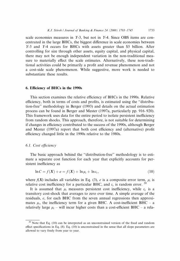
scale economies measures in Y-3, but not in Y-4. Since OBS items are con-centrated in the large BHCs, the biggest di�erence in scale economies betweenY-3 and Y-4 occurs for BHCs with assets greater than $5 billion. Aftercontrolling for size through other assets, equity capital, and physical capital,there may not be enough independent variation in the non-traditional mea-sure to materially e�ect the scale estimates. Alternatively, these non-tradi-tional activities could be primarily a pro®t and revenue phenomenon and nota cost-side scale phenomenon. While suggestive, more work is needed tosubstantiate these results.

6. E�ciency of BHCs in the 1990s

This section examines the relative e�ciency of BHCs in the 1990s. Relativee�ciency, both in terms of costs and pro®ts, is estimated using the ``distribu-tion-free'' methodology in Berger (1993) and details on the actual estimationprocess can be found in Berger and Mester (1997a, particularly pp. 916±920).This framework uses data for the entire period to isolate persistent ine�ciencyfrom random shocks. This approach, therefore, is not suitable for determiningif changes in e�ciency contributed to the success of the 1990s, although Bergerand Mester (1997a) report that both cost e�ciency and (alternative) pro®te�ciency changed little in the 1990s relative to the 1980s.

6.1. Cost e�ciency

The basic approach behind the ``distribution-free'' methodology is to esti-mate a separate cost function for each year that explicitly accounts for per-sistent ine�ciency as

lnC � f �X� � e � f �X� � lnli � lnec; �10�where f(X) includes all variables in Eq. (3), e is a composite error term, li isrelative cost ine�ciency for a particular BHC, and ec is random error. 20

It is assumed that li measures persistent cost ine�ciency, while ec is atransitory cost-shock that averages to zero over time. A simple average of theresiduals, e, for each BHC from the seven annual regressions then approxi-mates li, the ine�ciency term for a given BHC. A cost-ine�cient BHC ± arelatively large li ± will incur higher costs than a cost-e�cient BHC ± a rela-

20 Note that Eq. (10) can be interpreted as an unconstrained version of the ®xed and random

e�ect speci®cations in Eq. (8). Eq. (10) is unconstrained in the sense that all slope parameters are

allowed to vary freely from year to year.


tively small li ± holding constant variation in input prices, output choices, andother explanatory variables. 21

The BHC with the smallest ine�ciency term for 1991±1997, lmin, is labeledthe ``best cost-practice'' BHC since it incurs the lowest costs, conditional on theother variables. Every other BHC can then be compared to the best cost-practice BHC by asking the following counter-factual question ± what costswould a particular BHC incur if it were as e�cient as the best cost-practiceBHC? This measure of relative cost e�ciency is de®ned as

C-EFF � exp �f �X� � exp � lnlmin�exp �f �X� � exp � lnli�

� lmin

li; �11�

where lmin is the smallest observed ine�ciency term from the best cost-practiceBHC.

This measure of e�ciency ranges between 1.0 for the most e�cient BHC andapproaches 0 for a BHC with maximum ine�ciency. C-EFF represents theproportion of costs that are e�ciently employed, e.g., if C-EFF� 0.75 for aparticular BHC, then 25% of its costs are attributed to cost ine�ciency.

6.2. Pro®t e�ciency

One can examine pro®t e�ciency in a similar way by estimating the fol-lowing pro®t function:

ln�P� h� � f �X� � e � f �X� � lnpi � lneP; �12�where h is a constant set equal to one plus the absolute value of the minimumpro®ts each year to avoid taking logs of a negative number as described abovefor Eq. (3). Again, the regression is run separately for each year and the meanresidual for each BHC is interpreted as an estimate of persistent pro®t e�-ciency, pi.

The BHC with the largest pi for 1991±1997 is then labeled the ``best pro®t-practice BHC'' since it earns the most pro®ts, conditional on all other vari-ables. To measure relative pro®t ine�ciency, ask the following counter-factualquestion ± how much pro®t could a particular BHC earn if it were as e�cientas the best pro®t-practice BHC? This measure of relative pro®t e�ciency isde®ned as

P-EFF � exp �f �X � � exp � ln�pi�� ÿ hexp �f �X�� exp � ln�pmax�� ÿ h

; �13�

21 The truncation process of Berger and Mester (1997a) is used to assign less extreme values for

BHCs with very large average residuals, above the 95th percentile or below the 5th percentile, since

it is likely that the random component was not completely removed in these cases.


where pmax is the pro®t e�ciency for the best pro®t-practice BHC. Each ®ttedvalue is evaluated using parameters estimated for each year and the right-handside variables of a given bank in that year. The ®tted values are then averagedfor each BHC to generate a single estimate for each BHC. 22

This measure of pro®t e�ciency ranges from 1 for the most pro®t e�cientbank to )1 for an in®nitely pro®t ine�cient bank. P-EFF represents theproportion of potential pro®ts that are earned, e.g., if P-EFF equals 0.75, thenthe BHC is losing about 25% of potential pro®ts to ine�ciency.

6.3. Estimates of cost and pro®t e�ciency

This procedure yields a single measure of relative cost e�ciency, C-EFF,and relative pro®t e�ciency, P-EFF, for reach of the BHCs in the sample.Again, C-EFF and P-EFF were estimated using each of the four alternativespeci®cations. Since true e�ciency likely varies for a given BHC over time asbusiness conditions and the operating environment change, these e�ciencyterms should be interpreted as the average e�ciency of a given BHC relative tothe best practice BHC for the entire period 1991±1997.

6.3.1. Mean and variation in e�ciencyTable 6 presents weighted averages of C-EFF and P-EFF across all BHCs

for each of the four output speci®cations. In all cases, weights equal the de-nominator of the e�ciency ratios so that the estimates re¯ect the proportion ofresources lost to ine�ciency. Note that C-EFF is the same in the Y-3 and Y-4speci®cation since it is irrelevant if OBS items are treated as an output or a

Table 6

Average cost and pro®t e�ciency, 1991±1997a

Output speci®cation C-EFF P-EFF

Y-1: Business loans, consumer loans, securities 0.909 0.606

(0.049) (0.165)

Y-2: Business loans, consumer loans, securities, net non-interest

income

0.887 0.720

(0.043) (0.101)

Y-3: Business loans, consumer loans, securities, o�-balance sheet

items as an output

0.911 0.659

(0.048) (0.129)

Y-4: Business loans, consumer loans, securities, o�-balance sheet

items as a ®xed netput

0.911 0.634

(0.048) (0.150)

a All e�ciency measures are weighted averages for all 661 BHCs with weights equal to the de-

nominator of the e�ciency ratio. C-EFF� 1 for the ``best cost-practice'' BHC and p-EFF � 1 for

the best pro®t-practice BHC. Standard deviations are in parentheses.

22 Note that this does not reduce to the ratio of ine�ciency terms as in the cost function due to

the h term.


®xed netput in the cost function analysis, but P-EFF varies since the depen-dent variable is di�erent.

The weighted average C-EFF for all 661 BHCs ranges from 0.89 to 0.91,which implies that about 10% of incurred costs in the 1990s can be attributed tocost ine�ciency relative to the best cost-practice BHC. The weighted average ofP-EFF ranges from 0.61 for Y-1, the traditional output speci®cation, to 0.72

Fig. 4. Distribution of cost e�ciency (Y-4), 1991±1997.

Fig. 5. Distribution of Pro®t E�ciency (Y-4), 1991±1997.


for Y-2, which includes net non-interest income as an output. This implies thatine�ciency forces BHCs to forego about one-third of the potential pro®ts thatthe best pro®t-practice BHC could earn. An important conclusion is that thatfailure to account for non-traditional activities understates pro®t e�ciency.

A second notable ®nding is that the distribution of C-EFF is narrow relativeto the distribution of P-EFF, i.e., the standard deviation of C-EFF far exceedsthe standard deviation of P-EFF for all speci®cations. As an example, Figs. 4and 5 plot the distribution of C-EFF and P-EFF from the Y-4 speci®cation.This suggests that BHCs are more comparable in their ability to choose cost-minimizing inputs mixes and there is much more heterogeneity with respect topro®t e�ciency. Although both distributions are roughly bell-shaped, theShapiro±Wilk and Shapiro±Francia tests formally reject the null hypothesis ofa normal distribution for all speci®cations except P-EFF for Y-2. Finally, theskewness coe�cient, de®ned as l3/r3 where l3 is the third and r2 is the secondmoment about the mean, is less than zero for all distributions (except P-EFFfor Y-2), indicating that those distributions are skewed left.

These results are similar to earlier estimates that examined commercialbanks. Berger and Humphrey (1997), for example, report mean cost e�ciencyof 0.84 across 110 studies of US banks. In a comprehensive comparison ofalternative measurement techniques, Bauer et al. (1998) estimate mean e�-ciency of 0.83 across seven parametric models for 683 large banks (assetsgreater $100 million) for 1977±1988. Likewise, Berger and Mester (1997a) re-port average cost e�ciency of 0.87 and (alternative) pro®t e�ciency of 0.46 fora sample of 5946 individual banks. Rogers (1998), which includes net non-interest income as a bank output, reports cost-e�ciency of 0.71 and pro®te�ciency of 0.71 in states with statewide branching. These results suggest thatBHCs as an aggregate entity are much more cost e�cient and slightly morepro®t e�cient than the individual subsidiary banks. 23

One interesting hypothesis concerning these ®ndings concerns the role ofinformation technology. Prasad and Harker (1997) argue that informationtechnology may not provide real bene®ts in retail banking, but rather is a``strategic necessity'' that merely allows a bank to remain competitive. If this isprimarily a cost-side phenomenon, one would expect relatively equal costssince all banks have access to the same fundamental technology. Consistentwith these ®ndings, pro®tability would then vary more and would be largelydependent on the idiosyncratic ability of bank managers. Since ®nancial

23 Nonparametric techniques typically yield far lower e�ciency estimates. Bauer et al. (1998),

however, conclude `ìt seems fairly clear that the parametric approaches are generally more

consistent with what are generally believed to be the competitive conditions in the banking

industry'' (p. 107).


institutions are very intensive users of information technology, more workneeds to be devoted to this issue.

6.3.2. E�ciency correlatesTo examine the reasonability of these estimates, Table 7 presents Spearman

rank-correlations between all e�ciency terms and several other relevant ac-counting variables, e.g., ROA, ROE, C/A, where the three accounting variablesare annual means for 1991±1997. Consistent with previous results in this paper,there is very high correlation between the C-EFF and P-EFF estimates fromthe alternative speci®cations, e.g., between 0.89 and 1.00 on the cost side andbetween 0.87 and 0.99 on the pro®t side. Moreover, these rank correlationssuggest that both C-EFF and P-EFF are indeed measuring the average e�-ciency of the BHCs since both are positively and signi®cantly correlated withROA and ROE, but negatively and signi®cantly correlated with C/A.

It is somewhat surprising that C-EFF and P-EFF are negatively, althoughoften insigni®cantly, correlated and this could re¯ect either mismeasuredproduct quality, o�setting expertise on the cost and revenue sides, or di�erentcompetitive pressures in the input and output markets across BHCs. In anycase, cost e�ciency does not imply pro®t e�ciency.

As a second internal consistency check, these e�ciency estimates werecompared to the estimated ®xed e�ect from simple panel regressions, e.g., Eq.(6) without the time-related parameters. The correlation between the e�ciencyestimate from the distribution-free approach and the ®xed e�ect for eachoutput speci®cation was quite strong ± typically near 0.80 for the cost functionsand between 0.60 and 0.70 for the pro®t functions. 24 The lack of perfectcorrelation simply re¯ects the di�erences in the methodology, e.g., the ®xede�ect model constrains all slopes to be constant for all years, while the dis-tribution-free method allows each slope to vary, and the log-transformationand truncation in the distribution-free approach. Nonetheless, the strongcorrelation provides a useful robustness check for the distribution-freemethod. 25

6.3.3. E�ciency and sizeOne of the primary motivations for consolidation is improved e�ciency, so

an important question is whether large BHCs are more e�cient than smallerones. The results, Figs. 6 and 7 and Table 8, show slight evidence of improvedcost e�ciency and a slight decrease in pro®t e�ciency for large BHCs. In termsof pro®t e�ciency, however, there are large di�erences across the alternative

24 Note that the cost function correlation was negative since a large unobserved component, the

®xed e�ect, implies low cost e�ciency.25 I thank a referee for suggesting this robustness check.


Tab

le7

Ra

nk

-co

rrel

ati

on

of

e�ci

ency

esti

ma

tes

an

da

cco

un

tin

gvari

ab

les,

1991±1997

a

C-E

FF

P-E

FF

RO

AR

OE

C/A

Y-2

Y-3

Y-4

Y-1

Y-2

Y-3

Y-4

C-E

FF

Y-1

0.8

90

.99

0.9

9)

0.0

2)

0.2

0)

0.0

2)

0.0

20.0

90.0

7)

0.3

3

(0.0

0)

(0.0

0)

(0.0

0)

(0.5

8)

(0.0

0)

(0.5

8)

(0.5

4)

(0.0

2)

(0.0

5)

(0.0

0)

Y-2

0.8

90.8

9)

0.1

7)

0.2

0)

0.1

6)

0.1

70.1

10.1

2)

0.2

1

(0.0

0)

(0.0

0)

(0.0

0)

(0.0

0)

(0.0

0)

(0.0

0)

(0.0

0)

(0.0

0)

(0.0

0)

Y-3

1.0

0)

0.0

3)

0.2

0)

0.0

3)

0.0

30.0

90.0

8)

0.3

3

(0.0

0)

(0.4

5)

(0.0

0)

(0.5

3)

(0.4

9)

(0.0

2)

(0.0

5)

(0.0

0)

Y-4

)0.0

3)

0.2

0)

0.0

3)

0.0

30.0

90.0

8)

0.3

3

(0.4

4)

(0.0

0)

(0.5

3)

(0.4

8)

(0.0

2)

(0.0

5)

(0.0

0)

P-E

FF

Y-1

0.8

70.9

80.9

90.2

10.3

3)

0.3

6

(0.0

0)

(0.0

0)

(0.0

0)

(0.0

0)

(0.0

0)

(0.0

0)

Y-2

0.8

70.8

70.2

30.4

1)

0.2

2

(0.0

0)

(0.0

0)

(0.0

0)

(0.0

0)

(0.0

0)

Y-3

0.9

90.2

00.3

3)

0.3

5

(0.0

0)

(0.0

0)

(0.0

0)

(0.0

0)

Y-4

0.2

00.3

3)

0.3

5

(0.0

0)

(0.0

0)

(0.0

0)

RO

A0.6

5)

0.3

3

(0.0

0)

(0.0

0)

RO

E)

0.1

1

(0.0

0)

aS

pea

rman

ran

kco

rrel

ati

on

an

dp-v

alu

esfo

rte

sto

fze

roco

rrel

ati

on

inp

are

nth

eses

.R

OA

,R

OE

,an

dC

/Aare

all

sim

ple

aver

ages

for

each

BH

Cfo

r

19

91±

19

97

.


output speci®cations which suggests that previous research that failed to in-clude non-traditional activities may have signi®cantly understated pro®t e�-ciency for large BHCs and banks.

Fig. 6 plots the weighted average C-EFF for each output speci®cation acrossasset deciles. There is little variation across the four speci®cations and only a

Fig. 7. Pro®t e�ciency by size class, 1991±1997.

Fig. 6. Cost e�ciency by size class, 1994±1997.


Ta

ble

8

Av

era

ge

cost

an

dp

ro®

te�

cien

cy,

19

91±

19

97

a

Siz

eO

bs.

Mea

n

ass

ets

Y-1

Y-2

Y-3

Y-4

C-E

FF

P-E

FF

C-E

FF

P-E

FF

C-E

FF

P-E

FF

C-E

FF

P-E

FF

All

66

13

87

2.7

0.9

09

0.6

06

0.8

87

0.7

20

0.9

11

0.6

59

0.9

11

0.6

34

(0.0

49

)(0

.165)

(0.0

43)

(0.1

01)

(0.0

48)

(0.1

29)

(0.0

48)

(0.1

50)

16

71

64

.80

.90

00.7

37

0.8

59

0.7

34

0.9

00

0.7

37

0.9

00

0.7

32

(0.0

45

)(0

.104)

(0.0

42)

(0.0

94)

(0.0

43)

(0.1

03)

(0.0

43)

(0.1

02)

26

62

16

.40

.90

60.7

37

0.8

62

0.7

26

0.9

04

0.7

33

0.9

04

0.7

29

(0.0

56

)(0

.123)

(0.0

48)

(0.1

08)

(0.0

55)

(0.1

20)

(0.0

55)

(0.1

20)

.

36

62

50

.00

.89

80.7

65

0.8

58

0.7

60

0.8

96

0.7

57

0.8

96

0.7

53

(0.0

41

)(0

.118)

(0.0

41)

(0.1

10)

(0.0

41)

(0.1

14)

(0.0

41)

(0.1

15)

46

62

98

.60

.90

80.7

32

0.8

71

0.7

33

0.9

05

0.7

30

0.9

05

0.7

26

(0.0

41

)(0

.131)

(0.0

38)

(0.1

19)

(0.0

40)

(0.1

30)

(0.0

40)

(0.1

29)

56

63

59

.80

.91

20.7

21

0.8

72

0.7

26

0.9

10

0.7

16

0.9

10

0.7

10

(0.0

44

)(0

.109)

(0.0

38)

(0.0

84)

(0.0

43)

(0.1

06)

(0.0

43)

(0.1

08)

66

64

49

.20

.90

90.7

05

0.8

73

0.7

12

0.9

08

0.6

97

0.9

08

0.6

93

(0.0

52

)(0

.131)

(0.0

43)

(0.1

02)

(0.0

52)

(0.1

26)

(0.0

52)

(0.1

26)

76

66

26

.60

.91

40.7

40

0.8

75

0.7

42

0.9

12

0.7

33

0.9

12

0.7

31

(0.0

40

)(0

.128)

(0.0

40)

(0.0

97)

(0.0

40)

(0.1

28)

(0.0

39)

(0.1

26)

86

61

00

8.9

0.9

09

0.7

22

0.8

77

0.7

38

0.9

07

0.7

24

0.9

07

0.7

18

(0.0

52

)(0

.138)

(0.0

42)

(0.0

98)

(0.0

52)

(0.1

30)

(0.0

52)

(0.1

32)

96

62

58

2.0

0.9

16

0.7

27

0.8

87

0.7

48

0.9

14

0.7

25

0.9

14

0.7

19

(0.0

32

)(0

.118)

(0.0

26)

(0.0

95)

(0.0

32)

(0.1

17)

(0.0

32)

(0.1

18)

10

66

32

,800

.00

.90

80.5

84

0.8

89

0.7

17

0.9

11

0.6

47

0.9

11

0.6

18

(0.0

51

)(0

.163)

(0.0

45)

(0.1

01)

(0.0

49)

(0.1

28)

(0.0

50)

(0.1

50)

aA

lle�

cien

cym

easu

res

are

wei

gh

ted

av

era

ges

wit

hw

eigh

tseq

ual

toth

ed

eno

min

ato

ro

fth

ee�

cien

cyra

tio

.C

-EF

F�

1fo

rth

eb

est

cost

-pra

ctic

eB

HC

an

dP

-EF

F�

1fo

rth

eb

est

pro

®t-

pra

ctic

eB

HC

.S

tan

dard

dev

iati

on

sare

inp

are

nth

eses

.M

ean

ass

ets

are

inm

illi

on

so

f1997

do

llars

.


slight increase in C-EFF with size, particularly for Y-2. In addition, cost e�-ciency from Y-2 is the lowest of the four speci®cations, which might re¯ect theuse of an income variable as an output proxy. The estimates across size classes,however, are not signi®cantly di�erent, so one cannot draw ®rm conclusions.

Fig. 7 plots the weighted average P-EFF for each output speci®cationacross the same asset deciles. The results show larger di�erences across bothsize and output speci®cations, with the most pronounced di�erences for thelargest size group. These BHCs, with average assets of $33 billion, show P-EFF of only 0.58 compared to over 0.70 for other size BHCs, when non-traditional activities are ignored in speci®cation Y-1. The same trend towardlower P-EFF in larger BHCs is evident, though less pronounced, in theother speci®cations. This is reasonable since large BHCs are much moreactive in these types of non-traditional activities and failure to account forthem imposes a systematic bias that understates measured e�ciency forlarge BHCs.

This ®nding of similar C-EFF and lower P-EFF for large BHCs seems tocontradict the scale economy ®ndings and the ROA averages by size group. Itshould be pointed out, however, that the scale economy ®ndings were esti-mated only from a cost function and there is little di�erence in C-EFF acrossdi�erent sizes. The di�erences between C-EFF and P-EFF suggest that largeBHCs incur costs in the same manner as smaller BHCs so cost e�ciency doesnot vary, but they earn revenue from alternative sources, e.g., increased feeincome or revenue from OBS activities. Thus, P-EFF is biased the most whenthese non-traditional activities are excluded.

These results suggest that signi®cant ine�ciencies existed in the US com-mercial banking industry in the 1990s. Despite the strong overall performance,roughly 10% of costs were due to ine�ciency and 30±40% of potential pro®tswere missed. Moreover, e�ciency does not signi®cantly increase with bank sizeas one might expect if economies of scale are an important determinant ofsuccess. Rather, there are e�cient and pro®table BHCs in every size class andincreased size does not guarantee success.

7. Conclusions

This paper examines the factors that contributed to the improved perfor-mance of US BHCs in the 1990s. The empirical results from several alternativeoutput speci®cations suggest that productivity growth and economies of scalewere the driving forces that kept costs per asset low and allowed BHCs toexperience strong performance since 1991. The ®nding of steady productivitygrowth, in particular, is important since it is consistent with the idea that themassive investment in new technology is working to improve the performanceof the banking industry.


Despite these gains, however, these results indicate substantial ine�ciencyduring the 1990s, especially with regard to pro®ts. That is, BHCs seem betterable to minimize costs relative to the most cost e�cient bank holding companythan to maximize pro®ts relative to the most pro®t e�cient bank holdingcompany. Moreover, the ability to be cost e�cient does not necessarily implypro®t e�ciency as output mix choices appear separate from the input choices.This leaves an important role for bank managers as determinants of success.

Taken together, these results suggest continued improvement in the USbanking industry. The current trend toward consolidation and mergers o�ersone way to reduce the overall ine�ciency and unexploited scale economies thatprevented performance from being even stronger in the 1990s. As more assetsare held by BHCs near the optimal size and the most ine�cient BHCs areacquired and merged with more e�cient ®rms, the performance of the overallindustry should improve. As a ®nal caveat, however, larger size does notguarantee success. The evidence shows substantial dispersion in performanceacross asset classes and the most successful BHCs in all size classes showsimilar performance. This suggests that idiosyncratic factors like managementability remain a crucial factor for success in the US banking industry.

Acknowledgements

I would like to thank Michael Boldin, Gail Fosler, Bob McGuckin, TuckerScott, Phil Strahan, seminar participants at the Conference Board and theFederal Reserve Bank of New York, and two anonymous referees for helpfulcomments on an earlier draft. Ichiro Tange provided excellent research as-sistance. This paper re¯ects the views of the author only and does not nec-essarily re¯ect the views of the Federal Reserve Bank of New York, the FederalReserve System, or their sta�s.

References

Akhavein J.D., Berger, A.N., Humphrey, D.B., 1997. The e�ects of megamergers on e�ciency and

prices: Evidence from a bank pro®t function. Finance and Economic Discussion Series 1997-9.

Federal Reserve Board, Washington, DC.

Bauer, P., Berger, A., Ferrier, G.D., Humphrey, D.B., 1998. Consistency conditions for regulatory

analysis of ®nancial institutions: A comparison of frontier e�ciency methods. Journal of

Economics and Business 50, 85±114.

Berger, A.N., 1993. Distribution-free estimates of e�ciency in the US banking industry and tests of

the standard distributional assumptions. Journal of Productivity Analysis 4, 261±292.

Berger, A.N., Kashyap, A.K., Scalise, J.M., 1995. The transformation of the US banking industry:

What a long, strange trip it is been. Brookings Papers on Economic Activity 2, 55±218.


Berger, A.N., Hancock, D., Humphrey, D.B., 1993. Bank e�ciency derived from the pro®t

function. Journal of Banking and Finance 17, 317±347.

Berger, A.N., Humphrey, D.B., 1992. Measurement and e�ciency issues in commercial banks. In:

Griliches, Z. (Ed.), Measurement Issues in the Service Sectors. University of Chicago Press,

Chicago, IL. pp. 245±279.

Berger, A.N., Humphrey, D.B., 1997. E�ciency of Financial Institutions: International Survey and

Directions for Future Research. Finance and Economic Discussion Series 1997-11. Federal

Reserve Board, Washington, DC.

Berger, A.N., Mester, L.J., 1997a. Inside the black box: What explains di�erences in the e�ciencies

of ®nancial institutions. Journal of Banking and Finance 21, 895±947.

Berger, A.N., Mester, L.J., 1997b. E�ciency and productivity trends in the US commercial banking

industry: A comparison of the 1980s to the 1990s. Paper presented at the CSLS Conference on

Service Centre Productivity and the Productivity Paradox.

Berger, A.N., Hanweck, G.A., Humphrey, D.B., 1987. Competitive viability in banking: Scale,

scope and product mix economies. Journal of Monetary Economics 20, 501±520.

Chamberlain, G., 1984. Panel data. In: Griliches, Z., Intriligator, M.D. (Eds.), Handbook of

Econometrics, vol. II. Elsevier, Amsterdam.

English, W.B., Nelson, W.R., 1998. Pro®ts and balance sheet developments at US commercial

banks in 1997. Federal Reserve Bulletin 391±419.

Federal Deposit Insurance Corporation, 1998a. The FDIC Quarterly Banking Pro®le. Fourth

Quarter, 1997.

Federal Deposit Insurance Corporation. 1998b. The FDIC Quarterly Banking Pro®le. Second

Quarter, 1998.

Federal Deposit Insurance Corporation. 1997. History of the Eighties±Lessons for the Future: An

Examination of the Banking Crisis of the 1980s and Early 1990s. Federal Deposit Insurance

Corporation. Washington, DC.

Grabowski, R., Rangan, N., Rezvanian, R., 1993. Organizational forms in banking: An empirical

investigation of cost e�ciency. Journal of Banking and Finance 17, 531±538.

Holland, D., Inscoe, D., Waldrop, R., Kuta, W., 1996. Interstate banking: The past, present, and

future. FDIC Banking Review, Fall.

Hughes, J.P., Mester, L.J., 1998. Bank capitalization and cost: Evidence of scale economies in risk

management and signaling. The Review of Economics and Statistics, 314±325.

Hughes, J.P., Landg, W., Mester, L.J., Moon, C.-G., 1996. E�cient banking under interstate

branching. Journal of Money, Credit and Banking 28 (4), 1045±1071.

Humphrey, D.B., Pulley, L.B., 1997. BankÕs responses to deregulation: Pro®ts, technology, and

e�ciency. Journal of Money Credit and Banking 29 (1), 73±93.

Jagtiani, J., Khanthavit, A., 1996. Scale and scope economies at large banks: Including o�-balance

sheet products and regulatory e�ects (1984±1991). Journal of Banking and Finance 20, 1271±

1287.

Jagtiani, J., Nathan, A., Sick, G., 1995. Scale econmies and cost complementarities in

commercial banks: On- and o�-balance sheet activities. Journal of Banking and Finance

19, 1175±1189.

Lang, G., Welzel, P., 1996. E�ciency and technical progress in banking: Empirical results for a

panel of German cooperative banks. Journal of Banking and Finance 20, 1003±1023.

Newman, J., Shrieves, R., 1993. Multibank holding company e�ect on cost e�ciency in banking.

Journal of Banking and Finance 17, 709±732.

Prasad, B., Harker, P.T., 1997. Examining the contribution of information technology toward

productivity and pro®tability in US. Retail Banking. Wharton Financial Institutions Center,

Philadelphia, PA, 97±99.

Riveard, R.J., Thomas, C.R., 1997. The e�ect of interstate banking on large bank holding company

pro®tability and risk. Journal of Economics and Business 49, 61±76.


Rogers, K.E., 1998. Nontraditional activities and the e�ciency of US commercial banks. Journal of

Banking and Finance 22, 467±482.

Roland, K.P., 1997. Pro®t persistence in large US bank holding companies: An empirical

investigation. Economic Working Paper 97-2. Comptroller of the Currency, Washington, DC.

January.

Sealey, C., Lindley, J., 1977. Inputs, outputs, and a theory of production and cost at depository

®nancial institutions. Journal of Finance 32, 1251±1266.

Spong, K., 1994. Bank Regulation: Its Purposes, Implementation, and E�ects. Federal Reserve

Bank of Kansas City, Kansas City, MO.


Documents

How did bank holding companies prosper in the 1990s?directory.umm.ac.id/Data Elmu/jurnal/J-a/Journal Of Banking And Finance...How did bank holding companies prosper in the 1990s? Kevin