Embed Size (px)
Citation preview

i
HOUSEHOLD TRAVEL/ACTIVITY DECISIONS
by
CATHERINE THERESA LAWSON
A dissertation submitted in partial fulfillment of therequirements for the degree of
DOCTOR OF PHILOSOPHYin
URBAN STUDIES
Portland State University1998

ii
ACKNOWLEDGMENTS
I would like to express my deep appreciation to my advisor and committee
Chair, Dr. James G. Strathman, for his valuable advice and encouragement
throughout my doctoral program and dissertation process. Sincere appreciation and
gratitude are also extended to the rest of my committee, Drs. Kenneth J. Dueker,
Anthony M. Rufolo, Abdul Qayum, and Thomas P. Potiowsky. In addition, I would
like to thank Peter Gordon from the University of Southern California, Frank
Koppelman from Northwestern University, and Ryuichi Kitamura from University of
California at Davis, for their encouragement. I am especially grateful to the late Eric
I. Pas, for his interest and guidance.
I would like to thank Brian Chase, Director of Facilities at Portland State
University, and all his staff, for their encouragement and kindness. Some of my
research would not have been possible without the help of David B. Gardner and
Chuck C. Cooper. I would also like to thank my colleagues, Drs. John Bowman,
Zhong-Ren Peng, and Matthew Karlaftis, for being such good role models. I am
very grateful to the many individuals who listened to my ideas, directed my studies,
and made my lattes.
Finally, I am greatly indebted to my parents, my brothers, my children
(Anathea, Cassea, and Benjamin), and my grandchild (Johannah), for their love over
so many years of learning.

iii
TABLE OF CONTENTS
PAGE
Acknowledgments ......................................................................... i
List of Tables...............................................................................vii
List of Figures ..............................................................................xi
Chapter 1: INTRODUCTION ................................................ 1
1.1 General Background.............................................. 1
1.2 Research Objective ............................................... 3
1.3 Empirical Analysis ................................................ 4
1.3.1 Data........................................................... 4
1.3.2 Utility Maximization Models ...................... 5
1.3.3 Applications............................................... 5
1.4 Overview of the Dissertation ................................. 6
Chapter 2: GENERAL BACKGROUND................................ 7
2.1 Introduction .......................................................... 7
2.2 Early History of Travel Forecasting ....................... 8
2.3 First Generation Travel Demand Models...............10
2.4 “Demand” for Travel Demand Models..................17
2.5 Second Generation Models...................................21
2.6 Model Improvements............................................25
2.6.1 Changes in Scope and Size........................25
2.6.2 Income and Time Constraints....................26
2.6.3 Multiple Stops and Travel Patterns............38
2.7 State of the Art Models ........................................44
2.8 Summary..............................................................49

iv
Chapter 3: DECISION TO TRAVEL ....................................51
3.1 Introduction .........................................................51
3.2 Economic Perspective...........................................52
3.3 Derived Demand for Transport .............................54
3.4 Consumer Demand ...............................................55
3.5 “New Home Economics”......................................57
3.6 Household Production Approach..........................61
3.6.1 Monetary Influences..................................63
3.6.2 Temporal Influences..................................68
3.6.3 Socio-demographic Influences...................71
3.6.3.1 Gender........................................71
3.6.3.2 Age.............................................72
3.6.3.3 Household Structure ...................73
3.6.3.4 Years in the Home ......................81
3.6.3.5 Employment Status .....................81
3.6.3.6 Total Household Income.............83
3.6.3.7 Vehicles per Household...............84
3.6.4 Activity Location Decisions ......................85
3.7 Summary..............................................................87
Chapter 4: HOUSEHOLD TRAVEL/ACTIVITYDECISIONS: A CONCEPTUAL MODEL..........89
4.1 Introduction .........................................................89
4.2 Conceptual Model ................................................90
4.3 Summary............................................................101

v
Chapter 5: EMPIRICAL ANALYSIS ..................................102
5.1 Introduction .......................................................102
5.2 Data Collection and Classification.......................102
5.3 Chi Square Analysis............................................106
5.3.1 Hypothesis One ........................................106
5.3.1.1 Place of Work .............................106
5.3.1.2 Place of Meals.............................106
5.3.1.3 Place of Household Business .......107
5.3.1.4 Place of Household Maintenance .107
5.3.1.5 Place of Household Obligations ...107
5.3.1.6 Place of Exercise.........................107
5.3.1.7 Place of Rest & Relaxation..........107
5.3.1.8 Place of Amusements ..................108
5.3.2 Hypothesis Two........................................108
5.3.2.1 Place of Work .............................108
5.3.2.2 Place of Meals.............................108
5.3.2.3 Place of Household Business .......109
5.3.2.4 Place of Household Maintenance .109
5.3.2.5 Place of Household Obligations ...109
5.3.2.6 Place of Exercise.........................109
5.3.2.7 Place of Rest & Relaxation..........109
5.3.2.8 Place of Amusements ..................110
5.4 Summary............................................................112
Chapter 6: RANDOM UTILITY MODELS.........................113
6.1 Introduction .......................................................113
6.2 Random Utility Models.......................................113
6.3 Logit Model .......................................................115
vi
6.3.1 Specification ...........................................115
6.3.2 Peak Period Models ................................124
6.3.3 Socio-demographic Models.....................142
6.4 Summary............................................................147
Chapter 7: APPLICATIONS ...............................................150
7.1 Introduction .......................................................150
7.2 Odds Ratios........................................................150
7.3 Representative Cases ..........................................153
7.4 Discussion ..........................................................164
7.4.1 Socio-demographic Impacts ....................166
7.4.1.1 Gender ........................................166
7.4.1.2 Age .............................................167
7.4.1.3 Household Structure....................168
7.4.1.4 Years in the Home.......................169
7.4.1.5 Employment Status .....................169
7.4.1.6 Total Household Income .............170
7.4.2 Time of Day............................................171
7.4.3 Activity Types and Classification.............173
7.5 Summary............................................................173
Chapter 8: DISCUSSION AND CONCLUSIONS...............175
8.1 Introduction .......................................................175
8.2 Conclusions........................................................175
8.3 Further Applications ...........................................178
8.4 Direction of Future Research ..............................180
8.4.1 Use of Geographic Information Systems 180
8.4.2 Additional Socio-demographic Variables.182
8.4.2.1 Gender ........................................182

vii
8.4.2.2 Household Structure....................183
8.4.2.3 Years in the Home.......................183
8.4.2.4 Employment Status .....................184
8.4.3 Time of Day............................................184
8.4.4 Activity Types and Classifications ...........185
8.5 Contribution to Research....................................185
REFERENCES .........................................................................189

viii
LIST OF TABLES
TABLE TITLE PAGE
5.1 Classification Schemes for Activity Data ........................104
5.2 Classification of Activities that Occur Both in andOut of the Home............................................................105
5.3 Summary of Statistically Significant Effects (p< .05) ......111
6.1 Socio-demographic Variables.........................................115
6.2 Probability of Conducting an Activity Out of the Homefor All Substitutable Activities and Major Groupings......117
6.3 Probability of Conducting an Activity Out of the Homefor All Substitutable Activities, Work, Non-work, HomeProduction and Leisure Activities Over an Entire Day(coefficients) ..................................................................118
6.4 Submodel Equivalence Tests for All SubstitutableActivities........................................................................119
6.5 Probability of Conducting an Individual SubstitutableActivity Out of the Home...............................................120
6.6 Probability of Conducting an Individual SubstitutableHome Production Activity Out of the Home(coefficients) ..................................................................121
6.7 Submodel Equivalence Tests for IndividualSubstitutable Activities...................................................122
6.8 Probability of Conducting an Individual SubstitutableLeisure Activity Out of the Home (coefficients)..............123

ix
6.9 Submodel Equivalence Tests for All SubstitutableActivities........................................................................124
6.10 Number of Substitutable Activities Conducted in theMorning Peak, Evening Peak, and Off-peak Periods.......125
6.11 Probability of Conducting a Substitutable Activity Outof the Home in the AM Peak..........................................126
6.12 Probability of Conducting a Substitutable Activity Outof the Home in the AM Peak (coefficients).....................127
6.13 Submodel Equivalence Tests for SubstitutableActivities (AM)..............................................................128
6.14 Probability of Conducting a Substitutable Activity Outof the Home in the PM Peak .........................................129
6.15 Probability of Conducting a Substitutable Activity Outof the Home in the PM Peak (coefficients) .....................130
6.16 Submodel Equivalence Tests for SubstitutableActivities (PM) ..............................................................131
6.17 Probability of Conducting an Activity Out of theHome for All Substitutable Activities Over FourTime Periods..................................................................132
6.18 Probability of Conducting a Substitutable WorkActivity Out of the Home for Over Four TimePeriods ..........................................................................133
6.19 Probability of Conducting Substitutable Non-workActivity Out of the Home over Four Time Periods ........134
6.20 Probability of Conducting Substitutable HomeProduction Activity Out of the Home over Four TimePeriods...........................................................................135
x
6.21 Probability of Conducting Substitutable LeisureActivity Out of the Home over Four TimePeriods...........................................................................137
6.22 Time Variables...............................................................138
6.23 Probability of Conducting a Substitutable Activity Outof the Home...................................................................139
6.24 Probability of Conducting a Substitutable Activity Outof the Home (AM and PM Peaks) ..................................140
6.25 Tests for the Contribution of New Variables andSubmodel Equivalence Tests ..........................................141
6.26 Socio-demographic Variables.........................................142
6.27 Probability of Conducting a Substitutable Activity Outof the Home (Employment Status and Income Levels)....145
6.28 Probability of Conducting a Substitutable Activity Outof the Home (Household Size) ......................................146
7.1 Odds Ratios of Conducting a Substitutable ActivityOut of the Home............................................................151
7.2 Odds Ratios of Conducting a Substitutable ActivityOut of the Home(Employment Status and Household Size) ......................152
7.3 Probability of Conducting a Substitutable Activity Outof the Home by Employment Status, Household Sizeand Income Group .........................................................154
7.4 Probability of Conducting a Substitutable HomeProduction Activities Out of the Home by Gender andHousehold Size ..............................................................156

xi
7.5 Probability of Conducting a Substitutable HomeProduction Activities Out of the Home by Genderand Age .........................................................................160
7.6 Probability of Conducting a Substitutable Activity Outof the Home by Activity Type and Household Size.........161
7.7 Probability of Conducting a Substitutable Activity Outof the Home by Activity Type and Age...........................162
7.8 Probability of Conducting a Substitutable HomeProduction Activity Out of the Home by Number ofVehicles and Gender ......................................................164
8.1 Additional Socio-demographic Variables........................182
xii
LIST OF FIGURES
FIGURE TITLE PAGE
3.1 Traditional Microeconomic Approach ..............................56
3.2 “New Home Economics” Approach .................................57
3.3 Household Production Approach .....................................63
7.1 Probability of Conducting a Substitutable ActivityOut of the Home by Employment Status, HouseholdSize, and Income Group.................................................155
7.2 Probability of Conducting a Substitutable HomeProduction Activity Out of the Home by Household Sizeand Gender ....................................................................157
7.3 Probability of Conducting a Home Production ActivityOut of the Home by Time of Day and Gender ................159
7.4 Probability of Conducting a Substitutable Activity Outof the Home by Activity Type and Age...........................163

1
CHAPTER ONE
INTRODUCTION
1.1 GENERAL BACKGROUND
Activity-based approaches are expected to provide a better framework for
travel demand modeling because they recognize the interdependence of travel
decisions made by household members and the allocation of household resources,
assignment of tasks, and joint activity engagement. Previous activity-based
approaches have not explicitly incorporated the economic concept of substitution
with respect to activities that can be conducted at home or out of the home. It is
hypothesized that an individual chooses a set of daily activities in order to optimize
his/her overall utility function. Given income, distance, time, and participation
constraints, individuals choose the location for conducting these activities. This
decision can be characterized by a random utility model, such as a binary logit (in or
out of the home).
Activity-based household surveys contain information on what each member
in a household did (activity choice), where (location choice), for how long (activity
duration), and with whom (activity participation). This dissertation uses the Oregon
and Southwest Washington 1994 Activity and Travel Behavior Survey activity data

2
set to examine various factors that influence the location choice of individuals for
activities that can be conducted either in or out of the home.
The demand for travel is considered a derived demand based on the need or
desire to do something in a place other than where you are. The evolution of travel
demand models began with aggregate demand (first-generation) transportation
models, based on observed relations for groups of travelers or on "average"
relations at a zonal level (Ortuzar and Willumsen 1994).
There was a gradual transition from an aggregate to a disaggregate modeling
approach. The disaggregate models (second generation) used individuals or
households, rather than the zones used in the aggregate approach, as the unit of
analysis. The disaggregate approach examined the movements of individuals as they
participated in different activities over a day or longer periods. The data was
collected in the form of travel diaries that reported timing, duration, sequencing and
purposes of trips. This method allowed for analysis of movement patterns within
zones, in addition to between the zones used in aggregate models. During this
transition period, the practice of determining trip generation by zones was replaced
by trip rates for different household types. Gravity models based on zonal
attractiveness were replaced by destination-choice logit models.
Sociodemographic variables are used in transportation demand models on
the assumption that the propensity to travel and trip characteristics vary with the
characteristics of the traveler. The some of the variables assumed to affect travel

3
include income, gender, employment status, age, occupation, household size, and
auto availability. These variables are surrogates for more complex factors such as
gender roles or social status, which are thought to affect the need for activities and
locations that drive the demand for travel.
More recently, activity-based survey data have replaced the traditional
origin-destination (O-D) surveys. Geocoded point data are being used in lieu of
zonal centroids. Microsimulation models are replacing zone-to-zone traffic
assignment models. However, even with these advances in travel forecasting
models, there is a great deal of turmoil in the transportation planning community.
The models that were developed to ensure adequate expansion of the transportation
network are not adequate to address critical concerns for current policy. Models
used for travel forecasting can not be used to determine the consequences of policy
choices which require a level of responsiveness to “demand-side” solutions.
Although a number of extensions have been developed, there is no clear
understanding regarding the nature of the derived demand for travel.
1.2 RESEARCH OBJECTIVE
This dissertation reports an analysis of the decision to undertake an activity
in the home or out of the home and the factors that contribute to that decision.
Conceptually, the analysis is based on a utility maximization process described as
“new home economics”. The understanding of the derived demand for travel, within

4
the context of utility maximization and a household production function, is the
primary focus.
The use of simulation models for transportation planning, such as
TRansportation ANalysis SIMulation System (TRANSIMS), provide a new
opportunity to revisit the incorporation of a more direct approach to the
implementation of economic principles. Without a framework for understanding the
basic level of behavior underlying the use of transport (conducting an activity in or
out of the home) within the context of a household, policies that rely on changes in
behavior can have unanticipated impacts. Equity issues require a new approach to
disaggregating segments of the population with respect to their use of transportation
facilities.
1.3 EMPIRICAL ANALYSIS
1.3.1 Data
Empirically, the analysis uses two-day travel-activity data, collected from
4,451 households in the Portland, Oregon, metropolitan area. After sorting the
activity types into those that can be conducted either in or out of home, a set of chi
square tests are run. Factors examined for their influence on activity location
include the activity itself, gender, and household size.

5
1.3.2 Utility Maximization Models
Given an underlying utility maximizing framework, the discrete choice of
whether to conduct an activity in or out of the home can be characterized using
random utility theory (RUT). To better understand the influences on household
travel/activities decisions, a set of logit models are specified. It should be noted that
this approach assumes that activity participation has been determined prior to the
decision to conduct the activity in or out of the home. Such as assumption
precludes recognition of the possible endogenous nature of activity participation.
The logit regressions provide indications of the influence of activity types in
the aggregate (work, non-work), subgroups of non-work activities (home
production and leisure), and individual activity types, gender, age, household size,
tenure in a home, employment status, income group, number of vehicles and time of
day, on the decision to conduct a “substitutable” activity out of the home. The
results of this analysis are intended to facilitate the development of more complex
models that include activity choice.
1.3.3 Applications
Applications are developed from the logit model coefficients. The odds
ratios are calculated for a set of dummy variables. Representative cases analysis is
used to focus on the probability that a substitutable activity will be conducted out of
the home. Through this process, it is possible to look at the effect of a combination
of factors on a household travel/activity decision to conduct an activity out of the

6
home. The representative cases applications also offer an opportunity to address
equity issues for various populations affected by policy.
1.4 OVERVIEW OF DISSERTATION
Chapter Two describes the general background of the development of travel
forecasting models. Chapter Three uses microeconomic concepts to develop an
understanding of the underlying factors that explain the derived demand for travel.
“New home economics” is used as a framework for understanding of household
travel/activity decisions. Various factors that influence travel/activity behavior are
examined. Chapter Four develops a utility maximizing equations that include
income, distance, time, and participation constraints, for household members.
The empirical aspects of this study begin in Chapter Five with a chi square
analysis. The Oregon and Southwest Washington 1994 Activity and Travel
Behavior Survey data is used for a general understanding of the influences of
sociodemographic variables on the location (in or out of the home) of an activity.
Chapter Six develops a set of logit regressions to determine the influence of various
factors on travel/activity decisions. Chapter Seven uses the logit coefficients to
determine the probability of an individual conducting a substitutable activity out of
the home through a set of representative cases applications, followed by a discussion
of the findings. Chapter Eight concludes with suggestions for future applications
and research.

7
CHAPTER TWO
GENERAL BACKGROUND
2.1 INTRODUCTION
The evolution of travel demand forecasting models has resulted in a set of
models that can not meet the demands being made by policy makers. This section
looks at the history of travel forecasting models and some of the reasons why
problems have arisen with the underlying assumptions and methods of analysis.
During the development of the transportation infrastructure system, certain
requirements for obtaining funding were responsible for establishing relationships
among the providers of the transportation facilities (local and state governments),
the funding agencies (state and federal governments), and the users (local citizens,
businesses and pass-through travelers). Expectations regarding the output of travel
forecasting models have changed, putting pressure on the transportation industry to
make improvements.

8
2.2 EARLY HISTORY OF TRAVEL FORECASTING
The federal government has played a major role in the development of
transportation facilities in the United States. However, prior to 1916, the federal
government had very little control over the development of the transportation
network as rural road construction was typically the responsibility of a county
government. The county road philosophy emphasized the construction of roads on
alignments determined by property lines and section lines. This practice produced
circuitous routing that followed fence lines and ownership patterns. It was accepted
practice that the rights of property owners came first in agricultural districts.
Decisions about transportation improvements reflected the needs of the local
farmers as property owners, using roads to serve farm to market trips.
According to Gifford (1984), there were two predominant strategies for
providing transportation facilities. Road funds could be spread over all the mileage
within a county to increase political visibility or monies could be used on specific
routes to please certain constitutencies. In general, these roads connected the urban
cores within the county, in addition to benefiting certain politically-favored
individuals.
In 1916, the federal government tried to encourage a more equitable, state-
wide perspective with the passage of the 1916 Act. According to the Act, when
funds became available from the federal government to state governments,
restrictions were placed on the provision of roads to insure a more uniform network

9
across states (Pas 1986). These early requirements established a set of relationships
among the providers of the transportation facilities (local and state governments),
the funding agencies (state and federal governments), and the users (local citizens,
businesses and pass-through travelers).
In the 1930s, engineers designed roads that were quickly made obsolete by
the onset of faster and faster vehicles. This embarrassed the engineering industry
and set in motion an agenda for "overprovision" and limited access, under the guise
of "scientific" road building. The stated objective of the designs was to reduce
travel time, using “engineered” solutions. At the same time, standards were
developed in order to facilitate cost estimates for the construction phase. These
standards were applied regardless of the actual demand for travel, the location, or
the environmental circumstances of the road network.
In 1944, the Bureau of Public Roads performed the first origin-destination
(O-D) survey. The survey was an attempt to collect data that would contribute to
an understanding of observed traffic volumes. Prior to this approach, traffic count
studies made no effort to understand the underlying process that was generating the
observed traffic. The motivation for the development of this survey was the
Federal-Aid Highway Act of 1944. This act authorized the expenditure of funds on
urban extensions through federal aid to primary and secondary highway systems.
The results of the early O-D studies were used to describe existing travel patterns as
“desire lines”, indicating schematically the major spatial distribution of trips. A

10
simple extrapolation technique was used to forecast future volumes, based on past
traffic growth rates (Weiner 1997).
2.3 FIRST GENERATION TRAVEL DEMAND MODELS
Beginning in the 1950s, the need for aggressive urban transportation
planning was fueled by rapid population growth in urban areas, rapid growth of
vehicle ownership, and increasing movement of population to suburban locations
(Pas 1986). Attention had been diverted to the war efforts, leading to a lack of
highway construction and increasing reliance on transit. The increased use of
transit, however, occurred without sufficient funding to maintain the deteriorating
capital equipment.
Weiner (1997) points out that a study conducted by Mitchell and Rapkin, in
1954, recognized specific differences in travel behaviors across household types,
(i.e. single individuals, young married couples, families with young children, and
households with elderly). There was an assumption that the social sciences would
provide transportation planners with the necessary understanding of travel
behaviors. Unfortunately, it appears that the interdisciplinary linkages were not
strong enough to encourage sufficient work in this area.
The passage of the Federal-Aid Highway Act of 1962 required urban areas
to use a comprehensive transportation planning process in order to qualify for
federal matching funds for the construction of transportation improvements. This

11
legislation was the first to mandate planning, asserting that there was a federal
concern that urban transportation be integrated with land development.
The Bureau of Public Roads began publishing manuals dealing with technical
areas, leading to procedures that were codified and institutionalized. For example,
the Policy and Procedure Memorandum 50-9, spelled out an interpretation of the
“3C” planning process. This process was to be “continuing, comprehensive, and
cooperative” (Weiner 1997). Pas (1986) points out that this facilitated the
dissemination of forecasting tools to a large audience in a short period of time. At
the same time, it set up an approach that became resistant to change. The
underlying purpose of the models was to justify expansion of the transportation
network. Using this "supply-side" orientation, as long as the growing demand for
travel was accommodated with an “overprovision” of additional facilities, there was
little need to understand the exact nature of the travel needs of households or to
conduct a bona fide demand-side analysis.
The invention of computers helped accelerate a standardized solution to
transportation planning by allowing planners to gather data on a large scale and
develop models that followed a standardized approach. The studies were conducted
at a regional level and required a full-time staff to operate the computer programs.
The Chicago Area Transportation Study (CATS ) is an example of a region-wide
study that incorporated computer technologies.

12
The overall modeling framework, the Urban Transportation Modeling
System (UTMS), was thought to be the best tool for long range planning for its
time. The objective of UTMS was to forecast trip-making patterns, produce a
region-wide transportation plan, and to ultimately justify the development of
highway systems to facilitate travel in urban areas. Again, the purpose of the UTMS
was to ensure an ample supply of transportation facilities, rather than to understand
the actual demand characteristics of travel behaviors.
Typical data assembled for these models included an inventory of the
existing transportation system, such as physical attributes (number of lanes and
grades), volumes and speeds, an inventory of present land uses, journey to work
census data, the socio-economic variables from the census files, and other related
factors. Additional travel data was gathered from a sample of residents in the study
area using household travel surveys. Nearly thirty percent of the transportation
budget was used to deal with the data for these models (Pas 1986).
Early studies used simple random samples of up to twenty percent of the
households in an area. Later studies used much smaller samples and alternative
sampling procedures. Lerman and Manski (1979) looked at sample size design in an
attempt to reduce the cost of data collection for the Urban Mass Transportation
Administrations Service and Methods Demonstration Program. They recognized
that the application of sample design theory to travel demand forecasting was an
“art”. In theory, a balance was to be found between choosing a specification for a

13
model that accurately represented an actual population, while at the same time being
simple enough to provide a useable forecasting tool for transportation planners.
Clearly, the end result of the decision to use zonal data lead to the reliance on a
“stylized” interpretation of the population, based on samples of households within a
zone. The use of zonal “averages” assumes a homogeneity across households, both
in make-up and behavior.
Since federal funding was to be justified by demonstrating growth in trips
rather than on the overall use of travel within a household, the primary focus was on
the trip. Trip purposes were classified by origin and destination, such as work trips,
shopping trips, recreation trips, school trips, business trips, and home trips (Barber
1986). These categories were used to predict travel behavior at the aggregate level
and were reduced to three classifications: home-based work trips, home-based other
trips and non/home-based trips.
The modeling process developed at this time is often referred to as the four-
step or four-stage process. The Urban Transportation Planning System (UTPS)
began with the determination of trip generation rates for each zone. This procedure
used an ordinary least squares (OLS) approach, with trip origins as the dependent
variable and various household characteristics as independent variables. A linear
relationship between trips generated and the independent variables was assumed.
The use of this specification implies that the classical assumptions of linear
regression are not violated. These assumptions include the independence of the

14
independent variables from each other and the error term; error terms that have an
expected mean value of zero; and error terms that are not correlated with
themselves. Clearly, these assumptions could be violated due to the nature of the
independent variables. There may also be heteroskedasticity in the cross-sectional
data and/or a possibility of spatial autocorrelation. The output of this step was the
number of trips generated from each zone.
The second step, the trip distribution model, was based on the notion of a
gravity model. Relying on the concept of "attractiveness" of a zone, trips are
distributed across zones, based on how attractive one zone is in relation to all other
zones. Attractiveness encompasses employment and other descriptors of the
destinations. Gravity models are not based on microeconomic foundations, but
rather on a weighting principle. The resulting distributions might be an artifact of
the modeling process rather than a representation of trade-offs across destinations.
The third stage contains the mode split process. In this modeling process,
the number of trips and destinations are given. At this step in the model, it is only a
matter of determining which mode the population will use, based on a discrete
choice model, such as the multinomial logit. Mode choice is an example of a limited
dependent variable, with each mode assigned a code (i.e. auto, bus, carpool, walk).
The multinomial logit requires an assumption of independence of irrelevant
alternatives (the IIA property) of the choice alternatives. The standard example is

15
the red bus/blue bus problem that allocates the probability of taking a bus
incorrectly, as the color of the bus should not make it a separate choice.
Another problem with this procedure is the effect of the omission of
variables in the utility equation. An alternative-specific constant is used to capture
the average unspecified variables. However, it is also possible that this information
in being captured in the residual (error term) of the model and is correlated with
other variables. An omitted variable may be a very powerful part of the choice
made by the household as to the mode they intend to utilize. Recent research
indicates that the ability to perform interim trips (trip chaining) is more influential in
mode choice than travel time or out of pocket costs (Rosenbloom and Burns 1994).
The final step is the assignment of trips within the transportation network.
According to Ortuzar and Willumsen (1994), the basic premise in assignment is the
assumption of a rational traveller. Although a number of factors are thought to
influence the choice of a particular route, it has not been practical to attempt to
model all these factors. For example, the journey time, distance, fuel costs, scenery,
and habits, all have some effect on which route a driver will choose. The most
common approximation to represent a generalized cost expression for these
elements contains only two factors, time and money costs (proportional to travel
distance). The computer programmers develop a routine that, in most cases, looks
for the shortest route from the origin to the destination (minimal path program). A

16
number of traffic assignment programs allow weights to be applied to travel time
and distance. The program is run iteratively until an “acceptable” solution is found.
The first problem with a sequential process, such as the four-step approach,
is the accumulation of errors throughout the system. Errors made in the first step
continue and grow, producing inaccuracies with each successive step. When the
model is applied to specific zones, it must be assumed that there is strict
homogeneity in the makeup of the households and their behaviors. Once the
parameters are established throughout the entire set of models, there is the
assumption that the coefficients are constant.
Meyer and Miller (1984) point out the many shortcomings of this process as
a "scientific approach to transportation" stemming from it not being grounded in
reality. The authors indicate that although microeconomic foundations are the
conceptual basis for many aspects of transportation, these foundations were not
operationalized into the models, such as UTMS. Instead of conventional demand
functions, transportation modelers/planners used a "vectors of service variables".
Kitamura (1996) notes that the metropolitan studies used aggregate data for
manageability and computability. However, the seriousness of the lack a behavioral
basis is a shortcoming that can not be overlooked. He points to the example of the
impact of a new highway segment, where the model would under-estimate trip
distribution, while mode shift could be over-estimated due to the insensitivity of trip
generation/attraction models to accessibility.

17
The introduction of the computer and its limitations, assumptions of
adequacy of zonal averages and the need to demonstrate continued growth in trips
in order to qualify for federal funds, drove the development and acceptance of the
four-step modeling process. Unfortunately, the “torturing” of the original data
removed the majority of underlying behavioral information regarding the use of
travel for everyday household activities.
2.4 “DEMAND” FOR TRAVEL DEMAND MODELS
By the end of the 1960s, major social upheavals over civil rights and
environmental concerns impacted urban transportation with new issues that had to
be taken into consideration, in addition to engineering and technical efficiency
issues. The transportation industry had maintained its objective of minimizing travel
times, while urban dwellers took the brunt of "scientifically" designed freeway
systems through their neighborhoods and natural resources. For example, the
National Historic Preservation Act of 1966 was based on the recognition that
federal projects had destroyed or damaged thousands of historic properties. In
addition, attention was placed on issues of air and water pollution; dislocation of
homes and businesses; preservation of parkland; and wildlife refuges (Weiner 1997).
Public awareness of the negative impacts of previous transportation planning
brought about by the environmental movement and the involvement of a larger
population (citizen participation), resulted in the end of road-building (supply-side)

18
as the explicitly preferred solution to urban congestion. Citizens were demanding to
be “invited” to all phases of the planning process, from the goal setting through the
analysis of alternatives. Planning agencies were required to seek out public input.
The National Environmental Policy Act of 1969 (NEPA) established the
Council on Environmental Quality and required all legislation and major federal
actions to include a provision for environmental impact statements (EIS). Important
elements of this legislation include the explicit requirement of gathering information
on uhe environmental impacts of proposed actions, unavoidable impacts, alternatives
to the actions, the relationship between short- and long-term impacts, and
irretrievable commitments of resources (Weiner 1997). The transportation
engineering-version of a “scientific” solution was not automatically the only solution
for federally-funded transportation facilitates.
The Environmental Quality Improvement Act of 1970 established the Office
of Environmental Quality, under the Council of Environmental Quality, charged with
developing programs and promoting research on the environment. In addition, the
Clean Air Act Amendment of 1970 was passed, creating the Environmental
Protection Agency (EPA). The charge of this new agency was to set ambient air
quality standards. States were required to develop plans to demonstrate
achievement and maintenance of air quality standards. The following year, national
ambient air quality standards were promulgated, with proposed regulations for
states implementation plans (SIPs) to meet these standards. However, these plans

19
were made without inclusion of the urban transportation planning community.
According to Weiner (1997), it took several years of dialogue to mediate joint plans
and policies for urban transportation and air quality.
In 1975, the Federal Highway Administration (FHWA) and the Urban Mass
Transit Administration (UMTA) authored regulations to guide transportation
planning, both for short and long range planning. Pas (1986) sees these regulations
as evidence of the major change in the philosophy for planning, a shift from highway
system solutions to multimodal systems, reflecting political pressures from interest
groups outside the traditional circle of planning personnel. This change impacted
the methods used for forecasting by requiring a wider range of options be
considered, both in the short and long run.
As the political arena moved towards “demand-side” policies, such as using
existing infrastructure more efficiently through traveler behavior modification (i.e.
ride-sharing, using transit, etc.), pressure was applied to the transportation research
community to upgrade existing models. The industry struggled with these
expectations and began generating small model experiments for various stages of
transportation planning. Weiner (1997) points out that the various international
travel demand conferences held since the early 1970s focussed on a class of models
that were substantially different from conventional forecasting techniques. The gap
between application and research was becoming a major issue of concern.

20
Regional transportation planning “shops” had invested in the expertise and
equipment to produce travel forecasts from the four-step process. Completely new
approaches to modeling would have required retraining and retooling. As a result,
attempts were made to modify the existing four-step models in various ways to try
and make them responsive for additional analysis. However, the initial assumptions
and data manipulations required to run a traditional four-step model prevented most
of the modifications from achieving any real improvements.
Models that were built to demonstrate a continued growth in trips on a zonal
basis to qualify for federal funding could not be used to evaluate alternatives to this
paradigm. The change in political focus to a larger audience, including citizen
groups and environmental scientists, continued to put pressure on the transportation
travel forecasting community.
Further complications resulted from a lack of coordination at the federal
level, with new agencies creating regulations and policies that directly impacted the
transportation industry. Garrett and Wachs (1996) describe litigation in the San
Francisco Bay Area involving legal challenges made by environmental groups
regarding the adequacy of travel models and analysis. The court ruled that “existing
planning methods failed to satisfy the 1977 Act and by extension would also not be
adequate to comply with the 1990 Amendments” (page 3).
2.5 SECOND GENERATION MODELS

21
The second generation of travel demand models began with a gradual shift
towards a disaggregated data approach. The disaggregate approach used
individuals or households rather than zones, as the unit of analysis. The data was
collected in the form of travel diaries that recorded travel characteristics, including
timing, duration, sequencing and purposes of trips. This method allowed for
analysis of movement patterns within zones.
A principal assumption underlying the disaggregate approach was that travel
varied with the characteristics of the travelers. The variables assumed to affect
travel included: income, gender, employment status, age, occupation, household
size, and auto availability. According to Hanson and Schwab (1986), these variables
are surrogates for more complex factors such as gender roles or social status, which
are thought to affect the need for activities at certain locations. The primary
advantage of disaggregate models is their ability to use more variables than
aggregate models. At the zone level, analysis of the average income level masks
much of the actual trip-making behaviors. Hanson and Schwab (1986) point out
that it is people who make decisions about when, where, and how to travel, not
zones. Even with this pronouncement, regional transportation agencies continued to
use their existing forecasting systems.
Kitamura (1996) points out that significant changes had taken place since the
1950s and 1960s in demographic and socio-economic characteristics of households.
The original models were based on a single-earner household, making a traditional

22
commute trip. Some of the more important changes included the increase in labor
force participation by women, smaller household size and single-parent households.
The first generation models assumed the landscape could be represented by fairly
homogenous residential and employment areas (primarily the suburbs and central
business district, respectively). Urban form changes included the development of
commercial and employment sites in the suburbs, leading to cross-commute patterns
rather than the traditional downtown employment destinations.
Pipkin (1986) describes the use of discrete choice models for disaggregate
data. In this application, the multinomial logit model (MNL) used variables that
represented various socio-demographic characteristics of the individual (i.e. income,
age, gender) and characteristics of the alternatives (i.e. modal level of service,
distance, travel time). A variation on this model form, the nested logit, was thought
to provide a more realistic model for decision-making. During the 1970s, choice
modeling was extremely popular. However, there was no standardized approach
and as a result, there was little consistency across studies. For example, Anas
(1983) demonstrated that entropy and gravity models were no less behavioral than
stochastic utility models, such as the discrete choice or multinomial logit models.
He stated that models estimated within one approach produced different results due
to the use of different data and aggregation strategies, and in differences in value
judgments used in specifying the explanatory attributes.

23
Pipkin (1986) notes numerous criticisms of the choice models, including
continual technical innovations that lead to inconsistent outcomes. Koppelman and
Wen (1998) have shed additional light on an explanation of the inconsistency
problem. According to their work, two alternative nested logit (NL) models have
been developed and used within the transportation industry. The difference between
the two models relates to their underlying structure. The Utility Maximizing Nested
Logit (UMNL) model is consistent with utility maximization, while the alternative
Non-Normalized Nested Logit (NNNL) model is not. The NNNL model does not
satisfy the condition that the addition of a constant value to all elemental alternatives
has no effect on the choice probabilities of the alternatives. This affects the
interpretation of utility parameters across alternatives and the ratio of self-
elasticities.
According to the authors, the apparently small difference in specification
between the models has the potential to produce dramatic differences in model
structure, parameter estimates, model interpretation and predictions. Although it
may be possible to make adjustments in the modeling outputs, it has not been
determined what effects these corrections would make on the overall problem of
inconsistent results.
The disaggregate household level data was also used in stepwise regressions
to determine trip generation. These models used independent variables, such as
number of workers and/or number of vehicles to predict trip generation. The

24
models are tested by comparing the observed number of trips per household with
those estimated by the model. Ad hoc adjustments are made to reconcile the
differences.
Disaggregate data was used in multiple classification analysis to relate
various variables such as number of vehicles, household size and mean trip rates.
These tables were then used in regression modeling for trip generation, provided
enough information was collected to run models on the various levels in the table.
Person-category trip generation models were possible using this data. These models
used tripmakers rather than household level data. According to Ortuzar and
Willumsen (1994), the major limitation of person-category models was the difficulty
of including household interaction effects into a person-based model. These models
were criticized by McDonald and Stopher (1983), citing the fact that it would be
difficult to use household structure as a policy variable. In addition, forecasting at
the zonal level, with a distribution of households by household structure, would be
impractical.
The change in focus of the policy-makers with respect to how transportation
goals would be achieved was not accompanied by changes in data collection and/or
modeling assumptions, in most metropolitan areas. The models were not capable of
forecasting “actual” behavioral responses to changing policies, such as preferential
parking locations to encourage carpooling, incentives to increase transit ridership, or
other “demand-side” programs. Although attempts to use disaggregate data

25
increased the possible methods for forecasting travel behavior, the focus remained
primarily on trips, not on the larger scope of the nature of household travel/activity
decisions.
Even though there were numerous problems associated with the first
generation of transportation models (four-step process), the input data
requirements, the consistency of outputs, and the standardization of the methods
made them implementable. The second generation of models began to overcome
some the major concerns raised regarding the aggregation of data into zonal
averages and some of the general modeling assumptions. However, the changes and
ad hoc procedures resulted in inconsistent outputs. The nonstandardized methods
produced models that were very difficult to use effectively or practically, within a
real world context, by practicing transportation planners.
2.6 MODEL IMPROVEMENTS
2.6.1 Changes in Scope and Size
Meyer and Miller (1984) indicate that planners began to move away from the
four-step process and towards “transportation system management” (TSM)
techniques that focused on a smaller area and looked at projects rather than the
entire system. Federal regulations, issued in the mid-1970s, required state
governors to designation Metropolitan Planning Organization (MPOs) to guide
transportation planning within a region.

26
Weiner (1997) points out that the energy crisis and subsequent changes in
the emphasis from long range planning to shorter range transportation system
management plans resulted in a stronger link between planning and programming.
At the same time, the Institute of Transportation Engineers (ITE) Trip Generation
Manual, containing “off-the-shelf” trip rates, became a popular source for
generalized information.
Ortuzar and Willumsen (1994) address the concerns over transferability of
models to different areas or cities. They report that the transferability of trip
generation models had rarely been tested. In those cases where tests were
attempted, the results were unsatisfactory. At a time when the policy makers were
relying more heavily on travelers to change their behaviors in order to achieve
expected goals, the data used to evaluate progress towards these goals was further
reconstructed or “stylized”. The models that used this “reconstituted” data were
still assumed to be able to forecast travel behaviors from demand-side policies.
2.6.2 Income and Time Constraints
Kraan (1996) points out that models, such as the UTMS, using either
aggregated or disaggregate data, did not account for limited time or money
constraints. The primary exogenous variables (socio-demograpical data) were
related to the growth in mobility. However, the models allowed the increase in
mobility to become larger than the increase in travel speed. As a result, these
models allowed travel time expenditure to increase, without adjusting the

27
predetermined frequency (trip generation rates). She also notes that since there was
no limitation on the growth in mobility, the models allowed people to spend more
time in travel than was realistically available. The lack of feedback throughout the
entire modeling sequence was the root of this problem.
Kitamura (1996) cites the lack of a time dimension in models, using
aggregate or disaggregate data. His concern over time is based on the inability of
the models used in practice to incorporate the time of day. Congestion is a time-
dependent event (morning and evening peaks), thus, four-step models are incapable
of analyzing peak spreading, impacts of congestion pricing, or air quality effects
from cold and hot starts.
One approach to travel demand analysis describes disaggregated flows as
being composed of daily travel-activity patterns of individuals, which can be
represented as a time-space path. Kitamura, Kostyniuk and Uyeno (1980) used
time-path analysis to look at trips in Birmingham and Warren, Michigan. Pas (1982)
explored daily travel-activity patterns. Kostyniuk and Kitamura (1982) introduced a
life-cycle approach to examine household time-space paths.
Early time studies had been conducted by sociologists, such as Robinson
(1977). He collected a detailed record of how much time was allocated to every
activity performed in a household. Robinson, Andreyenkov, and Patrushev (1988)
extended this work to include studies in the U. S. S. R., and several cities in the
United States, in 1986. These studies collected data on the time spent on each of

28
the various activities, including commuting and non-work trips. However, this work
does not appear to have been acknowledged or incorporated by the transportation
research community.
Banjo and Brown (1982) postulated that the amount of time spent traveling
has certain stable properties and could be used as an alternative parameter to trip
rate for use in deriving estimates of future travel demand. Their research used daily
time-budget expenditure data. Supernak (1982) proposed an eight category
individual travel-demand model from which trip rates could be generated. Zahavi
(1982) points out that Supernak's work must be taken in context. Travel-time
budgets do not assume that daily travel times of persons are fixed, but rather that the
regularities can be transferred in both space and time to disaggregate applications.
Additional time-budget studies were conducted by Goodwin (1981), Gunn (1981),
and Prendergast and Williams (1981).
A more sophisticated version of travel budget models tried to incorporate
time and money budgets explicitly. Using the assumption that total travel time was
stable over time, models were developed to allocate the available time and money to
various transport modes and over feasible distances (Kraan 1996). Zahavi’s Unified
Mechanism of Travel (UMOT) model is an example of such a model. Zahavi
and Talvitie (1980) looked at the regularity in travel time and money expenditures of
households and travel behavior in twelve countries. Zahavi and Ryan (1980)
examined the stability of travel components over time, using a time series data from

29
Washington, D. C. (1955-1968) and Minneapolis-St. Paul (1958-1970). However,
empirical studies cast doubt on the “constancy theory”. Landrock (1981) attempted
to calculate daily travel times and trip rates and found no indication that daily travel
time is more stable than daily trip rates. Golob et al. (1981) tried to rectify this
shortcoming with through the use of flexible budgets.
Chumak and Braaksma (1980) used travel-time budgets to analysis urban
transportation in Canada. They found it was possible to use travel-time budgets to
check the validity of conventional travel forecasts. However, this line of research
could not be easily operationalized for metropolitan-level transportation planning.
Wigan and Morris (1981) developed the concept of activities competing for
the scarce resource of time, such that time budget allocations result in time deficit
and surplus groups. They began their theory recognizing that everyone has 24 hours
in a day, however, the competition of activities differs among people. Total leisure
or "free" time available each day is an indicator of time deficit or surplus. On this
basis, long-distance commuters and wage-earning married men are in time-deficit.
Time surplus exists for retired people.
The existence of travel time budgets was thought to have important
implications for the concept of travel time savings, which forms the foundation of
most transportation models. Improvements in transportation facilities do not
necessarily reduce time used for travel, rather the travel time saving may be
reallocated to travel for others or to higher quality activities. Depending on the

30
alternative uses available, the best use of the “saved” time might be to invest in even
more travel. In other words, a possible consequence of providing new
transportation facilities to reduce travel time is to encourage individuals to travel
further without incurring additional time costs.
Kraan (1996) developed the following theoretical model that incorporated
budgets and goods purchases:
(2.1) Maximize T β* dγ *f ρ *THυ *Gχ ; β,γ,υ,ρ,χ ∈ (0,1)
(2.2) subject to: T + d/v + TH = T tot - TW
cT * T + cd * d + cf* f + G = Y + w*Tw
T, d, f, TH, G >= 0
where (T) is the total time spent for all out-of-home, non-work activities, ( TH) is
the total time spent at home on non-work activities, (d) is the distance traveled, and
(v) is average speed. The frequency of all out-of-home, non-work activities is given
as (f). The variable costs, depending on duration are given as (fT* T) and the costs
per occurrence are (cf * f). Travel costs are indicated as (cd). Money spent on
other consumption goods and services is (G). The total time budget (Ttot ) is
reduced by the time spent working, (Tw ). The money budget is given by the total
income from labor (w * Tw) and unearned income (Y). Unfortunately, due to data
and time constraints, Kraan was unable to execute an operational model that
incorporated these money and distance constraints.
DeSerpa (1971) highlights some of the troublesome aspects of incorporating
time use in travel analysis. The amount of time allocated to an activity is partly a

31
matter of choice and partly a matter of necessity. This results in the ability to
establish a lower bound of the minimum amount of time an activity requires, but this
time is not necessarily equal to the time spent, depending on an individual’s
preference. Time consumption constraints may not equal time resource constraints
in cases where an individual is free to allocate more than the required amount of
time to an activity. There are normally some constraints that will be binding for all
individuals in certain activities, due to the nature of the activities.
DeSerpa’s Lagrangian multipliers produced shadow variables that
represented the marginal utility of money and the marginal utility of time,
respectively. Thus, the marginal rate of substitution between time and money may
be interpreted as the value of time. However, if the time consumption constraint is
binding, the first-order conditions are affected. The marginal rate of substitution
between two goods is no longer equal to the price ratios. The result is a solution
where the rate of substitution between two goods is less than the price ratio and the
rate of substitution between the time allocated to the uses is greater than one.
Consequently, the consumer could improve his position by substituting some of the
second good for that of the first, and substituting the time use of the first use with
that of the second. However, the two substitutions cannot occur at the same time
due to the time constraint. Under these circumstances, the value of time should be
considered a commodity rather than a resource. DeSerpa also contends that

32
atttributing a positive value to saving time presumes that the time saved can be
transferred to some alternative usage of greater value.
Train and McFadden (1978) incorporated time and income in their
goods/leisure trade-off model. Small (1992) built a model where utility (U) depends
on an m-vector (x) of commodities, an n-vector (T) of time spent in various
activities, and time (Tw) spent at work. The monetary budget constraint includes
prices (p) of the commodities, earned income (wTw ,where w is the wage rate), and
unearned income (Y). Total time is constrained as (T). Work-hours are constrained
with a minimum (Tw) for work time. The nature of certain activities imposes a
minimum (Tk ) on time (Tk) spent in activity (k).
The Lagrangian function with respect to x, T, and Tw is:
(2.3) L = U(x, T, Tw) + λ[Y + wTw - px] + µ[T - Tw - Σ Tk] + φ [Tw - Tw] +
Σ ψk [Tk - Tk]
Small’s value of travel time savings is:
(2.4) (vT)k = w + 1/λ δU/δTw - 1/λ δU/δTk + Twdw/dTw + φ/λ
where the first, second, and fourth terms, give the opportunity cost of travel time,
with the assumption that the time could have been spent at work instead. The first
and fourth terms are pecuniary. The third term illustrates the direct utility loss from
spending time in travel. The fifth term can be defined as the effect of a binding
work-hours constraint. This constraint limits the amount of leisure and
consequently raises the value of leisure time. He concludes the interpretation with

33
the statement that the value of time exceeds the wage rate if time spent at work is
enjoyed (relative to traveling), and falls short of it if time at work is relatively
disliked. He recommends a “work enjoyment” variable be included as an
independent variable in travel models to represent this notion.
Evans (1972) also developed an approach to look at activities with respect
to time and money allocations. He begins with the traditional theory of consumer
maximization, using an ordinal utility function:
(2.5) u = u(L, y)
where utility (u) is a function of leisure (L) and income (y). There are two
constraints in this presentation, time,
(2.6) T = L + W
and a budget constraint,
(2.7) rw = y
where (T) is the total time available, (W) is the total time spent at work in time
period (T), and rw is the wage rate. Through a series of substitutions, this
formulation indicates that the marginal rate of substitution of income for leisure is
equal to the wage rate.
An extension of this formulation acknowledges the role of work in its effect
on the utility level of an individual, thus
(2.8) u = u(L, W, y)

34
indicating that utility is a function of leisure, work, and income. With this
specification, the marginal utility of time spent in work is equal to the marginal
utility of leisure time, less the marginal utility of the wage received. Evans
reinterprets the Lagranian multipliers and finds that the marginal utility of leisure
time is equal to the marginal utility of the wage received less the marginal disutility
of time spent working.
Evans (1972) points out that time spent in activities, such as traveling, can
have differing values, depending on the circumstances (i.e. travel time spent riding in
a comfortable car would not be equal to travel time spent on a crowded bus). In the
traditional approaches, the value of time must necessarily be considered constant
under these conditions. Evans addresses the problem of activity-specific time values
where the consumer chooses his/her most preferred set of activities, subject to the
behavioral constraints imposed by the available time and money. Thus, the
individual’s utility function can be stated as a function activity participation,
(2.9) u = u(ai) (i = 1, 2,...., n)
where ai indicates the number of units of time spent in the ith activity.
An individual will maximize utility, given a time constraint,
(2.10) T = Σ ai
and a budget constraint,
(2.11) Σ riai = 0

35
where ri can be an activity that requires a payment of funds (positive), the receipt of
funds (negative), or is free (equal to zero).
“It is worth noting that if the consumer is in equilibrium with respect to a given pricesystem his marginal rate of substitution between any two activities is not equal to the ratioof their money prices.” (Evans 1972, p.8)
Evans indicates that, in equilibrium, the fact that the ratio of the prices is not equal
to the marginal rate of substitution results in a rate of activity exchange.
Evans (1972) claims that the value of time can vary with the type of travel
that is being conducted. For example, trips made frequently would have a higher
valuation of time compared to trips made infrequently since some benefit might be
derived from the sight of new or unfamiliar scenery.
In his discussion of housework, he determines that the time spent on
household saves some amount of money which would otherwise have to be paid to
other persons to do the work. In this case, the utility function is
(2.12) u = u(aw, aH; ai) (i = 1, 2,....., n)
maximized with two constraints, the time constraint,
(2.13) T = Σ ai + aw + aH
and the budget constraint,
(2.14) Σriai + rwaw + C(aH) = 0
where aH is the number of hours spent in housework and C(aH) is the total financial
cost of housework. C’(aH) can be interpreted as the value of time spent in
housework. Thus, a homemaker will participate in housework only so long as the

36
financial returns is equal to or exceeds the rate C’(aH). Evans (1972) claims that the
returns to the individual are measured by the amount saved by doing the housework
relative to paying someone else to do the work.
In his final derivation, Evans finds that utility is derived from the activities
that use acquired goods. In this analysis, he uses Kuhn-Tucker conditions for a
maximum that state that “it is mathematically possible that at a utility maximizing
equilibrium, the consumer’s budget constraint may be ineffective and hence the
marginal utility of money for current consumption may be equal to zero” (p. 15). A
consequence of viewing activities in this manner is that it is possible to find that at
low levels of income, the budget constraint is effective, while for individuals living in
higher income households, only the time constraint is effective.
Jara-Diaz (1998) formulates a general microeconomic model of users’
behavior, where all activities have a direct impact on utility to address modal utility.
He promotes an optimal solution that is dependent on goods consumption,
recognizing that leisure time is required for this consumption to occur. He points
out the following in his analysis:

37
“....both work and travel times, variables that enter utility with the same rights and dutiesas all other activities. Thus, time can not be converted into money (through more work)without altering utility, which makes the fusion of income and time constraints, amistake......Second, the traditional time and income budget constraints are not enough tocomplete the picture of individual behavior, as market goods and consumption time arerelated (as well as activities themselves).” (p.12)
Doherty and Miller (1998) collected a data set that can be used to determine
when a set of activities was chosen by members of a household and at what point
they were modified, using a computerized data collection method. This level of
detail is important to understand to what degree individual members or
circumstances significantly alter planned activities. Further research using a “time-
stamped” data set will be needed to understand the role of scheduling and flexibility.
Wang (1996) developed the concept of timing utility. The timing utility of a
daily activity is the utility gained by a person, undertaking a specific activity at a
specific clock-time of the day. This differs from the existing definition of time value
as it varies over the course of a given period of time. Explicitly recognizing the
need to distinguish values of time in this manner casts doubt on the conclusions of
previous work that did not account for timing utilities. There are a number of
transportation demand studies that are based entirely on the value of time savings,
with the assumption that the value of time is a constant, or some fraction of one’s
wage, thus ignoring these concerns.

38
2.6.3 Multiple Stops and Travel Patterns
In the early modeling efforts, trips were simplified, with the major emphasis
on the home to work trip. Interim stops and non-work destinations were of less
concern or ignored completely. Kitamura (1997) is critical of trips being treated
independently:
“This assumption, on which the structure of the four-step procedure hinges, lead to anumber of serious limitations which stem from the fact that trips made by an individualare linked to each other and the decisions underlying the respective trips are all inter-related. For example, consider a home-based trip chain (a series of linked trips that startsand ends at the home base) that contains two or more stops. The four-step procedurewould examine each trip separately and determine the best mode for it, leading to twomajor problems. Firstly, the result may violate the modal continuity condition; modechoice for a trip with non-home origin is conditioned on the mode selected for the first,home-based trip. Secondly, the result ignores the behavioral fact that people plan aheadand choose attributes of each trip (including mode, destinations, and departure time) whileconsidering the entire trip chain, not each individual trip separately.” ( p.123)
Adler and Ben-Akiva (1979) developed an approach to address the fact that
the UTMS had separate models for each type of trip link (based on the assumption
that individual trips are independent of each other). In order to address non-work
travel patterns, the authors used the concept of multiple-sojourn tours. A sojourn is
a travel activity to a place remote from home. Their basic hypothesis is that "a
household develops needs for non-home activities, and balances the desire to meet
each need as it arises with the transportation expenditures required in travel. These
trade-offs involved in the household's comparison among alternative travel patterns
can be expressed in terms of utility theory” (p. 245).

39
A household is viewed as selecting the travel pattern from which it derives
the greatest utility (or satisfaction) subject to time and money budget constraints.
The utility to the household from a given travel pattern can be expressed as follows:
(2.15) U (travel pattern) = f(SC, AT, DA, Z, SE)
where:
SC = scheduling convenience of the arrangement of sojourns and toursAT = net non-home activity duration (excluding travel time)Z = remaining income after travel expensesDA = attributes of the set of destinations (activity sites) in the travel patternsSE = socio-economic characteristics of the household
Damm (1980) recognized that many of a person's decisions to travel and to
participate in activities are dependent both on the decisions of the other people in a
household and on the full set of a person's daily activity decisions. He concluded
that models that ignore trip consolidation or shifting of responsibilities within a
household risk serious errors in forecasting accuracy. The linking of non-work trips
to work trips has been studied by Adler and Ben Akiva (1979), Oster (1979),
Goulias and Kitamura (1989), Golob (1986), Kitamura (1984b), Oster (1978),
Prevedouros and Schofer (1991), Nishii, Kondo and Kitamura (1988), and
Strathman, Dueker, and Davis (1993).
Discrete choice models continue to be used, most recently, with activity data
by Bowman and Ben-Akiva (1997), in their work with tours. The tour models are
conditioned on the choice of a daily pattern, a destination, and a mode. Although
the models have been used at the metropolitan level, according to Pas (1997), they

40
are quite limited in their spatial and temporal resolution. Hamed and Mannering
(1993) developed and applied discrete-continuous choice models. Their primary
focus was on post-work activity participation. Kitamura (1984a) used a discrete-
continuous model with the allocation of time to in-home and out-of-home
discretionary activities.
Activity-based models consider travel as a derived demand by looking at a
total activity pattern (activity duration, frequency, and distances of all activities). It
is assumed that in this way, the interaction between travel and activities can be
modeled, with travel expenditures as an output of the activity pattern. According to
Kraan (1996), newer versions of the UTMS-style models use activity chains instead
of single trips, using activity data. However, these models do not explicitly
incorporate individual time constraints.
The activity data used in these models is collected in a very detailed daily
journal of activities, not just trips or travel choices. However, there has been no
standard approach to the collection of this data, and as a result, each study has a
different set of activity definitions or levels of detail. For example, some data sets
contain only out-of-home activities, while others classify in-home activities in a
single variable. Some contain detailed descriptions of the activities conducted at
home, etc. The lack of consistency makes it difficult, if not impossible, to test
alternative data sets for consistent model outputs.

41
Kitamura (1988) conducted an exhaustive analysis of the uses of activity
data. There has been a growing interest in the use of hazard-based activity duration
models. These models provide a method for determining the probability of “failure”
at time t, given that failure has not occurred prior to that time. Neimeier and Morita
(1994) applied hazard duration models to examine the duration of activities. Hamed
and Mannering (1993) looked at the length of time a traveler spent at home before
making another trip.
Computational Process Models (CPMs) attempt to represent explicitly the
process used by individuals to make a decision (Pas 1997). In conventional
approaches to travel demand modeling, such decisions are made implicitly within the
model formulation. CPMs are touted as being able to replace the utility maximizing
framework of previous models, with behavioral principles of information acquisition,
information representation, information processing, and decision-making, only
possible with computer technologies.
An early example of a CPM model is described by McNally and Recker
(1986) with their development of a comprehensive model system, the Simulation of
Travel/Activity Responses to Complex Household Interactive Logistic Decisions
(STARCHILD). Their system attempts to formulate a travel/activity pattern choice
set for each household member. The model is based on a series of feasible activity
patterns for each individual, generated through a proposed constrained,
combinatorial scheduling algorithm. Using a two-stage process for choice set

42
specification, a multi-objective programming analysis reduces the feasible pattern set
to perceived, non-inferior patterns, and the application of pattern recognition and
classification theory to identify truly distinct travel/activity patterns.
McNally (1995) formulated a micro-simulation model for activity-based
travel demand forecasting expected to integrate household activities, land use
distributions, regional demographics, and transportation networks in an explicitly
time-dependent framework. This work represents a reformulation of the
STARCHILD model that results in a dynamic simulation version that explicitly
optimizes a framework for predicting household activity patterns.
Structural equation models, such as those developed by Golob and McNally
(1995), try to capture some of the complex relationships, including the out-of-home
activities of adult household members. According to Kitamura (1997), structural
equations approaches facilitate the examination of alternative hypotheses about the
“causal” relationships among behavioral indicators, using a method of moments for
the estimation of model coefficients. However, there is currently no theoretical
underpinning to “explain” the findings. Kitamura (1997) points out that structural
equations models can represent multinomial choices only approximately. In
addition, in terms of travel demand forecasting, the models have adopted an
aggregate representation of travel demand and can not be used where spatial and
temporal aspects are necessary.

43
Although there have been a number of attempts to correct the short-comings
of current models, no “field-ready” applications have emerged. Weiner (1997)
points out that the federal government has taken the lead in trying to encourage the
development of new models to be used for transportation planning. However, there
is considerable resistance. Activity-based models have not been operationalized for
day-to-day use by typical MPOs, who continue to use their four-step systems.
Activity-based analysis has remained primarily an academic exercise and
idiosyncratic to a particular data set. Kitamura (1997) is correct in his discussion
regarding the continued gap between current modeling efforts and policy
requirements. For example, policies to reduce peak-hour congestion could not be
addressed with the four-step process with an abstract representation of daily travel
volumes by network link.
“There is an increasing recognition that predicting travel demand for a ‘typical’ weekdaydoes not adequately support transportation planning decision making. When trafficcongestion is not limited to the traditional peak periods of commute traffic, ignoringweekend days can no longer be logically supported. Furthermore, by concentrating“average” travel demand, the “typical” weekday approach offers no information on thedistribution of travel demand over a year. Consequently the approach is incapable ofsupporting the prediction of the frequency of air quality standard violations. Much workis needed in this area, in terms of both data collection and model development.” (Kitamua1997, p.127)
Boarnet and Sarmiento (1998) point out that planners have looked to land-
use policy as a way to manage transport demand. The attempts to validate this
notion have been inconclusive. In their study, they looked at the number of non-
work automobile trips that individuals made as a function of socio-demographic

44
variables and land-use characteristics close to the individuals’ residence. They found
the land-use variables to be generally statistically insignificant.
2.7 STATE OF THE ART MODELS
Spear (1996) reports some of the outcomes from the federal funds used to
support recent attempts to improve travel demand forecasting models. For example,
Resource Decision Consultants, Inc. (RDC) are in the process of developing a
model that would allow for the incorporation of constraints, such as interpersonal
dependencies among household members, time constraints related to hours of
operation on activity sites, work schedules, expected activity duration, and multi-
day scheduling of activities. The research team is using a microsimulation approach
rather than a traditional deterministic aggregate extrapolation. Their data is
longitudinal rather than cross-sectional. The entire system uses a Geographic
Information Systems (GIS) platform. Their system network, the Sequenced
Activity-Mobility, consists of a set of modules: the Activity-Mobility Simulator
(AMOS); the Dynamic Network Simulator (NET); the Vehicle Transactions
Simulator (VTS); the Socio-Demographic Simulator (SEDS); and the Urban
Systems Simulator (USS).
The Transportation Analysis and SIMulation System (TRANSIMS) is a new
approach to travel forecasting. It is being developed at the Los Alamos National
Laboratory as part of the multi-track Travel Model Improvement Program (TMIP),

45
sponsored by the U. S. Department of Transportation and Environmental Protection
Agency. The objective of this research is to develop a set of mutually supporting
realistic simulations, models, and databases that employ advanced computational
and analytical techniques to create an integrated regional transportation system
analysis environment. The TRANSIMS approach deals with individual behavioral
units, using an activity-based system. The Household and Commercial Activity
Disaggregation (HCAD) module generates regional synthetic populations and
activities from census and other data. Within this paradigm, a large metropolitan
area will be modeled using fast running cellular automata (CA) simulation models.
According to Beckman et al. (1996), in travel activity models, it may be
important to segregate household types as activity patterns may differ across these
groups. It is assumed that different household types have different travel behaviors.
However, it is not clear which household characteristics are the most important to
consider in the classification process.
A key component of this system is the Intermodal Route Planner, which uses
a demographically-defined travel cost decision model, particular to each traveler.
The method allows for an estimation of desired trips not taken, induced travel, and
peak load spreading behavior. The Transportation Microsimulation executes the
generated trips for a given network to predict the performance of individual vehicles
and the transportation system. TRANSIMS has completed deployment in Dallas-
Fort Worth, Texas (see Beckman et al. 1997) and is currently developing a

46
simulation model for Portland, Oregon. TRANSIMS is using the data set under
analysis in this dissertation.
As one approach being offered to TRANSIMS for the Activity-Generator
portion of the simulation, Bradley (1998) has developed an interface between
discrete choice models and the observed activities, using a Monte Carlo simulation
process. Bowman’s model was incorporated in this work (see Bowman 1998).
According to Bradley, for each person in the sample, a single activity pattern type is
predicted using demand models. A compatible set of activities is drawn from the
survey data and as many details as possible in that set are replaced by the choices
predicted by the model. Activities are categorized as primary activities, secondary
tours, primary tour interim stops and primary tour times of day. This methodology
is currently being incorporated into the TRANSIMS project in Portland, Oregon.
An advantage of a simulation, such as TRANSIMS, is the ability to
“navigate” an individual from point to point on the transportation network using an
algorithm. Barrett et al. (1998) draw an analogy between the formal computer
language used for “searching the web” and the formal language used to move
individuals, by mode, through the TRANSIMS transportation network. Given this
capability, it should be possible to incorporate the activity behaviors of individuals
with more than the traditional “shortest path” algorithm. This dissertation is
intended to elicit more realistic travel behaviors, using economic principles. It is
hoped that this analysis will increase the level of understanding of travel behaviors as

47
they relate to basic activity location choices. The choice is whether to conduct an
activity in the home or out of the home. The next step will be to include this
information within a simulation environment. For example, the current thinking
suggests:
“...we might have two different weight functions on each edge a function c(e) that capturesthe cost of using that edge and a function t(e) that captures the time it takes to traverse theedge. The aim of the bicriteria shortest path problem aims at finding a minimum costpath from a source s to a destination d, that obeys a given budget bound B on the timetaken to go from s to d.” (Barrett et al. 1998, p. 28)
The challenge will be to include additional information on the nature of the trade-
offs facing individuals within a household context, such as another possible set of
weights within the system, depicting other considerations besides the shortest path
that affect travel decisions.
There are certain similarities in the previous development of the UTMS
models and the current development of TRANSIMS. It is critical that in an attempt
to disseminate new forecasting tools to a large audience of MPOs in a relatively
short period of time, that a system not be put in place that again resists change.
Academia offers a fruitful venue for innovation. However, many of the current
academic approaches to travel model improvements have resulted in incomparability
and continued inconsistencies in model output and data manipulation. The
introduction of TRANSIMS technologies to academia could provide a platform for
future systems improvements, while retaining a level of consistency.

48
The gradual transition from aggregate to disaggregate models occurred over
a number of decades. MPOs with sufficient motivation to adopt new practices lead
the transportation community by introducing new techniques and innovations to the
traditional four-step models. It can be expected that progressive MPOs will be the
first to attempt to incorporate microsimulation models, such as TRANSIMS.
Consideration can be given to the possible commercialization and dissemination of
various versions of these models, with the level of complexity appropriate for the
needs of an MPO and resources of their region.
At the same time, it will be important to maintain a link with innovation in
order to promote change and incorporate “feedback” from the real world
applications of these simulation models. The ability of the transportation research
community to revisit the underlying dynamics of the derived demand for travel, the
availability of Geographic Information Systems (GIS) transportation network data
for metropolitan areas, and synthetic population procedures (see Beckman et al.
1996) may offer the possibility of producing simulations without the need for
expensive, area-specific activity surveys.
The current TRANSIMS model and other simulation programs have the
potential of capturing behavior at the individual and household level, but do not
function from a behavioral platform in their present form. Rather than “stylized”
data that has been reduced to averages or generic categories, simulation models will
require “real” world probe data that can be compared to the simulation’s own

49
output. The implementation of these techniques for verification would most
appropriately be conducted using an interdisciplinary academic approach, with an
emphasis on new and technologically feasible methods (i.e. Intelligent
Transportation Systems (ITS) or video-imaging). These studies should encourage a
range of ideas and interdisciplinary linkages vital to a successful model deployment
effort. The research conducted in this dissertation is intended to contribute to the
emerging understanding of travel/activity decisions and towards an operational
metropolitan-level simulation approach.
If the new models are expected to represent realistic responses to policy
changes, they must incorporate behavioral responses that result in changes in the use
of travel within a household. The key issue for all the current models is whether
they will truly possess the ability to “model” the complex decision-making process
that occurs with respect to household travel/activity decisions.
2.8 SUMMARY
There has been a long history of federal ties to local transportation
improvements, beginning with the 1916 Act that required states to encourage
increased equity in the location of roads. The federal funding requirements for
planning at the metropolitan level lead to the development of transportation planning
models, focused on demonstrating increased trips in a region. The “supply-side”

50
orientation of these models was further supported by an industry-wide use of
“scientific” road-building techniques.
The negative reactions of affected citizens and loss of historic and natural
resources changed the nature of the policies promoted at the federal, state, and local
levels. Unfortunately, the underlying dynamics of the demand for travel could not
be extracted from the existing modeling systems. Attempts to address the
shortcomings of these models often lead to concepts that were not implementable at
the metropolitan level.
Recent developments in computer science are leading the early development
of large-scale microsimulation models, such as TRANSIMS. In order for these new
models to adequately address policy questions regarding equity and/or efficiency,
congestion responses, or air quality outcomes, a better understanding of the
“derived demand” for travel by individual household members will be needed.

51
CHAPTER THREE
THE DECISION TO TRAVEL
3.1 INTRODUCTION
One of the problems facing the transportation industry is the lack of a strong
theoretical construct for explaining the derived demand for travel. In other words,
everyone talks about “derived demand”, but nobody explains it. This chapter will
use fundamental economic principles to help explain travel behavior. In order to
understand the ramifications of considering travel as a derived demand, it is
necessary to review some of the basic tenets of economics. This chapter uses a
microeconomic framework to interpret travel behavior, using “new home
economics” and related approaches. Factors, including monetary, temporal, and
socio-demographic influences, are examined.

52
3.2 ECONOMIC PERSPECTIVE
Economics is a broad-ranging discipline that offers theoretical models
representing logical structures and abstractions of the real world. Browning and
Browning (1989) characterize microeconomics as a branch of economics, based on
the behavior of “small” economic units. With this orientation, economic decisions
are made by individuals: consumers decide how much of various goods to purchase;
workers decide what jobs to pursue; business owner/managers decide how many
workers to employ and on the amount of output they will produce.
The decisions made within a conventional microeconomic context are based
on an optimizing process. Firms focus on maximizing profits from the production of
goods, while the consumers maximize utility from purchases of the firms' outputs,
using wages earned while “selling” their labor to firms (Berk 1980).
The concept of derived demand stems from the production process
employed by firms. The production process can be illustrated using a production
function, based on premise that output (Y) can be produced with ‘n’ homogenous
factors of production, with the quantities v1...vn. A production function can be
expressed as:
(3.1) Y = f(v1....vn)
where f indicates the form of the production function.
For a firm, the inputs are considered factors of production:
(3.2) Y = f(XK, XL, XM, XLd, XT)

53
where XK, XL, XM, XLd, XT are the quantity of capital, labor, materials, land and
transport, respectively (see Isard, 1956). (Y) denotes the level of aggregate output.
There is a derived demand for each factor through the demand for (Y).
Boulding (1966) states that the demand for a factor, like any other demand,
is a function that indicates the amount of the factor that will be used at each price.
This function has two dimensions: the magnitude of the demand (large or small);
and the elasticity of the demand (responsiveness in the quantity demanded to a price
change). The magnitude of a derived demand (based on the demand for the final
product) will be larger, the larger the proportion of the total cost of the product
accounted for by that factor. Boulding refers to this as the “importance” of a factor.
This leads to the understanding that a rise (or fall) in the importance of a factor will
raise (or lower) the demand for it, other things being held constant. An expected
rise in the demand for a product will cause a rise in the demand for all the inputs
used in the production of that product.
The second dimension, the elasticity of demand for an input, indicates the
increase (reduction) in the use of that input if the cost of the input drops (rises),
relative to the other inputs being used in the production process. Further, Baumol
and Blinder (1985) point out that the demand curve for any input is the downward-
sloping portion of its marginal revenue product curve. A producer will only use an
additional unit of a factor if such use results in additional revenue being generated.

54
3.3 DERIVED DEMAND FOR TRANSPORT
If activities are considered, in a sense, a “final product”, then there is a
derived demand for transport as an input. In this case, the same general principles
described with respect to the derived demand for factors of production would apply.
For example, an increase in the amount of travel used to participate in an activity
would have to be offset by the additional benefit a person would expect to gain as a
result of that travel. In its simplest form, the use of any travel would indicate that
the person traveling expects to benefit from that additional input. Under this notion,
when a choice is made to conduct an activity out of the home, it can be assumed
that this activity and its associated travel, generates more benefits than either
foregoing the activity, or conducting it in the home, given the resource constraints
of that household.
Travel is a cost and almost always is treated as a disutility. It can be
classified as representing a fixed cost or a variable cost. In terms of transport for
employment activities, the commute represents a fixed cost. Trips that are
“chained” to this fixed cost trip, such as out-of-home substitutes for home
production activities or out-of-home leisure activities, should be considered variable
cost trips. In a sense, the additional destinations or stops, increase the return on the
use of transport by spreading it over more activities. Individuals will have a
propensity to trip chain when time or distance constraints encourage efficient
destination planning. Trip chaining is less likely to occur when either more time is

55
available to make single purpose trips or easy access makes destination planning
unnecessary.
3.4 CONSUMER DEMAND
Utility theory is generally used to examine the decisions made by individuals,
while production theory is used for firm-level analysis. Utility theory is based on the
notion that individuals obey certain basic behavioral postulates in their preferences
among goods. All commodity bundles are ranked and can be represented by a utility
function. In making choices, individuals will behave as if they were maximizing this
function (Nicholson 1995). This ranking process per se is unobservable. The
revealed preferences are demonstrated by the observed behaviors of individuals
responding to prices and other factors.
Consumer theory is based on the levels of utility that an individual can
achieve, given a certain set of constraints (i.e. budget constraints). Traditional
economics describes consumer behavior in the context of a set of utility functions
that represent trade-offs on how scarce resources can be spent. The slope of a
utility curve illustrates the trade-off relationship, such as perfect substitutes or
perfect complements. Individual utility maximization may depend on a number of
factors, including the utility of other household members. For example, an
individual may wish to go to the movies, but because of obligations related to
another household member, chooses instead to stay home and watch television.
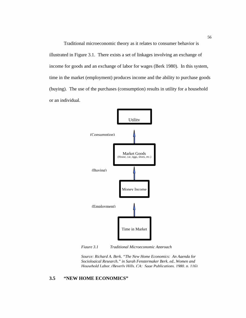
56
Traditional microeconomic theory as it relates to consumer behavior is
illustrated in Figure 3.1. There exists a set of linkages involving an exchange of
income for goods and an exchange of labor for wages (Berk 1980). In this system,
time in the market (employment) produces income and the ability to purchase goods
(buying). The use of the purchases (consumption) results in utility for a household
or an individual.
Market Goods(House, car, eggs, shoes, etc.)
Utility
(Consumption)
Money Income
(Buying)
(Employment)
Time in Market
Figure 3.1 Traditional Microeconomic Approach
Source: Richard A. Berk, “The New Home Economics: An Agenda forSociological Research,” in Sarah Fenstermaker Berk, ed., Women andHousehold Labor, (Beverly Hills, CA: Sage Publications, 1980, p. 116)
3.5 “NEW HOME ECONOMICS”
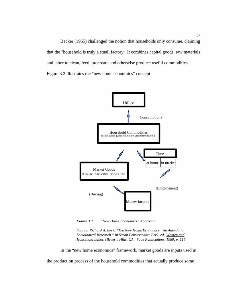
57
Becker (1965) challenged the notion that households only consume, claiming
that the "household is truly a small factory: It combines capital goods, raw materials
and labor to clean, feed, procreate and otherwise produce useful commodities".
Figure 3.2 illustrates the "new home economics” concept.
Household Commodities(Meal, tennis game, child care, attend movie, etc.)
Utility
Money Income
(Consumption)
Market Goods (House, car, eggs, shoes, etc.)
(Buying)
(Employment)
Time
at home in market
Figure 3.2 “New Home Economics” Approach
Source: Richard A. Berk, “The New Home Economics: An Agenda forSociological Research,” in Sarah Fenstermaker Berk, ed., Women andHousehold Labor, (Beverly Hills, CA: Sage Publications, 1980, p. 116)
In the “new home economics” framework, market goods are inputs used in
the production process of the household commodities that actually produce some

58
level of utility. A consumer's demand for market goods is a derived demand, in the
same manner that firms have a derived demand for the factors of production (Becker
1965). In this approach, time is spent either in the market (employment) or at home.
The time in the market produces income which is used to purchase goods (buying).
These goods are used at home to produce household commodities (consumption).
It is the process of combining goods and time at home that results in utility, rather
than the goods producing utility in their “raw” state.
The utility function described by Becker (1965) is as follows:
(3.3) Utility = u(Z1, Z2,....Zn)
where (Zi) stand for both the services from and the quantity of the commodity (Zi).
The commodity is produced by the household using a vector of market goods (xi )
and a vector of quantities of its own time (ti):
(3.4) Zi = zi(xi, ti, E)
where (E) is a vector of variables which represents the state of the art of production
or the level of technology of the production process. The utility function is
maximized subject to the production function constraints and a constraint on the
household's available time:
(3.5) T = tw + Sti
and an income constraint:
(3.6) I = Σpixi

59
where (tw) and (ti) are the household's time spent in the labor market and in
producing (Zi), and (pi) and (xi) are the price and quantity of the market-good input
used in producing (Zi).
The time and money income constraints are collapsed into a single resource
constraint on the household's "full income", (S).
(3.7) S = wT + V = Σ(wti + pixi)
where (w) is the wage rate, assumed to be constant, and (V) is the household's
nonwage income. The utility function (3.3) is maximized subject to the constraints
of the production functions (3.4, 3.5 and 3.6) and full income (3.7).
"By incorporating production concepts into the theory of consumption, the householdproduction function approach implies that households respond to changes in the pricesand productivities of factors, to changes in the relative shadow prices of commodities andto changes in their full income as they attempt to minimize their costs of production andto maximize their utility. A reduction in the price of some factor of production will shiftthe production process toward techniques that are more intensive in the use of that factorand toward commodities that use the factor relatively intensely. The theory of deriveddemand implies, for example, that the relative increase in the use of the factor will belarger the greater the elasticities of substitution in production and in consumption.
Likewise, if factor prices remain constant, an increase in the marginal productivity ofsome input induces several responses. To minimize costs of production, the factor'srelative use in the production process will increase. Since the relative price of thecommodity using this factor most intensively is reduced, the relative consumption of thiscommodity will increase. Since the rise in productivity raises full real income, thedemand for all "normal" commodities (those with positive income elasticities) willincrease. The absolute demand for the factor whose productivity rose will rise (or fall) ifthe combined effects of substitution in production and consumption and of expansionthrough the change in income outweigh (or are outweighed by) the productivity effectitself." (Becker 1976, pp. 139)
Becker’s (1965) formulation yields a marginal product of market goods
relative to a marginal product of time, which declines as the ratio of goods to time
rises. Thus, as money incomes rise, the relative decline in its marginal utility (or

60
marginal product) induces household members to conserve time and use money
relatively intensively. In other words, household members will be willing to spend
more money on products or services that produce a time savings, or make activity
choices that produce a time savings (such as trip chaining).
Becker’s contribution to the understanding of how individuals in households
make decisions using the construct of production theory, as he relates the activities
within a household to a firm. If transport is viewed as a factor that has become less
expensive (time reduction in travel due to increased supply of roadways), then more
of this factor (transport) will be used in the production process for an activity. If a
quantity of transport is used (the commute), and the resource “price” (both in terms
of time and money) remains constant, the increase in productivity of the use of
transport (more stops made between work and home) could result in an increase in
the use of transport. This additional use spreads the overall cost of travel over more
activities, thus, more is gained by using transport. The resulting increase in
productivity relates to an increase in full real income, which in turn could lead to the
purchase of more goods and services.
Pollack and Wachter (1975) extended Becker’s “new home economics”
approach, using a cost function C(P, Z), associated with the cost of the least
expensive collection of goods capable of producing the commodity vector (Z) when
goods prices are (P). However, they point out that when time is an input in the
household production process, joint production and increasing or decreasing returns

61
to scale are important to consider. Both of these conditions violate the functional
form used to describe household production. They agree that in the household
production function, utility is maximized rather than output. However, previous
work did not clarify when the production process stopped and utility began.
Graham and Greene (1984) looked at the issue of joint production as the
degree to which time devoted to home production simultaneously serves as a leisure
activity, particularly for women. Their findings suggest that it may not be possible
to distinguish activities in a discrete form.
3.6 HOUSEHOLD PRODUCTION APPROACH
“New home economics” addressed activities that were previously ignored
(home production activities), but did not include the ability to find substitutes for
these activities in the market place. In addition, it did not explicitly incorporate the
use of transport as an input into the production of activities.
The household production approach is based on the notion that time can be
divided into the portion spent in the market (employment) and out of the market
(see Figure 3.3). As previously illustrated in the “new home” approach,
employment generates income which is used to obtain goods (buying). These goods
are used at home to produce household commodities (consumption). It is the
process of combining goods and time at home that creates utility, rather than the
goods producing utility in their “raw” state.

62
It is also possible to obtain these “household commodities” in the market
place, using transport as an input and the income earned from market work. In
other words, a person can obtain utility (consumption) by traveling out of the home
and obtaining household commodities produced in the market place. The decision
to obtain household commodities in either of these conditions depends on which
activity location creates the greater utility.
It should be noted that transport is associated with most employment and
shopping activities. If transport is chosen as an input, then there is a derived
demand for travel as it relates to the production of that activity. Understanding the
underlying factors that increase or decrease the use of transport within a household
sets the stage for a better understanding of travel behavior.
There are a number of factors that have been associated with personal travel
behavior (Hanson and Hanson 1981). A major factor that influences the decision to
travel relates to the role of market work within a household. The amount of time
spent participating in market work impacts the total monetary resources available
for household consumption, the amount of time and the time of day available for
other activities, and the ability to accommodate for the needs of other individuals in
the household. As indicated in Figure 3.3, time spent in the market is generally
associated with a commute trip to work. However, market work can also be
conducted within the home in the form of telecommuting or home occupations.

63
Household Commoditiesout of the home
Utility
Money Income
(Consumption)
Market Goods(House, car, eggs, shoes, etc.)
(Buying)
(Employment)
Transport
Household Commoditiesin the home
+
Time
out of market
in market
Transport/Commute
Transport/Shopping
+
+
Figure 3.3 Household Production Approach
3.6.1 Monetary Influences
Total household income determines the monetary resources available to a
household for the purchase of goods and services. The number of workers in a
household and their marketable skills determines total household income. In
addition, the decision to work impacts the roles assigned within a household and
potential access to activity locations to and from work.

64
Gronau (1977) examined the relationship between time and money, using
wages and time in specific activities of individual members in a household, to explain
labor force participation of household members. His model was based on the notion
that there is a distinction between work at home (home production) and leisure
(home consumption). Home production is something that one would rather have
somebody else do (if the price is right), while it would be impossible for someone
else to enjoy your leisure. This presumes that home production generates services
which have a close substitute in the market.
Gronau’s (1977) simple model is based on a single-person household in
which the person maximizes the amount of some commodity (Z), which is a
combination of goods and services (X) and consumption of time (L)
(3.8) Z = Z(X, L).
The composition of (X) does not affect (Z), therefore, it makes no difference
whether a good is purchased from the market place or produced at home. Gronau
(1977) measured the value of the home goods and services (Xh) in terms of their
market equivalents. (Xm) represents market expenditures. Thus total consumption
is composed as:
(3.9) X = Xm + Xh.
Goods produced at home are subject to decreasing marginal productivity. This
decline in the value of marginal productivity at home is due not only to fatigue or
changes in input proportions, but also to a change in the composition of (Xh), a shift

65
toward activities that have a cheaper market substitute. The maximization of (Z) is
bounded by two constraints: the endogenous budget constraint,
(3.10) Xm = WN + V
where (W) is the person’s wage rate, (N) is hours of market work, (V) represents
other sources of income; and the time constraint,
(3.11) L + H + N = T
where (H) is the time spent in the production of home goods at home.
In Gronau’s paradigm, the more time an individual spends working at home,
the greater amount of home goods can be produced. If a person spends all his/her
time in work at home, some amount of homemade goods will be produced. Without
a market for homemade goods, this set is constrained. However, in the market
place, this constraint does not exist, in the sense that a person can sell his/her
working time and buy market goods. Thus, given the real wage rate (W), a person
can trade his/her time for goods along some price line. If this person chooses not to
work in the market place, he/she can spend time in leisure and/or housework. If the
marginal productivity of housework falls below the real wage rate, economic theory
would suggest that there will be no home production.
The implications of Gronau’s (1977) work is that as real wages increase, it
becomes less productive to conduct home production activities at home. It becomes
more productive to work in the market place and buy home production
“substitutes”. The travel induced by a decision to work includes the commute and

66
the subsequent travel associated with purchasing home production substitutes out of
the home. It should also be noted that increased productivity at home may reduce
the number of hours of labor needed in the market and raise real income as well.
Gronau (1977) considered the effect on activity participation resulting from
an increase in real wages. He found that if the real wage is increased, this change
affects both the rate of substitution between leisure time, the purchase of goods, and
the profitability of home production. The increase in wages lowers the price of
goods in terms of time, so home production is less profitable and induces
substitution of goods for leisure. Thus, this change will reduce home production
activities conducted in the home, while its effect on leisure is indeterminate. Home
production substitutes in the market place can be predicted to be used more
intensely. However, it is not possible to determine leisure activity participation.
Gronau also noted that work in the market involves costs, in terms of both
money and time. He referred to these costs as “fixed” in the sense that they are
independent of the amount of work performed (i. e., transportation costs and time.)
A person can stay out of the labor force, perform home production activities, and
save these costs. On the other hand, a person can choose to work and incur these
costs, at the same time, increasing total household income.
The influence of income levels on home production activities has been
examined regarding the purchase of prepared foods and meals prepared at home.
According to Redman (1980), a household's expenditure on ready-prepared foods

67
and meals away from home is inversely related to the amount of woman's time
allocated to household production. She found that family income had a positive
effect on meals consumed away from home. The fact that a woman worked out of
the home was not found to be significant.
Lamm (1982) found that the share of purchased meals of a consumer's
budget has increased relative to the share of a consumer's at-home food
expenditures. Using a translog approximation, he estimated the elasticities for food
consumed at home and for purchased meals to be highly inelastic, both with respect
to price and to total food expenditures. On the other hand, he found that non-food
items were both elastic for price and expenditures. However, the demand for
purchased meals is more elastic with respect to price and to total expenditures than
is the demand for food consumed at home.
Kooreman and Kapteyn (1987) found that unearned income had very little
effect on time use. An increase in the real wage rate of one of the members of the
household reduced the profitability of work at home by their partner, whereas the
effect on leisure activities was indeterminate.
In summary, total household income and the decision to work in the market
place will impact whether household commodities are produced and consumed in
the home or out of the home. However, it should be noted that wages and labor
productivity must also be considered. The number of workers in a household also
involves preferences of time use by the individuals within the household.

68
3.6.2 Temporal Influences
There are two elements to consider with respect to time. The first element is
the amount of time available for activities. The second element is the time of day
when an activity occurs. The more time one activity consumes, the less time is
available for other activities. In the same sense, ordering or scheduling activities
efficiently allows for participation in more activities or longer durations of choosen
activities.
Trip chaining increases the number of activities that can be participated in by
reducing the amount of transport used between activities. Downs (1992) points out
that many non-work trips are concentrated in the peak commuting periods as people
take children to school or run errands before and after work. In 1983, weekday
non-work trips made up 49.7% of all morning peak-hour trips and 68.9% of all
evening peak-hour trips (Downs 1992).
Gordon et al. (1988) found that between 1977 and 1983, non-work trips
grew faster than commute trips and grew during peak periods. Richardson and
Gordon (1989) found that the overall growth in non-work travel accounted for 70
to 75% of all week-day trips. They found that in all size SMSAs, nonwork travel
grew three to four times faster than work trips. They were unable to explain this
growth with traditional theories of travel. However, they made the assertion that
many of these non-work trips could be diverted to non-peak travel times.

69
Strathman, Dueker, and Davis (1993) used the concept of trip chaining to
examine the propensity of households to add non-work trips to the work commute
and the allocation of non-work trips through chaining. They found that workers
who commuted in peak periods had a lower propensity to form work/non-work
trips. They also found that certain household types contributed the largest amounts
of peak period chaining behavior: single adults; dual income couples; dual income
families with preschoolers; and multi-worker households. These types of
households were also the faster growing type of household formations.
Interestingly, a general congestion indicator had no effect on the allocation of non-
work trips among alternative chains.
Single occupant commuters had a higher propensity to add non-work trips to
their commute. Trip chaining analysis lead to the puzzling conclusion that even with
the increase of congestion during peak periods, people continued to trip chain. This
could indicate an inelastic demand for the activities/locations, regardless of the price
to be paid in congestion, both in time or money. It should also be noted that relative
time costs may actually be lower during the peak if congestion is increasing at all
times of the day.
Davidson (1991) examined the exact nature of trip chains in a study of
employees. The data defined a full work trip, including stops for meals, shopping
and daycare. The study found that the employees were twice as likely to make stops
on their way home from work as they were during the morning. Their chains had

70
the following compositions: morning chain - (45.2% ) gas, (22.7%) bank, (19.4)
dry cleaners, (16.4%) to eat; evening chain - gas (63%), shop (55.8%), bank
(49.6%) and dry cleaners (31.5%).
Hamed and Mannering (1993) found that travelers who depart from work
between 2:00 p.m. and 6:00 p.m. are less likely to be involved in a chain of
activities. Adler and Ben-Akiva (1979) included scheduling convenience in a utility
function for travel patterns. Small (1982) found that scheduling of trips was
affected by congestion. Noland and Small (1994) further determined that
uncertainty from unexpected, non-recurrent events contributed to the departure time
decision. Wilson (1989) found estimates of scheduling costs are higher than the
estimates for the value of travel time. Kitamura and Kermanshah (1983) found
evidence that past activity may impact current activity choice. Nishii, Kondo and
Kitamura (1988) report that the likelihood of choosing non-work activity in a
separate, home-based trip chain will increase with speed of travel and decrease as
commuting distance, travel cost, or density of opportunities increase.
Previous research has addressed the need to look at travel patterns during
specific time periods and to recognize that certain activities are occurring during
these periods. However, no clear pattern emerges on the relationship among
activity participation, the amounts of time available, and specific time periods during
the day.
3.6.3 Socio-demographic Influences

71
Socio-demographic characteristics have been associated with trip generation
and travel behaviors (Pas 1984). The general approach of determining the average
number of trips per household blurs more complex influences. Some of the socio-
demographic characteristics previously considered include gender, age, household
size and income.
3.6.3.1 Gender. There have been numerous studies indicating differences in travel
behaviors between women and men. However, there have been no systematic
studies looking at activities conducted in the home or out of the home with respect
to gender. Studies have looked at gender differences in the length of trips, mode
choice, trip purpose and miles traveled. For example, Wachs (1987) found women
made shorter work trips, used transit more than men, made more trips for the
purpose of providing travel services for others, and drove fewer miles than men.
Madden (1981) found that sex differences in household "roles" was the most
important factor in influencing women to work "closer to home" (make shorter
commute trips). McLafferty and Preston (1991) found that white women had
significantly shorter commuting times than white men. Among minorities, there was
no gender difference. Hanson and Hanson (1981) report that Swedish women who
worked, made more shopping and domestic trips, fewer social and leisure trips, and
used transit more than their spouses. Rosenbloom (1987) found women accepted
more responsibility for the travel needs of children. Bernard et al. (1996) found
women who worked made more trips than non-working women. Gordon, Kumar,

72
and Richardson (1989), using the Nationwide Personal Travel Survey (NPTS) data,
report that the growth of non-work trips-making is greater for women than men.
Hamed and Mannering (1993) found that males are more likely to go directly home
after work than females.
There appear to be no clear pattern between men and women with respect to
personal travel behaviors. Residential choice impacts the length, and to some
degree, the frequency of trips for market work, shopping, and other activities. The
complexity of household decision-making must be considered with respect to an
“optimal” residential location, given a complex set of constraints. It will be assumed
for purposes of this dissertation that utility maximization includes a residential
location that is consistent with the preferences of the household members.
3.6.3.2 Age. There is a general assumption that mobility declines with age. Bhat
(1998) found that older people were more likely to participate in in-home rather
than out-of-home activities. Abu-Eisheh and Mannering (1987) found that young
commuters tend to drive faster than older ones. In addition, older individuals were
less likely to participate in recreational activity than in social or shopping activities
(Damm 1980; Hamed and Mannering 1993). It should be noted that personal travel
behaviors also reflect cultural norms for particular age cohorts. In other words, the
preferences indicated by the elderly today may be specific to their generation. This
makes is difficult to assume that the elderly population of the future will behave in a
similar manner. It should also be noted that physical impairments associated with

73
aging may reduce mobility, regardless of the desire of certain individuals to remain
active and mobile.
3.6.3.3 Household structure. The structure of a household may affect the initial
decision to travel and the amount of time spent participating in various activities
(Gordon et al. 1994; Gramm 1975). A proxy for household structure is household
composition, including the number of children and their ages. Gronau (1977)
looked at the effects on time use of an increase in the number of children and their
age cohorts and found that as the number of children in a household increases,
additional of time will be devoted to work at home and leisure. He also contends
that child-care are less leisure intensive than other activities. An increase in the
number of children, at the expense of other activities, should reduce a parent's
leisure time. The effect of children on work at home and in the market depends on
the profitability of home production.
One parent may receive a lower wage than the other and may also be more
productive in home production activities. An increase in the number of children,
therefore, should lead to that parent spending less time involved in market work
(including commuting) and more time at home. The scope for profitable child-
related home production may be more limited for the other parent. In other words,
the presence of children generally results in one parent transferring time from the
market place to tasks performed in the home.

74
According to Gronau (1977), there is an assumption that a mother entering
the work force faces costs, such as child-care, that exceed the husband's cost of
entry. However, such costs are associated with the wife's work in the same way as
the gardener is with a working husband. Unlike expenditures like commuting costs
and time, which are prerequisites for work, they are costs which the family is willing
to undertake assuming that it is unprofitable for the wife to spend her time in child-
care activities at home.
Redman (1980) found that increasing household size had a negative effect on
meals being eaten outside of the home. Households with preschool children spent
significantly less on meals out of the home than other households. As the children
aged, more money was spent on meals out of the home. She also found that older
women spent less money on meals out of the home than younger women.
Households in metropolitan areas spent more money on meals out of the home than
rural households.
Miller (1993) found that having pre-school children limits the time available
for work, leading to more part-time work, unless child care is purchased.
However, children are costly and may require additional earnings. If part-time
work is easier to obtain more quickly than full-time work, temporary decreases in
normal income sources may be supplemented by part-time work.
Kooreman and Kapteyn (1987) found that in two-earner households, the
presence of young children reduced the amount of time spent by the wives on

75
leisure activities (defined as entertainment and social activity). The husband’s time
allocations were barely affected by the presence of children. Hamed and Mannering
(1993) found that stay-home durations were negatively impacted as the number of
children increased out-of-home activity participation.
The decision of a mother to go to work (requiring a commute trip and a day-
care stop) appears to be dependent on the real wage she faces, her productivity at
home, and the age of the children in the household. Household size affects the
decision to work, the status of that employment (i.e. full-time or part-time) and
impacts the time available for other activities.
Another important element of household structure is the marital status of the
adults. Gronau (1977) found that single men performed less market work than
married men. Married women, in his study, spent more time than unmarried women
in work at home. Kohlhase (1986) found that married women decreased their
participation in market work when wages were increased, while single women
increased their hours of work. She points out that aggregate studies which ignore
the differences in demographic structure are likely to misrepresent overall behaviors.
Koppelman and Townsend (1987) examined the construct that travel/activity
behavior of individuals is not only related to his/her own needs and desires, but to
the needs and desires of the household. They looked at the theoretical trade-offs
between components of time spent in working at home (home production). They
76
found that increasing the relative power of one person in a household decreased that
persons time in home and market work and increased their time in leisure, while
having the opposite consequences for the other person in the household. There was
no direct relationship between time spent in home-related work and market work.
Household structure also includes interdependencies across household
members. Gronau (1977) found that an increase in the wife's wage rate increased
her hours of work and reduced both her work at home and leisure time. This
change did not affect her husband's hours of market work, but was positively
correlated with his work at home and, as a result, negatively correlated with his
leisure time. An increase in the husband's wage rate increased his hours of work
(mainly at the expense of his work at home), but reduced his wife's market hours.
This change did not affect the wife's work at home, and consequently, it increased
her leisure time. An increase in unearned income reduced the hours of market work
for both husband and wife. In addition, it reduced work at home for the wife and
increases leisure time.
This work points out two important issues. The first issue is whether the
number of workers (commuters) is related to the wage rate faced by all the adult
household members. The second issue involves the importance of looking at the
individual household member’s contribution to total household income. Clearly,
taking the total household income as a predictor of household behavior masks the

77
importance of time use by individual household members and the allocation of
activities across members within the household.
According to Wales and Woodland (1977), as income increases, the
household may move to a larger house, requiring more time to be spent on
housework. However, the household might purchase more labor-saving appliances,
suggesting that housework time, depends on income and that it may or may not be
positive. Also, hours spent on housework by the husband and by the wife, are
neither perfect substitutes for each other, nor do they necessarily stand in fixed
proportion. Therefore, the allocation of housework time between the spouses may
depend on relative wage rates.
James (1996) looked at differences in what individuals perceive as their
“value” of home production activities, depending on whether they consider the time
spent in the activity to be an opportunity cost (the market value of their own time)
or at the market price (the amount they would have to pay someone else for the
service). He found that married women receive an additional $284 compared to
single men (opportunity cost method), or $4,012 more (market price), in value from
home production. Previously-married women receive relative to single men, $77
and $3,502 more from the opportunity cost and market price methods, respectively.
In addition, married men receive relative to single men, an additional $173 more
using the opportunity cost approach, while losing approximately $1,213 using the
market price method. These results indicate that the use of the opportunity cost

78
method results in relatively higher estimates of household production for men than
for women. At the same time, using the market price method, had the opposite
effect.
Blau and Ferber (1992) developed a model to examine the role of
specialization and exchange for a married couple. Their approach allows for a better
understanding of some of the economic realities facing a household and the resulting
impacts on personal travel behaviors. In their model, they assumed that individuals
derive utility from only two types of goods: home goods (produced with inputs of
home time) and market goods (purchased with market income). In a two-person
household, each person can allocate their time between housework and market
work. If each person is dependent on their own output, their production possibility
frontiers limit their consumption opportunities. If the individuals combine their
efforts, their combined production possibility frontier is greater than the sum of the
single frontiers. The difference, the gains from specialization and exchange, requires
them to produce non-trivial amounts of both market- and home-produced goods.
The authors point out that the gains from specialization are greater, the more
the two individuals differ in their comparative advantages. If each individual
produces the same set of goods, their combined per capita production equals their
individual production. In other words, there appears to be no gains realized.
However, there may still be some gains available as the two people can use many
goods and services more efficiently than single individuals.

79
Blau and Ferber (1992) suggest that the couples tastes play a role in how
they will ultimately determine how to allocate their time and income between home
goods and market goods. Using indifference curves, the authors note that if a
couple has relatively steep indifference curves, indicating a higher value being placed
on home goods, compared to market goods, it would take a larger amount of
market goods to induce them to give up a dollar’s worth of home goods while
remaining equally well off. Thus, to determine the allocation of time within a
household, the division of labor will be dependent on the production possibility
frontiers of the individuals and their tastes.
Consider a household where the wife has a comparative advantage in the
production of home goods, and the husband has a comparative advantage in market
work. If the couple has a relatively strong preference for market goods, in order to
maximize the household utility, the husband would specialize entirely in market
work, the wife would do all the household and some market work. In a household
that prefers home-produced goods, the wife would do only home production, and
the husband would also do some home production and market work. This set of
preferences would impact the amount of personal travel used within the household.
It is not clear, however, whether more or less travel would result as there may be a
greater need for travel for shopping activities and/or leisure activities.
Using the theory of comparative advantage, one individual can be said to
have a comparative advantage over another in the production of a particular good

80
relative to other goods they can produce, if they produce that good least inefficiently
as compared with the other person. In other words, if the wife produces the home
goods, all market work being equal, she also has the comparative advantage, if she
produces them least inefficiently compared to the husband. In addition, the greater
the difference between the two in their comparative advantage, the greater the gains
from specialization and exchange. At the same time, the greater the similarities in
their skills, the less can be gained by forming a household.
Household structure, in terms of roles and household decision-making for
married couples and the allocation of resources, has been addressed with several
models, including a bargaining model (Manser and Brown 1993) and a separate
spheres bargaining and marriage markets model (Lundberg and Pollak 1993). There
appears to be little research on household decision-making among nontraditional
couples. In addition, as Pisarski (1996) points out, the fastest growing household
type is the non-family household, increasing by 30% between 1980 and 1990. It is
unclear how the adults within these households interact with regards to activities, if
at all. Individuals in new household types, such as co-housing residents, may have
expectations of joint participation for some activities.
3.6.3.4 Years in the Home. It can be hypothesized that participation in some
activities, such as home maintenance, would increase the longer a person lived in the
same house. It is unclear whether the length of time at a particular residence should
be associated with a desire to conduct substitutable activities in or out of the home.

81
It may also be the case that new residents find more activities of interest in the early
years within their home, preferring more activities out of the home, over time. It
should be noted that this dissertation is not distinguishing between households that
rent and those that own their residence. This approach ignores the possibility that
there may be some set of activities that only home owners or only renters must
conduct.
3.6.3.5 Employment Status. As mentioned previously, when individuals spend
time at work, they have less time for other activities. Employment status, (full-time
or part-time work), may have different effects on an individuals ability to
participate in home production and leisure activities. According to Miller (1993),
part-time work is preferred by women combining market work with household
production when she has pre-school age children, during the years of family
formation. Part-time work is concentrated within unskilled occupations providing
limited access to training and advancement. As a result, real hourly wages paid to
part-time workers are lower than those obtained by full-time female workers.
There is a greater association with part-time and no market work than part-time
and full-time work.
Miller (1993) claimed that part-time work is closely associated with some
change in a household, such as the birth of a child, loss of spouses’ job, etc.
Previous research has determined that current labor market status is a good
predictor of future labor market behavior. However, it is not a static condition and

82
can change with unexpected changes. Unexpected events impact household
incomes and alter an individual’s taste for leisure.
Miller (1993) points out that women who work part-time have a greater
probability of continuing in part-time work. Women with tastes for market work
tend to develop careers in full-time positions. Thus, part-time work increases the
probability of continued part-time work. Pazy et al. (1996) found that mothers with
young children worked less hours a week and had lower career orientation. They
also found that single women worked closer to home compared to married women.
They considered single women to be more mobile in their residence choices,
enabling them to locate closer to work.
During child-bearing years, women who did not previously plan a full-time
career will become part-time workers and continue as part-time workers. Although
part-time workers have more flexible work schedules, they must also travel during
peak periods with obligations, such as taking children to school or if they begin or
end a work day during the peak.
3.6.3.6 Total Household Income. Household income has been included as an
important variable by transportation planners with respect to trips produced within
a zone (Khisty and Lall 1998). Although the stated purpose of the inclusion of total
household income is to reflect the behavior of trip makers, it is unclear whether the
parameters generated actually are representative of the intended population, given
the methods used to collect and manipulate the data. This is particularly true in

83
cities where there is evidence of mixed use urban form and mixed income
neighborhoods.
It is important to account for the number of persons within a household with
respect to the income available. For example, a one-person household with a
household income of $30,000 faces a different set of constraints than a household of
four with the same total income. However, it may not be appropriate to assume that
a per capita allocation of the resources across household members is needed. The
opportunity for economies of scale in larger households and differences in resource
needs by age may require a more detailed allocation model.
Personal travel behaviors are assumed to vary over different income levels.
For this dissertation, income levels will be considered in terms of low income (less
than $25,000), middle income ($25,000 to $60,000), and high income (above
$60,000). This approach to the selection of income groups may result in some loss
of information that might be available using more groups or different levels. Wage
data will not be used, however, the importance of wage levels must be considered.
3.6.3.7 Vehicles per Household. There have been a number of studies looking at the
influence of vehicle availability on travel patterns. It should be noted that
individuals may purchase vehicles in order to increase their mobility. The question
arises as to whether their propensity to travel is a cause or a result of the number of
vehicles owned. Meurs (1993) found that the demand for a second vehicle was
more elastic than for the first vehicle. Bhat and Koppelman (1993) reported that the

84
propensity for auto ownership was reduced with the presence of children and by
living in a large metropolitan area. Hamed and Mannering (1993) found that vehicle
availability increased the flexibility associated with postponing activities. Nobile et
al. (1996) used a random effects multinomial probit to better understand household
vehicle ownership patterns. They found that most of the variability in the observed
choices was associated with between-household differences rather than within-
household random disturbances.
Pisarski (1996) indicates that the number of vehicles now exceeds the
number of licensed drivers. The ability to afford additional vehicles may be highly
correlated with total household income, acting as a proxy for wealth. There may
also be a specialization process in the household fleet. For example, Golob et al.
(1994) looked at the use of vehicles in two-vehicle households. They included a
variety of vehicle types in their analysis, finding that subcompact cars are driven
more as either the first or second vehicle in the household. However, if the second
vehicle is a subcompact, the first vehicle is also driven more miles. More research is
needed on household fleet usage as the fleet mix directly impacts air quality.
3.6.4 Activity Location Decisions
If the utility of a “substitutable” activity conducted out of the home is greater
than that activity conducted in the home, then it is assumed that the activity will
include some input of transport and that some form of transport is available. The
exact distance required to conduct the activity is dependent on the built landscape.

85
The form of transport is dependent on the modes available at a particular time and
location to an individual household member. This dissertation looks only at the
decision to conduct a substitutable activity out of the home, however, this decision
is being made within the context of actual locations and modes available.
Previous studies have attempted to understand the nature of the decision to
conduct activities out of the home. For example, Kitamura (1984a) developed a
model of daily time allocation to discretionary out-of-home activities, using a utility
function that captured diminishing marginal utility. This utility was a function of the
activity duration and exogenous variables. As an extension to this concept, he
developed a discrete activity participation model based on the utility obtained by the
continuous time allocation model. The model attempts to determine the optimal
activity duration for out-of-home and in-home activities.
According to Schor (1992), in some households, women are able to
substitute commercial services for their own labor, using their newly earned
paychecks to pay the bill. Expenditures on these home production substitutes, such
as precooked food (either restaurants or from the neighborhood deli), professional
child care, and dry cleaning, have risen rapidly in recent years. There is a self-
reinforcing nature to this process as the growing demand for commercially produced
products draws more women into service sector employment. Once employed, time
constraints increase, as does the likelihood of a home production substitute being

86
chosen. It is not clear, however, what effect this substitution has on the travel
patterns of individual household members.
Gronau (1986) points out that "cooking time" and "driving time" are
substitutes to the extent that "eating at home" and "eating out" are substitutes, and
"eating out" and "going to a play" are complements. Supernak (1982) states that an
out-of-home activity is selected only if it is "better" at a given time than some
competing home activity. An out-of-home activity is often referred to as having a
disutility associated with the travel component of the activity. In-home activities
may also have elements of disutility (i.e. preparatory work).
Kitamura (1988) points out that in-home/out-of-home activity substitution
does not uniquely determine travel demand because in-home activities also generate
trips. He also notes that activity data is cross-sectional time use data and reflects
differences in time use across individuals, but not substitution between in-home/out-
of-home activities for a given individual.
Without a clearer understanding of the use of transport within the context of
household travel/activity decisions, travel forecasting models lack adequate
sensitivity to changes that household members might make under new or different
conditions. This dissertation looks at the factors assumed to impact the decision to
conduct a substitutable activity out of the home. It should be noted that
substitutable activities conducted out of the home are responsible for only a portion

87
of the trips that are generated by a household. The household production approach
may also be useful for additional personal travel decisions in future research.
3.7 SUMMARY
Microeconomic principles provide a framework for understanding the
derived demand for travel. Traditional consumer theory, based on utility
maximization, has been extended in the development of “new home economics”. In
this construct, utility is derived from the production of goods within the home.
However, individual household members may be able to maximize utility from two
sources. One source is through the production of household commodities within the
home and the other is from the purchase of household commodities out of the home.
Transport is necessary to obtain these “substitute” household commodities. A
household production approach provides a framework to explain the travel behavior
differences using socio-demographic characteristics associated with the choice of an
activity being conducted in or out of the home. These socio-demographic factors
include gender, age, household structure, years spent living in a home, employment
status, total household income, and number of vehicles in the household.
Increases in age, household structure, and years spent living in the same
house are expected to decrease the amount of “substitutable” activities conducted
out of the home. Being employed, having a higher household income and owning
more vehicles are expected to increase the number of these activities conducted out

88
of the home. It is unclear whether men or women are more likely to conduct these
activities out of the home. In addition, the time of day that activities are conducted
may result in some activities being conducted out of the home rather than in the
home.

89
CHAPTER FOUR
HOUSEHOLD TRAVEL/ACTIVITYDECISIONS: A CONCEPTUALMODEL
4.1 INTRODUCTION
The concept of utility maximization is founded on a set of economic
principles that will be useful in explaining household travel/activity decisions.
Within the context of a household production function, individual household
members obtain utility from household commodities produced within the home or
purchased out of the home. The concept of utility maximization within a household
can be generalized to a set of activities that can be conducted either in or out of the
home. The choice indicates which location is preferred. Utility maximization is
generally expressed in terms of a function and a set of constraints.

90
4.2 CONCEPTUAL MODEL
In a simple framework, a household members’ utility is a function of a set of
activities conducted in or out of the home:
(4.1) U = f(AH, AO)
where (U) is the utility obtained participating in the activities. (AH ) are the activities
conducted in the home. (AO) are the activities conducted out of the home. The
individual will derive the greatest utility by choosing a set of these activities which
maximizes the his/her overall utility function, subject to a monetary resource
constraint for the household represented by:
(4.2) Y = PH*AH + PO*AO
where (Y) is the total household income, (PH) is the monetary resource price of
conducting an activity in the home, and (PO) is the monetary resource price of
conducting an activity out of the home.
The Lagrangian equation for the optimization problem is as follows:
(4.3) L = U(AH, AO) + λ(Y- PHAH - POAO)
The first order conditions are:
(4.4) LH : UH - λPH = 0 LH : δU/δAH - λPH = 0 LH : δU/δAH = λPH
(4.5) LO : UO - λPO = 0 LO : δU/δAO- λPO = 0 LO : δU/δAO = λPO
(4.6) L λ : Y - PHAH - POAO = 0
(4.7) UH / UO = PH /PO

91
This would suggest that the ratio of the marginal utilities of activity locations (in or
out of the home) is equal to the ratio of the monetary resource prices for these
activities. Characterizing the choice to conduct an activity in or out of the home in
this manner ignores the fact that individuals face additional constraints associated
with the decision of where an activity will be conducted.
Consider the constraint associated with spatial opportunities, where (D) is a
function of distance with respect to activities in the home (AH) and activities out of
the home (AO):
(4.8) D(AH, AO)
This represents an understanding that the distance that an individual is willing to
travel is a function of a chosen activity. The spatial opportunity set for a given
activity can be defined as those locations within this activity space. By expressing
distance as a function of an activity, it is possible to consider different spatial sets,
associated with discrete activity types.
In an extended conceptual model, goods required for an activity in the home
must be gathered through prior shopping. The gathering of these goods is
represented in the equation as D(AH), the distance traveled as a function of an in-
home activity. For activities conducted in the home that require no market inputs,
D(AH), the spatial component, equals zero.
Traditional trip analysis encompasses the results associated with D(AH, AO),
the decision to travel to participate in an activity. The conventional approach views

92
each trip as a separate entity, often ignoring stops for activities between home and
work. As mentioned previously, there are spatial economies to be gained through
chaining activities together. The ability to reduce these distances influences the
marginal utility associated with an activity.
By making distance a function of an activity choice, the feasible set of
locations or accessible options are located within some explicit limit. McNally
(1998) has developed a Geographical Information Systems (GIS) representation of
the ambient density of potential activity locations dependent on the current location
and the transportation network for the mode being utilized. One important point
with regards to distance is the idiosyncratic nature of the built landscape and the
modes available for use. This dissertation does not explicitly use the geocoded form
of the Oregon and Southwest Washington 1994 Activity and Travel Behavior
Survey activity data. Further research to incorporate specific geocoded information
will be needed in order to explicitly quantify the model. Hubbard’s (1978) criticism
of previous work on consumer travel behavior, suggests that this line of research
will be able shed light on the debate over the effects of urban form on travel.
There is a temporal constraint, (H), which is a function of time with respect
to activities in the home (AH) and out of the home (AO):
(4.9) H(AH, AO)
In other words, the time an individual is willing to spend participating in an activity
is a function of that activity, either conducted in or out of the home. Previous

93
research portrayed an activity as being dependent on the time available. By
describing time as a function of an activity choice, it is not as important to
predetermine if an individual is required to spend some specific limited amount of
time at an activity or is choosing to spend as much time as desired. The decision
becomes part of the function for a particular activity.
The time component, H(AH, AO ), includes the travel time necessary to gather
goods and to conduct an activity. Again, for activities that require no market inputs,
H(AH), represents only the activity participation duration in the home. Further
research incorporating Wang’s (1996) timing utilities and Doherty’s (1998) ability
to examine flexibility in activity scheduling may guide the development of the
appropriate functional form, with respect to time constraints.
The Lagrangian equation for this activity/travel problem is as follows:
(4.10) L = U(AH, AO) + λ(Y- PHAH - POAO ) + φ(D(AH, AO)) + ψ(H(AH, AO))
(4.11) UH = λPH - φDH - ψHH
(4.12) UO = λPO - φDO - ψHO
(4.13) UH /UO = λPH - φDH - ψHH / λPO - φDO - ψHO
The equation states that the ratio of the marginal utility of conducting an
activity in the home to the marginal utility of conducting a “substitute” activity out
of the home is equal to the ratio of the respective nominal prices, travel costs, and
time costs, weighted by the appropriate Lagrangian multipliers. In those instances
where an individual chooses to conduct an activity out of the home, the marginal

94
utility with respect to the three components must necessarily be greater than
conducting the activity at home.
It is also the case that the contribution of any of these factors can be the
determining element in the decision. For example, Evans (1972) suggested that
higher income individuals may be less affected by an income constraint than
individuals from lower income households. In other words, it would be incorrect to
assume that any one factor (income, distance or time) alone, explains household
travel/activity decisions for all groups. In addition, DeSerpa (1971) points out that
time constraints can have different consequences depending on whether time is
considered a resource or a commodity. When the spatial component, or accessibility
space, is combined with scarce time resources, the decision to link activities together
(trip chain) becomes more compelling. This is particularly true for a person who is
already traveling between home and work (the commute trip).
An example of how the three components (the nominal price component, the
spatial component, and the temporal component) guide the understanding of the
household travel/activity decision can be illustrated using the decision of where to
eat a meal. In a one-person household, the price of the market goods for a meal, the
distance to travel and participation time to shop, the preparation and clean-up time,
and the time to consume a meal will be evaluated at the margin with the price of a
prepared meal, the travel time (which may be combined with a commute trip), and

95
the consumption time for the meal. In the case of single men, the utility of eating
out will most likely be greater than eating at home.
Extending the conceptual model from a one- to a two-person household
presents the challenge of determining the functional form of an overall “household
utility function” that incorporates the individual utility functions of each person. For
example, consider an overall utility function for a two-person household:
(4.14) UHH [ U1(AH1, AO1), U2 (AH2, AO2)]
The first order condition for an activity conducted out of the home is:
(4.15) dL/dAO1 = [δUHH/δU1 * δU1/δAO1] = UHHAO1
where (UHHAO1 ) represents the individual marginal contribution to the overall
household utility of participating in an activity conducted out of the home.
This conceptualization of a household utility maximizing function should illustrate
why a person in a single person household might make a different set of choices than
that same individual would make as a member of a multi-person household. The
exact nature of such relationships within the household, remains problematic. There
is some concern that utility functions across individuals are not additive. A possible
Lagrangian equation for an individual in a two-person household is as follows:
(4.16) L = U1(AH1, AO1) + λ(Y1- PH1AH1 - PO1AO1 ) + φ(D(AH1, AO1)) +ψ(H(AH1, AO1)) + γ[U2(AH2, AO2) + α(Y2- PH2AH2 - PO2AO2 ) +ω(D(AH2, AO2)) + θ(H(AH2, AO2)) - U2]
where
(4.17) Y = Y1 + Y2 + S

96
In this case, the first household member will maximize his/her utility, given the
constraint of not reducing some preassigned utility U2 of the second household
member. There is an additional requirement that the income portions Y1, Y2 and
any additional unused portion of income that represents savings S, sum to the total
household income Y. However, this representation does not characterize the
interdependent nature of activities within the context of a multi-person household.
For each person in the household, there is a set of activities that can be
considered private activities, where the value of activity participation is captured
completely by that individual. There is another set of activities that can be
characterized as household-oriented activities, that is, activities that influence the
utility of other members of the household. In some respects, household-oriented
activities have the characteristics of non-exclusive public goods.
Consider a two-person household, where the utility of person one (U1) is
comprised of the activities chosen for private consumption, X1(AH, AO), another set
of household activities conducted by person one for the benefit of all household
members, including him/herself, Z1(AH ,AO), and household activities conducted by
person two that can include person one and therefore are some portion of the
household activities participated in by person one, αZ2(AH, AO). Equation (4.20),
introduces (F) as a representation of the overall household production function.
Thus,
(4.18) U1 = U1(X1, Z1 + αZ2)

97
(4.19) U2 = U2(X2, Z2 + βZ1)
(4.20) F(X1 + X2, Z1 + Z2) = 0
where 0 < α, β < 1.
To determine the conditions that will characterize an efficient allocation of
resources within the context of the household, a Pareto efficiency condition is
considered (Oates 1972). In this case, the utility of one household member is
maximized, while holding constant the utility of the other. The maximizing
expression, including the production constraint, is:
(4.21) L = U1(X1, Z1 + αZ2) + λ1[U2(X2, Z2 + βZ1) - U0
2] + λ2 [F(X1 + X2, Z1 + Z2)]
where λ1 and λ2 are Lagrangian multipliers and U02 is the second household
members’ given level of utility.
Under this specification, the first-order efficiency conditions are:
(4.22) MRT = MRS1 + βMRS2 = αMRS1 + MRS2
Thus, the marginal rate of transformation (MRT) of private activities for household-
oriented activities for/with other household members, must equal the sum of the
marginal rates of substitution for each person. The special case for equation (4.22)
where the participation parameters are equal to zero (α = β = 0), occurs when all
activities are private (i.e., a one-person household). In the special case where
α = β = 1, household activities are similar to pure Samuelsonian public goods and
the MRT equals the sum of the individuals MRS’s. However, the intermediate
condition is worth exploring in the context of household travel/activity decisions.

98
Equation (4.22) suggests that the joint benefit from participating in
household-oriented activities (Z), must be the same, regardless of which person
generates the marginal household-oriented activity. Following the notions presented
by Oates (1972), if this condition were not satisfied, it would be possible to increase
welfare by shifting more household-oriented time to that person whose participation
in household-oriented activities generates a greater joint gain. In addition, the
opportunity cost of an extra unit of household activity in terms of private activity
participation must equal the joint benefit, measured in terms of the amount of
private activity participation the individuals would be willing to give up for an
additional unit of household activity participation. In other words, the sum of the
benefits of an extra unit of household activity participation must equal its marginal
“cost”.
Oates (1972) uses the term, “spillin effects”, to describe the benefits received
when public goods are purchased by one jurisdication, but are available to others as
well. Although his work was applied to an understanding of reciprocal externalities
and a system of intergovernmental grants, it may also have application for the
behavior of individual members of a household. In a similar vein, household
members receive “spillin” benefits from participating in household activities
produced by another member.
According to neotraditional economic theory, a competitive arrangement
would generate an inefficient level of these “public good” household activities,

99
whereas a collective action strategy is more likely to approach an efficient level of
provision. The nature of a household more closely resembles a collective effort,
recognizing that the participation parameters may not be equal across household
members, as each member is choosing a preferred set of activities to maximize
his/her own utility.
In order to best insure receiving their desired portion of “spillin” benefits, a
household member must necessarily be in the company of other household members.
The choice of an activity location (in or out of the home) is therefore influenced by
this participation condition. The use of transport in a multi-person household
includes an additional component to capture “spillin” value. In other words, the use
of transport to participate in only private activities for an individual in a one-person
household, could differ greatly from the use of transport for a household member
who is trying to maximize utility from private activities, self-produced household-
oriented activities, and the household activities produced by other members. The
flexibility of reorganizing activities would be greater for individuals where all
activities have the characteristics of private activities.
Another area of concern is the role mode availability plays with respect to
the ability and desire to travel. It is certainly the case that accessibility of locations
for out-of-home activities is dependent on the modes available for travel. It is not
clear what effect assuming mode availability is exogenous rather than endogenous
has on household travel/activity decisions. It may be the case that individuals self-

100
select themselves into residential locations that provide the modes that they intend
to use to participate in activities. Although mode choice is often modeled using a
discrete choice or nested logit specification, it may not be appropriate to assume
that such decisions are sequential or independent decisions. This dissertation does
not address mode choice per se.
A third concern is the incorporation of the time of day when activities occur
into a utility maximizing framework. Previous research has indicated that peak
periods (morning and evening) are of interest to transportation researchers. Current
policy objectives and Tranportation Demand Management (TDM) programs aimed
at reducing congestion during these peak periods, may disturb or conflict with
household travel/activity patterns that maximize utility for individual household
members. In addition, it is possible to consider specific activities over a set of time
periods or participation in the same set of activities within a particular time period.
Developing the weights associated with income, space, time, and participation
constraints, will lead to a better understanding of the effects such policies have on an
overall household production function, on utility levels of individual household
members, and on groups of household types.
4.3 SUMMARY
The conceptual model of household travel/activity decisions allows for an
understanding of how different members of the same household and members of

101
different households may face a different set of constraints. The Lagrangian
multipliers indicate the various weights of the factors that impact household
travel/activity decisions. The addition of participation parameters help to explain
differences in the use of transport across households. Most importantly, a
household production approach illustrates that travel behavior may be based on a
more complex decision than the traditional approach of focussing on saving travel
time. Household members demonstrate their utility preferences in their personal
activity/travel behaviors by participating in a set of activities. Given a set of
observations and an underlying framework of household travel/activity decisions, it
should be possible to determine the impacts of various transportation policies on
individual household members and overall household utility.
CHAPTER FIVE
EMPIRICAL ANALYSIS
5.1 INTRODUCTION
The Portland Metropolitan Service District (METRO 1994) undertook a
comprehensive and innovative data collection program to support the development
of an improved travel demand modeling system. This data collection effort was one

102
of the first in the country to undertake a region-wide home interview survey
designed explicitly to support the development of a new generation of travel demand
models (Cambridge Systematics 1996). One of the unique features of the data is the
inclusion of activities conducted within the home.
5.2 DATA COLLECTION AND CLASSIFICATION
The data for this dissertation was collected using a region-wide, two day
activity survey. 4,451 households were surveyed by Metro, a regional governmental
agency in the Portland, Oregon, metropolitan area. The survey instrument, the
Oregon and Southwestern Washington 1994 Activity and Travel Behavior Survey,
was a detailed diary that recorded what each member in a household did (activity
choice), where (location choice), for how long (activity duration), and with whom
(activity participation). The recruitment rate (number of recruited households with
complete household and person data divided by the number of households eligible
for recruitment) was 53 percent. The completion rate (number of households
completing the survey process divided by the number of recruited households) was
63 percent, with an overall response rate of 33 percent. In the survey data, 9,471
persons reported 122,348 activities and 67,891 trips (Cambridge Systematics 1996).
An effort was made to “over-sample” the transit corridors in order to obtain survey
information from individuals must likely to use transit.

103
The individual descriptions of activities were categorized into 27 activities.
Only certain activities can be performed either in the home or out of the home. For
those activities that can only occur in one location (i.e., sleeping at home), the
decision to participate in that activity is generally location-specific. However, if
there is a choice of locations (including at home), the decision is more complex.
Golob and McNally (1995) aggregated the highly specific activities into
broad activity types (work, maintenance, and discretionary). An alternative broad
aggregation was developed which reclassified the data, such that work was
combined with school activities and meals were considered discretionary (Bowman
1998). A third set of categories (limited aggregation) combines these approaches in
order to disaggregate maintenance activities to allow a closer examination of
possible differences with respect to activity participation.
Table 5.1 lists three possible classification schemes.
Table 5.1 Classification Schemes for Activity Data
Description of Activities Aggregate Activities Limited Aggregation
Meals Discretionary MealsWork Work/School WorkWork-related Work/School WorkShopping (general) Maintenance activity ShoppingShopping (major) Maintenance activity ShoppingPersonal Services Maintenance activity Personal ServicesMedical care Maintenance activity Personal ServicesProfessional services Maintenance activity Professional servicesHousehold/personal business Maintenance activity Household/personal businessHousehold maintenance Maintenance activity Household maintenanceHousehold obligation Maintenance activity Household obligationPick-up/drop-off passenger Maintenance activity Pick-up/drop-off passengerVisiting Discretionary activity Discretionary activityCasual Entertaining Discretionary activity Discretionary activity

104
Formal Entertaining Discretionary activity Discretionary activitySchool Work/School SchoolCulture Discretionary activity Discretionary activityReligion/Civil Service Discretionary activity Discretionary activityCivic Discretionary activity Discretionary activityAmusements (at home) Discretionary activity Discretionary activityAmusements (away from home) Discretionary activity Discretionary activityHobbies Discretionary activity Discretionary activityExercise/Athletic Activity Discretionary activity Discretionary activityRest & Relaxation Discretionary activity Discretionary activitySpectator Athletic Event Discretionary activity Discretionary activityIncidental trip Discretionary activity Discretionary activityTag along trip Discretionary activity Discretionary activity
There is no standard aggregation with respect to activity-based data. As a
consequence, research outcomes may be more dependent on the data classifications
rather than the underlying research hypothesis being tested. For example, the
placement of meals as a discretionary activity rather than as a home production
activity resulted in differences in logit regressions coefficients (Lawson 1997).
Bernard et al. (1996) expressed a need for the development of a universal typology
for describing household structure, using activity-based data sets.
For the purposes of the initial examination of the data, an activity must occur
both in and out of the home to be considered “substitutable”.
Table 5.2 Classification of Activities that Occur Both In and Out of theHome
Activity Type Activity Description In-Home Out-of-Home
Work At office/plant, at home, on-site, performing thelabor, task or duty that is one’s means of livelihood.
1311(9%)
12693(91%)
Non-work All other activities (not including travel). Includeshome production and leisure activities.
52164(83%)
10909(17%)

105
HomeProduction
Activities associated with chores and duties related tohousehold functions. Includes meals, householdbusiness, maintenance, and obligations.
42958(85%)
7526(15%)
Meals Preparation or consumption of meals intended forhousehold members only.
18257(77%)
5575(23%)
HouseholdBusiness
Paying bills, banking, post office, etc. 676(34%)
1332(66%)
HouseholdMaintenance
Fixing, cleaning, laundry, etc. 8490(97%)
273(3%)
HouseholdObligation
Child care, baby needs, helping kids with homework,etc.
1535(82%)
346(18%)
Leisure Activities associated with relaxation. Includesexercise, rest & relaxation, and amusement activities.
23206(87%)
3383(13%)
Exercise Golfing, swimming, skiing, tennis, baseball, jogging,etc.
669(35%)
1239(65%)
Rest &Relaxation
Bike ride, stroll, out for a drive, etc 4398(93%)
322(7%)
Amusement TV, radio, videos, video games, movies, carnival,circus, nightclubs, etc.
18139(91%)
1822(9%)

106
Table 5.2 indicates the major categories of work and non-work, the subcategories of
non-work, home production and leisure, the individual activities that make up these
categories, and descriptions of what these activities entail.
5.3 CHI SQUARE ANALYSIS
The first step in determining the use of transport, within the context of
maximizing utility for household members, used a chi square analysis technique.
Only those persons 18 years of age or older were used in the analysis. Cross-
tabulations with chi-square statistical analysis were performed based on gender and
household size (proxy for children). Each activity type was analyzed separately to
determine differences in activity types.
5.3.1 Hypothesis One: There is no difference in activity location by activity type with respect to gender.
5.3.1.1 Place of Work. Respondents reported where they conducted market work,
in the home or out of the home. The majority worked out of the home, however,
there was a statistically significant difference between men and women (χ � = 5.5,
1, p < .05), with men more likely to do market work in the home and women more
likely to do market work out of the home.
5.3.1.2 Place of Meals. There was a statistically significant difference (χ � =
57.1,1, p < .0001) between men and women with respect to whether meals were

107
eaten in the home or out of the home. Men were more likely to eat out of the home
than women.
5.3.1.3 Place of Household Business. There was no significant difference between
men and women on whether they participated in household business in or out of the
home (χ � = 1.25, 1, p > .05).
5.3.1.4 Place of Household Maintenance. There was a significant difference
between men and women on the location of household maintenance activities (χ � =
37.4, 1, p < .0001). Men were more likely to do home maintenance activities out of
the home, while women were more likely to participate in the home.
5.3.1.5 Place of Household Obligations. There was no significant difference
between men and women on whether they participated in household obligations in
or out of the home (χ � = 1.26, 1, p > .05).
5.3.1.6 Place of Exercise. There was a significant difference between men and
women on the location of exercise activities (χ � = 25.47, 1, p < .0001). Men were
more likely to do exercise activities out of the home, while women were more likely
to participate in the home.
5.3.1.7 Place of Rest & Relaxation. There was no significant difference between
men and women on whether they participated in rest and relaxation in or out of the
home (χ � = .042, 1, p > .05).

108
5.3.1.8 Place of Amusement. There was no significant difference between men and
women with respect to the decision to conduct amusement activity in or out of the
home (χ � = .091, 1, p > .05).
These findings indicate that men are more likely than women to participate in
exercise or home maintenance activities out of the home. The fact that men were
more likely to eat meals out of the home may or may not generate new trips if they
are eating their meals while on their way to participate in some other out of the
home activity. Interestingly, men are more likely to work at home than women,
which might indicate that men are more capable of taking advantage of
telecommuting with their chosen occupations than women.
5.3.2 Hypothesis Two: There is no difference in activity location by activity type with respect to household size.
5.3.2.1 Place of Work. There was no significant difference in whether work was
conducted in or out of the home with respect to household size (χ � = 14.8, 7,
p > .01).
5.3.2.2 Place of Meals. There was a statistically significant difference in the
location of meals with respect to household size (χ � = 106.5, 7, p < .0001).
Households with one or two members were more likely to eat out. Households with
three or more individuals were more likely to eat at home.
5.3.2.3 Place of Household Business. There was no significant difference in
whether household business activities were conducted in or out of the home with
respect to household size (χ � = 18.3, 7, p > .01).

109
5.3.2.4 Place of Household Maintenance. There was no significant difference in the
choice of household business location with respect to household size (χ � = 14.3,
7, p > .01).
5.3.2.5 Place of Household Obligations. There was a statistically significant
difference in whether individuals participated in household obligations in or out of
the home with respect to household size (χ � = 21.8, 7, p < .01). Individuals from
one or two person households were more likely to participate in household
obligations out of the home, while those from households with three members were
more likely to do so in the home.
5.3.2.6 Place of Exercise. There is a significant difference across individuals based
on household size with respect to the location of exercise activities (χ � =19.9, 7, p
< .01). Households of one or two persons were more likely to exercise in the home.
Households of three or more members are more likely to participate in exercise out
of the home.
5.3.2.7 Place of Rest & Relaxation. There was no significant difference in whether
individuals participated in rest and relaxation in or out of the home based on
household size (χ � = 5.87, 7, p > .05).
5.3.2.8 Place of Amusement. There was a significant difference on the location of
amusement activities with respect to household size (χ � = 26.5, 7, p < .0001).
Individuals from one person households were more likely to participate in
amusement activities out of the home. Individuals in two person households were

110
more likely to participate in amusement at home. Individuals in households with
four or five members were more likely to participate in amusement activities out of
the home.
Both gender and household size do appear to have impacts on the decision
to conduct a substitutable activity out of the home. However, it should be noted
that these impacts appear to differ by activity type. For example, men are more
likely to perform market work at home. Home occupations and the use of
telecommuting options may be more desirable for men, based on their skill set and
other obligations. Men are also more likely to eat their meals, do their household
maintenance activities (i.e., laundry, chores), and participate in exercise activities out
of the home.
Household size effects differ for activities, such as meals, household
obligations, and amusement activities. One- and two-person households are more
likely to eat out of the home than larger households. In order for household
members in larger households to participate in this activity, the home location may
offer many advantages, including the ability to share the activity with other
members. Household obligations, such as childcare, are also more likely to be
conducted at home in larger households. Exercise and amusements, on the other
hand, are more likely to be conducted out of the home for larger households. Table
5.3 summarizes the findings of the chi square analysis.
Table 5.3 Summary of Statistically Significant Effects (p < .05)

111
Activity Type Activity Gender Household sizeWork Work/ Work-related Yes No differenceNon-workHome Production Meals Yes Yes
Household Business No difference No differenceHouseholdMaintenance
Yes No difference
HouseholdObligations
No difference Yes
Leisure Exercise Yes YesRest and Relaxation No difference No differenceAmusements No difference Yes
The empircial findings suggest that the decision to conduct substitutable
activities, such as meals and household obligations, are impacted by possible
“spillin” effects for larger households. However, chi square analysis does not
control for the effects of other factors, such as income, other time uses and
constraints, etc.
Another consideration is the effect of the availability of substitutes. For
example, as more mixed use development occur, commercial substitutes for home
production (fast food outlets, dry cleaning, etc.) become more convenient.
Accessibility of substitutes is also associated with various modes of travel. This
analysis uses cross-sectional data and therefore can not indicate changes in behavior
over time. It also did not use the geocoded data that locates activities spatially (see
McNally, 1998).
5.4 SUMMARY

112
The decision to participate in an activity out of the home, given that there is
a possible substitute location (in the home) for that activity, appears to be related to
gender and household size. Men are more likely to go out to eat and exercise, while
women are more likely to go out to work, suggesting that men are more likely to
telecommute than women or have home-based occupations.
Household size appears to influence decisions made by individuals,
indicating, perhaps, the concept of “spillin” effects. However, chi-square analysis is
a very limited form of analysis and only indicates a statistically significant difference
without offering any insight or additional understanding of the relationship. A more
sophisticated technique is needed to begin to understand the nature of the influences
on the decision to conduct a substitutable activity out of the home.

113
CHAPTER SIX
RANDOM UTILITY MODELS
6.1 INTRODUCTION
Activity-based household surveys contain information on what each member
in a household did (activity choice), where (location choice), for how long (activity
duration), and with whom (activity participation). The various factors that influence
the decision to conduct an activity in or out of the home can be examined using a
random utility model. This technique assumes that activity participation has been
determined prior to the decision to conduct an activity in or out of the home. Such
an assumption precludes recognition of the possible endogenous nature of activity
decisions. The research contribution made using this simplifying assumption is a
first step towards a better understanding of the decision to travel.
6.2 RANDOM UTILITY MODELS
The choice of whether to conduct an activity in or out of the home can be
characterized using random utility theory (RUT). RUT uses the notion that
behavior can be explained by recognizing a systematic and a random component in
the decision making process.
Thus,

114
(6.1) Ui = Vi + εi,
where (Ui) is the unobservable, yet true utility of alternative (i); (Vi) is the
observable or systematic component of utility; and (εi) is the random component. In
other words, (Vi) is the portion of the variance in a choice that can be explained and
(εi) is the portion that can not be explained. Although it can be assumed that there
will always be some portion of the variation that can not be explained, it is possible
to model or predict the probability that an individual will choose an alternative as
follows:
(6.2) P(i|C) = P[(Vi + εi) > (Vj + εj)], ∀ j ∈ C
where P(i|C) is the probability of choosing (i) from a set of competing alternatives,
defined as (C) (see Louviere, 1994). A random utility model can be used for an
activity conducted out of the home where (VO) and (VH) are the systematic
components of utility for conducting an activity out of the home and in the home,
respectively:
(6.3) P(i|C) = P[(VO + εO) > (VH + εH)], ∀ j ∈ C
The random component is assumed to follow a binomial distribution with a logistic
distribution for (ε) (Liao 1994). This also assumes the simplest probability model
form, with two response categories: event A or non-A.

115
6.3 LOGIT MODEL
6.3.1 Specification
A logit model is used to estimate the influence of variables on the decision to
conduct a substitutable activity out of the home. According to Demaris (1992), the
probability of an event occurring, Pi , can be expressed as:
(6.4) Pi = exp[α + β1
(X1
) + β2
(X2
) + ..βn(Xn)]/1 + exp[α + β1
(X1
) + β2
(X2
) + ...βn(Xn)]
Table 6.1 lists and defines the variables of interest.
Table 6.1 Socio-demographic VariablesVariable Mean Std. Dev. DefinitionP 0.2942 0.4557 Probability of Conducting an Activity Out of the HomeMALE 0.4731 0.4993 Gender (Male = 1) (Female = 0)AGE 48.0463 17.7894 Age ( > 18 years)HHS 2.5549 1.2620 Household SizeYRSR 4.0441 1.4132 Tenure of Residence (1= less than 6 months) (2 = 6
months, but less than 1 year) (3 = 1 to 5 years) (4 =more than 5 years, but less than 10 years) (5 = 10 to20 years) (6 = more than 20 years)
EMPLYD 0.6745 0.4686 Employed (Yes = 1) (No = 0)HHINC 0.1988 0.3991 Higher Income Household ( > $60,000)VEH 1.9399 1.0012 Number of Vehicles
The model uses a binary dependent variable for the choice of where a
substitutable activity is conducted (in or out of the home) and a set of independent
socio-demographic variables for an individual and his/her household:
(6.5) log(P/1-P) = f(MALE, AGE, HHS, YRSR, EMPLYD, HHINC, VEH);conditioned on activity type and time of day
The specification includes variables cited most frequently as influencing the
decision to travel. The primary motivation for using these variables is to determine
if they have a similar effect on the decision to conduct a “substitutable” activity out

116
of the home. It is not meant to be used as a travel forecasting model per se as it
obviously could have a number of omitted variables. It will, however, be of interest
to examine whether there are differences across activities with respect to the
influence of these variables. If all decisions to travel are influenced in a similar
manner by socio-demographic variables, then there should not be any statistically
significant differences across activities. In other words, the logit regression
coefficients should be the same, regardless of the particular activity chosen.
Differences across time periods can also be tested for effects.
The first logit regression examines all substitutable activities over an entire
day. Table 6.2 illustrates the effect of each variable on the probability of a
substitutable activity being conducted out of the home, either positively (+) or
negatively (-), for all substitutable activities, work, non-work, home production, and
leisure activities.
There are statistically significant differences in the effects of various factors
for all substitutable activities (Model 1). Being male, being employed, having a
household income greater than $60,000 and increasing in the number of vehicles per
household, all have a positive effect on the decision to conduct a substitutable
activity out of the home. Age, household size, and tenure of residence (years in
home), have a negative influence.

117
Table 6.2 Probability of Conducting an Activity Out of the Home for AllSubstitutable Activities and Major Groupings
Variable Model 1 Model 2 Model 3 Model 4 Model5
all activities work non-work homeproduction
leisure
Constant - - ++ -- - - - -MALE ++ + ++ ++ *AGE - - -- -- - - - -HHS - - * -- - - - -YRSR - - * - * *EMPLYED ++ N/A ++ ++ *HHINC (> $60,000) ++ * ++ ++ ++VEH ++ - ++ ++ ++
++ or - - indicates sign where p < .0001+ or - indicates sign where p < .01* indicates no statistical significance
When the data is disaggregated into work and non-work activities (Models 2
and 3), there are several differences of interest. Household size has a strong
negative influence for non-work activities and is not statistically significant with
respect to the work activity being conducted out of the home. Increasing the
number of vehicles per household has a negative effect on working out of the home.
When non-work activities are disaggregated into two major activity
groupings (home production and leisure), there are additional differences in these
effects. Being male is not statistically significant for leisure activities. However,
being male is positive and statistically significant for home production activities
conducted out of the home. Being employed is not statistically significant in the
leisure model. Home production and leisure activities are positively influenced by

118
employment. Table 6.3 reports the logit regression coefficients for Models 1
through 5.
Table 6.3 Probability of Conducting an Activity Out of the Home for AllSubstitutable Activities, Work, Non-work, Home Production andLeisure Activities Over an Entire Day (coefficients)
Variable Model 1 Model 2 Model 3 Model 4 Model 5all
activitieswork non-work home
productionleisure
Constant -1.1612(-25.207)*
2.7419(20.710)
-1.0480(-18.383)
-.88031(-12.221)
-1.1615(-12.169)
MALE .16673(9.995)
-.13225(-2.206)
.11196(5.200)
.18774(7.044)
.059747(1.593)
AGE -.00871(-13.724)
-.01336(-5.990)
-.009986(-12.638)
-.008177(-8.248)
-.014786(-10.983)
HHS -.12491(-16.421)
.052311(1.962)
-16066(-15.726)
-.21888(-17.103)
-.074025(-4.266)
YRSR -.02416(-3.546)
.030668(1.273)
-.02578(-2.964)
-.025896(-2.399)
-.033772(-2.245)
EMPLYED 1.1396(49.250)
-- .33409(12.693)
.52482(16.019)
-.030957(-0.691)
HHINC (> $60,000)
.17319(8.533)
.04966(0.731)
.17258(6.445)
.17269(5.222)
.17875(3.821)
VEH .07448(7.875)
-.091411(-2.841)
.084754(6.976)
.063527(4.215)
.10923(5.195)
log likelihood -43140.02 -4189.923 -28532.14 -18050.32 -9998.846restricted log likelihood
-45904.88 -4217.149 -29048.03 -18569.96 -10132.88
N 75766 12693 63073 36484 26589significancelevel
.00000 .00000 .00000 .00000 .00000
* z statistic (b/s.e.)
Crown (1998) suggests a test to determine if it is useful to split the data into
separate groups, or to test for the equivalence of submodels. The basic issue is
whether the slope coefficients differ enough across groups to warrant separate
model estimations. The test is formed by adding the maximum likelihoods of the
submodels, subtracting the result from the maximum likelihood of the restricted

119
model, and multiplying the result by -2. Unfortunately, Model 2 for “work” does
not contain the (EMPLYED) variable. As a result, the models do not have identical
specifications. The submodel equivalence test determines the degrees of freedom as
follows: [q* (k + 1) - (k + 1)], where k is the number of explanatory variables in
each of the restricted models, and q is the number of models being compared
(Crowne 1998). Table 6.4 reports the results of conducting a submodel equivalence
test on Models 1 through 5, with a confidence level of 99.5%.
Table 6.4 Submodel Equivalence Tests for All Substitutable Activities
Test RestrictedModel
LogLikelihood
UnrestrictedModels
LogLikelihood
Calculatedχχ2
Critical χχ2
1 Model 1 -43140.02 2 & 3 -32722.06 20835.91 21.962 Model 3 -28532.14 4 & 5 -28049.16 965.94 21.963 Model 1 -43140.02 2, 4 & 5 -32239.08 21801.88 34.27
Test 1 compares the substitutable work and non-work activity models to all
substitutable activities. The null hypothesis is rejected, indicating that the slope
coefficients from the unrestricted models should be used. Test 2 is necessary to
determine if non-work activities can be further disaggregated into home production
and leisure activities. Test 2 compares Model 3 to Models 4 and 5. Again, the null
hypothesis is rejected, indicating that the slope coefficients for home production and
leisure activities should be considered separately. In addition, in Test 3, which tests
Model 1 with Models 2, 4 and 5, also rejects the null hypothesis.
Traditional travel forecasting models have categorized trip purposes into
work and non-work activities. As illustrated above, further disaggregation captures

120
differences in socio-demographic influences on substitutable home production and
leisure activities on choosing to use travel in order to participate in these activities.
Each of these non-work activities can be further disaggregated into
individual activities. For example, meals, household maintenance, household
business, and household obligations are all activities that belong to the home
production activity group. Substitutable leisure activities include exercise,
amusements, and rest & relaxation activities. Models 6, 7, 8, 10, and 11, in Table
6.5, indicate that there are differences in the influence of socio-demographic factors
across various individual activities. Only models that were statisically significant at
the .01 level are included in this table.
Table 6.5 Probability of Conducting an Individual Substitutable ActivityOut of the Home
Variable Model 6 Model 7 Model 8 Model 10 Model11
meals householdmaintenance
householdobligations
amusements exercise
Constant - - - - - - - - *MALE ++ ++ * * ++AGE - - * * - - *HHS - - - - * - - *YRSR * * + * *EMPLYED ++ * ++ * *HHINC(>$60,000)
++ * * * *
VEH ++ ++ * ++ *
++ or - - indicates sign where p < .0001+ or - indicates sign where p < .01* no statistical significance
Being a male has a positive effect on the probability of conducting a meal, a
household maintenance, or an exercise activity, out of the home (everything else
held constant). Age has a negative influence for meals and amusement activities

121
being conducted out of the home. Household size has a negative influence on
having meals, doing household maintenance, or amusements, out of the home.
Table 6.6 reports the logit regression coefficients for the individual home production
activities.
Table 6.6 Probability of Conducting an Individual Substitutable HomeProduction Activity Out of the Home (coefficients)
Variable Model 6 Model 7 Model 8 Model 9meals household
maintenancehouseholdobligations
householdbusiness
Constant -.71736(-8.391)*
-2.7935(-8.228)
-2.5583(-7.191)
.41577(1.621)
MALE .12214(3.874)
.65157(5.170)
-.044541(-0.338)
-.16231(-1.666)
AGE -.010307(-8.765)
-.0055903(-1.218)
.0057714(1.146)
.0057528(1.592)
HHS -.23430(-15.153)
-.26442(-4.172)
-.066036(-1.308)
.023788(.492)
YRSR -.015388(-1.206)
-.11102(-2.222)
.15217(2.703)
-.080288(-2.049)
EMPLYED .64027(15.8)
.16318(1.107)
.52741(3.799)
.27059(2.455)
HHINC(> $60,000)
.20712(5.308)
-.16832(-0.983)
.33980(2.362)
-.090023(-.718)
VEH .065515(3.635)
.19752(3.080)
.038623(0.520)
.099265(1.737)
log likelihood -12503.85 -1181.851 -878.8668 -1275.02restricted loglikelihood
-12964.15 -1215.691 -897.8439 -1282.69
N 23832 8763 1881 2008significancelevel
.00000 .00000 .00003 .0318475
*z statistic (b/s.e.)
Being employed has a positive influence on having meals and conducting
household obligations out of the home. Having a household income greater than
$60,000 has a positive influence on having meals out of the home. Being in a higher
income household is not statistically significant for the other activities. Increasing

122
the number of vehicles per household has a positive influence on having meals and
conducting household maintenance activities out of the home.
The set of tests in Table 6.7 indicate that home production activities should
be separated into individual activities. However, Model 9, household business
contains no statisitcally significant variables, nor is the model itself statistically
significant.
Table 6.7 Submodel Equivalence Tests for Individual SubstitutableActivities
Test RestrictedModel
LogLikelihood
UnrestrictedModels
LogLikelihood
Calculatedχχ2
Critical χχ2
4 Model 4 -18050.32 6, 7, 8, & 9 -15839.58 4421.46 45.565 Model 3 -28532.14 6, 7, 8, 9, & 5 -25838.43 5387.42 55.266 Model 1 -43140.02 6, 7, 8, 9, 5, &
2-30028.35 26223.33 65.71
Table 6.8 reports the logit regression coefficients for the individual activities
that are classified as substitutable leisure activities. Model 12, rest & relaxation, is
not statistically significant at the .01 level. The logit regression coefficient for the
constant and age are statistically significant, however. With respect to the models
that were not statistically significant, it may be necessary to collect data over a
longer period of time (i.e., a week, a month) in order to more accurately capture a
complete set of household activities. Another approach is to consider a different
classification scheme for certain activity types or a new reaggregation method prior
to modeling the data.
Table 6.8 Probability of Conducting an Individual Substitutable LeisureActivity Out of the Home (coefficients)

123
Variable Model 10 Model 11 Model 12amusements exercise rest & relaxation
Constant -1.1604(-9.247)
.40304(1.608)
-2.1046(-6.919)
MALE -.020601(-0.412)
.48422(4.912)
.020891(0.177)
AGE -.017925(-9.879)
-.0061975(-1.822)
-.010294(-2.511)
HHS -.10649(-4.495)
.078558(1.632)
-.064467(-1.224)
YRSR -.050129(-2.508)
-.056622(-1.382)
.055637(1.179)
EMPLYED -.040761(-0.688)
.078240(0.677)
-.020249(-0.142)
HHINC(> $60,000)
-.038039(-0.573)
.021845(0.190)
-.038108(-0.241)
VEH .10955(3.881)
.12386(2.069)
-.036608(-0.548)
log likelihood -6000.966 -1207.905 -1171.021restricted log likelihood -6097.780 -1236.069 -1175.332N 19961 1908 4720significance level .00000 .00000 .280935
*z statistic (b/s.e.)
The submodel equivalence tests for the individual leisure activities indicate
that these activities should be separated and treated as individual activitites. In
every case, the calculated χ2 is greater than the critical χ2. It is interesting to note
that among the leisure activities, the decision to conduct substitutable amusement
activities out of the home is positively influenced by the number of vehicles in the
household, while exercise and rest & relaxation, are not. Being a male has a positive
influence on conducting exercise activities out of the home. Employment and being
in a higher income household appear to not be statistically significant in these
models.
Table 6.9 Submodel Equivalence Tests for All Substitutable Activities

124
Test RestrictedModel
LogLikelihood
UnrestrictedModels
LogLikelihood
Calculatedχχ2
Critical χχ2
7 Model 5 -9998.846 10, 11, & 12 -8379.89 3237.90 34.278 Model 3 -28532.14 10, 11, 12, &
4-26430.21 4203.86 45.56
9 Model 1 -43140.02 10, 11, 12, 4,& 2
-30620.13 25039.77 55.26
Determining levels of data aggregation that provide additional information,
while maintaining model significance has important implications for the collection
and classification of activity survey results. As indicated earlier, there is currently no
standard set of classifications for this type of data. As a result, findings across
studies can not be compared directly. Using a systematic testing procedure to
determine categories and levels of significant aggregation provides direction for
future activity-based research.
6.3.2 Peak Period Models
Previous studies have indicated that time of day is a significant factor in the
decision to travel (Hamed and Mannering 1993; Adler and Ben-Akiva 1979; Small
1982). The timing of travel affects congestion when it occurs in the morning peak
(7:00 am to 9:00 am) or the evening peak (4:00 pm to 6:00 pm). The data was
sorted into peak periods to determine if individuals made different choices during
the peaks with respect to conducting a substitutable activity out of the home.
Tale 6.10 reports the number of substitutable activities conducted in-home
and out-of-home in the data set. Roughly 11% of home production activities are
conducted out of the home during the morning peak, while 25% of leisure activities
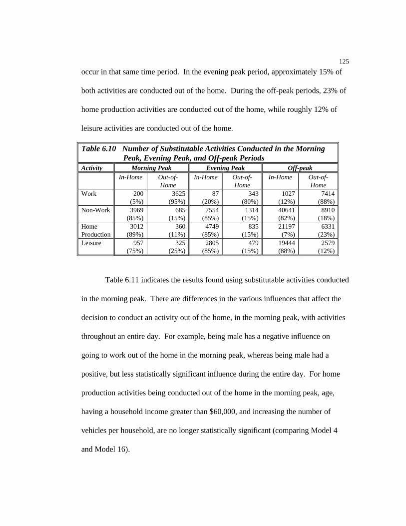
125
occur in that same time period. In the evening peak period, approximately 15% of
both activities are conducted out of the home. During the off-peak periods, 23% of
home production activities are conducted out of the home, while roughly 12% of
leisure activities are conducted out of the home.
Table 6.10 Number of Substitutable Activities Conducted in the MorningPeak, Evening Peak, and Off-peak Periods
Activity Morning Peak Evening Peak Off-peakIn-Home Out-of-
HomeIn-Home Out-of-
HomeIn-Home Out-of-
HomeWork 200
(5%)3625
(95%)87
(20%)343
(80%)1027
(12%)7414
(88%)Non-Work 3969
(85%)685
(15%)7554
(85%)1314
(15%)40641(82%)
8910(18%)
HomeProduction
3012(89%)
360(11%)
4749(85%)
835(15%)
21197(7%)
6331(23%)
Leisure 957(75%)
325(25%)
2805(85%)
479(15%)
19444(88%)
2579(12%)
Table 6.11 indicates the results found using substitutable activities conducted
in the morning peak. There are differences in the various influences that affect the
decision to conduct an activity out of the home, in the morning peak, with activities
throughout an entire day. For example, being male has a negative influence on
going to work out of the home in the morning peak, whereas being male had a
positive, but less statistically significant influence during the entire day. For home
production activities being conducted out of the home in the morning peak, age,
having a household income greater than $60,000, and increasing the number of
vehicles per household, are no longer statistically significant (comparing Model 4
and Model 16).

126
For leisure activities, household size and number of vehicles are no longer
statistically significant, while having a household income greater than $60,000 is still
significant, but to a lesser degree (comparing Model 5 to Model 17). It appears that
across all activities and those in the broad categories, the influence of various socio-
demographic characteristics is different for activities conducted in the morning peak
relative to those conducted over an entire day.
Table 6.11 Probability of Conducting a Substitutable Activity Out of theHome in the AM Peak
Variable Model 13 Model 14 Model 15 Model 16 Model 17all activities
AM Peakwork
AM Peaknon-workAM Peak
home productionAM Peak
leisureAM Peak
Constant -- ++ ++ -- *MALE ++ -- ++ ++ *AGE -- -- -- * --HHS -- * -- - *YRSR * + * * *EMPLYED ++ N/A ++ ++ *HHINC (> $60,000)
++ * * * +
VEC + * * * *
++ or - - indicates sign where p < .0001+ or - indicates sign where p < .01* no statistical significance
Table 6.12 reports the logit coefficients for substitutable activities conducted
in the morning peak. Looking across activity types in the morning peak, being a
male has a positive influence on conducting home production activities out of the
home. These findings suggest that the probability of conducting substitutable
activities in the morning peak is influenced by gender (being a male) and age. To
some extent, having an income greater than $60,000 and increasing the number of

127
vehicles in the household also influence the decision to conduct an activity out of the
home in the morning peak.
Table 6.12 Probability of Conducting a Substitutable Activity Out of theHome in the AM Peak (coefficients)
Variable Model 13 Model 14 Model 15 Model 16 Model 17all activities
AM Peakwork
AM Peaknon-workAM Peak
home productionAM Peak
leisureAM Peak
Constant -1.0093(-6.921)*
3.7096(11.241)
-1.2296(-5.147)
-2.0585(-6.166)
.037807(0.106)
MALE .21510(4.245)
-.71495(-4.478)
.44658(5.245)
.52960(4.601)
.13908(1.051)
AGE -.01020(-5.302)
-.01695(-3.343)
-.009398(-3.023)
-.002075(-0.485)
-.017695(-3.814)
HHS -.14560(-6.468)
.011806(0.181)
-.14652(-3.572)
-.16779(-2.937)
-.065803(-1.065)
YRSR -.03894(-1.871)
.17056(2.846)
-.023879(-0.702)
-.010232(-0.224)
-.066634(-1.243)
EMPLYED 2.3358(32.554)
-- .32146(3.228)
.62979(4.560)
-.070769(-.0456)
HHINC(> $60,000)
.29027(4.734)
.45653(2.519)
.30462(2.858)
.30196(2.111)
.44854(2.603)
VEH .08490(2.875)
-.18624(-2.314)
-.00085033(-0.017)
-.07106(-1.027)
.074223(1.018)
log likelihood -4708.703 -752.8865 -1894.182 -1105.271 -704.7023restricted loglikelihood
-5873.892 -776.0025 -1922.419 -1145.437 -725.8152
N 8476 3822 4654 3372 1282significancelevel
.00000 .00000 .00000 .00000 .00000
* z statistic (b/s.e.)
Household size has a negative influence on home production activities being
conducted out of the home in the morning peak, while is not statistically signficant
for leisure activities or work. Being a member of a higher income household does
not have a statistically significant influence on home production activities, but has a
positive influence on leisure activities being conducted out of the home in the

128
morning peak. Interestingly, years in the home (YRSR) has a positive influence on
working out of the home in the morning peak.
Using the submodel equivalence test (see Table 6.13), all substititutable
activities conducted in the morning peak should be separated into work and non-
work activities (Test 10). In addition, non-work activities should be treated
separately for home production and leisure activities in the morning peak (Test 11).
And, finally, testing the separate activities to all activities (Test 12) yields a
calculated χ2 that rejects the null hypothesis of no difference in the slope
coefficients.
Table 6.13 Submodel Equivalence Tests for Substitutable Activities (AM)Test Restricted
ModelLog Likelihood Unrestricted
ModelsLogLikelihood
Calculatedχχ2
Critical χχ2
10 Model 13 -4708.703 14 & 15 -2647.06 4123.26 21.9611 Model 15 -1894.182 16 & 17 -1809.97 168.41 21.9612 Model 13 -4708.703 16, 17, & 14 -2562.85 4291.69 34.27
Table 6.14 indicates the results for substitutable activities conducted in the
evening peak. Several of the factors that influence the decision to conduct a home
production activity out of the home in the evening peak differ from those over an
entire day. In this specification, household size and being employed influence this
decision in the evening peak, whereas being a male, age, having an income greater
than $60,000 and increasing the number of vehicles per household, influenced this
choice over an entire day (comparing Model 4 and Model 21).

129
In the evening peak, leisure activities conducted out of the home, are not
statistically significantly influenced by household size or number of vehicles. The
choice in the evening peak is influenced negatively by age and positively by being a
member of a household with an income greater than $60,000 (comparing Model 5
and Model 22).
Table 6.14 Probability of Conducting a Substitutable Activity Out of theHome in the PM Peak
Variable Model 18 Model 20 Model 21 Model 22all activities
PM Peaknon-work activities
PM Peakhome production
PM Peakleisure
PM PeakConstant -- -- -- -MALE ++ * * *AGE -- -- * --HHS -- -- -- *YRSR -- * * *EMPLYED ++ ++ ++ *HHINC (> $60,000)
++ ++ * ++
VEC ++ * * *
++ or - - indicates sign where p < .0001+ or - indicates sign where p < .01* no statistical significance
Table 6.15 reports the logit coefficients for substitutable activities conducted
in the evening peak. Previous studies indicate that activities are linked together
during peak hours through the process of trip chaining (Strathman and Dueker
1995; Strathman, Dueker and Davis 1993). The propensity to link activities before
and after work is thought to be due to increased time constraints within a household.
Bianco and Lawson (1996) found that females were more likely to be shopping and
picking up children in the evening peak. Thus, some of activities conducted in the

130
peak are substitutable activities, while others, such as shopping and picking up
children, require travel as a complement to the activity.
Table 6.15 Probability of Conducting a Substitutable Activity Out of theHome in the PM Peak (coefficients)
Variable Model 18 Model 19 Model 20 Model 21 Model 22all activities
PM Peakwork
PM Peaknon-workPM Peak
home productionPM Peak
leisurePM Peak
Constant -.9968(-6.675)*
1.9182(3.548)
-1.1107(-6.823)
-1.2620(-6.037)
-.73404(-2.794)
MALE .15780(2.844)
.18580(0.722)
.027814(.0456)
.13876(1.805)
-.16965(-1.670)
AGE -.01025(-4.988)
-.010536(-1.096)
-.0094494(-4.252)
-.0046068(-1.637)
-.019631(-5.303)
HHS -.16307(-6.277)
.23088(1.845)
-.16555(-5.737)
-.23735(-6.320)
-.035681(-0.776)
YRSR -.06855(-3.088)
-.12993(-1.311)
-.041745(-1.713)
-.010418(-0.332)
-.099948(-2.547)
EMPLYED .43212(6.021)
--- .23159(3.071)
.29911(3.207)
.098619(0.755)
HHINC(> $60,000)
.23764(3.489)
-.31719(-1.158)
.27231(3.626)
.12487(1.276)
.51138(4.281)
VEH .10353(3.277)
-.10239(-0.685)
.088202(2.545)
.058043(1.315)
.12630(2.196)
log likelihood -4247.459 -210.6903 -3666.726 -2320.728 -1312.615restricted loglikelihood
-4357.683 -216.5521 -3720.367 -2355.893 -1364.364
N 9298 430 8868 5584 3284significancelevel
.00000 .068426 .00000 .00000 .00000
* z statistic (b/s.e.)
In the case of substitutable activities, there appears to be a gender bias
towards men for all activities conducted in the evening peak (Model 18). However,
when the activities are separated, there is no longer a statistically significant
influence attributable to gender. The submodel equivalence tests for the
substitutable activities in the evening peak are reported in Table 6.16. The tests

131
indicate that the slope coefficients from the separated activities should be used as the
null hypothesis is rejected for tests 13, 14, and 15.
Table 6.16 Submodel Equivalence Tests for Substitutable Activities (PM)Test Restricted
ModelLogLikelihood
UnrestrictedModels
LogLikelihood
Calculatedχχ2
Critical χχ2
13 Model 18 -4247.45 19 & 20 -3877.45 739.99 21.9614 Model 20 -3666.726 21 & 22 -3633.34 66.76 21.9615 Model 18 -4247.45 21, 22, & 19 -3844.03 806.83 34.27
To test the effects of differences across time periods, it is necessary to
compare activities conducted out of the home across four periods of time: all day;
morning peak; evening peak; and off-peak. Table 6.17 indicates that there are
differences in magnitude and statistical significance, but not in direction (positive or
negative), from the various socio-demographic variables across the different periods
of the day. For example, employment (EMPLYED) has a positive influence, with
coefficients ranging from .43212, in the evening peak to 2.3358, in the morning
peak.
Being in a household in a higher income group has a positive influence on
conducting substitutable activities over an entire day, ranging from .12845, in off-
peak hours, to .29027, in the morning peak. The number of years an individual has
lived in a home has a negative, statistically significant, influence on conducting a
substitutable activity out of the home over an entire day and in the evening peak.
The activities disaggregated into time periods are tested in a submodel
equivalence test, -2[-43140.02 - ((-4708.703) + (-4247.459) + (-32664.16))] (Test

132
16). This yields a calculated χ2 of 3,039.396, rejecting the null hypothesis with 16
degrees of freedom and a critical χ2 at the 99.5% confidence level of 34.27. This
indicates that the slope coefficients for all substitutable activities should be separated
into morning, evening, and off-peak hours.
Table 6.17 Probability of Conducting an Activity Out of the Home forAll Substitutable Activities over Four Time Periods
Variable Model 1 Model 15 Model 18 Model 23all activities
all dayall activities
AM Peakall activities
PM Peakall activities
off-peakConstant -1.1612
(-25.207)*-1.0093(-6.921)
-.9968(-6.675)
-1.1433(-21.749)
MALE .16673(9.995)
.21510(4.245)
.15780(2.844)
.17671(9.186)
AGE -.00871(-13.724)
-.01020(-5.302)
-.01025(-4.988)
-.0091352(-12.496)
HHS -.12491(-16.421)
-.14560(-6.468)
-.16307(-6.277)
-.12678(-14.410)
YRSR -.02416(-3.546)
-.03894(-1.871)
-.06855(-3.088)
-.015264(-1.941)
EMPLYED 1.1396(49.250)
2.3358(32.554)
.43212(6.021)
1.0328(39.262)
HHINC (> $60,000)
.17319(8.533)
.29027(4.734)
.23764(3.489)
.12845(5.455)
VEH .07448(7.875)
.08490(2.875)
.10353(3.277)
.072484(6.682)
log likelihood -43140.02 -4708.703 -4247.459 -32664.16restricted loglikelihood
-45904.88 -5873.892 -4357.683 -34467.68
N 75766 8476 9298 57992significancelevel
.00000 .00000 .00000 .00000
* z statistic (b/s.e.)Table 6.18 reports the logit regression coefficients over four time periods for
work activities. Using the submodel equivalence test yields the following results: -
2[-4189.923 - ((-752.8865) + (-210.6903) + (-3105.973))], (Test 17), with a
calculated χ2 of 240.75. The null hypothesis is rejected with 16 degrees of freedom

133
and a critical χ2 at the 99.5% confidence level of 34.27. This indicates that work
activities should be separated into morning peak, evening peak, and off-peak hours.
Table 6.18 Probability of Conducting a Substitutable Work Activity Outof the Home for Over Four Time Periods
Variable Model 2 Model 14 Model 19 Model 24work
all daywork
AM Peakwork
PM Peakwork
off-peakConstant 2.7419
(20.710)*3.7096
(11.241)1.9182(3.548)
2.5650(16.860)
MALE -.13225(-2.206)
-.71495(-4.478)
.18580(0.722)
.024945(0.367)
AGE -.01336(-5.990)
-.01695(-3.343)
-.010536(-1.096)
-.013999(-5.33)
HHS .052311(1.962)
.011806(0.181)
.23088(1.845)
.035566(1.176)
YRSR .030668(1.273)
.17056(2.846)
-.12993(-1.311)
.018292(0.663)
EMPLYED -- -- --- ---HHINC (> $60,000)
.04966(0.731)
.45653(2.519)
-.31719(-1.158)
-.024505(-0.317)
VEH -.091411(-2.841)
-.18624(-2.314)
-.10239(-0.685)
-.74759(-2.053)
log likelihood -4189.923 -752.8865 -210.6903 -3105.973restricted loglikelihood
-4217.149 -776.0025 -216.5521 -3125.157
N 12693 3822 430 8441significance level .00000 .00000 .068426 .00000
* z statistic (b/s.e.)
The negative logit coefficient for (MALE) is only statistically significant in
the morning peak. Tenure in the home, (YRSR), is statistically significant for the
morning peak as well. The negative influence of increasing the number of vehicles
per household is no longer statistically significant when work is separated into peak
and off-peak periods.
Table 6.19 reports the results of non-work activities over four time periods.

134
Using the submodel equivalence test, -2[-28532.14 - ((-1894.182) + (-3666.726) +
(-22926.12))], (Test 18), yields a calculated χ2 of 90.224. The null hypothesis is
rejected with 16 degrees of freedom and a critical χ2 at the 99.5% confidence level
of 34.27, indicating that these activities should be separated with respect to time.
Table 6.19 Probability of Conducting a Substitutable Non-work ActivityOut of the Home for Over Four Time Periods
Variable Model 3 Model 15 Model 20 Model 25non-workall day
non-workAM peak
non-workPM Peak
non-workoff-peak
Constant -1.0480(-18.383)*
-1.2296(-5.147)
-1.1107(-6.823)
-1.0285(-16.319)
MALE .11196(5.200)
.44658(5.245)
.027814(.0456)
.096418(4.029)
AGE -.009986(-12.638)
-.009398(-3.023)
-.0094494(-4.252)
-.010038(-11.416)
HHS -16066(-15.726)
-.14652(-3.572)
-.16555(-5.737)
-.015988(-14.086)
YRSR -.02578(-2.964)
-.023879(-0.702)
-.041745(-1.713)
-.022683(-2.341)
EMPLYED .33409(12.693)
.32146(3.228)
.23159(3.071)
.35128(11.963)
HHINC (> $60,000)
.17258(6.445)
.30462(2.858)
.27231(3.626)
.14613(4.907)
VEH .084754(6.976)
-.00085033(-0.017)
.088202(2.545)
.090371(6.720)
log likelihood -28532.14 -1894.182 -3666.726 -22926.12restricted loglikelihood
-29048.03 -1922.419 -3720.367 -23344.09
N 63073 4654 8868 49551significance level .00000 .00000 .00000 .00000
* z statistic (b/s.e.)
Being a male is not statistically significant for non-work activities in the
evening peak. However, during the morning peak and off-peak hours, being a male
has a postive influence on conducting substitutable non-work activities out of the
home. Increasing the number of vehicles per household has a positive effect on

135
conducting substitutable non-work in the off-peak hours, but is not statistically
significant in either the morning or the evening peaks.
Table 6.20 Probability of Conducting a Substitutable Home ProductionActivity Out of the Home over Four Time Periods
Variable Model 3 Model 16 Model 21 Model 26home
productionall day
homeproductionAM Peak
homeproductionPM Peak
homeproduction
off-peakConstant -.88031
(-12.221)*-2.0585(-6.166)
-1.2620(-6.037)
-.75424(-9.520)
MALE .18774(7.044)
.52960(4.601)
.13876(1.805)
.15858(5.369)
AGE -.008177(-8.248)
-.002075(-0.485)
-.0046068(-1.637)
-.0085867(-7.827)
HHS -.21888(-17.103)
-.16779(-2.937)
-.23735(-6.320)
-.21294(-15.110)
YRSR -.025896(-2.399)
-.010232(-0.224)
-.010418(-0.332)
-.024870(-2.081)
EMPLYED .52482(16.019)
.62979(4.560)
.29911(3.207)
.53750(14.764)
HHINC (> $60,000)
.17269(5.222)
.30196(2.111)
.12487(1.276)
.17092(4.679)
VEH .063527(4.215)
-.07106(-1.027)
.058043(1.315)
.068148(4.113)
log likelihood -18050.32 -1105.271 -2320.728 -14420.51restricted loglikelihood
-18569.96 -1145.437 -2355.893 -14844.67
N 36484 3372 5584 27528significance level .00000 .00000 .00000 .00000
* z statistic (b/s.e.)
Table 6.20 indicates that the socio-demographic influences on the probability
of conducting a substitutable home production activities vary across the four time
periods. For example, the positive influence of being a male is not statistically
significant in the evening peak, however, it is in the morning peak and during the
off-peak hours of the day. Neither being in a higher income household nor

136
increasing the number of vehicles per household have a statistically significant
influence in either peak period.
The submodel equivalence test (Test 19) is: -2[-18050.32 - ((-1105.271) +
(-2320.728) + (-14420.51))]. This yields a calculated χ2 of 90.224, rejecting the
null hypothesis with 16 degrees of freedom and a critical χ2 at the 99.5% confidence
level of 34.27. This indicates that substitutable home production activities should be
separated into separate time periods.
Table 6.21 illustrates that substitutable leisure activities appear to be less
variable over the four time periods. Being a male and being employed remain
statistically insignificant, while age maintains a negative influence. Being in a higher
income household has a positive influence, with differences in magnitude on the
probability of conducting a substitutable leisure activity out of the home.
The submodel equivalence test for these models (Test 20) is constructed as
follows: -2[-9998.846 - ((-704.7023) + (-1312.615) + (-7859.820))]. This yields a
calculated χ2 of 243.417, rejecting the null hypothesis with 16 degrees of freedom
and a critical χ2 at the 99.5% confidence level of 34.27. This indicates that
substitutable leisure activities should be disaggregated into time periods as well.
Across all four periods of time, there is no statistically significant influences
attributed to gender for substitutable leisure activities. Conducting leisure activities
out of the home is negatively influenced by household size in the off-peak hours,
while the influence is not statistically significant during either the morning or

137
evening peaks. Being employed is not a statistically significant influence during any
of the time periods. Increasing the number of the vehicles in the household appears
to not have a statistically significant influence on conducting leisure activities out of
the home in either the morning or evening peaks.
Table 6.21 Probability of Conducting a Substitutable Leisure ActivityOut of the Home Over Four Time Periods
Variable Model 4 Model 17 Model 22 Model 27leisureall day
leisureAM Peak
leisurePM Peak
leisureoff-peak
Constant -1.1615(-12.169)*
.037807(0.106)
-.73404(-2.794)
-1.2897(-11.912)
MALE .059747(1.593)
.13908(1.051)
-.16965(-1.670)
.08374(1.961)
AGE -.014786(-10.983)
-.017695(-3.814)
-.019631(-5.303)
-.014558(-9.460)
HHS -.074025(-4.266)
-.065803(-1.065)
-.035681(-0.776)
-.081524(-4.114)
YRSR -.033772(-2.245)
-.066634(-1.243)
-.099948(-2.547)
-.024663(-1.430)
EMPLYED -.030957(-0.691)
-.070769(-.0456)
.098619(0.755)
-.01937(-0.381)
HHINC(> $60,000)
.17875(3.821)
.44854(2.603)
.51138(4.281)
.094381(1.749)
VEH .10923(5.195)
.074223(1.018)
.12630(2.196)
.10998(4.598)
log likelihood -9998.846 -704.7023 -1312.615 -7859.820restricted loglikelihood
-10132.88 -725.8152 -1364.364 -7952.872
N 26589 1282 3284 22023significance level .00000 .00000 .00000 .00000
* z statistic (b/s.e.)
The findings indicate that it is important to recognize the significance of the
peak behaviors over the course of a day. To incorporate this notion, Table 6.22,
presents three new time-specific variables. Approximately the same percentage of
substitutable activities are conducted during the morning and the evening peaks
(between 11% and 12%).

138
Table 6.22 Time VariablesVariable Mean Std. Dev. DefinitionPEAK .2346 .4237 Both AM (7:00 to 9:00) & PM (4:00 to 6:00) peaksAM PEAK .1119 .3152 7:00 to 9:00 AMPM PEAK .1227 .3281 4:00 to 6:00 PM
The general model is respecified to include “peak” as a variable:
(6.6) log(P/1-P) = f(MALE, AGE, HHS, YRSR, EMPLYD, HHINC, VEH,PEAK)
The logit coefficients for substitutable activities over an entire day are reported in
Table 6.23. Model 28 indicates that “peak” has a positive influence on the decision
to conduct a substitutable activity out of the home.
Crown (1998) suggests testing the contribution of new variables. In this
test, a χ2 is calculated, using the log of the maximum likelihoods for the unrestricted
model and the restricted model. The number of variables dropped in the restricted
model determines the degrees of freedom. If the calculated χ2 statistic is greater
than the critical χ2 at the 99.5% confidence level, then the null hypothesis that the
slope coefficients of the tested variable is jointly equal to zero is rejected. Test 21,
in Table 6.25, indicates that adding “PEAK” rejects the null hypothesis.
Table 6.23 Probability of Conducting a Substitutable Activity Out of theHome
Variable Model 28all activities
all dayConstant -1.2125
(26.191)*MALE .17065
(10.215)

139
AGE -.0089072(-14.007)
HHS -.12617(-16.560)
YRSR -.024432(-3.580)
EMPLYED 1.1369(49.075)
HHINC (> $60,000) .17223(8.471)
VEH .074075(7.819)
PEAK .27023(14.159)
log likelihood -43040.98restricted log likelihood -45904.88N 75766significance level .00000
* z statistic (b/s.e.)
It should be noted that previous models indicated that there are differences
in the morning peak and in the evening peak with respect to influences of socio-
demographic characteristics and activity choices. Therefore, a new model is
specified to test the influence of each peak separately on the decision to conduct a
substitutable activity out of the home. The model was specified as follows:
(6.7) log(P/1-P) = f(MALE, AGE, HHS, YRSR, EMPLYD, HHINC, VEH, AMPEAK, PM PEAK); conditioned on activity type
Table 6.24 indicates the results when the peaks are disaggregated into the
morning and evening peaks. There are several differences across activities with
respect to the influence of two peak periods. For all substitutable activities, the
morning peak has a positive influence and the evening peak has a negative influence
on the probability of conducting a substitutable activity out of the home.
Table 6.24 Probability of Conducting Substitutable Activities Out of the
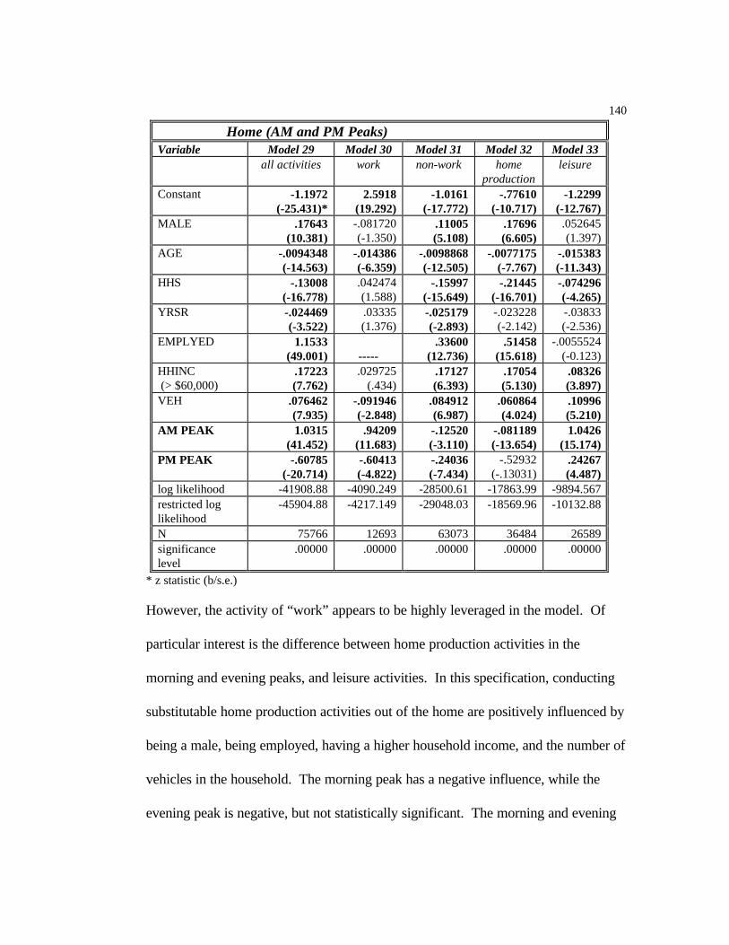
140
Home (AM and PM Peaks)Variable Model 29 Model 30 Model 31 Model 32 Model 33
all activities work non-work homeproduction
leisure
Constant -1.1972(-25.431)*
2.5918(19.292)
-1.0161(-17.772)
-.77610(-10.717)
-1.2299(-12.767)
MALE .17643(10.381)
-.081720(-1.350)
.11005(5.108)
.17696(6.605)
.052645(1.397)
AGE -.0094348(-14.563)
-.014386(-6.359)
-.0098868(-12.505)
-.0077175(-7.767)
-.015383(-11.343)
HHS -.13008(-16.778)
.042474(1.588)
-.15997(-15.649)
-.21445(-16.701)
-.074296(-4.265)
YRSR -.024469(-3.522)
.03335(1.376)
-.025179(-2.893)
-.023228(-2.142)
-.03833(-2.536)
EMPLYED 1.1533(49.001) -----
.33600(12.736)
.51458(15.618)
-.0055524(-0.123)
HHINC (> $60,000)
.17223(7.762)
.029725(.434)
.17127(6.393)
.17054(5.130)
.08326(3.897)
VEH .076462(7.935)
-.091946(-2.848)
.084912(6.987)
.060864(4.024)
.10996(5.210)
AM PEAK 1.0315(41.452)
.94209(11.683)
-.12520(-3.110)
-.081189(-13.654)
1.0426(15.174)
PM PEAK -.60785(-20.714)
-.60413(-4.822)
-.24036(-7.434)
-.52932(-.13031)
.24267(4.487)
log likelihood -41908.88 -4090.249 -28500.61 -17863.99 -9894.567restricted loglikelihood
-45904.88 -4217.149 -29048.03 -18569.96 -10132.88
N 75766 12693 63073 36484 26589significancelevel
.00000 .00000 .00000 .00000 .00000
* z statistic (b/s.e.)
However, the activity of “work” appears to be highly leveraged in the model. Of
particular interest is the difference between home production activities in the
morning and evening peaks, and leisure activities. In this specification, conducting
substitutable home production activities out of the home are positively influenced by
being a male, being employed, having a higher household income, and the number of
vehicles in the household. The morning peak has a negative influence, while the
evening peak is negative, but not statistically significant. The morning and evening

141
peaks have a strong positive influence on the probability of conducting substitutable
leisure activity out of the home.
Table 6.25 reports the results of a set of tests to determine the contribution
of the new variables and submodels. In each case, the calculated χ2 is greater than
the critical χ2 at the 99.5% confidence level, rejecting the null hypothesis that the
slope coefficients of the tested variables are jointly equal to zero.
Table 6.25 Tests for the Contribution of New Variables and SubmodelEquivalence Tests
Test RestrictedModel
LogLikelihood
UnrestrictedModels
LogLikelihood
Calculatedχχ2
Critical χχ2
21 Model 1 -43140.02 28 -43040.98 198.08 7.8922 Model 28 -43040.98 29 -41908.88 2264.20 7.8923 Model 1 -43140.02 29 -41908.88 2462.28 10.6024 Model 2 -4189.923 30 -4090.249 199.34 10.6025 Model 3 -28532.14 31 -28500.61 63.06 10.6026 Model 4 -18050.32 32 -17863.99 372.66 10.6027 Model 5 -9998.846 33 -9894.567 208.56 10.6028 Model 29 -41908.88 30 & 31 -32590.859 18636.04 21.9629 Model 31 -28500.61 32 & 33 -27758.557 1484.106 21.9630 Model 29 -41908.88 30, 32 & 33 -31848.806 20119.988 34.27
Disaggregating the peak periods into smaller time intervals may also increase
the understanding of travel behaviors. For example, if an out-of-home activity
occurs within the first five minutes of the morning peak, then it can be assumed that
the activity occurred just after leaving home (residential pre-commute activity).
However, if the activity occurs near the workplace (employment post-commute
activity), or somewhere in the middle, it may be possible to test some of the urban
design issues revolving around the preconceived notions about how people will
change their travel patterns if appropriate land uses are adopted.

142
It may also be important to further disaggregate off-peak hours to capture the level
of activity being conducted during the mid-day. For example, trips being generated
during the noon hour may be influencing the logit regression coefficients.
6.3.3 Socio-demographic Models
The next set of models examines differences across all activities by age
groups, specific household sizes, employment status, and income groups. Table
6.26 lists the variables that are included in the specification of the models.
Table 6.26 Socio-demographic VariablesVariable Mean Std. Dev. DefinitionMID .7009 .4579 18 - 55 years of ageH1 .1172 .3818 Single person householdH2 .4299 .4951 Two person householdH4 .2277 .4194 Greater than 3 person householdLOWIN (<$25,000) .0079 .0886 Household income less than $25,000FEM .5064 .5000 Full-time employmentPEM .0923 .2894 Part-time employmentRET .1926 .3944 RetiredHM .0687 .2530 Homemaker
Age is limited to the years (18 through 55) during which a person is most
likely to be working (MID). Household size is classified as (H1) for a single
individual, (H2) for a couple, and (H4) with greater than three members, to
represent households with children. Three-person households are the omitted
variable. Household income is categorized as lower if it is below $25,000
(LOWIN). Middle income households are the omitted variable. It should be noted
that the income data collected for this dissertation is somewhat troublesome. The
original survey categories were not representative of the local total household
income distribution. As a result, more work may be needed to extract meaningful

143
information from this data set. Employment status is divided into full (FEM) and
part time (PEM) work. Non-working status is represented by retirement (RET) and
homemaker (HM). Unemployed individuals are the omitted variable.
Table 6.27 indicates the results of the various combinations of socio-
demographic variables. Due to programming constraints, the entire set of variables
could not be run in a single model specification. The model is specified as follows:
(6.8) log(P/1-P) = f(MALE, MID, HHS, FEM, PEM, RET, HM,LOWIN, HIINC, VEH, AM PEAK, PM PEAK, YRSR);
There are no direct comparative tests for Models 34, 35, 36, or 37, as the
specifications are different in order to add dummy variables that will allow for the
calculation of odds ratios. Crown (1998) explains that odds ratios represent the
ratio of the probabilities of the outcome occurring for sample members with a value
of one for the dummy versus those in a reference group. Odds ratios will be used as
an application for the models in Chapter Seven. Crown (1998) also points out that
odds ratios provide only information on the relative odds of the event occurring (in
this case, the event is conducting a substitutable activity out of the home) for the
two categories of the dummy variable. Odds ratios are not calculated for each case.
It is also not possible to examine how the odds ratio might vary for subgroups with
the sample. However, it provides insight into the effect of the variables in the
models.

144
As indicated in previous models, it may be important to also look at
difference across activity types. However, this dissertation will look at the addition
of socio-demographic variables over all substitutable activities, all day, only. As
expected, full time employment and part time employment have a positive influence
on the decision to conduct a substitutable activity out of the home. Being retired or
being a home maker has a negative impact on this decision. Unemployed individuals
are the omitted category. Being a household with a lower income has a negative
influence on conducting substitutable activities out of the home, although it appears
to be statistically insignificant. Being between the age of 18 and 55 years has a
strong, positive influence on conducting subsitutable activties out of the home.

145
Table 6.27 Probability of Conducting a Substitutable Activity Out of theHome (Employment Status and Income Levels)
Variable Model 34 Model 35 Model 36all activities all activities all activities
Constant -1.8347(-45.299)*
-1.8247(-66.327)
-1.4763(-41.326)
MALE .18043(10.604)
.17364(9.938)
.20925(12.167)
MID .37427(14.848)
.54005(22.732)
.28275(10.591)
HHS -.13151(-16.969)
-.12404(-15.808)
-.13795(-17.751)
YRSR -.034948(-5.238)
EMPLYED 1.1170(45.762)
FEM .89234(38.714)
.80319(34.802)
PEM .59477(17.845)
.49443(14.799)
RET -.61853(-16.000)
HM -.37220(-7.897)
LOWIN < $25,000 -.29591(-2.668)
-.28470(-2.592)
-.25990(-2.356)
HIINC > $60,000 .13224(6.369)
.13712(6.569)
.12597(6.053)
VEH .076102(7.897)
.076555(8.152)
.071802(7.656)
AM PEAK 1.0280(41.311)
1.0222(41.183)
1.0285(41.317)
PM PEAK -.60987(-20.779)
-.61669(-20.989)
-.61550(-20.948)
log likelihood -41901.71 -41988.63 -41892.19restricted log likelihood -45904.88 -45904.88 -45904.88N 75766 75766 75766p value .00000 .00000 .00000
* z statistic (b/s.e.)

146
The following model includes household size:
(6.9) log(P/1-P) = f(MALE, MID, H1, H2, H4, EMPLYED, LOWIN, HIINC,VEH, AM PEAK, PM PEAK, YRSR);
Table 6.28 Probability of Conducting a Substitutable Activity Out of theHome (Household Size)
Variable Model 37all activities
Constant -2.3633(-48.784)*
MALE .17878(10.501)
MID .38775(15.219)
H1 .43143(13.662)
H2 .21805(8.735)
H4 -.099827(-3.709)
EMPLYED 1.1165(45.704)
LOWIN -.30207(-2.720)
HIINC .14693(7.026)
VEH .09126(9.111)
AM 1.0309(41.410)
PM -.61034(-20.785)
YRSHOME -.0334457(-5.012)
log likelihood -41873.12restricted log likelihood -45904.88N 75766p value .00000
* z statistic (b/s.e.)
Table 6.28 indicates that single-person households and two-person
households have a positive influence on the decision to conduct a substitutable

147
activity out of the home. However, being in a household with more than three
persons (proxy for children) has a negative influence on the decision to conduct a
substitutable activity out of the home, relative to the omitted category, three-person
households. Being in a lower income household also has a negative influence in this
specification relative to the omitted category, middle income.
6.4 SUMMARY
Based on logit regression coefficients, the decision to participate in a
“substitutable” activity out of the home, is influenced on the activity type itself, the
socio-demographics of the individuals participating in the activity, and their living
arrangement. The submodel equivalence tests suggest that traditional travel
forecasting models using aggregate data may be missing information found in the
disaggregate activity data. Currently, much of the information contained in activity
data is lost through ad hoc reaggregation or the use of traditional assumptions about
behaviors.
The data for this dissertation is unique in the fact that it contained detailed
information on activities conducted in the home. The use of this level of detail has
contributed towards an understanding of factors that affect household-level
travel/activity decisions. A set of models are presented that illustrate the influences
of the socio-demographic variables previously associated with travel behaviors. The
data is sorted into discrete activity types and tested to determine what, if any,

148
additional information, with respect the slope of the logit regression coefficients, is
gained. The data is also sorted by time of day to determine additional slope
coefficient differences. For example, by sorting the data by time of day, it was
possible to look at the effect of various socio-demographic variables on the
travel/activity choices of individuals. It is important to note that it was necessary to
include morning, evening, and off-peak hours in the model to fully understand the
influence time of day. The models are extended to include variables for the morning
and evening peaks, across the major activity types. It is clear that across different
activities types, the influence of the time of day differs.
This dissertation found that one- and two-person households had a positive
propensity to conduct substitutable activities out of the home. This finding has
implications for travel forecasting. Pisarski (1996) found that there has been an
increase in the share of non-family households, made up of persons living alone or in
multiperson, nonfamily, living arrangements. Data that uses the household as the
unit of analysis is vulnerable to error if the household structure within the unit is not
understood. In other words, a household with four family members will function
differently from a household made up of four individual adults, living independently
of each other. Further research is needed to understand the differences in travel
decisions for various household types (including households with two earners,
multiperson, non-family households, and single person households). This also

149
confirms the importance of a better understanding of the role of participation
parameters for household members.
The probability of conducting a substitutable activity out of the home is
strongly influenced by employment. For this reason, it may be important to examine
the impact of the number of wage earners and their relative contribution to the total
household income.
The basic decision to use transport in the production of various activities has
been examined for a specific set of substitutable activities that can be conducted
either in or out of the home. An extension of this methodology could be used to
understand the socio-demographic and time dynamics of other activities that require
travel.

150
CHAPTER SEVEN
APPLICATIONS
7.1 INTRODUCTION
Logit coefficients offer an opportunity to understand the influence of specific
factors on the decision to conduct a substitutable activity out of the home. For
travel forecasting purposes, it is important to understand the probability of an
activity being conducted out of the home, indicating the use of transport as an input.
The applications presented include the use of the logit coefficients to calculate odds
ratios and to determine the probability of an activity being conducted out of the
home, for different activity types, times of day, and socio-demographic
characteristics is a set of representative case studies.
7.2 ODDS RATIOS
The logit coefficient interpretations are able to indicate positive or negative
influences for various factors. To measure the effect of dummy variables on the
probability of an event, odds ratios are calculated (Crown 1998):
(7.1) odds ratiok = ebk

151
Table 7.1 reports the calculated odds ratios for Models 29, 30, 32, and 33.
The odds ratios are calculated for statistically significant coefficients only. The
results indicated that men have a probability that is 19% higher than women of
conducting a substitutable activities out of the home. However, this probability is
reduced to 12% for work. While employed individuals have a probability that is
more than three times higher than non-employed persons, they have are only 1.67
times higher probability of conducting home production activities out of the home.
Of particular interest is that the probability of conducting an out-of-home
leisure activity is 2.83 times higher in the morning peak and 1.27 times higher in the
evening peak, than at other times. This has implications for policies that try to
encourage the use of transit or carpooling for commuting options. Such options are
likely to reduce the opportunities to participate in these leisure activities. The
decision to change modes in order to participate in a Transportation Demand
Management (TDM) program would include this “opportunity cost” of time use.
Table 7.1 Odds Ratios of Conducting a Substitutable Activity Out of theHome
Variable Model 29 Model 30 Model 32 Model 33all activities work home
productionleisure
MALE 1.19 1.12 1.19 *EMPLYED 3.16 N/A 1.67 *HIINC (> $60,000) 1.18 * 1.18 1.09AM PEAK 2.80 2.57 .92 2.83PM PEAK .54 .54 * 1.27
* not statisically significant (p >.05)

152
Table 7.2 reports the calculated odds ratios for the statistically signficiant
dummy variables in Models 34, 35, 36, and 37.
Table 7.2 Odds Ratios of Conducting a Substitutable Activity Out of theHome (Employment Status and Household Size)
Variable Model 34 Model 35 Model 36 Model 37all activities
all dayall activities
all dayall activities
all dayall activities
all dayMALE 1.20 1.19 1.23 1.19MID 1.45 1.72 1.32 1.47H1 1.54H2 1.24H4 .90EMPLYED 3.06 -- -- 3.05FEM -- 2.44 2.23 --PEM -- 1.81 1.64 --RET -- -- .53 --HW -- .68 -- --HIINC (> $60,000) 1.14 1.15 1.13 1.16AM PEAK 2.80 2.78 2.79 2.80PM PEAK .54 .54 .54 .54
The odds ratios indicate that the probability of a man conducting a
substitutable activity out of the home is approximately 1.20 times higher than a
woman, holding everything else constant. The variable (MID) represents being
between 18 and 54 years of age. The varying odds ratios may indicate that the
dummy variable represents too varied a subgroup.
Individuals in a single person household have the highest probability of
conducting a substitutable activity out of the home, (1.54 times higher than
individuals living in larger households). Persons in households with more than three
persons have a probability that is .90 times that of individuals in three households.
Employed persons have a probability 3.06 times higher than unemployed persons of

153
conducting substitutable activities out of the home. Persons who are employed full-
time have a probability that is approximately 2.3 times higher than others, while
part-time workers have a probability that is approximately 1.7 times higher than
unemployed individuals. Retirees have a probability that is .68 times, while
homemaker have a probability .53 times that of unemployed individuals of
conducting a substitutable activity out of the home. Individuals from a household
with greater than $60,000 income have a probability that is 1.14 times higher than
individuals in middle income households.
7.3 REPRESENTATIVE CASES
Crown (1998) points out that it is often useful to present the probabilities for
particular cases with characteristics of interest. Using the estimated coefficients,
various representative values for the explanatory variables can be applied and the
associated probabilities calculated. This application provides information on the
probability of an activity being conducted out of the home for a specific combination
of the characteristics in the model. It also allows a range of predicted probabilities
to be generated using a set of values for the explanatory variables similar to a series
of case studies. A specific set of factors are varied, holding the remaining factors
constant. With this formation, it is possible to determine differences in probabilities
for various groups of individuals with shared characteristics.

154
A representative case model can illustrate the impact on the probability of
conducting a substitutable activity out of the home, given an income constraint. In
addition, employment status provides a proxy for restrictions on time. These
factors, in combination with household size, are reported in Table 7.3. This table
indicates the probability of conducting substitutable activities out of the home from
each case. All of the logit regression coefficients per model are incorporated.
Table 7.3 Probability of Conducting a Substitutable Activity Out of the Homeby Employment Status, Household Size, and Income Group
EmploymentStatus
Household Size Low Income Middle Income High Income
Full-time 1 34% 40% 44%Full-time 4 26% 31% 34%Part-time 1 28% 33% 37%Part-time 4 20% 25% 27%Retiree 2 10% 13% 14%Retiree 4 8% 10% 11%
It is clear that individuals from very different household types have similar
probability patterns. This reinforces the need to understand the underlying utility
functions. For example, consider trying to predict a change in travel behavior for an
individual from a low-income, one-person household, who works full-time; an
individual from a high-income, four-person household who works full time; and an
individual from a middle income, one-person household who works part-time. They
all have approximately the same probability with respect to conducting a
substitutable activity out of the home (34%, 34%, and 33%, respectively).

155
Figure 7.1 indicates graphically these relationships. A high-income
individual from a household of four has approximately the same probability of
conducting a substitutable activity out of the home as an individual from a single-
person, lower income household, while facing a different set of constraints. For
example, the low-income individual may be influenced by a shortage of time due to a
full-time job and the lack of accessibility to a “substitute” on route to or from work.
0%
5%
10%
15%
20%
25%
30%
35%
40%
45%
Full-time/HH of 1
Full-time/HH of 4
Part-time/HH of 1
Part-time/HH of 4
Retiree/HH of 2
Retiree/HH of 4
Low IncomeMiddle IncomeHigh Income
Figure 7.1 Probability of Conducting a Substitutable Activity Out of the Homeby Employment Status, Household Size, and Income Group

156
The representative case model in Table 7.4, the Probability of Conducting a
Substitutable Home Production Activity Out of the Home by Gender and Household
Size, is based on the following sample values: an individual living in a two-person
household; who is employed with a total household income greater than $60,000;
living in the same residents for three years; and having two vehicles for the
household.
There are notable differences across the various time periods. Men have a
greater probability than women of conducting a substitutable home production
activity out of the home. However, this differences appears to be less during the
evening peak.
Table 7.4 Probability of Conducting a Substitutable Home ProductionActivities Out of the Home by Gender and Household Size
All Day Morning Peak Evening PeakHousehold Size Male Female Male Female Male FemaleOne-Person 37% 24% 16% 10% 21% 19%Two-Person 23% 20% 14% 9% 18% 16%Three-Person 20% 17% 12% 8% 14% 13%
Figure 7.2 indicates graphically the gender differences in the probability of
conducting a substitutable home production activity, by household size, and gender,
over an entire day. One of the most significant differences in activity location choice
(in or out of the home) is between one- and two-person households with respect to
gender. Single men have a greater probability of conducting home production
activities out of the home. However, when men live in two-person households, this
probability is greatly reduced. Gronau’s (1977) comments on the possibility of the

157
marginal productivity of work at home (house work) falling below the real wage,
resulting in no home production activity, may explain the greater probability of men
making the decision to conduct home production activities out of the home. Evans’
(1972) discussion related to doing housework to save money, may indicate that men
in single-person households would rather save time than money. It is also possible
that single men have a different set of preferences for home environmental or social
factors.
0%
5%
10%
15%
20%
25%
30%
35%
40%
HH of 1 HH of 2 HH of 3
MaleFemale
Figure 7.2 Probability of Conducting a Substitutable Home Production ActivityOut of the Home by Household Size and Gender
Women in three-person households have the lowest probability of
conducting home production activities out of the home. This may reinforce the
notions of productivity at home production activities with respect to household

158
structure. As previously noted, if household size is a proxy for children, although
this analysis did not include the ages of the children, it may indicate that women may
have a higher degree of productivity for these activities in the home. Again, the
theoretical set of income, time, distance, and participation constraints would suggest
this outcome.
Further research may be necessary to determine the effect of the employment
status of other members of the household. In other words, if there is a homemaker
in the household, is the probability of conducting a home production activity out of
the home reduced for the worker. This would also relate to the notions of
comparative advantage and specialization within the context of a utility
maximization framework.
There is an interest in understanding the specific influence children play in
travel patterns. It may be equally important to include household dissolutions that
result in children being an intermittant member of the households of either parent.
According to Wineberg and McCarthy (1993), approximately five million, or
roughly 10% of all currently married couples in the United States have experienced
some form of separation and reconciliation. During this period, the couples were
continually moving between a state of separation and reconciliation.
Further research is needed to determine the effects on travel from the
“churning” of household structure. Men in single-person households have the
highest probability of conducting home production activities out of the home and

159
separation generally results in men forming a single-person household. If one of the
members of the household relocates, the underlying household production function
is changed and the entire set of household activities may be affected. This is also the
case for separated or divorced households who share custody of their children. The
travel patterns of the household would change depending on the makeup of the
household, at any given time. This dissertation indicates that household size does
affect decisions to conduct an activity in or out of the home.
0%
5%
10%
15%
20%
25%
All Day AM Peak PM Peak
MaleFemale
Figure 7.3 Probability of Conducting a Home Production Activity Out of the Homeby Time of Day and Gender
Figure 7.3 indicates differences in the probability of conducting a home
production activity out of the home by gender and time of day. Although men have
a greater probability than women of conducting these activities out of the home over

160
an entire day, there is a greater difference in the morning peak. This representative
case is based on a two-person household (see Table 7.4).
Age has been determined as an important indicator of mobility. Table 7.5
indicates increasing age impacts on the decision to conduct a substitutable home
production activity out of the home. For example, 28 year old men have 4% greater
probability of conducting a substitutable home production activity out of the home
than 35 year olds. This difference increases to 22% with respect to a 67 year olds,
over the entire day. Across age groups, the probability for men is approximately
14% greater over the entire day, 37% greater in the morning peak, and 11% greater
in the evening peak, compared to women, of conducting a substitutable home
production activities out of the home.
Table 7.5 Probability of Conducting a Substitutable Home ProductionActivity Out of the Home by Gender and Age
All Day Morning Peak Evening PeakMale Female Male Female Male Female
28 Years Old 24% 21% 14% 9% 18% 16%35 Years Old 23% 20% 14% 9% 18% 16%67 Years Old 19% 16% 13% 8% 16% 14%
It may be unwise to make too much of these differences with respect to
forecasting the behavior of older men and women in the future, however. There
may be a cohort effect that applies to individuals who are currently in these older
age groups. The mobility behaviors of today’s 40 year olds may continue as they
age, as a group norm. As a result, it will be necessary to track the mobility of each
cohort over time. This is especially important as the “baby boom” cohort enters

161
retirement age. If their rates of mobility continue to be high, then forecasts of
declines in congestion may be exaggerated. However, if they are not commuting to
work in the peak, their travel behaviors may cause different patterns of peaks.
Activity choice was a concern in the “new home economics” literature, due
to the possible inability to differentiate leisure from home production activities for
women. However, gender (MALE) was not a statistically significant variable in the
context of the choice to conduct a leisure activity in or out of the home. The
decision to participate in a leisure activity may still represent a problem. However,
once leisure has been chosen as the desired activity, the location of that activity
appears not to be influenced by gender.
Table 7.6 Probability of Conducting a Substitutable Activity Out of the Homeby Activity Type and Household Size
All Day Morning Peak Evening PeakHouseholdSize
HomeProduction
Leisure HomeProduction
Leisure HomeProduction
Leisure
One-Person 37% 20% 16% 47% 21% 24%Two-Person 23% 19% 14% 46% 16% 23%Three-Person 20% 18% 12% 44% 14% 23%
Table 7.6 indicates the differences in the probability of conducting a
substitutable activity out of the home by time of day and household size. There are
differences in the location choice for leisure activities during the peaks. Individuals
in single-person households have a 47% probability of conducting their morning
peak leisure activities out of the home. In terms of household size and activity
choice, leisure activities conducted out of the home are fairly stable across

162
household size, whereas home production activities differ between one and two
person households more than between two- and three-person households. This
would be an indication of the effect of an additional person (children) impacts home
production location decisions more than leisure activities. Different participation
patterns of household members are also reflected in this findings.
As Table 7.7 indicates, the probability of conducting home production or
leisure activities out of the home declines with age. There is a reduction in leisure
and home production activities being conducted out of the home by 35 year old
individuals compared to 28 year olds. This decline continues at a greater rate for
leisure than home production activities by the time an individual reaches 67 years of
age.
Table 7.7 Probability of Conducting a Substitutable Activity Out of the Homeby Activity Type and Age
All Day Morning Peak Evening PeakAge Home
ProductionLeisure Home
ProductionLeisure Home
ProductionLeisure
28 Years 24% 20% 14% 49% 18% 26%35 Years 23% 19% 14% 46% 18% 23%67 Years 19% 13% 13% 32% 16% 14%
The differences across the times of day by age group continues to show
declines in mobility. The probability of conducting substitutable leisure activities out
of the home decline more rapidly with increasing age than home production
activities. Figure 7.4 illustrates the differences over an entire day.

163
0%
5%
10%
15%
20%
25%
28 Years Old 35 Years Old 67 Years Old
Home ProductionLeisure
Figure 7.4 Probability of Conducting a Substitutable Activity Out of theHome by Activity Type and Age
The number of vehicles available to household members appears to increase
the probability of conducting a substitutable activity out of the home. However, it
must be recognized that the desire to use transport within the context of the
household production function may have a strong influence on the purchase of
additional vehicles.
As indicated in Table 7.8, households without vehicles actually have a higher
probability of conducting substitutable home production activities out of the home in
the morning peak than other households. There does not appear to be a strong
influence on the probability of conducting substitutable home production activities
out of the home from owning a third vehicle.
Table 7.8 Probability of Conducting a Substitutable Home Production

164
Activity Out of the Home by Number of Vehicles and GenderAll Day Morning Peak Evening Peak
Number ofvehicles
Male Female Male Female Male Female
None 21% 18% 16% 10% 16% 14%One Vehicle 22% 19% 15% 9% 17% 15%Two Vehicles 23% 20% 14% 9% 18% 16%Three Vehicles 24% 21% 13% 8% 18% 16%
Men have a greater probability of conducting substitutable home production
activities out of the home than women, regardless of the number of vehicles and
time of day. For example, in households with two or three vehicles, men have an
11% greater probability than women of conducting a substitutable home production
activities out of the home.
7.4 DISCUSSION
The need to revisit the models used to forecast travel behaviors has been
widely publicized. Although efforts have been made to modify existing models, the
assumptions upon which these models were constructed make these improvements
problematic. The serious disconnect with respect to the derived demand for travel is
such an example.
In its simplest formulation, activities conducted out of the home exhibit a
derived demand for travel, by definition. Activities can be separated into three
categories with respect to the probability of transport being a necessary element for
participation. Activities that occur at home and require no travel have a probability

165
of zero of using travel. Activities that can only occur out of the home have a 100%
probability of a derived demand for travel. A third set of activities that can be
conducted either in or out of the home have a probability ranging from zero to
100% of using travel. A systematic analysis of this third set has provided insights
into the derived demand for travel across activities, for different periods in the day,
and across individuals with differing socio-demographic characteristics.
Beginning with the total set of activities that can be conducted either in or
out of the home over an entire day, the empirical findings indicate that separate
models for work and non-work, home production and leisure, and individual
activities within these categories provide information on differences attributable to
socio-demographic characteristics. In addition, looking at these activities during
separate time periods during the day and at specific times periods, given the activity
type, provides further information on travel behaviors. These time periods are also
targets for congestion management and other transportation policy programs.

166
7.4.1 Socio-demographic Impacts
The results of the logit regressions and subsequent applications indicate that
there are individuals with specific socio-demographic characteristics that have higher
probabilities of conducting substitutable activities out of the home. After sorting the
data into discrete activity types and time periods, additional information regarding
socio-demographic characteristics is revealed.
7.4.1.1 Gender
Previous studies indicate that there are gender differences with respect to
travel (Wachs 1987; Madden 1981; McLafferty and Preston 1991). This
dissertation found that there are also gender differences in the travel generated from
choosing to conduct substitutable activities out of the home. In the case of non-
work substitutable activities, men have a greater probability of using transport than
women over an entire day and in the morning peak. The gender differences are
greatest among those individuals who live in single-person households. In these
households, men had nearly a 40% probability of conducting a substitutable home
production activity out of the home, while women had a 24% probability.
Interestingly, gender was not statistically significant for substitutable leisure
activities conducted out of the home.
Being a male was not a statistically significant variable for substitutable
home production activities during the evening peak. During off-peak periods, being
a male has a positive influence on conducting home production activities out of the

167
home. It may be necessary to control for the time period from noon to 1:00 PM to
determine the importance of this finding and the effect of lunch trips.
The most significant finding with respect to gender may be the negative
coefficient with respect to working out of the home in the morning peak. The
coefficient can be interpreted as men being less likely to be participating in this
activity during the morning peak. The odds ratio for this variable indicates that men
have a probability that is nearly half that of women of conducting work out of the
home during this time period. As a result, TDM programs may have different
impacts for women than men. During this time same time period, men are more
likely to be participating in substitutable home production activities. There are no
statistically significant findings in the evening peak indicating differing impacts based
on gender.
7.4.1.2 Age
Previous research has uniformly found that mobility decreases with age.
However, it is also important to expect cohort effects specific to each generation.
This dissertation found that increasing age had a negative impact on conducting
activities out of the home. However, when age was disaggregated into those
between 18 and 55 years of age, the influence was positive on the probability of
conducting substitutable activities out of the home.
The application models indicate that older individuals have a lower
probability of conducting substitutable home production activities out of the home

168
than younger individuals, with an even lower probability for leisure activities. This
may be partly explained as being related to spatial opportunities, as these individuals
are no longer making commute trips. At the same time, they are also not
constrained with respect to time and can make trips during the off-peak hours.
Currently active adults may continue to be active, even into their old age. It should
be noted that there may be actual physical limitations to the activity levels of older
individuals due to fatigue or related declines in fitness.
7.4.1.3 Household Structure
Increasing household size has a significant negative impact on the decision to
conduct a substitutable non-work activity out of the home. The only exception to
this effect occurs during the morning and evening peaks for substitutable leisure
activities. Although this dissertation did not isolate specific effects of the ages or
numbers of children, the logit regression coefficients indicate that living in a
household have more than three persons (i.e. two adults and two children) has a
negative effect on conducting activities out of the home.
Households without children, (generally one- and two-person households),
have a positive probability of conducting substitutable activities out of the home
relative to larger households. In this data set, 11% of the households were
composed of one person households. Individuals in these households were 1.54
times more likely to conduct substitutable activities out of the home, while
individuals in households with more than three persons were only .90 times as likely

169
to conduct these activities out of the home as individuals from three-person
households. This increases the importance of considering the "churning" of
household structure due to divorces, separations, reconcilations, and custody of
children after a divorce. If travel patterns are greatly affected by these changes, it
will be important to understand how much "churning" is occurring. These findings
also reinforce the notion of a participation parameter for multi-person households.
7.4.1.4 Years in the Home
The logit regresssion coefficients indicate that the longer an individual lives
in a residence, the less likely these individuals are to conduct substitutable activities
out of the home. However, this variable is not a statistically significant influence on
substitutable activities conducted in either the morning or evening peaks. There are
also concerns regarding the appropriateness of this variable for modeling. The data
is not continuous nor were the intervals of equal length. As a result, this variable
may be performing poorly. Bowman (1998) addressed differences in the type of
tenure (rental or home ownership) in his work with daily activity patterns. This
approach may need to be considered in future research with regards to the decision
to conduct an activity in or out of the home.
7.4.1.5 Employment Status
Employment status is an important variable with respect to the decision to
conduct a substitutable activity out of the home. Employed individuals are 1.87
times more likely to conduct substitutable home production activities out of the

170
home in the morning peak, 1.34 times more likely in the evening peak, and 1.71
times more likely during the off-peak than unemployed individuals. The logit
regression coefficients for substitutable leisures out of the home were not
statistically significant.
Disaggregating employment status indicated, as expected, that full-time and
part-time employment has a positive influence on conducting substitutable activities
out of the home. Retired individuals were less likely than homemakers to conduct
substitutable activities out of the home.
7.4.1.6 Total Household Income
Total household income is considered a resource constraint for individuals
and the household as a unit. This dissertation found that being in a higher income
group had a statisticially significant positive effect on many of the decision to
conduct substitutable activities out of the home. However, work, home production
activities, in both the morning and evening peaks, and leisure activities in the
morning peak, were not statistically significantly influenced by this variable.
The application models indicated that individuals from different income
groups, with varying household sizes, and employment patterns, have similar
probabilities with respect to conducting substitutable activities out of the home.
However, upon closer inspection, each individual is facing a different set of
constraints and may choose a different set of activities in the face of policy changes.

171
The income data for this dissertation has been criticized as being
unrepresentative of the distribution of incomes within the region. Although it
contains detailed information for lower income groups ($5,000 increments), the
categories for the higher income groups are not sufficiently disaggregated beyond
$60,000. However, the logit regression coefficients for lower income groups
(LOWIN) are only statistically significant at the .01 level.
7.4.2 Time of Day
The findings regarding time of day resulted from disaggregating the data into
specific time periods and from including time-specific variables in the model
specification, disaggregated by activity type. Within the time periods, or “time
slices”, it is possible to consider the impact on individuals from policies, such as
congestion pricing, Transportation Demand Management (TDM) carpool or transit
programs. These individuals are currently using transport to participate in various
activities during the peak periods. For example, men are participating in
substitutable home production activities during the morning peak. If these programs
made participation in such activities more difficult, a lower utility level would result
for these individuals. It is unclear whether rearranging the set of currently desired
activities could reestablish the previous level of utility.
On the other hand, using the disaggregate activity analysis, it is possible to
determine the influence of a particular period of the day on the decision to conduct
an activity out of the home, given that this choice maximized the individual’s overall
172
utility function. Even if individuals were more likely to be satisficing rather than
optimizing utility with their decisions, their observed behaviors indicate a better
choice, relative to other choices. It is assumed that individuals would not be making
decisions that made themselves or their households worse off.
Trip or activity chaining is a strategy for coping with time constraints. The
fact that substitutable leisure activities in the morning and evening peaks have an
odds ratio of 2.83 and 1.28, respectively, indicates that people are using transport to
participate in these activities. If individuals place a high “value” on their leisure
activities, it may be more difficult to encourage them to participate in TDM
programs that reduce or eliminate opportunities to participate in these leisure
activities. Substitutable home production activities appear less likely to occur
during peak periods, with an odds ratio of .92 in the morning peak. The logit
regression coefficient for this variable is not statistically significant in the evening
peak. However, in the time “slices” analysis, being a male and being employed, had
positive influences on conducting substitutable home production activities out of the
home. In the evening peak, only being employed had a statistically significant
influence.
There is a concern regarding time with respect to the period of data
collection. A two-day activity survey may not be capturing enough of the important
activities that are participated in on a weekly basis. Doherty and Miller (1998)
collected a week of activities which may more accurately reflect the use of transport

173
as an input into household activities. In addition, degrees of flexibility and the
"replanning" of activities can be addressed with their data set.
7.4.3 Activity Types and Classification
There is an assumption in the collection of activity data that home
production activities and leisure activities are uniquely classifiable. Other
classification schemes have been developed, using different combinations and
definitions for various activity types (i.e., discretionary activities, maintenance
activities, etc.). Using a logit regression methodology allows for the testing of
specific data aggregations or reaggregations. Although cluster or factor analysis
offer some sorting and classification information, they can not be tested directly for
statistical significance. Without a standard set of categories or classification
schemes, the ability to compare study results remains problematic.
7.5 SUMMARY
The applications developed from the logit regressions indicate some of the
more important differences in the probability of an individual conducting a
substitutable activity out of the home. The derived demand for travel does appear
to differ across individuals for substitutable activities. For example, men in one-
person households, have the highest probability of conducting a substitutable home
production activity out of the home. Employment increases the likelihood of
substitutable home production activities being conducted out of the home, across all

174
times of the day, but appears to have no influence on leisure activities. A systematic
analysis of activity categories and time of day proved useful for the development of
a better understanding of the use of travel by individuals with specific socio-
demographic characteristics. Although it is possible to see similar probability
patterns across diverse household types, it would seem unwise to assume that a
policy change would result in similar responses from members of these households.
It is possible that the individuals would respond differently due to income, space,
and time constraints, as well as their level of desired participation with other
household members.

175
CHAPTER EIGHT
CONCLUSION
8.1 INTRODUCTION
The transportation research community continues to recognize the need to
devote more attention to travel behavior. Rather than traditional travel or trip
diaries, activity-based surveys have become the recommended means for collecting
information. Current models and methods of analysis have been unable to use the
rich source of information collected in activity surveys in a way that leads to a better
understanding of the household travel/activity decision process. Using a household
production framework enables transport to be analyzed as an input. It is anticipated
that this approach will lead to techniques that will allow travel forecasting models be
to capable of adequately addressing policy analysis issues.
8.2 CONCLUSIONS
A household production framework, using a utility maximization process, is
the first step towards a more comprehensive understanding of the use of transport.
The framework illustrates the relationship between the use of travel and utility
maximization for individual household members. A simplifying assumption that
activities are chosen, followed by the decision of where to conduct the activity,

176
allows for the examination of household travel/activity decisions with a logit model
specification. This dissertation looks only at the fundamental decision, with respect
to the derived demand for travel, on probability of conducting a “substitutable”
activity out of the home, recognizing that some degree of simultaneous decision-
making information is lost in this process.
The empirical work uses the data collected in the form of a two-day activity
diary. The set of activities that can occur in or out of the home have a probability
from zero to 100% of using transport in the “production” of an activity. The use of
transport represents a derived demand for travel for the production of an activity, in
the same manner as firms have a derived demand for the inputs necessary for the
production of their products. The underlying assumption that individuals are
attempting to maximize utility by choosing a specific set of activities, given a set of
constraints, allows for the use of a random utility model to determine the probability
of a substitutable activity being conducted out of the home.
The logit regression coefficients indicate that the socio-demographic
characteristics of individuals differ across activities and time of day, with respect to
the probability of conducting a substitutable activity out of the home. In other
words, the derived demand for transport, for a specific set of activities, can be better
understood using this methodology.
With the trend in transportation policy towards Transportation Demand
Management (TDM) programs, understanding the derived demand for travel is

177
essential for policy evaluation. For example, empirical findings indicate that the
probability of conducting a substitutable leisure activity is 2.83 times higher in the
morning peak than other times of the day. Most TDM programs are aimed at
discouraging the use of single occupant vehicles and encouraging public transit use.
If individuals are currently able to participate in leisure activities during the morning
peak, the “price” of shifting modes may include a savings on parking costs, an
increase in commute time (wait time and travel time). It would also include the loss
of the opportunity to participate in these leisure activities and a possible overall
reduction in the individual’s level of utility. For those individuals that currently
engaged in household-oriented activities in the home (either producing or receiving
benefits from these activities), the loss of participation time is an additional “cost” of
changing modes.
The findings also indicate that some activities are influenced by the number
of vehicles per household, while others are not. For example, conducting home
production and leisure activities in the morning and the evening peaks are not
influenced, while both these activity types are positively influenced during off-peak
hours. Thus, using strategies to reduce vehicle ownership, (not providing on-site
parking, media campaigns, etc.), may not impact travel in the peak if the major
influence occurs during off-peak periods. It is important to note that it makes a
difference in the outcome of the analysis whether specific “time slices” are the focus

178
of the models or whether it is the activity type itself and a specific time period is a
variable within the model.
If certain individuals prefer or must use transport in order to maximize their
utility during specific time periods, policies that restrict mobility may have
disproportionate impacts across individuals and households. A household
production approach applied to household travel/activity decisions increases the
understanding of the complexity of the role that transport plays for individuals
within the context utility maximization. The findings support the ability of this
framework to indicate situations where policy impacts reduce utility levels for
individuals and/or household types. The development of this framework has the
potential of increasing the understanding of the nature of the derived demand for
travel for activities in general.
8.3 FURTHER APPLICATIONS
As demonstrated in Section 7.3, equity issues can be examined using
representative case models. For example, a combination of factors can be used to
determine which populations are currently using transport as an input in order to
participate in a substitutable activity during peak hours. Representative case models
are not intended as a forecasting methodology for a traditional regional
transportation model. However, they offer a unique tool for validating or verifying
the output of simulation models, such as TRANSIMS. If the model outputs are

179
available in a manner similar to the activity data set (i.e. a set of activity patterns for
individual household members), it would be possible to sort activities in the
simulations output data according to whether a “substitutable” activity was
conducted in or out of the home during the simulation period. A possible validation
process could be established to determine if the underlying probabilities found in the
original data are preserved in the TRANSIMS, or similar simulation-style outputs.
This methodology would be useful in determining the appropriate system to use for
an activity generator or route planner. One of the options available in a simulation is
to not take a trip and conduct an activity in the home.
The Oregon and Southwestern Washington 1994 Activity and Travel
Behavior Survey activity data set is one of the few surveys that captures activities
conducted in the home in a disaggregate form. Some of this information is lost
when the data is grossly aggregated. It has also been determined that the categories
used for aggregation can affect the outcome of the research. Bowman (1998)
expresses concern over the missing data with respect to activities conducted in the
home. Activities in the home that required less than thirty minutes to perform were
not explicitly collected. However, for the purposes of this dissertation, only
activities that were likely to occur out of the home as well as in the home
(substitutes) were analyzed. A sufficiently large sample of activities were present in
the data. Future survey instruments should consider addressing this shortcoming.

180
Respondents may need to be prompted to complete the entire set of activities to
avoid bias in the data.
8.4 DIRECTION OF FUTURE RESEARCH
8.4.1 Use of Geographic Information Systems
Household travel/activity decisions are made within a set of constraints.
Recent advances in Geographic Information Systems (GIS) technology offer
opportunities to pursue the gathering and analysis of time and distance constraints.
This dissertation looked a limited set of activities that could be conducted in or out
of the home. It is also possible to expand the methodology for determining
influences on the use of transport to include specific destinations.
The data set can be acquired with the location of all activities for each
individual geocoded in a GIS format. Buffering techniques can be used to
“describe” the various sets of spatial opportunities and constraints facing individuals.
For example, neighborhood conditions, including the location of transit stops, the
frequency of transit service, the number of retail sites within a set of network
distances (i.e., following the sidewalk system, the number of eating establishments
within a fifteen-minute walk or five minute drive of a residence or work site, etc.).
This information can be transformed into dummy variables to be included in the
model specification. A set of submodel equivalence tests may be helpful in
understanding the sensitive or lack of sensitive to these landscape features. It would

181
be necessary to interact this features with the various socio-demographic variables
to determine their usefulness for understanding policy and equity issues.
GIS would allow for a better understanding of the role that schools play for
households with school-age children. By locating schools, in addition to residences
and work locations, it may be possible to anticipate the effectiveness of TDM
programs. For example, even if a transit service is available for accessing a work
site, the need to transport children to school or to wait for school-provided buses to
pick up children, may constitute the most important factor for the overall production
function of the household.
GIS may be useful in examining the duration of activities and the occurrence
of activities over a day. Activities can be represented by the length of participation
time and the relative location to previous activities and future activities. Rather than
assuming that 24 hours is the appropriate unit of analysis for activity patterns, it
would be possible to test a variety of “time slices”. Again, using submodel
equivalence tests, it may be possible to determine differences in activity choice,
based on time flexibility and location factors.
Another use of GIS is to examine interdependencies among household
members. By overlaying the various activity locations of each household member, it
is possible to locate the activities where more than one person is participating in the
same activity, the characteristics of that activity, the characteristics of the household
and of the individuals. This will be useful in determining the effects of children on
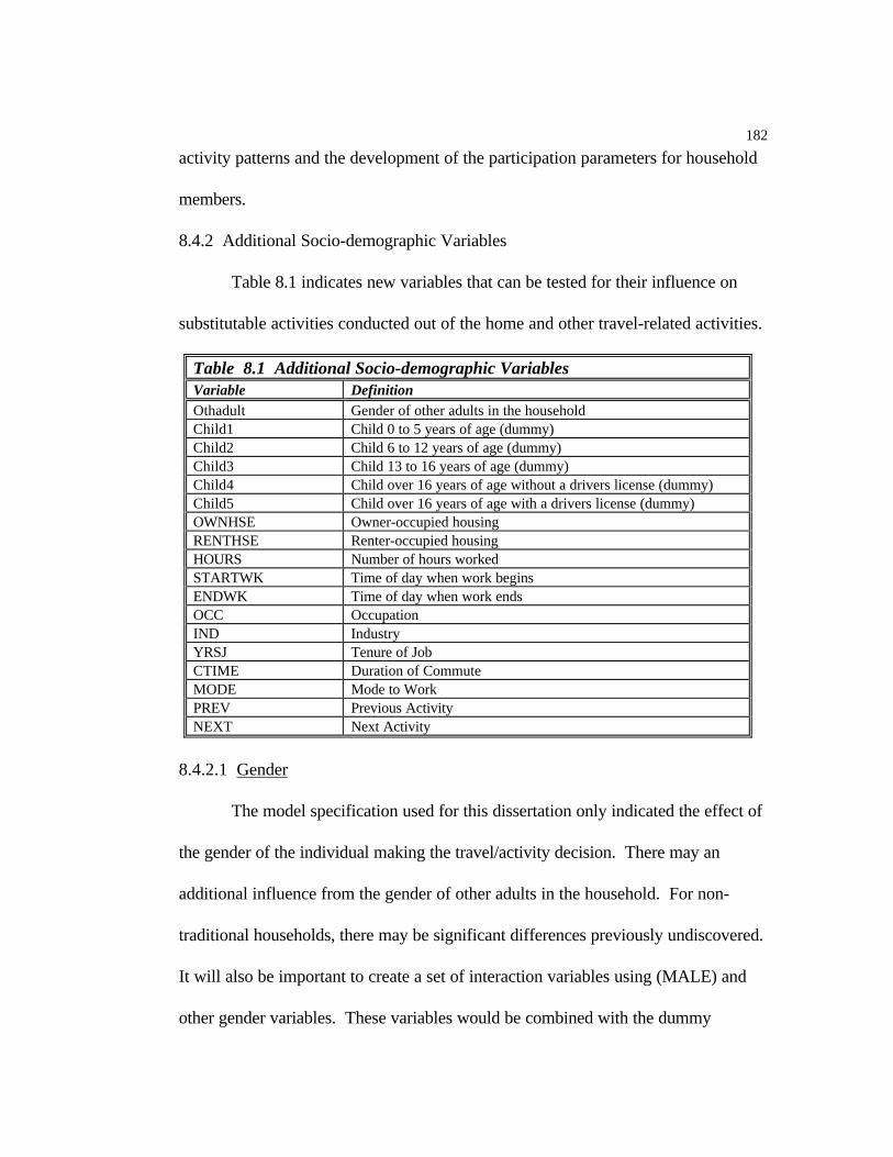
182
activity patterns and the development of the participation parameters for household
members.
8.4.2 Additional Socio-demographic Variables
Table 8.1 indicates new variables that can be tested for their influence on
substitutable activities conducted out of the home and other travel-related activities.
Table 8.1 Additional Socio-demographic VariablesVariable DefinitionOthadult Gender of other adults in the householdChild1 Child 0 to 5 years of age (dummy)Child2 Child 6 to 12 years of age (dummy)Child3 Child 13 to 16 years of age (dummy)Child4 Child over 16 years of age without a drivers license (dummy)Child5 Child over 16 years of age with a drivers license (dummy)OWNHSE Owner-occupied housingRENTHSE Renter-occupied housingHOURS Number of hours workedSTARTWK Time of day when work beginsENDWK Time of day when work endsOCC OccupationIND IndustryYRSJ Tenure of JobCTIME Duration of CommuteMODE Mode to WorkPREV Previous ActivityNEXT Next Activity
8.4.2.1 Gender
The model specification used for this dissertation only indicated the effect of
the gender of the individual making the travel/activity decision. There may an
additional influence from the gender of other adults in the household. For non-
traditional households, there may be significant differences previously undiscovered.
It will also be important to create a set of interaction variables using (MALE) and
other gender variables. These variables would be combined with the dummy

183
variables representing employment status, household size, and other dummies to
determine effects not previously revealed.
8.4.2.2 Household Structure
Future model specifications should consider expanding the understanding of
household structure by including the number and ages of children in the household,
using a dummy variable for their presence. This would increase the understanding
of two-person households that might be made up on a single parent and a child. It
will be necessary to test the appropriate age groupings before establishing the age
brackets. Dummy variables indicating the participation in an activity with others
would need to be interacted with the children-specific variables during various time
periods of the day.
8.4.2.3 Years in the Home
Dummy variables for housing type, either owner (OWNHSE) or rentor
(RENTHSE) status will determine if this difference is important to understanding
the use of travel by individual household members. In addition, the neighhorhood
variables captured through the use of GIS would need to be interacted with housing
type to determine possible additional effects, such as the impact of neighborhood-
specific crime rates on transit use.
To better understand possible effects due to migration, the periods of
residency need to be transformed into dummy variables. These variables can also be
interacted with other socio-demographic factors to identify additional effects.

184
8.4.2.4 Employment Status
Employment status can be expanded to include industry and occupation
information. By interacting industry and occupation information, the nature of the
work experience and its influence on the decision or ability to conduct substitutable
activities out of the home at various times during the day can be examined. Similar
to the concerns over the effect of residential migration, employment changes may
also be an important influence on activities. Job tenure can be categorized into
dummy variables. These dummies may indicate time frames that are more influential
than others and would need to be interacted with other variables for possible
additional effects.
In order to capture the interdependencies between household members,
employment-related variables need to be generated for all adults in a household.
This will allow for the identification of cross-effects. In future data collection
efforts, it would be helpful to gather wage data to better address household
decisions.
8.4.3 Time of Day.
The logit regression coefficients and submodel equivalence tests indicated
that time of day was an important factor with respect to travel/activity decisions.
Additional time periods can be added to the model and tested for statistical
significance. There may be periods of the day when the relevant “time slice” is as
short as fifteen minutes and other periods that are several hours long. This is

185
important to understanding pre- and post- peak travel/activities. It is also important
to obtain a deeper understanding of the nature of off-peak influences, if they are
biased due to activity patterns during the noon hour or other specific time period.
8.4.4 Activity Types and Classifications
In the expansion of the model specification to include activities that require
travel, such as shopping, it will be necessary to test the categorization assumptions.
Unfortunately, as mentioned previously, the data set only represents activities over a
two-day period. As a result, some activities may not be properly represented in the
set. Future research may be able to use other activity data sets (week-long activity
diaries) to enhance the understand of travel/activity behaviors. By using GIS to
control for geographic difference across regions, it may be possible to determine a
generalizable set of travel/activity behaviors.
8.5 CONTRIBUTION TO RESEARCH
The influence of socio-demographic characteristics on travel behavior has
been recognized for several decades. Typically, socio-demographic data is
aggregated, averaged, and applied to transportation zones. The findings of this
dissertation indicate that differences in the probability of making a trip out of the
home for certain activities vary by a number of these socio-demographic
characteristics. In determining the importance of these probabilities to a
transportation system, the percentage of participation in particular activities must be

186
considered. For example, men are 1.62 times more likely than women to participate
in exercise activities out of the home and exercise activities make up 37% of the
leisure activities conducted out of the home.
The insights gained through a better understanding of the use of transport by
individual members of a household has applications for planners. The data indicates
the individuals are more likely to participate in a leisure activity during the morning
and the evening peaks. TDM programs that require “giving-up” the opportunity to
participate in leisure activities are less likely to be successful. However, if
opportunities for leisure activity participation existed at transit locations, the impact
of a shift in modes from single occupant vehicle to transit might not include the loss
of a desired activity type.
The data is not supporting the notion that women are participating in home
production substitutes out of the home during the peaks. This may indicate that the
form of the “substitute” is not the participation in a home production activity out of
the home, but perhaps in the form of the household commodity. In order to obtain
the benefits of participation with other household members, it may be necessary for
activities, such as meals, to continue to occur at home. A “substitutable”
commodity (i.e., ready-to-eat/prepared foods) may reduce the amount of time
necessary to assemble a meal, but the meal location is still within the home.
According to Gray (1998), recent studies in the grocery industry indicate that food
services are the fastest growing share of the grocery industry. Grocery stores are

187
selling “ready-to-eat” meals for individuals to take home for consumption. Gray
(1998) also indicated that individuals are changing their decision-making processes
with respect to food purchases. In the past, shopping was considered on a weekly
basis. In the last decade, this time frame has been shortened to daily shopping.
Survey research is now indicating that by four o’clock in the afternoon, many
individuals do not know what they are having for dinner or where they will be
eating! This real-time decision-making process supports the premise of this
dissertation, that decisions are being made on an activity-by-activity basis, rather
than some predetermined weekly or daily scheduling process.
Incorporating the derived demand for travel is the key to evaluating policy
directives for changing travel behaviors for modeling processes. Until models are
able to identify and report the probability of actual responses, it is unclear how
effective policy evaluations can be made. This dissertation contributes to the
understanding of what activity types, times of day, and specific socio-demographic
characteristics, should be considered for further research.
In order to make these findings operational for transportation forecasting
purposes, they must be incorporated into the next generation of models. Currently,
the focus has been directed to daily activity patterns (McNally 1998; Bowman
1998). To bridge the gap between these two approaches requires the development
of activity webs. An activity web links an activity to a previous and a future activity,
across household members, and time. In this manner, the activity patterns of an
188
individual over an entire day would represent one extreme (one continuous stream
of activities with no links to other individuals), while a complete web might be
represented by a stream of four activities during the morning hours, involving two
household members participating in this set of activities together. In the afternoon,
the decision-making process is separable and is dependent only upon the individual
socio-demographic characteristics of the individual household members. This
approach illustrates the “participation parameter” concept and allows for the
introduction of interdependences among household members.
The household production framework remains the guide for determining
utility for a set of activity webs for an individual household member. This
characterization of activities may lead towards a closer link with the derived demand
for travel, while allowing for integration with current efforts to improve travel
forecasting models.

189
REFERENCES
Abu-Eisheh and Fred Mannering. (1987). “Discrete/Continuous Analysis ofCommuters’ Route and Departure Time Choices.” TransportationResearch Record. 1138: 27-34.
Adler, Thomas and Moshe Ben-Akiva. (1979). “A Theoretical andEmpirical Model of Trip Chaining Behavior.” Transpn. Res. - B.13B: 243-257.
Anas, Alex. (1983). “Discrete Choice Theory, Information Theory and theMultinomial Logit and Gravity Models.” Transpn. Res. - B. 17B(1):13-23.
Banjo, G. Adegboyega and Peter J. B. Brown. (1982). “Patterns of Time-Budget Expenditures in Nigeria.” Transportation Research Record.879: 1-9.
Barber, Gerald. (1986). “Aggregate Characteristics of Urban Travel.” InThe Geography of Urban Transportation, (ed.) Susan Hanson, NewYork: The Guilford Press, pp. 73-90.
Barrett, Christopher, Riko R. Jacob, and Madhav V. Marathe. (1998).“Formal Language Constrained Path Problems.” An unpublishedpaper.
Baumol, William and Alan S. Blinder. (1985). Economics: Principles andPolicy. San Diego, CA: Harbourt Brace Jovanovich, Inc.
Becker, G. S. (1965). “A Theory of the Allocation of Time.” TheEconomic Journal. 75: 493-517.
Becker, G. S. (1976). The Economic Approach to Human Behavior.Chicago, IL: The University of Chicago.
Beckman, Richard J. et al. (1996). “Creating Synthetic BaselinePopulations.” Transpn. Res. - A. 30(6): 415-429.

190
Beckman, Richard et al. (1997). “The Dallas-Ft. Worth Case Study.Transportation Ananlysis SIMulation System (TRANSIMS)”, Release1.0, LAU-97-4502.
Berk, Richard A. (1980). “The New Home Economics: An Agenda forSociological Research.” In Women and Household Labor, (ed.),Sarah Fenstermaker Berk, Beverly Hills, Ca: Sage Publications.
Bernard, Anne, et al. (1996). “Household Structure and Mobility Patternsof Women in O-D Surveys: Methods and Results Based on the CaseStudies of Montreal and Paris.” A paper presented at the SecondNational Conference on Women’s Travel Issues, in Baltimore,Maryland, on October 24-26, 1996.
Bhat, Chandra. (1998). “Joint Model of Work Mode Choice, EveningCommute Stops, and Post-Home-Arrival Stops.” A paper presentedat the 77th Annual Meeting of the Transportation Research Board inWashington, D. C., on January 11 - 15, 1998.
Bhat, Chandra and Frank S. Koppelman. (1993). “An EndogenousSwitching Simulataneous Equation System of Employment, Incomeand Car Ownership.” Transpn. Res.-A. 27A(6): 447-459.
Bianco, Martha and Catherine Lawson. (1996). “Trip-Chaining, Childcare,and Personal Safety: Critical Issues in Women’s Travel Behavior”.A paper presented at the Second National Conference on Women’sTravel Issues in Baltimore, Maryland, on October 24 - 26, 1996.
Blau, Francine D. and Marianne A. Ferber. (1992). The Economics ofWomen, Men, and Work. Englewood Cliffs, NJ: Prentice-Hall.
Boarnet, Marlon G. and Sharon Sarmiento. (1998). “Can Land-use PolicyReally Affect Travel Behavior? A Study of the Link between Non-work Travel and Land-use Characteristics.” Urban Studies. 35(7):1155-1169.
Boulding, Kenneth E. (1966). Economic Analysis. New York, NY:Harper & Row.

191
Bowman, John L. (1998). “The Day Activity Schedule Approach to TravelDemand Analysis.” An unpublished dissertation.
Bowman, John L. and Moshe Ben-Akiva. (1997). “Activity-Based TravelForecasting.” In the Proceedings for Activity-Based TravelForecasting Conference, Travel Model Improvement Program, June2 - 5, 1996.
Bradley, Mark. (1998). “Progress Report on the Activity GeneratorPrototype.” A memo.
Browning, Edgar K. and Jacquelene M. Browning. (1989). MicroeconomicTheory and Applications. Glenview, IL: Scott, Foresman andCompany.
Cambridge Systematics, Inc. (1996). Data Collection in the Portland,Oregon Metropolitan Area. U.S. Department of Transportation.
Chumak, A. and J. P. Braaksma. (1980). “Implications of the Travel-TimeBudget for Urban Transportation Modeling In Canada.”Transportation Research Record. 794: 19-27.
Crown, William H. (1998). Statistical Models for the Social and BehavioralSciences. Westport CT: Praeger Publishers.
Damm, David. (1980). “Interdependencies in Activity Behavior.”Transportation Research Record. 750: 33-40.
Davidson, D. (1991). “Impact of Suburban Employee Trip Chaining onTransportation Demand Management.” Transportation ResearchRecord. 1321: 82-89.
Demaris, Alfred. (1992). Logit Modeling Practical Applications. NewburyPark, CA: Sage Publications.
DeSerpa, A. C. (1971). “A Theory of Economics of Time.” The EconomicJournal. 81: 828-846.
Doherty, Sean T. and Eric J. Miller. (1998). “Activity Patterns fom One-Week Household Activity Scheduling Survey.” A paper presented atthe 77th Annual Meeting of the Transportation Research Board inWashington, D. C., on January 11 - 15, 1998.

192
Downs, Anthony. (1992). Stuck in Traffic: Coping with Peak-Hour TrafficCongestion. Washington, D.C.: The Brookings Institution.
Evans, Alan W. (1972) “On the Theory of the Valuation and Allocation ofTime.” Scottish Journal of Political Economy. 19: 1-17.
Garrett, Mark and Martin Wachs. (1996). Transportation Planning on Trial:The Clean Air Act and Travel Forecasting. Thousand Oaks, CA:Sage Publications.
Gifford, Jonathan L. (1984). “The Innovation of the Interstate HighwaySystem.” Transpn. Res. -A. 18A(4): 319-332.
Golob, Thomas F. (1986). “A Nonlinear Canonical Correlation Analysis ofWeekly Trip Chaining Behavior.” Transpn. Res. - A. 20A: 385-399.
Golob, T. F., M. J. Beckman, and Y. Zahavi. (1981). “A Utility-thoeryTravel Demand Model Incorporating Travel Budgets.” Transpn.Res. -B. 15B(6): 375-389.
Golob, Thomas F., Seyoung Kim, and Weiping Ren. (1994). “A StructuralModel of Vehicle Use in Two-Vehicle Households.” A WorkingPaper, UUCTC No. 224, The University of California TransportationCenter, University of California, Berkeley, Ca.
Golob, Thomas F. and Michael G. McNally. (1995). “A Model ofHousehold Interactions in Activity Participation and the DerivedDemand for Travel.” Presented at the Conference on Activity-basedApproaches: Activity Scheduling and the Analysis of ActivityPatterns, held at the Eindhoven University of Technology, theNetherlands, May 25-28, 1995.
Goodwin, P. B. (1981). “The Usefulness of Travel Budgets.” Transpn.Res. - A. 15A: 97-106.
Gordon, Peter, Ajay Kumar, and Harry W. Richardson. (1988). “Beyondthe Journey to Work.” Transpn. Res. - A. 22A: 416-426.
Gordon, Peter, Ajay Kumar, and Harry W. Richardson. (1989). “GenderDifferences in Metropolitan Travel Behavior.” Regional Studies.23(6): 499-510.

193
Gordon, Peter, Yu-chun Liao, and Harry Richardson. (1994). “HouseholdCommuting.” A paper presented at the Bilateral Seminar, NetworkInfrastructure and the Urban Environment: Recent Advances inLand-Use/Transportation Modeling, Stockholm, Sweden, August1994.
Goulias, Konstandinos and Ryuichi Kitamura. (1989). “Recursive ModelSystem for Trip Generation and Trip Chaining.” TransportationResearch Record. 1236: 59-66.
Graham, John W. and Carole A. Greene. (1984). “Estimating theParameters of a Household Production Function with JointProducts.” The Review of Economics and Statistics. 66(2): 277-282.
Gramm, Wendy Lee. (1975). “Household Utility Maximization and theWorking Wife.” The American Economic Review. 65(1): 90-100.
Gray, John. (1998). “Future Trends in the Changing Food Industry.” Apaper presented at the Fourth Annual Food Industry LeadershipConference, held in Portland, Oregon, on October 27, 1998.
Gronau, Reuben. (1977). “Leisure, Home Production, and Work - theTheory of the Allocation of Time Revisited.” Journal of PoliticalEconomy. 85(6): 1099-1123.
Gronau, Reuben. (1986). “Home Production - A Survey.” In: O.Handbook of Labor Economics, (eds.) Ashenfleter and R. LayardElsevier Science Publishers BV, pp. 273-304.
Gunn, Hugh F. (1981). “Travel Budgets- A Review of Evidence andModeling Implications.” Transpn. Res. -A. 15A: 7-23.
Hamed, Mohammad M. and Fred L. Mannering. (1993). “ModelingTravelers' Postwork Activity Involvement: Toward A NewMethodology.” Transportation Science. 27(4): 381-394.
Hanson, Susan and Margo Schwab. (1986). “Describing DisaggregateFlows: Individual and Household Activity Patterns.” In TheGeography of Urban Transportation, (ed.) Susan Hanson, NewYork: The Guilford Press, pp. 154-178.

194
Hanson, Susan and Perry Hanson. (1981). “The Impact of MarriedWomen's Employment on Household Travel Patterns: A SwedishExample.” Transportation. 10: 165-183.
Hubbard, Raymond. (1978). “A Review of Selected Factors ConditioningConsumer Travel Behavior.” Journal of Consumer Research. 5: 1-21.
Isard, Walter. (1956). Location and Space-Economy. Cambridge,Massachusetts: The M. I. T. Press.
James, Harvey S., Jr. (1996). “The Valuation Of Household Production:How Different are the Opportunity Cost and Market Price ValuationMethods?” Working Paper Series (JEL D13), West Hartford, CT:University of Hartford.
Jara-Diaz, Sergio R. (1998). “A General Micro-Model of Users’ Behavior:The Basic Issues.” In Travel Behaviour Research: Updating theState of the Play, (eds.) J. de D. Ortuzar, S. Jara-Diaz, and D.Hensher, Elsevier.
Khisty, C. Jotin and B. Kent Lall. (1998). Tranportation Engineering: AnIntroduction. Upper Saddle River, New Jersey: Prentice Hall.
Kitamura, R. (1984a). “A Model of Daily Time Allocation to Discretionaryout-of-home Activities and Trips.” Transpn. Res. -B, 18B: 255-266.
Kitamura, R. (1984b). “Incorporating Trip Chaining into Analysis ofDestination Choice.” Transpn. Res. -B, 18B: 67-81.
Kitamura, R. (1988). “An Evaluation of Activity-based Travel Analysis.”Transportation. 15: 9-34.

195
Kitamura, R. (1997). “Applications of Models of Activity Behavior forActivity Based Demand Forecasting.” In the Proceedings for theActivity-Based Travel Forecasting Conference, Travel ModelImprovement Program, New Orleans, LA, June 2 - 5, 1996.
Kitamura, R. and M. Kermanshah. (1983). “Identifying Time and HistoryDependencies of Activity Choice.” Transportation Research Record.944: 22-30.
Kitamura, Ryuichi, Lidia P. Kostyniuk and Michael J. Uyeno. (1980).“Basic Properties of Urban Time-Space Paths: Empirical Tests.”Transportation Research Record. 794: 8-19.
Kitamura, Ryuichi et al. (1996). “The Sequenced Activity MobilitySimulator (SAMS): an Integrated Approach to ModelingTransportation, Land Use and Air Quality.” Transportation. 23:267-291.
Kohlhase, Janet E. (1986). “Labor Supply and Housing Demand for One-Two-Earner Households.” The Review of Economics and Statistics.68(1): 48-56.
Koppelman, F. S. and T. A. Townsend. (1987). “Task Allocation amongHousehold Members: Theory and Analysis.” Paper presented at the5th International Conference on Travel Behavior, Aixen-Provence,France.
Koppelman, Frank S. and Chieh-Hua Wen. (1998). “Different Nested LogitModels: Which Are You Using?” A paper presented at the 77thAnnual Transportation Research Board Meeting in Washington,D.C., January 11- 15, 1998.
Kooreman, Peter and Arie Kapteyn. (1987). “A Disaggregated Analysis ofthe Allocation of Time within the Household.” Journal of PoliticalEconomy. 95(2): 223-249.
Kostyniuk, Lidia P. and Ryuichi Kitamura. (1982). "Life Cycle andHousehold Time-Space Paths: Empirical Investigation."Transportation Research Record. 879: 28-37.
Kraan, Mariette. (1996). Time to Travel? An unpublished dissertation.

196
Lamm, R. McFall, Jr. (1982). “The Demand for Food Consumed at Homeand Away from Home.” Agricultural Economics Research. 34(3):15-20.
Landrock, John N. (1981). “Spatial Stability of Average Daily TravelTimes and Trip Rates Within Great Britain.” Transpn. Res. -A. Vol15A: 55-62.
Lawson, Catherine. (1997). “Household Travel-Activity Decisions: InitialFindings.” A paper presented at the Western Economics AssociationConference held in Seattle, Washington, October, 1997.
Lerman, Steven R. and Charles F. Manski. (1979). “Sample Design forDiscrete Choice Analysis of Travel Behavior: The State of the Art.”Transpn. Res. -A. 13A: 29-44.
Liao, Tim F. (1994). Interpreting Probability Models: Logit, Probit, andOther Generalized Linear Models. Thousand Oaks, CA: SAGEPublications.
Louviere, Jordan. (1994). “Conjoint Analysis”. In Handbook of MarketingResearch, (ed.) R. Bagozzi, Blackwell Publishers.
Lundberg, Shelly and Robert A. Pollak. (1993). “Separate SpheresBargaining and the Marriage Market.” Journal of Political Economy.101(6): 988-1010.
Madden, Janice Fanning. (1981). “Why Women Work Closer to Home.”Urban Studies. 8: 181-194.
Manser, Marilyn and Murray Brown. (1993). “Marriage and HouseholdDecision-Making: A Bargaining Analysis.” International EconomicReview. 21(1): 31-44.
McDonald, K. G. and P. R. Stopher. (1983). “Some Contrary Indicationsfor the Use of Household Structure in Trip-generation Analysis.”Transportation Research Record. 944: 92-100.
McLafferty, Sara and Valerie Preston. (1991). “Gender, Race, andCommuting Among Service Sector Workers.” ProfessionalGeographer. 43(1): 1-15.

197
McNally, Michael. (1998). “Activity-based Forecasting Models IntegratingGIS.” A paper presented at Portland State University, Portland,Oregon.
McNally, Michael. (1995). “An Activity-based Microsimulation Model forTravel Demand Forecasting.” A paper presented at the Activity-based Approaches Conference in Eindhoven, The Netherlands onMay 25-28, 1995.
McNally, Michael and William Recker. (1986). “On the Formation ofHousehold Travel/Activity Patterns: A Simulation Approach.”Final Report under U. S. DOT, Contract No. DTRS-57-81-C-0048.University of California, Irvine.
METRO. (1994). “Oregon and Southwest Washington 1994 Activity andTravel Behavior Survey.” Travel Forecasting Section, Metro,Portland, Oregon.
Meyer, M. D. and Miller, E. J. (1984). Urban Transportation Planning: ADecision-Oriented Approach. Evanston, IL: NorthwesternUniversity Press.
Meurs, Henk. (1993). “A Panel Data Switching Regression Model ofMobility and Car Ownership.” Transpn. Res.-A. 27A(6): 461-476.
Miller, Carole F. (1993). “Part-time Participation Over the Life CycleAmong Married Women Who Work in the Market.” AppliedEconomics. 25: 91-99.
Nicholson, Walter. (1995). Microeconomic Theory: Basic Principles andExtensions. Fort Worth, Texas: The Dryden Press.
Niemeier, D. A. and J. Morita. (1994). “Duration of Trip-Making Activitiesby Men and Women: A Survival Analysis.” Presented at the AnnualMeeting of the Transportation Research Board, Washington, D. C.,January, 1994.
Nishii, Kazuo, Katsunao Kondo, and Ryuichi Kitamura. (1988). “EmpiricalAnalysis of Trip Chaining Behavior.” Transportation ResearchRecord. 1203:48-59.

198
Noland, Robert B. and Kenneth A. Small. (1994). “Travel-timeUncertainty, Departure Time Choice, and the Cost of the MorningCommute.” Presented at the Annual Meeting of the TransportationResearch Board, Washington, D. C., January, 1995.
Oates, Wallace. (1972). Fiscal Federalism. New York, NY: HarcourtBrace Jovanovich, Inc.
Ortuzar, J. de D. and L. G. Willumsen. (1994). Modelling Transport. NewYork, NY: John Wiley and Sons.
Oster, Clinton V. (1978). “Household Tripmaking to Multiple Destinations:The Overlooked Urban Travel Pattern.” Traffic Quarterly. 32: 511-529.
Oster, Clinton V., Jr. (1979). “Second Role of the Work Trip - VisitingNonwork Destinations.” Transportation Research Record. 728: 79-89.
Pas, E. I. (1984). “The Effect of Selected SociodemographicCharacteristics on Daily Travel-Activity Behavior.” Environmentand Planning A. 16: 571-581.
Pas, Eric I. (1986). “The Urban Transportation Planning Process.” In TheGeography of Urban Transportation, ed. Susan Hanson, New York:The Guilford Press, pp. 49-70.
Pas, Eric I. (1997). “Recent Advances in Activity-Based Travel DemandModeling.” A paper in the Proceedings of the Conference onActivity-Based Travel Forecasting held in New Orleans, LA, June 2-5, 1996.
Pazy, Asya, Ilan Salomon, and Tovi Pintizov. (1996). “The Impacts ofWomen’s Careers on their Commuting Behavior: A Case Study ofIsraeli Computer Professionals.” Transpn. Res.-A. 30(4): 269-286.
Pipkin, John S. (1986). “Disaggregate Travel Models.” In The Geographyof Urban Transportation, ed. Susan Hanson, New York: TheGuilford Press, pp. 179-206.
Pisarski, Alan E. (1996). Commuting in America II. Lansdowne, Virginia:ENO Foundation.

199
Pollack, Richard A. and Michael L. Wachter. (1975). “The Relevance ofthe Household Production Function and Its Implications for theAllocation of Time.” Journal of Political Economy. 83(2):255-277.
Prendergast, Lynn S. and Robert D. Williams. (1981). “Individual TravelTime Budgets.” Transpn. Res. -A. 15A: 39-46.
Prevedouros, P. and J. L. Schofer. (1991). “Trip Characteristics and TravelPatterns of Suburban Residents.” Transportation Research Record.1328: 49-57.
Redman, Barbara J. (1980). “The Impact of Women's Time Allocation onExpenditure for Meals Away from Home and Prepared Foods.” Am.J. Agr. Econ. 62(2): 234-237.
Richardson, Harry W. and Peter Gordon. (1989). “Counting NonworkTrips.” Urban Land. 48(9): 6-12.
Robinson, John P. (1977). How Americans Use Time: A Social-Psychological Analysis of Everyday Behavior. New York: Praeger.
Robinson, John P., Vladimir G. Andreyenkov, and Vasily D. Patrushev.(1988). The Rhythm of Everyday Life: How Soviet and AmericanCitizens Use Time. Boulder, CO: Westview Press.
Rosenbloom, S. (1987). “The Impact of Growing Children on TheirParents' Travel Behavior: A Comparative Analysis.” TransportationResearch Record. 1135: 17-25.
Rosenbloom, S. and Elizabeth Burns. (1994). “Why Employed Womenwith Children Need Their Cars; A Pessimistic Look at the Possibilityof Reducing Auto Use.” A paper prepared for the 1994 Conferenceof the Association of Collegiate Schools of Planning.
Schor, Juliet B. (1992). The Overworked American. New York:BasicBooks.
Small, Kenneth A. (1982). “The Scheduling of Consumer Activities: WorkTrips.” American Economic Review. 72(3): 467-479.

200
Small, Kenneth A. (1992). Urban Transportation Economics. Chur,Switzerland: Harwood Acadmic Publishers.
Spear, Bruce. (1996). “New Approaches to Transportation ForecastingModels.” Transportation. 23: 215-240.
Strathman, James G. and Kenneth J. Dueker. (1995). “Understanding TripChaining.” In Special Reports on Trip and Vehicle Attributes." U.S. Department of Transportation.
Strathman, James G., Kenneth J. Dueker and Judy S. Davis. (1993).Congestion Management: Travel Behavior and the Use of ImpactFees, Volume I: Effects of Household Structure and Selected TravelCharacteristics on Trip Chaining. Seattle, WA: TransportationNorthwest (Transnow).
Supernak, Janusz. (1982). “Travel-Time Budget: A Critique.”Transportation Research Record. 879: 15-28.
Train, Kenneth and Daniel McFadden. (1978). “The Goods/LeisureTradeoff and Disaggregate Work Trip Mode Choice Models.”Transportation Research. 12: 349-353.
Wachs, M. (1987). “Men, Women, and Wheels: The Historical Basis ofSex Differences in Travel Patterns.” Transportation ResearchRecord. 1135: 10-16.
Wales T. J. and A. D. Woodland. (1977). “Estimation of the Allocation ofTime for Work. Leisure, and Housework.” Econometrica. 35(1):115-132.
Wang, James Jixian. (1996). “Timing Utility of Daily Activities and itsImpact on Travel.” Transpn. Res. - A. 30(3): 189-206.
Weiner, Edward. (1997). Urban Transportation Planning in the UnitedStates: An Historical Overview. Washington, D.C.: TechnologySharing Program, Research and Special Programs Administration,US Department of Transportation.
Wigan, M. R. and J. M. Morris. (1981). “The Transport Implications ofActivity and Time Budget Constraints.” Transpn. Res. -A. 15: 63-86.

201
Wilson, Paul W. (1989). “Scheduling Costs and the Value of Travel Time.”Urban Studies. 26: 356-366.
Wineberg, Howard and James McCarthy. (1993). “Separation andReconciliation in American Marriages.” Journal of Divorce andRemarriage. 20: 21-42.
Zahavi, Yacov. (1982). “Discussion.” Transportation Research Record.879: 25-28.
Zahavi, Yacov and James M. Ryan. (1980). “Stability of TravelComponents over Time.” Transportation Research Record. 750:19-26.
Zahavi, Yacov and Antti Talvities. (1980). “Regularities in Travel Time andMoney Expenditures.” Transportation Research Record. 750: 13-19.