Hop Doubling Label Indexing for Point-to-Point DistanceQuerying on Scale-Free Networks

Minhao Jiang†, Ada Wai-Chee Fu‡, Raymond Chi-Wing Wong†, Yanyan Xu‡

†The Hong Kong University of Science and Technology ‡The Chinese University of Hong Kongmjiangac, raywong@cse.ust.hk adafu, yyxu@cse.cuhk.edu.hk

ABSTRACTWe study the problem of point-to-point distance querying for mas-sive scale-free graphs, which is important for numerous applica-tions. Given a directed or undirected graph, we propose to buildan index for answering such queries based on a novel hop-doublinglabeling technique. We derive bounds on the index size, the com-putation costs and I/O costs based on the properties of unweightedscale-free graphs. We show that our method is much more effi-cient and effective compared to the state-of-the-art techniques, interms of both querying time and indexing costs. Our empiricalstudy shows that our method can handle graphs that are ordersofmagnitude larger than existing methods.

1. INTRODUCTIONWe study the problem of point-to-point distance querying for

massive scale-free networks or graphs. Given a scale-free graphG = (V,E), we aim to answer queries about the distance of ashortest path from a vertexs to a vertext in the graph. Such query-ing is a basic building block in the solutions of many practical prob-lems including page similarity in web graphs, keyword search onRDF graphs [21], and network analysis such as betweenness cen-trality computation [23]. Indirectly it is useful for community de-tection and locating influential users in the network. We give ourproblem definition as follows.

Problem Definition. Let G = (V,E) be a directed unweightedgraph, with vertex setV and edge setE. Each edge(u, v) ∈ Ehas a length ofdistG(u, v) = 1. Given an edge(u, v), we say thatv is anout-neighborof u, andu is an in-neighborof v. A pathp = (v1, ..., vl) is a sequence ofl vertices inV such that for eachvi(1 ≤ i < l), (vi, vi+1) ∈ E. (We also denotep by v1 ; vl.)Thelengthof a pathp, denoted byℓ(p), is the sum of the lengths ofthe edges onp. Givenu, v ∈ V , thedistancefrom u to v, denotedby distG(u, v), is the minimum length of all paths fromu to v. Ifno pathu ; v exists, thendistG(u, v) = ∞. A pathu ; v witha length ofdistG(u, v) is a shortest path fromu to v. We study thefollowing problem: given a static directed unweighted scale-freegraph G = (V,E), construct a disk-based index for processing

This work is licensed under the Creative Commons Attribution-NonCommercial-NoDerivs 3.0 Unported License. To view a copy of this li-cense, visit http://creativecommons.org/licenses/by-nc-nd/3.0/. Obtain per-mission prior to any use beyond those covered by the license.Contactcopyright holder by emailing info@vldb.org. Articles fromthis volumewere invited to present their results at the 40th International Conference onVery Large Data Bases, September 1st - 5th 2014, Hangzhou, China.Proceedings of the VLDB Endowment,Vol. 7, No. 12Copyright 2014 VLDB Endowment 2150-8097/14/08.

point-to-point (P2P) distance queries, where a P2P distance querydist(s, t) is : givens, t ∈ V , finddistG(s, t).

Although distance querying can be readily handled by Dijkstra’salgorithm [16], the emergence of large networks such as social net-works, RDF graphs, and phone networks has created new chal-lenges. The problem of P2P distance querying has been well stud-ied for road networks. Some previous works include [3, 28, 19, 9,27, 29, 31]. For other graph types, many indexing methods havebeen proposed. However, the previous works of [12, 14, 15, 20, 30,33, 34] can only handle relatively small graphs due to high indexconstruction cost and large index storage space. For the 2 largestreal graphs tested in these studies, we have|V |=581K and|E|/|V |= 2.45 [12], and|V | = 694K and|E|/|V | = 0.45 [20], respectively.The more recent works of IS-Label in [18] and the pruned land-mark labeling (PLL) scheme in [7] can handle bigger graphs. Bothare 2-hop labeling methods [15].

Challenges.While the labeling technique has been adopted bythe state-of-the-art indexing algorithms, there are some major chal-lenges related to this technique. The first challenge is thatno exist-ing work has been able to provide a guarantee of a small label size.The total label size isO(|V |2) and in the worst case, this is thesame size as that of a pairwise distance table. For general graphs,it is shown that there exist graphsG = (V,E) for which any 2-hoplabeling index must have a total size ofΩ(|E||V |1/2) [15]. Thishigh index space complexity will be impractical for large graphs.

The second challenge, which is related to the first, is that noex-isting work has been able to give an acceptable bounded complexityon the computation time and the runtime memory space requiredfor the label construction. Most existing works are in-memory al-gorithms and require huge memory consumption. The only existingwork that has bounded memory consumption is IS-Label [18]. IS-Label builds a hierarchy from the given graph by extracting at eachlevel an independent vertex set. The remaining graph at eachstepis augmented with edges to preserve distances among the remain-ing vertices. Labels are constructed top-down in the hierarchy. Thehierarchy need not be completed so that a residual graphGk mayremain in memory and querying is handled by both the labels and abi-Dijkstra search inGk. However, IS-Label has no guarantee of asmall label size, and also no guarantee on the scalability ofthe la-bel construction time. Another problem of IS-Label is that to limitthe number of iterations,k, during the label construction, insteadof building a full index, a residual graphGk is kept in main mem-ory. However, this is not a pure indexing method since it requiresloadingGk before querying, and the size ofGk can be large.

For the existing in-memory algorithms including [15, 33, 20, 7],the time complexity ranges fromO(|V |2) to O(|E||V |). For thePLL scheme in [7], the actual time performance is much betterthantheO(|E||V |) bound. However, PLL is main memory based and

1203

is not scalable because of a breadth first search process for everyvertex and a pruning process that requires the label index toresidein memory. Hence, a very large main memory is needed that notonly can hold the input graph but also the entire label index with ex-tra storage for computation. Using 48GB RAM, the biggest graphreported in [7] to be handled by PLL is a little over 1GB in sizesince the label size is 22GB. Except for IS-Label, all of the abovealgorithms assume that the given graph can fit in memory, whichmay not be true for massive networks. Hence, scalability remains amajor challenge.

We propose a new indexing method for distance querying to meetthe above challenges. Our design is based on the properties of un-weighted scale-free graphs, which are prevalent in the realworld[1, 10, 17, 25]. Important applications such as social networks,web and most of the collected datasets in [1] belong to this type ofgraphs. We offer guaranteed complexity bounds on the label size,the computation costs and I/O costs. With only 4GB RAM, we areable to build an index for a graph of 9GB in size, with hundredsof millions of vertices and edges. Our method is based on a noveliterative process which minimizes the label size growth at each it-eration, leading to highly effective labeling for the index.

Our main contributions are summarized as follows: (1) We pro-pose a novel 2-hop labeling indexing method for P2P distancequerying on unweighted directed graphs, and have developedI/O-efficient algorithms for index construction when the given graphand the index cannot fit in main memory. (2) Based on the proper-ties of unweighted scale-free graphs, we derive the following com-plexity bounds for our index: the index size isO(h|V |), the com-putational cost isO(|V |logM(|V |/M+ log|V |)), and the I/O costis O(|V |log|V |/M × |V |/B), whereh is a small constant,M isthe memory size andB is the disk block size. (3) We verify theperformance of our method with experiments on large real-worldscale-free networks.

The paper is organized as follows. Section 2 discusses the rele-vant properties of scale-free graphs. Section 3 introducesour mainalgorithm Hop-Doubling. Section 4 describes the I/O-efficient al-gorithms. Section 5 introduces the Hop-Stepping strategy for per-formance enhancement. Section 6 is a discussion about the adapta-tions to undirected and weighted graphs, and about the use ofourmethod for general graphs. We report our empirical study in Sec-tion 7, and conclude in Section 8.

2. 2-HOP LABELING FOR SCALE-FREEGRAPHS

The 2-hop labeling technique constructslabelsfor vertices, anda distance query fors, t can be answered by looking up the labelsof s and t only. Eachlabel is a set of label entries and each la-bel entry is a pair(v, d) wherev ∈ V andd is a distance value.We say thatv is a pivot. For a directed graphG = (V,E), wecreate two labelsLin(v) andLout(v) for each vertexv ∈ V sothat if distG(s, t) 6= ∞, then we can find a pivotu such that(u, d1) ∈ Lout(s), (u, d2) ∈ Lin(t) andd1 + d2 = distG(s, t),and there does not exist anyu′ such that(u′, d′1) ∈ Lout(s),(u′, d′2) ∈ Lin(t) andd′1 + d′2 < distG(s, t). We say that the pair(s, t) is coveredby u. Hence, the distance querydist(s, t) can beanswered by looking upLout(s) andLin(t) for such a pivotu withthe smallestd1 + d2.

The set of labels for all vertices is called a2-hop cover. Thecomplexity of finding a minimum 2-hop cover is shown to be NP-hard [15], and known approximate algorithms are also very costly[20]. However, in the following discussion, we will show that cer-tain ordering of vertices may give rise to a good 2-hop cover,whichsheds some light on this hard problem.

Figure 1: A road graph GR

L(a) (a, 0), (b, 1), (c, 2), (d, 1), (e, 1)L(b) (b, 0), (c, 1), (d, 2), (e, 2)L(c) (c, 0), (e, 3)L(d) (d, 0), (c, 3)L(e) (e, 0), (d, 2)

Table 1: A label index for GR

Figure 2: A star graph GS

L(a) (a, 0), (b, 1), (c, 1), (d, 1),(e, 1), (f, 1)

L(b) (b, 0), (c, 2), (d, 2)L(c) (c, 0), (d, 2), (e, 2)L(d) (d, 0), (e, 2), (f, 2)L(e) (e, 0), (f, 2), (b, 2)L(f) (f, 0), (b, 2), (c, 2)

Table 2: A label index for GS

L(a) (a, 0)L(b) (b, 0), (a, 1)L(c) (c, 0), (a, 2), (b, 1)L(d) (d, 0), (a, 1)L(e) (e, 0), (a, 1)

Table 3: A small GR index

L(a) (a, 0)L(b) (b, 0), (a, 1)L(c) (c, 0), (a, 1)L(d) (d, 0), (a, 1)L(e) (e, 0), (a, 1)L(f) (f, 0), (a, 1)

Table 4: A small GS index

2.1 Ordering of Vertices for LabelingThe importance of the ordering of vertices can be illustrated by

some very simple graphs. In Figure 1, we show a graphGR for rep-resenting a simple road system.GR is undirected, but we can treatit as directed since each edge can be seen as bidirectional. Table 1is a 2-hop cover forGR whereL(v) = Lin(v) = Lout(v). The2-hop cover isminimal , meaning that we cannot delete any labelentry and still maintain the correctness of distance query evalua-tion. The entries of the form(v, 0) are trivial but are needed forquery answering. In Figure 2, we show a star graph,GS . Table 2is a 2-hop cover forGS which is also minimal. For example, if wedelete(c, 2) from L(b), then for a query ofdist(b, c), we wouldreturn an incorrect distance of 4 from(d, 2) in L(b) and(d, 2) inL(c). Note that one can add many useless entries to these coversso that they are still correct but not minimal.

For a given graph, there can be many possible minimal 2-hopcovers, and in Tables 3 and 4, we show smaller minimal 2-hopcovers forGR andGS , which reduce the number of non-triviallabel entries by half or more when compared with those shown inTables 1 and 2. Intuitively, for the road network, we are makinguse of the huba, which lies on the shortest paths for many pairsof vertices. Similarly, we make heavy use of the centera of thestar graph, which has a highest degree. The problem of findinga minimum 2-hop cover is to find a smallest set of label entrieswith pivots that cover the shortest paths for answering all distancequeries, and in these special graphs, the hub or center obviouslyhits the most number of shortest paths. We can set a ranking onthevertices in such a way that higher ranked vertices are likelyto hitmore shortest paths, and then use higher ranked vertices forpivots,as in the examples. This should result in a smaller label size.

The above idea is more formally treated by the notion ofcanoni-cal labelingin [4]. If shortest paths are not unique for givens, t, wemay define canonical labeling as follows. Given a total rankingr()of all vertices inV , a labeling is canonical if a vertexv is a pivotin Lout(u) if and only if there exists a vertexw such thatr(v) isthe highest among all vertices in all shortest paths fromu tow, andsimilarly for Lin(u). The labeling is minimal since deleting anypivot creates some uncovered pair of vertices. Canonical labelingcalls for thepruning of any entry(v, d) in Lout(u) if by lookingupLout(u) andLin(v) we find a higher rank pivotv′ that gives a

1204

pathp = (u, ..., v′, ..., v) with a length≤ d. This is because ifv ison a shortest path fromu to another vertexw which is made up ofp′ = (u, ..., v) of lengthd andq = (v, ..., w), thenv′ will also beon a shortest path fromu tow, which is made up ofp andq. Sincer(v′) > r(v), v should not be chosen as a pivot here.

Given the importance of ranking as illustrated in the above ex-amples, we expect good indexing results from a good vertex rank-ing. The independent set approach of IS-Label [18] effectivelygives low ranking to low degree vertices. This ordering is foundto produce good label sizes. The pruned landmark scheme PLL in[7] builds labels for an unweighted graph by a breadth first search(BFS) from vertices ordered in non-increasing degrees. Thesearchfrontiers of BFS are halted at vertices where the label entries arepruned by previously entered entries as described in the above.Note that such pruning has also been proposed in [4]. This orderingby degree is found to be highly effective for many real graphs. Inthe next subsection, we will derive reasons behind this effectivenessfor scale-free graphs. We make use of the definition ofhitting setsand a concept similar to thehighway dimensionintroduced in [5,2] for road networks. However, we should point out that the char-acteristics of a scale-free graph is very much different from that ofa road network.

2.2 Hitting Sets in Scale-free GraphsA function f(x) is said to bescale-freeif f(bx) = C(b)f(x),

whereC(b) is some constant dependent only onb. It is commonto call a graph scale-free if the distribution of vertex degrees of thegraph follows apower law: Prob(a vertex has degreek) ∝ k−α,whereα is a positive real number. This is scale-free since iff(x) =cx−α, thenf(bx) = c(bx)−α = b−αf(x). Typically, 2 ≤ α ≤ 3[13, 11, 17]. Existing works [10, 17, 1, 25] have shown that manyreal world graphs do follow such power law distributions. Based onthe BA model [8] of scale-free graphs, Bollobas et al. [10] provedthat the diameterD of a scale-free random graph is asymptotically

D = log |V |/ log log |V | (1)

Although this is an asymptotical analysis, it gives very accurateprediction for many real world scale-free graphs [1, 32].

Newman et al. [25] studied the properties of scale-free graphsby means of generating functions for the probability distribution ofvertex degrees. Letzi be the average number of vertices that arei hops away from a randomly chosen vertexv. It is shown thatwith very high probability,zm = (z2/z1)

m−1z1. Hencezm =(z2/z1)zm−1. Thus, theexpansion factorR can be determined bythe average number of vertices that are 1 or 2 hops fromv, respec-tively, i.e.,R = z2/z1. With an expansion factor ofR, the diameterof the graph can be estimated to beD = logR|V | = log|V |/logR.From Equation (1), the expansion factor is given by

R = log|V | (2)

For a graphG = (V,E) that follows a power law distribution,Faloutsos et al. [17] derived the following relationship between thedegreedegv of a vertexv in G and its rank in terms of the degree.For a vertexv ∈ V , v has ther(v)-th highest degree inG.

LEMMA 1. [17] The degree,degv, of a vertexv, is a functionof the rank of the vertex,r(v), and the rank exponent,γ, as follows:

degv =1

|V |γ(r(v)γ) (3)

In the above,γ is a small real number found to be between−0.8and−0.7 for many real-world graphs [17]. According to Equation(3), takingγ = −0.8 for a scale-free graphG1 = (V1, E1), if

|V1|=1M, then less than 500 vertices have degree above 500, andthe top-degree vertexv0 has a degree of 63095. From Equation(2), the expansion factor is given byR = log |V1| ≈ 20. Since63095 × 20 > 1M , v0 is expected to reach all vertices within 2hops.

Let us call the number of hops (edges) on a path itshop length.Given a set of pathsP , a hitting set for P is a set of verticesSsuch that each pathp in P contains at least one vertexv in S (wesay thatp is hit by v). For the above graphG1, a single highestdegree vertex is expected to hit all shortest paths with length ≥ 4.In general, we make an assumption of asmall hitting set forlongshortest paths as follows.

ASSUMPTION 1. Given an unweighted scale-free graphG =(V,E), there exist small integersd0 andh, and a setH of the high-est degree vertices inV , such that∀u, v ∈ V , if there exist shortestpathsu ; v with hop length≥ d0, then one such path is hit byone ofh vertices inH.

In Assumption 1,|H| ≥ h. Given Equations (1) to (3), we canshow that Assumption 1 holds withd0 = 4 andh = 1 for anyundirected unweighted scale-free graphG = (V,E) with |V | ≥3, and rank exponent−0.8 ≤ γ ≤ −0.7 (typical values in realworld graphs [17]). The analysis goes as follows. From Lemma1, the degree ofv0 is given by|V |−γ sincer(v0) = 1. With anexpansion factor ofR, if (degv0 × R) ≥ |V |, thenv0 reaches allvertices in 2 hops. This is the case where(|V |−γ · R) ≥ |V |,and from Equation 2,R = log |V |; hence the inequality becomes(|V |−γ−1 · log |V |) ≥ 1, and this holds for all values of|V | ≥ 3for −0.8 ≤ γ ≤ −0.7. Therefore, when|V | ≥ 3, the highestdegree vertex will reach all other vertices in 2 hops, which meansthat each vertex can reach any other vertex within 4 hops. Hence,d0 = 4 andh = 1.

The above analysis is based on undirected unweighted graphs.However, the power law distribution is commonly found in directedgraphs by examining the in-degree and out-degree distribution sep-arately [22, 26]. The study in [25] also considers directed graph,and by focusing on the vertices that can be reached from a randomvertex, it is found that many results follow as in undirectedgraphs.Hence, Assumption 1 is also for directed graphs.

Based ond0, we have two types of shortest paths: long ones (i.e.,those of hop length at leastd0) and short ones (i.e., those of hoplength belowd0). We have identified hitting sets for covering thelong shortest paths based on Assumption 1. Next, we will examinehow the shortest paths of hop length shorter thand0 can be handled.

Let P< be the set of all shortest pathsp such thatℓ(p) < d0,andP≥ be the set of all shortest pathsp such thatℓ(p) ≥ d0.The d0-inner-circle of a vertex v is defined to beN<(v) =p | p ∈ P< ∧ v ∈ p. We can visualizeN<(v) as the set of allshortest paths passing throughv within a ball with radiusd0 cen-tered atv, where each path has length less thand0. Similarly, thed0-outer-circle of v is defined asN≥(v) = p | p ∈ P≥ ∧ v ∈ p.

We define a neighborhood for vertexv to be used as a hitting setfor short shortest paths throughv. LetN(v) = u|distG(v, u) <d0∨distG(u, v) < d0,NH(v) = N(v)∩H, andN ′′(v) ⊆ N(v)be vertices connected toNH(v) so that for any vertexu ∈ N ′′(v),there is a shortest path fromv to u or fromu to v which contains avertex inNH (v). Then, the set of vertices ofNe(v) = ((N(v) −N ′′(v)) ∪NH(v)) is called theH-excluded neighborhood ofv. Ifthere exists a shortest pathp = v ; u with hop length< d0,thenp is hit by a vertexw, wherew ∈ Ne(v) andw ∈ Ne(u).If we include entries for all vertices inNe(v) in the label for eachvertexv, such a shortest path will be found from the labels of the 2

1205

endpoint vertices of the path. We make an assumption thatNe(v)is small.

ASSUMPTION 2. In an unweighted scale-free graphG =(V,E), for a vertexv, theH-excluded neighborhood ofv, Ne(v),contains at mosth vertices.

Given an expansion factor ofR, for a scale free graphG =(V,E), |Ne(v)| for v ∈ V is bounded byRd0−1. If |V | = 1M ,then R ≈ 20, and if −0.8 ≤ γ ≤ −0.7, d0 = 4. Then,|Ne(v)| < 203 = 8000. The actual size of|Ne(v)| is muchsmaller than this bound since high degree vertices cover a largenumber of edges inG and their expansions are excluded inNe(v).

The smallh value assumption is substantiated by our experimen-tal results on a large number of real graphs. We say that a graph hashub dimensionh if ∀u ∈ V,∃ a hitting setH< for N<(u) suchthat |H<| = O(h) and∃ a hitting setH≥ for N≥(u) such that|H≥| = O(h). Intuitively, given hub dimensionh, there existsfor each vertexu a set of at mostO(h) vertices hitting all shortestpaths passing throughu, which bounds the optimal label size ofuby O(h). We state our assumption of small hub dimension.

ASSUMPTION 3. An unweighted scale-free graph has a smallhub dimensionh.

In summary, we provide realistic assumptions for unweighteddirected/undirected scale-free graphs. Based on Assumption 3, theoptimal label size is bounded byO(h) for each vertex. Our empiri-cal study in Section 7 shows that for all the scale-free real-worldand synthetic graphs that we have tested, the label sizes result-ing from our algorithm are very small compared to the graph size.Thus, the assumptions above are strongly supported by experimen-tal results. The remaining question is how to attain this size bound.

2.3 Existing Algorithms with Vertex OrderingAs discussed in Section 2.1, ranking of vertices by their degrees

has been adopted in PLL [7], and less explicitly in IS-Label [18].However, as noted in Section 1, both of these methods are not scal-able. For PLL, the in-memory label construction involves manyiterations of breadth first search (BFS), and BFS does not yield toan efficient external algorithm to date [24]. More importantly, tobe efficient, the label pruning in PLL requires a main memory thatcan hold the labeling index, which is typically much bigger thanthe given graph. Hence, it is an open problem to derive an algo-rithm with scalable bounds on memory and computation consump-tion and that produces bounded index sizes. We will focus on thisproblem for scale-free graphs.

In [13], it is shown that high-degree vertices in power-law graphsare useful for finding approximate shortest paths by a compact rout-ing scheme. Arouting tableis built for each vertexv, which keepstrack of shortest paths to high-degree vertices called landmarks andto vertices closer tov. However, the query evaluation in [13] doesnot return exact answers. In the next sections, we shall makeuse ofvertex degree ordering to derive an I/O efficient algorithm for indexconstruction for exact querying on a large scale-free graph. Our al-gorithm does not require the knowledge ofh but will seamlesslyattain the label size bound ofO(h|V |) and scalable complexities.

3. PROPOSED SOLUTIONOur proposed solution is made up of the three major components

of algorithmic designs. We first give an outline of each component.

1. The basic framework of our label index construction is aniterative process with two steps in each iteration: (i) labelentry generation based on a set of rules; and (ii) label pruningto reduce the label size.

2. The second design component is an I/O efficient algorithmfor implementing the iterative process (see Section 4).

3. The third algorithmic design is an enhancement on the per-formance based on the idea of hop-stepping (see Section 5).

In this section we describe the iterative process of label genera-tion and pruning. Based on the discussion in Section 2.2, we designour labeling algorithm with the assumption that the hittingset of themajority of paths of longer lengths passing through a vertexv is asmall set ofh high degree vertices inH. Since each label entryshould correspond to a shortest path, if we place the entries(vh, d)for verticesvh in H in the relevant vertex labels, they would servemost querying. Analogously, we should try to avoid creatinglabelentries for shortest pathsp = v ; u wherevh is in p for somevertexvh ∈ H, andvh 6∈ u, v. From our assumptions, thereare many such paths, and hence many possible label entries, whichwill lead to large label sizes. We will introduce the notion of troughpathsfor these purposes.

Our strategy is to rank all vertices uniquely according to non-increasing degrees, with the highest rank given to the highest de-gree vertex. Next, our algorithm generates label entries tocovershortest paths with increasing number of hops. There are severalreasons for this strategy. Firstly, we need to search the neighbor-hood of each vertex for the coverage of short shortest paths.Sec-ondly, we need short shortest paths involvingH for pruning otherpaths. Hence, we traverse from short to long paths. Thirdly,theiterative approach can be realized by I/O efficient algorithms withscalable I/O complexities, as we will show in Section 5. We willexplain these points in the following discussion.

3.1 Iterative Labeling AlgorithmGiven a directed unweighted graphG = (V,E), let

v1, v2, ..., vn be a ranking of the vertices inV so that the rankof vi, denoted byr(vi), is equal toi. We rank the vertices in non-increasing order of their vertex degrees. Thus, vertexv1 has thehighest degree. We break ties arbitrarily for vertices withthe samedegree. Next we introduce the notion of a trough shortest path.

DEFINITION 1 (TROUGH SHORTEST PATH). A trough pathfrom v to u is a path passing through only vertices with rankssmaller thanmaxr(u), r(v). A trough shortest path is a troughpath that is also a shortest path.

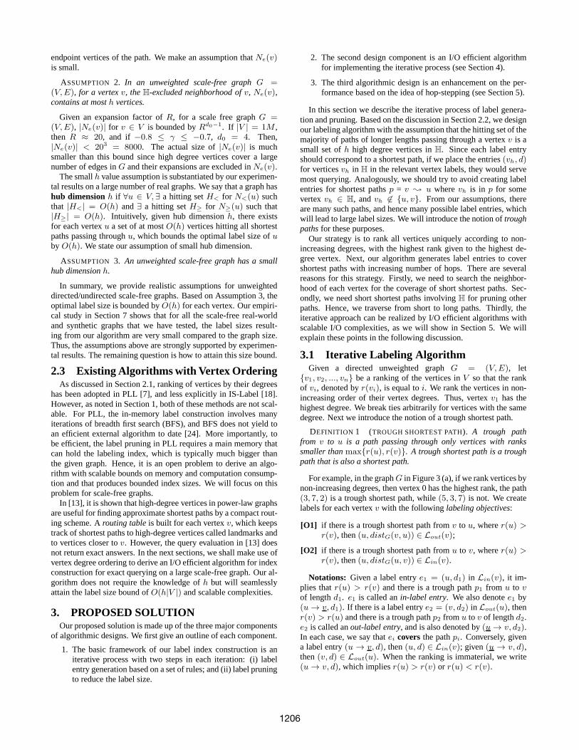
For example, in the graphG in Figure 3 (a), if we rank vertices bynon-increasing degrees, then vertex 0 has the highest rank,the path(3, 7, 2) is a trough shortest path, while(5, 3, 7) is not. We createlabels for each vertexv with the following labeling objectives:

[O1] if there is a trough shortest path fromv to u, wherer(u) >r(v), then(u, distG(v, u)) ∈ Lout(v);

[O2] if there is a trough shortest path fromu to v, wherer(u) >r(v), then(u, distG(u, v)) ∈ Lin(v).

Notations: Given a label entrye1 = (u, d1) in Lin(v), it im-plies thatr(u) > r(v) and there is a trough pathp1 from u to vof lengthd1. e1 is called anin-label entry. We also denotee1 by(u → v, d1). If there is a label entrye2 = (v, d2) in Lout(u), thenr(v) > r(u) and there is a trough pathp2 from u to v of lengthd2.e2 is called anout-label entry, and is also denoted by(u → v, d2).In each case, we say thatei coversthe pathpi. Conversely, givena label entry(u → v, d), then(u, d) ∈ Lin(v); given(u → v, d),then(v, d) ∈ Lout(u). When the ranking is immaterial, we write(u → v, d), which impliesr(u) > r(v) or r(u) < r(v).

1206

0

1 2

34

5 67

(a)

0

1 2

34

5 67

(b)

Figure 3: (a) Given graphG = (V,E) (b) Trough paths coveredafter the first iteration (arrows with dotted lines)

Figure 4: Set of label entries generation rules

In our labeling algorithm, initially each vertexv is assigned twolabelsLin(v) = (v, 0) andLout(v) = (v, 0). In the initial-ization process, for each edge(u, v) ∈ E, if r(u) < r(v), we addlabel entrye = (v, distG(u, v)) to Lout(u); if r(u) > r(v), weadde = (u, distG(u, v)) toLin(v).

Our algorithm iteratively generates label entries for all verticesuntil no more label entries can be formed. The first iterationisthe initialization process. In each remaining iteration, we have aset of new label entries which have been generated in the previousiteration, which we denote byprevLabel. Also we have a set ofall label entries generated from all previous iterations, we refer tothis set asallLabel. In each iteration, we adopt 6 rules repeatedlyto generate all the possible label entries for the iteration. The rulesare encoded in Table 5. The first rule is derived from the first row inthe table as follows:∀(u → v, d) ∈ prevLabel, ∀(u1 → u, d1) ∈allLabel, generate(u1 → v, d1 + d). Similarly, the other 5 rulescan be derived from the table. The rules are illustrated in Figure 4,where each solid or dotted arrow indicates a label entry.

prevLabel allLabel generate

Rule 1 (u → v, d) (u1 → u, d1) (u1 → v, d1 + d)Rule 2 (u → v, d) (u2 → u, d2) (u2 → v, d2 + d)Rule 3 (u → v, d) (v → u3, d3) (u → u3, d3 + d)Rule 4 (u → v, d) (v → u4, d4) (u → u4, d4 + d)Rule 5 (u → v, d) (v → u5, d5) (u → u5, d5 + d)Rule 6 (u → v, d) (u6 → u, d6) (u6 → v, d6 + d)

Table 5: Set of label entry generation rules

A generated label entry(u → v, d) becomes a new label entryfor the current iteration if there is no existing label entryfor u → v,or d is a smaller distance compared with that in other generated orexisting label entries foru → v. When we generate label entrye from two label entriese1 ande2, and given thate1 covers pathp1 = (u1, ..., ui) ande2 covers pathp2 = (ui, ..., uj), then we saythate coversthe path(u1, ..., ui, ..., uj). We shall show that afterevery two iterations, we double the hop length of trough shortestpaths that are covered by the label entries generated. Hence, wecall this methodHop-Doubling Labeling (see Algorithm 1).

EXAMPLE 1. Given the unweighted graph in Figure 3(a). Thevertices are ranked by non-increasing degrees and given ID’s 0 to7 accordingly, i.e., vertex 0 has the highest rank. Hop-DoublingLabeling first creates one label entry for each edge:(0 → 1, 1),(1 → 0, 1), (2 → 0, 1), ... In the first iteration, by Rule 1 or

Lin(0) (0, 0)Lin(1) (1, 0), (0, 1)Lin(2) (2, 0)Lin(3) (3, 0), (2, 1)Lin(4) (4, 0)Lin(5) (5, 0), (4, 1)Lin(6) (6, 0), (0, 1),

(2, 1)Lin(7) (7, 0), (3, 1),

(2, 2)1

Lout(0) (0, 0)Lout(1) (1, 0), (0, 1)Lout(2) (2, 0), (0, 1), (1, 2)1Lout(3) (3, 0), (1, 1), (2, 2)1, (0, 2)1Lout(4) (4, 0), (0, 1), (1, 1), (3, 2)1,

(2, 4)2Lout(5) (5, 0), (3, 1), (1, 2)1, (2, 3)2,

(0, 3)2Lout(6) (6, 0)Lout(7) (7, 0), (2, 1)

Figure 5: Labeling for graph G in Figure 3. The superscript ofan entry indicates the iteration in which the entry is generated.

4, we generate(2 → 1, 2) from (2 → 3, 1) and (3 → 1, 1).Similarly, (4 → 3, 2) and (3 → 2, 2) are generated. By Rule 2or 3, we generate(5 → 1, 2) and (3 → 0, 2), and Rule 5 or 6generates(2 → 7, 2). In the second iteration, Rule 2 generates(4 → 2, 4) from (4 → 3, 2) and(3 → 2, 2), Rule 2 also generates(5 → 2, 3) and (5 → 0, 3). In the third iteration, no new labelentry is generated and the labeling is completed. The resultinglabels are shown in Figure 5.

Algorithm 1: Hop-Doubling Labeling

Input : G = (V, E)Output : (Lin,Lout)

// Initialization1 rank the vertices by non-increasing degrees;2 allLabel = prevLabel = set of labels covering all edgese ∈ E;

// iterative construction3 while prevLabel 6= ∅ do4 UpdateprevLabel, allLabel using the set of label entry

generation rules;

5 build index of(Lin,Lout) from allLabel;

Next, we show that distance querying based on the labels con-structed by the algorithm is correct. First, we need a lemma.

LEMMA 2. Hop-Doubling labeling achieves the labeling ob-jectives of[O1] and[O2] given in Section 3.1.

PROOF: Consider a trough shortest pathp from v to u. Let thepath bep = (v = w1, w2, ..., wk = u). We show by inductionon the hop length ofP . The base case is trivial since we alwaysinclude(v, 0) in Lin(v) andLout(v). Next, assume the statementsin [O1] and[O2] true for all paths of hop length 1 tok−1. Considerthe pathp = (v = w1, w2, ..., wk = u). There are two possiblecases. Case A :r(wk) > r(w1); Case B:r(w1) > r(wk). Letuse first consider Case A. Letr(wi) > r(wj) for all j < k andj 6= i. Sincep is a shortest path fromv to u, the sub-pathp1= (w1, ..., wi) must be a shortest path fromw1 to wi. Similarly,the sub-pathp2 = (wi, ..., wk) is a shortest path fromwi to wk.Clearly,distG(w1, wk) = distG(w1, wi)+distG(wi, wk). Sincer(wi) is the second highest rank inp, both p1 andp2 are troughshortest paths. There are two subcases:

Case A1 :r(wi) < r(w1) < r(wk). By the induction hypoth-esis,e1 = (wk, distG(wi, wk)) will be inserted intoLout(wi),and e2 = (w1, distG(w1, wi)) will be inserted intoLin(wi).Note thate1 = (wi → wk, distG(wi, wk)) and e2 = (w1 →wi, distG(w1, wi)). e1 ande2 may be inserted at the same itera-tion or at different iterations. Ife1 is inserted in a later round thane2, then by Rule 1,e3 = (wk, distG(w1, wi) + distG(wi, wk))for Lout(w1) will be generated. Ife2 is inserted in a later round,then by Rule 4,e3 will be generated forLout(w1).

1207

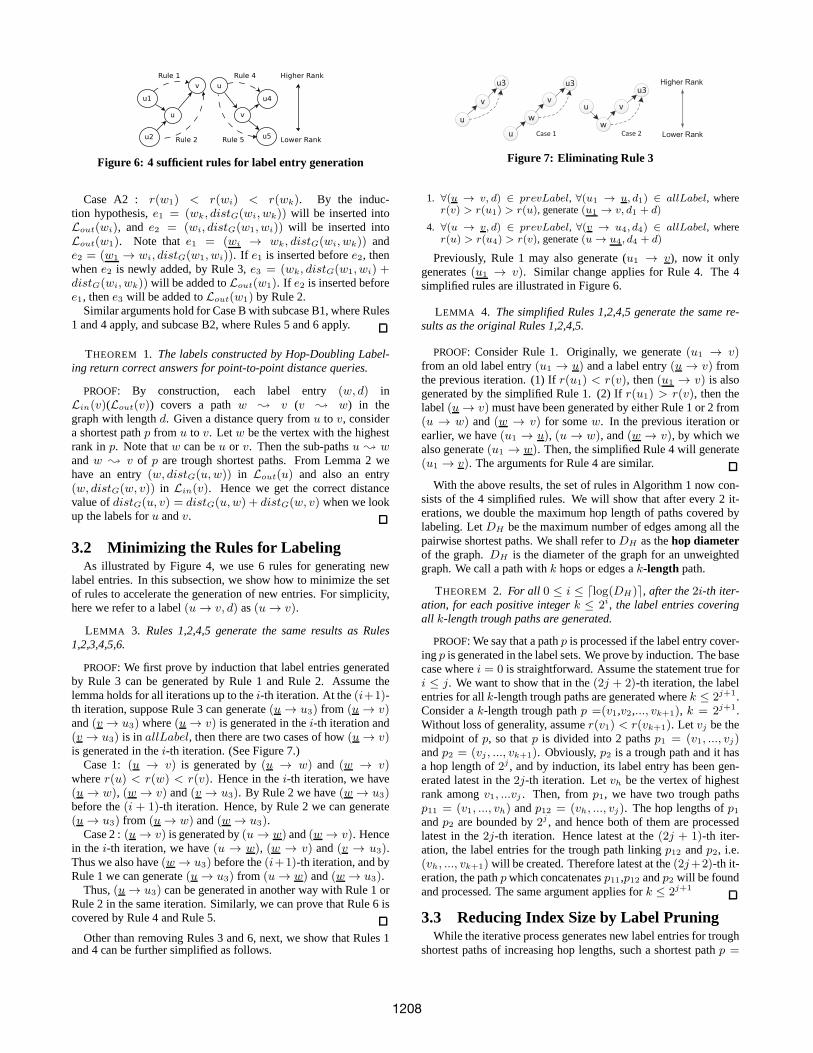
Figure 6: 4 sufficient rules for label entry generation

Case A2 : r(w1) < r(wi) < r(wk). By the induc-tion hypothesis,e1 = (wk, distG(wi, wk)) will be inserted intoLout(wi), and e2 = (wi, distG(w1, wi)) will be inserted intoLout(w1). Note thate1 = (wi → wk, distG(wi, wk)) ande2 = (w1 → wi, distG(w1, wi)). If e1 is inserted beforee2, thenwhene2 is newly added, by Rule 3,e3 = (wk, distG(w1, wi) +distG(wi, wk)) will be added toLout(w1). If e2 is inserted beforee1, thene3 will be added toLout(w1) by Rule 2.

Similar arguments hold for Case B with subcase B1, where Rules1 and 4 apply, and subcase B2, where Rules 5 and 6 apply.

THEOREM 1. The labels constructed by Hop-Doubling Label-ing return correct answers for point-to-point distance queries.

PROOF: By construction, each label entry(w, d) inLin(v)(Lout(v)) covers a pathw ; v (v ; w) in thegraph with lengthd. Given a distance query fromu to v, considera shortest pathp from u to v. Letw be the vertex with the highestrank inp. Note thatw can beu or v. Then the sub-pathsu ; wandw ; v of p are trough shortest paths. From Lemma 2 wehave an entry(w, distG(u,w)) in Lout(u) and also an entry(w, distG(w, v)) in Lin(v). Hence we get the correct distancevalue ofdistG(u, v) = distG(u,w) + distG(w, v) when we lookup the labels foru andv.

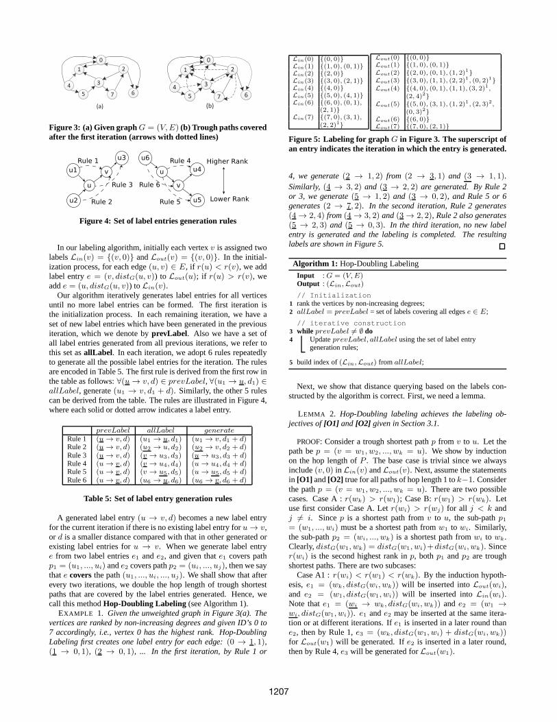
3.2 Minimizing the Rules for LabelingAs illustrated by Figure 4, we use 6 rules for generating new

label entries. In this subsection, we show how to minimize the setof rules to accelerate the generation of new entries. For simplicity,here we refer to a label(u → v, d) as(u → v).

LEMMA 3. Rules 1,2,4,5 generate the same results as Rules1,2,3,4,5,6.

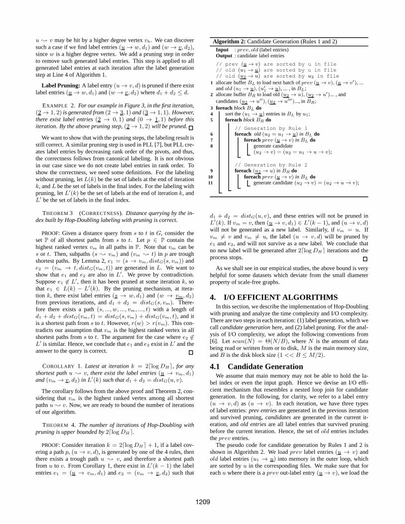
PROOF: We first prove by induction that label entries generatedby Rule 3 can be generated by Rule 1 and Rule 2. Assume thelemma holds for all iterations up to thei-th iteration. At the(i+1)-th iteration, suppose Rule 3 can generate(u → u3) from (u → v)and(v → u3) where(u → v) is generated in thei-th iteration and(v → u3) is in allLabel, then there are two cases of how(u → v)is generated in thei-th iteration. (See Figure 7.)

Case 1: (u → v) is generated by(u → w) and (w → v)wherer(u) < r(w) < r(v). Hence in thei-th iteration, we have(u → w), (w → v) and(v → u3). By Rule 2 we have(w → u3)before the(i + 1)-th iteration. Hence, by Rule 2 we can generate(u → u3) from (u → w) and(w → u3).

Case 2 :(u → v) is generated by(u → w) and(w → v). Hencein the i-th iteration, we have(u → w), (w → v) and(v → u3).Thus we also have(w → u3) before the(i+1)-th iteration, and byRule 1 we can generate(u → u3) from (u → w) and(w → u3).

Thus,(u → u3) can be generated in another way with Rule 1 orRule 2 in the same iteration. Similarly, we can prove that Rule 6 iscovered by Rule 4 and Rule 5.

Other than removing Rules 3 and 6, next, we show that Rules 1and 4 can be further simplified as follows.

u3

v v

wu

u

u3

Case 1

Higher Rank

v

w

u

u3

Case 2 Lower Rank

Figure 7: Eliminating Rule 3

1. ∀(u → v, d) ∈ prevLabel, ∀(u1 → u, d1) ∈ allLabel, wherer(v) > r(u1) > r(u), generate(u1 → v, d1 + d)

4. ∀(u → v, d) ∈ prevLabel, ∀(v → u4, d4) ∈ allLabel, wherer(u) > r(u4) > r(v), generate(u → u4, d4 + d)

Previously, Rule 1 may also generate (u1 → v), now it onlygenerates(u1 → v). Similar change applies for Rule 4. The 4simplified rules are illustrated in Figure 6.

LEMMA 4. The simplified Rules 1,2,4,5 generate the same re-sults as the original Rules 1,2,4,5.

PROOF: Consider Rule 1. Originally, we generate(u1 → v)from an old label entry(u1 → u) and a label entry(u → v) fromthe previous iteration. (1) Ifr(u1) < r(v), then(u1 → v) is alsogenerated by the simplified Rule 1. (2) Ifr(u1) > r(v), then thelabel(u → v) must have been generated by either Rule 1 or 2 from(u → w) and(w → v) for somew. In the previous iteration orearlier, we have(u1 → u), (u → w), and(w → v), by which wealso generate(u1 → w). Then, the simplified Rule 4 will generate(u1 → v). The arguments for Rule 4 are similar.

With the above results, the set of rules in Algorithm 1 now con-sists of the 4 simplified rules. We will show that after every 2it-erations, we double the maximum hop length of paths covered bylabeling. LetDH be the maximum number of edges among all thepairwise shortest paths. We shall refer toDH as thehop diameterof the graph.DH is the diameter of the graph for an unweightedgraph. We call a path withk hops or edges ak-length path.

THEOREM 2. For all 0 ≤ i ≤ ⌈log(DH)⌉, after the2i-th iter-ation, for each positive integerk ≤ 2i, the label entries coveringall k-length trough paths are generated.

PROOF: We say that a pathp is processed if the label entry cover-ingp is generated in the label sets. We prove by induction. The basecase wherei = 0 is straightforward. Assume the statement true fori ≤ j. We want to show that in the(2j + 2)-th iteration, the labelentries for allk-length trough paths are generated wherek ≤ 2j+1.Consider ak-length trough pathp =(v1,v2,..., vk+1), k = 2j+1.Without loss of generality, assumer(v1) < r(vk+1). Let vj be themidpoint ofp, so thatp is divided into 2 pathsp1 = (v1, ..., vj)andp2 = (vj , ..., vk+1). Obviously,p2 is a trough path and it hasa hop length of2j , and by induction, its label entry has been gen-erated latest in the2j-th iteration. Letvh be the vertex of highestrank amongv1, ...vj . Then, fromp1, we have two trough pathsp11 = (v1, ..., vh) andp12 = (vh, ..., vj). The hop lengths ofp1andp2 are bounded by2j , and hence both of them are processedlatest in the2j-th iteration. Hence latest at the(2j + 1)-th iter-ation, the label entries for the trough path linkingp12 andp2, i.e.(vh, ..., vk+1) will be created. Therefore latest at the(2j+2)-th it-eration, the pathp which concatenatesp11,p12 andp2 will be foundand processed. The same argument applies fork ≤ 2j+1

3.3 Reducing Index Size by Label PruningWhile the iterative process generates new label entries fortrough

shortest paths of increasing hop lengths, such a shortest path p =

1208

u ; v may be hit by a higher degree vertexvh. We can discoversuch a case if we find label entries(u → w, d1) and(w → v, d2),sincew is a higher degree vertex. We add a pruning step in orderto remove such generated label entries. This step is appliedto allgenerated label entries at each iteration after the label generationstep at Line 4 of Algorithm 1.

Label Pruning: A label entry(u → v, d) is pruned if there existlabel entries(u → w, d1) and(w → v, d2) whered1 + d2 ≤ d.

EXAMPLE 2. For our example in Figure 3, in the first iteration,(2 → 1, 2) is generated from(2 → 3, 1) and(3 → 1, 1). However,there exist label entries(2 → 0, 1) and (0 → 1, 1) before thisiteration. By the above pruning step,(2 → 1, 2) will be pruned.

We want to show that with the pruning steps, the labeling result isstill correct. A similar pruning step is used in PLL [7], but PLL cre-ates label entries by decreasing rank order of the pivots, and thus,the correctness follows from canonical labeling. It is not obviousin our case since we do not create label entries in rank order.Toshow the correctness, we need some definitions. For the labelingwithout pruning, letL(k) be the set of labels at the end of iterationk, andL be the set of labels in the final index. For the labeling withpruning, letL′(k) be the set of labels at the end of iterationk, andL′ be the set of labels in the final index.

THEOREM 3 (CORRECTNESS). Distance querying by the in-dex built by Hop-Doubling labeling with pruning is correct.

PROOF: Given a distance query froms to t in G, consider thesetP of all shortest paths froms to t. Let p ∈ P contain thehighest ranked vertexvm in all paths inP. Note thatvm can bes or t. Then, subpaths(s ; vm) and(vm ; t) in p are troughshortest paths. By Lemma 2,e1 = (s → vm, distG(s, vm)) ande2 = (vm → t, distG(vm, t)) are generated inL. We want toshow thate1 and e2 are also inL′. We prove by contradiction.Supposee1 6∈ L′, then it has been pruned at some iterationk, sothat e1 ∈ L(k) − L′(k). By the pruning mechanism, at itera-tion k, there exist label entries(s → w, d1) and(w → vm, d2)from previous iterations, andd1 + d2 = distG(s, vm). There-fore there exists a path(s, ..., w, ..., vm, ..., t) with a length ofd1 + d2 + distG(vm, t) = distG(s, vm) + distG(vm, t), and itis a shortest path froms to t. However,r(w) > r(vm). This con-tradicts our assumption thatvm is the highest ranked vertex in allshortest paths froms to t. The argument for the case wheree2 6∈L′ is similar. Hence, we conclude thate1 ande2 exist inL′ and theanswer to the query is correct.

COROLLARY 1. Latest at iterationk = 2⌈logDH⌉, for anyshortest pathu ; v, there exist the label entries(u → vm, d1)and(vm → v, d2) in L′(k) such thatd1 + d2 = distG(u, v).

The corollary follows from the above proof and Theorem 2, con-sidering thatvm is the highest ranked vertex among all shortestpathsu ; v. Now, we are ready to bound the number of iterationsof our algorithm.

THEOREM 4. The number of iterations of Hop-Doubling withpruning is upper bounded by2⌈logDH⌉.

PROOF: Consider iterationk = 2⌈logDH⌉ + 1, if a label cov-ering a pathp, (u → v, d), is generated by one of the 4 rules, thenthere exists a trough pathu ; v, and therefore a shortest pathfrom u to v. From Corollary 1, there exist inL′(k − 1) the labelentriese1 = (u → vm, d1) ande2 = (vm → v, d2) such that

Algorithm 2: Candidate Generation (Rules 1 and 2)Input : prev, old (label entries)Output : candidate label entries

// prev (u → v) are sorted by u in file// old (u1 → u) are sorted by u in file// old (u2 → u) are sorted by u2 in file

1 allocate bufferBL to load next batch ofprev (u → v), (u → v′), ...andold (u1 → u), (u′

1→ u), ... , inBL;

2 allocate bufferBR to load old(u2 → u), (u2 → u′)... , andcandidates(u2 → u′′), (u2 → u′′′)..., inBR;

3 foreach blockBL do4 sort the(u1 → u) entries inBL by u1;5 foreach blockBR do

// Generation by Rule 16 foreach old (u2 = u1 → u) in BL do7 foreach prev (u → v) in BL do8 generate candidate

(u2 → v) = (u2 = u1 → u → v);

// Generation by Rule 29 foreach (u2 → u) in BR do

10 foreach prev (u → v) in BL do11 generate candidate(u2 → v) = (u2 → u → v);

d1 + d2 = distG(u, v), and these entries will not be pruned inL′(k). If vm = v, then(u → v, d1) ∈ L′(k − 1), and(u → v, d)will not be generated as a new label. Similarly, ifvm = u. Ifvm 6= v andvm 6= u, the label(u → v, d) will be pruned bye1 ande2, and will not survive as a new label. We conclude thatno new label will be generated after2⌈logDH⌉ iterations and theprocess stops.

As we shall see in our empirical studies, the above bound is veryhelpful for some datasets which deviate from the small diameterproperty of scale-free graphs.

4. I/O EFFICIENT ALGORITHMSIn this section, we describe the implementation of Hop-Doubling

with pruning and analyze the time complexity and I/O complexity.There are two steps in each iteration: (1) label generation,which wecall candidate generationhere, and (2) label pruning. For the anal-ysis of I/O complexity, we adopt the following conventions from[6]. Let scan(N) = Θ(N/B), whereN is the amount of databeing read or written from or to disk,M is the main memory size,andB is the disk block size(1 << B ≤ M/2).

4.1 Candidate GenerationWe assume that main memory may not be able to hold the la-

bel index or even the input graph. Hence we devise an I/O effi-cient mechanism that resembles a nested loop join for candidategeneration. In the following, for clarity, we refer to a label entry(u → v, d) as (u → v). In each iteration, we have three typesof label entries:prev entriesare generated in the previous iterationand survived pruning,candidatesare generated in the current it-eration, andold entriesare all label entries that survived pruningbefore the current iteration. Hence, the set ofold entries includestheprev entries.

The pseudo code for candidate generation by Rules 1 and 2 isshown in Algorithm 2. We loadprev label entries(u → v) andold label entries(u1 → u) into memory in the outer loop, whichare sorted byu in the corresponding files. We make sure that foreachu where there is aprev out-label entry(u → v), we load the

1209

u related label entries into memory, i.e.(u → v), (u → v′), etc.,and(u1 → u), (u′

1 → u), etc. Next, we sort all the loaded entries(u1 → u) by u1. Note that theprev entries(u → v) are stillsorted by theu values. In the inner loop, for eachu2 where there isanold entry(u2 → u), we load all theold entries starting fromu2

into memory, i.e.(u2 → u), (u2 → u′), etc. Candidates are alsoloaded in the inner loop block. After loading the 3 kinds of entries,we generate label entries started fromu2 by Rule 1 and Rule 2. Forgeneration by Rule 1, we findold in-label entries(u1 → u) loadedin the outer loop block withu2 = u1 by a linear scan of the entries(u1 → ...). For eachu, we use a binary search to locateprev out-label entries(u → v), and then enumerate them by a linear scan togenerate(u2 → v) from (u2 = u1 → u) and(u → v). We avoidduplicates of(u2 → v) by a binary search among label entries of(u2 → ...). For generation by Rule 2, based onu2, we findprevout-label entriesu → v to generate(u2 → v) from (u2 → u) and(u → v). Similarly, we generate candidates from Rules 4 and 5.

Next we analyze the CPU time complexity for candidate gen-eration. We consider only Rule 1 since the other rules take sim-ilar time. From Theorem 4, there areO(logDH) iterations. Ineach iteration, for each outer loop block, we scan theold la-bel entries and any candidate label entries generated in this it-eration so far. Let|old|, |prev|, and |cand| stand for the to-tal sizes ofold, prev, and candidate label entries, respectively.There areO((|old|)/M) outer loop blocks. The total CPU time isgiven byO(logDH(|old|)/M ×|V ||label|× (logM + |label|)×log |label|), where|label| bounds the label size of a vertex. Theterm |V | comes from eachu2 considered in the inner loop block.For each suchu2, we scanLin(u2) in the outer block, thus in-troducing the factor of|label|. For each scanned entry, the binarysearch and the linear scan introduce a factor of(logM + |label|).Finally, O(log |label|) time is spent for each candidate to avoidduplicates.

For the I/O complexity, we scanold andprev label entries oncein the outer loop, and for each outer loop block, we scan theoldand candidate label entries once. The total I/O cost is thus given byO(logDH⌈|old|/M⌉ × scan(|old|+ |cand|)).

4.2 Label PruningIn each iteration, after the label candidate generation, weap-

ply the pruning step as discussed in Section 3.3. For IO efficientcomputation, we adopt a nested loop join strategy. We prune anout-label entry(u → v) of u by (u → w) and(w → v) wherer(w) > r(v) > r(u). A similar method is adopted for in-labelentry(u → v) wherer(u) > r(v).

We allocate half of the memory for the outer loop and anotherhalf for the inner loop. In the outer loop, we loadold label entries(u → w), (u → w′), ..., and candidates(u → v), (u → v′), ...,both of which are sorted byu, into memory. In the inner loop, wescan all theold in-label entries(w → v), (w′ → v), ..., whichare sorted byv. We scan each(u → v) in the outer loop block.For each(u → v), we findv related entries(w → v) in the innerloop block by a binary search. Then, we linearly scan theu relatedentries(u → w) in the outer loop block together with thev related(w → v) for possible pruning of(u → v). After all (u → v)entries are checked, we load another batch of(w → v) in the innerloop to check the unpruned(u → v) until all (w → v) have beenloaded into memory once for pruning all the possible(u → v) inmemory from the outer loop. We continue this process for all theremaining batches of label entries in the outer loop until the end.

We analyze the CPU complexity for the pruning step. For eachcandidate orold entry of (u → v), we perform a binary searchand a scanning of the labels foru and for v, hence the time re-

quired isO(logDH(|cand| + |old|)(logM + |label|)). For I/Ocomplexity, in each iteration, all theold label entries are loadedinto memory forO(⌈(|cand| + |old|)/M⌉) times, by nested loop.With O(logDH) iterations, it requiresO(logDH(⌈(|cand| +|old|)/M⌉ × scan(|old|) + scan(|cand|+ |old|))) I/Os.

5. ENHANCEMENT BY HOP-STEPPINGFor Hop-Doubling labeling, the I/O complexity is given by

O(logDH⌈(|old| + |cand|)/M⌉ × (|old| + |cand|)/B). Letus consider|cand|. The candidates are generated from the la-bels created in the previous round of execution. From Equation(2), the expansion factor isR = log |V |. In each iteration, fromTheorem 4, the path hop length can expand by at mostDH/2,whereDH is the hop diameter of the graph. Hence,|cand| =

O(|prev|(log |V |)DH/2). The factor of(log |V |)DH/2 can greatlyaffect the I/O cost. It is caused by the hop doubling property, wherein each iteration we may cover paths with hop lengths up to doublethat in the previous round. To deal with this issue, we consider analternative strategy whereby we increase the number of hopsby onein each iteration. We show that after each iteration, the label sizeis bounded byO(h|V |). SinceR = log |V |, the value of|cand|in the complexity analysis becomesO(h|V | log |V |). We call thismethodHop-Stepping.

5.1 Hop Length i+ 1 from i and 1Hop-Stepping retains all the steps of the Hop-Doubling labeling

method. However, the 4 rules as illustrated in Figure 6 for gener-ating labels are refined as follows: at iterationi + 1, hop lengthof the path covered byu → v is i; while we have unit hop lengthfor the paths covered by the following labels:u1 → u in Rule1; u2 → u in Rule 2;u → u4 in Rule 4; andu → u5 in Rule5. Only edges inE have unit hop lengths. E.g., Rule 1 becomes∀(u → v, i) ∈ prevLabel, ∀(u1 → u, 1) ∈ allLabel, where(u1, u) ∈ E andr(v) > r(u1) > r(u), generate(u1 → v, i+ 1).

EXAMPLE 3. For the graphG in Figure 3, in the second itera-tion of Hop Stepping,(4 → 2, 4) will not be generated, since thehop lengths of both(4 → 3, 2) and (3 → 2, 2) are 2. (4 → 2, 4)is generated in the next iteration from(4 → 5, 1) and(5 → 2, 3).

Let us consider the correctness and other properties of Hop-Stepping. First, we show that it generates label entries forpathsof unit increasing hop-lengths in subsequent iterations. In the fol-lowing, we refer to a path withi hops as ani-length path.

LEMMA 5. For 1 ≤ i ≤ DH , at thei-th iteration, the labelentries covering alli-length trough shortest paths are generated.

PROOF: We prove by induction. The base case wherei = 1 isstraightforward. Assume the statement true for1 ≤ i ≤ j. Con-sider a(j + 1)-length trough shortest pathp = (v1,v2, ..., vj+2).Supposer(v1) < r(vj+2). p is made up of two sub-pathsp1 =(v1, v2) andp2 = (v2, ..., vj+2). Obviouslyp2 is a trough shortestpath and it has a hop length ofj, by induction, the label entry cov-eringp2 has been generated at thej-th iteration.p1 = (v1, v2) isalso a trough shortest path with a hop length of 1, so the coveringentry has also been generated. By the Hop-Stepping algorithm, pwill be generated at the(j+1)-th iteration by either Rule 1 or Rule2. Similar arguments hold forr(v1) > r(vj+2) by using Rule 4and Rule 5.

Next, we add the pruning steps to each iteration. We show thatthe resulting labeling is correct for distance querying.

1210

THEOREM 5 (CORRECTNESS). Distance querying by the in-dex built by Hop-Stepping labeling with pruning is correct.

The proof is similar to that for Hop-Doubling. From Lemma 5,we also have the following bound on the number of iterations.

THEOREM 6. The number of iterations of Hop-Stepping label-ing with pruning is upper bounded byDH .

5.2 A Bound on the Label SizeIn this section we derive a bound on the label size. First we

show that afterd0 iterations, only label entries involving vertices inH (see Assumption 1) will be added to the labels of each vertex.

LEMMA 6. Let l(p) = (u → v, d) be a label entry whichcovers trough shortest pathp, where the hop length ofp is k andk ≥ d0. Then,l(p) is pruned at iterationk unlessu ∈ H or v ∈ H.

PROOF: From Lemma 5,l(p) is generated at iterationk. Sincep has a hop length ofk ≥ d0, by Assumption 1,p is hit by somevertex inH. Consider the setP of all shortest paths fromu to vwith k hops, letw be a vertex inH with the highest rank inP. Leth1 be the hop length of the shortest path fromu tow andh2 be thatfrom w to v. So,h1 + h2 = k. Hence,h1 ≤ k andh2 ≤ k. Let usdefine label setsL(i) andL′(i) as in Section 3.3. From Lemma 5,e1 = (u → w, distG(u,w)) ande2 = (w → v, distG(w, v)) aregenerated at or before iterationk. We prove by contradiction thate1ande2 are inL′(k). Supposee1 6∈ L′(k), then since it is inL(k),it has been pruned. By the pruning condition, there exists a higherrank vertexx, with r(x) > r(w), such thatp2 = (u, ..., x, ..., w)has a length ofdistG(u,w). Thus,x is a higher ranked vertexthat is on a shortest path fromu to v, compared tou andw, acontradiction to the fact thatw has the highest such rank. Similarly,we prove thate2 is in the label ofv in L′(k). Thus,l(p) is prunedat iterationk, except whenw = u or w = v.

Assumption 2 in Section 2.2 states that paths of distance belowd0 are hit by a small set of at mosth vertices in the close neighbor-hood ifH is excluded. Thus, we derive the following.

LEMMA 7. For each label for each vertexv in the label indexL, the number of entries(u, d) whereu 6∈ H is bounded byh.

PROOF: We need only considerv 6∈ H since otherwise(u, d)cannot be in its labels.Lout(v) initially contains the entries involv-ing out-neighbors ofv, then expanding to the close neighborhoodwith increasing hop lengths. If no high degree vertex is expanded,this neighborhood is kept small. Consider a vertexw ∈ H in theneighborhood atk hops fromv. Thus,r(w) > r(v). Let the pathpfrom v to w via thek hops be a shortest path of distanced1. Con-sider an out-neighboru of w, wherer(u) < r(w), andu is k + 1hops fromv. Let the path fromv tou via p andw be a shortest pathof distanced1 + d2. The candidate entry(u, d) will be generatedfrom p and(w, u) with d = d1 + d2 at the(k + 1)-th iteration.From Lemma 5, the entries(v → w, d1) and(w → u, d2) havebeen generated in previous iterations since their corresponding hoplengths are less thank + 1. Candidate(u, d) will be pruned by(v → w, d1) and(w → u, d2) sinced1 + d2 = d, and will not beadded toLout(v). Similar arguments hold forLin(v). The lemmathen follows from Assumption 2 and Lemma 6.

THEOREM 7. Given an unweighted scale-free graphG, the la-bel size of any vertex at any iteration of Hop-Stepping with Pruningis O(h).

Theorem 7 follows from Lemmas 6 and 7, and Assumptions 1 to3. Note that this is an optimal label size if the value ofh is a tightbound on the hitting set size. It is easy to show that Hop-Doublinggenerates all the label entries that are generated in Hop-Stepping,and by exhaustive pruning, the label size is the same as that of Hop-Stepping and is bounded byO(h).

5.3 Complexity AnalysisThe detailed algorithm for Hop-Stepping with Pruning is similar

to that for Hop-Doubling, except that we only consider theold la-bel entries with only one hop. Thus, the analysis is similar to thatdescribed in Section 4, except that we haveDH iterations. FromTheorem 7,|old| = |prev| = O(h|V |). Since|cand| = |prev|×R,whereR = log |V |, |cand| = O(h|V | log |V |). Therefore, labelgeneration requiresO(DH⌈h|V |/M⌉×h log h|V |×(logM+h))CPU time andO(DH⌈h|V |/M⌉×scan(h|V | log |V |) I/Os. Also,in total label pruning takesO(DHh|V | log |V |)(logM + h) CPUtime andO(DH × ⌈h|V | log |V |/M⌉ × scan(h|V |)) I/Os.

THEOREM 8. With the assumptions of smallDH and h,the total CPU time for Hop-Stepping with pruning is givenby O(|V |logM(|V |/M + log|V |)), and the I/O complexity isO(|V |log|V |/M × |V |/B).

5.4 Hop-Stepping and Hop-DoublingIt is possible to combine the strengths of Hop-Doubling withthat

of Hop-Stepping. Hop-Stepping can trim the fast growth of thelengths of paths covered by label entries at the earlier iterations,when the hop lengths are small. For graphs where the hop diameteris not very small, a small fraction of the shortest paths willhavelong hop lengths. In such a case, to avoid the larger number ofiterations, we can continue the growth by Hop-Doubling.

LEMMA 8. If we begin the label construction with Hop-Stepping and switch to Hop-Doubling after a number of iterations,with the pruning step applied to all iterations, distance queryingbased on the resulting labeling is correct.

6. UNDIRECTED, WEIGHTED, AND GEN-ERAL GRAPHS

Our algorithms can be easily extended to handle undirectedgraphs. Instead of having two labelsLin(v) andLout(v) for eachvertexv, we need only one labelL(v). To cover an undirected pathof lengthd betweenu an v, wherer(u) < r(v), we use the la-bel entry(v, d) in L(u). It is simpler than the directed case, sinceRule 1(2) will be identical to Rule 4(5), when the directionsofpaths are removed. Hence we only need Rules 1 and 2. For in-stance, Rule 1 says that: from(u1 → u, d1) and (u → v, d),wherer(v) > r(u1) > r(u), generate(u1 → v, d1 + d). Forundirected graphs, this rule becomes: from(u1, d1) ∈ L(u) and(v, d) ∈ L(u), wherer(v) > r(u1), generate(v, d1+d) in L(u1).Rules 2 is similarly converted. For distance querying, the labelsL(s) andL(t) are looked up for a given query ofdist(s, t).

While our discussions so far have focused on unweighted graphs,all our mechanisms also apply to weighted directed/undirectedgraphs with positive edge weights. Though our complexity anal-ysis is based on unweighted scale-free graphs, our experiments onreal weighted graphs show highly promising results.

For graphs that are not scale-free, the ranking by degree maynotbe effective. For example, road networks do not have high degreevertices. However, our algorithms are still relevant for the gen-eral graphs since they work with any total ranking of vertices. Asdiscussed in Section 2, higher ranked vertices should hit a large

1211

G = (V,E) |V | |E|Max |G| Index size (MB) Indexing time (sec) Memory query time (µs) Disk query time (ms)

deg (G) (MB) IS-Label PLL HopDb IS-Label PLL HopDb BIDIJ IS-Label PLL HopDb IS-Label HopDb

undirected unweightedDelicious 5.3M 602M 4M 9446 — — 12748 — — 31999 — — — — — 30.1BTC 168M 361M 106K 7550 — — 13971 — — 11401 — — — — — 28.4FlickrLink 1.7M 31M 27K 452 — — 4068 — — 4284 25513 — — — — 22.7Skitter 1.7M 22M 36K 344 — — 3732 — — 4888 5011 — — 3.06 — 24.6CatDog 624K 16M 81K 231 — 836 656 — 145 1152 24127 — 0.98 0.78 — 16.3Cat 150K 5M 81K 67 171 141 61 628 7 102 1880 2.3 0.31 0.22 15.7 7.3Flickr 106K 2M 5K 30 — 226 238 — 42 269 1497 — 2.06 2.06 — 12.6Enron 37K 368K 1K 5 138 33 10 37 0.5 3 108 4.8 0.14 0.08 6.9 0.6directed unweightedwikiEng 17M 240M 2M 4447 — — 31904 — — 99686 — — — — — 38.9wikiFr 5.1M 113M 1M 1964 — — 8661 — — 18532 5317 — — — — 31.2wikiItaly 2.9M 105M 825K 1755 — — 9707 — — 32397 4384 — — — — 28.2Baidu 2.1M 18M 98K 271 — — 5184 — — 6737 1842 — — — — 29.4gplus 102K 14M 21K 182 — — 337 — — 623 717 — — 2.41 — 11.6wikiTalk 2.4M 5M 100K 74 — — 1464 — — 377 201 — — 0.33 — 20.4slashdot 77K 517K 2K 7 1035 — 65 439 — 19 49 7.2 — 0.49 18.4 5.7epinions 76K 509K 3K 6 1126 — 68 517 — 20 76 9.2 — 0.61 19.1 4.5EuAll 265K 420K 2K 6 343 — 65 31 — 9 23 8.3 — 0.19 11.7 6.3syntheticsyn1 10M 700M 3M 8998 — — 9030 — — 49612 — — — — — 40.1syn2 20M 600M 4M 8118 — — 20272 — — 56460 — — — — — 37.9syn3 15M 450M 3M 5990 — — 13552 — — 31920 — — — — — 38.2syn4 10M 200M 2M 2633 — — 6825 — — 7804 — — — — — 35.5syn5 1M 5M 95K 61 7987 876 161 878 14 43 3685 40.4 0.26 0.14 24.4 15.4syn6 100K 1M 18K 10 262 88 14 25 1.4 3 305 3.9 0.18 0.08 11.2 1.2undirected weightedamaRating 3.3M 11M 12K 197 — — 15934 — — 22609 61450 — — — — 27.7epinRating 876K 27M 162K 376 — — 1846 — — 2994 12550 — — 6.11 — 22.1movRating 9746 2M 3K 24 120 — 23 452 — 50 369 18.672 — 7.80 4.8 0.8bookRating 264K 867K 9K 13 4533 — 223 2444 — 99 112 — — 2.28 25.4 14.8

Table 6: Performance comparision of BIDIJ, IS-Label, PLL and HopDb on complete 2-hop indexing for different graphsG.

number of shortest paths. The direct approach to determine sucha vertex ranking requires the computation of the shortest paths forall pairs of vertices, which may not be practical for large graphs.Hence, some heuristical method to approximate this rankingmaybe helpful. With such a ranking, our algorithms can be applied, andall analyses hold except for those in Sections 5.2 and 5.3, whereassumptions based on scale-free graphs are adopted.

7. EXPERIMENTAL RESULTSWe implemented our algorithms in C++, and tested the perfor-

mance of our algorithms using a Linux machine with an Intel 3.3GHz CPU, 4GB RAM and 7200 RPM SATA hard disk. We com-pared with three state-of-the-art algorithms, IS-Label [18], PLL [7],and HCL [20], with coding provided by their authors. We con-ducted experiments on various real-world networks. We useda32-bit integer for each vertex in the vertex set and an 8-bit inte-ger for the distance value in the graph. The information about thedatasets is listed in Table 6. Most of the datasets are obtained fromthe Stanford Network Analysis Project and KONECT [1]. We se-lected graphs with power-law degree distributions. We shall labelour algorithm as HopDb. By default, we adopt the hybrid approachwhere we apply Hob-Stepping with pruning in the first 10 iterationsand switch to Hob-Doubling with Pruning from the 11-th iterationuntil the last iteration.

The networks tested in our experiment are as follows. Deliciousis the user-tag network on delicious.com. BTC is the semanticgraph from Billion Triple Challenge 2009. FlickrLink is thelinknetwork on flickr.com. Skitter is an Internet topology graph. Cat-Dog and Cat are social networks. Flickr is the image sharing net-work on flickr.com. Enron is an email communication network.WikiEng/WikiFr/WikiItaly is the wikilinks from Wikipedia. Baiduis the internal links network on baidu.com. Gplus and slashdotare social networks. wikiTalk records the discussions of wikipedia

users. Epinions is a who-trust-who network. EuAll is a Euro-pean email network. AmaRating and EpinRating are customer-product rating networks. MovRating and BookRating are networksof movie rating and book rating, respectively. For directedgraphs,we rank vertices by non-increasing product of in-degree andout-degree due to its better performance. We have also consideredsynthetic scale-free networks generated based on the GLP (Gen-eralized Linear Preference) model [11]. The GLP model is basedon the BA model [8] but allows more flexibility. The required pa-rametersm andm0 are set to 1.13 and 10, respectively, as in [11],which gives a power law exponent of 2.155. Unweighted undi-rected graphs of varying vertex set sizes and densities are gener-ated, syn1 to syn6 are six such datasets.

Performance Comparison: We compared our algorithm with theonly external algorithm IS-Label [18] which is capable of buildingfull indices. We also compared our algorithm with the two bestexisting main memory based indexing methods, namely PLL [7]and HCL [20]. We examined the index size, indexing time, diskbased querying time and memory based querying time (with in-dex in memory). We measured the performance of IS-Label whenbuilding the complete index. We also compared with baselinebi-Dijkstra search for in memory querying.

The PLL coding provided by the authors of [7] only handlesundirected unweighted graphs and it incorporated a bit-parallelmechanism for efficient querying, which is applicable to any2-hop index on undirected unweighted graphs. Hence, we have alsoadded an enhanced bit-parallel component in HopDb for handlingthe graphs that can be handled by PLL. The idea of bit-parallel isto select a small set of vertices as roots, e.g. 50 by default in PLL’scode, and to merge the label entry of the form(v, d) with (r, d′),wherev is a neighbour of a root vertexr in the given graph. Moredetails can be found in [7]. We also added a bit-wise method tolook up common roots in two labels for efficient query processing.

1212

60

70

80

90

100

110

120

0 0.2 0.4 0.6 0.8 1

labe

l cov

erag

e(%

)

top vertices(%)

BTCSkitter

60

70

80

90

100

110

120

0 0.2 0.4 0.6 0.8 1

labe

l cov

erag

e(%

)

top vertices(%)

wikiEngwikiTalk

EuAll

60

70

80

90

100

110

120

0 0.2 0.4 0.6 0.8 1

labe

l cov

erag

e(%

)

top vertices(%)

syn1syn2syn5

Figure 8: Label coverage by top ranked vertices

0

2

4

6

8

10

0 10 20 30 40 50 60 70 0

50

100

150

200

250

Gra

ph

Siz

e(G

B)

Avg

|la

be

l| P

er

Ve

rte

x

|E|/|V|

Graph SizeAvg |label|

0

2

4

6

8

10

0 5 10 15 20 25 30 0

50

100

150

200

250G

rap

h S

ize

(GB

)

Avg

|la

be

l| P

er

Ve

rte

x

|V| (Million)

Graph SizeAvg |label|

(a) (b)Figure 9: Results for synthetic scale-free data. (a)|V | = 10M(b) |E|/|V | = 20

From the results as shown in Table 6, HopDb outperformed theother methods in nearly all aspects. HCL could not finish all thedatasets after running for 24 hours, except for Enron, for whichall the costs are 3 orders of magnitude higher than HopDb, so theresults are not included in Table 6. PLL has a smaller indexingtime since it is a main memory based algorithm, while HopDB isa disk based algorithm. However, PLL could not handle most ofthe datasets because of the large main memory requirement for theindex construction. IS-Label could not finish the medium or largesized datasets after running for 24 hours. With the dataset Flickr,the intermediate graphGi has grown to become bigger than theoriginal graph in the second iteration, and continued to grow.Thisis because the pruning strategy of IS-Label is much less effectivecompared with our pruning method.

For the smaller datasets, PLL, IS-Label and HopDb built thecomplete 2-hop index successfully, but the index sizes of our al-gorithm are significantly smaller than those of IS-Label andalwayssmaller than PLL, and hence the querying efficiency of HopDb isalso substantially better than IS-Label and better than PLL.

We have also conducted experiments on weighted graphs. Whilewe assume small hitting sets for unweighted graphs only, theresultson weighted real graphs also indicate small hitting sets forweightedgraphs. This is a promising evidence that the assumptions may alsohold for many weighted scale-free graphs.

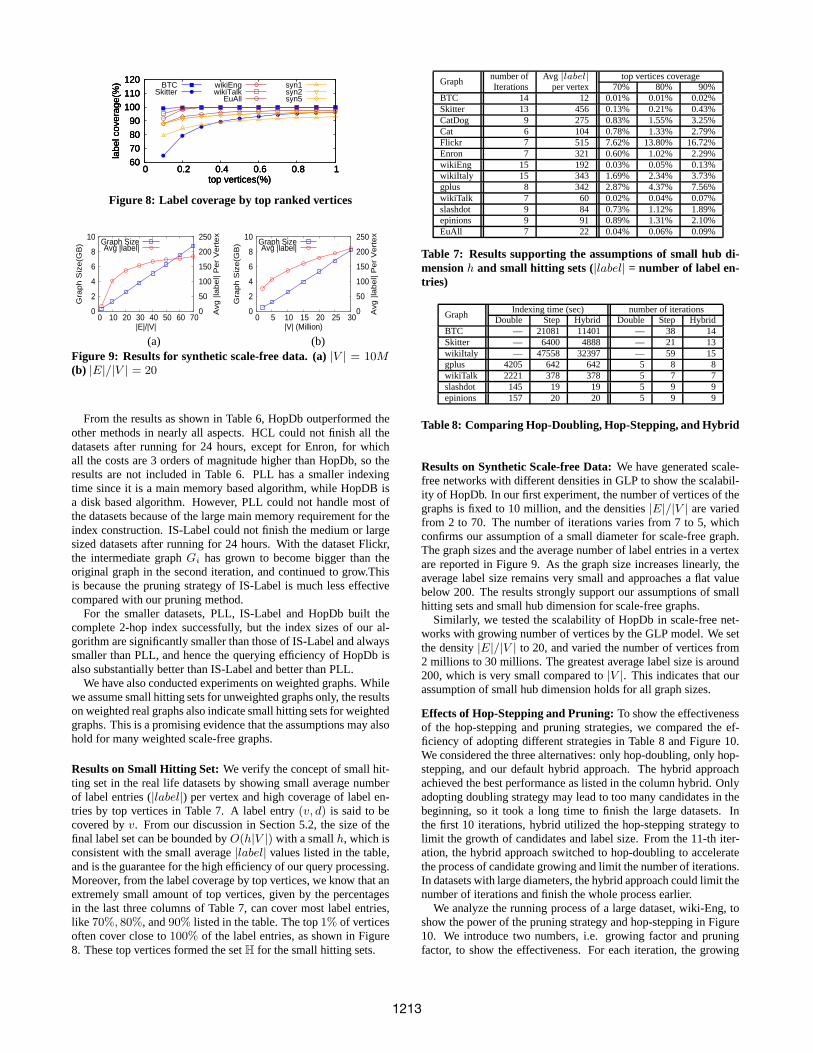
Results on Small Hitting Set:We verify the concept of small hit-ting set in the real life datasets by showing small average numberof label entries (|label|) per vertex and high coverage of label en-tries by top vertices in Table 7. A label entry(v, d) is said to becovered byv. From our discussion in Section 5.2, the size of thefinal label set can be bounded byO(h|V |) with a smallh, which isconsistent with the small average|label| values listed in the table,and is the guarantee for the high efficiency of our query processing.Moreover, from the label coverage by top vertices, we know that anextremely small amount of top vertices, given by the percentagesin the last three columns of Table 7, can cover most label entries,like 70%, 80%, and90% listed in the table. The top1% of verticesoften cover close to100% of the label entries, as shown in Figure8. These top vertices formed the setH for the small hitting sets.

Graphnumber of Avg |label| top vertices coverageIterations per vertex 70% 80% 90%

BTC 14 12 0.01% 0.01% 0.02%Skitter 13 456 0.13% 0.21% 0.43%CatDog 9 275 0.83% 1.55% 3.25%Cat 6 104 0.78% 1.33% 2.79%Flickr 7 515 7.62% 13.80% 16.72%Enron 7 321 0.60% 1.02% 2.29%wikiEng 15 192 0.03% 0.05% 0.13%wikiItaly 15 343 1.69% 2.34% 3.73%gplus 8 342 2.87% 4.37% 7.56%wikiTalk 7 60 0.02% 0.04% 0.07%slashdot 9 84 0.73% 1.12% 1.89%epinions 9 91 0.89% 1.31% 2.10%EuAll 7 22 0.04% 0.06% 0.09%

Table 7: Results supporting the assumptions of small hub di-mensionh and small hitting sets (|label| = number of label en-tries)

GraphIndexing time (sec) number of iterations

Double Step Hybrid Double Step HybridBTC — 21081 11401 — 38 14Skitter — 6400 4888 — 21 13wikiItaly — 47558 32397 — 59 15gplus 4205 642 642 5 8 8wikiTalk 2221 378 378 5 7 7slashdot 145 19 19 5 9 9epinions 157 20 20 5 9 9

Table 8: Comparing Hop-Doubling, Hop-Stepping, and Hybrid

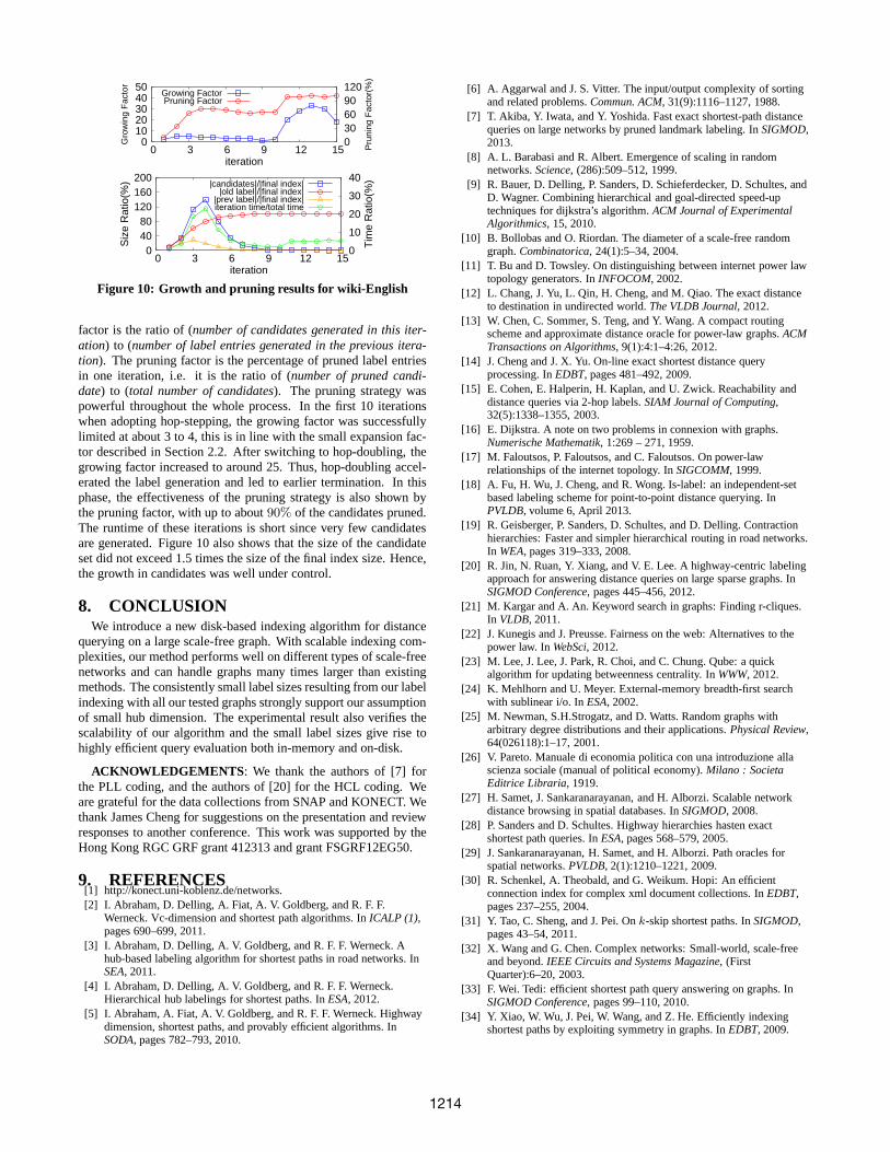
Results on Synthetic Scale-free Data:We have generated scale-free networks with different densities in GLP to show the scalabil-ity of HopDb. In our first experiment, the number of vertices of thegraphs is fixed to 10 million, and the densities|E|/|V | are variedfrom 2 to 70. The number of iterations varies from 7 to 5, whichconfirms our assumption of a small diameter for scale-free graph.The graph sizes and the average number of label entries in a vertexare reported in Figure 9. As the graph size increases linearly, theaverage label size remains very small and approaches a flat valuebelow 200. The results strongly support our assumptions of smallhitting sets and small hub dimension for scale-free graphs.

Similarly, we tested the scalability of HopDb in scale-freenet-works with growing number of vertices by the GLP model. We setthe density|E|/|V | to 20, and varied the number of vertices from2 millions to 30 millions. The greatest average label size isaround200, which is very small compared to|V |. This indicates that ourassumption of small hub dimension holds for all graph sizes.

Effects of Hop-Stepping and Pruning:To show the effectivenessof the hop-stepping and pruning strategies, we compared theef-ficiency of adopting different strategies in Table 8 and Figure 10.We considered the three alternatives: only hop-doubling, only hop-stepping, and our default hybrid approach. The hybrid approachachieved the best performance as listed in the column hybrid. Onlyadopting doubling strategy may lead to too many candidates in thebeginning, so it took a long time to finish the large datasets.Inthe first 10 iterations, hybrid utilized the hop-stepping strategy tolimit the growth of candidates and label size. From the 11-thiter-ation, the hybrid approach switched to hop-doubling to acceleratethe process of candidate growing and limit the number of iterations.In datasets with large diameters, the hybrid approach couldlimit thenumber of iterations and finish the whole process earlier.

We analyze the running process of a large dataset, wiki-Eng,toshow the power of the pruning strategy and hop-stepping in Figure10. We introduce two numbers, i.e. growing factor and pruningfactor, to show the effectiveness. For each iteration, the growing

1213

0 10 20 30 40 50

0 3 6 9 12 15 0 30 60 90 120

Gro

win

g F

acto

r

Pru

ning

Fac

tor(

%)

iteration

Growing FactorPruning Factor

0 40 80

120 160 200

0 3 6 9 12 15 0

10

20

30

40

Siz

e R

atio

(%)

Tim

e R

atio

(%)

iteration

|candidates|/|final index||old label|/|final index|

|prev label|/|final index|iteration time/total time

Figure 10: Growth and pruning results for wiki-English

factor is the ratio of (number of candidates generated in this iter-ation) to (number of label entries generated in the previous itera-tion). The pruning factor is the percentage of pruned label entriesin one iteration, i.e. it is the ratio of (number of pruned candi-date) to (total number of candidates). The pruning strategy waspowerful throughout the whole process. In the first 10 iterationswhen adopting hop-stepping, the growing factor was successfullylimited at about 3 to 4, this is in line with the small expansion fac-tor described in Section 2.2. After switching to hop-doubling, thegrowing factor increased to around 25. Thus, hop-doubling accel-erated the label generation and led to earlier termination.In thisphase, the effectiveness of the pruning strategy is also shown bythe pruning factor, with up to about90% of the candidates pruned.The runtime of these iterations is short since very few candidatesare generated. Figure 10 also shows that the size of the candidateset did not exceed 1.5 times the size of the final index size. Hence,the growth in candidates was well under control.

8. CONCLUSIONWe introduce a new disk-based indexing algorithm for distance

querying on a large scale-free graph. With scalable indexing com-plexities, our method performs well on different types of scale-freenetworks and can handle graphs many times larger than existingmethods. The consistently small label sizes resulting fromour labelindexing with all our tested graphs strongly support our assumptionof small hub dimension. The experimental result also verifies thescalability of our algorithm and the small label sizes give rise tohighly efficient query evaluation both in-memory and on-disk.

ACKNOWLEDGEMENTS : We thank the authors of [7] forthe PLL coding, and the authors of [20] for the HCL coding. Weare grateful for the data collections from SNAP and KONECT. Wethank James Cheng for suggestions on the presentation and reviewresponses to another conference. This work was supported bytheHong Kong RGC GRF grant 412313 and grant FSGRF12EG50.

9. REFERENCES[1] http://konect.uni-koblenz.de/networks.[2] I. Abraham, D. Delling, A. Fiat, A. V. Goldberg, and R. F. F.

Werneck. Vc-dimension and shortest path algorithms. InICALP (1),pages 690–699, 2011.

[3] I. Abraham, D. Delling, A. V. Goldberg, and R. F. F. Werneck. Ahub-based labeling algorithm for shortest paths in road networks. InSEA, 2011.

[4] I. Abraham, D. Delling, A. V. Goldberg, and R. F. F. Werneck.Hierarchical hub labelings for shortest paths. InESA, 2012.

[5] I. Abraham, A. Fiat, A. V. Goldberg, and R. F. F. Werneck. Highwaydimension, shortest paths, and provably efficient algorithms. InSODA, pages 782–793, 2010.

[6] A. Aggarwal and J. S. Vitter. The input/output complexity of sortingand related problems.Commun. ACM, 31(9):1116–1127, 1988.

[7] T. Akiba, Y. Iwata, and Y. Yoshida. Fast exact shortest-path distancequeries on large networks by pruned landmark labeling. InSIGMOD,2013.

[8] A. L. Barabasi and R. Albert. Emergence of scaling in randomnetworks.Science, (286):509–512, 1999.

[9] R. Bauer, D. Delling, P. Sanders, D. Schieferdecker, D. Schultes, andD. Wagner. Combining hierarchical and goal-directed speed-uptechniques for dijkstra’s algorithm.ACM Journal of ExperimentalAlgorithmics, 15, 2010.

[10] B. Bollobas and O. Riordan. The diameter of a scale-freerandomgraph.Combinatorica, 24(1):5–34, 2004.

[11] T. Bu and D. Towsley. On distinguishing between internet power lawtopology generators. InINFOCOM, 2002.

[12] L. Chang, J. Yu, L. Qin, H. Cheng, and M. Qiao. The exact distanceto destination in undirected world.The VLDB Journal, 2012.

[13] W. Chen, C. Sommer, S. Teng, and Y. Wang. A compact routingscheme and approximate distance oracle for power-law graphs.ACMTransactions on Algorithms, 9(1):4:1–4:26, 2012.

[14] J. Cheng and J. X. Yu. On-line exact shortest distance queryprocessing. InEDBT, pages 481–492, 2009.

[15] E. Cohen, E. Halperin, H. Kaplan, and U. Zwick. Reachability anddistance queries via 2-hop labels.SIAM Journal of Computing,32(5):1338–1355, 2003.

[16] E. Dijkstra. A note on two problems in connexion with graphs.Numerische Mathematik, 1:269 – 271, 1959.

[17] M. Faloutsos, P. Faloutsos, and C. Faloutsos. On power-lawrelationships of the internet topology. InSIGCOMM, 1999.

[18] A. Fu, H. Wu, J. Cheng, and R. Wong. Is-label: an independent-setbased labeling scheme for point-to-point distance querying. InPVLDB, volume 6, April 2013.

[19] R. Geisberger, P. Sanders, D. Schultes, and D. Delling.Contractionhierarchies: Faster and simpler hierarchical routing in road networks.In WEA, pages 319–333, 2008.

[20] R. Jin, N. Ruan, Y. Xiang, and V. E. Lee. A highway-centric labelingapproach for answering distance queries on large sparse graphs. InSIGMOD Conference, pages 445–456, 2012.

[21] M. Kargar and A. An. Keyword search in graphs: Finding r-cliques.In VLDB, 2011.

[22] J. Kunegis and J. Preusse. Fairness on the web: Alternatives to thepower law. InWebSci, 2012.

[23] M. Lee, J. Lee, J. Park, R. Choi, and C. Chung. Qube: a quickalgorithm for updating betweenness centrality. InWWW, 2012.

[24] K. Mehlhorn and U. Meyer. External-memory breadth-first searchwith sublinear i/o. InESA, 2002.

[25] M. Newman, S.H.Strogatz, and D. Watts. Random graphs witharbitrary degree distributions and their applications.Physical Review,64(026118):1–17, 2001.

[26] V. Pareto. Manuale di economia politica con una introduzione allascienza sociale (manual of political economy).Milano : SocietaEditrice Libraria, 1919.

[27] H. Samet, J. Sankaranarayanan, and H. Alborzi. Scalable networkdistance browsing in spatial databases. InSIGMOD, 2008.

[28] P. Sanders and D. Schultes. Highway hierarchies hastenexactshortest path queries. InESA, pages 568–579, 2005.

[29] J. Sankaranarayanan, H. Samet, and H. Alborzi. Path oracles forspatial networks.PVLDB, 2(1):1210–1221, 2009.

[30] R. Schenkel, A. Theobald, and G. Weikum. Hopi: An efficientconnection index for complex xml document collections. InEDBT,pages 237–255, 2004.

[31] Y. Tao, C. Sheng, and J. Pei. Onk-skip shortest paths. InSIGMOD,pages 43–54, 2011.

[32] X. Wang and G. Chen. Complex networks: Small-world, scale-freeand beyond.IEEE Circuits and Systems Magazine, (FirstQuarter):6–20, 2003.

[33] F. Wei. Tedi: efficient shortest path query answering ongraphs. InSIGMOD Conference, pages 99–110, 2010.

[34] Y. Xiao, W. Wu, J. Pei, W. Wang, and Z. He. Efficiently indexingshortest paths by exploiting symmetry in graphs. InEDBT, 2009.

1214