HONDO - t1.chem.umn.edut1.chem.umn.edu/hondoplus/HONDOPLUS_Manual_v5.2... · Restriction of orbital rotation based on dominant CSFs ... MCSCF Geometry Optimization ... algorithm for

HONDOPLUS

Users Manual

version 5.2

Date of Program Version: January 17, 2013

Date of Latest Manual Revision: January 20, 2013

H. Nakamura, J. D. Xidos, A. C. Chamberlin,

C. P. Kelly, R. Valero, K. R. Yang, J. D. Thompson,

J. Li, G. D. Hawkins, T. Zhu,

B. J. Lynch, Y. Volobuev, D. Rinaldi,

D. A. Liotard, C. J. Cramer, and D. G. Truhlar

including

HONDO 99

Users Manual

version 99.6

June 1999

M. Dupuis, A. Marquez, and E.R. Davidson

2

Table of Contents

Introduction to HONDOPLUS ................................................................................................................................................. 6 Major capabilities added in HONDOPLUS ............................................................................................................................. 6 Affiliations ............................................................................................................................................................................... 7 Acknowledgments .................................................................................................................................................................... 7 REQUIRED CITATIONS ........................................................................................................................................................ 8 Note about copyrights .............................................................................................................................................................. 8 What is new in HONDOPLUS–v5.2? ........................................................................................................................................... 8 What is new in HONDOPLUS–v5.1? ........................................................................................................................................... 9 What was new in HONDOPLUS–v5.0? ....................................................................................................................................... 9 What was new in HONDOPLUS–v4.9? ....................................................................................................................................... 9 What was new in HONDOPLUS–v4.8? ....................................................................................................................................... 9 What was new in HONDOPLUS–v4.7? ....................................................................................................................................... 9 What was new in HONDOPLUS–v4.6? ..................................................................................................................................... 10 What was new in HONDOPLUS–v4.5? ..................................................................................................................................... 10 What was new in HONDOPLUS–v4.4.1? .................................................................................................................................. 10 What was new in HONDOPLUS–v4.4? ..................................................................................................................................... 10 What was new in HONDOPLUS–v4.3? ..................................................................................................................................... 11 What was new in HONDO/S–v4.3? .......................................................................................................................................... 11 What was new in HONDO/S–v4.2? .......................................................................................................................................... 11 What was new in HONDO/S–v4.1? .......................................................................................................................................... 11 What was new in HONDO/S–v4.0? .......................................................................................................................................... 11 What was new in HONDO/S–v3.5? .......................................................................................................................................... 11 What was new in HONDO/S–v3.4.1? ....................................................................................................................................... 11 What was new in HONDO/S–v.3.4? ......................................................................................................................................... 12 What was new in HONDO/S–v.3.3? ......................................................................................................................................... 12 What was new in HONDO/S–v.3.2? ......................................................................................................................................... 12 What was new in HONDO/S–v.3.1? ......................................................................................................................................... 12 What was new in HONDO/S–v.3.0? ......................................................................................................................................... 13 What was new in HONDO/S–v.2.0? ......................................................................................................................................... 13 What was new in HONDO/S–v.1.0? ......................................................................................................................................... 13 What was new in HONDO–v.99.6? .......................................................................................................................................... 13 What was new in HONDO–v.95.6? .......................................................................................................................................... 13 What was new in HONDO–v.95.3? .......................................................................................................................................... 14 What was new in HONDO–v.8.5? ............................................................................................................................................ 14 What was new in HONDO–v.8.4? ............................................................................................................................................ 14 What was new in HONDO–v.8.3? ............................................................................................................................................ 15 HONDO Algorithms ................................................................................................................................................................. 16 Contents of the distribution package ...................................................................................................................................... 17 Installation .............................................................................................................................................................................. 22 Overview of HONDO ............................................................................................................................................................... 23

Capabilities ........................................................................................................................................................................ 23 Vectorization ..................................................................................................................................................................... 25 Parallelization .................................................................................................................................................................... 25 Memory management ........................................................................................................................................................ 25 Memory size requirements ................................................................................................................................................ 26 AIX, IRIX, and Linux implementations ............................................................................................................................ 26 Restart capabilities ............................................................................................................................................................. 27 The direct access file DA10 ............................................................................................................................................... 27 Input................................................................................................................................................................................... 27

Overview of HONDOPLUS........................................................................................................................................................ 28 Executive summary for the charge and solvation models.................................................................................................. 29

Löwdin population analysis and redistributed Löwdin population analysis ................................................................. 32 Charge Model 2, Charge Model 3, and Charge Model 4 .............................................................................................. 32 SMx (x = 5.42, 5.43, 6, and 6T) Solvation Models ....................................................................................................... 33

3

Analytical gradients and geometry optimizations .......................................................... Error! Bookmark not defined. Allowed Combinations of Solvent Model, Electronic Structure Theory, and Basis Set.................................................... 37

Notation ........................................................................................................................................................................ 39 SCRF calculations using generalized Born model and CM2, CM3, or CM4 charges .................................................. 40 Solvent-accessible surface area and solvation free energy in aqueous and organic solutions ...................................... 40

Literature references of the solvation models, charge models, electronic structure methods, and basis sets .................... 40 Usage of the solvation models ........................................................................................................................................... 47 The HONDOPLUS test suite of the charge and solvation models ......................................................................................... 50

Running the HONDOPLUS test suite ............................................................................................................................... 53 Verifying the correct installation of HONDOPLUS by using the test suite results ........................................................... 54

Description of the SM6 test suite ....................................................................................................................................... 55 Special notes on basis sets ................................................................................................................................................. 60 SCF schemes ..................................................................................................................................................................... 61 Density Functional Methods Recommended for use with CM4 and SM6 in HONDOPLUS ................................................ 63 Notation for the solvation models ...................................................................................................................................... 64 Executive summary for the diabatization method ............................................................................................................. 65 Theoretical background for diabatization .......................................................................................................................... 65 Usage for diabatization: How to calculate diabatic potentials with HONDOPLUS .............................................................. 67

Ordering of DMOs ........................................................................................................................................................ 67 Labeling of CSFs and dominant CSF group lists .......................................................................................................... 68 Determination of DMOs ............................................................................................................................................... 68 Symmetry of wave functions and DMOs ...................................................................................................................... 70 Restriction of orbital rotation based on dominant CSFs ............................................................................................... 70 Notes ............................................................................................................................................................................. 76

Test runs for the diabatization method .............................................................................................................................. 77 Platforms ........................................................................................................................................................................... 81 Further information ........................................................................................................................................................... 81 Acknowledgments ............................................................................................................................................................. 81 HONDOPLUS Revision History ............................................................................................................................................ 82

Data Group $JOB ............................................................................................................................................................... 91 Data Group $BAS ............................................................................................................................................................... 92 Data Group $GEO .............................................................................................................................................................. 96 Data Group $SYM .............................................................................................................................................................. 99 Namelist $CNTRL , $CTL .............................................................................................................................................. 100 Data group $BASIS .......................................................................................................................................................... 104 Namelist $OPT ................................................................................................................................................................ 112 Namelist $FREZ .............................................................................................................................................................. 114 Namelist $IRC ................................................................................................................................................................. 117 Namelist $FORCE ........................................................................................................................................................... 119 Namelist $MASS ............................................................................................................................................................. 121 Namelist $HSSINP .......................................................................................................................................................... 122 Data group $HESS............................................................................................................................................................ 123 Namelist $IRRAM ........................................................................................................................................................... 124 Data group $MUD ............................................................................................................................................................ 125 Data group $RAM ............................................................................................................................................................ 126 Namelist $NLO ............................................................................................................................................................... 127 Namelist $DYN ............................................................................................................................................................... 128 Namelist $PES ................................................................................................................................................................. 129 Data group $XYZ ............................................................................................................................................................. 130 Namelist $TRUDGE........................................................................................................................................................ 131 Namelist $GEXP ............................................................................................................................................................. 132 Namelist $SEAM ............................................................................................................................................................. 133 Namelist $ET ................................................................................................................................................................... 134 Namelist $ZMAT , $ZMT ............................................................................................................................................... 137 Namelist $GUESS ........................................................................................................................................................... 140 Data group $VEC ............................................................................................................................................................. 143

4

Data groups $VECA, $VECB ......................................................................................................................................... 144 Data groups $VECA-A, $VECB-A, $VECA-B, $VECB-B ............................................................................................ 145 Namelist $INTGRL ......................................................................................................................................................... 146 Namelist $WFN ............................................................................................................................................................... 148 Namelist $SCF................................................................................................................................................................. 149 Namelist $DFT ................................................................................................................................................................ 154 Namelist $CI .................................................................................................................................................................... 155 Namelist $MC ................................................................................................................................................................. 157 Namelist $ORD ............................................................................................................................................................... 161 Namelist $TRF ................................................................................................................................................................ 162 Data group $DRT ............................................................................................................................................................ 163 Namelist $GUGSRT ........................................................................................................................................................ 168 Namelist $GUGEM ......................................................................................................................................................... 169 Namelist $GUGDIA ........................................................................................................................................................ 170 Namelist $GUGDM ......................................................................................................................................................... 172 Namelist $GUGDM2 ....................................................................................................................................................... 173 Namelist $TRFDM2 ........................................................................................................................................................ 176 Namelist $CPHF .............................................................................................................................................................. 177 Namelist $MP2 ................................................................................................................................................................ 178 Namelist $MP4 ................................................................................................................................................................ 180 Namelist $CASMP2 ........................................................................................................................................................ 181 Namelist $MCQDPT ....................................................................................................................................................... 183 Namelist $PUN ................................................................................................................................................................ 186 Namelist $PRP................................................................................................................................................................. 188 Namelist $MLK ............................................................................................................................................................... 190 Namelist $GIAO .............................................................................................................................................................. 191 Namelist $DPL ................................................................................................................................................................ 192 Namelist $FPL ................................................................................................................................................................. 194 Namelist $SOS ................................................................................................................................................................ 197 Namelist $BOYS ............................................................................................................................................................. 198 Data group $STONE ........................................................................................................................................................ 199 Namelist $MAP , $GRID ................................................................................................................................................ 200 Namelist $FLD ................................................................................................................................................................ 202 Data group $QREL ........................................................................................................................................................... 203 Data group $EFC .............................................................................................................................................................. 204 Namelist $EFC2 .............................................................................................................................................................. 206 Data group $QMMM ........................................................................................................................................................ 207 Namelist $QM ................................................................................................................................................................. 208 Namelist $MMNOPOL ................................................................................................................................................... 209 Namelist $MMPOL ......................................................................................................................................................... 210 Namelist $ZRF ................................................................................................................................................................ 211 Namelists $HONDOS, $CM2, and $SM5 ............................................................................................................................ 212

HONDOPLUS Keywords Required for Running Standard SMx Calculations ............................................................... 218 Namelist $COSMO ......................................................................................................................................................... 219 Data group $ECP ............................................................................................................................................................. 220 Namelist $CSOV ............................................................................................................................................................. 222 Namelist $BSSE .............................................................................................................................................................. 223 Namelist $DIABAT ......................................................................................................................................................... 224 Namelist $PROTOTYPE ................................................................................................................................................. 227 Data group $DIAVEC ..................................................................................................................................................... 228 Data group $DFMVEC ....................................................................................................................................................... 229 Data group $CSFDAT ......................................................................................................................................................... 230 File directory for DA10 ........................................................................................................................................................ 232 How to read the tape on AIX/RS6000 .................................................................................................................................. 236 How to run HONDOPLUS ....................................................................................................................................................... 237 Namelist $FIL .................................................................................................................................................................. 238

5

How to compile and Run the POE parallel version of HONDO ............................................................................................. 240 Namelist $PVM ............................................................................................................................................................... 241 SAMPLE 1: SCF Geometry Optimization ....................................................................................................................... 242 SAMPLE 2: MCSCF Geometry Optimization ................................................................................................................. 243 SAMPLE 3: SCF Force constant calculation ................................................................................................................... 244 SAMPLE 4: Property Calculation .................................................................................................................................... 245 SAMPLE 5: CI calculation ............................................................................................................................................... 246 SAMPLE 6: MP2 calculation ........................................................................................................................................... 248 SAMPLE 7: MP4 calculation ........................................................................................................................................... 249 SAMPLE 8: ECP Calculation ........................................................................................................................................... 250 SAMPLE 9: MIXED BASIS SET calculation ................................................................................................................. 252 SAMPLE 10: GENERAL BASIS SET calculation .......................................................................................................... 253 SAMPLE 11: MP2 Geometry Optimization ..................................................................................................................... 254 SAMPLE 12: MP2 Finite Difference Force Constant calculation .................................................................................... 255 SAMPLE 13: MP2 Geometry Optimization ..................................................................................................................... 256 SAMPLE 14: RHF Analytical Force Constant Calculation.............................................................................................. 257 SAMPLE 15: RHF Analytical Force Constant Calculation.............................................................................................. 258 SAMPLE 16: First Order CASSCF Calculation ............................................................................................................... 259 SAMPLE 17: Frequency-dependent (hyper)polarizability calculation ............................................................................. 261 SAMPLE 18: Electron Transfer Coupling Matrix Element calculation ........................................................................... 262 SAMPLE 19: CAS-MP2 calculation ................................................................................................................................ 263 SAMPLE 20: MC-QDPT2 calculation ............................................................................................................................. 264 SAMPLE 21: MC-QDPT2 calculation ........................................................................................................................... 267 SAMPLE 21-1: MC-QDPT2 calculation of SAMPLE 21 with EDSHFT=0.02 (ISA method) ...................................... 269 SAMPLE 22: Molecular Dynamics calculation ............................................................................................................... 271 SAMPLE 23: CSOV calculation ...................................................................................................................................... 272 SAMPLE 24: DFT(B3LYP) calculation........................................................................................................................... 274 SAMPLE 25: Finite-Field 2D NLO calculation ............................................................................................................... 275 SAMPLE 26: QM/MM (MD) calculation of water dimer ................................................................................................ 276 SAMPLE 26-1: QM/MM (MD) calculation of water dimer with a non-polarizable solvent (water) .............................. 277 SAMPLE 27: COSMO calculation---DISCONTINUED ................................................................................................ 278 SAMPLE 28: HF/6-31G(d) optimization of water with the H-O-H angle frozen .......................................................... 278 SAMPLE S1: SM6/mPW1PW91/MIDI!6D single-point calculation of water dimer in water. ....................................... 279 SAMPLE S2: SM6/B3LYP/6-31G* geometry optimization of water in water ................................................................ 280 SAMPLE S3: SM5.43/HF/6-31G* liquid-phase gradient calculation for HF in ethyl acetate ......................................... 281 SAMPLE S4 Diabatization of HNCO(S0,S1) based on CASSCF (Threefold density criterion) ......................................... 282 SAMPLE S5 Diabatization of HNCO(S0,S1) based on CASSCF (Fourfold way with one reference MO) ........................ 285 SAMPLE S6 Diabatization of HNCO(S0,S1) based on CASSCF ....................................................................................... 286 SAMPLE S7 Diabatization of HNCO(S0,S1) based on MC-QDPT .................................................................................... 287 SAMPLE S8 Diabatization of NH3(S0,S1) based on CASSCF (Threefold density criterion) ............................................. 292 SAMPLE S9 Diabatization of NH3(S0,S1) based on MC-QDPT with ISA method ............................................................ 295 SAMPLE S10 Diabatization of BrCH2C(O)Cl (S1, S2, S3, S4, S5, S6) based on CASSCF (Threefold density criterion) . 296 SAMPLE S11 Diabatization of BrCH2C(O)Cl (S1, S2, S3, S4, S5, S6) based on CASSCF (Fourfold way) ...................... 301

6

Introduction to HONDOPLUS

HONDOPLUS is a modified version of the HONDO-v99.6 electronic structure program. HONDOPLUS began as

HONDO/S, with solvation methods added to HONDO. As additional capabilities were added, not related to solvation, the

name was changed to HONDOPLUS.

As compared to HONDO, the HONDOPLUS program has enhancements in the following areas:

• Major new capabilities

• diabatization

• solvation

• new methods for calculating partial atomic charges

• intruder state avoidance in MRMP2 and MC-QDPT

• Other enhancements

• additional basis sets

• user-defined density functionals

• improved portability

• improved manual

• more complete test suites.

A list of capabilities of HONDO is given in the "Overview of HONDO" section of the manual. The enhancements in

HONDOPLUS are summarized above and are described in detail in the revision summaries in the "What's New" sections of

the manual. The major new capabilities are summarized next:

Major capabilities added in HONDOPLUS

• Diabatization

The fourfold way is a method of diabatization of coupled electronic states based on defining diabatic molecular orbitals

(DMOs), re-expressing CASSCF or MC-QDPT wave functions in terms of DMOs, and transforming to diabatic

configuration state functions by configurational uniformity. The diabatic states span the same space as N adiabatic states,

which may be the N lowest-energy adiabatic states, or the ground state may be excluded. There are three options:

• diabatize CASSCF wave functions based on state-averaged CASSCF DMOs

• diabatize MC-QDPT wave functions based on MC-QDPT DMOs

• diabatize MC-QDPT wave functions based on state-averaged CASSCF DMOs.

The program also computes the diagonal and off-diagonal elements of the diabatic potential energy matrix.

References for diabatization:

H. Nakamura and D. G. Truhlar, J. Chem. Phys. 115, 10353 (2001), 117, 5576 (2002), 118, 6816 (2003). K. R. Yang, X.

Xu, and D. G. Truhlar, Chem. Phys. Lett., submitted.

• Solvation

HONDOPLUS includes:

• the analytic surface area (ASA) algorithm for solvent-accessible surface areas and their gradients

• the generalized Born approximation (GBA) for implicit-solvent calculations of free energies of solvation

• the following universal generalized Born solvation models:

• SM5.42R and SM5.42

• SM5.43R and SM5.43

• SM6

• SM6T

7

Universal solvation models may be applied to almost any solvent.

References for solvation capabilities:

ASA D. A. Liotard, G. D. Hawkins, G. C. Lynch, C. J. Cramer, and D. G. Truhlar, J. Comp. Chem. 16, 422 (1995).

GBA C. J. Cramer and D. G. Truhlar, J. Am. Chem. Soc. 113, 8305 (1991).

SM5.42 T. Zhu, J. Li, G. D. Hawkins, C. J. Cramer, and D. G. Truhlar, J. Chem. Phys. 109, 9117 (1998).

SM5.43 J. D. Thompson, C. J. Cramer, and D. G. Truhlar, Journal of Physical Chemistry A 108, 6532-6542 (2004).

SM6 C. P. Kelly, C. J. Cramer, and D. G. Truhlar, J. Chem. Theory Comput. 1, 1133 (2005).

SM6T A. C. Chamberlin, C. J. Cramer, and D. G. Truhlar, J. Phys. Chem. B 110, 5665 (2006).

• Charge analysis

HONDOPLUS includes the following additional methods for charge analysis:

• Löwdin population analysis (LPA)

• redistributed Löwdin population analysis (RLPA)

• the following class IV charge models

• charge model 2 (CM2)



References for these methods:

LPA P. O. Löwdin, Phys. Rev. 97, 1474 (1955). J. Baker, Theor. Chim. Acta 68, 221 (1985).

RLPA J. D. Thompson, J. D. Xidos, T. M. Sonbuchner, C. J. Cramer, and D. G. Truhlar, PhysChemComm 5, 117

(2002).

CM2 J. Li, T. Zhu, C. J. Cramer, and D. G. Truhlar, J. Phys. Chem. A 102, 1820 (1998).

CM3 P. Winget, J. D. Thompson, J. D. Xidos, C. J. Cramer, and D. G. Truhlar, J. Phys. Chem. A 106, 10707 (2002).

CM4 C. P. Kelly, C. J. Cramer, and D. G. Truhlar, J. Theor. Comput. Chem, 1, 1133 (2005).

• Intruder state avoidance

The intruder state avoidance (ISA) method of H.A. Witek, Y.-K. Choe, J.P. Finley, and K. Hirao, J. Comput. Chem. 10,

957 (2002) has been implemented. The starting code for the modification was taken from the GAMESS program with

permission from Professor Mark Gordon, Ames Laboratory, Iowa State University.

Affiliations

M. Dupuis, Pacific Northwest National Laboratory, EMSL, K8-91, P.O.Box 999, Richland WA 99352, USA.

A. Marquez, Department of Chemistry, University of Sevilla, Sevilla, Spain.

E.R. Davidson, Department of Chemistry, Indiana University, Bloomington IN 47405, USA.

H. Nakamura, J.D. Xidos, C.P. Kelly, R. Valero, K.R. Yang, J.D. Thompson, B.J. Lynch, J. Li, G.D. Hawkins, T. Zhu, Y.

Volobuev, C.J. Cramer and D.G. Truhlar, Department of Chemistry and Supercomputer Institute, University of

Minnesota, Minneapolis MN 55455-0431, USA.

D. Rinaldi, Laboratoire de Chimie Theoriqe, Universite de Nancy, I, Vandoeuvre-Nancy 54506, France.

D.A. Liotard, Laboratoire de Physico-Chimie Theorique, Universite de Bordeaux 1, 33405 Talence, France.

Acknowledgments

The HONDO program originated in the group of Harry F. King as part of the Ph.D. research of Michel Dupuis and John Rys.

The development of the program has subsequently been led by Michel Dupuis. Antonio Marquez (University of Sevilla)

8

and Ernest R. Davidson (University of Indiana) have provided much code and many ideas. Recent contributions are due to:

M. Klobukowski (University of Alberta), K. Hirao, T. Nakajima, K. Nakayama, Y. Kawashima, and H. Nakano (University

of Tokyo); M. Aida (Hiroshima University); D.G. Truhlar, C.J. Cramer, H. Nakamura, J.D. Xidos, J.D. Thompson, C.P.

Kelly, R. Valero, B.J. Lynch, Y. Volobuev, J. Li, and G.D. Hawkins (University of Minnesota); Dr. D.A. Liotard

(Universite de Bordeaux 1), and D. Rinaldi (Universite de Nancy). Earlier contributions were due to: M.S. Gordon and Dr.

M. Schmidt and their group (Iowa State University), J.P. Flament, P.M. Kozlowski, F. Johnston, S. Chin, E. Hollauer, S.

Maluendes, A. Farazdel, S. Karna, P. Mougenot, C. Daniel, J.D. Watts, G.J.B. Hurst, H.O. Villar, W. Stevens, H. Basch, S.

Elbert, B. Liu, K. Dyall, R. Lindh, T. Takada, B. Brooks, W. Laidig, P. Saxe, D. Spangler, and J. Wendoloski.

REQUIRED CITATIONS

Any publication based upon results obtained with this program should include the following citations:

HONDOPLUS–v.5.2, by H. Nakamura, J.D. Xidos, A.C. Chamberlin, C.P. Kelly, R. Valero, K. R. Yang, J.D.

Thompson, J. Li, G.D. Hawkins, T. Zhu, B.J. Lynch, Y. Volobuev, D. Rinaldi, D.A. Liotard, C.J. Cramer, and D.G.

Truhlar, University of Minnesota, Minneapolis, 2013, based on HONDO–v.99.6.

M. Dupuis, A. Marquez, and E.R. Davidson, “HONDO 99.6”, 1999, based on HONDO 95.3, M. Dupuis, A. Marquez,

and E.R. Davidson, Quantum Chemistry Program Exchange (QCPE), Indiana University, Bloomington, In 47405.

Any publication based upon results obtained with the CAS-MP2 program must include the following citation:

P.M. Kozlowski and E.R. Davidson, J. Chem. Phys. 100, 3672 (1994).

Note about copyrights

The original code up to HONDO 8.2 was not copyrighted. The HONDO 95.6 code is copyrighted to IBM Corporation. A

license for the code can be obtained from the Quantum Chemistry Program Exchange, Indiana University. The

enhancements to HONDO 99 are contributions from some of the developers listed above.

The SMx (x = 5.42, 5.43, or 6) solvation models, CM2, CM3, and CM4 charge models, the diabatic states algorithms, and

the corresponding additions to the code and the manual are copyrighted as part of the Minnesota Charge and Solvation

Technology and are included in HONDO 99 under a special understanding between the HONDO developers and the solvation

model and charge model developers. The subroutines remain copyrighted to the authors and their institution. For further

information about the solvation and charge model enhancements, contact Professor Christopher J. Cramer and Professor

Donald G. Truhlar, Department of Chemistry, University of Minnesota, and for further information about the diabatic states

enhancements, contact Professor Donald G. Truhlar, Department of Chemistry, University of Minnesota. Other

enhancements to HONDOPLUS, in particular the mPW code and the diabatization code are also copyrighted and included in

HONDO 99 under special understanding between the HONDO developers and the HONDOPLUS coauthors. The subroutines

remain copyrighted to the authors and their institutions. For further information contact Professor Donald G. Truhlar,

Department of Chemistry, University of Minnesota.

What is new in HONDOPLUS–v5.2?

A new scheme has been added to the fourfold way diabatization of MC-QDPT wave functions with CASSCF DMOs. See

"Direct Diabatization of Electronic States by the Fourfold Way: Including Dynamical Correlation by Multi-Configuration

Quasidegenerate Perturbation Theory with Complete Active Space Self-Consistent-Field Diabatic Molecular Orbitals," K.R.

Yang, X. Xu, and D.G. Truhlar, Chem. Phys. Lett., submitted.

9

What is new in HONDOPLUS–v5.1?

The intruder state avoidance (ISA) method has been implemented. See H.A. Witek, Y.-K. Choe, J.P. Finley, and K. Hirao,

J. Comput. Chem. 10 957 (2002). The original code has been taken from the GAMESS program with permission from

Professor Mark Gordon, Ames Laboratory, Iowa State University. The ISA method is useful in MRMP2 (single-state)

and MCQDPT (multi-state) multireference perturbative calculations whenever so-called “intruder states” are present.

Intruder states cause the energy denominators in some terms of the perturbation expansion to be close to zero. To avoid

unphysically large contributions of those terms to the energy, in the ISA method each denominator x is replaced by x +

EDSHFT/x. This change only has an important effect on small x values, whereas for large x the effect of such change is

small. A new keyword EDSHFT has been added to the $MCQDPT namelist. The recommended value of EDSHFT is

0.02 2h

E (where Eh denoes a hartree), although some experimentation might be required for a particular system in

order to produce smooth potential energy surfaces. Note that only the non-relativistic part (i.e., without spin-orbit

terms) of the ISA method as implemented in GAMESS has been introduced into HONDOPLUS-v5.1.

A new capability has been added to the fourfold way diabatization procedure. In previous versions of HONDOPLUS, when

using the fourfold way all the N adiabatic states included in a CASSCF or MCQDPT calculation had to be transformed

to the diabatic representation. In HONDOPLUS-v5.1, an option is added to exclude the ground state from the fourfold

way procedure. In this case, only the N 1 excited adiabatic states and energies are transformed to the diabatic

representation. The keyword NGRSTATE has been added to the $DIABAT namelist to allow the user to run fourfold

way calculations with or without the ground state included.

The fourfold way now runs on non-IBM as well as IBM machines. The list of machines tested includes IBM Power 4

Regatta, Netfinity (Redhat Linux, pgf77 compiler), SGI Altix (Redhat Linux), and SunBlade 2000 (Solaris 9).

What was new in HONDOPLUS–v5.0?

A new method, SM6T, has been implemented. The model can be used to compute aqueous free energies of solvation as a

function of temperature over the temperature range 273-373 K. This involved modification of both the bulk-

electrostatic contributions,GENP, and the non-bulk electrostatic contributions, GCDS. Three new keywords SolK,

ReadK, and AvgK are now available.

SolK computes the free energy of solvation at the temperature specified

ReadK computes free energies of solvation for a list if temperatures provided in a file

AvgK computes free energies of solvation for a list of temperature provided in a file, but computes the

electrostatic portion by computing GENP for the average of all the temperatures in the file and then

using a scaling factor to compute GENP for the individual temperatures


A number of refinements to the code have been made in order to make HONDOPLUS compatible with the gnu g77 compiler.

With this compatibility, HONDOPLUS can now installed on more platforms than previous versions (e.g., SGI Altix, Mac

G5).


For methods that use diffuse basis functions, ISCRF=1 (SCF Scheme I) is no longer available due to convergence

problems.

An extended test suite for SM6 has been added. The input and output files for this portion of the test suite are located under

the directory /sm6.


10

The parameters sets for CM3/HF/MIDI! and CM3.1/HF/MIDI! have been added. CM3.1 is designed to give accurate

charges for high-energy materials.

The parameters sets for CM4/DFT/MIDI!6D, CM4/DFT/6-31G(d), CM4/DFT/6-31+G(d), and CM4/DFT/6-31+G(d,p),

where DFT is any good density functional, have been added.

The parameters sets for SM6/DFT/MIDI!6D, SM6/DFT/6-31G(d), SM6/DFT/6-31+G(d), and SM6/DFT/6-31+G(d,p) have

been added.

The section entitled “Density Functional Methods Recommended for use with CM4 and SM6 in HONDOPLUS–v4.7” has been

added. This section gives a description of the density functionals available in HONDOPLUS–v4.7 that are recommended

for use with CM4 and SM6.

The keywords IRADII and ISTS was added. The IRADII keyword specifies the set of atomic-number-dependent radii that

are used to build the molecular cavity. The ISTS keyword determines whether SM5- or SM6-type functionals are

used.

Coulomb radii are now defined for all atoms on the periodic table. In previous versions, atoms whose Coulomb radii were

not optimized as part of a given solvent model were assigned default values of 0 Å for the SCRF portion of the

solvation calculation. In HONDOPLUS–v4.7, atoms whose Coulomb radii have not been optimized are assigned a radius

equal to Bondi’s value for the van der Waal’s radius. Atoms for which Bondi has not assigned atomic radii to are

assigned a value of 2.0 Å. Thus, Generalized Born calculations can be carried out for molecules containing any

element on the periodic table.

The keyword SolvRd was added. This keyword allows the user to specify a value for the solvent radius, which is used for

the calculation of the solvent-accessible surface areas of the atoms of the solute.

The “R” notation used by SM5.42 and SM5.43 to distinguish single-point solvation calculations based on rigid gas-phase

geometries from liquid-phase geometry optimizations has been dropped for all models. The Pople style notation (i.e.

level/basis//level/basis) is now used.


The parameters sets for SM5.43R (which may also be used for SM5.43) with the MPWX/MIDI!, MPWX/MIDI!6D,

MPWX/6-31G(d), MPWX/6-31+G(d), and MPWX/6-31+G(d,p) with X = 0 – 60.6. The MPWX method uses Barone

and Adamo’s modified version of Perdew and Wang’s exchange functional, Perdew and Wang’s PW91 correlation

functional, and a percentage X of Hartree-Fock exchange. The SM5.43R parameters are defined for any value of X

between 0 and 60.6. These methods can be used for the calculation of the free energy of solvation. They can also be

used to carry out geometry optimizations with analytic free energy gradients in the liquid phase, liquid-phase numerical

Hessian calculations based on analytical free energy gradients, and potential of mean force calculations.


The parameters sets for SM5.43R (which may also be used for SM5.43) with the HF/6-31G(d), B3LYP/6-31G(d),

mPW1PW91/6-31G(d), and mPW1PW91/6-31+G(d) methods have been added. These methods can be used for the

calculation of the free energy of solvation. They can also be used to carry out geometry optimizations with analytic

free energy gradients in the liquid phase, liquid-phase numerical Hessian calculations based on analytical free energy

gradients, and potential of mean force calculations.

What was new in HONDOPLUS–v4.4.1?

A bug that affected liquid-phase geometry optimizations for systems larger than 15 atoms was fixed.


The program can now run on workstations running the RedHat Linux operating system.

11


The name of the program changed.

What was new in HONDO/S–v4.3?

The algorithm of diabatization, called the “fourfold way”, was improved by introducing the “pre-fourfold way” procedure.


The Charge Model (CM3) parameters for the BLYP/6-31G*, B3LYP/MIDI!6D, B3LYP/6-31G*, and B3LYP/6-31+G*

methods were implemented. Both gas-phase and liquid-phase CM3 charges can be calculated for these methods. This

charges can be used for generalized Born (GB) calculations of the electrostatic contribution to the free energy of

solvation. In addition, the corresponding free energy gradient can be calculated and used in geometry optimizations.

The test suite was extended to test the new CM3 parameter sets implemented in this version of the code.


The Charge Model 3 (CM3) parameters, which allow for evaluation of CM3 charges, were added. Both gas-phase and

liquid-phase CM3 charges and the electrostatic contribution to the free energy of solvation using the generalized Born

(GB) model can be calculated. In addition, CM3/GB analytical gradients may also be evaluated and used for geometry

optimizations

The redistributed Löwdin population analysis (RLPA) method was implemented. This new method can be used to evaluate

gas-phase and liquid-phase RLPA charges. The RLPA charges can further be used in a calculation of the electrostatic

contribution to the free energy of solvation using the generalized Born model and in a calculation of the corresponding

free energy gradient, which can also be used for geometry optimizations.

The namelist that controls Löwdin, RLPA, Charge Models 2 and 3, and SM5.42 solvation model specifications has been

broadened to support the new options (options pertaining to CM3 and RLPA) as well as the previous ones. This

namelist is now called $HONDOS (although the old names, $CM2 and $SM5, may also be used if desired). To

accommodate the CM3 Charge Model and the RLPA method, the allowed values of the ICMD keyword have been

extended to include 300, 302, 303, and 315 – 319. Also, the HFE keyword, which specifies the percentage of HF

exchange used in the mPW exchange functional for CM3 calculations, has been added.

The test suite was extended to test all of the CM3 parameter sets and to test the use of RLPA charges.

The MG3 and MG3S basis sets are now stored internally in the HONDOPLUS code. The keywords, MG3 and MG3S were

added to $BAS to request these new internally stored basis sets.


The algorithm to calculate diabatic states based on configurational uniformity was implemented.


All Fortran 90 code, which was introduced in version 3.2, has been removed. This modification was made in an effort to

make HONDO/S a more portable code.

What was new in HONDO/S–v3.4.1?

12

Corrections to the SM5.42 parameters for silicon have been implemented, and the sample calculations have been updated.

For details of the parameters and the parameterizations, refer to “Parameterization of a Universal Solvation Model for

Molecules Containing Silicon”; Winget, P; Thompson, J. D., Cramer, C. J.; Truhlar, D. G. J. Phys. Chem. B 2002, 106,

5160.

What was new in HONDO/S–v.3.4?

The MIDIX basis set (also known as MIDI!) is now stored internally. It can be requested with the MIDIX keyword in the

$BAS or $BASIS data groups. Examples of the new keyword are given for test suite cases that use the MIDIX basis

set.

The 6-31G and 6-31G* basis sets for third row atoms have been added.

Two versions of the 6-31G and 6-31G* basis sets for Si and the third row are now available. See the section entitled

Special notes on basis sets for further details. Test suite calculations for potassium, scandium, and bromine have been

added.

The SM5.42 parameters for silicon have been implemented, and sample calculations employing these parameters have been

added to the test suite.

PERL scripts for data collection from a large portion of the test suite output have been added for quick and easy checking

that the program has been installed correctly.


HONDO is now compatible with SGI platforms running IRIX operating systems as well as with IBM platforms

running AIX.

New namelist names for $OPTZ (now called $FREZ) and $MM (now called $MMNOPOL) are now used to avoid

portability problems.

User-defined density functionals for energy and analytic gradient calculations have been added.

The test suite was extended to illustrate the use of the new namelist names and to illustrate the new user defined

density functionals.


CM2 partial atomic charge and SM5.42R solvation model calculations are available for unrestricted wave functions;

SM5.42 solvation model calculations with analytical gradients are available for unrestricted wave functions that

employ Cartesian basis functions.

CM2 partial atomic charge and SM5.42R solvation model calculations for BPW91 wave functions; SM5.42/BPW91

solvation model calculations with analytical gradients are available for basis sets that employ Cartesian basis functions

(i.e., MIDI!6D, 6-31G*, and DZVP).

Generalized Born (GB) solvation model energy calculations using Löwdin charges are enabled. Analytical gradients

are available for wave functions that employ Cartesian basis functions.

Löwdin charge, CM2 charge, SM5.42R, SM5.42, and GB calculations for wave functions that employ spherical

harmonic f functions.

The DZVP basis set for H, C, N, O,F, Si, P, S, Cl, Br, and I is provided in file dzvp.bas.

New test cases in the test suite that perform CM2/BPW91, SM5.42R/BPW91, SM5.42R/UHF, and Generalized Born

(GB) calculations


Energies and analytical gradients for BPW91, mPW1PW91, and MPW1K density functionals.

Extended test suite to include geometry optimizations using each of the three new methods.

13


Analytical gradients and geometry optimizations (local minima only) for SM5.42/RHF/MIDI!6D,

SM5.42/RHF/6-31G*, and SM5.42/RHF/6-31+G*.

Single point gradient calculations can be requested for cases where analytical gradients are available.

A larger test suite that includes gradient evaluations for SM5.42/RHF/MIDI!6D and SM5.42/RHF/6-31G*, and the

geometry optimization of 2,4-pentadione in acetonitrile solution.


Löwdin atomic charges for wave functions that use spherical harmonic d functions.

CM2 partial atomic charges for HF/MIDI!, B3LYP/MIDI!, and HF/cc-pVDZ.

SM5.42R free energies of solvation for HF/MIDI!, B3LYP/MIDI!, and HF/cc-pVDZ.

New test suite.

Improved manual.


Löwdin atomic charges for wave functions that use Cartesian basis functions.

CM2 partial atomic charges for HF/MIDI!6D, HF/6-31G*, and HF/6-31+G*.

SM5.42R free energies of solvation for HF/MIDI!6D, HF/6-31G*, and HF/6-31+G*.

What was new in HONDO–v.99.6?

Molecular Dynamics driver for all wave functions and energies.

DFT and U-DFT capabilities (standard with disk, serial and parallel) with LDA, SLYP, BLYP, and B3LYP functionals

DFT and U-DFT analytic gradients

QM/MM model of solute/water systems with 3-site models of water (TIP3P, POL1, POL2, …), including polarizable

potentials and intra-molecular vibrational potential, for HF, MCSCF, and DFT wave functions.

QM/MM analytic gradient for the above potentials

COSMO continuum model for HF, MCSCF, and DFT wave functions.

Truhlar-Cramer SM5.42R continuum model (energy only) for HF and DFT

GIAO chemical shifts for SCF wave function (serial and parallel)

CSOV fragment analysis

Eigenvector Following method for transition-state search

Potential-derived charges

Option to do 22 orbital rotations of the initial guess orbitals

Relativistic one-electron Darwin and Mass-Velocity terms treated in the SCF, CASSCF, DFT….

Calculate Cartesian gradients by finite difference when analytic gradients are not available

Calculate Cartesian second derivate matrix by finite difference of the energy when analytic gradients and analytic hessian

are not available

Details can be found in appropriate sections of this documentation.


14

Easy definition of LST in internal coordinates using Z-matrix input.



Change in the name numbering for ease of maintenance: The name is now based on the year and the month.

Standard, semi-direct, direct Restricted Open Shell MP2 energy calculation (ROHF-MP2).

Allow up to 30 primitive Gaussian functions in any given contracted shell.

Improved disk space utilization for storing the electron repulsion integrals on file FT08 and FT09 by means of the THIZE

and MBYTES parameters in $INTGRL.

Definition of alternate files where initial vectors and hessian matrices can be found. See parameters GSSFIL, HSSFIL, and

FORFIL in namelists $GUESS, $OPT, $SAD, $IRC, and $FORCE for details.

Capability for reading the '.car’ file created from Biosym's INSIGHT graphical interface. See the parameter GEOFIL in the

namelist $BASINP for details.

Creation of a '.car' compatible file at the end of a run. Also a skeleton input file for the GAMESS code gets created.



Onsager's reaction field model for RHF, UHF, GVB energies and gradients.

Onsager's reaction field model for RHF in connection with NLO calculations, analytically or via finite field approach, for

static or frequency-dependent field.

Initial version of CAS-MP2 code from Prof. E.R. Davidson's group.

Parallel standard, direct, semi-direct algorithm for first-order convergent CAS calculations.

Improved default for initial guess orbitals.

Easy flagging of 'ghost' atoms in $BAS, $GEO, and $BASIS .

Code optimization in selected modules.

Definition of the $MLK to control Mulliken's population analysis.

Population analysis in the spherical harmonics basis, if requested.



Key word oriented input with Z-matrix compatibility.

Initial guess by concatenation of fragment molecular orbitals.

Direct and semi-direct algorithms for CAS, MCSCF, MP2 and UMP2 energies, and MP2 gradients, and for RHF analytical

second derivatives calculations.

Direct and semi-direct algorithms for ROHF and GVB.

Direct and semi-direct algorithms for static hyperpolarizabilities.

Direct and semi-direct algorithms for dynamic hyperpolarizabilities.

Parallel algorithms for RHF, UHF, ROHF, and GVB energies and gradients.

Parallel algorithms for standard closed shell MP2 energy calculation.

Parallel direct algorithms for RHF, UHF, ROHF, and GVB.

Parallel semi-direct algorithms for RHF, UHF, ROHF, and GVB.

15

Parallel standard, direct and semi-direct algorithms for static hyperpolarizabilities.

Parallel standard, direct and semi-direct algorithms for dynamic hyperpolarizabilities.

Sum-over-states (hyper)polarizability calculations.

Stone's distributed multipole analysis.

Automatic determination of orbital symmetry in $DRT input.

Tabulation of the compact effective core potentials and associated basis sets for all atoms up to Z=86, except the

lanthanides.

Key words for 6-31G**, 6-31G*, 6-31G, 4-31G**, 4-31G*, 4-31G, 3-21G**, 3-21G*, and 3-21G basis sets in $BASIS.



Capability for calculation of analytical MP2 energy gradient, for closed-shell HF wave function.

First-Order CAS wave function calculation to allow larger basis sets in MCSCF.

Semi-direct closed shell HF and UHF calculations.

Option for using spherical harmonics basis functions only.

Option for using more than 255 basis functions for HF, UHF, ROHF, GVB wave functions.

In-memory algorithms for HF, UHF, ROHF, GVB, and MP2, and MP2-gradient.

Improved HF second derivatives, MCSCF, MP4.

Thermochemical data after vibrational analysis.

Symmetry analysis of normal modes of vibration.

Free-input format to replace fixed-format input.


16

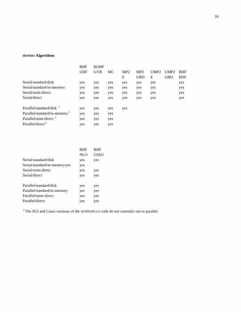
HONDO Algorithms

RHF ROHF

UHF GVB MC MP2 MP2 UMP2 UMP2 RHF

E GRD E GRD HSS

Serial/standard/disk yes yes yes yes yes yes yes

Serial/standard/in-memory yes yes yes yes yes yes yes

Serial/semi-direct yes yes yes yes yes yes yes

Serial/direct yes yes yes yes yes yes yes

Parallel/standard/disk † yes yes yes yes

Parallel/standard/in-memory† yes yes yes

Parallel/semi-direct † yes yes yes

Parallel/direct† yes yes yes

RHF RHF

NLO GIAO

Serial/standard/disk yes yes

Serial/standard/in-memory yes yes

Serial/semi-direct yes yes

Serial/direct yes yes

Parallel/standard/disk yes yes

Parallel/standard/in-memory yes yes

Parallel/semi-direct yes yes

Parallel/direct yes yes

†The SGI and Linux versions of the HONDOPLUS code do not currently run in parallel.

17

Contents of the distribution package

hondo_ibm.f ... file with system-dependent routines for IBM AIX systems

hondo_sgi.f … file with system-dependent routines for SGI IRIX systems

hondo_linux.f … file with system-dependent routines for Linux RedHat systems

ctl.f ... file with control subroutines

drv.f ... file with driver subroutines

dr2.f ... file with more driver subroutines

mol.f ... file with molecular input subroutines

sym.f ... file with point group symmetry subroutines

bas.f ... file with basis set subroutines

fld1.f ... file with original routines for point charges, field, and reaction field subroutines

fld2.f ... file with routines for Löwdin population analysis, RLPA, CM2, CM3, and CM4 partial

atomic charges, and the SMx (x = 5.42, 5.43, 6, and 6T) solvation models

ecp.f ... file with routines for effective core potential

gss.f ... file with initial guess routines

int.f ... file with integral routines

rysq.f … file with Rys roots and weights routines in quadruple precision

rysd.f … file with Rys roots and weights rotuines in double precision (to avoid)

wfn.f ... file with wave function driver routines

scf.f ... file with SCF and GVB routines

dir.f ... file with direct SCF routines

dft.f … file with DFT routines

mp2.f ... file with MP2 routines

mp4.f ... file with MP4 routines

ntn.f ... file with MCSCF routines

ci1.f ... file with CI routines

ci2.f ... file with more CI routines

mr2.f ... file with CAS-MP2 routines

mq2.f … file with MR-MP2 routines

prp.f ... file with property routines

nlo.f ... file with more property routines

giao.f … file with GIAO routines

gia2.f … file with more GIAO routines

der.f ... file with energy gradient routines

df2.f … file with DFT gradient routines

hss.f ... file with energy second derivative routines

diab.f ... file with diabatization routines

essl.f ... file with linear algebra routines (the source code in this file is currently not compiled)

io.f … file with I/O routines

rand1.f … file with random number generator for IBM systems

rand2.f … file with random number generator for Sun and Linux systems

rand3.f … file random number generator for systems running IRIX

18

The 'makefile' files are:

makefile.ibm: ... 'make' file for RS/6000, with POWERX (X=1, 2, 3, 4, or 5) architecture

makefile.irix ... 'make' file for SGI computers running IRIX

makefile.linux … 'make' file for computers running Linux (RedHat)

makefile.sun … 'make' file for Sun workstations

makefile.ia64 … ‘make’ file for SGI computers running Linux

makefile.darwin … ‘make’ file for Mac G5’s running Darwin

The make files create an executable called hondo.x. Note that the ‘makefile’ for the IBM will automatically detect the

architecture of the user’s machine (i.e., POWER1, POWER2, POWER3, or POWER4).

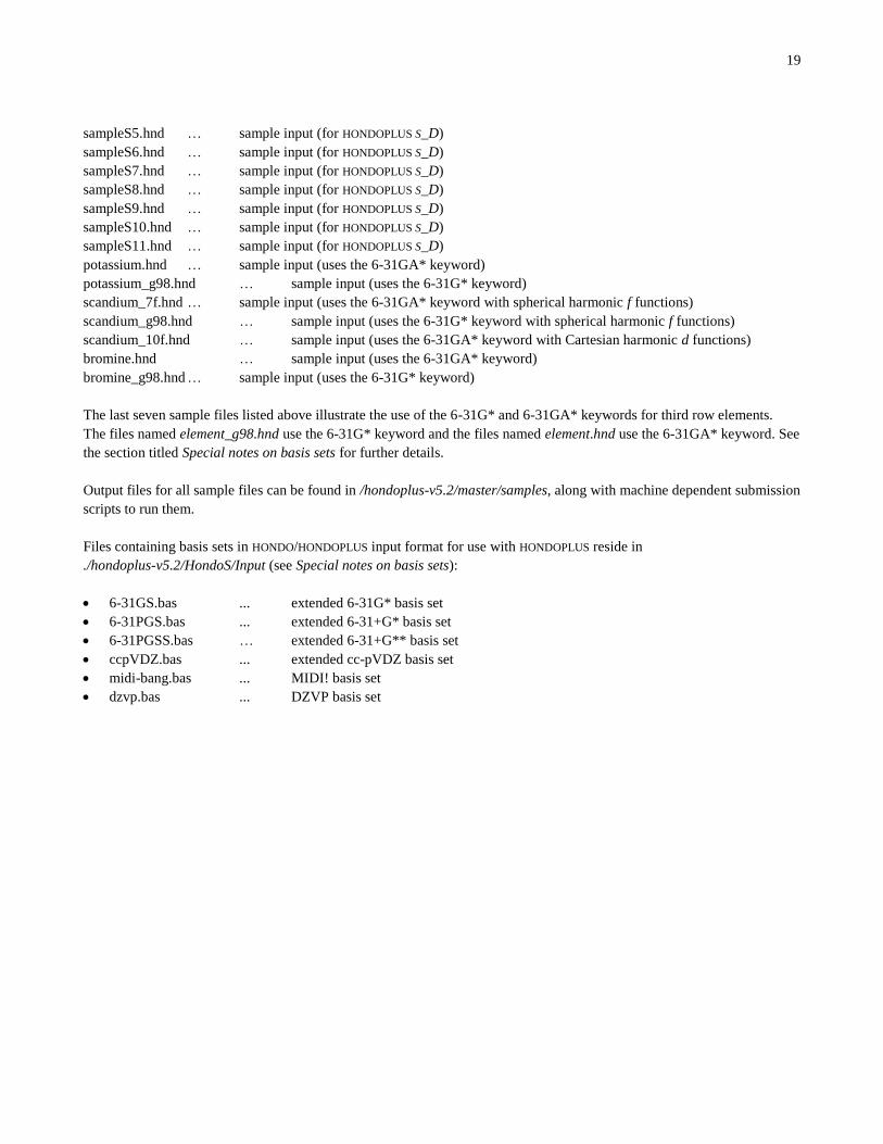
Input sample files reside in hondoplus-v5.2/master/samples:

sample1.hnd ... sample input


























sample26-1.hnd … sample input

sample27.hnd ... sample input ---DISCONTINUED

sample28.hnd … sample input

sampleS1.hnd ... sample input (for HONDOPLUS S)



sampleS4.hnd … sample input (for HONDOPLUS S_D)

19








potassium.hnd … sample input (uses the 6-31GA* keyword)

potassium_g98.hnd … sample input (uses the 6-31G* keyword)

scandium_7f.hnd … sample input (uses the 6-31GA* keyword with spherical harmonic f functions)

scandium_g98.hnd … sample input (uses the 6-31G* keyword with spherical harmonic f functions)

scandium_10f.hnd … sample input (uses the 6-31GA* keyword with Cartesian harmonic d functions)

bromine.hnd … sample input (uses the 6-31GA* keyword)

bromine_g98.hnd … sample input (uses the 6-31G* keyword)

The last seven sample files listed above illustrate the use of the 6-31G* and 6-31GA* keywords for third row elements.

The files named element_g98.hnd use the 6-31G* keyword and the files named element.hnd use the 6-31GA* keyword. See

the section titled Special notes on basis sets for further details.

Output files for all sample files can be found in /hondoplus-v5.2/master/samples, along with machine dependent submission

scripts to run them.

Files containing basis sets in HONDO/HONDOPLUS input format for use with HONDOPLUS reside in

./hondoplus-v5.2/HondoS/Input (see Special notes on basis sets):

6-31GS.bas ... extended 6-31G* basis set

6-31PGS.bas ... extended 6-31+G* basis set

6-31PGSS.bas … extended 6-31+G** basis set

ccpVDZ.bas ... extended cc-pVDZ basis set

midi-bang.bas ... MIDI! basis set

dzvp.bas ... DZVP basis set

20

The test suite input files, output files, and data collection and submission scripts for the charge and solvation models reside

in ./hondoplus-v5.2/HondoS/Input and ./hondoplus-5.1/HondoS/Output. The table below lists the test cases that perfom

each type of calculation:

calculation type test case names

gas-phase Löwdin and CM2 charges test9.02y, y= 1 – 10

SM5.42 single-point energy evaluation in aqueous and

organic solvent

testw.q2y, where w = 1 - 8 and 10, q = 1 and 2, and y = 1,

4, 6, 8, 9, and 10 (only when w = 10)

SM5.42 energy and analytical gradient evaluation in

aqueous and organic solvent


3, 5, 7, and 10 (not when w = 10)

gas-phase Löwdin and CM3 charges by MPWX testw.x.0y, where w = 9 - 12, x = 0, 25, 428, 517, 606, and

999, and y = 315, 316, and 317

testw.x.0y, where w = 1 - 8, x = 999, and y = 315, 316,

and 317

gas-phase RLPA and CM3 charges by MPWX testw.x.0y, where w = 9 - 12, x = 0, 25, 428, 517, 606, and

999, and y = 318 and 319

testw.x.0y, where w = 1 - 8, x = 999, and y = 318 and 319

gas-phase CM3 charges by BLYP and B3LYP test.w.0y, where w = 1 - 12, y = 320 and 321

gas-phase RLPA and CM3 charges by B3LYP/6-31+G* testw.0314, where w = 1 - 12

gas-phase Löwdin and CM3 charges by HF testw.HF.0301, where w = 1 - 12

testw.HF.0302, where w = 1 - 12

testw.HF.0303, where w = 9 - 12

gas-phase Löwdin and CM3.1 charges by HF/MIDI! testw.HF.0322, where w = 1, 4, 5, 6, and 7



testw.x.y, where w = 1 - 8, x = 0, 25, 428, 517, and 606,

and y = 1316, 1317, 2316, and 2317

testw.y, where w = 1 - 8 and y = HF.1303, 1313, HF,

2303, and 2313


organic solvent

testw.x.0y, where w = 1 - 8, x = 0, 25, 428, 517, and 606,

and y = 1315, 1317, 1318, 1319, 2315, 2317, 2318, and

2319


999, and y = 416 and 417


999, and y = 418 and 419

SM6 energy and analytical gradient evaluation in

aqueous solvent

testw.x.y, where w = 1 - 8, x = 0, 25, 428, 517, 606, and

999, and y = 1316 and 1317

SM6 single-point energy evaluation in aqueous solvent testw.x.y, where w = 1 - 8, x = 0, 25, 428, 517, 606, and

999, and y = 1318 and 1319

SM5.42 geometry optimization test13 and test14

generalized Born model calculation test16a-test16b

calculation that utilizes external files test17a-test17b

SM5.42/UHF test case calculation test20

test calculations involving MPWX testx, x = 21-26

generalized Born model + gradient calculation using

RLPA charges

test27

generalized Born model + gradient calculation using

CM3 charges and the new mapping scheme for N and O

test28

SM6 single point energy evaluation of HOOH in

aqueous solvent

test29

SM6 energy and analytical gradient evaluation of

HOOH in aqueous solvent

test30

SM6T single point calculation test31.xy, x=273,298,348, and 373, and y=a and b

SM6T single point calculations at multiple temperatures test32a and test32b


21

using scaled electrostatic contributions

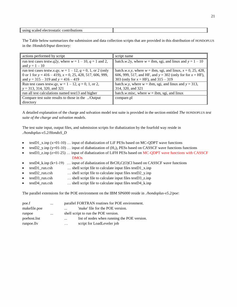
The Table below summarizes the submission and data collection scripts that are provided in this distribution of HONDOPLUS

in the /HondoS/Input directory:

actions performed by script script name

run test cases testw.q2y, where w = 1 – 10, q = 1 and 2,

and y = 1 – 10

batch.w.2y, where w = ibm, sgi, and linux and y = 1 – 10

run test cases testw.x.qy, w = 1 – 12, q = 0, 1, or 2 (only

0 or 1 for y = 416 – 419), x = 0, 25, 428, 517, 606, 999,

and y = 315 – 319 and y = 416 – 419

batch.w.x.y, where w = ibm, sgi, and linux, x = 0, 25, 428,

606, 999, 517, and HF, and y = 302 (only for for x = HF),

303 (only for x = HF), and 315 – 319

Run test cases testw.qy, w = 1 – 12, q = 0, 1, or 2,

y = 313, 314, 320, and 321

batch.w.y, where w = ibm, sgi, and linux and y = 313,

314, 320, and 321

run all test calculations named test13 and higher batch.w.misc, where w = ibm, sgi, and linux

Compare test suite results to those in the ../Output

directory

compare.pl

A detailed explanation of the charge and solvation model test suite is provided in the section entitled The HONDOPLUS test

suite of the charge and solvation models.

The test suite input, output files, and submission scripts for diabatization by the fourfold way reside in

./hondoplus-v5.2/HondoS_D

testD1_x.inp (x=01-10) … input of diabatization of LiF PESs based on MC-QDPT wave functions

testD2_y.inp (y=01-10) … input of diabatization of (H2)2 PESs based on CASSCF wave functions functions

testD3_z.inp (z=01-25) … input of diabatization of LiFH PESs based on MC-QDPT wave functions with CASSCF

DMOs

testD4_k.inp (k=1-19) … input of diabatization of BrCH2C(O)Cl based on CASSCF wave functions

testD1_run.csh … shell script file to calculate input files testD1_x.inp

testD2_run.csh … shell script file to calculate input files testD2_y.inp

testD3_run.csh … shell script file to calculate input files testD3_z.inp

testD4_run.csh … shell script file to calculate input files testD4_k.inp

The parallel extensions for the POE environment on the IBM SP6000 reside in ./hondoplus-v5.2/poe:

poe.f ... parallel FORTRAN routines for POE environment.

makefile.poe ... 'make' file for the POE version.

runpoe ... shell script to run the POE version.

poehost.list ... list of nodes when running the POE version.

runpoe.llv … script for LoadLeveler job

22

Installation

HONDOPLUS version 5.2 has been tested on the following platforms:

Machine Operating System Compiler(s) Makefile

HP Cluster Platform 3000 BL280c Red Hat Linux 4.4.6-4 pgf77 version 12.9 makefile.linux

SGI systems SUSE Linux 3.0.13-

0.27

pgf77 version 11.7-0 makefile.linux

To make the program operational on one of these computer system, go through the following steps:

unzip and untar the distribution file:

gunzip hondoplusv5.2.tar.gz

tar –xvf hondoplusv5.2.tar

Go to the ‘master’ directory:

cd ./hondoplus-v5.2/master

Compile and link the code using one of the makefiles listed in the table above. To install the code with the default

compiler, type

make –f makefile.X

where X is the suffix to one of the makefiles listed in the table above. To install the code using the gnu g77 compiler,

open the appropriate makefile for your system and follow the instructions that appear in the makefile.

23

Run the code:

cd samples

../hondo.x sampleS1.hnd sample1.out &

Further details are given in sections entitled How to compile HONDOPLUS and How to run HONDOPLUS of this manual. From

this point on, we will only be concerned with the description of the capabilities and input options of the program. The next

section contains an overview of the program. Then a detailed description of all the input parameters follows. Comments and

suggestions on how to use the program in some specific situations are also included. Examples of typical calculations

follow. Technical details on how to read the magnetic tape and run the program complete this document.

Overview of HONDO

Capabilities

The following capabilities are available in the present version of the program:

Single configuration self-consistent-field wave functions (closed shell RHF, spin unrestricted UHF, restricted open shell

ROHF),

Generalized valence bond GVB and general multiconfiguration self-consistent-field MCSCF wave functions and

configuration interaction CI wave functions can be calculated.

The electron correlation correction to the energy of closed shell RHF wave functions can be calculated by means of Møller-

Plesset (MP) perturbation theory at second-, third-, and fourth-order (with or without the triples).

The second-order energy correction can be calculated for open shell UHF wave functions.

A generalized Moller-Plesset second-order energy correction for CAS SCF wave functions can be calculated.

Solvation calculations:

SMx (x = 5.42, 5.43, 6 and 6T) solvation model energy for RHF, UHF, and restricted and unrestricted DFT wave

functions using selected basis sets. Analytical gradients and geometry optimizations with the SM5.42, SM5.43,

and SM6 models for restricted and unrestricted HF, DFT, and hybrid DFT wave functions with basis sets using

Cartesian d shells. See Overview of HONDOPLUS for a more complete discussion.

Generalized Born solvation model energies for any restricted or unrestricted HF, DFT, or hybrid DFT wave function,

and analytical gradients and geometry optimizations for any HF, DFT, or byrbid DFT wave function that employs

Cartesian basis functions

Solvent effects can be accounted for via Onsager's Reaction Field model for closed- and open-shell RHF, for open-

shell UHF, and GVB wave functions. Energy gradients can be calculated.

COSMO solvation model energy and gradients for HF, DFT, and MCSCF wave functions.

QM/MM solvation model enengy and gradients for HF, DFT, and MCSCF wave functions using TIP3P-like potentials.

QM/MM solvation model energy and gradients for HF, DFT, and MCSCF wave functions using polarizable MM

potentials.

The effective core potential approximation can be used.

Relativistic one-electron Darwin and mass-velocity terms treated self-consistently.

Optimization of molecular geometries using the gradient of the energy with respect to nuclear coordinates is possible with

all SCF wave functions, and for the MP2 corrected energy for closed-shell SCF wave functions.

Optimization can be carried out in the cartesian space or in the internal coordinate space with the possibility of freezing

some Cartesian or internal coordinates.

24

The force constant matrix in Cartesian space, and the vibrational spectrum, including infrared and Raman intensities, can be

calculated with all cases where analytical gradients of the energy are available (all SCF energies and the closed-shell

MP2 energy).

For closed-shell SCF wave functions, analytical calculation of the force constant matrix is available, for all other cases the

finite difference approach is used.

Calculation of the dipole moment and polarizability derivatives with respect to the nuclear coordinates is possible, for use

with a previously available force constant matrix.

The force constant matrix can be transformed to the internal coordinate basis.

Transition state structures can be determined via calculation of the energy gradients.

The Intrinsic Reaction Coordinate (IRC) pathway can be determined in all case where analytical energy gradients are

available. Note: the IRC is another name for the minimum energy path (MEP) in isoinertial coordinates.

Molecular energies for several points on a potential energy surface can be calculated in a single run.

Non-gradient optimization of basis function exponents is possible. The source code can be modified to carry out

optimization of other non-linear parameters, for example contraction coefficients and even geometrical parameters.

The minimum energy point on the crossing seam surface between two potential energy surfaces can be determined with

RHF, UHF, ROHF, GVB, and MCSCF wave functions.

All wave functions for which the program can compute analytical energy gradients.

The ubiquitous electronic coupling matrix element VAB, for example found in electron transfer formalism can be calculated

with RHF and UHF wave functions. The effects of triple excitations).

The following electronic properties can be extracted from the wave function:

CM2, CM3, and CM4 partial charges for restricted and unrestricted HF, DFT, and hybrid DFT wave functions

Löwdin partial charges for restricted and unrestricted HF, DFT, and hybrid DFT wave functions

redistributed Löwdin populations analsysis charges for restricted and unrestricted HF, DFT, and hybrid DFT wave

functions

Mulliken population analysis

valency and bond order analysis

dipole moment

quadrupole moment

octapole moment

spin density at the nuclei

electrostatic field at the nuclei

electrostatic field gradient at the nuclei

hyperfine interactions (Fermi contact term and anisotropic interaction)

orbital localization

electron and spin density maps

electrostatic potential maps

sum-over-states (hyper)polarizabilities

dipole polarizabilities and hyperpolarizabilities

frequency dependent (hyper)polarizabilities

Stone's distributed multipole analysis and electrostatic potential

Potential-derived-charges

Chemical shift tensors using GIAO formalism for SCF closed shell wave functions

The potential due to finite point charges for a classical representation of an environment, or a uniform electric field can be

incorporated into the one-electron Hamiltonian.

Conversion data are created to use as input data for other programs:

the structure plotting program from GAMESS

the orbital/density plotting program from GAMESS

Bader's AIMPAC program

Bouman's RPAC program

25

`

Other features are as follows:

The program uses Gaussian-type basis functions with angular momentum s, p, d, f, and g (g functions may not be used

when using effective core potentials if the energy gradient is requested or when analytical calculation of the second

derivative matrix is requested; f functions can be used for Löwdin and RLPA, calculations. This version of the code can

handle up to 128 atoms and 512 shells for a total of 2048 unique gaussian exponential functions; RHF, UHF, ROHF, GVB,

CAS, MC, and MP2 calculations are no longer limited to a maximum of 255 basis functions. For all the other types of

energy calculation, the 255 basis function limit is still enforced. There is a maximum of 3072 basis functions allowed in all

cases, even for direct algorithms.

Vectorization

Some substantial effort has been put into the vectorization of various modules of the code wherever appropriate.

Vectorization appears under two different forms: use of the library of vectorized routines, and explicit vectorization.

Key subroutines that contain calls to routines available in the IBM Engineering And Scientific Subroutines Library (ESSL)

have been grouped together in hondo_ibm.f and hondo_linux.f. For SGI platforms, calls to the same subroutines that are

available in the linear algebra package (LAPACK) have been grouped together in the hondo_sgi.f. It is intended that the

subroutines in these files will replace the subroutines with the same name that can be found in the other 'master' files. In

order to activate the vectorized code the user need only to link the file hondo_ibm.f or hondo_sgi.f ahead of the other files.

Many subroutines have been modified for better detection of vector operations by the compiler. These routines ought to be

compiled with the vectorizing option turned on.

Finally in the subroutine HONDO of the file ctl.f the logical variable VECTOR is defined to indicate whether the code can

make use of the vectorizing Fortran compiler or not. This applies presently only to the electron repulsion integral module

int.f and their derivatives der.f, and hss.f. If VECTOR=.TRUE., the routines modified for vectorization will be executed. If

VECTOR=.FALSE., then only the scalar forms of the routines will be executed.

Parallelization

Software is provided to run the program in a parallel mode, for distributed-memory systems. In particular the software

additions to run under the POE, MPI, PVM3 and TCGMSG environments are included on the tape. The installation

directives mentioned in the appropriate sections of this manual assume that POE, MPI, PVM3 and/or TCGMSG have been

installed and are operational. Note that only selected functions have been implemented in parallel. RHF, UHF, ROHF, and

GVB energy and gradient calculations, as well as MP2 energy calculations are set up to run in parallel execution mode.

The current SGI version of HONDO does not run in parallel.

Memory management

The memory is dynamically allocated, depending on the number of basis functions. A common block labelled /SCM/

defines the working area where the data manipulation is done in most of the modules of the program. When a calculation

requires more memory than defined in /SCM/ the program stops. If needed, the user can increase or decrease the size of the

COMMON block /SCM/ by changing the dimension of the block and specifying the appropriate memory size in the

variable MEMSCM which is defined in a DATA statement. These two changes must be done in the ‘main’ program

26

HND99 in the file hondo_ibm.f, hondo_sgi.f or hondo_linux.f (for the POE version the changes have to be made in the file

poe.f, for the MPI version in the file mpi.f, for the PVM3 version in the file pvm.f, for the TCGMSG version in the file

tcg.f).

The common block /SCM/ is used as working area for most of the modules. No data is permanently stored there, i.e. any

data stored there is subject to be written over by some other module, so that all necessary data for the execution of a

particular module must be read into memory at the start of the execution of the module.

The common block /LCM/ is used in a different way. If /LCM/ is big enough to hold the two electron repulsion integrals

over atomic functions, then those integrals are stored there and the calculation proceeds in the 'in-memory' mode, rather

than in the traditional way in which an integral file is created on disk. /LCM/ may be too small to hold the integrals, but it

may be large enough that supermatrices can be generated in canonical order on the fly via a temporary storage into /LCM/ .

The SCF, UHF, ROHF, GVB, MP2, and MCSCF modules can all work with integrals 'in-memory' or sorted supermatrices,

which reduces the computer time. The code decides which algorithm to use on the basis of the size of these two common

blocks.

Memory size requirements

No overlay directives are provided to link and load the program as the virtual memory management of the operating system

manages the pages of the code. The source code requires approximately 16 megabytes (MB) of memory to load, exclusive

of the memory required for the common blocks /SCM/ and /LCM/ . The size of these common blocks then determines the

total region size for the program. If /SCM/ is 500000 words long and /LCM/ 250000 words long, then they occupy 4

megabytes and 2 megabytes, and the total region size needed to load HONDO is about 22 MB .

In addition, the common block /LCM/ is also used to hold the electron repulsion integrals when the in-memory algorithms

are in operation. This applies to RHF and UHF SCF and MP2 energy calculations only right now. The size of the /LCM/

common block may be changed in a way similar to the /SCM/ common block.

AIX, IRIX, and Linux implementations

To make HONDOPLUS compatible with the IBMs, SGIs, and machines running Linux, all system dependent routines have

been grouped together into files hondo_ibm.f, hondo_sgi.f, and hondo_linux.f. In the process of making HONDOPLUS

compatible on the SGI architecture, we discovered several problems with the way the program reads namelists. If two

namelists names begin with the same series of characters, with one of the namelist names being longer than the other

namelist name, the program does not always distinquish between the two in the input file. This appears to be a bug in the

F90 compiler for IRIX systems. The following is a summary of a solution to this problem:

The $MM namelist name is now referred to as $MMNOPOL. This namelist is used to define parameters for a non-

polarizable molecular mechanics solvent. The name of this namelist has been changed to avoid conflicts with the

$MMPOL namelist, which is used to define a polarizable molecular mechanics solvent. A sample calculation

(sample26-1.hnd) has been added to the HONDO test suite to illustrate the use of this new namelist name.

The $OPTZ namelist is now referred to as $FREZ. This namelist is generated internally by the program, and is used to

define frozen internal coordinates in a geometry optimization. This name change was made to avoid conflicts with the

$OPT namelist. Note that the user may define the $FREZ namelist in his or her input file, but we found that the

program ignores it in both the SGI and IBM versions of the code. (This was also the case for the $OPTZ namelist). To

specify internal coordinates as frozen, we suggest using the features of the $GEO data group (see the section entitled

27

Data group $GEO). A sample calculation (sample28.hnd) has been added to illustrate the use of this new namelist

name.

If the $QM namelist and the $QMMM data group are defined in the same input, the $QM namelist must always occur first.

Although the information supplied by the $QMMM data group is not formally aquired in the same way it would be if it

were a namelist, the program still may try to interpret it as the $QM namelist. A sample calculation (sample26-1.hnd)

has been added to illustrate the way these two namelist should be used.

If the $GUGDM and $GUGDM2 namelists are defined in the same input, the $GUGDM namelist must always occur first.

Note that other namelists and data groups with similar names exist, but we have tested their use extensively and found no

problems with them.

Finally, the user needs to be careful of the types of characters used in the title section of the $GEO data group. On the SGI

version of HONDOPLUS, the program may misinterpret the ‘/’ character and other special characters. It appears that the

program will ignore all namelists and use default settings. To avioid this problem, place single or double quotation marks

around the title in the $GEO data group when the title contains special characters, see sample28.hnd and test22.in in the

test suite.

An additional problem seen with some compilers occurs when a logical variable is included in the input. If the value of the

logical variable is not enclosed in periods the program will ignore the following variable, ie ReadK=TRUE may cause

problems whereas ReadK=.True. or ReadK=.T. should not.

Restart capabilities

The program checks for CPU time, and it can be stopped and restarted where it left off. The restart data is printed and

punched automatically on file FT07. A restart value of IREST = 1 works always and is very safe. Other restart options may

not work in all cases because of the complexity of the program. More information is available with the description of the

IREST parameter in the namelist $CNTRL.

The direct access file DA10 must have been allocated permanently on disk at the end of the initial run, and must be

accessed for the continuation run, as it contains information pertinent to the calculation.

The direct access file DA10

The file DA10 is a direct access file used throughout the program to store important data, such as the molecular orbital

coefficients, and other pieces of information. This file is needed for a restart job, as the first record on the file contains

many parameters values saved when the initial job terminated. The directory of the DA10 file is listed in a section of the

documentation below.

Input

Free format (see AIX, IRIX, and Linux Implementations for several notable exceptions) NAMELIST is used to input the

data. In some cases the input is read as a data group which is a collection of data with a fixed format and is preceded with a

keyword characteristic of the data. Note that we are currently switching to home-made 'free-format' input for some of these

data groups for ease-of-use, specifically $BASIS, $ECP, $EFC, $XYZ, and $DRT. The home-made free-format differs

from the standard free-format in that character strings need not be surrounded by quotes, so that fixed-format data of old

may be read as is in most cases. In doing so we are able to maintain a high level of compatibility with the old fixed-format

input. However note that free-format input requires that all input parameters be given specifically, so that in some cases the

old input data will not work. Also, any two input parameters have to be separated by a blank space, so that some old input

28

data may not be interpreted correctly. This is mostly true for the $ECP data group. Finally character strings may not contain

blanks within them, something that was allowed in the fixed-format input of old. A description of the namelists and data

groups follows in the next sections.

The traditional way of inputting the data to the program is to create a suitable input file with a text editor. However a much

more convenient way of preparing an input file is to make use of the interactive window-based interface of KGNGRAF.

This interface is menu-driven and allows the user to select most different options through pop-up windows. Use of

KGNGRAF eliminates the need to know the format of the input file, to be aware of all possible options for all the input

parameters, and their hierarchical relations. KGNGRAF is a "friendly" graphical interface that provides numerous other

capabilities tailored to electronic structure studies. KGNGRAF was developed by Steven Chin from IBM-Kingston.

Note that at the very start of the program the input file (FT05) is copied onto FT04, which is then used by the program as

the input file. The program rewinds FT04 each time it searches for a particular namelist or data group. So there are no

restrictions on the order in which the input data is given (see AIX, IRIX, and Linux Implementations for several notable

exceptions), comment cards may be inserted into the input file and will be ignored by the program, and multiple

occurrences of namelists or data group are allowed. In this case the program uses the first occurrence of a namelist or of a

data group. This is of course quite convenient, as a file can contained several versions of a data group , but there are also

drawbacks, as it is easy to make mistakes and use the wrong data.

A recent enhancement to the program is its Z-matrix compatibility. Z-matrix is the term used to characterize the method of

input of the atoms of the molecule, whereby the atomic connectivity is specified along with bond lengths, bond angles,

torsion angles, and the like. Additionally several basic functions can be invoked by use of key words. To this end the

program makes use of four newly defined free-formatted data groups. These data groups are $JOB , $BAS , $GEO, and

$SYM. Because they provide a very simple way to define a calculation, these data groups will be presented first.

Before going on to the specification of the namelists and data group, we want to emphasize that only one data group is

absolutely required to run the program. It is one of the two data groups $BASIS or $GEO .The other data groups and

namelists may be omitted if the user is satisfied with the default values of other parameters.

Overview of HONDOPLUS

HONDOPLUS contains two additional modules that have been added to the HONDO 99 code. The first is a module for

incorporation of Löwdin charges and redistributed Löwdin population analysis (RLPA) charges, the CM2, CM3, and CM4

charge models, and the SM5.42, SM5.43, SM6, and generalized Born (GB) solvation models. The second is a module to

calculate diabatic states based on configurational uniformity and the fourfold way.

In order to make the following clear, we note that the following basis sets involve Cartesian d functions:

MIDI!6D (also known as MIDIX6D)

6-31G*

6-31+G*

6-31+G**

DZVP

and the following basis sets involve spherical harmonic d functions:

MIDI! (also known as MIDI!5d, MIDIX, and MIDIX5D)

cc-pVDZ

29

Executive summary for the charge and solvation models

Gas-phase and liquid-phase Löwdin partial atomic charges can be obtained for all restricted and unrestricted Hartree-

Fock (HF), density-functional theory (DFT), and hybrid DFT wave functions. For calculations using the 6-31+G*

and 6-31+G** basis sets, gas-phase and liquid-phase redistributed Löwdin population analysis (RLPA) partial

atomic charges can be obtained for all restricted and unrestricted HF, DFT, and hybrid DFT methods.

Gas-phase and liquid-phase Löwdin partial atomic charges can be obtained for all restricted and unrestricted Hartree-

Fock (HF), density-functional theory (DFT), and hybrid-DFT wave functions. For calculations using the 6-31+G*

and 6-31+G** basis sets, gas-phase and liquid-phase redistributed Löwdin population analysis (RLPA) partial

atomic charges can be obtained for all restricted and unrestricted HF, DFT, and hybrid DFT methods.

Gas-phase and liquid-phase CM2 class IV charges can be determined for the following combinations of electronic

structure theory and basis set (using either a restricted or an unrestricted formalism):

HF/MIDI! B3LYP/MIDI!

HF/MIDI!6D BPW91/6-31G*

HF/6-31G* HF/6-31+G*

BPW91/MIDI! HF/cc-pVDZ

BPW91/MIDI!6D BPW91/DZVP



HF/MIDI!6D HF/6-31G*

MPWX/MIDI! MPWX/MIDI!6D

MPWX/6-31G* MPWX/6-31+G*

MPWX/6-31+G** BLYP/6-31G*

B3LYP/MIDI!6D B3LYP/6-31G*

B3LYP/6-31+G*

MPWX is a method that uses the mPW exchange functional of Adamo and Barone (Adamo, C.; Barone, V. J. Chem. Phys.

1998, 108, 664), the PW91 correlation functional (Perdew, J. P. Electronic Structure of Solids '91; Zieesche, P., Eshrig, H.,

Eds.; Akademie: Berlin, 1991) and a percentage of HF exchange, X. Note that MPWX includes the following special cases:

MPW0 mPWPW91

MPW6 MPW1S

MPW25 mPW1PW91

MPW42.8 MPW1K

MPW60.6 MPW1KK

For all of the MPWX methods listed above, CM3 has been parameterized for five specific values of X, namely 0, 25, 42.8,

60.6, and 99.9, and these parameter sets are available in HONDOPLUS. Every CM3 and CM4 parameter is a linear or a

30

quadratic function of the percentage of HF exchange used in the mPW exchange functional. So, in addition to the specific

CM3 and CM4 parameter sets (i.e. when X in MPWX is 0, 25, 42.8, 60.6, and 99) the CM3 and CM4 Charge Models are

available for any value of X in MPWX between 0.0 and 99.9. The details of this correction are described fully in “The

Effectiveness of Diffuse Basis Functions for Calculating Relative Energies”by Density Functional Theory” by Lynch, B. J.;

Zhao, Y.; Truhlar, D. G. J. Phys. Chem. A, 2003, 107, 1384.

The CM3 model for the BLYP and B3LYP methods uses a slightly modified mapping scheme for compounds that contain

N and O. For more information, see “Parameterization of Charge Model 3 For AM1, PM3, BLYP, and B3LYP” by

Thompson, J. D.; Cramer, C. J.; Truhlar, D. G. J. Comput. Chem., 2003, 24, 1291. We have also developed a special CM3

model for assigning partial atomic charges to high-energy materials. This model is called CM3.1, and it uses the same

mapping scheme as the CM3 model for BLYP and B3LYP. This model has been parameterized for use with HF/MIDI!,

and is described in “Accurate Partial Atomic Charges for High-Energy Molecules with the MIDI! Basis Set” by Kelly, C.

P.; Cramer, C. J.; Truhlar, D. G. Theor. Chem. Acc., 2005, 113, 133.



BLYP/MIDI!6D BLYP/6-31+G*

BLYP/6-31G* BLYP/6-31+G**

BPW91/MIDI!6D BPW91/6-31+G*

BPW91/6-31G* BPW91/6-31+G**

B3LYP/MIDI!6D B3LYP/6-31+G*

B3LYP/6-31G* B3LYP/6-31+G**

B3PW91/MIDI!6D B3PW91/6-31+G*

B3PW91/6-31G* B3PW91/6-31+G**

MPWX/MIDI!6D MPWX/6-31+G*

MPWX/6-31G* MPWX/6-31+G**

Liquid-phase calculations based on gas-phase geometries can be performed with SM5.42 for the following restricted

and unrestricted Hartree-Fock, DFT, and adiabatic-connection-method wave functions (i.e. hybrid DFT wave

functions) that employ spherical harmonic or Cartesian d functions:

HF/MIDI! B3LYP/MIDI!

HF/MIDI!6D BPW91/6-31G*

HF/6-31G* HF/6-31+G*

BPW91/MIDI! HF/cc-pVDZ

BPW91/MIDI!6D BPW91/DZVP

31

Liquid-phase calculations based on gas-phase geometries can be performed with SM5.43 for the following restricted

and unrestricted Hartree-Fock, DFT, and adiabatic-connection-method wave functions (i.e. hybrid DFT wave

functions) that employ spherical harmonic or Cartesian d functions:

HF/6-31G* B3LYP/6-31G*

MPWX/MIDI! MPWX/MIDI!6D

MPWX/6-31G* MPWX/6-31+G*

MPWX/6-31+G**

Liquid-phase calculations based on gas-phase geometries can be performed with SM6 for the following restricted and

unrestricted DFT and adiabatic-connection-method wave functions (the four basis sets for which SM6 is

parameterized use Cartesian d functions):

BLYP/MIDI!6D BLYP/6-31+G*

BLYP/6-31G* BLYP/6-31+G**

BPW91/MIDI!6D BPW91/6-31+G*

BPW91/6-31G* BPW91/6-31+G**

B3LYP/MIDI!6D B3LYP/6-31+G*

B3LYP/6-31G* B3LYP/6-31+G**

B3PW91/MIDI!6D B3PW91/6-31+G*

B3PW91/6-31G* B3PW91/6-31+G**

MPWX/MIDI!6D MPWX/6-31+G*

MPWX/6-31G* MPWX/6-31+G**

Liquid-phase analytical gradients are available for basis sets that use Cartesian d shells, namely:

MIDI!6D 6-31G*

6-31+G* 6-31+G**

DZVP

The availability of liquid-phase analytical gradients allows for efficient geometry optimization of liquid-phase minima

and saddlepoints and for liquid-phase evaluation of numerical Hessians and vibrational frequencies based on

liquid-phase analytical gradients.

Generalized Born electrostatic solvation energy calculations using Löwdin partial atomic charges are available for all

restricted and unrestricted HF, DFT, and hybrid DFT wave functions that use any Cartesian or spherical harmonic

basis set as long as the basis set does not contain functions of higher angular momentum than f. For methods using

the 6-31+G* and 6-31+G** basis sets, generalized Born electrostatic solvation energy calculations using

redistributed Löwdin population analysis (RLPA) partial atomic charges are also available for all restricted and

unrestricted HF, DFT, and hybrid DFT methods.

32

Analytical gradients of the generalized Born electrostatic solvation energy using Löwdin or RLPA partial atomic

charges are available for all RHF, UHF, DFT, unrestricted DFT, and restricted and unrestricted hybrid DFT wave

functions that use Cartesian d and f basis functions. Where analytical gradients are available, so are geometry

optimizations of liquid-phase minima and saddle points, and the evaluation of liquid-phase numerical Hessians and

vibrational frequencies based on liquid-phase analytical gradients.

Löwdin population analysis and redistributed Löwdin population analysis

Löwdin population analysis, like Mulliken population analysis, provides class II atomic partial charges, but the Löwdin

method has certain advantages. It was added to the code because it is the first step in the CM2 and some of the CM3 and

CM4 charge models (redistributed Löwdin population analysis is used for the other CM3 and CM4 models). Having added

this capability, there may be some independent interest in Löwdin population analysis since it can be used with any basis

set, whereas CM2 and CM3 can only be used for combinations of level and basis set for which parameters are available.

(For CM4, calculations that employ any good density functional, along with the MIDI!6D, 6-31G*, 6-31+G*, and

6-31+G** basis sets, can be performed.) It is expected that Löwdin’s method will often yield more useful population

analyses than Mulliken’s method.

Partial atomic charges obtained from Löwdin population analysis can, however, be sensitive to basis set size, particularly

for extended basis sets that include diffuse functions. We have developed and implemented a new method, called

redistributed Löwdin population analysis (or RLPA), which alleviates some of this sensitivity to basis set size. RLPA

charges are used as the starting point for CM3 charges when the 6-31+G* or 6-31+G** basis set is used.

Charge Model 2, Charge Model 3, and Charge Model 4

Charge Model 2 (CM2), Charge Model 3 (CM3), and Charge Model 4 (CM4) are our second-, third-, and fourth-generation

models of class IV charges, respectively. Charge Model 3 has been parameterized with a larger training set than CM2 (398

data vs. 198 data), and it is available for different combinations of electronic structure theory and basis sets than CM2.

Furthermore, it is parameterized for Li and for molecules that contain Si-O, Si-F, and Si-Cl bonds (CM2 is not). Charge

Model 4 has been parametrized against the same training set that CM3 was, except that CM4 gives improved charges for

aliphatic functional groups, which is important for modeling hydrophobic effects. Class IV charges are obtained by a

semiempirical mapping of class II charges defined for a particular basis set. CM2, CM3, and CM4 use the same

semiempirical mapping scheme. Class IV charges have the following advantages over class III charge models available in

Gaussian (e.g., ChElPG and Merz-Kollman algorithms):

Class III charges are unreliable for buried charges (this problem is widely recognized, as discussed in work by Kollman and

Francl and their respective coworkers). Class IV charge models provide a practical and stable way to obtain reasonable

charges for buried atoms.

Class III charges are at best as good as the basis set and wave function used, whereas class IV charges represent

extrapolation to full CI with a complete basis.

Class IV charges are useful for any purpose for which ChElPG or Merz-Kollman charges are useful, but we believe that

they are better.

33

SMx (x = 5.42, 5.43, 6, and 6T) Solvation Models

SM5.42, our earliest solvation model implemented in HONDOPLUS, is a universal Solvation Model based on SM5 functional

forms for atomic surface tensions (hence the first three characters in the name of the method are SM5), built on class IV

point charges (hence .4 comes next) of the CM2 type (hence 2). A more recent model, called SM5.43, uses the same

functional forms for atomic surface tensions as does SM5.42, but SM5.43 uses CM3 charges (hence the 3 in the name).

Our most recent solvent model, called SM6, is based on SM6 functional forms for atomic surface tensions and uses class IV

CM4 point charges. The SM6T solvation model is an extension of SM6 to include the temperature dependence of the free

energy of solvation relative to 298 K. It uses SM6 to compute the free energy of solvation at 298 and uses additional atomic

surface tensions with the same functional form as SM6 to compute the temperature dependence of the free energy of

solvation.

The SMx solvation models provide a way to calculate electronic wave functions in liquid-phase solution and free energies

of solvation. The SM5 models are universal, i.e., parameterized for water and any organic solvent. With universal models,

if desired, one can calculate solvation free energies for two different solvents (e.g., water and 1-octanol) and use the results

to calculate log P, where P is the partition coefficient. Presently, the SM6 and SM6T models have only been parametrized

for aqueous solvent.

For solvation calculations based on gas-phase geometries, the standard-state free energy of solvation )(o

S RG is given by

two components:

CDSEP

o

S )( GGG R (1)

where

PEEP GEG (2)

In equations (1) and (2), GEP is the bulk electrostatic component of the solvation free energy; it is the sum of the

polarization energy GP (representing favorable solute-solvent interactions and the associated solvent rearrangement cost)

and the distortion energy EE (the cost of distorting the solute electronic charge distribution to be self-consistent with the

solvent electric polarization). GCDS accounts for first-solvation-shell effects.

GEP is determined by a self-consistent reaction field (SCRF) calculation, which allows the solvent-induced change in the

solute electronic wave function to be optimized variationally. GCDS is not a self-consistent term; it has no effect on the

solute electronic wave function. In its simplest form GCDS is defined as:

k

kkAG CDS (3)

where Ak is the exposed surface area of atom k (this depends on the solute’s 3-D geometry and is calculated by the

Analytical Surface Area (ASA) algorithm as described in reference LH95 and as included in recent versions of AMSOL,

and k is the atomic surface tension of atom k. The atomic surface tension k is itself a function of the solute’s 3-D

geometry and a small set of solvent descriptors. References LH98, ZL98, and LZ99 present a more expanded form of

GCDS than what appears in equation (3):

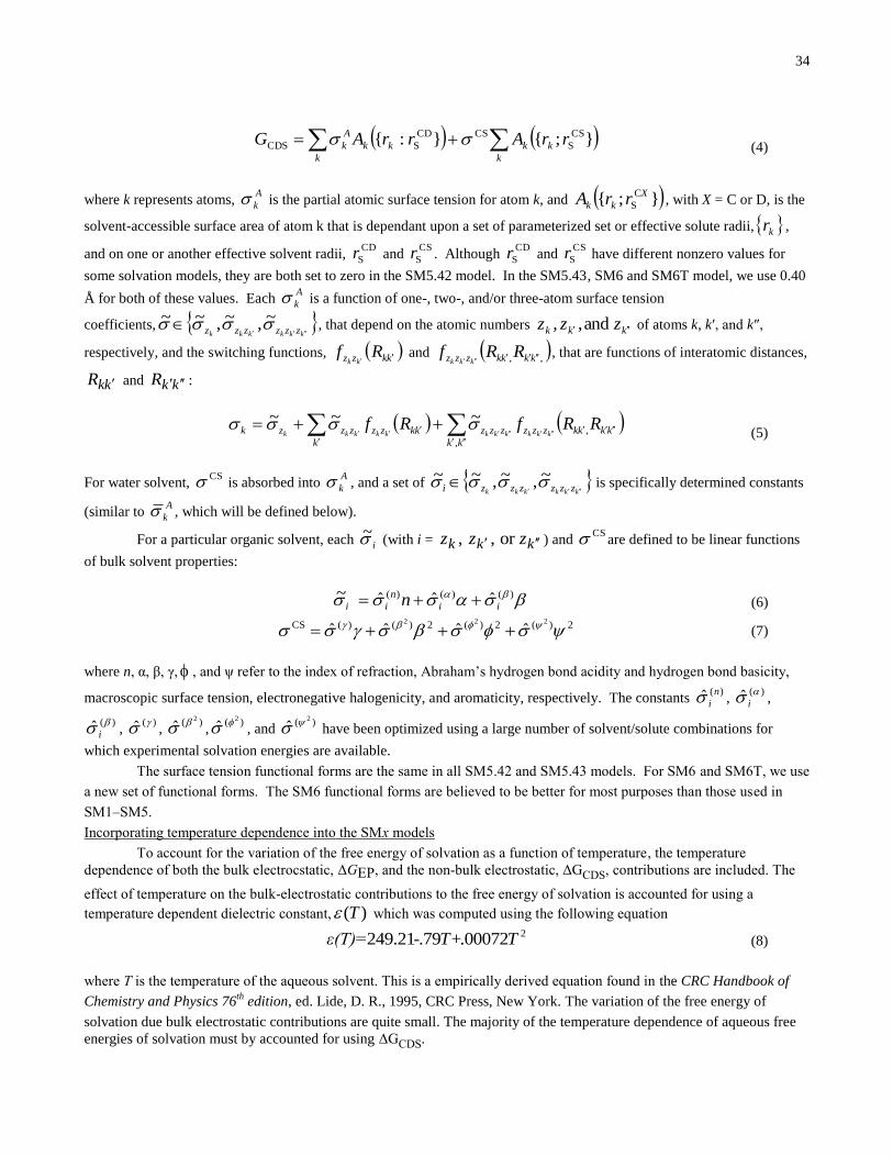
34

};{}:{ CS

S

CSCD

SCDS rrArrAG k

k

kkk

k

A

k (4)

where k represents atoms, A

k is the partial atomic surface tension for atom k, and };{ C

S

X

kk rrA , with X = C or D, is the

solvent-accessible surface area of atom k that is dependant upon a set of parameterized set or effective solute radii, kr ,

and on one or another effective solvent radii, CD

Sr and CS

Sr . Although CD

Sr and CS

Sr have different nonzero values for

some solvation models, they are both set to zero in the SM5.42 model. In the SM5.43, SM6 and SM6T model, we use 0.40

Å for both of these values. Each A

k is a function of one-, two-, and/or three-atom surface tension

coefficients, kkkkkk zzzzzz

~,~,~~, that depend on the atomic numbers kkk zzz and,, of atoms k, k′, and k″,

respectively, and the switching functions, kkzz Rfkk

and ,, kkkkzzz RRfkkk

, that are functions of interatomic distances,

kkR and kkR :

kk

kkkkzzzzzz

k

kkzzzzzk RRfRfkkkkkkkkkkk

,

,~~~

(5)

For water solvent, CS is absorbed into

A

k , and a set of kkkkkk zzzzzzi

~,~,~~ is specifically determined constants

(similar to A

k , which will be defined below).

For a particular organic solvent, each i~ (with i = kkk zzz or ,, ) and CS are defined to be linear functions

of bulk solvent properties:

)()()( ˆˆˆ~ ii

n

ii n (6)

2)(2)(2)()(CS 222

ˆˆˆˆ (7)

where n, α, β, γ, , and ψ refer to the index of refraction, Abraham’s hydrogen bond acidity and hydrogen bond basicity,

macroscopic surface tension, electronegative halogenicity, and aromaticity, respectively. The constants )(ˆ n

i , )(ˆ i ,

)(ˆ i , )(ˆ ,

)( 2

ˆ ,)( 2

ˆ , and )( 2

ˆ have been optimized using a large number of solvent/solute combinations for

which experimental solvation energies are available.

The surface tension functional forms are the same in all SM5.42 and SM5.43 models. For SM6 and SM6T, we use

a new set of functional forms. The SM6 functional forms are believed to be better for most purposes than those used in

SM1–SM5.

Incorporating temperature dependence into the SMx models

To account for the variation of the free energy of solvation as a function of temperature, the temperature

dependence of both the bulk electrocstatic, ΔGEP, and the non-bulk electrostatic, ΔGCDS, contributions are included. The

effect of temperature on the bulk-electrostatic contributions to the free energy of solvation is accounted for using a

temperature dependent dielectric constant, )(T which was computed using the following equation

200072.79.21.249 TT+-ε(T)= (8)

where T is the temperature of the aqueous solvent. This is a empirically derived equation found in the CRC Handbook of

Chemistry and Physics 76th

edition, ed. Lide, D. R., 1995, CRC Press, New York. The variation of the free energy of

solvation due bulk electrostatic contributions are quite small. The majority of the temperature dependence of aqueous free

energies of solvation must by accounted for using ΔGCDS.

35

In SM6T the ΔGCDS term mimics the thermodynamic equation for the temperature dependence of free energies of

solvation where the thermodynamic properties, the heat capacity and the entropy of solvation, have been replaced

parameterized atomic surface tensions:

k

C

kk

k

B

kk AT

TTATTG 298

ln298298)(CDS (9)

where B

k and C

k are atomic surface tensions with identical functional forms to those of k. Caution should be used in

assigning any physical meaning to the atomic surface tensions shown above. Note that the model has only been developed

for C, H, and O containing compounds in aqueous solutions for the temperature 273 to 373 K.

A comment on using gas-phase geometries to calculate solvation free energies.

For SM1–4 and SM5.4, geometry optimization in solution was an essential part of the parameterization. SM5.42,

SM5.43, SM6 and SM6T are parameterized in such a way that one fixes the geometry at a reasonable value (any reasonably

accurate gas-phase geometry should be acceptable) and calculates the solvation energy without changing the geometry.

Thus, geometry optimization in the presence of solvent is not required to obtain accurate solvation free energies. This

method of obtaining solvation parameters based on gas-phase geometries was adopted for several reasons. First, previous

experience has shown that the difference one gets from re-optimizing the geometry in the presence of solvent in almost all

cases is small—less than the average uncertainty in the method or in any competing method. Second, for many solutes,

less expensive (e.g. semiempirical or molecular mechanics methods) can yield accurate gas-phase geometries. Third, for

other solutes, such as transition states, solutes with low-barrier torsions, multiple low-energy conformations, weakly bound

complexes, and in cases where one or more solvent molecules are treated explicitly, more expensive levels of theory might

be needed to yield accurate geometries. Finally, solvation energies obtained using gas-phase geometries can be added

conveniently to gas-phase energies for separable-equilibrium-solvation dynamics calculations.

In some cases, geometry optimization in the presence of solvent is important. In these cases, one can also apply

the SM5.42, SM5.43, or SM6 models at a solute geometry R that is not an approximation to an equilibrium gas-phase

geometry. This type of calculation corresponds to the fixed-R solvation energy, which is still given by )(o

S RG of

equation (1). Evaluation of this quantity for geometries that do not correspond to an equilibrium structure is useful for

dynamics calculations because the potential of mean force is given by

)()()( o

S RRR GVW (10)

where VI is the gas-phase potential energy surface (which is itself given by the sum of the gas-phase electronic energy and

the gas-phase nuclear repulsion energy). If one applies the SM5.42, SM5.43, or SM6 models to a geometry optimized in

solution and subtracts the gas-phase energy at a geometry optimized for the gas phase, one obtains the true solvation energy

for the given method.

Note that both free energies of solvation and potentials of mean force depend on temperature; all of our solvation

models except SM6T are currently only parameterized for a single temperature, namely 298 K.

Furthermore )(o

S RG depends on standard state choices; the values given directly by the SM5 models

correspond to using the same molar density (e.g., one mole per liter) in the gas phase and in the liquid-phase solution.

Furthermore the liquid-solution standard state corresponds to an ideal dilute solution at that concentration. However, one

may adjust the results to correspond to other choices of standard state by standard thermodynamic formulae. Note that

36

changing the standard state corresponds to adding a constant to WI; thus the gradient of WI, which is used for dynamics, is

not affected.

Analytical gradients and geometry optimizations

Analytical gradients of SM5.42, SM5.43, and GB liquid-phase wave functions have been implemented in HONDOPLUS

beginning with version 3.0. In particular, HONDOPLUS contains analytical gradients for restricted and unrestricted wave

functions and for basis sets that employ Cartesian basis functions. However, analytical gradients are still not available SCF

scheme III, and for basis sets with spherical harmonic d and f functions.

The availability of gradients allows for efficient geometry optimization in liquid-phase solution. This is necessary in many

cases. For example, the transition state geometry for the SN2 reaction of ammonia and chloromethane (the Menschutkin

reaction) depends strongly on solvent. Other applications include the study of phase-dependent reaction mechanisms and

molecular conformational preferences.

Equation (1) can be rewritten as:

GSo(R) Go(l,Re(g))G

o(g,Re(g)) (11)

where )(o

S RG is the difference in the standard-state free energy of a molecular species fixed in its gas-phase equilibrium

geometry, )(gRe , in liquid-phase solution, l, and in the gas phase, g. Furthermore,

))(())(())(,())(,( CDSP

o gRGgRGgRlEgRlG eeee (12)

and

))(,())(,(o gRgEgRgG ee (13)

where ))(,( gRlE e is the SCRF energy in the presence of the solvent, while ))(,( gRgE e is the gas-phase SCF energy.

Geometry optimization in solution yields the solute equilibrium geometry, )(lRe . In the SM5.42, SM5.43, and

SM6 models, the definition of o

SG is analogous to the definition of )(o

S RG in equation (9):

))(,())(())(())(,(

))(,())(,(

CDSP

ooo

S

gRgElRGlRGlRlE

gRgGlRlGG

eeee

ee

(14)

A full derivation of the analytical gradient is presented in the paper by T. Zhu et al. entitled “Analytical Gradients

of a Self-Consistent Reaction-Field Solvation Model Based on CM2 Atomic Charges” (J. Chem. Phys. 1999, 110, 5503-

5513).

Note that the current implementation of SM6T cannot be used to optimize solute geometries.

SCRF calculations using the generalized Born model and CM2, CM3, or CM4 charges

A self-consistent-reaction-field method based on the generalized Born approximation and CM2, CM3, or CM4

charges has been implemented in the program. One can use the SCRF orbitals to calculate the polarization and distortion

energies and solvated atomic partial charges and to investigate solvation effects on the atomic charge distribution, multipole

moments, and other one-electron properties. In addition, the SCRF calculation is one of the two components of a

calculation of the free energy of solvation.

37

Allowed Combinations of Solvent Model, Electronic Structure Theory, and Basis Set.

When using HONDOPLUS, the SM5.42 models should only be applied with the ten combinations of basis sets and

density functionals for which parameters are currently available in Gaussian:

Standard notation keyword(s) notes

HF/MIDI! HF/MIDIX

HF/MIDI!6D HF/MIDIX 6D

HF/6-31G* HF/6-31G*

BPW91/MIDI! BPW91/MIDIX

BPW91/MIDI!6D BPW91/MIDIX 6D

B3LYP/MIDI! B3LYP/MIDIX

BPW91/6-31G* BPW91/6-31G*

HF/6-31+G* HF/6-31+G*

HF/cc-pVDZ HF/GEN 5D a

BPW91/DZVP BPW91/GEN 6D b

aSee Special notes on basis sets section

bNote that the DZVP basis set must be provided as a general basis.

Similarly, the SM5.43 models should only be applied with the seven combinations of basis sets and density functionals for

which parameters are currently available in HONDOPLUS:

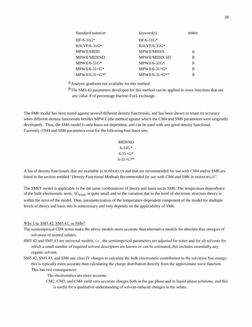
38

Standard notation keyword(s) notes

HF/6-31G* HF/6-31G*

B3LYP/6-31G* B3LYP/6-31G*

MPWX/MIDI! MPWX/MIDIX a

MPWX/MIDI!6D MPWX/MIDIX 6D b

MPWX/6-31G* MPWX/6-31G* b

MPWX/6-31+G* MPWX/6-31+G* b

MPWX/6-31+G** MPWX/6-31+G** b

aAnalytic gradients not available for this method.

bThe SM5.43 parameters developed for this method can be applied to wave functions that use

any value X of percentage Hartree-Fock exchange.

The SM6 model has been tested against several different density functionals, and has been shown to retain its accuracy

when different density functionals besides MPWX (the method against which the CM4 and SM6 parameters were originally

developed). Thus, the SM6 model is only basis-set-dependent, and can be used with any good density functional.

Currently, CM4 and SM6 parameters exist for the following four basis sets:

MIDI!6D

6-31G*

6-31+G*

6-31+G**

A list of density functionals that are available in HONDOPLUS and that are recommended for use with CM4 and/or SM6 are

listed in the section entitled “Density Functional Methods Recommended for use with CM4 and SM6 in HONDOPLUS”.

The SM6T model is applicable to the the same combinations of theory and basis set as SM6. The temperature dependence

of the bulk-electrostatic term, GENP, is quite small and so the variation due to the level of electronic structure theory is

within the error of the model. Thus, parameterization of the temperature-dependent component of the model for multiple

levels of theory and basis sets is unnecessary and only depends on the applicability of SM6.

Why Use SM5.42, SM5.43, or SM6?

The semiempirical CDS terms make the above models more accurate than alternative models for absolute free energies of

solvation of neutral solutes.

SM5.42 and SM5.43 are universal models, i.e., the semiempirical parameters are adjusted for water and for all solvents for

which a small number of required solvent descriptors are known or can be estimated; this includes essentially any

organic solvent.

SM5.42, SM5.43, and SM6 use class IV charges to calculate the bulk electrostatic contribution to the solvation free energy;

this is typically more accurate than calculating the charge distribution directly from the approximate wave function.

This has two consequences:

The electrostatics are more accurate.

CM2, CM3, and CM4 yield very accurate charges both in the gas phase and in liquid-phase solutions, and this

is useful for a qualitative understanding of solvent-induced changes in the solute.

39

SM5 and SM6 parameterizations included an extremely broad range of solute functional groups, including molecules

containing phosphorus, which are very hard to treat.

SM5 and SM6 do not need to be corrected for outlying charge error, which can be large in some other methods.

Furthermore, our most recent model, SM6, has several advantages compared to earlier solvent models (e.g.

SM5.42 and SM5.43) developed within our group:

SM6 can be used with any of the density functional methods supported in HONDOPLUS. For a list of recommended density

functional methods that are supported in HONDOPLUS, see the section entitled “Density Functional Methods

Recommended for use with CM4 and SM6 in HONDOPLUS”.

SM6 significantly outperforms SM5.42, SM5.43, as well as all other competing continuum solvation models that it has

been tested against for predicting aqueous solvation free energies of ions. This is important because aqueous solvation

free energies of ions can be used in various thermodynamic cycles to calculate pKa.

When explicit water molecules are added to the calculation (which is sometimes required for accurately calculating aqueous

solvation free energies of some solutes, in particular ions with concentrated regions of charge) the performance of SM6

signficantly improves, whereas the performance of SM5.42, SM5.43, and most other competing continuum solvation

models that SM6 has been tested against worsens. Thus, unlike other popular continuum solvation models, SM6 can

be applied to solute-water clusters.

SM6 uses an improved set of surface tension functionals; using this new set of surface tension functionals significantly

improves the performance of the model for molecules containing peroxide functional groups.

SM6 uses class IV CM4 charges, which give more realistic partial atomic charges for aliphatic groups than our previous

class IV models; this is important for accurately modeling hydrophobic effects.

Why Use SM6T?

SM6T is one of the few implicit models capable predicting aqueous free energies of solvation as a function of temperature.

SM6T has been tested against a much broader range of compounds than prior models.

SM6T is based on a very well tested solvation models and so shares in the positive aspects of this models, as described

above and uses a physically reasonable approach to parameterize the temperature dependent component of the model.

Notation

The following notation is recommended:

Geometry optimized at level X/Y in the gas phase, followed by a single-point SMx solvation calculation at level W/Z,

where W/Z is one of the choices supported by ICMD:

SMx/W/Z/ /X/Y

If X/Y is the same as W/Z, then / /X/Y may be substituted by //g,, where g denotes gas-phase:

SMx/W/Z//g

Previously, solvation calculations carried out using gas-phase geometries were denoted by including an “R”

suffix after the name of the SMx model. Here, this older notation has been replaced with the notation above.

For a liquid-phase geometry optimization the //X/Y is dropped, and this calculation is denoted as follows:

40

SMx/W/Z

Previously, solvation calculations carried out using liquid-phase geometries were denoted by dropping the “R”

suffix after the name of the SMx model. Here, we drop this suffix for all solvation calculations and use the

notation described above.

SCRF calculations using generalized Born model and CM2, CM3, or CM4 charges

A self-consistent-reaction-field method based on the generalized Born approximation and CM2, CM3, or CM4 charges has

been implemented in the program. One can use the SCRF orbitals to calculate polarization and distortion energies and

solvated atomic partial charges and to investigate solvation effects on the atomic charge distribution, multipole moments,

and other one-electron properties. In addition, the SCRF calculation can be used to calculate the free energy of solvation.

Note that in SMx models, the GB calculation is one of two components of the solvation energy (the other being based on

solvent-accessible surface areas), but in the GB model it is the only component. As a consequence, GB calculations are

more sensitive to the atomic radii (Coulomb radii) than are SMx calculations.

Solvent-accessible surface area and solvation free energy in aqueous and organic solutions

The calculation of free energies of solvation by SMx models requires that one add the so-called CDS term to the

polarization energy and the distortion energy. In particular, the standard-state free energy of solvation is given by eq. (1)

where GCDS is the specific contribution from short-range effects associated primarily with the first solvation shell.

Calculation of GCDS is based on the Analytic Surface Area (ASA) algorithm. Both SM5.42 and SM5.43 can be used to

calculate solvation free energies in aqueous solution and organic-solvent solutions. Currently, SM6 and SM6T are

parametrized for aqueous solvent only.

Literature references of the solvation models, charge models, electronic structure methods, and basis sets

ASA algorithm

LH95 Liotard, D. A; Hawkins, G. D.; Lynch, G. C.; Cramer, C. J.; Truhlar, D. G. “Improved Methods for Semiempirical

Solvation Models” J. Comp. Chem. 1995, 16, 422.

MIDI! Basis set

EG96 Easton, R. E.; Giesen, D. J.; Welch, A.; Cramer, C. J.; Truhlar, D. G. “The MIDI! Basis Set for Quantum

Mechanical Calculations of Molecular Geometries and Partial Charges” Theor. Chim. Acta 1996, 93, 281.

LC98 Li, J.; Cramer, C. J.; Truhlar, D. G. “MIDI! Basis Set for Silicon, Bromine, and Iodine” Theor. Chem. Acc. 1998,

99, 192.

TW01 Thompson, J. D.; Winget, P.; Truhlar, D. G. “MIDIX basis set for the lithium atom: Accurate geometries and

partial atomic charges with minimal computational cost”, PhysChemComm, 2001, 4, 72.

41

Corrected modified Perdew-Wang hybrid DFT method

LZ03 Lynch, B. J.; Zhao, Y.; Truhlar, D. G. “The Effectiveness of Diffuse Basis Functions for Calculating Relative

Energies by Density Functional Theory”, J. Phys. Chem. A 2003, 107, 1384.

42

MPW1K

LF00 Lynch, B. J.; Fast, P. L.; Harris, M.; Truhlar D. G. “Adiabatic Connection for Kinetics”, J. Phys. Chem. A 2000,

104, 4811.

MPWPW91, mPW1PW91, and MPWX

AB98 Adamo, C.; Barone, V.; “Exchange functionals with Improved Long-Range Behavior and Adiabatic Connection

Methods without Adjustable Parameters: The mPW and mPW1PW Models” J. Chem. Phys. 1998, 108, 664.

PT02 Pu, J.; Truhlar, D. G. “Parameterized Direct Dynamics Study of Rate Constants of H with CH4 from 250 to

2400K”, J. Chem. Phys. 2002, 116, 1468.

Löwdin population analysis

LD50 Löwdin, P. –O. J. Chem. Phys. 1950, 18, 365. (b) Del Re, G.; In Quantum Science; Calais, J. –L., Goscinski, O.,

Linderberg, J., Öhrn, Y., Eds.;Plenum Press: New York, 1976; p 53.

Redistributed Löwdin population analysis

TX02 Thompson, J. D.; Xidos, J. D.; Sonbuchner, T. M.; Cramer, C. J.; Truhlar, D. G. “More Reliable Partial Atomic

Charges when using Diffuse Basis Sets”, PhysChemComm, 2002, 5, 117.

Original parameterizations of the CM2 Charge Model

LZ98 Li, J.; Zhu, T.; Cramer, C. J.; Truhlar, D. G. “A New Class IV Charge Model for Extracting Accurate Partial

Charges from Wave Functions” J. Phys. Chem. A 1998, 102, 1820.

Parameterization of the CM2 model for HF/cc-pVDZ

LX99 Li, J.; Xing, J.; Cramer, C. J.; Truhlar, D. G. “Accurate Dipole Moments from Hartree-Fock Calculations by

Means of Class IV Charges” J. Chem. Phys. 1999, 111, 885.

Original parameterizations of the CM3 Charge Model

WT02 Winget, P.; Thompson J. D.; Xidos, J. D.; Cramer, C. J.; Truhlar, D. G. “Charge Model 3: A Class IV Charge

Model based on Hybrid Density Functional Theory with Variable Exchange” J. Phys. Chem. A, 2002, 106, 10707.

Extension of CM3 to AM1, PM3, BLYP, and B3LYP

TC03 Thompson, J. D.; Cramer, C. J.; Truhlar, D. G. “Parameterization of Charge Model 3 For AM1, PM3, BLYP, and

B3LYP” J. Comput. Chem., 2003, 24, 1291.

43

Extension of CM3 and CM3.1 to HF/MIDI!

KC05a Kelly, C. P.; Cramer, C. J.; Truhlar, D. G. “Accurate Partial Atomic Charges for High-Energy Molecules with the

MIDI! Basis Set” Theor. Chem. Acc., 2005, 113, 133.

Parameterizations of the CM4 Charge Model

KC05b Kelly, C. P.; Cramer, C. J.; Truhlar, D. G. “SM6: A Density Functional Theory Continuum Solvation Model for

Calculating Aqueous Solvation Free Energies of Neutrals, Ions, and Solute-Water Clusters” J. Theor. Comput.

Chem 2005, 1, 1133.

SM5.42/DFT method and ISCRF=1 option

ZL98 Zhu, T.; Li, J.; Hawkins, G. D.; Cramer, C. J.; Truhlar, D. G. “Density Functional Solvation Model Based on CM2

Atomic Charges” J. Chem. Phys. 1998, 109, 9117.

SM5.42/MIDI!6D method and more efficient version of ISCRF=1 option

LH98 Li, J.; Hawkins, G. D.; Cramer, C. J.; Truhlar, D. G. “Universal Reaction Field Model Based on Ab Initio Hartree-

Fock Theory” Chem. Phys. Lett. 1998, 288, 293.

Additional SM5.42 parameterizations and ISCRF=2 option

LZ99 Li, J.; Zhu, T.; Hawkins, G. D.; Winget, P.; Liotard, D. A.; Cramer, C. J.; Truhlar, D. G. “Extension of the

Platform of Applicability of the SM5.42R Universal Solvation Model” Theor. Chem. Acc. 1999, 103, 9.

SM5.42 parameterization for Si

WT02 Winget, P.; Thompson, J. D.; Cramer, C. J.; Truhlar, D. G. “Parameterization of a Universal Solvation Model for

Molecules Containing Silicon” J. Phys. Chem. B, 2002, 106, 5160.

Parameterization of SM5.42 for soil

WC00 Winget, P.; Cramer, C. J.; Truhlar, D. G. “Prediction of Soil Sorption Coefficients Using a Universal Solvation

Model” Env. Sci. Technol. 2000, 34, 4733.

SM5.43 parameterizations for HF/6-31G*, B3LYP/6-31G*, mPW1PW91/6-31G*, and mPW1PW91/6-31+G*

TC04 Thompson, J. D.; Cramer, C. J.; Truhlar, D. G. “New Universal Solvatoin Model and Comparison of the Accuracy

of the SM5.42R, SM5.43R, C-PCM, D-PCM, and IEF-PCM Continuum Solvation Models for Aqueous and

Organic Solvation Free Energies and Vapor Pressures” J. Phys. Chem. A 2004, 108, 6532.

SM5.43 parameterizations for MPWX/MIDIX, MPWX/MIDI!6D, MPWX/6-31G*, MPWX/6-31+G*, and MPWX/6-

31+G**

TC05 Thompson, J. D.; Cramer, C. J.; Truhlar, D. G. “Density-Functional Theory and Hybrid Density-Functional Theory

Continuum Solvation Models for Aqueous and Organic Solvents: Universal SM5.43 and SM5.43R Solvation

Models for Any Fraction of Hartree-Fock Exchange” Theor. Chem. Acc. 2005, 113, 107.

44

SM6 aqueous model

KC05b Kelly, C. P.; Cramer, C. J.; Truhlar, D. G. “SM6: A Density Functional Theory Continuum Solvation Model for

Calculating Aqueous Solvation Free Energies of Neutrals, Ions, and Solute-Water Clusters” J. Theor. Comput.

Chem 2005, 1, 1133.

SM6T aqueous model

AC06 Chamberlin, A. C.; Cramer, C. J.; Truhlar, D. G. “Predicting Free Energies of Solvation as Functions of

Temperature” J. Phys. Chem. A. 2006 In Press.

Analytical gradients of the SM5.42, SM5.43, and SM6 models

ZL99 Zhu, T.; Li, J.; Liotard, D. A.; Cramer, C. J.; Truhlar, D. G. “Analytical Gradients of a Self-Consistent Reaction-

Field Solvation Model Based on CM2 Atomic Charges” J. Chem. Phys. 1999, 110, 5503.

Overview article including SM5.42

HZ99 Hawkins, G. D.; Zhu, T.; Li, J.; Chambers, C. C.; Giesen, D. J.; Liotard, D. A.; Cramer, C. J.; Truhlar, D. G.

“Universal Solvation Models” in Combined Quantum Mechanical and Molecular Mechanical Methods, Gao, J.,

Thompson, M. A., Eds.; American Chemical Society: Washington DC; 1998; pp. 201-219.

Sample applications of SM5.42

TC98 Truhlar, D. G.; Cramer, C. J. “Solvent Effects on 1,3-Dipolar Addition Reactions” Faraday Discussions 1998,

110, 477.

LC99 Li, J.; Cramer, C. J.; Truhlar, D. G. “Application of a Universal Solvation Model to Nucleic Acid Bases.

Comparison of Semiempirical Molecular Orbital Theory, Ab Initio Hartree-Fock Theory, and Density Functional

Theory” Biophys. Chem. 1999, 78, 147.

WH00 Winget, P.; Hawkins, G. D.; Cramer, C. J.; Truhlar, D. G. “Prediction of Vapor Pressures from Self-Solvation Free

Energies Calculated by the SM5 Series of Universal Solvation Models” J. Phys. Chem. B, 2000, 104, 4726.

WW00 Winget, P.; Weber, E. J.; Cramer, C. J.; Truhlar, D. G. “Computational Electrochemistry: Aqueous Oxidation

Potentials for Substituted Anilines,” Phys. Chem. Chem. Phys., 2000, 2, 1231.

CR99 Chuang, Y.-Y.; Radhakrishnan, M. L.; Fast, P. L.; Cramer, C. J.; Truhlar, D. G. “Direct Dynamics for Free Radical

Kinetics in Solution: Solvent Effect on the Rate Constant for the Reaction of Methanol with Atomic Hydrogen” J.

Phys. Chem. A 1999, 103, 4893.

ST01 Sicinska, D.; Truhlar, D. G.; Paneth, P. “Solvent-Dependent Transition states for Decarboxylations”, J. Am. Chem.

Soc. 2001, 123, 7863.

SP02 Sicinska, D.; Paneth, P.; Truhlar, D. G. “How Well Does Microsolvation Represent Macrosolvation? A Test case:

Dynamics of Decarboxylation of 4-Pyridylacetic Acid Zwitterion” J. Phys. Chem. B 2002, 106, 2708.

45

Quick index to literature

The references for the methods supported by MN-GSM-v5.2 are as follows:

Method Reference

Löwdin charges LD50

RLPA charges TX02

mPW hybrid functional AB98, PT02 and LZ03

MPW1K LF00

MPWX PT02

CM2/HF/MIDI! LZ98

CM2/HF/MIDI!6D LZ98

CM2/HF/6-31G* LZ98

CM2/BPW91/MIDI! LZ98

CM2/BPW91/MIDI!6D LZ98

CM2/B3LYP/MIDI! LZ98

CM2/BPW91/6-31G* LZ98

CM2/HF/6-31+G* LZ98

CM2/HF/cc-pVDZ LX99

CM2/BPW91/DZVP LZ98

CM3/HF/MIDI! KC05a

CM3/HF/MIDI!6D WT02

CM3/HF/6-31G* WT02

CM3/MPWX/MIDI! WT02

CM3/MPWX/MIDI!6D WT02

CM3/MPWX/6-31G* WT02

CM3/MPWX/6-31+G* WT02

CM3/MPWX/6-31+G** WT02

CM3/BLYP/6-31G* TC03

CM3/B3LYP/MIDI!6D TC03

CM3/B3LYP/6-31G* TC03

CM3/B3LYP/6-31+G* TC03

CM3.1/HF/MIDI! KC05a

CM4/DFT/MIDI!6D KC05b

CM4/DFT/6-31G* KC05b

CM4/DFT/6-31+G* KC05b

CM4/DFT/6-31+G** KC05b

SM5.42/HF/MIDI! LZ99

SM5.42/HF/MIDI!6D LH98

SM5.42/HF/6-31G* LZ99

SM5.42/BPW91/MIDI! LZ99

SM5.42/BPW91/MIDI!6D ZL98

SM5.42/B3LYP/MIDI! LZ99

SM5.42/BPW91/6-31G* ZL98

SM5.42/HF/6-31+G* LZ99

SM5.42/HF/cc-pVDZ LZ99

SM5.42/BPW91/DZVP ZL98

SM5.43/HF/6-31G* TC04

SM5.43/B3LYP/6-31G* TC04

SM5.43/MPWX/MIDI! TC05

SM5.43/MPWX/MIDI!6D TC05

SM5.43/MPWX/6-31G* TC05

46

SM5.43/MPWX/6-31+G* TC05

SM5.43/MPWX/6-31+G** TC05

SM6/DFT/MIDI!6D KC05b

SM6/DFT/6-31G* KC05b

SM6/DFT/6-31+G* KC05b

SM6/DFT/6-31+G** KC05b

SM6T/DFT/MIDI!6D AC06

SM6T/DFT/6-31G* AC06

SM6T/DFT/6-31+G* AC06

SM6T/DFT/6-31+G** AC06

SM5.42, SM5.43, and SM6 liquid-

phase optimizations

ZL99 and CR99

47

Usage of the solvation models

HONDO and HONDOPLUS input options are discussed in detail later in this manual. This section contains additional

information for HONDOPLUS users.

As discussed at length above, input for HONDO consists of a series of NAMELIST and DATA entries that can be entered in

any order in the input file (with a few exceptions, see AIX, IRIX, and Linux Implementations). It should be noted that all

namelist and data input statements must be preceeded by a single blank space. To run a CM2, CM3, SM5.42R, SM5.42,

SM5.43R, SM5.43, or generalized Born calculation, the following namelist and data groups must be defined in the input

file:

$CTL, to specify the type of calculation (single-point energy, single-point energy plus gradient, etc.), the wave

function and the type of algorithm to use for storing the two-electron integrals. The type of calculation is

requested with the 'RUNFLG' keyword. For a single-point energy calculation, which can be used to carry out a

Löwdin population analysis, an RLPA calculation, a CM2, CM3, or CM4 calculation, a calculation with the

generalized Born method, or an single-point SMx (x = 5.42, 5.43, or 6) calculation, RUNLFG should be set to 0.

For a calculation of the energy and the gradient with the generalized Born method or with the SM5.42, SM5.43, or

CM6 method, RUNFLG should be set to -3. For geometry optimizations to a minimum or to a first order saddle

point, RUNFLG should be set to 1 or 3, respectively. Finally, to compute the Hessian with the generalized Born

model, SM5.42, SM5.43, or with SM6, RUNFLG should be set to 2. Another important keyword in this namelist

is the 'DIRECT' keyword. This keyword determines which type of algorithm to use to store the two-electron

integrals. By default, HONDOPLUS uses a conventional algorithm, i.e., the integrals are calculated once for a given

SCF calculation, stored on disk, and retrieved from disk as needed. This is a logical choice for most calculations.

However, for versions of HONDOPLUS that are compiled on 32-bit machines, the user may run into problems with

file size limits. In this case, the DIRECT keyword should be set to 1 for a direct algorithm or 2 for a semi-direct

algorithm. The DIRECT=1 option requests that the two-electron integrals are calculated as needed, so none of

them are stored on disk. The DIRECT=2 option requests to store some of the two-electron integrals on disk, but

not all of them. This latter option works with some other options in the $INTGRL namelist, which is fully

described later on in the manual. Note that the direct algorithms (DIRECT=1 or DIRECT=2) are not supported for

DFT calculations yet.

$BAS, to specify the basis set to use in the calculation. For example, to carry out a calculation by HF/6-31G* (for

molecules that do not contain iodine), the $BAS data group would be:

$BAS 6-31G* $END

or

$BAS 6-31GA* $END

In addition, a general basis set (i.e., a basis set not stored internally in the HONDOPLUS code) can be entered; in this

case, the basis set for every atom in the molecular species must be specified in order. Samples S1 and S3 provide

examples of this. The files midi-bang.bas, 6-31GS.bas, 6-31PGS.bas, 6-31PGSS.bas, ccpVDZ.bas, and dzvp.bas are

provided in the ‘hondoplus-v5.2/HondoS/Input’ directory for the users’ convenience. These files contain the MIDI!,

6-31G*, 6-31+G*, 6-31+G**, cc-pvDZ, and DZVP basis sets, respectively, in HONDO/HONDOPLUS input format. The

section entitled Special notes on basis sets provides more details on the makeup of these basis sets. Note that

keywords exist to request calculations with the 6-31G* and MIDI! basis sets. Further examples of general basis set

input are available in the test suite input files that are also located in the ‘hondoplus-v5.2/HondoS/Input’ directory.

48

$GEO, for defining the geometry of the molecule. The first line after the $GEO statement is a title line. This is

followed by specifying the geometry of the molecule using either Cartesian coordinates or a Z-matrix. Cartesian

and Z-matrix input is free format. Cartesian input is in the form “atom label x-coordinate y-coordinate z-

coordinate”, where the coordinates are in angstroms. The form of the Z-matrix is described in detail in the section

entitled Data group $GEO. The atom labels for both Cartesian and Z-matrix input must consist of the atomic

symbols, optionally followed by a character string that must start with a number. Inputting atomic numbers as

atom labels is not supported by HONDO.

In addition to these data groups, one of the following namelists must also be defined in the input:

$HONDOS, $CM2, or $SM5 for specifying various options for a CM2, CM3, or an SMx (x = 5.42, 5.43, 6 or 6T)

calculation. These namelists all define the same input parameters for a HONDOPLUS calculation, but only one of

them should be defined in the input file. If more than one of these namelists are defined in an input file, the input

options defined in the other namelists will be ignored. The section entitled Namelists $HONDOS, $CM2, and

$SM5 provides details for the various options available. Although default values exist for all keywords, the user

should take care in setting ISCRF, ICMD, and IAQU. If an organic solvent is used (IAQU = 0), the user should

input as many solvent descriptors that are available for that particular solvent. For a given solvent, these values

can be derived from experiment or from interpolation or extrapolation of data available for other solvents. Solvent

parameters for common organic solvents are tabulated in the Minnesota Solvent Descriptor Database. Links to the

latest version of this database is available at: http://comp/chem.umn.edu/hondoplus. This version of HONDOPLUS

also assumes that the input geometry for a geometry optimization in solution is already the gas-phase optimum

geometry.

To run a CM2, CM3, CM4 an SMx (x = 5.42, 5.43, 6 or 6T), or a GB calculation using a DFT or hybrid DFT wave

function, the $SCF namelist is required. The DFTFLG keyword must be set equal to 1 to indicate that a DFT

wave function is to be employed. The DFTFUN keyword must also be set to the integer value that is assigned to

the desired DFT wave function. CM2 and SM5.42 currently support B3LYP (DFTFUN=6) and BPW91

(DFTFUN=7) wave functions, CM3 and SM5.43 supports MPWX hybdrid DFT (DFTFUN=8 for MPW1K, 9 for

mPW1PW91, and 3X for MPWX, where X/10 is the percentage of HF exchange in the mPW functional), and CM4

and SM6 support any of the density functional methods available in HONDOPLUS, along with the following basis

sets: MIDI!6D, 6-31G(d), 6-31+G(d), and 6-31+G(d,p). A full listing of available DFT wave functions are

provided in the Namelist $SCF section, and those DFT methods recommended for use with CM4 and SM6 are

given in the section entitled “Density Functional Methods Recommended for use with CM4 and SM6 in

HONDOPLUS”. The grid used for DFT calculations can be adjusted using the $DFT namelist.

Some other useful input options are available in the $SCF namelist, in particular, MAXIT = X and ACURCY = Y. The

option MAXIT sets the maximun number of SCF and SCRF cycles to X (default is 30), and the ACURCY option sets the

convergence on the density matrix to be Y (default is 0.00001).

To run an SM5.42, SM5.43, or SM6 geometry optimization in solution, the $OPT namelist may also be defined. This

namelist controls the convergence threshold on the maximum component of the gradient with the CVGOPT keyword

(default = 0.0005), the maximum number of energy calculations allowed with the NPTOPT keyword (default = 50), and

what type of Hessian is initially used with the INHESS keyword (default is to use 0.5*unit matrix). We have tested

geometry optimizations in solution with analytical gradients for a number of simple cases and have found no trouble when

using the default Hessian. However, for saddle point optimizations, we have found that using the default initial Hessian

never leads to a first order saddle point. We therefore suggest that saddle point optimizations should either not be

attempted with SM5.42, SM5.43, and SM6, or that an initial Hessian is calculated and used for a subsequent saddle point

optimization. Note that at this time SM6T cannot be used in combination with geometry optimization.

49

Examples of HONDOPLUS input and output for the solvation models are presented in Sample S1, S2, and S3 and in the test

suite located in the ‘hondoplus-v5.2/HondoS’ directory.

HONDOPLUS is executed with the following command line:

/directory/hondoplus-v5.2/master/hondo.x input_file output_file

where directory is the UNIX path to the HONDOPLUS distribution directory and input_file and output_file are the

HONDOPLUS input and output files, respectively. Alternatively, if the user executes

/directory/hondoplus-v5.2/master/hondo.x with no other input, the program will ask the user for an input and an output file

name.

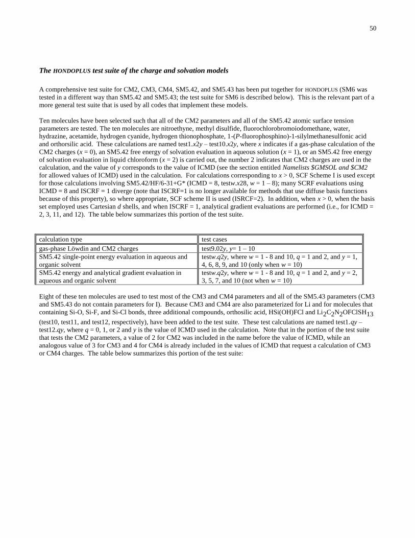
50

The HONDOPLUS test suite of the charge and solvation models

A comprehensive test suite for CM2, CM3, CM4, SM5.42, and SM5.43 has been put together for HONDOPLUS (SM6 was

tested in a different way than SM5.42 and SM5.43; the test suite for SM6 is described below). This is the relevant part of a

more general test suite that is used by all codes that implement these models.

Ten molecules have been selected such that all of the CM2 parameters and all of the SM5.42 atomic surface tension

parameters are tested. The ten molecules are nitroethyne, methyl disulfide, fluorochlorobromoiodomethane, water,

hydrazine, acetamide, hydrogen cyanide, hydrogen thionophosphate, 1-(P-fluorophosphino)-1-silylmethanesulfonic acid

and orthorsilic acid. These calculations are named test1.x2y – test10.x2y, where x indicates if a gas-phase calculation of the

CM2 charges (x = 0), an SM5.42 free energy of solvation evaluation in aqueous solution (x = 1), or an SM5.42 free energy

of solvation evaluation in liquid chloroform (x = 2) is carried out, the number 2 indicates that CM2 charges are used in the

calculation, and the value of y corresponds to the value of ICMD (see the section entitled Namelists $GMSOL and $CM2

for allowed values of ICMD) used in the calculation. For calculations corresponding to x > 0, SCF Scheme I is used except

for those calculations involving SM5.42/HF/6-31+G* (ICMD = 8, testw.x28, w = 1 – 8); many SCRF evaluations using

ICMD = 8 and ISCRF = 1 diverge (note that ISCRF=1 is no longer available for methods that use diffuse basis functions

because of this property), so where appropriate, SCF scheme II is used (ISRCF=2). In addition, when x > 0, when the basis

set employed uses Cartesian d shells, and when ISCRF = 1, analytical gradient evaluations are performed (i.e., for ICMD =

2, 3, 11, and 12). The table below summarizes this portion of the test suite.

calculation type test cases

gas-phase Löwdin and CM2 charges test9.02y, y= 1 – 10


organic solvent


4, 6, 8, 9, and 10 (only when w = 10)




3, 5, 7, and 10 (not when w = 10)

Eight of these ten molecules are used to test most of the CM3 and CM4 parameters and all of the SM5.43 parameters (CM3

and SM5.43 do not contain parameters for I). Because CM3 and CM4 are also parameterized for Li and for molecules that

containing Si-O, Si-F, and Si-Cl bonds, three additional compounds, orthosilic acid, HSi(OH)FCl and Li2C2N2OFClSH13

(test10, test11, and test12, respectively), have been added to the test suite. These test calculations are named test1.qy –

test12.qy, where q = 0, 1, or 2 and y is the value of ICMD used in the calculation. Note that in the portion of the test suite

that tests the CM2 parameters, a value of 2 for CM2 was included in the name before the value of ICMD, while an

analogous value of 3 for CM3 and 4 for CM4 is already included in the values of ICMD that request a calculation of CM3

or CM4 charges. The table below summarizes this portion of the test suite:

51

Nine of these tem molecules (CM3 and SM5.43 parameters are not available for iodine) are used to test most of the CM3

and CM4 parameters and all of the SM5.43 parameters. Because CM3 is also parameterized for Li and for molecules that

contain Si-O, Si-F, and Si-Cl bonds, two additional compounds, HSi(OH)FCl and Li2C2N2OFClSH13 (test11 and test12,

respectively) are used. These test calculations are named test11.x.qy – test12.x.qy, where x is the percentage of HF

exchange used in MPWX multiplied by 10 (e.g., MPW42.8 corresponds to x = 428), the q is 0 to indicate a gas-phase

calculation, 1 to indicate a calculation in water, and 2 to indicate a calculation in an organic solvent, and y indicates the

value of ICMD. For the HF/MIDI!6D and HF/6-31G* parameter sets, the test calculations are named test1.HF.qy –

test12.HF.qy, for y = 302 and 303. For BLYP and B3LYP, the CM3 test calculations are named test1.qy – test12.qy, where

y = 313, 314, 320, and 321. Note that in the portion of the test suite that tests the CM2 parameters, a value of 2 for CM2

was included in the name before the value of ICMD, while an analogous value of 3 for CM3 is already included in the

values of ICMD that request a calculation of CM3 charges. The table below summarizes the part of the test suite that tests

the CM3 and SM5.43 parameters:

calculation type test case names

gas-phase Löwdin and CM3 charges by MPWX testw.x.0y, where w = 1, 2, 4 - 12, x = 0, 25, 428, 517,

606, and 999, and y = 315, 316, and 317

gas-phase RLPA and CM3 charges by MPWX testw.x.0y, where w = 1, 2, 4 - 12, x = 0, 25, 428, 517,

606, and 999, and y = 318 and 319

gas-phase CM3 charges by BLYP and B3LYP test.w.0y, where w = 1, 2, 4- 12, y = 320 and 321

gas-phase RLPA and CM3 charges by B3LYP/6-31+G* testw.0314, where w = 1, 2, 4 - 12

gas-phase Löwdin and CM3 charges by HF testw.HF.0301, where w = 1, 2, 4 - 12

testw.HF.0302, where w = 1, 2, 4 - 12

testw.HF.0303, where w = 1, 2, 4 - 12


999, and y = 416 and 417


999, and y = 418 and 419

gas-phase Löwdin and CM3.1 charges by HF/MIDI! testw.HF.0322, where w = 1, 4, 5, 6, and 7



testw.x.y, where w = 1, 2, 4 - 8, x = 0, 25, 428, 517, and

606, and y = 1316, 1317, 2316, and 2317

testw.y, where w = 1, 2, 4 - 8 and y = HF.1303, 1313,

2303, and 2313


organic solvent

testw.x.0y, where w = 1, 2, 4 - 8, x = 0, 25, 428, 517, and

606, and y = 1315, 1317, 1318, 1319, 2315, 2317, 2318,

and 2319

52

The remaining test jobs test the remaining keywords available in HONDOPLUS:

Two test calculations are performed using SM5.42/HF/MIDI!6D (ISCRF = 1):

geometry optimization of 2,4-pentadione in acetonitrile solution (test13).

transition state optimization for the SN2 reaction of NH3 and CH3Cl in aqueous solution (the Menschutkin reaction;

test14b). Two numerical Hessian calculations are carried out: test14a generates a Hessian using forward

differences that is required for the transition state optimization in test14b and test14c generates a more accurate

Hessian using central differences to ensure that the stationary-point is a first-order saddle point via vibrational

frequency analysis.

Test case test16a performs a Generalized Born electrostatic solvation energy and gradient evaluation using Löwdin partial

atomic charges and UHF/6-31G(df) for the peroxide radical in aqueous solution. Test16a also tests the use of Cartesian f

functions and unrestricted wave functions. Test16b evaluates the free energy of solvation for HOO– in water using

GB/RHF/MG3 to test the use of spherical harmonic d and f functions

Test cases test17a tests the ICSAVE = 1 option, while test17b tests the ICREAD = 1 option. The CM2 charges calculated

in test17a are written to a file, CM2CHG. The charges in file CM2CHG are read in and used in test17b. Both test cases

perform an SM5.42R/HF/MIDI!6D calculation of water solute in acetone solvent, using ISCRF = 2, and both produce the

same energetic results.

HONDOPLUS versions up to and including version 3.1 did not evaluate the Mayer bond order matrix correctly for

unrestricted wave functions (see Revision History for HONDOPLUS version 3.1.1 for more details). Test case test20 was

added to illustrate the correct evaluation of the Mayer bond order, CM2 charges, solvation energy, and gradient for an

unrestricted wave function that yields results that are significantly different from those obtain when using HONDOPLUS

versions up to 3.1. The calculation is for

CH4+in water solvent using SM5.42/UHF/6-31G* level of theory.

Test cases test21, test22, test23, and test26 test the MPWX method. Test case test21 is a geometry optimization of diatomic

Li by mPW1PW91/6-311G*. Test case test22 is a geometry optimization of the hydroxyl radical by

mPW1PW91/6-311G**. Test case test23 is a geometry optimization of the hydroxyl radical by mPW1PW91/6-31G*. Test

case test26 is a single point energy calculation of hydroxyl radical by MPW1K/6-31G**. Test cases test24 and test25 test

the DFTFUN keyword (defined in the $SCF namelist), which allows for specification of an arbitrary percentage of HF

exchange in all DFT methods available in HONDO. Test case test24 tests the DFTFUN keyword for BH&HLYP, while test

case test25 tests the DFTFUN keyword for BPW91.

Test case test27 tests the calculation of the electrostatic contribution to the aqueous free energy of solvation of water using

RLPA charges. In addition, the corresponding free energy gradient is also calculated.

The CM3 model has been extended to the BLYP and B3LYP methods for several basis sets (ICMD = 313, 314, 320, and

321). The CM3 model for these methods uses a new charge-mapping scheme for compounds that contain N and O. To test

the new mapping scheme, test case test28 has been added to the test suite. In test28, the electrostatic contribution to the

aqueous free energy of solvation of pyramidal-formamide using CM3 charges calculated by B3LYP/6-31G* are calculated.

An analytical gradient calculation is also carried out in test28.

The SM6 model uses a new surface tension for oxygen atoms. This new surface tension is tested in test29 and test30.

The SM6T model uses three new keywords SolK, ReadK, and AvgK. The the two molecules used for testing the SM6T

keywords, 2-propanol and furfural, were selected to show the variability of the electrostatic contribution to the free energy

of solvation and to test the available surface tension parameters. The calculations were performed using the MPW<Blank>

level of theory. The tests are denoted test31.xy, test32y and test33y. (x denotes the temperatures at which the calculation

was performed 273, 298, 348, 373 K and y denotes the compounds 2-propanol, a, and furfural, b.) The SM6T model uses

three new keywords SolK, ReadK, and AvgK. SolK is tested in the test set test31.xy. The ReadK option is tested in the pair

of tests labeled test32x. The AvgK option is tested tested in the pair of tests labeled test33x

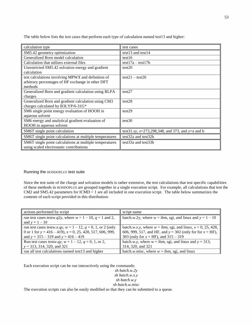
53

The table below lists the test cases that perform each type of calculation named test13 and higher:

calculation type test cases

SM5.42 geometry optimization test13 and test14

Generalized Born model calculation test16

Calculation that utilizes external files test17a – test17b

Unrestricted SM5.42 solvation energy and gradient

calculation

test20

test calculations involving MPWX and definition of

arbitrary percentages of HF exchange in other DFT

methods

test21 – test26

Generalized Born and gradient calculation using RLPA

charges

test27

Generalized Born and gradient calculation using CM3

charges calculated by B3LYP/6-31G*

test28

SM6 single point energy evaluation of HOOH in

aqueous solvent

test29

SM6 energy and analytical gradient evaluation of

HOOH in aqueous solvent

test30

SM6T single point calculation test31.xy, x=273,298,348, and 373, and y=a and b


SM6T single point calculations at multiple temperatures

using scaled electrostatic contributions

test33a and test33b

Running the HONDOPLUS test suite

Since the test suite of the charge and solvation models is rather extensive, the test calculations that test specific capabilities

of these methods in HONDOPLUS are grouped together in a single execution script. For example, all calculations that test the

CM2 and SM5.42 parameters for ICMD = 1 are all included in one execution script. The table below summarizes the

contents of each script provided in this distribution:

actions performed by script script name

run test cases testw.q2y, where w = 1 – 10, q = 1 and 2,

and y = 1 – 10

batch.w.2y, where w = ibm, sgi, and linux and y = 1 – 10

run test cases testw.x.qy, w = 1 – 12, q = 0, 1, or 2 (only

0 or 1 for y = 416 – 419), x = 0, 25, 428, 517, 606, 999,

and y = 315 – 319 and y = 416 – 419

batch.w.x.y, where w = ibm, sgi, and linux, x = 0, 25, 428,

606, 999, 517, and HF, and y = 302 (only for for x = HF),

303 (only for x = HF), and 315 – 319

Run test cases testw.qy, w = 1 – 12, q = 0, 1, or 2,

y = 313, 314, 320, and 321

batch.w.y, where w = ibm, sgi, and linux and y = 313,

314, 320, and 321

run all test calculations named test13 and higher batch.w.misc, where w = ibm, sgi, and linux

Each execution script can be run interactively using the commands:

sh batch.w.2y

sh batch.w.x.y

sh batch.w.y

sh batch.w.misc

The execution scripts can also be easily modified so that they can be submitted to a queue.

54

Verifying the correct installation of HONDOPLUS by using the test suite results

A PERL script, named compare.pl, is provided in the HONDOPLUS distribution (it is located in the /HondoS/Input directory).

This script compares important output from test suite output files to corresponding output files located in /HondoS/Output.

The script is executed using the command:

./compare.pl output-file(s)

where output-file is a test suite output file. Note that you can select more than one output file to compare, e.g., you can use

the command:

./compare.pl *.log > compare.out

to compare all output files in the test suite.

55

Description of the SM6 test suite

Eight molecules have been selected such that all of the SM6 atomic surface tension parameters are tested. In all cases,

calculations were performed using MPWX (where X is the fraction Hartree-Fock exchange). The eight molecules are

nitroethyne (test1.a.1b), methyl disulfide (test2.a.1b), hydrogen peroxide (test3.a.1b), water (test4.a.1b), hydrazine

(test5.a.1b), acetamide (test6.a.1b), hydrogen cyanide (test7.a.1b), and hydrogen thionophosphate (test8.a.1b). In the

names above, a is the value of X in MPWX (between 0 and 999), and b is the value of ICMD (between 416 and 419).

While testing SM6, it became apparent that two important global issues related to performing liquid-phase calculations with

the SMx models needed to be tested in a systematic way. The first is related to performing geometry optimizations in

solution. This issue is discussed in more detail and is tested in the subsection “Liquid-Phase Geometry Optimizations”.

The second issue is related to the difference between using SCF Scheme I and SCF Scheme II (see the section “SCF

Schemes” for more information on the difference between these two SCF schemes), for calculations involving diffuse basis

sets. This issue is discussed in more detail and is tested in the subsection “SCF Schemes for Diffuse Basis Functions”.

Liquid-Phase Geometry Optimizations

Two important issues that arise when optimizing geometries is the level of accuracy that should be used for both the SCF

convergence tolerance (this is also an issue for single-point calculations) and the gradient convergence tolerance. In the

first section of the SM6 test suite, we tested whether or not the default values for these two criteria in HONDOPLUS are

reasonable for performing liquid-phase geometry optimizations. For both single-point calculations and geometry

optimizations in HONDOPLUS, by default, the SCF convergence is set to 10-5 a.u., the gradient convergence tolerance is set

to 0.0005 a.u./bohr for the maximum value of the gradient, and to 1/3 the value of tolerance for the maximum value of the

gradient for the root mean square of the gradient. (For users familiar with the Gaussian program, it is informative to note

that in Gaussian, by default, the SCF convergence for single-point calculations is set to 10-3 a.u., the SCF convergence for

geometry optimizations is set to 10-8 a.u., the gradient convergence tolerance is set to 0.00045 a.u./bohr for the maximum

value of the gradient, and to 2/3 the value of tolerance for the maximum value of the gradient for the root mean square of

the gradient).

To test the default options in HONDOPLUS, we performed full geometry optimizations in both the gas and liquid phases

(using SCF Scheme I for the liquid-phase part of the calculation) for all jobs with the suffix 1416 (SM6/MPWX/MIDI!6D

calculations) and 1417 (SM6/MPWX/6-31G* calculations), resulting in 96 total test jobs in this portion of the SM6 test

suite. As an example of the protocol used for this portion of the test suite, for test job test3.428.1416, the geometry of

hydrogen peroxide is first optimized in the gas-phase at the MPW1K/MIDI!6D level of theory, and then optimized in the

aqueous phase at the SM6/MPW1K/MIDI!6D level of theory (these two calculations are all carried out as part of one job).

For all of the test jobs in this part of the SM6 test suite, the aqueous solvation free energy is computed as the difference

between the free energy of the equilibrium geometry in the gas-phase and the free energy of the equilibrium geometry in

the aqueous phase. The results of this part of the test suite are summarized below.

For the majority of the SM6 liquid-phase geometry optimizations, setting the SCF convergence to the default value of 10-5

a.u. (ACURCY=0.00001 in the $SCF namelist), and setting the gradient convergence tolerance for the maximum value of

the gradient to the default value of 0.0005 a.u./bohr (CVGOPT=0.0005 in the $OPT namelist), resulted in successful

geometry optimization in both the gas and aqueous phases. In some cases, however, it was found that larger values for the

SCF convergence tolerance and for the gradient convergence tolerance were required in order to locate a stationary point in

100 or fewer steps (here, we did not test the effect of increasing the number of steps; although more steps could be

requested using the NSTEP keyword in the $STATPT namelist). In one case (test1.999.1417), an equilibrium geometry in

the liquid phase could not be located, even when the SCF convergence tolerance and the gradient convergence tolerance

were set to unreasonably large values. The remaining exceptions, along with the convergence tolerances required to run

these calculations successfully, are listed below:

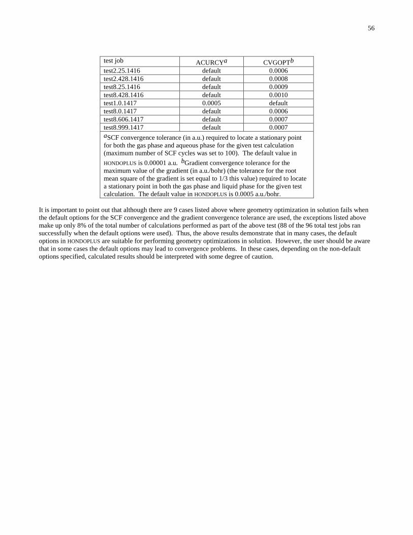
56

test job ACURCYa CVGOPTb

test2.25.1416 default 0.0006

test2.428.1416 default 0.0008

test8.25.1416 default 0.0009

test8.428.1416 default 0.0010

test1.0.1417 0.0005 default

test8.0.1417 default 0.0006

test8.606.1417 default 0.0007

test8.999.1417 default 0.0007

aSCF convergence tolerance (in a.u.) required to locate a stationary point

for both the gas phase and aqueous phase for the given test calculation

(maximum number of SCF cycles was set to 100). The default value in

HONDOPLUS is 0.00001 a.u. bGradient convergence tolerance for the

maximum value of the gradient (in a.u./bohr) (the tolerance for the root

mean square of the gradient is set equal to 1/3 this value) required to locate

a stationary point in both the gas phase and liquid phase for the given test

calculation. The default value in HONDOPLUS is 0.0005 a.u./bohr.

It is important to point out that although there are 9 cases listed above where geometry optimization in solution fails when

the default options for the SCF convergence and the gradient convergence tolerance are used, the exceptions listed above

make up only 8% of the total number of calculations performed as part of the above test (88 of the 96 total test jobs ran

successfully when the default options were used). Thus, the above results demonstrate that in many cases, the default

options in HONDOPLUS are suitable for performing geometry optimizations in solution. However, the user should be aware

that in some cases the default options may lead to convergence problems. In these cases, depending on the non-default

options specified, calculated results should be interpreted with some degree of caution.

57

SCF Schemes for Diffuse Basis Functions

Another important issue that is tested in this section is the difference between using SCF Scheme I and SCF Scheme II for

liquid-phase calculations involving diffuse basis functions. This is an important issue, because past experience has shown

that in some cases, when SCF Scheme I is used with diffuse basis functions, the liquid-phase SCF calculation is unable to

reach convergence (in particular, drastic fluctuations in the Mayer bond orders occur between the gas phase and the liquid

phase when using SCF Scheme I, leading to poor SCF convergence). In cases where this occurs, using SCF Scheme II

usually resolves this problem. (In contrast, this issue rarely arises when non-diffuse basis sets are used, as demonstrated by

the results from above). To test the difference between the results obtained using SCF Scheme I and SCF Scheme II for

basis sets containing diffuse basis functions, we carried out single-point calculations using both SCF Scheme I and SCF

Scheme II, for all jobs with the suffix 1418 (SM6/MPWX/6-31+G* calculations) and 1419 (SM6/MPWX/6-31+G*

calculations). For these calculations, we used gas-phase geometries calculated at the MPW25/MIDI! level of theory as

input. For the test jobs described above, the computed solvation free energy is the difference between the free energy in the

gas phase, evaluated at the MPWX/6-31+G**//MPW25/MIDI! level of theory, and the free energy in the aqueous phase,

evaluated at the SM6/MPWX/6-31+G**//MPW25/MIDI! level of theory. The results of this test are summarized below.

For test jobs test3.a.1b, test4.a.1b, and test5.a.1b, (where a = 0, 25, 428, 517, 606, and 999 and b = 418 and 419) using SCF

Scheme I and SCF Scheme II both led to converged, liquid-phase wave functions when the default value of 10-5 a.u was

used for the SCF convergence tolerance. The computed solvation free energies for these test jobs are listed in the table on

the following page.

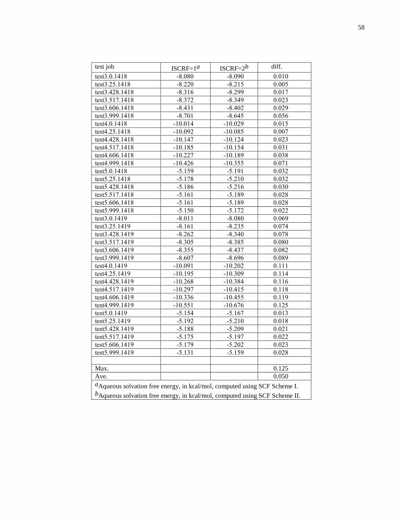
58

test job ISCRF=1a ISCRF=2b diff.

test3.0.1418 -8.080 -8.090 0.010 test3.25.1418 -8.220 -8.215 0.005 test3.428.1418 -8.316 -8.299 0.017 test3.517.1418 -8.372 -8.349 0.023 test3.606.1418 -8.431 -8.402 0.029 test3.999.1418 -8.701 -8.645 0.056 test4.0.1418 -10.014 -10.029 0.015 test4.25.1418 -10.092 -10.085 0.007 test4.428.1418 -10.147 -10.124 0.023 test4.517.1418 -10.185 -10.154 0.031 test4.606.1418 -10.227 -10.189 0.038 test4.999.1418 -10.426 -10.355 0.071 test5.0.1418 -5.159 -5.191 0.032 test5.25.1418 -5.178 -5.210 0.032 test5.428.1418 -5.186 -5.216 0.030 test5.517.1418 -5.161 -5.189 0.028 test5.606.1418 -5.161 -5.189 0.028 test5.999.1418 -5.150 -5.172 0.022 test3.0.1419 -8.011 -8.080 0.069 test3.25.1419 -8.161 -8.235 0.074 test3.428.1419 -8.262 -8.340 0.078 test3.517.1419 -8.305 -8.385 0.080 test3.606.1419 -8.355 -8.437 0.082 test3.999.1419 -8.607 -8.696 0.089 test4.0.1419 -10.091 -10.202 0.111 test4.25.1419 -10.195 -10.309 0.114 test4.428.1419 -10.268 -10.384 0.116 test4.517.1419 -10.297 -10.415 0.118 test4.606.1419 -10.336 -10.455 0.119 test4.999.1419 -10.551 -10.676 0.125 test5.0.1419 -5.154 -5.167 0.013 test5.25.1419 -5.192 -5.210 0.018 test5.428.1419 -5.188 -5.209 0.021 test5.517.1419 -5.175 -5.197 0.022 test5.606.1419 -5.179 -5.202 0.023 test5.999.1419 -5.131 -5.159 0.028

Max. 0.125

Ave. 0.050

aAqueous solvation free energy, in kcal/mol, computed using SCF Scheme I.

bAqueous solvation free energy, in kcal/mol, computed using SCF Scheme II.

59

The table on the preceding page shows that for all test jobs where using SCF Scheme I and SCF Scheme II lead to

converged, liquid-phase wave functions, the differences between the aqueous solvation free energies computed using SCF

Scheme I and those computed using SCF Scheme II are very small in all cases. Even the maximum value of the

difference, 0.125 kcal, is significantly smaller than the average error associated with any of our methods (~ 0.5 kcal in

solvation free energies for neutral solutes).

For the remaining test jobs not shown in the table above (test1.a.1b, test2.a.1b, test6.a.1b, test7.a.1b, and test8.a.1b, where

a = 0, 25, 428, 517, 606, and 999 and b = 418 and 419), using SCF Scheme I led to poor convergence in the SCF

calculation. In all cases, when SCF Scheme II was used instead of SCF Scheme I, the liquid-phase wave functions

converged quite readily (when the default value of 10-5 a.u was used for the SCF convergence tolerance).

Because of the small difference between the aqueous solvation free energies computed using SCF Scheme I and those

computed SCF Scheme II (see table above), and because for the majority of the test cases where diffuse basis functions

were used, SCF Scheme I led to poor convergence, SCF Scheme I is no longer available for calculations that use diffuse

basis-functions.

The input and output files for all of the calculations described above are located in the /sm6 directory. A listing of the input

and output jobs in this directory is given in the table below.

Calculation type test cases

Gas-phase and aqueous-phase (SCF Scheme I) geometry

optimization using SM6/MPWX/MIDI!6D and

SM6/MPWX/6-31G*

testx.a.1416, where w = 1 – 8, and a = 0, 25, 428, 417,

606, and 999.

testx.a.1417, where w = 1 – 8, and a = 0, 25, 428, 417,

606, and 999.

Single-point, aqueous-phase calculation (SCF Scheme I)

using SM6/MPWX/6-31+G* and SM6/MPWX/6-

31+G**

testx.a.1418_1, where w = 1 – 8, and a = 0, 25, 428, 417,

606, and 999.


606, and 999.

Single-point, aqueous-phase calculation (SCF Scheme

II) using SM6/MPWX/6-31+G* and SM6/MPWX/6-

31+G**


606, and 999.


606, and 999.

60

Special notes on basis sets

MIDI! basis set

The MIDI! basis set is defined for H, Li, C, N, O, F, Si, P, S, Cl, Br, and I. The MIDI! basis is similar to the 3-21G basis

set with the following key differences:

The MIDI s and p orbitals have different exponents, whereas the 3-21G valence s orbitals are constrained to have the same

exponents as the p orbitals. (Si, Br, and I, use the 3-21G basis set to which polarization functions were added.)

The bang (!) indicates that there is a d shell on N, O, Si, P, S, Cl, Br, and I and a p shell on Li. There are no p-polarization

functions on hydrogen either. Thus bang is part-way between star and no-star. In the MIDI! basis set, these d shells

(and the p shell for Li) have been carefully optimized to reproduce high quality geometries and partial atomic charges.

Please note the following convention regarding MIDI! basis sets: the original MIDI! basis set used 5 spherical harmonic

components for each d shell; and MIDI! by itself denotes using 5-component d shells. However, we sometimes use 6

Cartesian components for d shells; this is denoted MIDI!6D. For emphasis, sometimes we use MIDI!5D to denote MIDI!.

The MIDI! basis set is stored internally in HONDOPLUS. It may be requested with the MIDIX or MIDI! keyword in the

$BAS or $BASIS data group. In addition, the MIDI! basis set for all available elements is provided in HONDO/HONDOPLUS

format in the file named “midi-bang.bas”, is located in the hondoplus-v5.2/HondoS directory.

6-31G* and 6-31+G* basis sets in CM2, CM3, CM4, and SMx (x = 5.42, 5.43, 6 and 6T)

Whenever we refer to the 6-31G* and 6-31+G* basis sets in conjunction with CM2, CM3, and/or SMx (x = 5.42, 5.43, 6

and 6T), we refer to these basis sets as extended in “A New Class IV Charge Model for Extracting Accurate Partial Charges

from Wave Functions,” Li, J.; Zhu, T.; Cramer, C. J.; Truhlar, D. G. J. Phys. Chem. A 1998, 102, 1820-1831. The 6-31G*

basis set was not available for I, so we used the MIDI!6D instead. In addition, the 6-31+G* basis set was also not available

for I, so we used the MIDI!6D basis set augmented by diffuse s and p shells each having an exponent 0.03. The extended

6-31G* and 6-31+G* basis sets in HONDO/HONDOPLUS format are provided in the files named “6-31GS.bas” and

“6-31PGS.bas,” respectively. These files are located in the hondoplus-v5.2/HondoS directory. The 6-31G* basis set is

stored internally in HONDOPLUS, while the 6-31+G* basis set is not. Thus the 6-31+G* must always be inputted as a

general basis set, and 6-31G* must be inputted as a general basis set for molecules containing iodine.

For Si, a 6-31G and 6-31G* basis has been developed independently by Gordon (Gordon, M.S. Chem. Phys. Lett. 1980, 76,

163), and by Francl et al. (Francl, M. M.; Petro, W. J.; Hehre, W. J.; Binkley, J. S.; Gordon, M. S.; DeFrees, D. J.; Pople, J.

A. J. Chem. Phys. 1982, 77, 3654). The two basis sets give quantitatively different results. For example, silane optimized

using Gordon’s 6-31G* basis set gives an energy of -291.2246 hartrees and a Si-H bond length of 1.481 angstroms,

whereas Francl et al 6-31G* basis set yields an energy of -291.2251 hartrees and a Si-H bond length of 1.476 angstroms.

Both basis sets have been implemented in HONDOPLUS; the former can be requested with the 6-31GA, 6-31GA*, or

6-31GA** keyword in the $BAS or $BASIS data group and the latter can be requested with the 6-31G, 6-31G*, or

6-31G** keyword. The CM2 and SM5.42 parameterizations for Si used the 6-31G* basis set developed by Francl and

co-workers. This version of the basis set should be used if a CM2 or SM5.42 calculation with the 6-31G* basis set is

performed for a molecule containing Si. However, we have observed very small differences in results for several Si

containing compounds when either basis is used (see Winget, P.; Thompson, J. D.; Cramer, C. J.; Truhlar, D. G., J. Phys.

Chem. B, 2001, 106, 5160).

Version 3.4 of HONDOPLUS is the first version that has the 6-31G and 6-31G* basis sets for third row atoms stored

internally. For K and Ca, there are two versions of 6-31G* that have been implemented (they differ only in the value of the

exponents of the polarization functions). Both versions use the 6-31G basis set that is implemented in GAUSSIAN (see

“6-31G* basis set for atoms K through Zn” Rassolov, V. A.; Pople, J. A.; Ratner, M. A.; Windus, T. L., J. Chem. Phys.

1998, 109, 1223). The polarization functions used in the GAUSSIAN version of 6-31G* for K and Ca come from “Extension

61

of Gaussian-2 (G2) theory to molecules containing third-row atoms K and Ca” Blaudeau, J.; McGrath, M. P.; Curtiss, L.

A.; Radom, L. J. Chem. Phys. 1997, 13, 5016. However, a second version of the polarization functions have also been

developed (see “6-31G* Basis Set for Third-Row Atoms” Rassolov, V. A.; Ratner, M. A.; Pople, J. A.; Redfern, P. C.;

Curtiss, L. A. J. Comput. Chem. 2001, 22, 976). The GAUSSIAN version of 6-31G* for K and Ca may be requested with the

6-31G, 6-31G*, and 6-31G** keywords in the $BAS or $BASIS data group, and the other version may be requested with

the 6-31GA (which would be identical to using the 6-31G keyword), 6-31GA*, and 6-31GA** keywords.

For third row transition metals, only one version of 6-31G and 6-31G* exists (see “6-31G* basis set for atoms K through

Zn” Rassolov, V. A.; Pople, J. A.; Ratner, M. A.; Windus, T. L. J. Chem. Phys. 1998, 109, 1223). The authors of this work

note that more stable results are obtained when spherical harmonic f polarization functions are used. We therefore suggest

spherical harmonic f functions be used, i.e., by setting ISPHER equal to 1 in the $CNTRL or $CTL namelist when 6-31G*

is used. Note that the test case for scandium using spherical harmonic f polarization functions gives a slightly different

electronic energy than that given in the paper mentioned above. This is because the authors used Cartesian d functions with

spherical harmonic f functions. However, when ISPHER is set equal to 1, both spherical harmonic d and f functions are

used in the calculation. Note also that identical results will be obtained when either 6-31G or 6-31GA, 6-31G* or

6-31GA*, or 6-31G** or 6-31GA** is used and when a third row transition metal is present in the molecule and Si is not.

For Ga – Kr, HONDOPLUS implements the 6-31G and 6-31G* basis set implemented in GAUSSIAN (see “Compact Contracted

Basis Sets for Third-Row Atoms: Ga – Kr” Binning, R. C., Jr.; Curtiss, L. A. J. Comp. Chem. 1990, 11, 1206). It can be

requested with the 6-31G, 6-31G*, and 6-31G** keywords. HONDOPLUS also implements the 6-31G and 6-31G* basis sets

proposed in “6-31G* Basis Set for Third-Row Atoms” Rassolov, V. A.; Ratner, M. A.; Pople, J. A.; Redfern, P. C.; Curtiss,

L. A. J. Comp. Chem. 2001, 22, 976. It can be requested with the 6-31GA, 6-31GA*, or 6-31GA** keywords. When the

CM2 or SM5.42 model calculation is requested for a system containing Br, the user should use the 6-31G* keyword, not

the 6-31GA* keyword because the GAUSSIAN versions were used in the parameterizations.

cc-pVDZ basis set

Whenever we refer to the cc-pVDZ basis sets in conjunction with CM2 and/or SM5.42R, we refer to the cc-pVDZ basis set

as extended in “Accurate Dipole Moments from Hartree-Fock Calculations by Means of Class IV Charges,” Li, J.; Xing, J.;

Cramer, C. J.; Truhlar, D. G. J. Chem. Phys. 1999, 111, 885-892. This extended basis set is identical to the cc-pVDZ basis

set for all elements except Br and I; for Br and I we use the MIDI! basis set. This extended cc-pVDZ basis set must be

inputted as a general basis set. The cc-pVDZ basis sets for all available elements are provided in HONDO format in the file

named “ccpVDZ.bas” is located in the HondoS/Input directory.

MG3 and MG3S basis set

The MG3 and MG3S basis sets were defined to use spherical harmonic d and f functions. Therefore, when using one of

these basis sets, ISPHER should be defined to be equal to 1 in $CNTRL or $CTL.

SCF schemes

If ISCRF = 0, only a gas-phase calculation is done, and this is the default. If ISCRF equals either 1 or 2, then the code

does a liquid-phase SCF calculation. Two different SCF schemes have been implemented. The standard scheme, called

scheme I, uses the current solution-phase bond order matrix values in in the Fock or Kohn-Sham operator at every step of

the iteration. Scheme I is chosen by setting ISCRF = 1.

Scheme II uses the gas-phase bond order matrix values at the current geometry to calculate CM2, CM3, or CM4 corrections

of Löwdin or RLPA charges in solution. Scheme II and its physical meaning may be “justified” as follows. The

modification to the Löwdin or RLPA charges is parameterized to fit to experimental gas-phase dipole moments. So one can

assume that the same modification applies to the solvated molecule with the same geometry in the liquid phase as in the gas

62

phase. The change of atomic partial charges due to the solvation effects is reflected by the change of Löwdin or RLPA

charges, and all qkM

are constants. This leads to a very simple expression for solvated Fock matrix elements:

FijS Fij

g Vkn (S

1

2

n )in(S

1

2 )nj (15)

whereVkn is the reaction field acting on atom k according to Eq. (3), i, j, and n are basis functions, and kn is the atom on

which basis function n is centered.

Usually scheme I and scheme II give very similar results. In principle (and in practice), scheme II converges to slightly

different results, and thus it could be considered to be a different model. However, in our experience the difference is

usually small, and scheme II sometimes has better convergence properties.

SCF Scheme III (ISCRF = 3) performs a liquid-phase SCRF based on user-provided atomic charges

(ICREAD = 1). These atomic charges remain constant during the SCRF calculation. Analytical gradients have not been

implemented for ISCRF = 3.

63

Density Functional Methods Recommended for use with CM4 and SM6 in HONDOPLUS

The CM4 and SM6 model can be used with any density functional, as long as the density functional gives a reasonable

electronic distribution for the molecule of interest. Shown in the table below is a list of density functional methods

recommended for use with CM4 and SM6 that are available in HONDOPLUS. For the hybrid density functional theory

methods supported in HONDOPLUS, the percent Hartree-Fock exchange for each functional is also given.

Pure DFT functionals recommended for use with CM4 and SM6 in HONDOPLUS. Note that the keyword HFE=0.00 should be

specified when these, or any other pure DFT functionals are used in conjunction with the CM4 or SM6 models .

Method HONDOPLUS Keyword Reference(s)

BLYP DFTFUN=5 A. D. Becke, Phys. Rev. A 38, 3098 (1988).

C. Lee, W. Yang, and R. G. Parr, Phys. Rev. B 37, 785 (1988).

B. Miehlich, A. Savin, H. Stoll, and H. Preuss, Chem. Phys. Lett. 157, 200

(1989).

BPW91 DFTFUN=7 A. D. Becke, Phys. Rev. A 38, 3098 (1988).

K. Burke, J. P. Perdew, and Y. Wang, in Electronic Density Functional

Theory: Recent Progress and New Directions, Ed. J. F. Dobson, G.

Vignale, and M. P. Das (Plenum, 1998).

J. P. Perdew, in Electronic Structure of Solids ‘ 91, Ed. P. Ziesche and H.

Eschrig (Akademie Verlag, Berlin, 1991) 11.

J. P. Perdew, J. A. Chevary, S. H. Vosko, K. A. Jackson, M. R. Pederson,

D. J. Singh, and C. Fiolhais, Phys. Rev. B 46, (1992).



J. P. Perdew, K. Burke, and Y. Wang, Phys. Rev. B 54, 16533 (1996).

mPWPW91

(also called

mPWPW)

DFTFUN=3000 C. Adamo and V. Barone, J. Chem. Phys. 108, 664 (1998).

K. Burke, J. P. Perdew, and Y. Wang, in Electronic Density Functional

Theory: Recent Progress and New Directions, Ed. J. F. Dobson, G.

Vignale, and M. P. Das (Plenum, 1998)

J. P. Perdew, in Electronic Structure of Solids ‘ 91, Ed. P. Ziesche and H.

Eschrig (Akademie Verlag, Berlin, 1991) 11





J. P. Perdew, K. Burke, and Y. Wang, Phys. Rev. B 54, 16533 (1996).

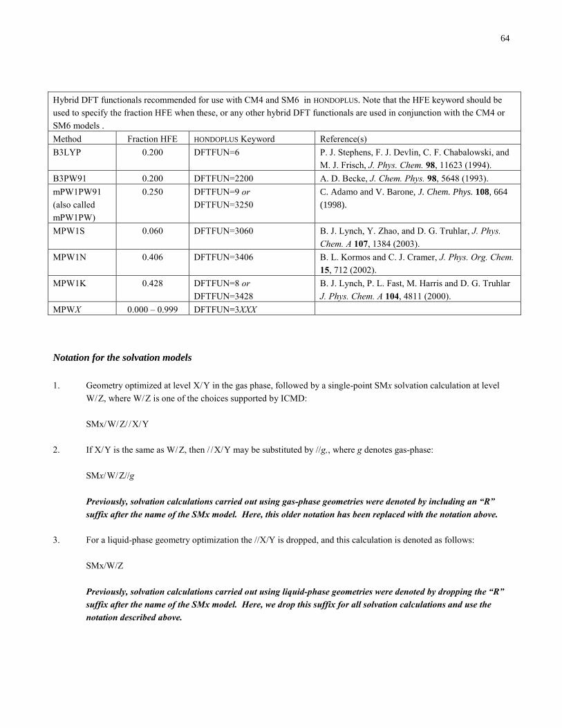
64

Hybrid DFT functionals recommended for use with CM4 and SM6 in HONDOPLUS. Note that the HFE keyword should be

used to specify the fraction HFE when these, or any other hybrid DFT functionals are used in conjunction with the CM4 or

SM6 models .

Method Fraction HFE HONDOPLUS Keyword Reference(s)

B3LYP 0.200 DFTFUN=6 P. J. Stephens, F. J. Devlin, C. F. Chabalowski, and

M. J. Frisch, J. Phys. Chem. 98, 11623 (1994).

B3PW91 0.200 DFTFUN=2200 A. D. Becke, J. Chem. Phys. 98, 5648 (1993).

mPW1PW91

(also called

mPW1PW)

0.250 DFTFUN=9 or

DFTFUN=3250

C. Adamo and V. Barone, J. Chem. Phys. 108, 664

(1998).

MPW1S 0.060 DFTFUN=3060 B. J. Lynch, Y. Zhao, and D. G. Truhlar, J. Phys.

Chem. A 107, 1384 (2003).

MPW1N 0.406 DFTFUN=3406 B. L. Kormos and C. J. Cramer, J. Phys. Org. Chem.

15, 712 (2002).

MPW1K 0.428 DFTFUN=8 or

DFTFUN=3428

B. J. Lynch, P. L. Fast, M. Harris and D. G. Truhlar

J. Phys. Chem. A 104, 4811 (2000).

MPWX 0.000 – 0.999 DFTFUN=3XXX

Notation for the solvation models

1. Geometry optimized at level X/Y in the gas phase, followed by a single-point SMx solvation calculation at level

W/Z, where W/Z is one of the choices supported by ICMD:

SMx/W/Z/ /X/Y

2. If X/Y is the same as W/Z, then / /X/Y may be substituted by //g,, where g denotes gas-phase:

SMx/W/Z//g

Previously, solvation calculations carried out using gas-phase geometries were denoted by including an “R”

suffix after the name of the SMx model. Here, this older notation has been replaced with the notation above.

3. For a liquid-phase geometry optimization the //X/Y is dropped, and this calculation is denoted as follows:

SMx/W/Z

Previously, solvation calculations carried out using liquid-phase geometries were denoted by dropping the “R”

suffix after the name of the SMx model. Here, we drop this suffix for all solvation calculations and use the

notation described above.

65

Executive summary for the diabatization method

The algorithm for diabatization is based on the configurational uniformity concept. Diabatic configuration state functions

(DCSFs) are constructed in terms of diabatic molecular orbitals (DMOs) that are determined by the fourfold way. Presently

the program assumes that adiabatic states are CASSCF or CASSCF+MCQDPT wave functions. The inactive and external

orbitals are the canonical orbitals of the CASSCF calculation, and the fourfold way is applied only to the active orbitals.

Theoretical background for diabatization

Quasidiabatic states

N diabatic states k (k=1…..N) can be represented by a unitary transformation of N adiabatic states k, where N is the total

number of electronic states includes in the dynamics; and usually N is the number of electronic states whose adiabatic

energies are so close that one cannot neglect nonadiabatic vector couplings. Electronic states with vanishing nonadiabatic

vector couplings are called strict diabatic states; however such strict diabatic states do not exist in the general case.

Quasidiabatic states are defined as states for which scalar couplings (i.e., off-diagonal elements of the electronic

Hamiltonian, and called diabatic couplings) are much larger than their vector couplings. Usually quasidiabatic states are

called diabatic states, and this terminology is used in this manual.

There are many methods to calculate diabatic states, and the one available in HONDOPLUS is based on an orthogonal

transformation of variationally determined adiabatic states. Such a transformation may be based on matrix elements of the

nuclear-momentum operator, which yields a “dynamical” approach or on some measurement of smoothness of the wave

functions against changes of nuclear geometry. The method in HONDOPLUS is based on such a smoothness criterion,

introduced in:

H. Nakamura and D. G. Truhlar, “The direct calculation of diabatic states based on configurational uniformity,” J.

Chem. Phys. 115 10353 (2001).

Configurational uniformity

The configurational uniformity scheme is a method for defining diabatic states that is based on smoothness, and it has

several desirable properties for calculating global, physically reasonable diabatic potential energy surfaces (PESs) , in

particular:

1. The resulting diabatic states are unique (within a scheme) for each nuclear geometry.

2. Diabatization is carried out by using only adiabatic wave functions and electronic Hamiltonian matrix

elements with no other matrix elements required.

3. The procedure is systematic and the same for any molecular system.

To apply the configurational uniformity scheme, dominant CSF groups Gk (k = 1….N) must be defined. The basis CSFs in

a group Gk are prototypes for diabatic state k. Each of the basis CSFs in each group must belong to the same group over

the entire nuclear coordinate space. A geometry in regions where adiabatic states are, to good approximation, the same as

diabatic states is called a “potential reference geometry”. Therefore are many potential reference geometries.

Practically one can use one or more of the potential reference geometries, e.g. an equilibrium geometry or geometries in

asymptotic regions of a reaction to construct dominant CSF lists by calculating adiabatic states at these geometries. A

geometry actually used to make dominant CSF lists is called a “reference geometry”. When one treats a rearrangement

reaction system, one may require physically reasonable diabatic PESs that agree with adiabatic PESs in asymptotic regions

of both (or all, if more than two) arrangements (i.e., potential reference geometries exist in both arrangements, and

sometimes we must use them in more than one arrangement.) In such cases, a single reference geometry is not enough, and

consistent dominant CSF group lists must be constructed by considering dominant CSFs in both (or all) arrangements, i.e.,

two or more reference geometries are required. Note that dominant CSFs in Gk are not necessarily always dominant in all

potential reference geometries simultaneously, but at least one CSF of Gk is dominant for k in any nuclear geometry.

66

The fourfold way

To construct CSFs, appropriate MOs are required. In order for the configurational uniformity approach to give

suitable diabatic states, the follow conditions are required to be met:

The deformation of MOs is smooth/or smooth enough along continuous nuclear coordinate paths. (This is

called “MO uniformity”.)

The MOs should give a small number of dominant CSFs at potential reference geometries.

MOs meeting these requirements are called diabatic MOs (DMOs) and are determined by the fourfold way. To identify

dominant CSFs, inactive orbitals (which are doubly occupied in all configurations) and virtual orbitals need not be

considered; therefore the fourfold way is applied to only active MOs, where the total number of active MOs is called . To

distinguish the MOs used initially to calculate the adiabatic states from the DMOs, we call the former “adiabatic MOs”

(AMOs). The sequence of steps is as follows. First the DMOs are defined by transformation of the AMOs, and the adiabatic

states are re-expanded in term of the DMOs; then the configurational uniformity scheme is performed. Since the CASSCF

wave functions are invariant to orbital rotation in the active space, the space spanned by DMOs may be considered to be

energetically optimized, just like the space spanned by the AMOs.

The fourfold way consists of two criteria: the threefold density criterion and the MORMO criterion. The threefold density

criterion consists in maximizing the D3 function giving by:

D3(N,R,T)=ND(NO)

+RD(ON)

+TD(TD)

where NRand Tare parameters and are usually fixed as 2, 1, and 0.5. D(NO)

is the natural orbital term and is a function

of diagonal elements of the state-averaged density matrix. D(ON)

is the occupation number term and is defined by using

density matrices of each of the adiabatic states. The transition density term D(TD)

is based on the transition density matrix

elements.

The MORMO criterion involves maximizing the MORMO term D(RO)

, which is a sum of the squares of overlaps of MOs

with the reference MOs u(ref)

(Q):

D(RO)

= =1

|<u(ref)

|u>|2

and u(ref)

(Q) is defined as

u(ref)

(Q)=i

ai(Q(ref)

)i(Q)

where i(Q) is an atomic orbital (i.e., basis function) at the current geometry Q, and ai(Q(ref)

) is an MO coefficient of the

DMO at the reference geometry Q(ref)

. In the present algorithm, we assume that reference MOs are defined by the DMOs at

one reference geometry. This one particular reference geometry that is used for this purpose is called the MORMO

reference geometry. Thus if there is more than one reference geometry, one needs to select one reference geometry where

reference MOs are defined. The fourfold way is carried out by the following steps:

By the MORMO criterion, DMOs are determined by orbital rotation within the active space. In this process, any elements

of corresponding density matrices are also transformed. Since the total number of active MOs is is less than or equal to

. Usually is much smaller than . The choice of is discussed further below.

The new D3 function, that is constructed by using density matrix elements corresponding to only non-reference orbitals,

is calculated. (To make the notation clear, this function is referred to as D3free

.)

The threefold density criterion is applied to the D3free

function; in this way the remaining DMOs are determined.

67

The threefold density criterion can always give suitable DMOs in any of the potential reference geometries; thus dominant

CSF group lists can be obtained without reference MOs. How to select reference MOs depends on the dominant CSF lists,

and the strategy will be summarized in the next section.

Usage for diabatization: How to calculate diabatic potentials with HONDOPLUS

The main part of the input for diabatization is in the namelists $DIABAT and $PROTOTYPE and the data groups

$CSFDAT, $DIAVEC, and $DFMVEC. The program performs diabatization after calculation of adiabatic CASSCF or

CASSCF/MCQDPT wave functions; thus inputs for CASSCF or CASSCF/MCQDPT are also necessary.

Although the algorithm for diabatization is systematic and general, this does not mean that the procedure is a black-box

procedure. Especially the preliminary parts, constructing dominant CSF groups and selection of the reference MOs, may

require some trial calculations and analysis of the results, perhaps combined with a knowledge of the relevant physics for

the system under consideration. In this section, some topics relating to practical calculation as well as brief explanations of

parameters are given. More details of the input will be given in a later part of this manual. For the details of a practical

strategy for calculations, see these papers:

H. Nakamura and D. G. Truhlar, ”The direct calculation of diabatic states based on configurational uniformity,” J.

Chem. Phys. 115, 10353 (2001).

H. Nakamura and D. G. Truhlar, “Direct diabatization of electronic states by the fourfold way: II. Dynamical

correlation and rearrangement processes,” J. Chem. Phys. 117 5576 (2002).

H. Nakamura and D. G. Truhlar, “Extension of the fourfold way for calculation of global diabatic potential energy

surfaces of complex, multiarragement, non-Born-Oppenheimer systems: Application to HNCO(S0,S1),” J. Chem.

Phys. 118 6816 (2003).

R. Valero and D. G. Truhlar, “Nonadiabatic effects in C-Br scission in the photodissociation of bromoacetyl

chloride”, J. Chem. Phys. 125 194305 (2006).

K. R. Yang, X. Xu, and D. G. Truhlar, “Direct Diabatization of electronic states by the fourfold way: Including

dynamical correlation by multi-configuration quasidegenerate perturbation theory with complete active space self-

consistent-field diabatic molecular orbitals”, Chem. Phys. Lett., submitted.

Ordering of DMOs

To apply the configurational uniformity scheme, the CSFs must be labeled consistently over the entire nuclear coordinate

space; thus DMOs have to be ordered correctly. Suppose that DMOs are obtained at a nuclear geometry Q', and CSFs are

labeled by this set of DMOs. As the next step, DMOs u(Q) of the current geometry Q may be ordered with one-to-one

correspondence between each u(Q) and the corresponding u(Q'). The one-to-one correspondence is identified, for

example, by estimating an overlap-like quantity (Q,Q') as follows;

)',(|)()',( QQvQuQQ ,

where v(Q ,Q') is used to approximate u(Q'),

v(Q, Q')=i

ai(Q') i(Q)

68

where i(Q) is an atomic basis function, and ai(Q') is the MO coefficient of the DMO at Q'. We call v(Q ,Q') an “order

reference MO”. To get a suitable one-to-one correspondence, Q and Q' should be close enough. Note that this does not

mean that the results are path dependent, because the DMOs at Q are defined by the fourfold way, and the order reference

MOs are used to order the resulting DMOs. In addition, one has to define a consistent molecular orientation to order DMOs

by the above overlap-like quantity.

In the program, the DMOs u(Q) are ordered by the data group $DFMVEC in input. $DFMVEC contains MO coefficients

to make order reference MOs. The procedure is follows;

1. Read $DFMVEC from input.

2. Construct order reference MOs v(Q) that are defined by symmetric orthogonalization of orbitals of

$DFMVEC. (Thus the MO coefficients of the order reference MOs used in the program are slightly different

from the data in $DFMVEC.)

3. Estimate the overlap-like quantity between sets of u and v, and search for one-to-one correspondence.

To use $DFMVEC for ordering, the option NDFRM ($DIABAT) must be set to 1. When NDFRM is set to 0, the order

reference MOs are defined by the canonical orbitals (AMOs) which are obtained in the CASSCF step. (Strictly speaking,

the CASSCF method does not determine individual MOs uniquely; thus the definition of the AMOs is somewhat arbitrary

in the CASSCF method. Therefore we take AMOs to be canonical MOs for the CASSCF wave functions.) The MO

coefficients of the ordered DMOs obtained at the current geometry are written out to the *pun file (FT07) as $DFMVEC.

Therefore one can use this data written as $DFMVEC to make a new input of calculation of another geometry.

Labeling of CSFs and dominant CSF group lists

The candidates for dominant CSFs are obtained by calculations at reference geometries with the threefold density criterion.

The label of each CSF is identified by GUGA (graphical unitary group approach), just as in the CI section of HONDO. If

the option NRCSF ($DIABAT) is set to 0, the program simply picks CSFs that have larger absolute values of CI

coefficients than SLCTTH ($DIABAT) as dominant CSFs; then it assigns dominant CSFs of the adiabatic state k to the

group Gk. If NRCSF=1, the program reads data group $CSFDAT in input and uses dominant CSF group lists defined in

$CSFDAT. $CSFDAT consists of CI coefficients correlating to the CSFs written in $CSFDAT. These CI coefficients are

expansion coefficients of diabatic states obtained by transformation of adiabatic CI wave functions. In both cases, the new

$CSFDAT is written to the *pun file. To get a suitable sign (phase factor) for diabatic states, $CSFDAT may be required

to be updated for new input, just like $DFMVEC.

Since $CSFDAT defines dominant CSF groups, one may need some trial calculations and manual modification of

$CSFDAT obtained by these trial calculations. As an example, when a system has two or more arrangements, one has to

take suitable reference geometries and make lists from these geometries to make $CSFDAT. This preliminary procedure is

necessary. After $CSFDAT is fixed, then it is simply updated to determine consistent phase factors of diabatic states. (By

setting NRCSF=1, the dominant CSF groups are fixed; thus the $CSFDAT written to *pun file contains only the same

CSFs as in the input.) Recall that a one-to-one correspondence between different reference geometries must be established

to label CSFs consistently.

Determination of DMOs

Although the threefold density criterion gives suitable DMOs at each potential reference geometry, the MORMO criterion

is necessary for a general nuclear geometry. To apply the fourfold way, one has to define the reference MOs to apply the

MORMO criterion. The current algorithm assumes that the reference MOs are defined by the DMOs at the MORMO

reference geometry, which is one of the reference geometries, as explained above.

Selection of the reference MOs is based on the fundamental CSF pattern of the dominant CSFs. Assume that the CSF 1 is

in G1, and 2 is in G2. The fundamental CSF patterns are defined as follows;

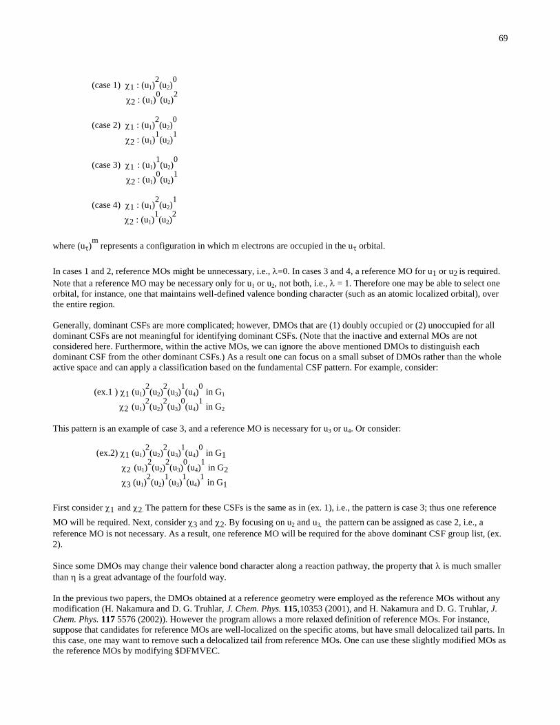
69

(case 1) 1 : (u1)2(u2)

0

2 : (u1)0(u2)

2

(case 2) 1 : (u1)2(u2)

0

2 : (u1)1(u2)

1

(case 3) 1 : (u1)1(u2)

0

2 : (u1)0(u2)

1

(case 4) 1 : (u1)2(u2)

1

2 : (u1)1(u2)

2

where (u)m

represents a configuration in which m electrons are occupied in the u orbital.

In cases 1 and 2, reference MOs might be unnecessary, i.e.,=0. In cases 3 and 4, a reference MO for u1 or u2 is required.

Note that a reference MO may be necessary only for u1 or u2, not both, i.e.,= 1. Therefore one may be able to select one

orbital, for instance, one that maintains well-defined valence bonding character (such as an atomic localized orbital), over

the entire region.

Generally, dominant CSFs are more complicated; however, DMOs that are (1) doubly occupied or (2) unoccupied for all

dominant CSFs are not meaningful for identifying dominant CSFs. (Note that the inactive and external MOs are not

considered here. Furthermore, within the active MOs, we can ignore the above mentioned DMOs to distinguish each

dominant CSF from the other dominant CSFs.) As a result one can focus on a small subset of DMOs rather than the whole

active space and can apply a classification based on the fundamental CSF pattern. For example, consider:

(ex.1 ) 1 (u1)2(u2)

2(u3)

1(u4)

0 in G1

2 (u1)2(u2)

2(u3)

0(u4)

1 in G2

This pattern is an example of case 3, and a reference MO is necessary for u3 or u4. Or consider:

(ex.2) 1 (u1)2(u2)

2(u3)

1(u4)

0 in G1

2 (u1)2(u2)

2(u3)

0(u4)

1 in G2

3 (u1)2(u2)

1(u3)

1(u4)

1 in G1

First consider 1 and 2. The pattern for these CSFs is the same as in (ex. 1), i.e., the pattern is case 3; thus one reference

MO will be required. Next, consider 3 and 2. By focusing on u2 and u3, the pattern can be assigned as case 2, i.e., a

reference MO is not necessary. As a result, one reference MO will be required for the above dominant CSF group list, (ex.

2).

Since some DMOs may change their valence bond character along a reaction pathway, the property that is much smaller

than is a great advantage of the fourfold way.

In the previous two papers, the DMOs obtained at a reference geometry were employed as the reference MOs without any

modification (H. Nakamura and D. G. Truhlar, J. Chem. Phys. 115,10353 (2001), and H. Nakamura and D. G. Truhlar, J.

Chem. Phys. 117 5576 (2002)). However the program allows a more relaxed definition of reference MOs. For instance,

suppose that candidates for reference MOs are well-localized on the specific atoms, but have small delocalized tail parts. In

this case, one may want to remove such a delocalized tail from reference MOs. One can use these slightly modified MOs as

the reference MOs by modifying $DFMVEC.

70

In the program, is equal to the number of active orbitals in both CASSCF and MCQDPT calculations. The total number

of reference MOs is specified by NMLAP ($PROTOTYPE) in input. The MO coefficients of reference MOs are specified

by data group $DIAVEC. Note that $DIAVEC must be fixed for all calculations of diabatic potentials to define a unique

set of surfaces within the procedure.

Symmetry of wave functions and DMOs

The CASSCF and MCQDPT program can calculate specified adiabatic wave functions based on point groups. (See

$CNTRL and $BASIS). The irreps of the target wave functions are identified by $DRT with irreps of MOs.

Although diabatic wave functions belong to the same irreps as the adiabatic wave functions, there is no guarantee that

DMOs have definite symmetry. However, in our experience, symmetry-unconstrained DMOs (i.e., DMOs that are not

enforced to belong to specific irreps) are often almost equal to symmetry-constrained DMOs. If one focuses on diabatic

PESs in only a restricted region, where the molecule keeps the same symmetry, it is useful to employ symmetry-constrained

DMOs because the use of symmetry-constrained MOs reduces drastically the total number of CSFs in the CAS-CI space.

An important example is a triatomic molecule. In this case, Cs symmetry is always conserved, and adiabatic states can be

calculated with a Cs symmetry constraint. As a result DMOs should be constrained to A' or A" irreps.

The program performs the fourfold way with separate orbital rotation for each irrep block when NDMOSYM ($DIABAT)

is set to 0. When NDMOSYM=0, the irrep of each of the reference orbitals specified by $DIAVEC are assigned. (If

$DIAVEC data do not satisfy the symmetry, the program will assign an irrep to which they are closest.) The MORMO

criterion is carried out by orbital rotation within only the subset of MOs that belong to the same irrep of each of the

reference MOs.

If NDMOSYM=1, the fourfold way is performed without any symmetry constraint for MOs. In this case the active space is

invariant, but there is a possibility that states that belong to different irreps than the irreps of the required states are found as

CI roots when these DMOs are used for a CAS-CI calculation. Since diabatization must include only the target adiabatic

states, such states that belong to different irreps must be dropped. In the program, the states that belong to the same irrep

are found automatically. To do so, one needs to set NSTRY ($DIABAT). For instance if NSTRY=4, the CI problem is

solved until it finds the lowest four roots without symmetry constraint. Then the required states that belong to the same

irrep are found from these four roots. If all the required states are not found in the eigenvectors associated with these four

roots, the program will stop with an error message. The user must then set a larger value for NSTRY. Note that CASSCF or

MCQDPT calculations themselves are performed with symmetry constraints (i.e. the AMOs belong to specific irreps)

specified by $BASIS, $DRT and $MCQDPT. If the molecule has no symmetry, NDMOSYM=1 is not meaningful.

Usually NDMOSYM=1 is used at only a few geometries (e.g., reference geometries) to check if the symmetry-constrained

DMOs are really similar to symmetry-unconstrained DMOs. Again, this is true in almost all cases.

Restriction of orbital rotation based on dominant CSFs

As an extension of the original fourfold way, one can separate the active space (i.e., the space where an orbital rotation is

performed) into blocks. The blocks are, in particular, the three blocks: doubly occupied (DC), valence (VL), and virtual

(VIR) blocks. The blocks are specified by the array MOSLAB_CHARACT ($DIABAT) as follows;.

MOSLAB_CHARACT(I)=2 …… I th DMO belongs to DC block

MOSLAB_CHARACT(I)=1 …… I th DMO belongs to VL block

MOSLAB_CHARACT(I)=0 …… I th DMO belongs to VIR block

The DC block must contain only DMOs that are doubly occupied for any dominant CSFs in any group. The MOs assigned

to the VIR block should be unoccupied orbitals in all of the dominant CSFs. The remaining MOs are placed in the VL

block, and the MOs of the VL block contribute to identifying each dominant CSF, because only DMOs in the VL block

have different electronic occupation numbers in each dominant CSF. In other words, determination of DMOs in the VL

71

block is most critical. The whole active space can be treated as the VL block (i.e., one need not use the separation into three

blocks) if the separation is not necessary, and this is the default (in which case the fourfold way is carried out by rotation of

all active orbitals). Suppose, however, that we can separate the active space into these three blocks; in this case, we may be

able to perform the orbital rotation in the fourfold way within only the VL block.

This separation into these blocks and the restriction of orbital rotation can be justified by the following consideration.

Suppose that we have suitable dominant CSF lists and can define the three blocks. From the definition of the DC block, the

MOs in the DC block do not give a contribution to distinguish a dominant CSF from the other dominant CSFs. Thus the

MOs of the DC block can be removed from the target of the fourfold way. For the VIR block, one can make a similar

consideration. The MOs in the VIR block give no contribution to distinguish a dominant CSF from the other dominant

CSFs; therefore these MOs also can be removed from the target of the fourfold way. As a result, as far as one can extract

such MOs that are always doubly occupied MOs (DC) or unoccupied MOs (VIR) for all dominant CSFs, these MOs may

not be required to be included in the fourfold way process. In other words, we can employ MOs in the DC and the VL

blocks as the DMOs without modification. However, the AMOs are not always suitable as MOs in the DC or VIR block. In

other words, some preliminary procedure will be required to separate orbitals into the three blocks before applying the

fourfold way.

In the program, the temporary DMOs are determined by the threefold density criterion as the first preliminary procedure. If

L MOs are specified as being in the DC block by the given dominant CSF list, the program takes temporary DMOs whose

averaged occupation numbers are larger than the threshold TH_DOC ($DIABAT) as candidate MOs of the DC block.

Then L DMOs are determined as the members of the DC block from these candidates by estimating overlap-like quantity

with $DFMVEC. By a similar procedure, where candidates are taken as the temporary DMOs that have smaller averaged

occupation number than TH_VIR ($DIABAT), the VIR block is determined. The DMOs of the DC and the VIR block are

determined in this processes, i.e. they are equal to the temporary DMOs, themselves. As the last step, the fourfold way is

applied to the remaining temporary DMOs which are assigned to MOs in VL block. Thus the temporary DMOs and the

resulting DMOs are different in VL block part. Recall that input that has no DOC or no VIR block is allowed, and this is

recommended in usual cases. The use of MOSLAB_CHARACT may be useful for diabatization for rearrangement

processes of complex molecules. We note that this procedure uses $DFMVEC, however it is used to select the MOs in the

DC and VIR blocks from temporary (candidate) DMOs, and each temporary DMOs are independently of $DFMVEC as

well as DMOs in the VL block. Therefore the resulting DMOs are independent of a path through a nuclear coordinate space.

As a example to indicate usefulness of this algorithm, the two lowest singlet states of HNCO may be taken. When the

geometry of HNCO is planar (i.e., Cs symmetry), the two states correlate to A' and A". Thus adiabatic states should agree

with diabatic states in any Cs geometry. In other words any Cs geometry is a potential reference geometry. To describe a

global region, the three dominant CSFs 1, 2, and 3 will be taken as members of group G1. Also the group G2 has 4 as a

dominant CSF. When 12 electrons are distributed in 10 active orbitals, the dominant CSFs are follows:

1: 2222220000

2: 2222121000

: 2222202000

4: 2222211000

By analysis of preliminary calculations, it was determined that one requires a single reference MO, which is the MO that

correlates with the 6th DMO at the reference geometry. The best reference MO is a localized pz orbital on the N atom to

describe all Cs geometries in both H+NCO and HN+CO asymptotic regions (H. Nakamura and D.G. Truhlar, “Extension

of the fourfold way for calculation of global diabatic potential energy surfaces of complex, multiarragement, non-Born-

Oppenheimer systems: Application to HNCO(S0,S1),” J. Chem. Phys. 118 6816 (2003) ). Since any Cs geometry is a

potential reference geometry for this system, the DMOs obtained by the fourfold way should be almost the same as MOs

obtained by the threefold density criterion. To compare these, three types of calculations, (I) the threefold density criterion,

(II) the fourfold way without separation into blocks, and (III) the fourfold way with separation such as

MOSLAB_CHARACT=2,2,2,2,1,1,1,0,0,0, with the same geometry (HNCO molecule region) were performed. Note that

the first four MOs are doubly occupied for all dominant CSFs 1-4, and the last three MOs are virtual for all dominant

CSFs; thus the above separation into the three blocks is allowed. The summary of the results are follows:

72

(I) Threefold density criterion

---- DMOs based on CASSCF (active) ----

VEC = 6 SYM = A EIG/OCC = 1.47144

------------------------------------------

11 2 N Z -.49428 14 2 N Z -.37085 41 4 O Z .38645 44 4

O Z .28292

VEC = 9 SYM = A EIG/OCC = .08990

------------------------------------------

11 2 N Z -.49439 14 2 N Z -.19185 26 3 C Z .62492 29 3

C Z .37888 41 4 O Z -.44933

44 4 O Z -.19121

-----------------------------------------------

CI coefficients of dominant CSFs for all groups

-----------------------------------------------

Adiabatic State # 1 ENERGY = -167.869594033

------------------ -------------

<CSF> <Group #> <Coefficient>

2222220000 1 -.936686

2222121000 1 -.105651

2222202000 1 .005453

2222110000 2 .000000


------------------ -------------


2222220000 1 .000000

2222121000 1 .000000

2222202000 1 .000000

2222110000 2 .932367

(II) Fourfold way without separation into DC, VL, and VIR blocks


VEC = 6 SYM = A EIG/OCC = 1.39141

------------------------------------------

11 2 N Z -.67679 14 2 N Z -.43012


------------------------------------------

11 2 N Z -.26562 26 3 C Z .66720 29 3 C Z .40207 41 4

O Z -.49180 44 4 O Z -.23883

-----------------------------------------------

CI coefficients of dominant CSFs for all groups

-----------------------------------------------


------------------ -------------


2222220000 1 .773015

73

2222121000 1 .110070

2222202000 1 -.008040

2222211000 2 .000000

2222210010 U -.533913


------------------ -------------


2222220000 1 .000000

2222121000 1 .000000

2222202000 1 .000000

2222211000 2 .822497

2212221000 U .355098

------------------------------------------

The two CSFs 2222210010 and 2212221000 cannot be obtained by the threefold density criterion, i.e., these CSFs cannot

be defined as dominant CSFs, although these CSFs have CI coefficients that are too large to be neglected. (Thus, in the

above we state the group # as U (unknown).

(III) Fourfold way with MOSLAB_CHARACT=2,2,2,2,1,1,1,0,0,0


VEC = 6 SYM = A EIG/OCC = 1.47144

------------------------------------------

11 2 N Z -.49428 14 2 N Z -.37085 41 4 O Z .38645 44 4

O Z .28292


------------------------------------------

11 2 N Z -.49439 14 2 N Z -.19185 26 3 C Z .62492 29 3

C Z .37888 41 4 O Z -.44933

44 4 O Z -.19121

-----------------------------------------------

CI coefficients of dominant CSFs for all Groups

-----------------------------------------------


------------------ -------------


2222220000 1 .936686

2222121000 1 .105651

2222202000 1 -.005453

2222211000 2 .000000


------------------ -------------


2222220000 1 .000000

2222121000 1 .000000

2222202000 1 .000000

2222211000 2 -.932367

------------------------------------------

74

From these results in the cases (I) and (III), the 6th DMO is a orbital bonding N to O, and the 9th DMO is a very

delocalized orbital such as a * orbital in the N-C and C-O bonding regions at this molecular geometry. However in case

(II) the 6th DMO is quite localized on the N atom as a pz orbital (by the MORMO criterion), and the 9th DMO is a *

orbital bonding C to O. Thus the fourfold way without separation into the DC, VL, and VIR blocks provides very different

DMOs from the DMOs obtained by the threefold density criterion although this geometry is potential reference geometry.

CSFs (except 1-4) that are defined as dominant CSFs have large CI coefficients in adiabatic and diabatic wave functions.

Therefore the result of (II) is inconsistent with dominant CSF lists that are defined by the threefold density criterion. As a

result, for instance, the suitable 6th DMO should change its chemical character from a orbital bonding N and O to an

atomic localized orbital on N with change of the arrangements from HN+CO to HNCO and H+NCO although the reference

MO has the chemical character of an atomic localized orbital on N, and case (III) (i.e., the fourfold way with separation into

blocks) can give such suitable DMOs. In other words, use of MOSLAB_CHARACT allows the smooth deformation not

only of DMOs obtained by the D3(free)

functional but also of DMOs fixed by the MORMO criterion in the fourfold way step,

along reaction pathways. This will provide particularly useful flexibility for diabatization in multi-arrangement systems.

Recall that identification of the blocks by MOSLAB_CHARACT depends on the electronic configurations of dominant

CSFs to be used for diabatization, and MOSLAB_CHARACT must be same over the entire nuclear coordinate space.

Input and output files for these calculation are located in the directory master/samples as sample files, sampleS4 (I),

sampleS5 (II) and sampleS6 (III).

Resolution DMOs and specific orientations for reference and resolution DMOs

Further extensions of the fourfold way were implemented for the treatment of complex, multi-arrangement reactions.

Starting with the separation into DC, VL, and VIR blocks, resolution MOs are introduced to determine some (or all) of the

DMOs in the DC block. The main motivation to introduce resolution MOs is to avoid undesirable mixing between DMOs

that belong to different blocks caused by multiple reference geometries. Recall the list of dominant CSFs for HNCO:

1: 2222220000

2: 2222121000

: 2222202000

4: 2222211000

The separation into blocks is carried out according to MOSLAB_CHARACT=2,2,2,2,1,1,1,0,0,0. The 1st, 2

nd, and 4

th

orbitals belonging to the DC block are chosen as resolution MOs. These orbitals are calculated at a collinear HN-CO

geometry that has the role of a reference geometry. Pre-resolution MOs are obtained by the threefold way at the reference

geometry; then, only the coefficients of these MOs in the AO basis larger than 0.1 are kept in the resolution MOs. After this

operation, the u1,res MO is made up from py-type AOs centered on the C and O atoms (CO bonding), the u2,res MO is an s-

type orbital centered on the N atom, and the u3,res MO is an s-type orbital centered on the C atom. The character of the 6th

orbital belonging to the VL block is that of a localized pz-orbital on the N atom at the HN + CO asymptote and that of a

delocalized * orbital at the H + NCO asymptote. As already explained in the previous section, a convenient definition for

the reference MO, u1,ref, is the localized pz-type orbital on the N atom that is obtained after performing the threefold way at

the same collinear HN + CO geometry as for the resolution MOs and removing minor components in the AO basis. The

number of resolution MOs is specified as NDLAP ($PROTOTYPE) in the input file (remember that the number of

reference MOs is specified as NMLAP ($PROTOTYPE)).

Next, two types of orientation need to be defined: a unique molecular standard orientation and the specific orientations for

each of the resolution and reference MOs. For HNCO the standard orientation was chosen as follows: the N atom is put at

the origin, the C atom is located on the x axis, and the H atom is located in the xy plane. The C atom has a negative value of

x, and the H atom has a positive value of y. The presence of specific orientations is indicated as NORIENT=1

($PROTOTYPE) in input. The choice of specific orientation for the reference MO, u1,ref, is dictated by the following

considerations: any geometry in either HN + CO or H + NCO is a potential reference geometry even if it is nonplanar.

Therefore, the z axis of the specific orientation should agree with the direction normal to the HNC plane in arrangement

HN + CO and to the direction normal to the NCO plane in arrangement H + NCO. The function used to define the specific

orientation is introduced in H. Nakamura and D.G. Truhlar, J. Chem. Phys. 118 6816 (2003). This function defines a

rotation matrix from the z axis of the standard orientation to the z axis of the specific orientation and must be computed

75

with an external program for the particular geometry at which one is performing the fourfold way. This rotation matrix is

then implemented in the $LCLVL group in input. An example of the choice of resolution MOs and specific orientations for

HNCO is sampleS7. The calculation is carried out at the following nonplanar HNCO geometry:

(rHN, rNC, rCO, <HNC, <NCO, <HNCO) = (2.0 a0, 3.1 a0, 2.25 a0, 110.0o, 100.0

o, 175.0

o).

For this particular geometry, the rotation matrix related to the reference orbital is the unit matrix (see the abovementioned

reference), and the $LCLVL group is:

$LCLVL ! Definition of local frame for reference MOs

HYD 1.0000 .0000 .0000

.0000 1.0000 .0000

.0000 .0000 1.0000

NIT 1.0000 .0000 .0000

.0000 1.0000 .0000

.0000 .0000 1.0000

CAR 1.0000 .0000 .0000

.0000 1.0000 .0000

.0000 .0000 1.0000

OXY 1.0000 .0000 .0000

.0000 1.0000 .0000

.0000 .0000 1.0000

$END

Note that because u1,ref has AO coeffients only on the N atom, when the rotation matrix is not the unit matrix (i.e., at a

geometry closer to the H + NCO asymptote, see cited paper) only the nitrogen atom part of the $LCLVL group needs to be

changed. The specific orientations for the resolution MOs are defined similarly. Thus, for u1,res (s-type C orbital) and u3,res

(s-type N orbital) the specific and the standard orientations coincide, since these orbitals are invariant with respect to

changes in the position of the atoms. For u1,res (CO bonding made up from py-type AOs) the specific orientation is defined

as follows: the x axis of the specific orientation (i.e. the x1 axis) is taken as the direction of the CO bond. The z

1 axis is

taken as normal to the NCO plane, and the y1 axis is taken as normal to the x

1z

1 plane. The rotation matrices for the

resolution MOs must be computed with an external program and specified in the $LCLDC group. Only the rotation matrix

for u2,res must be computed. For this purpose, one must first compare the reference geometry with the current geometry:

Reference geometry: (rHN, rNC, rCO, <HNC, <NCO, <HNCO) = (1.95 a0, 10.0 a0, 2.13 a0, 90.0o, 180.0

o, 180.0

o)

Current geometry: (rHN, rNC, rCO, <HNC, <NCO, <HNCO) = (2.0 a0, 3.1 a0, 2.25 a0, 110.0o, 100.0

o, 175.0

o)

At the current geometry, the C-O bond has been rotated by 180 100 = 80 degrees with respect to the reference geometry.

This is equivalent to an 80-degree rotation around the z axis. We will call this angle θ. Also, the C-O bond has been rotated

out of the plane by 180 175 = 5 degrees; this is equivalent to a 5-degree rotation around the x axis. We will call this angle

φ. The final orientation of the C-O bond is thus obtained as the product of these two rotations. The two corresponding

rotation matrices of angles θ and φ and their product must now be defined. They are:

A =

100

0cossin

0sincos

; B =

cossin0

sincos0

001

; A B =

cossin0

sincoscoscossin

sinsincossincos

The result A B matrix for θ = 80 degrees and φ = 5 degrees must be applied to both the C and the O atom; it is

76

A B =

9962.0872.0

0151.1730.9848.

0858.9811.1736.

Hence, the $LCLDC group is as follows:

$LCLDC ! Defimition of local frame for resolution MOs

HYD 1.0000 .0000 .0000

.0000 1.0000 .0000

.0000 .0000 1.0000

NIT 1.0000 .0000 .0000

.0000 1.0000 .0000

.0000 .0000 1.0000

CAR -.1736 -.9811 .0858

.9848 -.1730 .0151

.0000 .0872 .9962

OXY -.1736 -.9811 .0858

.9848 -.1730 .0151

.0000 .0872 .9962

HYD 1.0000 .0000 .0000

.0000 1.0000 .0000

.0000 .0000 1.0000

NIT 1.0000 .0000 .0000

.0000 1.0000 .0000

.0000 .0000 1.0000

CAR 1.0000 .0000 .0000

.0000 1.0000 .0000

.0000 .0000 1.0000

OXY 1.0000 .0000 .0000

.0000 1.0000 .0000

.0000 .0000 1.0000

HYD 1.0000 .0000 .0000

.0000 1.0000 .0000

.0000 .0000 1.0000

NIT 1.0000 .0000 .0000

.0000 1.0000 .0000

.0000 .0000 1.0000

CAR 1.0000 .0000 .0000

.0000 1.0000 .0000

.0000 .0000 1.0000

OXY 1.0000 .0000 .0000

.0000 1.0000 .0000

.0000 .0000 1.0000

$END

Notes

At present, the program carries out the fourfold way only for the CASSCF or CASSCF+MCQDPT methods. To run

diabatization based on CASSCF, set WFNFLG=15 in $WFN. MCQDPT diabatization is specified by WFNFLG=16. In

the MCQDPT code, the procedure to label CSFs is slightly different from that for the CASSCF and CI codes in the

HONDO. In the HONDOPLUS code, the method for labeling of CSFs is same as the method in the CASSCF and CI codes.

When WFNFLG=16, the CASSCF step is performed as a preliminary procedure before MCQDPT. Since diabatic states

are obtained after calculation of adiabatic states, any namelists or data groups to run CASSCF or MCQDPT are also

required for input.

77

The maximum size of the active space for the fourfold way is 16 in the current version HONDOPLUS. (The calculation of

adiabatic states by CI or MCSCF can involve more than 16 active MOs, although it could be very expensive. The limitation

of 16 active MOs is only for the part of the code that carries out diabatization.)

MCQDPT adiabatic energies are not invariant to orbital rotation. In the current program, inactive and external orbitals are

taken to be the same as the CASSCF canonical orbitals, and the active orbitals are DMOs based on the CASSCF wave

functions that are used to calculate adiabatic MCQDPT energies. (As a preliminary procedure, these DMOs are calculated

before MCQDPT diabatization.)

Test runs for the diabatization method

Diabatic PES calculations for four systems, (1) LiF, (2) (H2)2, (3) LiFH, and (4) BrCH2COCl are located in the directory

HondoS_D as the test suite for HONDOPLUS diabatization. These calculations may be carried out by using shell script files.

Since test runs carried out by these shell scripts are quite typical for calculating diabatic PESs, users may be able to use

these shell scripts with modifications or as templates for their own calculations. The contents are follows:

(1) LiF (the two lowest 1 ), testD1_x.inp (x = 01 – 10). Diabatization is based on MCQDPT wave functions followed by

two-state state-averaged CASSCF. x=01 corresponds to a LiF distance of 10.5 a0. When the index x increases to x+1,

the LiF distance increases by 0.5 a0. To run these inputs, use the shell script file testD1_run.csh.

(2) (H2)2 (the three lowest 1

+), testD2_y.inp (y = 01 – 10). Diabatization is based on CASSCF. The state averaging is

carried out with weights of 0:1:1 for the three states. The distance between the center of masses of the two H2 molecules

is fixed at 10.0 a0, and the bond distances of the H2 molecule are taken as 1.5-r and 1.5+r. y = 01 is input for r = -

0.08, and increasing the index y to y+1 corresponds to increasing r to r+0.02 a0. The input y = 5 (i.e., r = 0) is the

avoided crossing point. To run these test files, use the shell script file testD2_run.csh.

(3) LiFH (1A',2A'), testD3_z.inp (z = 01 – 25). Diabatization based on MC-QDPT wave functions with CASSCF DMOs.

A reaction coordinate is taken along a path from Li+FH (reactant) to LiF+H (product) with fixed a LiFH bend angle of

90 degrees. The correspondence between the values of the reaction coordinate and the index z of the input is shown in

the table. To run this example, use the shell script testD3_run.csh.

(4) BrCH2C(O)Cl (2-6 A), testD4_k.inp (z = 01 – 19). Diabatization of states 2 to 6 (excluding ground state) based on

state-averaged CASSCF. To run this example, use the shell script testD4_run.csh.

In test examples (1)-(4), dominant CSF group lists and reference MOs are already defined. The data groups $CSFDAT and

$DFMVEC of testD1_01.inp, testD2_01.inp, testD3_01.inp and testD4_01.inp are prepared. For details such as selection of

reference MOs, see the following papers:

H. Nakamura and D. G. Truhlar, “The direct calculation of diabatic states based on configurational uniformity,” J.

Chem. Phys. 115 10353 (2001).

H. Nakamura and D. G. Truhlar, “Direct diabatization of electronic states by the fourfold way: II. Dynamical

correlation and rearrangement processes,” J. Chem. Phys. 117 5576 (2002).

H. Nakamura and D. G. Truhlar, “Extension of the fourfold way for calculation of global diabatic potential energy

surfaces of complex, multiarragement, non-Born-Oppenheimer systems: Application to HNCO(S0,S1),” J. Chem.

Phys. 118 6816 (2003).

R. Valero and D. G. Truhlar, “Nonadiabatic effects in C-Br scission in the photodissociation of bromoacetyl

chloride”, J. Chem. Phys. 125 194305 (2006).

K. R. Yang, X. Xu, and D. G. Truhlar, “Direct Diabatization of electronic states by the fourfold way: Including

dynamical correlation by multi-configuration quasidegenerate perturbation theory with complete active space self-

consistent-field diabatic molecular orbitals”, Chem. Phys. Lett., submitted.

78

The results of testD1_x (LiF with energies in hartree)

x r_LiF (a0) V1 V2 U11 (a0) U22 U12

01 10.5 -107.08304 -107.06068 -107.08285 -107.06086 0.00202

02 11.0 -107.07797 -107.06126 -107.07738 -107.06185 0.00310

03 11.5 -107.07254 -107.06244 -107.07189 -107.06309 0.00248

04 12.0 -107.06843 -107.06277 -107.06769 -107.06352 0.00191

05 12.5 -107.06557 -107.62225 -107.06361 -107.06418 0.00164

06 13.0 -107.06447 -107.06018 -107.06037 -107.06428 0.00088

07 13.5 -107.06423 -107.05754 -107.05759 -107.06417 0.00061

08 14.0 -107.06415 -107.54935 -107.05495 -107.06413 0.00044

09 14.5 -107.06412 -107.05247 -107.05248 -107.06411 0.00033

10 15.0 -107.06411 -107.05016 -107.05016 -107.06410 0.00024

The results of testD2_y ( (H2)2 with energies in hartree)

y r (a0) V1 V2 V3 U11 U22 U33 U12 U13 U23

01 -0.08 -2.24894 -1.80233 -1.77708 -2.24892 -1.80203 -1.77739 0.00207 0.00218 0.00274

02 -0.06 -2.24968 -1.80025 -1.78095 -2.24966 -1.79986 -1.78136 0.00210 0.00227 0.00274

03 -0.04 -2.25021 -1.79580 -1.78447 -2.25019 -1.79743 -1.78507 0.00203 0.00224 0.00274

04 -0.02 -2.22053 -1.79457 -1.78744 -2.25051 -1.79476 -1.78850 0.00208 0.00225 0.00275

05 0.00 -2.25064 -1.79457 -1.78892 -2.25061 -1.79176 -1.79176 0.00222 0.00224 0.00281

06 0.02 -2.25053 -1.79580 -1.78744 -2.25051 -1.78850 -1.79476 0.00223 0.00209 0.00275

07 0.04 -2.25021 -1.79800 -1.78447 -2.25019 -1.78506 -1.79743 0.00222 0.00204 0.00274

08 0.06 -2.24968 -1.80025 -1.78095 -2.24966 -1.78136 -1.79986 0.00226 0.00211 0.00274

09 0.08 -2.24894 -1.80233 -1.7708 -2.24892 -1.77739 -1.80203 0.00218 0.00207 0.00274

The results of testD3_z (LiFH with energies in hartree)

z RC (amu1/2

a0) V1 V2 U11(a0) U22 U12

01 -1.141 -107.78800 -107.73441 -107.78745 -107.73496 -0.00538

02 -0.909 -107.78880 -107.73550 -107.78812 -107.73618 -0.00599

03 -0.841 -107.78881 -107.73587 -107.78803 -107.73665 -0.00640

04 -0.595 -107.78144 -107.73063 -107.77968 -107.73239 -0.00930

05 -0.544 -107.77882 -107.72825 -107.77646 -107.73061 -0.01068

06 -0.489 -107.77634 -107.72554 -107.77301 -107.72887 -0.01257

07 -0.429 -107.77418 -107.72239 -107.76929 -107.72728 -0.01514

08 -0.369 -107.77262 -107.71236 -107.75625 -107.72872 -0.02680

09 -0.307 -107.77128 -107.71465 -107.76076 -107.72517 -0.02203

10 -0.257 -107.77048 -107.71003 -107.75544 -107.72506 -0.02613

11 -0.215 -107.77007 -107.70516 -107.74961 -107.72562 -0.03015

12 -0.126 -107.76997 -107.70024 -107.74347 -107.72674 -0.03385

13 0.000 -107.77164 -107.67885 -107.71529 -107.73521 -0.04531

14 0.095 -107.77356 -107.65851 -107.68994 -107.74213 -0.05126

15 0.186 -107.77515 -107.63950 -107.66650 -107.74815 -0.05416

16 0.275 -107.77529 -107.62266 -107.64563 -107.75232 -0.05457

17 0.364 -107.77516 -107.60738 -107.62700 -107.75553 -0.05392

18 0.453 -107.78303 -107.59480 -107.61068 -107.76715 -0.05232

19 0.541 -107.77928 -107.58388 -107.59680 -107.76636 -0.04856

20 0.629 -107.77866 -107.57484 -107.58458 -107.76891 -0.04350

79

21 0.717 -107.77891 -107.57520 -107.57917 -107.77494 -0.02817

22 0.806 -107.77941 -107.57390 -107.57622 -107.77709 -0.02171

23 0.894 -107.77917 -107.57203 -107.57374 -107.77746 -0.01873

24 0.982 -107.77864 -107.57042 -107.57164 -107.77742 -0.01587

25 1.070 -107.77830 -107.56829 -107.56919 -107.77740 -0.01374

The results of testD4_k (BrCH2C(O)Cl with energies (to which 3180 has been added) in hartree)

z <BrCCCl/deg V1 V2 V3 V4 V5 V6 U22 U33 U44

01 180 -.85957 -.73044 -.62964 -.62301 -.61251 -.57745 -.72959 -.61334 -.57829

02 160 -.86005 -.73147 -.63120 -.62709 -.61618 -.58128 -.73040 -.61635 -.58215

03 140 -.86109 -.73360 -.63746 -.63525 -.62108 -.58934 -.73259 -.62222 -.59051

04 120 -.86253 -.73597 -.64344 -.64130 -.62465 -.59631 -.73522 -.62622 -.59761

05 100 -.86442 -.73760 -.64578 -.64362 -.62580 -.60022 -.73691 -.62656 -.60131

06 80 -.86586 -.73744 -.64491 -.64271 -.62371 -.60137 -.73666 -.62449 -.60220

07 60 -.86507 -.73485 -.64056 -.63831 -.61983 -.59984 -.73405 -.62124 -.60132

08 40 -.86061 -.72970 -.63440 -.62902 -.61524 -.59654 -.72886 -.61788 -.60130

09 20 -.85389 -.72318 -.62617 -.61823 -.61067 -.60088 -.72218 -.61452 -.60622

10 0 -.85046 -.71985 -.61927 -.61194 -.60988 -.60818 -.71875 -.61325 -.60938

11 -20 -.85389 -.72322 -.62617 -.61822 -.61065 -.60087 -.72223 -.61449 -.60620

12 -40 -.86061 -.72970 -.63440 -.62902 -.61524 -.59654 -.72889 -.61789 -.60128

13 -60 -.86507 -.73494 -.64056 -.63830 -.61980 -.59980 -.73413 -.62122 -.60128

14 -80 -.86585 -.73752 -.64489 -.64270 -.62369 -.60132 -.73674 -.62445 -.60216

15 -100 -.86442 -.73759 -.64578 -.64363 -.62580 -.60022 -.73689 -.62657 -.60131

16 -120 -.86252 -.73591 -.64345 -.64133 -.62467 -.59633 -.73517 -.62624 -.59762

17 -140 -.86108 -.73352 -.63747 -.63527 -.62112 -.58937 -.73251 -.62225 -.59053

18 -160 -.86004 -.73136 -.63119 -.62710 -.61622 -.58134 -.73027 -.61639 -.58222

19 -180 -.85957 -.73044 -.62964 -.62301 -.61251 -.57745 -.72959 -.61334 -.57829

U55 U66 U23 U24 U25 U26 U34 U35 U36

01 180 -.62302 -.62880 .00005 .01136 .00072 .00000 .00000 .00000 -.00369

02 160 -.62720 -.63113 .00084 .01039 -.00063 -.00559 .00047 -.00129 -.00062

03 140 -.63504 -.63639 .00074 .00959 -.00223 -.00537 .00095 -.00102 .00419

04 120 -.64139 -.64123 .00043 .00952 -.00275 -.00134 .00084 .00130 .00514

05 100 -.64494 -.64331 .00068 .00939 -.00015 .00230 .00040 .00370 .00101

06 80 -.64361 -.64318 .00148 .00948 -.00014 .00312 -.00031 .00384 .00071

07 60 -.63809 -.63870 .00207 .00930 -.00114 .00315 -.00073 .00504 -.00039

08 40 -.62869 -.62816 .00217 .00946 -.00155 .00218 -.00121 .00557 -.00248

09 20 -.62048 -.61574 .00193 .01036 -.00107 .00061 -.00109 .00404 -.00312

10 0 -.61796 -.60978 -.00002 .01102 -.00000 -.00016 .00000 .00280 .00000

11 -20 -.62048 -.61574 -.00190 .01034 -.00108 -.00061 .00110 -.00404 -.00312

12 -40 -.62868 -.62816 -.00219 .00928 -.00152 -.00217 .00120 -.00558 -.00247

13 -60 -.63808 -.63869 -.00204 .00934 -.00115 -.00313 .00072 -.00504 -.00040

14 -80 -.64361 -.64317 -.00145 .00950 -.00015 -.00313 .00031 -.00381 .00071

15 -100 -.64495 -.64332 -.00075 .00941 -.00018 -.00227 -.00036 -.00369 .00100

16 -120 -.64140 -.64125 -.00051 .00941 -.00276 .00134 -.00085 -.00129 .00514

17 -140 -.63505 -.63641 -.00076 .00952 -.00223 .00537 -.00095 .00104 .00418

18 -160 -.62720 -.63113 -.00083 .01049 -.00064 .00564 -.00049 .00131 -.00060

19 -180 -.62302 -.62880 -.00005 .01136 0.00072 .00001 .00001 .00000 -.00369

U45 U46 U56

01 180 .00014 .00000 .000000

02 160 -.00105 .00265 -.00105

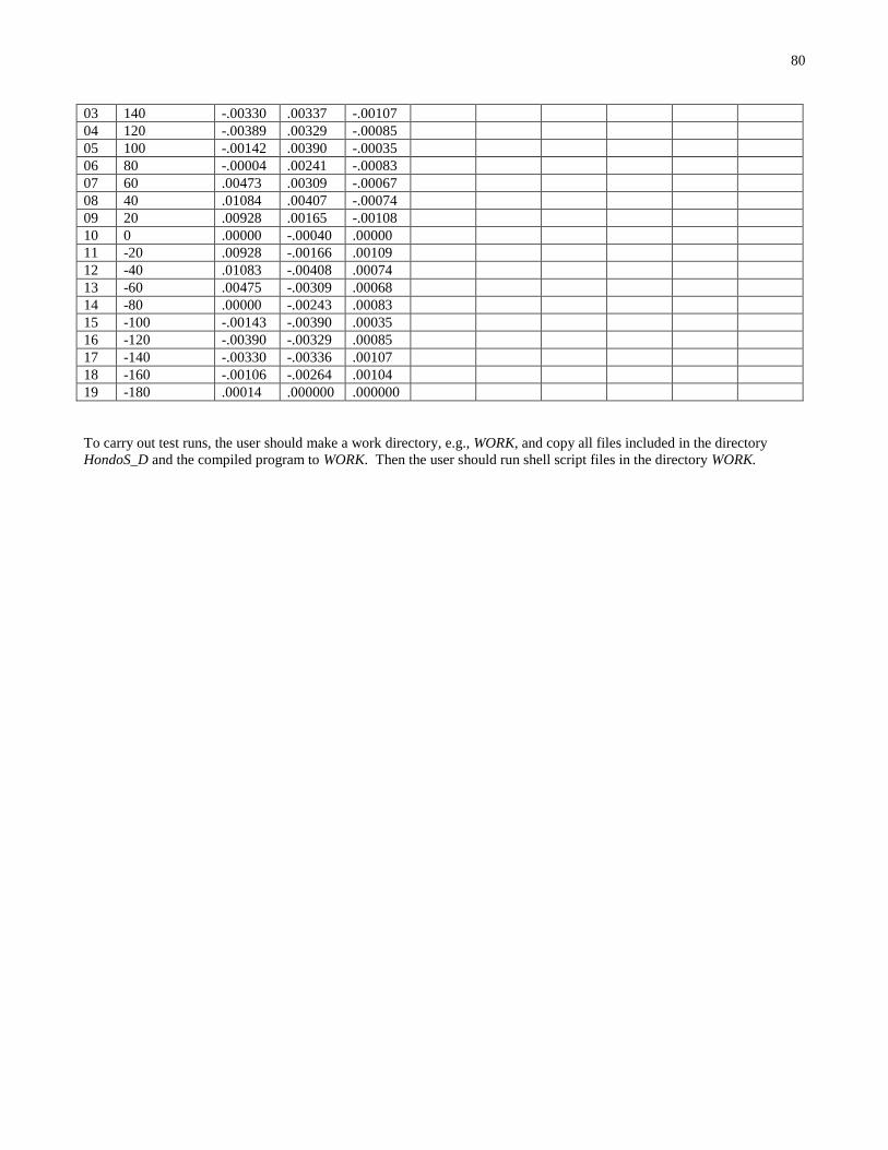
80

03 140 -.00330 .00337 -.00107

04 120 -.00389 .00329 -.00085

05 100 -.00142 .00390 -.00035

06 80 -.00004 .00241 -.00083

07 60 .00473 .00309 -.00067

08 40 .01084 .00407 -.00074

09 20 .00928 .00165 -.00108

10 0 .00000 -.00040 .00000

11 -20 .00928 -.00166 .00109

12 -40 .01083 -.00408 .00074

13 -60 .00475 -.00309 .00068

14 -80 .00000 -.00243 .00083

15 -100 -.00143 -.00390 .00035

16 -120 -.00390 -.00329 .00085

17 -140 -.00330 -.00336 .00107

18 -160 -.00106 -.00264 .00104

19 -180 .00014 .000000 .000000

To carry out test runs, the user should make a work directory, e.g., WORK, and copy all files included in the directory

HondoS_D and the compiled program to WORK. Then the user should run shell script files in the directory WORK.

81

Platforms



HP Cluster Platform 3000 BL280c Red Hat Linux 4.4.6-4 pgf77 version 12.9 makefile.linux

SGI systems SUSE Linux 3.0.13-

0.27

pgf77 version 11.7-0 makefile.linux



IBM pSeries 690 and pSeries 655 AIX version 5.2 XL Fortran version 9.1 makefile.ibm

Netfinitiy Linux cluster Red Hat Linux 2.4.21 pgf77 version 5.2.4 makefile.linux

SGI-Altix Red Hat Linux 2.4.21 gnu g77 version 3.2.3 makefile.linux

SunBlade 2000 UltraSparc III Solaris 9 Sun ONE Studio version 7.1

gnu g77 version 3.3.1

makefile.sun

makefile.sun

Further information

Updated information, when available, will be posted at the University of Minnesota Computational Chemistry Web site:

http://comp.chem.umn.edu/hondoplus.

Acknowledgments

The authors are grateful to Michel Dupuis, M. Aida, Paul Winget, Patton Fast, Yao-Yuan (John) Chuang, and Laura

Masgrau for assistance.

82

HONDOPLUS Revision History

HONDO/S-v.1.0 (June 1999)

Authors: J. Li, G.D. Hawkins, D.A. Liotard, C.J. Cramer, and D.G. Truhlar

This is the first standard version of HONDO/S. HONDO/S–v.1.0 introduced Löwdin population analysis, the CM2 charge

model, and the SM5.42R solvation model to HONDO 99 for wave functions that use Cartesian basis functions. This allowed

for CM2 atomic charge and SM5.42R solvation energy evaluations using HF/MIDI!6D, HF/6-31G*, and HF/6-31+G*.

HONDO/S-v.1.0.1 (May 2000)

Authors: J.D. Xidos, J. Li, G.D. Hawkins, D.A. Liotard, C.J. Cramer, and D.G. Truhlar

The description of the ISCRF option was corrected in this manual (Namelist $SM5, $CM2) and in subroutine SM5HAM.

An error in the evaluation of the N,C(2) surface tension term was corrected.

HONDO/S-v.2.0 (June 2000)

Authors: J.D. Xidos, J. Li, G.D. Hawkins, D.A. Liotard, C.J. Cramer, and D.G. Truhlar

Subroutines SM5CM2, SM5HAM, and SM5S12 were modified to allow for CM2 and Löwdin atomic charge and SM5.42R

solvation calculations involving wave functions that use spherical harmonic d functions. This allows for the

calculation of CM2 and Löwdin atomic charges and of SM5.42R solvation free energies for HF/MIDI!, B3LYP/MIDI!,

and HF/cc-pVDZ.

The N,C(3) surface tension term was added to subroutine SM5STN.

The SM5.42R output printed by HONDO/S now corresponds with that of other codes that implement SM5.42R.

File fld.f was split into two files: fld1.f and fld2.f, where fld2.f contains all of the CM2 and SM5 subroutines that were

originally in fld.f, and fld1.f contains all of the other subroutines that were originally in fld.f.

The Overview of HONDO/S–v.2.0 section was added to the manual, and the Namelist $SM5, $CM2 section was modified.

83

HONDO/S–v.3.0 (May 2001)

Authors: J.D. Xidos, J. Thompson, J. Li, G.D. Hawkins, D. Rinaldi, T. Zhu, D.A. Liotard, C.J. Cramer, and D.G. Truhlar

Analytical gradients and the capability to optimize solute geometries in liquid solutions by the SM5.42/HF/MIDI!6D, and

SM5.42/HF/6-31G* solvation models with ISCRF = 1. Saddle point optimizations and liquid-phase Hessians are not

currently available, however.

The Gauss-Legendre algorithm for the determination of the effective Born radii and their gradients has replaced the force

trapezoid algorithm. A more complete description of the Gauss-Legendre quadrature and its implementation in HONDO/S is

given in “Analytical energy gradients of a self-consistent reaction-field solvation model based on CM2 atomic charges”,

Zhu, T.; Li, J.; Liotard, D. A.; Cramer, C. J.; Truhlar, D. G. J. Chem. Phys. 1999, 110, 5503-5513.

The updating scheme for adding to the Fock operator has been slightly modified. Previous versions of HONDO/S may

have run into problems if it took more than 128 iterations to obtain SCF convergence, and this potential problem has been

eliminated.

The exponent of the outer-valence SP function in the 6-31G* basis set for the sulfur has been changed from 0.0.1195221 to

0.117167 so that it agrees with the published value of Francl, M. M.; Pietro, W. J.; Hehre, W. J.; Binkley, J. S.; Gordon, M.

S.; DeFrees, D. J.; Pople, J. A. J. Chem. Phys. 1982, 77, 3654.

The capability to perform single-point energy + gradient calculations has been added with the addition of the new keyword

GRADIENT in the $JOB data group and with the new RUNFLG option of –3 (i.e. RUNFLG = -3) in the $CNTRL and

$CTL namelists.

A gradient calculation is now performed for the test suite cases test1.xy to test8.xy where x = 0 or 1 and y = 2 or 3. A

geometry optimization of 2,4-pentadione in acetonitrile (test10) has also been added to the test suite.

HONDO/S-v.3.1 (May 2001)

Authors: J. D Xidos, J. Thompson, G. D. Hawkins, J. Li, T. Zhu, B. J. Lynch, D. Rinaldi, D. A. Liotard, C. J. Cramer, and

D. G. Truhlar

.

The mPW exchange functional and the PW91 correlation functional have been added for energies and gradients. Note that

the mPW method in HONDO/S does not have the bug that is in Gaussian98 (see reference LZ03).

The BPW91, MPW1K, and mPW1PW91 methods have been added. These methods can be used by setting the input

variable DFTFUN equal to 7, 8, or 9 respectively.

A subroutine called SCFCLR has been added to the scf.f file. This subroutine prints out additional information during

ONSAGER, QM/MM, and COSMO calculations.

Three test runs have been added: test11.01.in, test11.02.in, and test11.03.in. The test run test11.01.in is an mPW1PW91

optimization of Li2. The test run test11.02.in is a MPW1K optimization of OH. The test run test11.03.in is a BPW91

optimization of OH.

84

HONDO/S-v.3.1.1 (June 12, 2001)


D. G. Truhlar

.

Corrected the implementation of the Mayer bond order for unrestricted wave functions:

In Mayer's well-known paper on bond order (Mayer, I. Chem. Phys. Lett. 1983, 97, 270), the bond order ABB between

atoms A and B is defined as:

PSPSB

A B

AB (1)

where P is the density matrix and S is the overlap matrix, and where basis functions λ and ω reside on atoms A and B,

respectively. This formulation is only correct for restricted wave functions where all orbitals are doubly occupied. Later,

in an addendum and in a full paper (Mayer, I. Chem. Phys. Lett. 1985, 117, 396; Mayer, I. Int. J. Quant. Chem. 1986, 29,

73), Mayer provided a formula for UHF wave functions:

A B

A B

SSAB

2

SPSPSPSP

SPSPSPSPB

(2)

(3)

where P and

P are the alpha and beta spin density matrices, respectively, PPP is the spinless density matrix,

and PPPS is the spin density matrix. Equations (2) and (3) reduce to equation (1) for restricted wave functions.

The implementation of the Mayer bond order matrix for unrestricted wave functions in previous versions of

HONDO/S used the form:

SPPSPP

A B

AB B (4)

The code that calculates CM2 charges in versions of GAMESOL up to version 3.0 and versions of MN-GSM up to version

99.6 also compute the Mayer bond order using equation (4). Equation (4) is correct for restricted wave functions but is

incorrect for unrestricted wave functions. For information sake, we note that the code that calculates population analysis in

GAMESS and HONDO evaluates the Mayer bond order using equation (2) or (3). In version 3.1.1, equations (2) and (3)

have been implemented in the evaluation of bond order for both restricted and unrestricted wave functions, and to evaluate

the contributions of the bond order matrix to the Fock operator and the gradient.

HONDO/S-v.3.2 (June 15, 2001)


D. G. Truhlar

1. Enabled the evaluation of solvation energies and gradients using the Generalized Born model with Löwdin charges

(ICMD = ICDS = 0).

2. Subroutine SM5S12 has been modified to allow the evaluation of Löwdin charges for wave functions that employ

spherical harmonic f functions.

3. The DZVP basis set is provided in the HONDO/S distribution in the file dzvp.bas.

4. The size of the test suite has been increased significantly to in order to test recent enhancements to the HONDO/S

code, including CM2/BPW91 atomic charges, SM5/BPW91 evaluations, Generalized Born solvation model,

liquid-phase numerical frequencies and saddle point optimization, the correct Mayer bond order for unrestricted

wave functions, and Lowdin atomic charges using wave functions that employ spherical harmonic f functions.

85

HONDO/S-v.3.3 (June 18, 2001)

Authors: J.D. Xidos, J.D. Thompson, J. Li, G.D. Hawkins, T. Zhu, B.J. Lynch, Y. Volobuev, D. Rinaldi, D.A. Liotard,

C.J. Cramer, and D. G. Truhlar

The following changes were made to enable HONDO to run on SGI platforms:

System dependent routines were combined into one file, called hondo_ibm.f for IBM systems and hondo_sgi.f for SGI

systems. Specifically, the file aix.f, which contained timing routines, vec.f, which contained a subroutine that performs a

generalized diagonalization were appended to the hnd.f. The file hnd.f now bears the name hondo_ibm.f and hondo_sgi.f.

Additionally, subroutine FIFLSH (from file io.f) and subroutine MQ2FLSH (from file mq2.f) added to hondo_ibm.f and

hondo_sgi.f. These two routines made a call to the FORTRAN routine FLUSH, which is used to write important data to

backup files.

The $MM namelist name has been changed to $MMNOPOL to avoid potential conflicts with the $MMPOL namelist. The

$OPTZ namelist name has been changed to $FREZ to avoid conflicts with the $OPT namelist.

Note also that the $QM namelist must always occur before the $QMMM data group if both are defined in the input.

Similarly, the $GUGDM namelist must always occur before the $GUGDM2 namelist if both are defined in the input.

User-defined density functionals have been added with a modification of the DFTFUN keyword in the $SCF namelist.

Extended test suite to illustrate the use of the new namelist names $FREZ and $MMNOPOL. The test suite has also been

extended to illustrate the new capability of user defined density functionals.

HONDO/S-v.3.3.1 (August 6, 2001)



A bug was fixed for DFT calculations. In particular, it is now possible to apply DFT to one-electron systems.

HONDO/S-v.3.4 (August 6, 2001)



The keywords MIDIX, 6-31GA, 6-31GA*, and 6-31GA** have been added.

SM5.42 parameters for Si have been implemented.

An extended test suite was added to illustrate the new keywords and the newly developed solvation parameters for Si.

Perl scripts have been added to collect data from a major portion of the HONDO/S test suite output for easy comparison to

distributed results.

The debugging flags in the SGI version of the makefile have been removed, making this version of the code run as fast as

the IBM versions.

HONDO/S-v.3.4.1 (January 7, 2002)



The SM5.42 parameters for silicon were changed to their correct values according to “Parameterization of a Universal

Solvation Model for Molecules Containing Silicon”, Winget, P; Thompson, J. D., Cramer, C. J.; Truhlar, D. G. J. Phys.

Chem. B 106, 5160-5168 (2002).

86

HONDO/S-v.3.5 (March 7, 2002)



Update by: J. D. Thompson, H. Nakamura, and D. G. Truhlar

To make HONDO/S more portable, all Fortran 90 code has been removed. This change affects subroutines SM5INP,

SM5SET, SM5ADD, SM5S12, SM5CM2, SAVCM2, SM5MOD, BORNRD, SM5CDS, OSM5, CDSSM5, SM5HAM,

SM5NRG, SM5SOL, DOGEOM, GPDER, BOND_ORDER, MATMUT, S12DER, EXPND1. These routines utilized

several modules, which replaced several common blocks, dynamically allocated local work arrays (i.e., arrays defined only

within that particular subroutine), and used case statements. In addition, subroutine SM5END was removed. This

subroutine was called in subroutine HNDAUT, and it was used to deallocate several arrays at the very end of a given

calculation.

HONDO/S-v.4.0 (March 14, 2002)

Authors: H. Nakamura, J.D. Xidos, J.D. Thompson, J. Li, G.D. Hawkins, T. Zhu, B.J. Lynch, Y. Volobuev, D. Rinaldi,

D.A. Liotard, C.J. Cramer, and D. G. Truhlar

Updates by: H. Nakamura and D. G. Truhlar

A new capability for calculating diabatic states based on configurational uniformity was added. The new capability contains

two main parts:

(1) Diabatization of CASSCF wave functions by the fourfold way. The details of the algorithm are given in "The direct

calculation of diabatic states based on configurational uniformity", H. Nakamura and D. G. Truhlar, J. Chem. Phys. 115

10353 (2001).

(2) Diabatization of MCQDPT wave functions, which include dynamical correlation, by the fourfold way. The details of

the algorithm are given in “Direct diabatization of electronic states by the fourfold way: Including dynamical

correlation and a more general strategy for application to rearrangement processes,” H. Nakamura and D. G. Truhlar, to

be published.

In addition, an extension of the fourfold way was added as an option (H. Nakamura and D. G. Truhlar, unpublished work).

This algorithm allows orbital rotation within separated blocks (DC, VL, VIR) in the fourfold way step. Details are

described in this manual.

The central parts of the routines that provide all of the above capabilities are contained in the new file diab.f. All necessary

calculations for diabatization are performed through subroutines in diab.f. However, CASSCF or MCQDPT calculations

are necessary before diabatization, and handling data obtained by these calculations is also necessary. Therefore the

following subroutines in other files are slightly modified:

(a) HNDCTL (ctl.f): modified to allow WFN = 15,16 in the namelist $WFNFLG; these are options for diabatization

(b) WFNX (wfn.f): modified to allow WFN = 15,16 in the namelist $WFNFLG; these are options for diabatization

(c) MCSCF (ntn.f): a new common block and a parameter were added to store irreps labels of MOs used in routines of

diab.f

(d) MQDRV (mq2.f): a new common block was added to store data to use routines in diab.f. Also a part that calls the

subroutines DIABMQDR and DIABMQWR2 (diab.f) was added to handle data.

To carry out diabatization, two new namelists, $DIABAT and $PROTOTYPE, and three new data groups, $DIAVEC,

$DFMVEC, and $CSFDAT, were introduced and added in the manual.

A new test suite was added to illustrate diabatization scheme.

The part, "Overview of HONDO/S" was separated into the two parts, solvation models (this part of the code is the same as

in version 3.5) and diabatization method (which is the new capability added in this version, 4.0).

87

HONDO/S-v.4.1 (August 29, 2002)



Updates by: J. D. Thompson, C. J. Cramer, and D. G. Truhlar

The CM3 parameter sets, which allow for evaluation of CM3 charges, were added to this version of HONDO/S. This

provides the capability to evaluate gas-phase CM3 charges, liquid-phase CM3 charges, and the electrostatic contribution to

the free energy of solvation using the generalized Born model. The corresponding CM3/GB gradient may also be evaluated

and used for geometry optimizations.

The redistributed Löwdin population analysis (RLPA) method was also added to this version of HONDO/S for two basis

sets that have diffuse functions (6-31+G* and 6-31+G**). This new method can be used to evaluate gas-phase RLPA

charges and liquid-phase RLPA charges for these two basis sets. The RLPA charges can further be used in a calculation of

the electrostatic contribution to the free energy of solvation using the generalized Born model and of the corresponding free

energy gradient, which can also be used for geometry optimizations.

The namelist has been broadened to support the new options as well as the previous ones. The namelist is now called

$HONDOS (although the old names, $CM2 and $SM5, may also be used if desired). To accommodate the new methods,

the allowed values of the ICMD keyword have been extended to include 300, 302, 303, and 315 – 319. Also, the HFE

keyword, which specifies the percentage of HF exchange used in the mPW exchange functional, has been added.

The MG3 and MG3S basis sets were added to HONDO/S. In addition, the keywords MG3 and MG3S were added to the

$BAS data group.

The test suite was extended to test all of the CM3 parameter sets and to test the use of RLPA charges.

HONDO/S-v.4.2 (September 6, 2002)




The CM3 parameter sets for the BLYP and B3LYP methods were added to this version of HONDO/S. This provides the

capability to evaluate gas- and liquid-phase charges and the electrostatic contribution to the free energy of solvation using

the generalized Born model. The corresponding CM3/GB gradient may also be evaluated.

The keyword ICMD was extended to allow values of 313, 314, 320, and 321 to accommodate the new methods.

The test suite was extended to test the new CM3 parameter sets.

HONDO/S-v.4.3 (January 8, 2003)




The algorithm of diabatization, “fourfold way”, was improved by introducing “pre-fourfold way” procedure.

HONDOPLUS-v.4.3 (April 7, 2003)




The name of the program was changed.

88

HONDOPLUS-v.4.4 (August 29, 2003)




The program was ported to machines running the RedHat Linux operating system. This involved grouping

system-dependent routines into a new source file, hondo_linuf.f and creating a new makefile, makefile.linux.

HONDOPLUS-v.4.4.1 (March 12, 2004)




The dimensions of arrays DCOTDR in subroutine CDSSM5 and FGB in subroutine SM5CDS were incorrect. Instead of

having dimensions of MXATM*(MXATM+1)/2, where MXATM = 128, they had dimensions of MXATM. So molecules

larger than 15 atoms would cause these two arrays to spill into other arrays. We have observed erroneous results for a

liquid-phase geometry optimization of a 19 atom molecule. The dimensions of DCOTDR and FGB have been corrected.

HONDOPLUS-v.4.5 (March 17, 2004)




The SM5.43R and SM5.43 solvation models were added. In particular, parameter sets for HF/6-31G*, B3LYP/6-31G*,

mPW1PW91/6-31G*, and mPW1PW91/6-31+G* were added. The test suite was updated to test these new models.

Modifications to subroutines SM5INP, SM5SET, DOSOLV, COULRD, SM5STN, and OSM5 were made.

HONDOPLUS-v.4.6 (July 28, 2004)




Additional parameter sets for the SM5.43R and SM5.43 solvation models were added. In particular, the SM5.43R and

SM5.43 parameters for MPWX/MIDI!, MPWX/MIDI!6D, MPWX/6-31G(d), MPWX/6-31+G(d), and MPWX/6-31+G(d,p),

where X can take on any value between 0 and 60.6, were added. The test suite was updated to test these new models.

Modifcations to subroutines SM5INP, SM5SET, SM5STN, and OSM5 were made.

HONDOPLUS-v.4.7 (July 28, 2005)

Authors: H. Nakamura, J.D. Xidos, C.P. Kelly, J.D. Thompson, J. Li, G.D. Hawkins, T. Zhu, B.J. Lynch, Y. Volobuev, D.

Rinaldi, D.A. Liotard, C.J. Cramer, and D. G. Truhlar

Updates by: C.P. Kelly, C. J. Cramer, and D. G. Truhlar

The parameters sets for CM3/HF/MIDI! and CM3.1/HF/MIDI! have been added. CM3.1 is designed to give accurate

charges for high-energy materials.

The parameters sets for CM4/DFT/MIDI!6D, CM4/DFT/6-31G(d), CM4/DFT/6-31+G(d), and CM4/DFT/6-31+G(d,p),

where DFT is any good density functional, have been added.

The parameters sets for SM6/DFT/MIDI!6D, SM6/DFT/6-31G(d), SM6/DFT/6-31+G(d), and SM6/DFT/6-31+G(d,p) have

been added.

The section entitled “Density Functional Methods Recommended for use with CM4 and SM6 in HONDOPLUS–v4.7” has been

added. This section gives a description of the functionals in HONDOPLUS–v4.7 that are recommended for use with SM6.

89

The keywords IRADII and ISTS was added. The IRADII keyword specifies the set of atomic-number-dependent radii that

are used to build the molecular cavity. The ISTS keyword determines whether SM5- or SM6-type functionals are used.

Coulomb radii are now defined for all atoms on the periodic table. In the past, atoms whose Coulomb radii were not

optimized as part of a given solvent model were assigned default values of 0 Å. In HONDOPLUS–v4.7, atoms whose

Coulomb radii have not been optimized are assigned a radius equal to Bondi’s value for the van der Waal’s radius. Atoms

for which Bondi has not assigned atomic radii to are assigned a value of 2.0 Å. Thus, Generalized Born calculations can be

carried out for molecules containing any element on the periodic table.

The keyword SolvRd was added. This keyword allows the user to specify a value for the solvent radius, which is used for

the calculation of the solvent-accessible surface areas of the atoms of the solute.

The “R” notation used by SM5.42 and SM5.43 to distinguish single-point solvation calculations based on rigid gas-phase

geometries from liquid-phase geometry optimizations has been dropped for all models. The Pople style notation (i.e.

level/basis//level/basis) is now used.

HONDOPLUS-v.4.8 (September 2, 2005)




For methods that use diffuse basis functions, ISCRF = 1 (SCF Scheme I) is no longer available due to convergence

problems.

An extended test suite for SM6 has been added. The input and output files for this portion of the test suite are located under

the directory /sm6.

HONDOPLUS-v.4.9 (November 17, 2005)




The code is now compatible with with the gnu g77 compiler.

HONDOPLUS-v.5.0 (November 17, 2005)

Authors: H. Nakamura, J.D. Xidos, A.C. Chamberlin , C.P. Kelly, J.D. Thompson, J. Li, G.D. Hawkins, T. Zhu, B.J.

Lynch, Y. Volobuev, D. Rinaldi, D.A. Liotard, C.J. Cramer, and D. G. Truhlar

Updates by: A. C. Chamberlin, C. J. Cramer, and D. G. Truhlar

Minor corrections to the code were implemented.

The atomic surface tensions used to compute the temperature dependence of the free energy of solvation have been added.

A new keyword (SolK) has been added to read in the temperature of a liquid aqueous solution and to compute free energies

of solvation at the given temperature. The keyword only accepts values within the range of 273 to 373 K

A new keyword (ReadK) has been added to read in temperatures from a file named ‘Temperatures’ and to compute free

energies of solvation for a particular molecule in aqueous solution. Note that this approach uses the solution-phase

electronic structure as an initial guess for successive temperatures, so one may obtain identical electronic energies if the

temperatures are very near to one another. To avoid this either use very strict convergence criteria, or do not order similar

temperatures very near one another. The differences in electronic energies are very small anyway.

90

Another keyword (AvgK) which is similar to ReadK computes the electrostatics by computing the electronic energy of the

solute in solution at the average of all the temperatures in the file ‘Temperatures’ and then uses a scaling factor to compute

the electronic energy at a given temperature. Note that this option is considerably faster than the ReadK option.

An additional test suite for SM6T has been added. The input and output files are located in hondoplus-v5.0/HondoS/sm6t/

HONDOPLUS-v.5.1 (February 17, 2007)

Authors: H. Nakamura, J.D. Xidos, A.C. Chamberlin , C.P. Kelly, R. Valero, J.D. Thompson, J. Li, G.D. Hawkins, T. Zhu,

B.J. Lynch, Y. Volobuev, D. Rinaldi, D.A. Liotard, C.J. Cramer, and D. G. Truhlar

Updates by: R. Valero and D. G. Truhlar

The intruder state avoidance (ISA) method has been implemented. The original code has been taken from the GAMESS

program with permission from Professor Mark Gordon, Ames Laboratory, Iowa State University. A new keyword EDSHFT

has been added to the $MCQDPT namelist. Note that only the non-relativistic part (i.e., without spin-orbit terms) of the

ISA method as implemented in GAMESS has been introduced into HONDOPLUS-v5.1.

In HONDOPLUS-v5.1, an option is added to exclude the ground state from the fourfold way procedure. In this case, only

the N-1 excited adiabatic states and energies are transformed to the diabatic representation. The keyword NGRSTATE has

been added to the $DIABAT namelist and allows to run fourfold way calculations with or without the ground state included.

The fourfold way now runs on non-IBM as well as IBM machines. The list of machines tested includes IBM Power 4

Regatta, Netfinity (Redhat Linux, pgf77 compiler), SGI Altix (Redhat Linux), and SunBlade 2000 (Solaris 9).

HONDOPLUS-v.5.2 (January 15, 2013)

Authors: H. Nakamura, J.D. Xidos, A.C. Chamberlin , C.P. Kelly, R. Valero, K.R. Yang, J.D. Thompson, J. Li, G.D.

Hawkins, T. Zhu, B.J. Lynch, Y. Volobuev, D. Rinaldi, D.A. Liotard, C.J. Cramer, and D. G. Truhlar

Updates by: K.R. Yang and D. G. Truhlar

A new scheme has been added to the fourfold way diabatization of MC-QDPT wave functions with CASSCF DMOs. See

K.R. Yang, X. Xu, and D.G. Truhlar, Chem. Phys. Lett., submitted.

91

Data Group $JOB

Function

This data group provides an easy, shorthand specification of key parameters defining a run. There are only four different

types of input parameters, each taking on a limited number of assignments. They are: a. a wave function selection

parameter, b. an automated procedure selection parameter, and lastly c. three parameters related to the use of symmetry, to

the calculation of molecular properties, and to the selection of the computational algorithm (standard, semi-direct, direct).

Parameters

Wave function selection

HF Hartree-Fock wave function and energy

MP2 MP2 energy

MP4 MP4 energy

Automated Procedure selection

ENERGY energy calculation

GRADIENT calculation of the energy and the gradient of the energy

OPT optimization

FORCE second derivative calculation

FREQ frequency calculations

SADDLE transition state calculation

LST Linear Synchronous Transit Pathway calculation

NLO Finite-Field (hyper)polarizability calculation

Property selection

NOPROP do not calculate molecular properties

Symmetry selection

NOSYM do not make use of point group symmetry Algorithm selection

Algorithm selections (default is: 'standard-with-disk' when no algorithm parameter is specified)

SEMI-D use 'semi-direct algorithm'

DIRECT use 'direct' algorithm

Comments

One and only one wave function parameter may be specified. One and only one automated procedure parameter may be

specified. One and only one algorithm parameter may be specified. The other two parameters are optional.

92

Data Group $BAS

Function

This data group provides a means to specify a global basis set name, when all the atoms in the molecule all carry basis sets

of a single type. Or else it is a means to assign external basis sets to each atom. When specifying a global basis set name,

that name must be one of the standard ‘internal’ basis set names stored in the code. When specifying ‘external’ basis sets,

the data group $BAS must include at least as many names as there are atoms specified in the data group $GEO. In that case

the names can be either those of standard ‘'internal’ basis sets or names of ‘external’ basis sets which then must be included

in the input data. Additionally, the ‘basis set’ name can be DUMMY, which applies to ‘dummy’ atoms as specified in

$GEO.

The standard names are:

STO, STO-3G,

3-21G, 6-21G, 6-21G*, 6-21G**, 4-31G,

6-31G, 6-31G*, 6-31G**,

6-31GA, 6-31GA*, 6-31GA**,

DZV, DZP, TZV, TZP, ECDZ, ECDP, ECTZ, ECTP,

MINI, MIDI, MIDIX, MG3, and MG3S

External basis sets are specified by a group of data similar to those needed to define external basis sets in $BASIS data

group. Each set of data comprises a header card which has the format ‘$name’, followed by the shell and primitive

Gaussian data, terminated with a ‘$END’ data card.

Comments

As an example, the following record requests the 6-31G basis set for all the atoms on the molecule:

$BAS 6-31G $END

Another example would be for C2H4 molecule in which the atoms are entered through $GEO in the order C, C, H, H, H, H:

$BAS STO-1 STO-1 STO-0 STO-0 STO-0 STO-0 $END

$STO-1

1 1S 3 STO

2 2SP 3 STO

$END

$STO-0

1 1S 3 STO

$END

The two carbon atoms have the basis set STO-1 assigned to them, while basis set STO-0 is assigned to all the H atoms.

Basis set STO-1 is defined in records 2 through 6, while basis set STO-0 is defined in records 7 through 10. If a ‘dummy’

atom is specified in $GEO (with an atom name of X or Bq), then the basis name given for this atom should be DUMMY as

in the example below where the atoms are C, X, C, H, H, H, H:

$BAS BAS-C, DUMMY, BAS-C, BAS-H, BAS-H, BAS-H, BAS-H, $END

$BAS-C

1 SV 6 N31

2 D 1

1 0.8 1.0

93

$END

$BAS-H

1 SV 6 N31

$END

Note that the program will automatically assign an 'empty' basis set to a 'dummy' atom, so that an equally valid data would

have been:

$BAS 6-31G*, $END

The code will understand that all the atoms will have the 6-31G* basis set, and will give no basis functions to the 'dummy'

atom. What the program will not let you do, is specify an atom with its full atomic charge for which you ask for a 'dummy'

basis.

$BAS 6-31G, DUMMY, 6-31G, STO-3G, STO-3G, STO-3G, STO-3G, $END

This ought to be done by means of $EFC.

A working example with dummy atoms is as follows:

$JOB HF ENERGY NOPROP $END

$BAS 6-31G, $END

$GEO

H2O, 6-31G

O

X 1 1.0

H 1 R1 2 theta1

H 1 R1 2 theta1 3 phi1

R1 = 1.04

theta1 = 125.0

phi1 = 180.0

$END

Another form of it would be:


$BAS BAS-O, DUMMY, BAS-H, BAS-H, $END

$GEO

H2O, 6-31G

O

X 1 1.0

H 1 R1 2 theta1


R1 = 1.04

theta1 = 125.0

phi1 = 180.0

$END

$BAS-O

1 SV 6 N31

$END

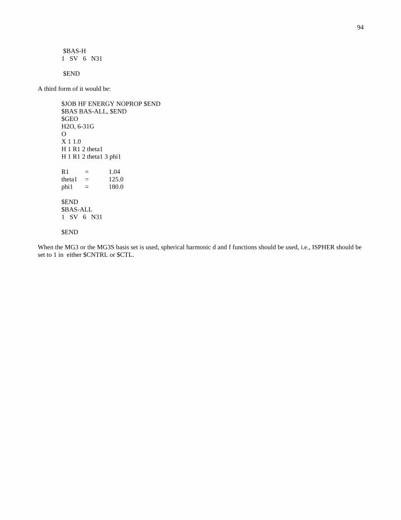
94

$BAS-H

1 SV 6 N31

$END

A third form of it would be:


$BAS BAS-ALL, $END

$GEO

H2O, 6-31G

O

X 1 1.0

H 1 R1 2 theta1


R1 = 1.04

theta1 = 125.0

phi1 = 180.0

$END

$BAS-ALL

1 SV 6 N31

$END

When the MG3 or the MG3S basis set is used, spherical harmonic d and f functions should be used, i.e., ISPHER should be

set to 1 in either $CNTRL or $CTL.

95

Namelist $BASINP

Function

This namelist allows to specify the basis set input parameters such as NORMF, NORMP, ITOL, and IUNIT found in

$BASIS. See that data group description for information.

Parameters

NORMF basis function normalization option (default = 0)

0 … normalize basis functions

1 … do not normalize basis functions

NORMP primitive Gaussian normalization option (default = 0)

0 … normalize primitive Gaussian functions

1 … do not normalize primitive Gaussian functions

ITOL pre-exponential tolerance parameter (default = 0)

IUNIT flag defining units (bohr or Å) in $GEO (default = 1; units are Å)

-1 … units are a.u.

… internal coordinates (see $BASIS)

… units are Å

GEOFIL unix file name for reading coordinates from a biosym.car file (default = blank)

IECP flag to indicate that Effective Core Potentials (ECP) must be read from the input file

(default = 0)

0 … no $ECP input to be read in

1 … read $ECP in input stream

Comments

See $BASIS data input for definition of parameters.

The following biosym.hnd input file for HONDO which contains the single input line below, makes the code read the

coordinates from biosym.car created with Biosym's DISCOVER graphical interface, and then the code executes a STO-3G

SCF calculation, as a result of all the defaults:

$BASINP GEOFIL='biosym.car', $END

Other parameters can be defined as usual beyond this.

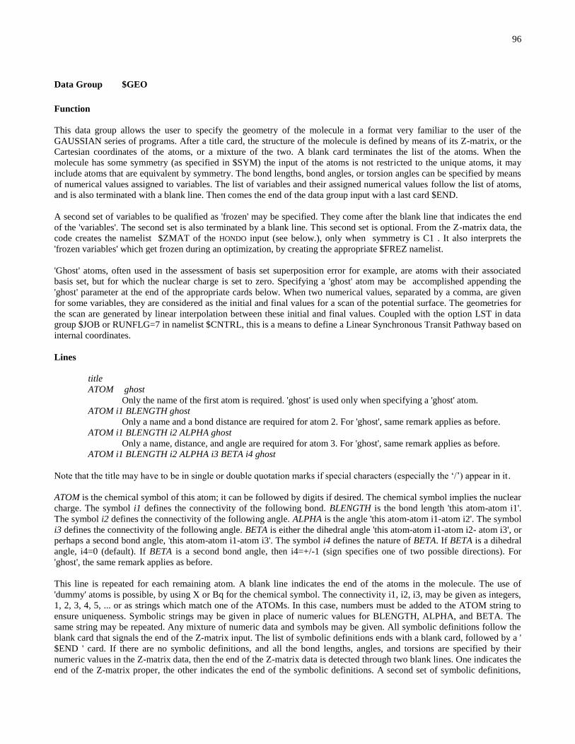
96

Data Group $GEO

Function

This data group allows the user to specify the geometry of the molecule in a format very familiar to the user of the

GAUSSIAN series of programs. After a title card, the structure of the molecule is defined by means of its Z-matrix, or the

Cartesian coordinates of the atoms, or a mixture of the two. A blank card terminates the list of the atoms. When the

molecule has some symmetry (as specified in $SYM) the input of the atoms is not restricted to the unique atoms, it may

include atoms that are equivalent by symmetry. The bond lengths, bond angles, or torsion angles can be specified by means

of numerical values assigned to variables. The list of variables and their assigned numerical values follow the list of atoms,

and is also terminated with a blank line. Then comes the end of the data group input with a last card $END.

A second set of variables to be qualified as 'frozen' may be specified. They come after the blank line that indicates the end

of the 'variables'. The second set is also terminated by a blank line. This second set is optional. From the Z-matrix data, the

code creates the namelist $ZMAT of the HONDO input (see below.), only when symmetry is C1 . It also interprets the

'frozen variables' which get frozen during an optimization, by creating the appropriate $FREZ namelist.

'Ghost' atoms, often used in the assessment of basis set superposition error for example, are atoms with their associated

basis set, but for which the nuclear charge is set to zero. Specifying a 'ghost' atom may be accomplished appending the

'ghost' parameter at the end of the appropriate cards below. When two numerical values, separated by a comma, are given

for some variables, they are considered as the initial and final values for a scan of the potential surface. The geometries for

the scan are generated by linear interpolation between these initial and final values. Coupled with the option LST in data

group $JOB or RUNFLG=7 in namelist $CNTRL, this is a means to define a Linear Synchronous Transit Pathway based on

internal coordinates.

Lines

title

ATOM ghost

Only the name of the first atom is required. 'ghost' is used only when specifying a 'ghost' atom.

ATOM i1 BLENGTH ghost

Only a name and a bond distance are required for atom 2. For 'ghost', same remark applies as before.

ATOM i1 BLENGTH i2 ALPHA ghost

Only a name, distance, and angle are required for atom 3. For 'ghost', same remark applies as before.

ATOM i1 BLENGTH i2 ALPHA i3 BETA i4 ghost

Note that the title may have to be in single or double quotation marks if special characters (especially the ‘/’) appear in it.

ATOM is the chemical symbol of this atom; it can be followed by digits if desired. The chemical symbol implies the nuclear

charge. The symbol i1 defines the connectivity of the following bond. BLENGTH is the bond length 'this atom-atom i1'.

The symbol i2 defines the connectivity of the following angle. ALPHA is the angle 'this atom-atom i1-atom i2'. The symbol

i3 defines the connectivity of the following angle. BETA is either the dihedral angle 'this atom-atom i1-atom i2- atom i3', or

perhaps a second bond angle, 'this atom-atom i1-atom i3'. The symbol i4 defines the nature of BETA. If BETA is a dihedral

angle, i4=0 (default). If BETA is a second bond angle, then i4=+/-1 (sign specifies one of two possible directions). For

'ghost', the same remark applies as before.

This line is repeated for each remaining atom. A blank line indicates the end of the atoms in the molecule. The use of

'dummy' atoms is possible, by using X or Bq for the chemical symbol. The connectivity i1, i2, i3, may be given as integers,

1, 2, 3, 4, 5, ... or as strings which match one of the ATOMs. In this case, numbers must be added to the ATOM string to

ensure uniqueness. Symbolic strings may be given in place of numeric values for BLENGTH, ALPHA, and BETA. The

same string may be repeated. Any mixture of numeric data and symbols may be given. All symbolic definitions follow the

blank card that signals the end of the Z-matrix input. The list of symbolic definitions ends with a blank card, followed by a '

$END ' card. If there are no symbolic definitions, and all the bond lengths, angles, and torsions are specified by their

numeric values in the Z-matrix data, then the end of the Z-matrix data is detected through two blank lines. One indicates the

end of the Z-matrix proper, the other indicates the end of the symbolic definitions. A second set of symbolic definitions,

97

separated from the first set through a blank card, may be included to specify frozen internal coordinates. A blank card again

defines the end of the list of 'frozen' internal coordinates.

Note that atoms in the Z-matrix data may be specified via Cartesian coordinates expressed in units of Å, Each line has the

following form:

ATOM X Y Z ghost

ATOM is the atomic name as before, X, Y, Z being the Cartesian coordinates, and ghost is used only when specifying a

'ghost' atom.

Examples

The following example is for a 6-31G SCF calculation on CH3CF3, with all specified angles frozen to the given value :

$BAS 6-31G $END

$GEO

Z-matrix input = CH3-CF3

C

C 1 CC

H 1 CH1 2 HCH1

H 1 CH2 2 HCH2 3 TOR1 +1

H 1 CH3 2 HCH3 3 TOR2 -1

F 2 CF1 1 CCF1 3 TOR30

F 2 CF2 1 CCF2 6 FCH11

F 2 CF3 1 CCF3 6 FCH2 -1

CC= 1.4888

CH1= 1.0790

CH2= 1.0789

CH3= 1.0789

CF1= 1.3667

CF2= 1.3669

CF3= 1.3669

HCH1 = 109.5428

HCH2 = 109.5474

HCH3 = 109.5475

CCF1 = 112.0713

CCF2 = 112.0341

CCF3 = 112.0340

TOR1 = 109.3996

TOR2 = 109.3997

TOR3 = 180.0000

FCH1 = 106.7846

FCH2 = 106.7842

$END

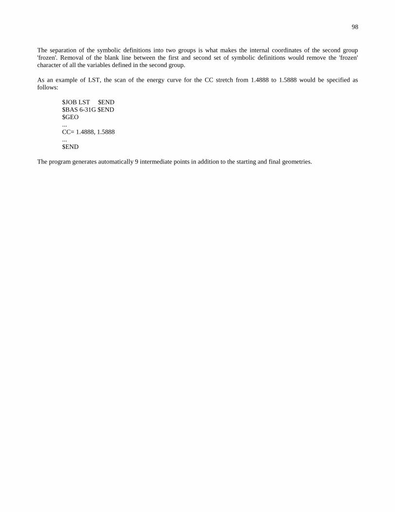
98

The separation of the symbolic definitions into two groups is what makes the internal coordinates of the second group

'frozen'. Removal of the blank line between the first and second set of symbolic definitions would remove the 'frozen'

character of all the variables defined in the second group.

As an example of LST, the scan of the energy curve for the CC stretch from 1.4888 to 1.5888 would be specified as

follows:

$JOB LST $END

$BAS 6-31G $END

$GEO

...

CC= 1.4888, 1.5888

...

$END

The program generates automatically 9 intermediate points in addition to the starting and final geometries.

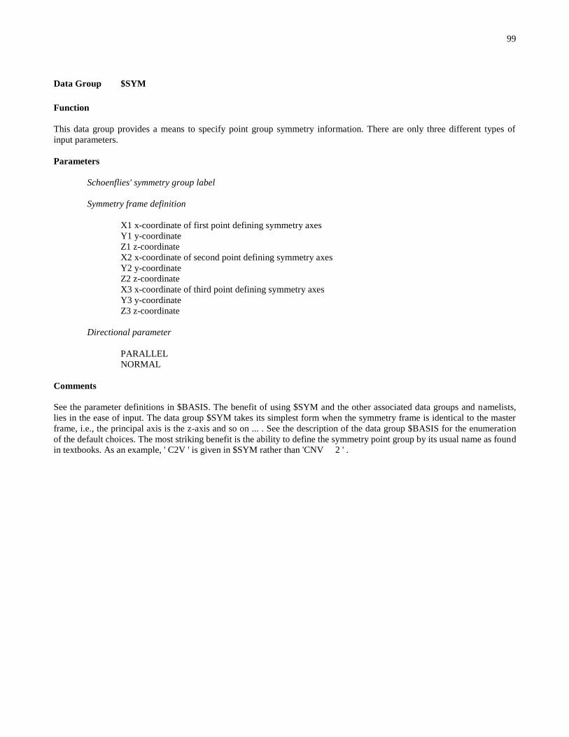
99

Data Group $SYM

Function

This data group provides a means to specify point group symmetry information. There are only three different types of

input parameters.

Parameters

Schoenflies' symmetry group label

Symmetry frame definition

X1 x-coordinate of first point defining symmetry axes

Y1 y-coordinate

Z1 z-coordinate

X2 x-coordinate of second point defining symmetry axes

Y2 y-coordinate

Z2 z-coordinate

X3 x-coordinate of third point defining symmetry axes

Y3 y-coordinate

Z3 z-coordinate

Directional parameter

PARALLEL

NORMAL

Comments

See the parameter definitions in $BASIS. The benefit of using $SYM and the other associated data groups and namelists,

lies in the ease of input. The data group $SYM takes its simplest form when the symmetry frame is identical to the master

frame, i.e., the principal axis is the z-axis and so on ... . See the description of the data group $BASIS for the enumeration

of the default choices. The most striking benefit is the ability to define the symmetry point group by its usual name as found

in textbooks. As an example, ' C2V ' is given in $SYM rather than 'CNV 2 ' .

100

Namelist $CNTRL , $CTL

Function

This namelist defines the major options concerning the run.

Parameters

RUNFLG run type (default = 0)

-3 .... energy + gradient

0 .... energy + properties

1 .... geometry optimization

2 .... force constant calculation

3 .... saddle point determination

4 .... reaction path -IRC- determination

5 .... properties calculation except (hyper)polarizabilities

6 .... dipole and polarizability derivatives

7 .... potential energy surface scan

8 .... non-gradient energy minimization

9 .... minimum energy crossing seam determination

10 .... electron coupling matrix element VA B

11 .... (hyper)polarizability calculation by finite field

12 .... limited geometry optimization (inactive)

13 .... molecular dynamics trajectory driver

14 .... dynamic reaction path -DRC- determination (inactive)

15 .... potential energy surface with -BSSE- correction (inactive)

IREST restart flag (default = 0)

0 .... normal start

1 .... restart during one- or two-electron integrals (OEI , TEI)

2 .... restart during self-consistent-field calculation (SCF)

3 .... restart during one-electron integral derivatives (OEIDER)

4 .... restart during two-electron integral derivatives (TEIDER)

NOPROP flag to prevent calculation of electronic properties (default = 0)

0 .... calculate properties

1 .... do not calculate properties.

NOSYM flag to deactivate point group symmetry for energy and energy derivatives calculation (default =

0)

0 .... use symmetry as given in $BASIS

1 .... deactivate symmetry when necessary

AUTSYM to activate automatic detection of symmetry

(default = 0)

0 …. Do not activate automatic detection of symmetry

1 …. Activate automatic detection of symmetry.

TIME internal time limit in seconds. (default value = 99999.0)

IPRINT print flag (default = 0)

101

0 .... normal output

1 .... debug printing in molecular input (MOLECULE)

2 .... debug printing in initial guess (GUESS)

3 .... debug printing in one electron integrals (OEI)

4 .... debug printing in two electron integrals (TEI)

5 .... debug printing in wave function calculation (WFN)

6 .... debug printing in property calculation (PRP)

-3 .... debug printing in one electron integral derivatives (OEIDER)

-4 .... debug printing in two electron integral derivatives (TEIDER)

-5 .... reduced printing

LIST flag defining the printing format for the molecular orbitals and other matrices;

Used in conjunction with PRTTHR (default = 0)

0 .... usually 10 vectors across (F11.5format)

1 .... usually 7 vectors across (F15.10 format)

2 .... usually 7 vectors across (E15.8format)

PRTTHR threshold for printing elements of a matrix

(default = 0.15)

MODDIA flag to select matrix diagonalization routine. The choice is between

GIVEIS and GIVENS. See source code for information. (default = 1).

0 .... use GIVENS

1 .... use GIVEIS

QMTTOL threshold for linear dependency of canonical orthonormal orbitals

(default = 1.0E-04)

MAXLCM size of common block /LCM/ . It is used to keep the integrals in memory

or to sort the supermatrices (default = MAXLCM defined in CTL.f or VEC.f)

MAXVEC size of array carved out from the common block /SCM/ to handle vector

processing (default = 200000).

MAXXIO size of array carved out from the common block memory resident I/O

(not active , default = 1).

IGRAF flag to punch out data on -FT07- for graphical display (default = 0)

0 .... no special punch-out

1 .... special punch-out

ISPHER flag to keep only the spherical harmonic functions in d , f , and g shells.

(default = 0)

-1 .... use all cartesian components

0 .... use all cartesian components (see below for meaning).

1 .... use only spherical harmonic functions.

102

DIRECT flag to use the direct approach where implemented (RHF, UHF, MCSCF,

and MP2 only) (default = 0).

0 .... use traditional approach

1 .... use direct approach

2 .... use semi-direct approach (see below).

3 .... use semi-direct approach (s, p integrals to disk).

Comments

TIME is the internal time limit (in seconds) against which the CPU time is compared. The run stops when the CPU time of

the job is greater than TIME.

IPRINT is a print (or debug) flag that applies to some program modules. More debug flags are available from other

individual namelists.

IREST is a restart flag. Values of 0 and 1 are safe for all wave functions. Values of 2, 3, and 4 probably work for RHF,

UHF, and GVB wave functions, but do not work for MCSCF and CI wave functions.

RUNFLG indicates the type of run being done (energy calculation, geometry optimization ...).

NOPROP is used to skip the calculation of electronic properties. Another way of achieving the same goal is to define

appropriately the parameters in the namelist $PRP.

NOSYM is used to deactivate the point group symmetry option. Normally the program turns symmetry off when

appropriate, for example when an external field is applied , or for MCSCF or CI calculations with non-abelian point groups.

The reason for turning symmetry off for MCSCF and CI calculations is that when symmetry is active, a reduced list of

electron repulsion integrals are calculated in the atomic orbital basis. The integral transformation program can not handle

the petite list, if the point group contains degenerate irreducible representations. Finally this option is also useful for

debugging purposes. However, the action of turning symmetry off takes place only after the molecular input has been read

in. It may have been read in with explicit symmetry information (see $BASIS), the program generating automatically

symmetry equivalent atoms and atomic basis sets. When NOSYM = 1all of this is still done, and then symmetry gets

deactivated. Finally, note that NOSYM should be set equal to 1 for (hyper)polarizability calculations.

QMTTOL is a threshold used in defining the linear dependency of the canonical orthonormal orbitals. The default value is

adequate for all wave functions. Looser thresholds are quite permissible for SCF wave functions. For correlated energy

calculations looser thresholds than the default value often result in numerical inaccuracies.

The default use of the diagonalization routine GIVEIS is usually adequate. The routine is faster than GIVENS , and

therefore its use is advantageous. However there are cases where GIVEIS seems to end abnormally. It may then be useful to

try the other option. In some cases the program seemed to work well with GIVENS.

MAXVEC: Most of the subroutines in VEC make use of some working area which is defined at the bottom of the common

block /SCM/ . If there is not enough space the program stops. The default allocation appears to be large enough to handle

large basis sets. Some users may want to use a smaller value if they do not make use of vector processing.

DIRECT: This parameter controls the SCF methodology, traditional (DIRECT = 0) or direct (DIRECT = 1), for closed shell

RHF, open shell UHF, CASSCF and MCSCF wave functions, for the MP2 and UMP2 energies and MP2 gradients, for

RHF second derivatives, and for static and dynamic (hyper)polarizabilities. In the direct case the program performs no I/O

but consumes more CPU time than the traditional approach.

The semi-direct (DIRECT = 2) approach implemented for RHF and UHF calculations, and for static and dynamic

(hyper)polarizabilities, stores only some of the integrals on disk and recompute the others as needed. This is used in

conjunction with the parameters THIME, THIZE, and MBYTES in namelist $INTGRL. THIME is a cost factor defining

which integrals are stored on disk. Integrals whose cost is greater than THIME are stored on disk, all others are recomputed

as needed. THIME = 0is equivalent to a standard algorithm (DIRECT = 0). THIME = 10000 () is equivalent to the direct

103

algorithm (DIRECT = 1). THIZE is a size factor, defining which integrals get stored on disk, those whose magnitude

estimates are greater than THIZE. An alternate way is to give the disk space size available for the electron repulsion

integrals in MBYTES, and the code will proceed in semi-direct mode using that amount of disk and no more.

DIRECT = 3 also invokes a semi-direct algorithm whereby the integrals for 's' and 'p' functions are stored on disk and any

other integrals are recomputed as needed. This is a variant of the semi-direct approach described above.

IGRAF: This flag controls some of the punched-out data specially generated for display with the graphical interface

KGNGRAF

ISPHER: This parameter is used to eliminate the unwanted basis functions of d , f , and g shells. The energy calculation is

carried out in the truncated space. This option is often useful when using very large basis set and these unwanted basis

functions may be responsible for linear dependencies in the basis set.

When ISPHER = -1, the program works with the original Cartesian basis functions, from which it constructs the

symmetry-adapted linear combination basis functions which are then used throughout the program, if symmetry is present.

When ISPHER = 0 , the program creates symmetry-adapted linear combinations of the 'local' spherical harmonic functions,

which are then expressed in terms of Cartesian functions. All the functions associated with each shell are kept. When

ISPHER = +1, the program proceeds as in the case of ISPHER = 0, but the 'local' spherical harmonic space is truncated to

eliminate the 3S(D), the 3P(F), the 4S(G), and 3D(G), before creating the symmetry-adapted functions. It is clear then that

the -SALC- functions created when ISPHER = 0, are not identical to the -SALC- functions when ISPHER = -1. The former

are linear combinations of the latter, but the variational space is the same. Thus the energy is the same in both cases. The

option ISPHER = -1 is fully equivalent to what older versions of the code did.

104

Data group $BASIS

Function

This fixed format input group defines the molecular geometry and the basis set. The data group can be read in as well in

free-format, line by line, provided that all parameters are specified specifically. See the paragraph input in the previous

section.

Lines

LINE 1 TITLE(10)

FORMAT(10A8)

LINE 2 NORMF,NORMP,ITOL,IUNIT,IBASIS,IECP,BLKTYP

FORMAT(4I5,1X,A4,1X,A4,2X,A8)

NORMF Flag for normalization of basis functions. (default = 0)

0 ... normalize the basis functions.

1 ... no normalization required.

NORMP Flag for normalization of primitive gaussian functions. (default = 0)

1 ... no normalization; the contraction coefficients correspond to unnormalized

primitive functions.

0 ... normalization required; the contraction coefficients correspond to normalized

primitive functions. In this case, the contraction coefficients of the d, f, g-type primitive

functions should be the ones for the dxx, fxxx, gxxxx primitives. Note that in both cases

(NORMP = 0 or 1) the coefficients of the molecular orbitals are given in terms of

unnormalized primitives, and that in the case NORMF = 0, the coefficients of the

molecular orbitals are given in terms of normalized basis functions.

ITOL Preexponential threshold parameter (default = 15)

The products of primitives with preexponential factor exp(-G) less than 10-ITOL

are

skipped.

IUNIT Flag to specify the unit used to input the atomic coordinates.

+1 ... for Å

0 ... for input of internal coordinates

-1 ... for atomic units

IBASIS Basis set label when a standard basis set is used. Possible labels are:

STO ... for STO-3G basis set

N21 ... for 3-21G basis set

N31 ... for 4-31G basis set

3-21G ... for 3-21G basis set


6-31G ... for 6-31G basis set (used in GAUSSIAN for Si and the third

row)


6-21G* ... for 6-21G* basis set

6-31G* ... for 6-31G* basis set (used in GAUSSIAN for Si and the

third row)

6-21G** ... for 6-21G** basis set

105

6-31G** ... for 6-31G** basis set (used in GAUSSIAN for Si and the

third row)

6-31GA … for 6-31G basis set (Gordon’s version for Si, Pople and

Curtiss’ version for third row atoms)

6-31GA* … for 6-31G basis set (Gordon’s version for Si, Pople and


6-31GA** … for 6-31G basis set (Gordon’s version for Si, Pople and


DZV ... for Dunning's (9s,5p)/(3s,2p) basis set

DZP ... same as DZV above, but with polarization

TZV ... for triple zeta basis

TZP ... for triple zeta plus polarization

ECDZ ... for Compact ECP with double zeta valence

ECDP ... for Compact ECP with double zeta valence and polarization

ECTZ ... for Compact ECP with triple zeta valence

ECTP ... for Compact ECP with triple zeta valence and polarization

MINI ... for Huzinaga's MINI-3 basis set

MIDI … for Huzinaga's MIDI-3 basis set

MIDIX … for Truhlar’s polarized version of MIDI

See below for the definition of the basis sets. See page and 60 for clarification of the 6-31GA, 6-31GA*, 6-31GA**, and

MIDIX basis sets.

The same standard basis set is assigned to all centers. When one of these IBASIS options is selected, then LINE 7, LINE 8,

and LINE 9 may not be specified after LINE 6. Only LINE 6's are found to specify the atoms and their positions. Of course

LINE 10 must directly follow the last LINE 6.

IECP Flag to indicate that the 'Effective Core Potential' approximation is used.

This parameter is needed only if the ECP parameters need to be read in (see$ECP). For all the

atoms, except the lanthanides, the potential parameters of Stevens, Basch, and Krauss (see

below) and associated basis set are internally tabulated, and can be called by key words (see

CARD 2). Basis sets for atoms with ECP potential may be read as any other external basis set as

well. If one atom uses ECP, it is not required that they all do. The program recognizes when at

least on atom uses ECP. If the basis is uniform for all the atoms, and the ECP is from the library,

then the key word IECP need not be specified. If any one atom uses an ECP from the library,

then the keyword IECP need not be specified. IECP is required only and only when a mixed

ECP/non-ECP molecular basis is used, or when non-uniform ECP's are used. In which case the

data group $ECP is required.

… ' ECP' to use ECP approximation. The potentials are read in $ECP

… ' ' when ECP approximation is not used.

BLKTYP Symmetry blocking method (default = ' ')

''no symmetry blocking. Symmetry is handled through the PETITE LIST formalism

'BLOCKS' to symmetry-block 1e-matrices (not active)

'BLOCKI' to symmetry-block 2e-integrals (not active)

LINE 3 SYMGRP, IORDER, LINEAR

Schoenflies symbol of the symmetry point group and order of the principal axis of rotation.

FORMAT(A5,2I5)

SYMGRP Point group symbol. Possible symbols are:

C1

CS

106

CI

CN

S2N

CNH

CNV

DN

DNH

DND

CINFV

DINFH

T

TH

TD

O

OH

I

IH

IORDER Order of the principal axis of rotation

LINEAR Parameter used to flag linear molecules (used only by the MP2 program)

0 ... molecule is not linear.

1 ... molecule is linear.

LINE 4 X1, Y1, Z1, X2, Y2, Z2

Coordinate of points in Cartesian space, which define the local frame of symmetry with respect

to the absolute frame. (X1, Y1, Z1) defines Point 1 and (X2, Y2, Z2) defines Point 2

FORMAT(6F10.5)

for C1 group, no LINE 4 and LINE 5 are required. Go to LINE 6

for Cs group, Points 1 and 2 are any two points in the symmetry plane

for Ci group, only Point 1 is needed and it must be the center of inversion

for axial groups, Points 1 and 2 are any two points on the principal axis of rotation

for tetrahedral groups, Points 1 and 2 are any two points on a two-fold axis

for octahedral groups, Points 1 and 2 are any two points on a four-fold axis

LINE 5 X3, Y3, Z3, DIRECTION

Parameters to complete the symmetry information. (X3, Y3, Z3) define Point 3. DIRECTION

defines a direction used as reference for the symmetry operations.

FORMAT(3F10.5,A8)

The following conventions are in effect:

For the Cs group, Point 3 is any point of the symmetry plane non-collinear with Points 1

and 2

For the Ci group, no CARD 5 is required, which means go to LINE 6

For Cnv point groups, the generator v plane is the (X, Z) plane of the local frame.

For Cnh point groups, the generator h plane is the (X,Y) plane of the local frame.

For dihedral groups, the generator C'2 axis is the X-axis of the local frame. The

perpendicular to the principal axis of rotation passing through the third point defines a

direction called D1. If DIRECTION = PARALLEL, the X-axis of the local frame

coincides with the direction D1. If DIRECTION = NORMAL, the X-axis of the local

107

frame is the perpendicular common to D1 and to the principal axis, passing through the

intersection point of these two lines. Thus D1 coincides in this case with the negative

Y-axis.

Note: For any group except C1, a single blank card may replace LINE 4 and LINE5, if

the local frame coincides with the master frame. This assumes that Z is the principal

axis, X is the two-fold axis (if any), (X,Z) is the v plane (if any), (X,Y) is the h plane

(if any), etc.

For the Cs group, a blank line may replace LINE 4 and LINE 5 if the symmetry plane is

the (X, Y) plane of the master frame.

LINE 6 Atomic information for a symmetry unique center

IF(IUNIT.NE.0) FORMAT(A8,2X,F5.0,3F20.10)

NAME ZNUC X Y Z

NAME atomic name (used only for print out)

ZNUC nuclear charge

X, Y, Z coordinates in (master) Cartesian frame,

in Bohr if IUNIT .LT. 0

in Å if IUNIT .GT. 0

IF(IUNIT.EQ.0) FORMAT(A8,2X,F5.0,1X,A4,3F10.5,4X,A1,3(1X,A4))

NAME ZNUC CONX R ALPHA BETA SIGN POINT1 POINT2 POINT3

NAME atomic name (used only for print out purposes)

ZNUC nuclear charge

CONX connection type

R connection distance

ALPHA connection angle

BETA connection angle

SIGN connection sign

POINT1 connection point



Possible connection types are (see comments below):

' LC' ..... for linear connection :

R, SIGN, POINT1, and POINT2 are required. The new atom is connected to

POINT1and is collinear with POINT1 and POINT2. If SIGN is ‘–‘, the new

atom is on the same side as POINT2 with respect to POINT1. If SIGN is ‘+’,

the new atom is on the opposite side of POINT2 with respect to POINT1.

' PCC' ..... for a planar central connection :

R, ALPHA, SIGN, POINT1, POINT2, and POINT3 are required. The new

atom is connected to POINT1 and lies in the plane of all three points (with

POINT1 connected to POINT2 and POINT3). The angle formed by the new

atom, POINT1, and POINT2 is ALPHA. If SIGN is ‘-‘, the new atom is on the

opposite side of POINT3 with respect to the line POINT1-POINT2. If SIGN is

‘+’, the new atom is on the same side as POINT3 with respect to the line

POINT1-POINT2.

108

'NPCC' ..... for a non-planar central connection :

R, ALPHA, BETA, SIGN, POINT1, POINT2 and POINT3 are required. The

new atom is connected to POINT1, but does not lie in the plane of the three

points (with POINT1 connected to POINT2 and POINT3). The angle formed

by the new atom, POINT1, and POINT2 is ALPHA. The angle formed by the

new atom, POINT1, and POINT3 is BETA. If SIGN is ‘-‘, the new atom is

below the plane of the three points. If SIGN is ‘+’, the new atom is above the

plane of the three points.

‘CCPA' ..... for a central connection with polar angle:

R, ALPHA, BETA, SIGN, POINT1, POINT2 and POINT3 are required. The

new atom is connected to POINT1, but does no lie in the plane of the three

points (with POINT1 connected to POINT2 and POINT3). The angle formed

by the new atom, POINT1, and POINT2 is ALPHA. The dihedral angle

between the plane of the three points and the plane formed by the new atom,

POINT1, and POINT2 is BETA. If SIGN is ‘-‘, the new atom is below the

plane of the three points. If SIGN is ‘+’, the new atom is above the plane of

the three points.

' PTC' ..... for a planar terminal connection:

R, ALPHA, SIGN, POINT1, POINT2, and POINT3 are required. The new

atom is connected to POINT1, and lies in the plane of the three points (with

POINT1 connected to POINT2, itself connected to POINT3). The angle

formed by the new atom, POINT1, and POINT2 is ALPHA. If SIGN is ‘-‘, the

new atom lies in the plane on the opposite side of POINT3 with respect to the

line POINT1-POINT2. If SIGN is ‘+’, the new atom lies in the plane on the

same side as POINT3 with respect to the line POINT1-POINT2.

' TCT' ..... for a terminal connection with torsion:

R, ALPHA, BETA, SIGN, POINT1, POINT2, and POINT3 are required. The

new atom is connected to POINT1, and does not lie in the plane of the three

points (with POINT1 connected to POINT2, itself connected to POINT3). The

angle formed by the new atom, POINT1, and POINT2 is ALPHA. The torsion

angle between the plane of the three points and the plane formed by the new

atom, POINT1, and POINT2 is BETA. If SIGN is ‘-‘, the new atom lies below

the plane of the three points. If SIGN is ‘+’ , the new atom lies above the plane

of the three points.

Note: POINT1, POINT2, and POINT3 are the serial numbers of previously

inputted atoms, or one of 4 standard points 'O', 'I', 'J', 'K', (the origin and unit

points on the axes of the master frame).

The default values of these parameters are:

CONX = ' .LC'

R = 0.

ALPHA = 0.

BETA = 0.

SIGN = '+'

POINT1 = ' .O' (Origin)

POINT2 = ' I' (X-axis)

POINT3 = ' J' (Y-axis)

ZNUC is the nuclear charge. It may also be a fractional charge as well, which then

prevents from using an internally tabulated basis set. In general of course ZNUC will be

109

a positive real number. A negative value of ZNUC is used to specify 'ghost' atoms, with

their full basis set assigned to them, before their nuclear charge gets set to zero.

LINE 7 ISHELL ITYPE IGAUSS IBASIS SC(4)

Shell and Basis function specifications

FORMAT(I5,1X,A4,I5,1X,A4,4F10.5)

ISHELL shell number on this atom; for each atom, ISHELL takes values 1,2, ...

ITYPE shell type

'S' ... for S shells

'P' ... for P shells

'SP' ... for L shells (shared exponent for s and p functions)

'D' ... for D shells

'SPD' ... for D shells

'F' . ... for F shells

'G' ... for G shells

for STO-nG, types are:

'1S','2S','2P',' 2SP','3S','3P',

'3SP','3D','4S','4P','4SP','4D',

'5S','5P','5D'.

for other default basis sets ITYPE is not used; suggested names are 'SV' for split-valence, or '

DZ' for double zeta, or ' TZ' for triple zeta.

IGAUSS number of contracted primitives in shell

IBASIS basis function type:

'STO' for STO-nG functions for H to Xe , n=2,3,4,5,6 is available (IGAUSS = n);

' N31' forn-31G functions: for C, N, O, F, for B, P, S, Cl; only n = 4,6 is available (IGAUSS =

n); for Li, Be, Na, Mg, Al, Si, Ar, only n = 6 is available (IGAUSS = n).

' N21' for n-21G functions: for H to Ne, n=3,4,6 is available (IGAUSS = n); for Na, Mg, Al, Si,

P, S, Cl, Ar, n=3,6 is available (IGAUSS = n).

'DZV' for Dunning's (9s,5p)/(3s,2p): (2S) for hydrogen, (3S,2P) for Li to Ne, (4S,4P) for Al, Si,

P, S, Cl.

'DZP' same as DZV but includes default polarization functions on all the atoms.

'TZV' triple zeta basis set (see FORTRAN source for references). For transition metals these are

modified Wachter's basis sets.

' TZP' same as TZV but includes default polarization functions on all the atoms.

'ECDZ' double-zeta basis set with compact effective core potential. See W.J.Stevens, H.Basch,

and M.Krauss, J.Chem.Phys. 81, 6026 (1984).

'ECDP' double-zeta basis set and polarization functions on all the atoms with compact effective

core potential.

'ECTZ' triple-zeta basis set with compact effective core potential.

'ECTP' triple-zeta basis set and polarization functions on all the atoms with compact effective

core potential.

110

'MINI' similar to STO-3G except the exponents are optimized for each atom, and S and P

exponents are different. See “Gaussian Basis Sets for Molecular Calculations”, S.Huzinaga, Ed.;

Elsevier, Amsterdam (1984).

'MIDI' derived from MINI by floating the outermost primitive of the valence orbital.

' ' for general type functions, which by definition are not available in the program library.

SC(4) scaling factor of exponents (ALP=ALP0*SC**2). If SC equals zero, then SC is set to 1.0 and

there is no scaling. For STO-nG, n-31G, n-21G, and other 'standard' basis sets, if SC equals zero,

then it is set to standard values (See FORTRAN source code). If IBASIS equals ' STO', ' N21', '

N31', ' DZV', ' DZP', ' TZV', ' TZP', 'ECDZ', 'ECDP', 'ECTZ', 'ECTP', 'MINI' or 'MIDI' go back

to LINE 7.

LINE 8 IG A C1 C2

Basis function exponents and coefficients

FORMAT(I5,E15.9,2E20.10)

IG primitive number in the shell ishell for each shell, IG takes values 1,2, ..., IGAUSS (defined in

LINE 7).

A exponential parameter of Gaussian primitive function.

C1 contraction coefficients for S, P, and D shells, and for the s function of a SP shell.

C2 contraction coefficient for the p functions of a SP shell.

..... there are IGAUSS cards, one for each primitive function for the given shell

..... then follows the data for the next shell, which means return to LINE 7.

LINE 9 a blank card ends the list of shells centered on this atom.

..... then follows the next unique center, which means return to LINE 6.

LINE 10 ' $END'

This card ends the list of unique centers.

Comments

The input of the molecular geometry and basis set is for the most part self-explanatory. Let us mention first that most basis

set used for molecular calculation today require that NORMP = 0, which means that the primitive Gaussian functions must

be normalized before one may use the contraction coefficients. This option is a remnant of the very first version of HONDO,

but it has its usefulness too, for example when one is trying to write a subroutine to calculate some special integrals, and

debugging is sometimes made easier when no normalization is performed. The option dealing with the normalization of the

basis functions (NORMF) is most often used with the default setting (NORMF = 0).

The threshold (ITOL) according to which the integrals may be neglected should not be set to a too small value, as it affects

the accuracy of the integrals. ITOL = 12 is OK, ITOL = 15 is quite adequate. A value smaller than the former value is a bit

sleazy and should be avoided.

The input of the unique atoms can be accomplished in several ways. If the Cartesian coordinates are available (in atomic

units or angstroms) then they can be used directly as they are. It is sometimes more convenient to define the position of the

unique atoms by their internal coordinates definition. At this point it is good to remember that there are four points in space

that traditionally play a special role. There are the origin of the Cartesian frame which is recognized by the program by the

letter O , and the extremities of the unit vectors which define the axes X, Y, and Z, and these are recognized by the

program as I, J, and K respectively.

111

Each atomic position is defined with respect to these special points, or from previously inputted atoms. The connection

between the new atom and the previous points may be of several types: LC stands for linear connection, which involves

two points only. All other connection types involve three points, and they are PCC for planar central connection, NPCC for

non-planar central connection, CCPA for a central connection with polar angle, PTC for a planar terminal connection, and

TCT for a terminal connection with torsion. The various connection schemes are described in detail in R.L. Hilderbrandt, J.

Chem. Phys. 51, 1654 (1969), which contains a picture of the connection schemes. The input of the data is very closely

related to the article, and we strongly suggest that the user obtain a copy of the paper.

Note that these connection schemes are closely related to the definition of the traditional Z matrix coordinates. The

connection scheme used here may be somewhat more flexible. In practice the present internal coordinate input and the

definition of the ZMAT data described later are independent, the latter being used often to extract from the run the actual

value of the internal coordinates.

As example let us define the H2 molecule using Dunning's double zeta basis set. The input data would look like this:

$BASIS

H2, DZ basis set , R = 1.4 a.u.

0 0 15 -1 DZV...

C1

H1 1. 0.70000 0.00000 0.00000

H2 1. -0.70000 0.00000 0.00000

$END

If we want to input the molecule using internal coordinates, we can have something like:

$BASIS

H2, DZ basis set , R = 0.7 ANGS.

0 0 15 0 DZV...

C1

H1 1. LC 0.0 0.0.- O I

H2..1. LC 0.7 0.0.- O1

$END

$ZMAT IZMAT = 1,1,2, $END

Here the first atom H1 is defined with respect to points O and I. Atom H1 is at a distance equal to 0.0 from O on the line

between O and I . It happens to be point O itself. Atom H2 is on the line between O and H1 at a distance of 0.7 Å . If the

$ZMAT namelist is not present, the program prints the interatomic distances only in Å. When $ZMAT is present, the

program lists all the internal coordinates as specified in $ZMAT.

Finally let us note the way to specify ghost atoms, by giving a negative value to ZNUC.

112

Namelist $OPT

Function

This namelist controls the search for minimum energy structures. The algorithm is of the quasi-Newton type. A detailed

description of the implementation is given in the following reference: D.Spangler, I.H. Williams, and G. Maggiora,

J.Comp.Chem. 4, 524 (1983). Note that this search function does not act on the MM subsystem of a QM/MM job for now.

Full optimization of a QM/MM system can be done with the molecular dynamics driver (see namelist $DYN), albeit not

efficiently.

Parameters

CVGOPT convergence threshold on the maximum gradient component (default = 0.0005)

NPTOPT maximum number of energy calculations (default = 50)

LINOPT not active

INHESS hessian input option (default = 0)

0 .... hessian = 0.5 * unit matrix

1 .... hessian read from cards.

HSSFIL aix name of the alternate file containing the initial guess hessian matrix.

ICFRZ(1024) serial number of Cartesian/internal coordinates frozen during optimization

(default = 1024*0, ICFRZ(I)=0 means I coordinate not frozen)

IATFRZ(128) serial number of atoms frozen during the optimization

(default = 128*0, IATFRZ(I)=0 means I atom not frozen)

IFQMMM flag to indicate whether the optimization should include the MM subsystem or be

limited to the QM subsystem (default = 0)

0 …. optimization restricted to the QM subsystem

1 …. optimization includes the MM subsystem (not active yet)

IMMFRZ(1029) serial number of MM atoms frozen during the optimization for a QM/MM system (not

active).

Comments

Note that at the end of an optimization run when convergence is obtained, a data group $XYZ containing the cartesian

coordinates corresponding to the optimized structure is output on the punch file FT07. This data can be used to reset the

input data. Note that the $XYZ group punched out here has nothing to do with the data group of the same name described

later, and used for scans of potential surfaces. It is unfortunate that the two data group names are the same.

The converged geometry is also written out on FT07 in the form of a $GEO data group, which can be conveniently re-used.

The default convergence threshold appears to be adequate to yield reliable structures. However tighter convergence criteria

may be desirable in some cases where the optimized geometry is to be used subsequently in a force constant calculation.

When performing the optimization in the internal coordinate space, which is done by defining the coordinates in the

namelist $ZMAT or by using the z-matrix input of the data group $GEO, it is preferable, but not mandatory to read the

initial guess to the hessian matrix from cards. Such a procedure facilitates convergence. One way to achieve this is by

running a force constant calculation first using a small basis set, and feeding the force matrix into the optimization program

113

for a run with large basis set by using INHESS = 1. Note that it is advantageous, for symmetry reasons as well as

convergence reasons, to specify good internal coordinates, which actually may be symmetry-adapted coordinates. Failure to

do so will slow the optimization, and in some cases it will prevent convergence.

It is possible to freeze some coordinates (Cartesian or internal) during the geometry optimization. The serial numbers of the

coordinates to be frozen are specified in ICFRZ. (Of course, the internal coordinates must be specified! and then it is

preferable to provide a good hessian matrix at the start of the optimization, as described above). Note that if the number of

frozen coordinates is proportionally large, then the presently coded algorithm is wasteful of computer time because it

calculates all the gradients before throwing out the unwanted ones. It is possible to freeze Cartesian coordinates in the same

manner by defining ICFRZ. As well it is possible to indicate that specific atoms will not move during the optimization, for

example when modeling a frozen substrate. This can be accomplished with IATFRZ. In the same line of things, it will be

possible to freeze MM atoms in a mixed QM/MM systems by specifying IMMFRZ.

114

Namelist $FREZ

Function

This namelist is generated internally by the code although it can be also used by the users. It is defined by the routine for z-

matrix input that sets the internal coordinates that are specified as frozen by means of the parameter values of ICFRZ. The

code attempts to read namelist $OPT first and then namelist $FREZ which thus defines or overwrites ICFRZ.

Parameters

ICFRZ(1024) serial number of internal coordinates frozen during the optimization

Comments

The use of this namelist is rather special. It provides a way to over-write the parameters ICFRZ in namelist $OPT. It is

recommended that frozen internal coordinates are specified by the method outlined in the $GEO data group.

Prior to HONDO/S-v3.3, $FREZ was called $OPTZ, that caused portability problems, and so it was changed.

115

Namelist $SAD

Function

This namelist controls the search for a saddle point. The algorithm is the one initially proposed by Cerjan and Miller.

Useful references are: C.J.Cerjan, W.H.Miller, J.Chem.Phys. 75, 2800 (1981); J.Simons, P.Jorgensen, H.Taylor, J.Ozment,

J.Phys.Chem. 87, 2745 (1983). Note that this search function does not act on the MM subsystem of a QM/MM job for now.

Parameters

CVGSAD convergence threshold on the maximum gradient component (default = 0.0005)

NPTSAD maximum number of energy calculations (default = 5).

INHESS hessian input option when MODSAD = 1 (default = 1)

0 .... hessian = 0.5 * unit matrix

1 .... hessian read from cards

HSSFIL unix name of an alternate file containing the hessian matrix.

ICFRZ(1024) serial number of internal coordinates frozen in saddle point search

(default = 1024*0).

MODDIR hessian eigenvector initially followed (default = 1).

MODSAD option for getting hessian matrix (default = 1)

0 ..... Not active (to calculate hessian matrix when needed by calling FORCX)

1 ..... read hessian matrix from input stream and use updating formula .

STEP initial maximum step size (default = 0.2).

IFMIN flag to indicate whether the initial geometry is near an equilibrium structure, and

therefore a special first step is taken along the MODDIR eigenvector of the hessian

matrix (IFMIN.ne.0). If not, (IFMIN.eq.0) then a normal step is taken (default = 0).

IBCKWD when IFMIN .NE. 0, a special first step is taken. The positive direction of mode

MODDIR corresponds to the situation where the largest component of the eigenvector

is positive. The initial step is along this eigenvector with a step size STEP. If

IBCKWD.EQ.0 , the initial step is in the positive direction. If IBCKWD.NE.0, the

initial step is in the negative direction. (default = 0).

IFQMMM flag to indicate whether the -tst- search should include the MM subsystem or be limited

to the QM subsystem (default = 0)

0 …. -tst- search restricted to the QM subsystem

1 …. -tst- search includes the MM subsystem (not active yet)

Comments

Our most important advice here is to work in the internal coordinate space. While the program may work otherwise, its

behavior is likely to be much friendlier with internal coordinates. In order to do this you must provide a force constant

matrix, which must have been obtained prior to this run.

The present program has been used to locate transition states for many reactions involving 15 to 20 atoms. While the

algorithm has the ability to lead from an equilibrium structure to a saddle point (the program has been tested in this

situation for the HCN-HNC migration reaction and a few other examples), our experience is that the program is not nearly

116

as robust as the optimization program. Most of the cases run involved systems for which an approximate transition structure

was known, and the search started from a region of the potential energy surface with one and (maybe) only one negative

curvature direction. In this cases the program converged very well toward the saddle point. We recommend the following

approach:

determine a transition state structure using an appropriate wave function and a small basis set

calculate the force constant matrix for the structure obtained in step 1, still using a small basis set

use the structure and force matrix from step 1 and 2 as input for step 3, in which you want the transition structure for a large

basis set

Further comments are warranted to carry out step 1. One way to proceed is to use what is sometimes called the

‘distinguished reaction coordinate’ approach in which the user selects an internal coordinate that resembles most the

reaction pathway. The user determines minimum energy structures at several points along this pathway by carrying

restricted geometry optimizations in which the distinguished coordinate is frozen at some value and all other coordinates

are optimized. From a given point on this distinguished pathway, get the next point, by changing the value of the

distinguished coordinate and starting from the previously converged values of the other internal coordinates. This is a

bootstrap procedure. You can plot the energy along the distinguished pathway, look at the sign of the derivative of the

energy with respect to the distinguished coordinate, and determine the curvature along the pathway. This will give you an

indication of where you are on the potential surface. We have had personal experience with some very tough cases, where

we had to recalculate the force matrix at several places along the distinguished reaction pathway. Sometimes the force

matrix obtained with a small basis set was not good enough, and we had no choice but to calculate a force matrix with a

polarized basis set. Basically one has to be ready for everything! Note however that, foremost in the list of things to do, one

has to be (very) careful with the selection of the wave function used to describe a specific reaction mechanism: not all wave

functions are appropriate for all reaction mechanisms.

Another possibility, maybe preferable to the first one, would be to use one's own chemical intuition(!) to generate an initial

guess to the transition state structure.

117

Namelist $IRC

Function

This namelist monitors the determination of the Intrinsic Reaction Coordinate (IRC) pathway. The method is described in

K.Ishida, K.Morokuma, A.Komornicki, J.Chem.Phys. 66, 2153 (1977). An example and the present implementation are

detailed in M.W.Schmidt, M.S.Gordon, and M.Dupuis, J.Am.Chem.Soc. 107, 2585 (1985). Note that this search function

does not act on the MM subsystem of a QM/MM job for now. The molecular dynamics driver can be used for a QM/MM

system.

Parameters

NPTIRC maximum number of points to be determined on the -IRC- (default =1)

STRIDE to determine how far apart points on the reaction path will be.

STRIDE is used to calculate the step scale factor (default = 0.15 BOHR*AMU1/2)

DELTA initial step size along the unit vector in the linear search direction (default = 0.025)

ISADDL This parameter tells whether the coordinates given in $BASIS are at the saddle point

(ISADDL.NE.0) or some other point on the IRC (ISADDL.EQ.0). If ISADDL.NE.0, either the

force constant matrix must be given (INHESS = 1), or else FREQ and DIR must be specified.

(default = 0)

0 ..... not starting from saddle point

1 ..... starting from saddle point

INHESS This parameter tells the program to read or not to read the force constant matrix at the transition

state. See ISADDL for other means to start the IRC determination (default=0)

0 ..... do not read force matrix (FCM)

1 ..... read force matrix (FCM)

HSSFIL unix name of an alternate file containing the hessian matrix.

IBCKWD This parameter controls the direction to proceed away from the saddle point. This does not apply

if ISADDL = 0,since the starting point is not the saddle point. The forward direction (IBCKWD

= 0) is defined as the direction in which the component of the imaginary normal mode with the

largest magnitude is positive (default = 0).

0 ..... move in the forward direction.

1 ..... move in the backward direction.

EVIB This parameter is the desired decrease in energy when following the normal mode away from a

saddle point. It does not apply if ISADDL = 0, since the starting point is not the saddle point

(default = 0.0005).

FREQ This parameter is the magnitude of the imaginary frequency in cm-1 given if ISADDL.NE.0

(starting point is the saddle point) but INHESS .EQ. 0 (no force constant matrix is given).

DIR(3,128) These entries are the array of components of the normal mode whose frequency is imaginary,

expressed in the cartesian space. It must be given if ISADDL .NE. 0 and INHESS .EQ.0.

118

Comments

The symmetry specified in the data group $BASIS must be the symmetry of the reaction path. This is critical if the saddle

point has higher symmetry than the reaction path. In that case you must specify only the lower symmetry in $BASIS.

Restart capabilities for IRC calculations are lacking. Presently the only way to stop and restart the job is by inserting by

hand the Cartesian coordinates of the last point on the IRC. They have been punched on file FT07.

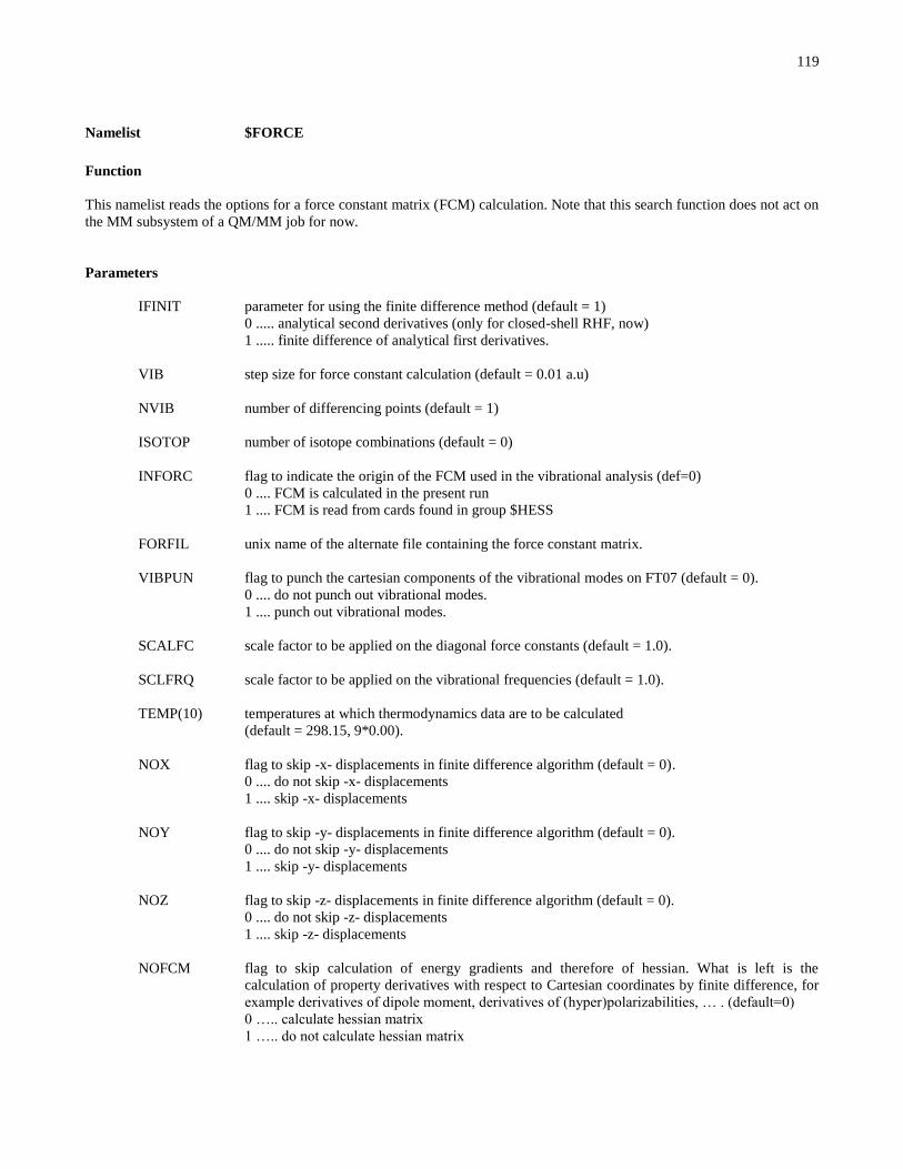
119

Namelist $FORCE

Function

This namelist reads the options for a force constant matrix (FCM) calculation. Note that this search function does not act on

the MM subsystem of a QM/MM job for now.

Parameters

IFINIT parameter for using the finite difference method (default = 1)

0 ..... analytical second derivatives (only for closed-shell RHF, now)

1 ..... finite difference of analytical first derivatives.

VIB step size for force constant calculation (default = 0.01 a.u)

NVIB number of differencing points (default = 1)

ISOTOP number of isotope combinations (default = 0)

INFORC flag to indicate the origin of the FCM used in the vibrational analysis (def=0)

0 .... FCM is calculated in the present run

1 .... FCM is read from cards found in group $HESS

FORFIL unix name of the alternate file containing the force constant matrix.

VIBPUN flag to punch the cartesian components of the vibrational modes on FT07 (default = 0).

0 .... do not punch out vibrational modes.

1 .... punch out vibrational modes.

SCALFC scale factor to be applied on the diagonal force constants (default = 1.0).

SCLFRQ scale factor to be applied on the vibrational frequencies (default = 1.0).

TEMP(10) temperatures at which thermodynamics data are to be calculated

(default = 298.15, 9*0.00).

NOX flag to skip -x- displacements in finite difference algorithm (default = 0).

0 .... do not skip -x- displacements

1 .... skip -x- displacements

NOY flag to skip -y- displacements in finite difference algorithm (default = 0).

0 .... do not skip -y- displacements

1 .... skip -y- displacements

NOZ flag to skip -z- displacements in finite difference algorithm (default = 0).

0 .... do not skip -z- displacements

1 .... skip -z- displacements

NOFCM flag to skip calculation of energy gradients and therefore of hessian. What is left is the

calculation of property derivatives with respect to Cartesian coordinates by finite difference, for

example derivatives of dipole moment, derivatives of (hyper)polarizabilities, … . (default=0)

0 ….. calculate hessian matrix

1 ….. do not calculate hessian matrix

120

IFQMMM flag to indicate whether the hessian calculation should include the MM subsystem or be limited

to the QM subsystem (default = 0)

0 …. hessian calculation restricted to the QM subsystem

1 …. hessian calculation includes the MM subsystem (not active yet)

Comments

In HONDO the second derivatives of the energy are most often calculated by finite difference of first derivatives. Infrared

and Raman intensities can be calculated by setting NOPROP = 0 in $CNTRL. By default the dipole moment and thus the

infrared intensities are calculated. To get the polarizabilities and thus the Raman intensities, NODPL must also be set equal

to 0 in $PRP.

This approach to the calculation of Raman intensities is likely to be time consuming, as one can gather from the comments

given about polarizability calculations (see $DPL). An alternative approach, with RUNFLG = 6 in $CNTRL, is proposed

below.

It is possible to calculate the dipole and polarizability derivatives using a different technique and without calculating the

force constant matrix. See $IRRAM for details. If this latter approach is used, then three runs are needed to get the

intensities:

calculate force constant matrix (RUNFLG = 2 in $CNTRL and INFORC = 0in $FORCE);

calculate dipole derivatives $MUD and polarizability derivatives $RAM (RUNFLG = 6 in $CNTRL and see $IRRAM);

calculate vibrational intensities using $MUD and $RAM (RUNFLG = 2 in $CNTRL and INFORC = 1 in $FORCE)

Analytical second derivatives may be calculated for closed-shell RHF wave functions only. In this case VIB and NVIB

parameters are ignored.

VIB is the step size for atomic displacement. The default seems to be adequate.

NVIB indicates whether a one or two point difference formula is used. A two-point difference formula gives a FCM that is

more accurate than when using a one point difference formula. The program is set up so that all the positive displacements

of the atoms are done first, then all the negative displacements. It is possible to first run a job with NVIB = 1, then to decide

that one really wants better accuracy, and run a restart job with NVIB = 2 without wasting any CPU time whatsoever. In

fact this is the approach that we recommend:

run initial job with NVIB = 1. and save the DA10 file .

change NVIB to NVIB = 2 in $FORCE, and set IREST = 1 in $CNTRL, and run job after attaching the DA10 file.

In some cases the additional accuracy of NVIB = 2 is not needed, so that one can go through the first step only. If at a later

time the user decides that the better accuracy is really what he wants, then by restarting the job as in step 3 described above,

he can still do so as long as the DA10 file was kept intact. Cost wise the two-point formula is twice as expensive as the one

point formula.

Finally note that if the molecule belongs to a symmetry point group (specified in $BASIS), only the unique atoms are

displaced in carrying out the finite difference algorithm, which can greatly reduce the CPU time.

ISOTOP is used to do isotope substitutions when calculating the vibrational frequencies and normal modes. A set of

standard masses is stored in the program, and a vibrational analysis with these is always carried out, followed by the isotope

substitutions. The default set up is such that only the standard isotope combination is used. The isotope combinations are

given in the data group $MASS. All the $MASS data groups must be stacked up one behind the other.

INFORC is used to perform a vibrational analysis when the force constant matrix is known and read from cards.

SCALF is a scale factor sometimes used to scale the diagonal force constants when expressed in the internal coordinate

basis. A scale factor of 0.9 is applied by some researchers. The default is to apply no scaling.

121

Namelist $MASS

Function

This namelist provides the atomic masses to be used in force constant, properties, and internal coordinates calculations.

Parameters

AMASS(128) Atomic masses of atoms (unique and non-unique) in the order generated by the

program to be used in vibrational analysis (default = standard average mass of common

isotopes)

Comments

The masses must be specified in the order in which the atoms appear in the run. This order is the same as the order at input

time ($BASIS) if no molecular symmetry is specified. If molecular symmetry has been specified in $BASIS the order of the

atoms is not straightforward but depends on the symmetry point group and on the molecule. Masses for the symmetry

equivalent atoms (these atoms were not given in $BASIS) must be specified here. If molecular symmetry was given in

$BASIS but the parameter NOSYM was set equal to 1 in $CNTRL, the order of the atoms is also somewhat disconcerting.

Basically NOSYM does not affect the input in the present namelist $MASS

Namelists $MASS must be stacked up one behind the others when several mass combinations are used.

For (hyper)polarizability calculations where the masses are just used to determine the center of mass and the inertial axes,

only the last namelist $MASS is used.

122

Namelist $HSSINP

Function

Parameters

NFRAG number of fragments used in constructing the hessian matrix of the system

(default = 1)

LFRAG(128) length (in terms of number of atoms) of fragments used in the constructions of the hessian

matrix of the system. The atoms that make up the fragments and the system must be in the same

order. The $HESS of the various fragments must be stacked one after the other.

Comments

123

Data group $HESS

Function

This input group contains a force constant matrix also called Hessian. It is used in conjunction with $OPT, $SAD, $IRC,

$FORCE. In fact it is generated by a run in which RUNFLG = 2 in $CNTRL

Cards

ICOORD, ICARD, H(ICOORD,5*(ICARD-1)+1), H(ICOORD,5*(ICARD-1)+2

FORMAT(I2,I3,5E15.8)

Each coordinate starts a new card. For larger molecules with more than 33 atoms (more than 100 coordinates) a

FORMAT(I3,I2,5E15.8) is used. The program automatically sets the correct format.

124

Namelist $IRRAM

Function

This namelist controls the calculation of dipole moment and polarizability derivatives with respect to Cartesian nuclear

coordinates. It is used when RUNFLG = 6 in $CNTRL. The program generates the data groups $MUD and $RAM for

subsequent use in a vibration analysis to obtain the derivatives with respect to the normal modes, quantities closely related

to infrared and Raman intensities. The method used is the one described by Komornicki and McIver, and is valid for any

SCF wave function, single determinantal or multiconfigurational. The reference is: A. Komornicki and J.W. McIver,Jr. ,

J.Chem.Phys. 70, 2014 (1979)

Parameters

FIELD strength of the uniform electric field acting on the molecule (default = 0.001).

NOINT flag to specify calculation of intensities from energy derivatives (default = 0).

0 ....... calculate intensities

1 ....... do not calculate intensities

NORAM do skip terms for Raman intensities

Comments

The namelist $IRRAM does not have to be present if the default value of FIELD is good enough. This program can be used

to get infrared and Raman intensities without calculating the dipole and polarizability at each perturbed point in the force

constant calculation.

One possible sequence of jobs is:

calculate the force constant matrix with RUNFLG = 2 in $CNTRL and save data group $HESS from the punch

file FT07

calculate dipole and polarizability derivatives with RUNFLG = 6 in $CNTRL and save the data groups $MUD and

$RAM from the punch file FT07 .

add $HESS , $MUD and $RAM to input data, set INFORC = 1 in $FORCE , and run with RUNFLG = 2 in

$CNTRL.

A second possible sequence is:

run with RUNFLG = 6 in $CNTRL , and save data groups $MUD and $RAM.

add $MUD and $RAM to input data and run with RUNFLG = 2, NOPROP = 1 in $CNTRL.

125

Data group $MUD

Function

This data group, generated by a run with RUNFLG=2, NOPROP = 0or RUNFLG = 6 in $CNTRL, contains the derivatives

of the dipole moment with respect to the nuclear coordinates. It can be used in a vibration analysis to get the infrared

intensities, if the force constant matrix is available. The first card contains the three components of the dipole moment. The

next card(s) contain(s) the 3*NUC derivatives of the -x- component of the dipole moment (where NUC is the number of

nuclei), then we have the derivatives of the -y- component, and finally the derivatives of the -z- component.

Cards

DMUX, DMUY, DMUZ

FORMAT(5X,3F15.8)

IXYZ, ICARD, DMU(1+5*(ICARD-1)), DMU(2+5*(ICARD-1)), ...

FORMAT(I2,I3,5F15.8)

IXYZ is the component number of the dipole moment (1, 2 or 3), ICARD if the card number for the derivatives.

There are 3*NUC derivatives, and five at the most are stored on a given card. All the derivatives of a given dipole

component are given together, for each component a new card is started.

Comments

The derivatives calculated in this run are intended to be used in conjunction with a force constant matrix to obtain the

vibrational intensities. See the comments for the namelists $FORCE and $IRRAM regarding the sequence of runs needed

for this purpose.

126

Data group $RAM

Function

This data group, generated by a run with RUNFLG = 6 in $CNTRL, contains the derivatives of the polarizability tensor

with respect to the nuclear coordinates. It can be used in a vibration analysis to get the Raman intensities, if the force

constant matrix is available The first card contains the six components of the polarizability tensor. The next card(s)

contain(s) the 3*NUC derivatives of the -XX- component of the tensor (NUC is the number of nuclei), then we have the

derivatives of the -YY- component, of the -ZZ- component, of the -XY- component, of the -XZ- component, and finally of

the -YZ- component.

Cards

ALPHXX,ALPHYY,ALPHZZ,ALPHXY,ALPHXZ,ALPHYZ

FORMAT(5X,3F15.8)

IXYZ,ICARD,DALPH(1+5*(ICARD-1)),DALPH(2+5*(ICARD-1)), ...


IXYZ is the component number of the polarizability tensor (1 to 6). ICARD if the card number for the derivatives.

There are 3*NUC derivatives, and five at the most are stored on a given card. All the derivatives of a given

polarizability component are given together, for each component a new card is started.

Comments

The derivatives calculated in this run are intended to be used in conjunction with a force constant matrix to obtain the

vibrational intensities. See the comments for the namelists $FORCE and $IRRAM regarding the sequence of runs needed

for this purpose.

127

Namelist $NLO

Function

This namelist defines the calculation of molecular polarizability α and hyperpolarizabilities β and γ by the finite field

approach. The algorithm applies to any wave function and energy, regardless of whether analytical derivatives exist or not.

This is to be contrasted to the $DPL , $FPL , ... namelists called in the property calculation (see $PRP) which apply to

closed shell SCF wave functions only. Here we can use any wave function.

The algorithm is an extension of the formulae proposed by Kurtz et al. (J.Comp.Chem. 11, 82 (1990)), and is described in

F.Sim et al. (J.Phys.Chem. 97, 1158 (1993)).

Parameters

NORDER order of fitting polynomial (default = 6).

NFIELD number of positive field values to be used in fitting (default = 3). An identical number of

negative field values are used as well. The default value corresponds to a total of 7 field values,

in accord with NORDER.

FIELD base field strength (default = (0.02/nfield)a.u.)

IFX to specify direction of the field (default = 1).

0 .... do not do field pointing along -x- direction

1 .... do field pointing along -x- direction

IFY to specify direction of the field (default = 1).

0 .... do not do field pointing along -y- direction

1 .... do field pointing along -y- direction

IFZ to specify direction of the field (default = 1).

0 .... do not do field pointing along -z- direction

1 .... do field pointing along -z- direction

IF2D to specify a two-dimensioanl fitting (default = 0)

0 …. 1D fitting

1 …. 2D fitting

IFXY to specify direction of the field (default = 1).

0 .... do not do field pointing along -xy- plan

1 .... do field pointing along –xy- plan

IFXZ to specify direction of the field (default = 1).

0 .... do not do field pointing along -xz- plan

1 .... do field pointing along –xz- plan

IFYZ to specify direction of the field (default = 1).

0 .... do not do field pointing along -yz- plan

1 .... do field pointing along –yz- plan

Comments

The default values are set so that the program loops over the -x- , -y- , and -z- directions. In 2D, the program loops over the

–xy- , -xz- , and –yz- planes, and calculates all possible elements resulting from 2D terms.

128

Namelist $DYN

Function

This namelist governs the Molecular Dynamics driver.

Parameters

IFOPT Flag to carry out energy minimization by means of the MD driver (steepest descent path,

temperature set to 0.5 K) (default = 0)

0 … finite temperature MD

1 … energy minimization

TOLOPT convergence criterion on largest component of Cartesian gradient when IFOPT=1

(default = 0.0008; same as in namelist $OPT)

TEMP temperature

(default = 298K)

TIMSTP time step

(default = 0.5 femtosecond)

NSTEP number of MD steps

NPTDYN same as NSTEP: number of MD steps

SEED seed for random generator for initial velocities

(default = 0.00)

NSAVE interval in units of STEP's for saving MD geometries (default = 10)

IPTSAV same as NSAVE

IREST (deault = 0)

NORMKE (default = 1)

IFVEL (default = 0)

IEQUIL flag to equilibrate by Monte Carlo algorithm the MM subsystem of a QM/MM system

(default = 1)

0 … do not equilibrate

1 … equilibrate

PERIOD (not active)

VERLET (not active)

Comments

129

Namelist $PES

Function

Given several geometries for which the energy and possibly the gradients with respect to the nuclear coordinates must be

calculated, the program loops over these geometries.

Parameters

NPES number of points on the potential surface that must be calculated. The geometries must be given

in the data groups $XYZ, which must be stacked one behind the others in the input file (default

= 1). When the LST option or the QST option is activated, NPES is the number of points that the

program generates on the LST path or the QST path. In these cases, only two and three points

need to be read in respectively, corresponding to the initial, intermediate (in the QST case), and

final points on the path.

IUNIT parameter to indicate the units in which the atomic coordinates of the points on the surface are

given. (default = -1)

-1 .... coordinates in atomic units

1 .... coordinates in angstroms

0 .... not allowed (corresponding to internal coordinates in $BASIS)

NOGRD parameter to indicate whether the energy gradients must also be calculated at each point (default

= 1; option presently inactive)

0 .... calculate gradients.

1 .... do not calculate gradients.

MODVEC parameter to indicate which orbitals to use as starting guess at each point (default = 0)

0 …. use converged orbitals from first point

1 …. use converged orbitals from previous point

NPUNCH parameter to punch out the molecular orbitals (default = 0)

0 …. punch out orbitals from the first point only

1 …. punch out orbitals at every point

LST flag to activate Linear Synchronous Transit option (default = 0)

0 …. do not activate LST

1 …. activate LST

QST flag to activate Quadratic Synchronous Transit option (default = 0)

0 …. do not activate QST

1 …. activate QST

Comments

When the LST option is activated only two $XYZ data sets are needed. The should be the first point and the last point on a

LST pathway. The intermediate points are automatically generated by the program by linearly combining the first point and

the last point. With the LST option on, MODVEC=1 is forced.

The QST option is similar to the LST option but a third point corresponding to an intermediate geometry is needed. The

data sets $XYZ correspond to the first point, the intermediate point, and the last point in that order. The rest of the points

are automatically generated by the program by quadratically combining the three given points. The number of points must

be odd (a point is added if the given NPES is even). MODVEC=1 is forced as well here.

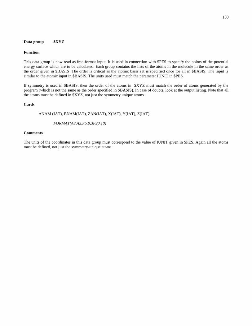
130

Data group $XYZ

Function

This data group is now read as free-format input. It is used in connection with $PES to specify the points of the potential

energy surface which are to be calculated. Each group contains the lists of the atoms in the molecule in the same order as

the order given in $BASIS .The order is critical as the atomic basis set is specified once for all in $BASIS. The input is

similar to the atomic input in $BASIS. The units used must match the parameter IUNIT in $PES.

If symmetry is used in $BASIS, then the order of the atoms in $XYZ must match the order of atoms generated by the

program (which is not the same as the order specified in $BASIS). In case of doubts, look at the output listing. Note that all

the atoms must be defined in $XYZ, not just the symmetry unique atoms.

Cards

ANAM (IAT), BNAM(IAT), ZAN(IAT), X(IAT), Y(IAT), Z(IAT)

FORMAT(A8,A2,F5.0,3F20.10)

Comments

The units of the coordinates in this data group must correspond to the value of IUNIT given in $PES. Again all the atoms

must be defined, not just the symmetry-unique atoms.

131

Namelist $TRUDGE

Function

This namelist requires the simultaneous definition of the namelist $GEXP. This namelist defines the parameter for a non-

gradient optimization of exponents or coordinates for example. The optimization is done by means of the TRUDGE

program (written by Prof. H.F. King at the University of Buffalo) based on conjugate gradient optimization search. The

optimization is defined by the routine EXPNRG that assigns the parameters to be optimized. The routine is presently set up

to optimize Gaussian exponents of uncontracted primitives, without enforcing any constraints (two non-symmetry

equivalent H atoms have their p function exponents optimized separately). The user may have to modify the source code in

this subroutine to tailor it to his own specification.

Parameters

KSTART indicates the conjugate gradient direction in which the optimization will proceed (default = -1)

-1 ....indicates that this is a non-restart run.

0 ....corresponds to a restart run.

TIMLIM maximum CPU time for the optimization to go on. The program times out then and punches on

FT07 all the restart data to be read in a subsequent run. These data include JSTART, TOLF,

TOLR, FNOISE, FNOT, RNOT, CURV, ALPH, and V. For further information, see the source

code in the file dr2.f (default = 100000.0 seconds).

Comments

There are more parameters in the namelist $TRUDGE, but those are concerned with restart capabilities. The code punches

the correct pieces of information on file FT07 in the form of a namelist! As a result the namelist maybe copied from the

FT07 file into the input file and the job can be restarted.

132

Namelist $GEXP

Function

This namelist defines parameters associated with the non-gradient optimization carried out with the EXPX driver, the input

of which is given in $TRUDGE . There is no general routine that has the flexibility to define every type of optimization.

The present scheme allows optimization of basis set exponent, without any constraints. A user can write his own version of

the routine EXPNRG to define his own optimization scheme. Presently the program allows for the optimization of 15

parameters.

Parameters

IEX(15) Defines the serial number of the Gaussian primitives for which the exponent must be optimized.

P(15) Defines the initial values of the exponents to be optimized.

133

Namelist $SEAM

Function

This namelist controls the search for a quasi-diabatic transition state, i.e. the minimum point energy on the crossing seam

surface between EA, the potential energy surface (PES) of the reactants, and EB, the PES of the products. The namelist

$SEAM is used when RUNFLG = 9 is selected in $CNTRL. A detailed description of the algorithm and a brief review of

the relevant concepts are given in: A. Farazdel and M. Dupuis,: J. Comput. Chem. 12, 276 (1990); A. Farazdel, M. Dupuis,

E. Clementi and A. Aviram, : J. Am. Chem. Soc. 112, 4206 (1990).

Parameters

CVGSM Convergence threshold on the largest component of the seam projection of the gradient vector of

EA or that of EB (default = 0.0005)

NPTSM Maximum number of Lagrangian function calculations (default = 50)

INHESS Input option for H(0)

, the initial hessian of the Lagrangian. (default =1)

0 .... set H(0)

to a predefined matrix.

1 .... Input H(0)

A. and H(0)

B.

2 .... Input H(0).

HSSFIL unix name of the alternate file containing the hessian matrix.

ICFRZ(384) Serial number of internal coordinates frozen in the search (default = 384*0)

CLAG0 The initial value of the Lagrange multiplier. (default = 0.5)

CEA, CEB Coefficients of EA and EB in the definition of the Lagrangian function.

(default = 0.5, 0.5)

NPFLG Print flag. (default = 0)

0 ..... standard output.

1 ..... intermediate debug printing.

2 ..... exhaustive debug printing.

MODUPD Update option. (default = 2)

1 ..... use BFGS update.

2 ..... use PSB update.

LINSM Not active yet.

Comments

To facilitate the convergence in this namelist, it is recommended to read in an initial hessian matrix, i.e. option INHESS = 1

or 2. The case INHESS = 1 can be achieved by running a force constant calculation ($FORCE) on the A state and the same

for the B state using a small basis set if preferred. The case INHESS = 2 can be used when there is a hessian already

available from a similar case. In addition, we recommend using an initial geometry which is in between the equilibrium

geometry of the A state and that of the B state. For more details see the first reference given at the beginning of this

namelist.

134

Namelist $ET

Function

This namelist specifies the parameters used in the calculation of intramolecular electron transfer properties (including the

ubiquitous VAB the electron-transfer matrix element) of molecules represented by the reaction 'A' arrow 'B' where A and

B denote two different charge-localized symmetry-broken (or simply localized) electronic states of the same molecule. A

localized wave function is not to be confused with the more common charge-delocalized symmetry-constrained (or simply

delocalized) wave functions. The namelist $ET is used when RUNFLG = 10 is selected in $CNTRL. In addition, you may

have to set parameters BSTATE and BETA in $GUESS and MOORDR in $SCF. For a description of the basic concepts

and the method used refer to: A. Farazdel and M. Dupuis, J. Comput. Chem. 12, 276 (1990); A. Farazdel, M. Dupuis, E.

Clementi and A. Aviram, J. Am. Chem. Soc. 112, 4206 (1990).

Parameters

MO1, MO2 Serial numbers of the two molecular orbitals being linearly combined or flipped. (default = 0, 0)

NOLC For the purpose of having a localized initial guess when the input is of a delocalized type, this

flag indicates whether the molecular orbitals MO1 and MO2 are to be linearly combined. MO1

and MO2 are replaced by (MO1 + MO2) / sqrt(2) and (MO1 - MO2) / sqrt(2) respectively

(default = 1)

0 ..... linearly combine

1 ..... skip

NOFLIP To make a second localized initial guess when only one is read in, this flag indicates whether

there is to be a flipping, i.e. exchanging MO1 with MO2 (default = 1)

0 ..... perform flipping

1 ..... skip

IVUOPT Flag to indicate which one of the two existing subroutines is to be used to carry out the

corresponding orbital transformation step (default = 0)

0 ..... use DSVDC

1 ..... use ETVRU

IETOUT Print flag. (default = 0)

0 ..... standard output

2 ..... intermediate debug printing

3 ..... exhaustive debug printing

ETA energy of A state (default = 0.0). Non-zero values of ETA and ETB make the program skip the

wave function and energy calculations for the quasi-diabatic states.

ETB energy of B state (default = 0.0). Non-zero values of ETA and ETB make the program skip the

wave function and energy calculations for the quasi-diabatic states.

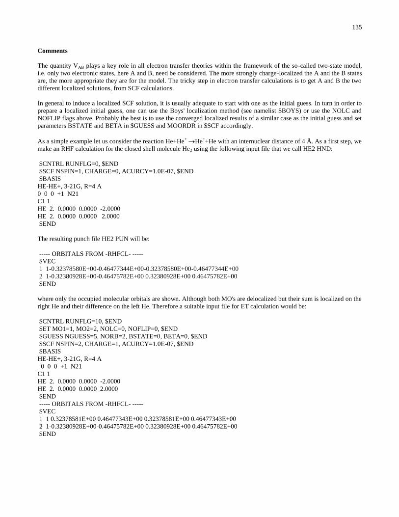
135

Comments

The quantity VAB plays a key role in all electron transfer theories within the framework of the so-called two-state model,

i.e. only two electronic states, here A and B, need be considered. The more strongly charge-localized the A and the B states

are, the more appropriate they are for the model. The tricky step in electron transfer calculations is to get A and B the two

different localized solutions, from SCF calculations.

In general to induce a localized SCF solution, it is usually adequate to start with one as the initial guess. In turn in order to

prepare a localized initial guess, one can use the Boys' localization method (see namelist $BOYS) or use the NOLC and

NOFLIP flags above. Probably the best is to use the converged localized results of a similar case as the initial guess and set

parameters BSTATE and BETA in $GUESS and MOORDR in $SCF accordingly.

As a simple example let us consider the reaction He+He+ He

++He with an internuclear distance of 4 Å. As a first step, we

make an RHF calculation for the closed shell molecule He2 using the following input file that we call HE2 HND:

$CNTRL RUNFLG=0, $END

$SCF NSPIN=1, CHARGE=0, ACURCY=1.0E-07, $END

$BASIS

HE-HE+, 3-21G, R=4 A

0 0 0 +1 N21

C1 1

HE 2. 0.0000 0.0000 -2.0000

HE 2. 0.0000 0.0000 2.0000

$END

The resulting punch file HE2 PUN will be:

----- ORBITALS FROM -RHFCL- -----

$VEC

1 1-0.32378580E+00-0.46477344E+00-0.32378580E+00-0.46477344E+00

2 1-0.32380928E+00-0.46475782E+00 0.32380928E+00 0.46475782E+00

$END

where only the occupied molecular orbitals are shown. Although both MO's are delocalized but their sum is localized on the

right He and their difference on the left He. Therefore a suitable input file for ET calculation would be:


$ET MO1=1, MO2=2, NOLC=0, NOFLIP=0, $END

$GUESS NGUESS=5, NORB=2, BSTATE=0, BETA=0, $END


$BASIS

HE-HE+, 3-21G, R=4 A

0 0 0 +1 N21

C1 1

HE 2. 0.0000 0.0000 -2.0000

HE 2. 0.0000 0.0000 2.0000

$END


$VEC

1 1 0.32378581E+00 0.46477343E+00 0.32378581E+00 0.46477343E+00

2 1-0.32380928E+00-0.46475782E+00 0.32380928E+00 0.46475782E+00

$END

136

with the following summary of results:

Total Energy = EA = EB = -4.8110620336 a.u.

SAB = <A||B> = -0.0006050204

HAB = <A | H | B> = 0.0032564385 a.u. where H is the total electronic hamiltonian.

VAB = 5.593 cm–1

= 0.016 kcal/mol.

Finally there is the question of geometry. At what geometry should one calculate VAB? Fortunately, according to the

Condon approximation the value of VAB is not very sensitive to the geometry as long as the distance between the donor to

the acceptor region in the molecule does not change significantly. More accurately, the geometry of the nuclear frame

should correspond to either an adiabatic transition state (see namelist $SAD) or a quasi-diabatic transition state (see

namelist $SEAM) depending upon the value of VAB. For more details refer to the references mentioned at the beginning of

this namelist.

137

Namelist $ZMAT , $ZMT

Function

This namelist controls the definition of the internal coordinates of the molecules. Note that the internal coordinates defined

in this namelist may or may not be the same as the one used to set up the molecular geometry in $BASIS. Symmetry

adapted coordinates can be specified by means of the arrays IJS and SIJ. These arrays can also be used to remove linear

dependencies among the internal coordinates. SIJ is basically a transformation matrix, usually sparse. Therefore only its

non-zero elements are inputted, via IJS. The entries in IJS are pairs of indices, a row index and a column index, defining the

non-zero elements of SIJ. Refer to the book: “Molecular Vibrations” by Wilson, Decius, and Cross, McGraw-Hill, New

York, 1955. Also see: P.Pulay, J.Am.Chem.Soc. 101,2554 (1979) for the question of linear dependencies.

Parameters

IZMAT(1800)

TYPE1,ATOM1,ATOM2

TYPE2,ATOM1,ATOM2,ATOM3

TYPE3,ATOM1,ATOM2,ATOM3,ATOM4

TYPE4,ATOM1,ATOM2,ATOM3,ATOM4

TYPE5,ATOM1,ATOM2,ATOM3,POINT

TYPE6,ATOM1,ATOM2,ATOM3,ATOM4,ATOM5

In this notation, TYPE specifies the type of internal coordinates. Possible types are:

TYPE = 1 for stretch: ATOM1 connected to ATOM2.

TYPE = 2 for bend: ATOM1 connected to ATOM2 connected to ATOM3.

TYPE = 3 for torsion: ATOM1 connected to ATOM2 connected to ATOM3 connected to

ATOM4.

TYPE = 4 for out of plane bend: ATOM1 connected to ATOM2 moves out of the plane of the

three other atoms, with ATOM2 connected to both ATOM3 and ATOM4.

TYPE = 5 for linear bend: ATOM1 connected to ATOM2 connected to ATOM3. POINT is an

additional point that defines a reference plane. Ten such points may be specified in A below.

POINT is the serial number of one of these addition points.

TYPE = 6 for angle between planes: ATOM1 connected to ATOM3 connected to ATOM2 form

a plane at an angle with the plane defined by ATOM4 connected to ATOM3 connected to

ATOM5.

IJS(2,750) pairs of indices for inputted symmetry coordinate coefficients given in SIJ.

SIJ(750) symmetry coordinate coefficients corresponding to index pairs given in IJS.

NZMOD number of symmetry or independent coordinates kept in the construction of the B matrix, or of

the modified B matrix. In general 3*NUC-6 (or 3*NUC-5) coordinates should be kept, where

NUC is the number of nuclei. Sometimes it is advantageous to keep fewer (frozen coordinates in

an optimization) or more (determination of dependent coordinates) (default = 0)

0 ..... keep 3*NUC-6 (or 3*NUC-5) coordinates.

n ..... keep NZMOD = n coordinates.

138

A(3,10) Cartesian coordinates of points used to specify linear bends. For a given linear bend the point

corresponds to the fourth entry in IZMAT (default = 30*0.0E+00)

LINEAR indicates whether the molecule is linear or not (default = 0). This parameter has nothing to do

with the parameter of the same name in $BASIS . It is used to define the number of internal

coordinates.

0 ..... non-linear molecule

1 ..... linear molecule

Comments

Let us take CH2 as an example: assume the order of the atoms to be C , H , and H. The namelist would look like this:

$ZMAT

IZMAT=1,1,2, 1,1,3, 2,2,1,3,

$END

The first three digits defining IZMAT describe one CH stretch, the second set of three digits describes the other CH stretch,

the last four digits specify the HCH angle bend, for a total of three internal coordinates. If we now want to specify the

symmetrized internal coordinates, the namelist will look like this:

$ZMAT

IZMAT=1,1,2, 1,1,3, 2,2,1,3,

IJS=1,1, 2,1, 1,2, 2,2, 3,3,

SIJ=1.0, 1.0, 1.0,-1.0, 1.0,

$END

IJS and SIJ specify the symmetry matrix to define the symmetric stretch, the antisymmetric stretch, and the bend. This is a

3 by 3 matrix. The pairs of digits IJS tell us that the elements 1,1, 2,1, 1,2, 2,2, and 3,3, have the values given by SIJ. The

symmetrization matrix is therefore:

1.0 1.0 0.0

1.0 -1.0 0.0

0.0 0.0 1.0

The program normalizes the columns of the matrix. Similarly these IJS and SIJ can be used to define linearly independent

(symmetrized) internal coordinates. A good reference regarding this question is: P. Pulay, J.Am.Chem.Soc. 101, 2554

(1979).

Take HCN as another example: assume that the atoms are in the order H, C, and N aligned along the x-axis. The namelist

ought to look like this:

$ZMAT

IZMAT=1,1,2, 1,2,3, 5,1,2,3,1,

A=1.0, 1.0, 0.0,

LINEAR=1,

$END

We recognize the meaning of the first two sets of three digits defined as IZMAT. They are the two stretches HC and CN.

The next five digits define a linear bend (type 5) that involves atoms 1, 2, and 3. Let us suppose that these three atoms are

on the X-axis. To define the two degenerate components of the bend, we must define a reference plane, by means of the

very last entry in IZMAT, in this case 1. This 1 tells us to look at the first point defined by the three entries of A. This point

happens to be the diagonal point in the XY-plane, and combined with the atoms H and N defines the XY plane as the

reference plane. Note that the A point could have been anywhere in the XY-plane to define this same plane as a reference.

The only requirement is that it not be collinear with the molecular axis. Note that a linear bend defines two bending modes

and thus we have indeed four internal coordinates, as we ought to.

139

Take HCCH as another example to show off this linear bend: the namelist ought to look like this:

$ZMAT

IZMAT=1,1,2, 1,2,3, 1,3,4, 5,1,2,3,1, 5,2,3,4,2,

A=0.0, 1.0, 0.0, 0.0, 0.0, 1.0,

LINEAR=1,

$END

In this example there are two linear bends to be defined, one for HCC and the other for CCH. In our example we chose to

use two different reference planes for the two linear bends. Note that we have defined here a total of seven internal

coordinates.

140

Namelist $GUESS

Function

This namelist defines the parameters necessary to generate an initial guess for a SCF or MCSCF calculation or to read in

the orbitals in a CI, MCSCF, or properties calculation.

Parameters

NGUESS initial orbital guess option (default = 2)

1 .... not active

2 .... bare nucleus Hamiltonian orbitals

3 .... Huckel guess for basis sets based on the STO-nG bases

4 .... Huckel guess for basis sets based on the N-31G or N-21G bases

5 .... orbitals read from cards

6 .... orbitals read from DA10

7 .... Huckel guess for basis sets based on the DZV bases

8 .... concatenation of fragment orbital sets

NORB Number of orbitals to be read in when NGUESS = 5 .

Also number of orbitals to be printed.

NFORMT flag to set the format for reading the input orbitals when NGUESS = 5

(default = 0)

0 .... FORMAT(I2,I3,5E15.8)

1 .... FORMAT(I2,I3,15F5.2)

NORDER flag to reorder the orbitals (default = 0)

0 .... do not reorder the orbitals

1 .... reorder the orbitals; new order specified with IORDER

IORDER new order of the orbitals if NORDER = 1. This is an array of dimension 3072 .

(default = canonical order 1,2,3,...NORB)

IORDRA new order of α spin orbitals for UHF calculation. This is an array of

dimension 3072.


IORDRB new order of β spin orbitals for UHF calculation. This is an array of

dimension 3072.


MORDER flag to reorder the basis functions of the initial guess orbitals (default = 0).

0 .... do not reorder the basis functions

1 .... reorder the basis functions; new order specified with JORDER

JORDER mapping of nuclei to old order, when MORDER = 1. This is an array of dimension 128

(default = canonical order 1,2,3,...NATOMS)

NFRAG number of fragment orbital sets used to build the initial guess set.

Only when NGUESS=8. (default = 1)

LFRAG(2,128) fragment orbital set data. This is an array of dimension 2*128 .

LFRAG(1,IFRAG) size of basis set for fragment IFRAG.

141

LFRAG(2,IFRAG) number of orbitals extracted from fragment IFRAG.

BETA flag to read in β spin orbitals in UHF runs (default = 0)

0 .... read only α spin orbitals

1 .... read both α and β spin orbitals

BSTATE flag to read in orbitals for a B-state (for RUNFLG = 9 or 10 in $CNTRL)

(default = 0)

0 .... read orbitals for one state only

1 .... read orbitals for two states

ZERTOL truncation threshold for the MO coefficients. The coefficients are truncated

beyond the decimal place which contributes less than ZERTOL to the coefficients. This

is useful to restore symmetry in nearly degenerate orbitals

for example by using a somewhat large value of ZERTOL. If ZERTOL = 0.0 ,

no truncation is performed. (default = 0.0)

NPUNCH flag to punch out the initial guess orbitals on file FT07. (default = 0)

0 .... do not punch orbitals

1 .... punch orbitals

NPFLG print flag (default = 0)

0 .... normal printing

1 .... debug printing

GSSFIL unix name of an alternate file containing the initial vectors.

PRTTOL threshold for printing vector coefficients (default = 0.2)

NROT flag to apply 22 rotations to orbitals (default = 0)

MOROT(2,64) pair of indices for orbital pair-wise rotations

MOROTA(2,64) pair of indices for orbital pair-wise rotations for orbitals

MOROTB(2,64) pair of indices for orbital pair-wise rotations for orbitals

Comments

When using NGUESS=5, the orbitals to be read in must be included in the input file under one of the data groups $VEC; or

$VECA, $VECB; and/or $VECA-A; $VECB-A, $VECA-B, $VECB-B (see below).

NGUESS = 3 or 4 will set up a Huckel Hamiltonian. The original routines from GAUSSIAN70 have been extended by

M.S. Gordon (University of North Dakota) to allow more flexibility. One may use NGUESS = 3 for basis sets based on the

STO sets. Diffuse and polarization functions are permitted in addition to the minimal basis set. Similarly, for the extended

initial guess routine that was created for the 4-31G , 5-31G , and 6-31G basis sets, diffuse and polarization functions are

permitted in addition to these double zeta valence sets.

Basis sets based on the N-21G sets with N = 3 or 6 can be handled with the NGUESS=4 option as well since they have the

same structure as the N-31G sets. Similarly NGUESS=7 may be used for basis sets based on the DZV sets of Dunning,

possibly extended with polarization and diffuse functions. For all other basis sets, use either NGUESS=2 or preferably

NGUESS=5 if possible.

The NORDER parameter along with IORDER (or IORDRA and IORDRB) is very useful and handy. It allows reordering

of the orbitals without much difficulty, a step often needed for MCSCF and CI calculations. Note that when NGUESS=6,

142

an option set up automatically for a restart job (IREST=1) for example, the reordering of the orbitals is not carried out, even

if requested (reordering orbitals that are in the correct order yields an incorrect starting set!).

Sometimes it is advantageous to make up an orbital set from fragment orbital sets. The option NGUESS = 8does just that.

This would be specially applicable to molecules that are composed of non-covalently bound fragments. NFRAG is the

number of fragments used in the partitioning of the molecule, and for each fragment IFRAG, LFRAG(1,IFRAG) and

LFRAG(2,IFRAG) are the basis set size for the fragment basis, and the number of orbitals extracted from the fragment. The

fragments must be ordered so as to make the correct molecule as a whole. The sum of the fragment basis set sizes must be

equal to the total number of basis functions. The sum of the number of fragment orbitals must be equal to the number of

orbital requested NORB. The fragment orbitals are given in as many data groups $VEC as there are fragments (NFRAG).

The $VEC data groups are stacked in the input data in the correct order one after the order ones. As an example, consider a

water dimer with a double-zeta basis set (50 basis functions). First one would run two jobs, one for each of the water

molecules, creating two $VEC data groups of 25 orbitals expressed in terms of the 25 basis functions. These two data

groups get stacked in the dimer input, and one would use:

$GUESS NGUESS=8, NORB=10, NFRAG=2, LFRAG=25,5, 25,5, $END

This input indicates that 10 dimer orbitals are created from 5 orbitals of the first water molecule (with 25 basis functions)

and 5 orbitals of the second water molecule (also with 25 basis functions). Note that the requirements 25 + 25 = 50 and 5 +

5 = 10 are satisfied.

The BETA = 1 option indicates that an α set of vectors in addition to a β set of vectors are to be read in via data groups

$VECA and $VECB.

The BSTATE = 1 option is used if initial guess vectors for two states (A and B) are to be read in. This is done with data

groups $VECA-A and $VECA-B. If in addition, the two states are described with UHF wave functions, then the data

groups $VECA-A, $VECB-A, $VECA-B, and $VECB-B are used.

The GSSFIL parameter corresponds to the aix file name of the file from which the initial vectors will be read. For example,

if the HONDO input file name.hnd contains the following input data :

$GUESS NGUESS=5, NORB=5, GSSFIL='name.vec', $END

then the data group $VEC with the five initial orbitals, will be read from the file name.vec which must reside on the disk.

143

Data group $VEC

Function

Orbital coefficients read in a fixed format. The format depends on the choice made with the NFORMT variable in

$GUESS.

Cards

IORB,ICARD,C(5*(ICARD-1)+1,IORB),C(5*(ICARD-1)+2,IORB),...

NFORMT = 0and the number of basis functions is less than 100:


NFORMT = 0and the number of basis functions is greater than 99:


NFORMT = 1and the number of basis functions is less than 100:


NFORMT = 1and the number of basis functions is greater than 99:


Comments

The orbitals are stored in the following manner: for a given orbital all coefficients are printed with 5 or 15 coefficients per

card. For each orbital there are most likely several cards. Thus each card contains three pieces of information: the orbital

number, the card number for that orbital, and up to five or fifteen coefficients. Each orbital starts on a new card.

Note that if the number of basis functions is greater than 99, then the program automatically switches to the appropriate

format FORMAT(I3,I2,5E15.8) for NFORMT = 0 or FORMAT(I3,I2,15F5.2) for NFORMT = 1. The user does not need to

handle these cases in any special way.

144

Data groups $VECA, $VECB

Function

Similar to $VEC but for a UHF calculation in which one wants to input both the and the vectors (BETA = 1 in

$GUESS). The data group $VECA is for the vectors and $VECB for the vectors.

145

Data groups $VECA-A, $VECB-A, $VECA-B, $VECB-B

Function

Similar to $VEC but for seam finding (namelist $SEAM) or electron transfer (namelist $ET) calculations where localized A

and B states are to be read in. The data group $VECA-A is for the vectors of the A state, $VECB-A for the vectors of

the A state, $VECA-B for the vectors of the B state, and $VECB-B for the vectors of the B state.

146

Namelist $INTGRL

Function

This namelist controls the computation of the two electron integrals (TEI) and their output format. The desirable situation is

that the executable module will have been constructed with the rysq.f file which contains quadruple precision routines for

the calculation of the Rys roots and weights of the numerical quadrature when nroot > 5. If quadruple precision is not

supported by the hardware, then rysd.f is been used, and this leads to numerical inaccuracies that affects calculations with

basis set with f and g functions only, and only when highly accurate integrals are needed. The user needs to be aware.

Parameters

INTSKP flag to skip the calculation of TEI (default = 0)

0 ..... calculate TEI

1 ..... skip calculation of TEI (they ought to be already on disk).

INTBUF TEI buffer size (default = 4096)

NPKFIL flag to indicate whether the P supermatrix will be constructed (default = 1)

0 ..... P supermatrix will be constructed.

1 ..... P supermatrix will not be constructed.

NKFIL flag to indicate whether the K supermatrix will be constructed (default = 1)

0 ..... K supermatrix will be constructed.

1 ..... K supermatrix will not be constructed.

LABFIL flag to indicate which label-packing format is to be used (default = 0)

0 ..... format is defined by default in routine HNDCTL

2 ..... use a 2-index label containing (ij) and (kl)

4 ..... use a 4-index label containing i , j , k , l

NHONDO flag to indicate whether Pople's integral computation technique may be used

(default = 0)

0 ... POPLE is used for s and p integrals and HONDO technique for d integrals.

1 ... HONDO technique only is used.

CUTOFF threshold for keeping the TEI on the integral file (default = 1.0E-09)

THIME cost factor for storing the TEI on disk in a semi-direct calculation (default = 5)

THIZE size factor for storing the TEI on disk in a semi-direct calculation (default = 1.0E-04)

MBYTES disk space size in M-bytes for storing the TEI on disk in a semi-direct calculation.

(default = no limits)

INTPCK flag to indicate whether the integral file is in compressed form (default = 0)

(option inactive)

0 ...... integral file is not in compressed form.

1 ...... integral file in compressed form.

NREC number of the last integral records already written on integral file. This is needed for restarting

in the middle of the integral computation step (default = 1)

INTLOC location of last integral in the NREC record of the integral file. This is needed for restarting in

the middle of the integral computation step (default = 1)

147

IST,JST,KST,LST

These parameters are the serial numbers of the starting shells in the integral computation step.

These four parameters are needed for restarting in the middle of the integral computation step

(default = 1,1,1,1).




Comments

Our experience is that the use of supermatrices for SCF calculations reduce the CPU time by about a factor of 2, although

the P-supermatrix file is larger than the file that would contain the normal TEI. If present the K-supermatrix file has the

same length as the P-supermatrix file. So overall the use of supermatrices increases the I/O activity somewhat for P-

supermatrices , and significantly for the P- and K-supermatrices. Note that the supermatrices are created on the fly with

almost no CPU overhead. When using the direct approach to RHF and UHF calculations, one must be concerned with

numerical accuracies. For single-point calculation the program uses the default values of CUTOFF (e.g. 1.0E-09) and the

corresponding ITOL. This is sufficient for SCF energies and properties, whose values match the standard values up to 1.0E-

07. For calculations that require the gradient of the direct SCF energy, a tighter threshold of CUTOFF is used (e.g. 1.0E-11)

which provides greater numerical stability.

Alternately one can use a semi-direct approach, in which all the integrals with cost factor greater than THIME are stored on

disk while all others are recomputed as needed. This approach requires some disk space, more than the full direct approach

but less than the conventional approach; it requires more CPU time than the conventional approach, but less than the full

direct approach. The other parameters used in this context are THIZE and MBYTES. Integrals whose magnitudes are

estimated to be less than THIZE are never stored on disk. A positive value of MBYTES give the number of mega-bytes of

storage reserved for the TEI. Once that amount of disk space is used, then the program proceeds in semi-direct mode. See

the comments regarding DIRECT in $CNTRL.

148

Namelist $WFN

Function

This namelist controls the type of wave function calculated.

Parameters

WFNFLG flag indicating the type of wave function (default = 0)

-1 ..... no wave function calculation

0 ..... RHF, UHF, GVB wave function calculation

1 ..... MCSCF wave function calculation

2 ..... GUGA-CI wave function calculation

3 ..... MRD-CI wave function calculation

4 ..... not active

5 ..... RHF / UHF + MP2 energy calculation

6 ..... RHF + MP4(SDTQ) energy calculation

7 ..... SCF + GUGA-CI

8 ..... SCF + MRD-CI

9 ..... MCSCF + MRD-CI

10 ..... CAS-SCF + MP2

11 …. MP2 only part of CAS-MP2

12 …. CAS-SCF + QDPT2

13 …. QDPT2 only part of CAS-QDPT2

14 …. RHF + CCSD (not active yet)

15 ..... CAS-SCF + Diabatization with CASSCF DMOs

16 ..... CAS-QDPT + Diabatization with MC-QDPT DMOs

17 ..... CAS-QDPT + Diabatization with CASSCF DMOs

Comments

In the introduction we commented on the availability of the modules that comprise the MRDCI program. After obtaining

explicit permission from Prof. B. Buenker and/or Prof. S. Peyrimhoff to obtain and use these modules, interested users may

contact us to obtain the modules.

Direct SCF calculations are available for closed shell RHF, open shell UHF wave functions, and CASSCF and MCSCF

wave functions, as well as for MP2 energy calculations (DIRECT = 1 in $CNTRL). Presently no Direct CI is available.

Diabatization is performed when WFNFLG is 15, 16, or 17, and this is supported in only HONDOPLUS.

149

Namelist $SCF

Function

This namelist controls the calculation of SCF wave functions. Closed shell (RHF) and open shell (ROHF) restricted HF

energies can be calculated, as well as GVB(PP) energies. Spin unrestricted (UHF) wave function energies can also be

determined. Closed shell calculation are done in the RHFCL routine. Spin unrestricted are done in the UHFOP routine.

Davidson's method , programmed for high spin cases only, is executed in RHFOP. More general single determinant wave

functions must use the GVB routine ROGVB that is also used for GVB calculations in the perfect pairing approximation.

Parameters

NCO number of closed shell in SCF calculation.

NSETO number of sets of open shells in SCF calculation.

NO(10) number of open shells in each set.

NPAIR number of GVB pairs in SCF calculation.

NSPIN spin multiplicity of the wave function (default = 1).

CHARGE total electronic charge (default = 0).

F coupling coefficients when GVBFLG = 1.

ALPHA A coupling coefficients when GVBFLG = 1.

BETA B coupling coefficients when GVBFLG = 1.

CICOEF CI coefficients when GVBFLG = 1.

RHFFLG flag to indicate whether the RHF method is used (default =0)

0 ...... do not use RHF

1 ...... use RHF

UHFFLG flag to indicate whether the UHF method is used (default =0)

0 ...... do not use UHF

1 ...... use UHF

GVBFLG flag to indicate whether the GVB method is used (default = 0)

0 ...... do not use the GVB program.

1 ...... use the GVB program.

DFTFLG flag to carry out a DFT / UDFT calculation (default = 0)

0 ….. Hartree-Fock SCF / UHF calculation

1 ….. DFT / UDFT calculation

DFTFUN flag to select DFT functional when DFTFLG=1 (default = 0)

1 ….. 'exact' Hartree-Fock exchange

2 ….. LDA

3 ….. BECKE88

4 ….. SLYP

5 ….. BLYP

6 ….. B3LYP

150

7 …... BPW91

8 …... MPW1K

9 …... mPW1PW91

1XXX …… BXLYP

Becke exchange functional and LYP correlation functional. The fraction of HF

exchange is user-defined by a three digit number in the following way:

Fraction HF exchange = XXX/1000, fraction of DFT exchange= 1 –

(XXX/1000).

Example: For a fraction of HF exchange of 0.5 with the Becke exchange

functional and the LYP correlation functional, the user would define

DFTUN=1500.

2XXX …… BXPW91

Becke exchange functional and PW91 correlation functional. The fraction of

HF exchange = XXX/1000.

Example: For a fraction of HF exchange of 0.001 with the Becke exchange

density functional and the PW91 correlation functional, the user would define

DFTFUN=2001.

3XXX…… MPWX

mPW exchange density functional and PW91 correlation functional. The

fraction of HF exchange = XXX/1000.

Example: For a fraction of HF exchange of 0.606 with the mPW exchange

functional and the PW91 correlation functional, the user would define

DFTUN=3606.

DAMP damping factor used in Davidson's damping method (default = 1.01)

DAMP0 minimum damping in Davidson's method (default = 0.0)

IEXTRP extrapolation interval in Davidson's damping method (default = 5)

VSHIFT value of orbital energy shift for virtual orbitals (default = 0.0).

OSHIFT value of orbital energy shift for open shell orbitals (default = 0.0).

ACURCY convergence criterion (default = 1.0E-05)

for closed shell SCF, criterion applies to density matrix

for open shell SCF, criterion applies to density matrix

for ROHF, and GVB SCF, criterion applies to SQCDF

for UHF SCF, criterion applies to density matrix

NOSLZ flag to disable the use of 'sleazy' cutoffs in the direct SCF algorithms. (default = 0)

0 ..... use sleazy cutoffs when starting direct SCF

1 ..... do not use sleazy cutoffs.

MAXIT maximum number of iterations (default = 30)

MICIT number of micro iterations in Davidson's open shell algorithm (default = 15)

NPUNCH flag to punch out molecular orbitals (default = 0)

0 ...... punch out orbitals.

1 ...... do not punch out orbitals.

MOPRT number of molecular orbitals printed and punched at the end of the SCF process

(default = number of canonical orthonormal orbitals, most often the number of basis functions).

151




MOORDR flag for selection method of the new orbitals during SCF (default = 0)

0 .... select based on the Aufbau principle

1 .... select based on the maximum overlap criterion with initial orbitals

Comments

The first group of parameters deal with the definition of the SCF wave function. Defaults are set for closed-shell RHF

calculations and UHF open-shell calculations. RHFFLG, UHFFLG, and GVBFLG are used to overwrite defaults.

The key point to remember when defining an open-shell configuration is that two half occupied shells whose spins are

coupled to form a triplet, belong to the same set of open-shells. NCO , NSETO , NO , NPAIR , and NSPIN define the

structure of the SCF configuration or of the GVB wave function when NPAIR is not equal to 0 . For wave functions other

than closed shell , the open shell orbitals or the valence bond orbitals are determined from several Fock operators. For an

open shell single determinantal wave function , the open shell orbitals are grouped by sets (there are NSETO of these) and

each set corresponds to a different Fock operator. Each set comprises one or more open shells , and this is specified by the

variable NO .

As an example , consider a triplet state with two electrons outside the closed shells (CH2(3B1); the input should be:

$SCF NCO=3, NSETO=1, NO=2, NSPIN=3, RHFFLG=1, $END

Alternately, and in many cases more simply, the wave function can be defined with CHARGE and NSPIN only. Thus we

could have used:

$SCF CHARGE=0, NSPIN=3, RHFFLG=1, $END

The above wave function may be determined using the method developed by Davidson, and indeed the program of this

method will be used since the wave function corresponds to a high spin case. For a open shell singlet CH2(1B1), the input

would look like this:

$SCF NCO=3, NSETO=2, NO=1,1, NSPIN=1, GVBFLG=1, $END

Each open shell orbital is obtained from its own Fock operator. In principle Davidson's algorithm could be used in this case

too, but in practice the code found in HONDO is not programmed for cases other than high spin. This is the reason why the

input data indicates that the GVB program will be used. The GVB program of course is designed to calculate GVB wave

functions, which are special forms of multiconfiguration wave functions. The energy expression that is minimized

corresponds to the expression for a general single determinantal wave function, and therefore the GVB program can be

used for the present purpose. The coupling coefficients F, ALPHA, BETA which define the energy expression are

internally stored for a few specific cases such as high spin cases and singlet open shells.

A warning is in order here: with the GVB code the following input streams ought to be equivalent:

$SCF NCO=3, NSETO=1, NO=2, NSPIN=3, GVBFLG=1, $END

$SCF NCO=3, NSETO=2, NO=1,1, NSPIN=3, GVBFLG=1, $END

For reasons that are not well understood yet, the former input does not seem to work, only the latter gives the correct result.

There appears to be a need to have only one and only one open shell defined by each Fock operator.

The same energy expression arises for average energies in the case of spatially degenerate states. It is then possible to use

the GVB program to calculate spin and spatial symmetry restricted wave functions such as the one for atomic states, or

152

open shell states of linear molecules . Good references for all these definitions are: C.C.J. Roothaan, Rev. Mod. Phys. 23,

69 (1951); E.R. Davidson, Chem. Phys. Lett. 21, 565 (1973); C.F. Jackels, and E.R. Davidson, Intern.J.Quant.Chem. 7, 707

(1974); F.W. Bobrowicz, and W.A. Goddard III, in Modern Theoretical Chemistry, Plenum, New York, 1977.

Note that in the case of GVB wave function calculations, the order of the occupied molecular orbitals is critical: closed

shells, open shells, GVB pair 1 orbital 1, GVB pair 1 orbital 2, GVB pair 2 orbital 1, GVB pair 2 orbital 2, ... . The orbitals

must be in this order at the beginning of the SCF process, and this may require that the orbitals be reordered during the

initial guess step (see $GUESS).

When using the ECP approximation, the core orbitals included in the core potential must not counted among the core

orbitals in the calculation. Sample 8 gives the input for a calculation on the formic acid molecule HCOOH in which an ECP

is used for C and O. With a 'normal' basis set, we would set NCO = 12. But since the three pairs of 1s electrons are included

in the ECP, the correct input in the namelist $SCF is NCO = 9.

There are several tools used to help the convergence of the various SCF programs. Extrapolation, damping, and level shift

are available. By default extrapolation is turned on and cannot be turned off, except by turning on damping or level shift.

Extrapolation works well toward the end of the SCF calculation. The extrapolation method is Pople's original algorithm for

restricted open-shell and GVB wave functions. For closed-shell and unrestricted open-shell wave functions, the

extrapolation method is Pulay's DIIS. Early on it is preferable to turn on damping or level shift.

When level shift is turned on by specifying VSHIFT and OSHIFT, it stays on always. It is intended that the calculation will

actually proceed in two jobs. Hopefully after a few iterations the SCF process is stabilized and the other methods of

convergence can be used. VSHIFT defines the shift of the virtual orbitals, and OSHIFT the shift of the open shell orbitals.

In practice we tend not to use the technique of level shift. It is our last recourse when other things have failed. We found

level shift most useful when dealing with transition metals. For most other cases damping combined with extrapolation

works well. When both level shift and damping are turned on with nonzero values of VSHIFT and DAMP, level shift takes

precedence.

To turn on damping, specify a nonzero value of DAMP. The damping scheme implemented corresponds to the following

equation:

D+1 = (D0 + DAMP * D-1) / (1.0 + DAMP)

The program uses an empirical algorithm developed by E.R. Davidson according to which the damping factor is adjusted

depending on the behavior observed during the SCF process. The algorithm has proven very powerful , and for just about

any closed shell molecule containing first and second row atoms , even using polarized basis sets , the program will

converge using the bare nucleus hamiltonian vectors as starting guess (NGUESS = 2 in $GUESS). The method seems to

work well even for UHF wave functions. Beyond these it is a good idea to generate good initial vectors for open shell

systems by carrying out calculations of UHF type or by calculating an ionic state.

With the availability of the DIIS algorithm for closed-shell and spin-unrestricted open-shell wave functions, the defaults

have been set so that damping kicks on only if DAMP is greater than some value DMPTOL = 1.0. For restricted open-shell

and GVB cases DMPTOL = 0.2. Combined with the default value of DAMP = 0.25, damping will not kick on for closed-

shell and unrestricted open-shell, unless DAMP is over-written, while damping will kick on for restricted open-shell and

GVB cases.

In practice we find that the convergence threshold ACURCY = 1.0E-05 works well for closed shell and UHF wave

functions. A tighter threshold ought to be used when properties such as force constants or (hyper)polarizabilities are

requested , as these depend on the actual SCF wave functions, and therefore a tighter convergence may be necessary. For

ROHF (Davidson's algorithm) or GVB calculations ACURCY = 1.0E-04 appears to be sufficient.

MAXIT controls the maximum number of iterations of the SCF process. When MAXIT = 0 , then the code computes the

energy from the initial orbitals, but does not perform any iteration. In the process the program has a genuinely correct

density matrix that can then be used to calculate properties. When MAXIT = -1, then the code does not even get into the

SCF program, and there is no correct density matrix built from the initial orbitals. This option is used only when restarting a

polarizability job, which requires unaltered (not even re-normalized) orbitals.

153

By defaults the direct SCF algorithms for closed-shell and UHF calculations use variable cutoffs. The program starts with

loose ('sleazy', 1.0e-06) cutoffs in the first few iterations when the density matrix is not very good, supposedly, so as to

reduce the number of electron repulsion integrals that need be computed. As convergence is coming, the program

automatically decreases the cutoffs down to their 'normal' values, so that at the end the energy has the accuracy we are

accustomed to.

However if the initial molecular orbitals (or equivalently density matrix) are very good, the inaccuracies from the 'sleazy'

cutoffs can be very damaging to the convergence process that may then take many more iterations than it would if we had

used tight thresholds in the first place. To force the program to use tight thresholds from the beginning, use NOSLZ = 1.

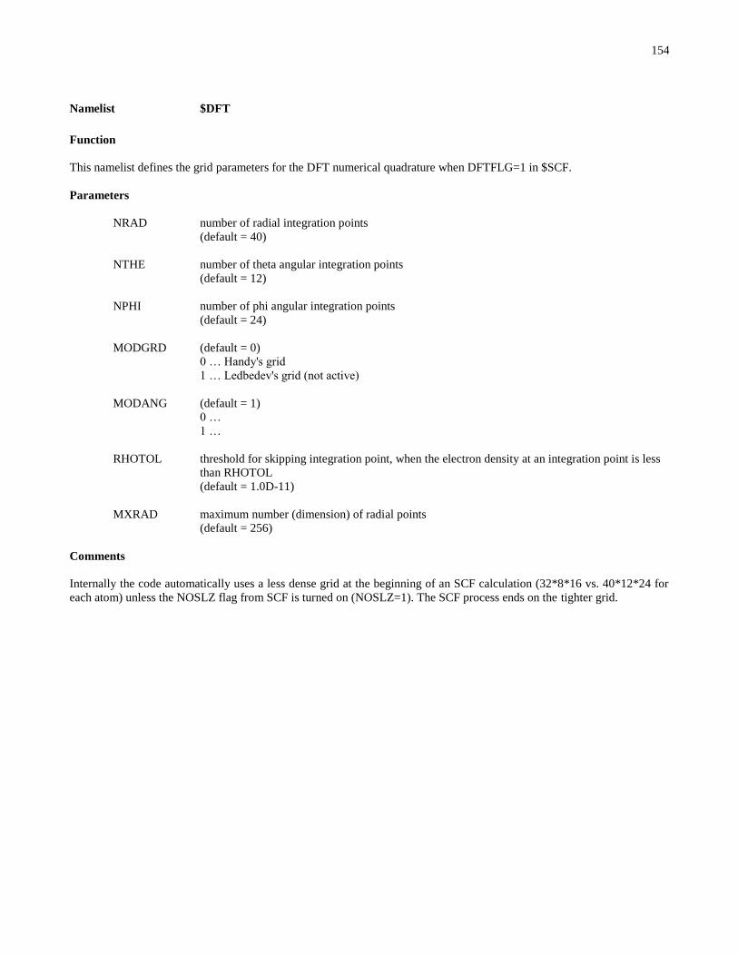
154

Namelist $DFT

Function

This namelist defines the grid parameters for the DFT numerical quadrature when DFTFLG=1 in $SCF.

Parameters

NRAD number of radial integration points

(default = 40)

NTHE number of theta angular integration points

(default = 12)

NPHI number of phi angular integration points

(default = 24)

MODGRD (default = 0)

0 … Handy's grid

1 … Ledbedev's grid (not active)

MODANG (default = 1)

0 …

1 …

RHOTOL threshold for skipping integration point, when the electron density at an integration point is less

than RHOTOL

(default = 1.0D-11)

MXRAD maximum number (dimension) of radial points

(default = 256)

Comments

Internally the code automatically uses a less dense grid at the beginning of an SCF calculation (32*8*16 vs. 40*12*24 for

each atom) unless the NOSLZ flag from SCF is turned on (NOSLZ=1). The SCF process ends on the tighter grid.

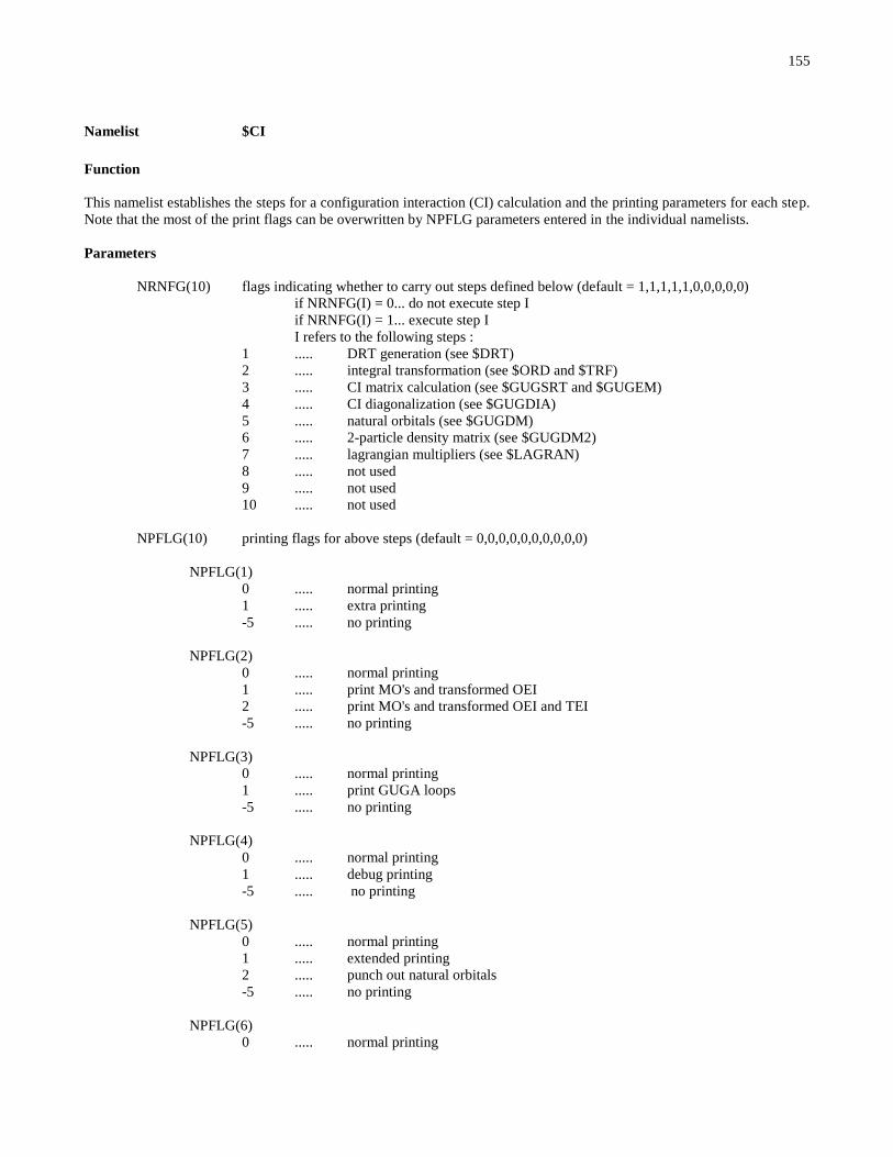
155

Namelist $CI

Function

This namelist establishes the steps for a configuration interaction (CI) calculation and the printing parameters for each step.

Note that the most of the print flags can be overwritten by NPFLG parameters entered in the individual namelists.

Parameters

NRNFG(10) flags indicating whether to carry out steps defined below (default = 1,1,1,1,1,0,0,0,0,0)

if NRNFG(I) = 0... do not execute step I

if NRNFG(I) = 1... execute step I

I refers to the following steps :

1 ..... DRT generation (see $DRT)

2 ..... integral transformation (see $ORD and $TRF)

3 ..... CI matrix calculation (see $GUGSRT and $GUGEM)

4 ..... CI diagonalization (see $GUGDIA)

5 ..... natural orbitals (see $GUGDM)

6 ..... 2-particle density matrix (see $GUGDM2)

7 ..... lagrangian multipliers (see $LAGRAN)

8 ..... not used

9 ..... not used

10 ..... not used

NPFLG(10) printing flags for above steps (default = 0,0,0,0,0,0,0,0,0,0)

NPFLG(1)

0 ..... normal printing

1 ..... extra printing

-5 ..... no printing

NPFLG(2)


1 ..... print MO's and transformed OEI

2 ..... print MO's and transformed OEI and TEI


NPFLG(3)


1 ..... print GUGA loops


NPFLG(4)


1 ..... debug printing


NPFLG(5)


1 ..... extended printing

2 ..... punch out natural orbitals


NPFLG(6)


156

1 ..... print ordered DM2 elements

2 ..... print ordered DM2 elements + debug print for DM2 sorting.

3 ..... print ordered DM2 elements + debug print for DM2 sorting

and print DM2 computation output


NPFLG(7)




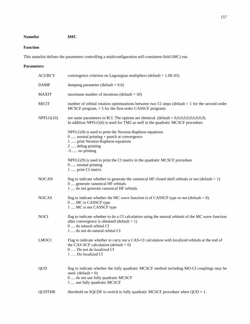
157

Namelist $MC

Function

This namelist defines the parameters controlling a multiconfiguration self-consistent-field (MC) run.

Parameters

ACURCY convergence criterion on Lagrangian multipliers (default = 1.0E-05)

DAMP damping parameter (default = 0.0)

MAXIT maximum number of iterations (default = 30)

MICIT number of orbital rotation optimizations between two CI steps (default = 1 for the second-order

MCSCF program, = 5 for the first-order CASSCF program)

NPFLG(10) see same parameters in $CI. The options are identical. (default = 0,0,0,0,0,0,0,0,0,0).

In addition NPFLG(6) is used for TM2 as well in the quadratic MCSCF procedure.

NPFLG(8) is used to print the Newton-Raphson equations

0 ..... normal printing + punch at convergence

1 ..... print Newton-Raphson equations



NPFLG(9) is used to print the CI matrix in the quadratic MCSCF procedure


1 ..... print CI matrix

NOCAN flag to indicate whether to generate the canonical HF closed shell orbitals or not (default = 1)

0 .... generate canonical HF orbitals

1 .... do not generate canonical HF orbitals

NOCAS flag to indicate whether the MC wave function is of CASSCF type or not (default = 0).

0 .... MC is CASSCF type

1 .... MC is not CASSCF type

NOCI flag to indicate whether to do a CI calculation using the natural orbitals of the MC wave function

after convergence is obtained (default = 1)

0 .... do natural orbital CI

1 .... do not do natural orbital CI

LMOCI Flag to indicate whether to carry out a CAS-CI calculation with localized orbitals at the end of

the CAS-SCF calculation (default = 0)

0 …. Do not do localized CI

1 …. Do localized CI

QUD flag to indicate whether the fully quadratic MCSCF method including MO-CI couplings may be

used. (default = 0)

0 .... do not use fully quadratic MCSCF

1 .... use fully quadratic MCSCF

QUDTHR threshold on SQCDF to switch to fully quadratic MCSCF procedure when QUD = 1.

158

(default = 5.0E-02)

NOAVG This flag can be used when MCSCF calculation is done for an average energy. Then the DM2

matrix corresponds to the average energy expression. This is useful to maintain the spatial

equivalency of the several components of a degenerate state. Sometimes the averaging procedure

is done as a means to obtain convergence for an excited state calculation by avoiding root

flipping.. After the SCF process has converged, it is better to get the DM1 and DM2 matrices for

a pure state, the one that contributes most to the average energy. The energy of the several states

are meaningful, of course, and now the density matrices are too. These energy and density

matrices may be used for natural orbital CI . Since the average orbitals are not the SCF orbitals

of the pure state, they may not be used for a MCSCF gradient calculation as presently

programmed. If NOAVG = 0, the program will not get the density matrices of the pure state, but

will rather use the averaged quantities. If NOAVG = 1, then the program will generate the

quantities for the pure state (default = 0)

FOCAS Flag to use the first-order CAS program (default = 0)

0 .... second-order MCSCF program will be used

1 .... first-order CAS program will be used

CASHFT level shift parameter for first-order CAS program (default = 1.0)

CASDII threshold to turn on the -DIIS- method in the first-order CAS program

(default = 5.0E-02)

NRMCAS flag to turn on the normalization factor in the first-order CAS program (default = 1)

0 ... no normalization of the single excitations is done

1 ... the single excitations are renormalized in the construction of the effective Fock operator

MODTRF flag to select the integral transformation algorithm in the second-order MCSCF program (default

= 2)

1 ... use the ordered AO integrals

2 ... use the unordered AO integrals

MOPRT number of canonical CAS orbitals to be printed; this is valid for the CAS case only since the

canonical CAS orbitals are 'allowed' (default = print doubly occupied and valence orbitals only).

PRTTOL threshold for printing CI coefficients (default = 0.05)

PRTSPN flag to print the spin coupling cases of the configurations (default = 0)

2 … in terms of Slater determinants




6 … in terms of Rumer functions

7 … in terms of Rumer functions

MOFZC number of orbitals that are frozen, i.e. to not change during the SCF process

(default = 0).

Comments

There are three methods used for determining MCSCF wave function: 1. a fully quadratic algorithm for the CI and orbital

rotations; 2. a augmented hessian algorithm, nearly quadratic in the orbital rotations only; 3. and finally a first-order

algorithm. The first two algorithms can treat general MCSCF wave functions, while the third one is valid for CAS wave

functions only.

159

Most often used (also the default) is the augmented hessian matrix approach that treats the orbital-orbital rotations in a

nearly quadratic fashion. It has proven to be a very reliable and stable method, which works in quite many cases. It fails

most often for excited state calculation (see $GUGDM2). We have used it successfully for excited states in several cases

also.

The method usually requires less than 10 iterations to converge, in many cases 4 or 5 iterations. For difficult cases we have

the possibility to use the fully quadratic approach in which both the orbital-orbital rotations and the orbital-CI coupling are

treated at second order. This option is activated by setting QUD = 1.The default value of the convergence criterion

ACURCY may be actually a bit too tight. A value of 1.0E-04 is usually sufficient as the convergence applies to the

Lagrangian multipliers. The variables DAMP and MICIT are rarely used.

The core (doubly occupied) orbitals are not the canonical Hartree-Fock orbitals. It is sometimes useful to generate these

latter orbitals , and this is accomplished by setting NOCAN =0.

The program is not restricted to handling complete active space type of MCSCF wave functions. Sometimes it is

convenient to restrict the excitation level in the valence space. In this case the valence-valence rotations are critical and

must be accounted for. It is mandatory to set NOCAS = 1, otherwise the wave function would not yield the lowest possible

energy after convergence is obtained. This additional step is requested by setting

NOCI = 0.

Sometimes there is a problem associated with this last option: the NO orbitals are obtained by diagonalizing the 1-particle

density matrix, and since the doubly occupied orbitals (MCC) are explicitly treated in this MCSCF program, there may be a

slight mixing of core orbitals belonging to different irreducible representations, which makes the program stop in the

sorting step before doing the NO CI calculation. It is suggested that in these cases NOCI be set to 1.

Five different algorithms are available for the transformation of the AO integrals to the MO basis. First, as described above,

via the MODTRF parameter the user can choose between working directly with the unordered list of AO integrals or

forming the canonically sorted list of AO integrals prior to the transformation step.

When working with the unsorted list of AO integrals, three algorithms are available that differ in their memory and disk

space requirements. The in-memory algorithm is used when at least nN3/2

(n = number of occupied -core and active-

orbitals, N = number of basis functions) words of memory are available in the common /SCM/. No extra disk space is

required in this case; only the unsorted AO integrals file and the MO integrals are needed. When less than nN3/2 but at lest

N3/2 words of memory are available a segmented algorithm is used, transforming the integrals by batches of m occupied

MO orbitals at a time (m being the ratio of the available memory to N3/2). The AO integrals file is read many times (m/n +

1 times) and some extra disk space is needed over the in-memory algorithm. These two methods are the only ones available

when using the direct algorithms (DIRECT=1 in $CNTRL). Finally, when less than N3/2 but at least nN words of memory

are available an out-of-memory transformation is used. An intermediate direct access file (DA20) of size nN2 (N-n/2) is

needed. This algorithm seems to be quite IO expensive and should be avoided. For most situations the automatic selection

made by the program will be adequate and should involve the first two choices. Actually, if you have less than N3/2 words

of memory it is likely that even if the integrals transformation proceed through the out-of-memory algorithm the program

may stop later in the Newton-Raphson rotations.

When working with the ordered list of AO integrals there are only two choices. An ‘in-memory’ algorithm that requires at

least N4/8 words of memory and an ‘out-of-memory’ algorithm that operates when less memory is available. As before a

direct access file is needed in this case and the algorithm is quite IO expensive.

The advantage of working with the ordered list of AO integrals is that all steps in the transformation are matrix

multiplications and the transformation can be done very fast if you have a vector machine. However the exact moment in

which this algorithm is better may depend specifically on the kind of hardware in which you run the program.

The first order CAS program is intended to be used for big calculations in which the integral transformation step and/or the

Newton-Raphson rotations are very cpu and memory expensive. The implementation is based in the method described in:

Meier and Staemmler, Theor.Chim.Acta 76, 95-11 (1989) and is of the renormalized effective Fock operator type. The

main advantage of this algorithm over the second order program is that the integral transformation step is very cheap both

in terms of cpu and memory and also the microiterations are reduced to two one-electron Fock operator transformations and

160

a matrix diagonalization basically. There is a drawback of course and this is the slow convergence of the method. There are

various parameters to control how the orbital rotations are applied but our suggestion is to start with a set of orbitals

relatively close to the final ones (the NO from a limited CI calculation will do it in most cases).

There are two algorithms for the two electrons integrals transformation step. Both of them requires a minimum memory of

at least n2N

2/2 words (now n is only the number of active orbitals) but the first one may need to read the AO integrals file

many times when less than nN3/2 words of memory are available. The program tries to use the first algorithm, but if the AO

integral file needs to be read more than n times, it switches to the second algorithm that needs to read this file only once and

at this point it may be faster.

To perform diabatization, adiabatic wave functions must be CASSCF or MCQDPT type. Therefore NOCAS must be set to

0 (default value) when diabatization in HONDOPLUS is carried out.

161

Namelist $ORD

Function

This namelist controls the integral ordering step before an integral transformation step. The canonical integrals (or

supermatrices) are ordered in square-canonical order: i.e., j .ge.k.ge.l , all kl for a given ij .

Parameters

NDAR number of direct access record on file FT20 (default = 64000)

LDAR record length for direct access file FT20 (default = 4096)

NBOXMX maximum number of boxes used for ordering. (default = 200)

NWORD number of words available as a working area in the integral transformation step. (default = 0 ;

use all available memory)

NPFLG debug printing flag. (default = 0).

0 ..... no printing


Comments

This namelist often does not need to be specified. Its most common usage is for defining the parameters for the direct

access file DA20.

162

Namelist $TRF

Function

This namelist controls the integral transformation step for correlated wave functions.

Parameters

CUTOFF threshold for keeping the transformed integrals on the integral file (default = 1.0E-09)

NPFLG flag to print transformed integrals (default = 0)

0 ..... standard printing, almost none.

1 ..... print MO coefficients and transformed one-electron integrals.

2 ..... print transformed two-electron integrals.

NORDER flag used to indicate whether to reorder the orbitals before the transformation. Note that a similar

feature is available in $GUESS . This option is not active for a MCSCF calculation (default = 0)

0 ..... do not reorder the orbitals

1 ..... reorder the orbitals

IORDER IORDER(I) = J means that orbital J is placed in the I-th position, when NORDER = 1 (default =

canonical order: IORDER(I) = I,I = 1 to 3072).

LDAR record length for direct access file FT20 (default = 4096)

NWORD number of words available as a working area in the integral transformation step

(default = 0 ; use all available memory)

MODTRF parameter used only in the analytic hessian calculation in hss.f (default = 1). It has something to

do with parallel transformation of electron repulsion integrals. See hss.f for deciphering what is

going on.

Comments

This namelist is rarely needed. However, remember that for large basis set calculations, the number of physical records

allocated for the direct access file DA20 may have to be increased as discussed above for $ORD .

The use of NORDER and IORDER should be limited to CI calculations. For MCSCF calculations, the user may convince

himself that using these parameters would highly confuse the program, and in fact these parameters are then ignored by the

code!

163

Data group $DRT

Function

This data group, which also reads as free-format, provides the information about the CI expansion for the Graphical Unitary

Group (GUG) modules that are used for CI and MCSCF calculations.

Cards

CARD 1 FORMAT(10A8)

TITLE(10)

CARD 2 FORMAT(5I5,I3,I2,3I10,I5,I5)

NSYM number of irreducible representations used in the construction of the CI expansion.

Note that the transformed integrals are not blocked by symmetry (default = 1)

NSYM = 0 implies automatic detection of symmetry for $DRT (see Comments below

for explanation)

NORB total number of orbitals used in the CI expansion. The type of these orbitals is described

in the cards CARD3 (default = number of basis functions)

NREFS number of configurations used as a reference and described in the next cards. NREFS

can only be 1 or 2. Usually NREFS = 1, and the reference configuration is the HF

configuration. NREFS = 2 when a GVB pair wave function is used as reference. This is

the only case where NREFS is not equal to 1 (default = 1)

IEXCT maximum level of excitation (default = 0)

NFOCI flag for -first order-, -second order-, ...wave functions. The CI expansion includes the

configurations up to the IEXCT excitation level within the valence orbitals, plus all the

configurations that have up to NFOCI electrons in the external orbitals. (default = 0)

0 ..... this configuration selection option is not in effect

1 ..... first-order CI

2 ..... second-order CI

ICF flag to indicate whether the CI expansion is a interacting correlated fragment CI.

(default = 0)

0 ...... it is not a ICF wave function

1 ...... it is a ICF wave function

INTACT flag to indicate whether to used the interacting space option (default = 0)

0 ...... do not do interacting space.

1 ...... do interacting space.

MXNINT maximum number of integrals in one buffer created by the GUGA program (default =

4096)

MEMEMX maximum number of energy matrix elements per buffer created by the GUGA program.

(default and maximum = 2048)

NWORD size of the working area during DRT generation (default = 0 ; use all available memory)

NPFLG flag to print the list of configuration state functions (default = 0)

164

0 ...... do not print CSF's.

1 ...... print CSF's.

IPP flag to enforce the -perfect pairing- restriction on the valence bond orbital pairs of the

type VBA and VBB (default = 0)

0 ...... do not enforce -perfect pairing -

1 ...... enforce -perfect pairing -

CARD 3 FORMAT(16(A3,I1,1X))

(ORBCOD(I),ISYM(I),I=1,NORB) ORBCOD may be one of the following:

DOC doubly occupied orbital in reference.

UOC unoccupied orbital in reference.

FZC frozen core orbital, doubly occupied in reference and closed in the CI expansion.

FZV frozen virtual orbital, unoccupied in reference and always empty in the CI expansion.

ALP singly occupied orbital in reference with spin.

AOS open shell orbital of an open shell SCF configuration.

BOS open shell orbital of an open shell SCF configuration.

GVA first natural orbital of a GVB pair used as reference configurations.

GVB second natural orbital of a GVB pair used as reference configurations.

VAL orbital that is unoccupied in the reference configuration and is to be included in the

valence space of orbitals.

MCC core orbital of a MCSCF wave function, i.e. it is doubly occupied in all the

configurations. This label is equivalent to FZC.

VBA first orbital of a generalized valence pair. See VBB for further explanation.

VBB second orbital of a generalized valence pair. A total of 2 electrons at most may occupy

one valence pair. The triplet coupled electron pair configuration is included in the list of

configurations when possible. Note that this type of orbital types is more general than

GVA and GVB for which two configurations only are created. Furthermore the GVA,

GVB pair is used only to specify a pair of reference configurations for multireference

CI.

ICA interacting correlated fragment core orbital for fragment -A-

ICB interacting correlated fragment core orbital for fragment -B-

MCA interacting correlated fragment valence orbital for fragment -A-

MCB interacting correlated fragment valence orbital for fragment -B-

Comments

The information inputted in $DRT is aimed at defining the configuration state function (CI) expansion. Two sets of data are

needed: some pieces of information concerning the molecular orbitals, the level of excitation, the type of CI wave function

desired, ... , and one reference configuration, often but not always chosen as the HF configuration. This reference

configuration is specified by means of a description of orbital types, symmetry, and occupancy.

The symmetry types of the orbitals must belong to the cyclic group D2h and its subgroups. The symmetry numbers

(between 1 and NSYM) must satisfy the following convention:

IRREDUCIBLE REPRESENTATION SYMBOLS

ISYM D2h D2 C2h C2v C2 Cs Ci C1

1 AG A Ag A1 A A' Ag A

2 Au B1 Au A2 B A'' Au

3 B3u B3 Bu B1

4 B3g B2 Bg B2

5 B1g

165

6 B1u

7 B2u

8 B3g

As an example we consider the water molecule, assuming a minimal basis set. The data group $DRT could read as follows:

$DRT

H2O (1A1) , CISD

4 7 1 2 0 0 0 1024 1024 0 0 0

DOC1 DOC1 DOC4 DOC1 DOC3 UOC1 UOC4

$END

There are seven orbitals in the orbital set (second parameter in CARD 2) which belong to any of four irreducible

representations of the C2v point group. The orbital description is given in CARD 3. In the reference configuration the first

orbital is doubly occupied and of symmetry 1 (this is the O(1s) orbital), the second orbital has the same characteristics (the

O(2s) orbital), the third orbital is doubly occupied too but of symmetry 4 (the antisymmetric combination of the O- -

orbitals), the fourth orbital is doubly occupied of symmetry 1 (the symmetric combination of O- -orbitals), and finally

the fifth orbital is doubly occupied of symmetry 3 (the out-of-plane O(2p) orbital).The symmetry number of the irreducible

representation of the D2h symmetry point group and subgroups are listed above: for the C2v group 1 corresponds to a1, 2 to

a2, 3 to b1, and 4 to b2. In the reference configuration orbitals 6 and 7 are unoccupied and their symmetry labels are 1 and 4

(they are the symmetric and antisymmetric combinations of the O-

At this point it is good to mention that NSYM = 0is a valid option. Because of the free format input reading, remember that

it is mandatory to have 0 as the first parameter on the card, a blank would confuse the program. In any case, a 0 value of

NSYM tells the program to recognize by itself the number of irreducible representations, and later it will automatically

assign the irrep number to each orbital, over-writing the input data. Thus the data group $DRT could read as follows:

$DRT

H2O (1A1) , CISD

0 7 1 2 0 0 0 1024 1024 0 0 0

DOC DOC DOC DOC DOC UOC UOC

$END

and the program would figure out the symmetry of each orbital. Note that the orbital codes for the $DRT can be read in a

free format whereby a multiplicative number can be read in front of an orbital code. Thus the data group $DRT could now

read as follows:

$DRT

H2O (1A1) , CISD

0 7 1 2 0 0 0 1024 1024 0 0 0

5*DOC 2*UOC

$END

The only concern at this point is for the user to be sure that the orbitals coming into the DRT are indeed of the right orbital

code, which may require or not to reorder the orbitals through the NORDER parameter in $GUESS. Similar input forms

can be used for all the examples discussed below. We will give one more taste of free format in the next example, and will

stick to the old notation thereafter.

The third parameter of CARD 2 indicates that only one reference configuration is used, and it is the one specified by CARD

3. The fourth parameter indicates that the highest level of excitations in the generation of the CI configurations is two.

Electrons are promoted from the doubly occupied orbitals into the unoccupied orbitals. This is a singles + doubles CI.

To freeze the core electrons O(1s), it suffices to specify the first orbital as FZC1. It is now a frozen core orbital. Eliminating

virtual orbitals can be done by reducing the value of the second argument on CARD 2 or by specifying orbitals of the type

FZV

166

Consider now CH2(3B1) for a singles + doubles CI. The $DRT input would look like this:

$DRT

CH2 (3B1) , CISD

4 7 1 2 0 0 0 1024 1024 0 0 0

FZC1 DOC1 DOC4 ALP3 ALP1 UOC1 UOC4

$END

or equivalently for automatic assignment of symmetry:

$DRT

CH2 (3B1) , CISD

0 7 1 2 0 0 0 1024 1024 0 0 0

FZC 2*DOC 2*ALP 2*UOC UOC

$END

The meaning of the parameters on CARD 2 has just been given. The only new things are the two orbitals labeled ALP3

ALP1. They are the singly occupied orbitals in the HF configuration of the system. The configuration specified here is

indeed a triplet state, and all the excited configurations will also have triplet spin. The symmetry of the state is B1 and all

the excited configurations will also have that symmetry. Electrons are promoted from the DOC and ALP orbitals into the

virtual orbitals. The C(1s) electrons are frozen.

Consider now CH2(1A1) for which we want to generate single and double excitation from two configurations. The input

data should look like this:

$DRT

CH2 (1A1) , CISD2

4 7 2 2 0 0 0 1024 1024 0 0 0

FZC1 DOC1 DOC4 GVA3 GVB1 UOC1 UOC4

$END

This is the only case where the third parameter on CARD 2 takes the value of 2. It requires that two orbitals be specified as

GVA and GVB. The first five orbitals define the two configurations used as references from which excitations are

performed.

The data for CH2(1B1) would look like this:

$DRT

CH2 (1B1) , CISD

4 7 1 2 0 0 0 1024 1024 0 0 0

FZC1 DOC1 DOC4 AOS3 BOS1 UOC1 UOC4

$END

Consider again CH2(1A1) for which we want to do a 2 configuration MCSCF calculation:

$DRT

CH2 (1A1) , 2-CASSCF

4 5 1 2 0 0 0 1024 1024 0 0 0

MCC1 MCC1 MCC4 DOC3 VAL1 UOC1 UOC4

$END

Even though we specified seven orbitals, note that only five are used in the CI expansion because of the value of the second

parameter on CARD 2. The MCC labels indicate that these three orbitals are doubly occupied in all the configurations

generated for the CI expansion used in the MCSCF calculation. They play the same role as the FZC labels. Up to double

excitations among orbitals 4 and 5 are created. A larger configuration set can be obtained with the following data:

167

$DRT

CH2 (1A1) , 6-CASSCF

4 7 1 6 0 0 0 1024 1024 0 0 0

MCC1 DOC1 DOC4 DOC3 VAL1 VAL1 VAL4

$END

Other orbital types are available. Specific applications will require these capabilities. It is however difficult to give a fully

comprehensive description of all the options provided. The one presented above cover a widely class of applications.

Note that for all these cases the orbital list given on CARD 3 must match the order in which the orbitals will be found

before the integral transformation step, otherwise a mismatch will occur and the program is likely to stop in the $GUGSRT

step if symmetry is used. It could be that the program will not stop because no symmetry is used or because of lucky (or

rather unlucky) coincidence, only a weird energy would indicate that something is wrong.

168

Namelist $GUGSRT

Function

This namelist controls the sorting of the transformed electron repulsion integrals (TEI) for use in the GUGA CI program.

Parameters

NDAR number of direct access records available on FT20 in the integral sorting step

(default = 64000)

LDAR length for a record on the direct access file FT20 (default = 4096)

NBOXMX maximum number of boxes allowed in the sorting step (default = 200)

NWORD size of available working area for sorting step (default = 0 ; use all available memory)

NPFLG flag to print GUGA-ordered integrals (default = 0)

0 ....... standard printing, almost none

1 ....... print GUGA-ordered MO integrals

Comments

The same comment found in $ORD about the direct access file DA20 applies.

169

Namelist $GUGEM

Function

This namelist controls the calculation of the CI matrix file in the original formulation of the Graphical Unitary Group

Approach (GUGA) CI method.

Parameters

NWORD size of available working area for creation of the diagonalization tape by the GUGA program.


CUTOFF threshold value for keeping the diagonalization tape contributions (default = 1.0E-08)

NPFLG flag to print GUGA loops and indices (default = 0)


1 ....... print GUGA loops

GUGFML flag to store the value of the GUGA loops on FT14. Indeed the same loops are used for the

diagonalization tape, the 2-particle density (DM2) matrix elements, and the 2-particle transition

(TM2) matrix elements. Storing of the loops can result in significant CPU time saving (default =

0)

0 ....... do not store loop values.

1 ....... store loop values.

NFML number of loops stored in each record of FT14 when GUGFML = 1. (default = 1024)

GUGFIL this parameter is used to indicate whether FT14 exists before the start of the present run. If it

does exist (GUGFIL .NE. 0), then the program will try to use it. If it does not exist (GUGFIL

.EQ. 0), then the program will not try to use it of course, and will open a new file. If the file is on

disk, but GUGFIL .EQ. 0 , the program will use the existing disk space, but it will open a new

file (default = 0)

170

Namelist $GUGDIA

Function

This namelist controls the diagonalization of the CI matrix, which actually does not quite exist as a matrix. See the original

GUGA approach for information. Only when the CI matrix is small enough can one find it as such in memory.

Parameters

NDAVID when possible (enough memory), the diagonalization of the CI matrix is done in memory. The

root finding method of Davidson-Liu is used, in memory or out of memory (default = 0)

0 ..... program decides upon in-memory or out-of-memory solution.

1 ..... force out-of-memory solution

NWORD size of the available working area for solving the eigenvalue problem in the CI calculation


NPFLG flag for debug printing (default = 0)


1 ....... extended printing

NSTATE number of roots to be found (default = 1 , maximum = 50)

MNXPAN minimum size of the expansion vector set used in the iterative method for finding eigenvalues

and eigenvectors (default = 1)

MXXPAN maximum size of the expansion vector set used in the iterative method for finding eigenvalues

and eigenvectors (default = 30)

MAXIT maximum number of iterations allowed in the eigenvalue finding iterative method (default = 50)

CVGTOL convergence threshold for the iterative method (default = 5.0E-06)

PRTTOL threshold for printing the CI coefficients (default = 1.0E-02)

NOVEC for the CI diagonalization the program checks FT12 for initial guess vectors. If there are

MNXPAN such vectors, then they are used as expansion vectors in the iterative method If there

are no vectors, or fewer than MNXPAN, then the program generates a set if initial expansion

vectors. NOVEC is used to force the program to generate the initial guess vectors, even if

enough vectors are available from FT12 (default = 0)

0 ..... program may use FT12 vectors.

1 ..... program may not use FT12 vectors.

DIAFIL this parameter is used to indicate whether FT12 exists before the start of the present run. If it

does exist (DIAFIL.NE.0), then the program will try to use it. If it does not exist

(DIAFIL.EQ.0), then the program will not try to use it of course, and will open a new file. If the

file is on the disk, but DIAFIL.EQ.0, the program will use the existing disk space, but it will

open a new file (default = 0)

NCORE Force in-memory Davidson's diagonalization or dense matrix diagonalization

(default = 0)

0 …. in-memory Davidson's method

1 …. Dense matrix diagonalization

Comments

171

In some rare instances the iterative diagonalization appears to find no improved expansion vector and yet the

diagonalization has not converged. In that case the program tells you to increase the value of CVGTOL. One should look at

the behavior of the iterative process and modify this parameter accordingly.

172

Namelist $GUGDM

Function

This namelist controls the calculation of the one-particle density matrix (DM1) and of the natural orbitals (NO) from the

GUGA-CI wave function.

Parameters

ISTATE(50) flag to indicate whether to calculate the natural orbitals of the I-th CI state

(default = 1, 49* 0)

ISTATE(I) = 0 ..... do not get NO's

ISTATE(I) = 1 ..... get NO's

NWORD size of the available working area for calculating the natural orbitals (default = 0; use all

available memory)

Comments

To punch out the natural orbitals, see NPFLG(5) in $CI.

If the $GUGDM namelist is used with the $GUGDM2 namelist, it must always occur prior to the $GUGDM2 namelist in

the input file.

173

Namelist $GUGDM2

Function

This namelist controls the one-and two-particle density matrix (DM1 and DM2) evaluation from a CI wave function. It

also plays a key role in MCSCF calculations as it is the means to specify the electronic state(s) for which the wave function

is calculated. Calculations on excited states and calculations on average states may be performed. Examples for these are

given below.

Parameters

NSTATE number of CI states included in the average state wave function for which the DM2 is to be

calculated. The serial number of the states included is given in ISTATE and the corresponding

weights in WSTATE (see below). If NSTATE = 1 , then the DM2 is calculated for the pure state

whose serial number is ISTATE(1) (default = 1)

ISTATE(50) serial number of the states contributing to the average state for which the DM2 is to be obtained.

The corresponding weights are given in WSTATE (see below)

(default = 1, 49*0)

WSTATE(50) weights of the CI states contributing to the average state. WSTATE(I) is the weight of the state

with serial number ISTATE(I) (default =1., 49* 0.)

NWORD size of the available working area for calculating the 2-particle density matrix of the CI

expansion (default = 0 ; use all available memory)

NORDER flag to put DM2 in canonical order. Whether DM2 is ordered or not, it is written to file FT15.

For a MCSCF wave function calculation only, DM2 may not be in canonical order. If the energy

gradient is calculated after the wave function calculation then DM2 must be in canonical order

(default = 0)

0 ..... order DM2 to canonical order.

1 ..... do not order DM2

NDAR number of records available on direct access file FT20 for ordering DM2

(default = 4000)

LDAR record length on FT20 .(default = 4096)

NBOXMX maximum number of boxes to be used in ordering DM2 (default = 200)

Comments

The default setting is for a calculation on the ground state of spatial and spin symmetry corresponding to the wave function

description given in the data group $DRT. It is equivalent to the following input:

$GUGDM2 NSTATE=1, ISTATE=1, $END

For a calculation on an excited state of same spatial and spin symmetry as specified in $DRT, the following input may be

used:

$GUGDM2 NSTATE=1, ISTATE=2, $END

An equivalent specification is :

$GUGDM2 NSTATE=2, ISTATE=1,2, WSTATE=0.0, 1.0, $END

174

The specification of an average state calculation is very similar to this latter input, and is as follows:

$GUGDM2 NSTATE=2 , ISTATE=1,2, WSTATE=0.1, 0.9, $END

which indicates that the contribution of state 1 to the DM2 has a weight of 10% , and the contribution from state 2 has a

weight of 90% .

Note that excited state calculations do not always converge. There are cases where the program works very well though. It

is our experience that even an extremely small weight for the lower state as shown in the example above is sufficient to

make the excited state calculation converge.

Remember that another way to converge an excited state calculation is to turn on the fully quadratic MCSCF method using

the input parameters available in $MC. The present program however can not handle very large CI expansion in this

quadratically convergent technique, because the system of linear equations, although solved iteratively, is constructed in

memory.

If the $GUGDM2 namelist is used with the $GUGDM namelist, the $GUGDM namelist must always occur before the

$GUGDM2 namelist in the input file.

175

Namelist $NEWTON

Function

This namelist controls the construction of the orbital gradient and hessian that determine the orbital rotations in a MCSCF

calculation.

Parameters

NWORD size of the available working area for constructing the Newton-Raphson equations in a MCSCF

calculation. (default = 0 ; use all available memory)

NPFLG debug printing flag (default = 0).

0 ..... no printing


NOROT(2,250) orbital pair rotation flag, indicating whether the Newton-Raphson parameters corresponding to a

given pair of orbitals need be calculated.

NOROT=I1,J1, I2,J2, I3,J3,means that the rotations (I1,J1),(I2,J2),(I3,J3) will not be set up in

the Newton-Raphson equations. I is the row index, running from 1 to NORB, and J is the

column index running from 1 to MAX0(I,-NVAL-), where -NVAL- is the number of occupied

(core + valence) orbitals (default = 500*0)

NDIAG flag to select diagonalization method for the Augmented Hessian matrix (default = 0)

0 ..... Davidson's iterative method is used.

1 ..... in memory diagonalization is used.

CVGTOL convergence threshold for Davidson's algorithm (default = 1.0E-05)

Comments

Davidson's method is used to find eigenvalues and eigenvectors of the Augmented Hessian Matrix, which is the core of the

MCSCF orbital optimization algorithm. The method is used by default, but because of the structure of the matrix (not

diagonally dominant) it may fail. There are then two choices to proceed: 1. change the convergence threshold CVGTOL to

a larger value; 2. use the other method by changing NDIAG.

One of the possibly useful features is the ability to force out rotations between specific pairs of orbitals, in some particular

situations, using the input variables NOROT. Of course default situations exist, for example when the wave function is of

the COMPLETE ACTIVE SPACE type, also labeled FORS type, and also sometimes called Full valence CI type. In these

cases rotations among the active orbitals (or valence orbitals) do not change the energy and therefore do not need to be

calculated. The cases are flagged with the variable NOCAS = 0 in the namelist $MC. The program skips the active-active

rotations automatically, just like it does for the core-core rotations.

176

Namelist $TRFDM2

Function

This namelist is NOT USED presently.

This namelist is related to the transformation of the two particle density matrix DM2 from the MO basis to the AO basis

for use in energy derivatives calculations.

Parameters

NDAR number of records available on direct access file FT20 for out-of-memory DM2 transformation

(default = 64000)

LDAR record size on FT20 (default = 4096)

NBOXMX maximum number of boxes per pass to be used for sorting transformed DM2 elements for

derivative calculations (default = 200)

NWORD size of the available working area for DM2 transformation

(default = 0. use all available memory)

CUTOFF threshold for storing transformed DM2 elements on disk file (default = 1.0E-09)

NPFLG print and debug flag (default = 0)

0 ..... no printing

1 ..... print main data and transformed DM2

2 ..... print main data and transformed DM2 + debug print in DM2 sorting.

177

Namelist $CPHF

Function

This namelist gives an option for the integral transformation for the CPHF in the analytic hessian RHF SCF module.

Parameters

NOTRF option for integral transformation algorithm for CPHF of analytic hessian (default = 0)

0 …. CPHF in MO basis

1 …. CPHF in AO basis

Comments

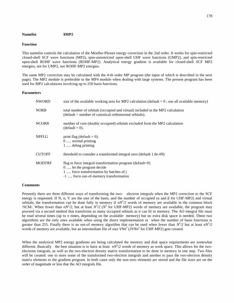
178

Namelist $MP2

Function

This namelist controls the calculation of the Moeller-Plesset energy correction in the 2nd order. It works for spin-restricted

closed-shell SCF wave functions (MP2), spin-unrestricted open-shell UHF wave functions (UMP2), and spin-restricted

open-shell ROHF wave functions (ROHF-MP2). Analytical energy gradient is available for closed-shell SCF MP2

energies, not for UMP2, nor ROHF-MP2 energies.

The same MP2 correction may be calculated with the 4-th order MP program (the input of which is described in the next

page). The MP2 module is preferable to the MP4 module when dealing with large systems. The present program has been

used for MP2 calculations involving up to 250 basis functions.

Parameters

NWORD size of the available working area for MP2 calculation (default = 0 ; use all available memory)

NORB total number of orbitals (occupied and virtual) included in the MP2 calculation

(default = number of canonical orthonormal orbitals).

NCORB number of core (doubly occupied) orbitals excluded from the MP2 calculation

(default = 0).

NPFLG print flag (default = 0).



CUTOFF threshold to consider a transformed integral zero (default 1.0e-09)

MODTRF flag to force integral transformation program (default=0)

0 ..... let the program decide

1 ..... force transformation by batches of j

-1 ..... force out-of-memory transformation

Comments

Presently there are three different ways of transforming the two- electron integrals when the MP2 correction to the SCF

energy is requested. If N, n, V are the size of the basis, and the number of occupied (α and β for UHF-MP2) and virtual

orbitals, the transformation can be done fully in memory if nN3/2 words of memory are available in the common block

/SCM/. When fewer than nN3/2, but at least N

3/2 (N

3 for UHF-MP2) words of memory are available, the program may

proceed via a second method that transforms as many occupied orbitals as it can fit in memory. The AO integral file must

be read several times (up to n times, depending on the available memory) but no extra disk space is needed. These two

algorithms are the only ones available when using the direct implementation or when the number of basis functions is

greater than 255. Finally there is an out-of memory algorithm that can be used when fewer than N3/2 but at least nN

2/2

words of memory are available, but an intermediate file of size VNn2 (3VNn

2 for UHF-MP2) gets created.

When the analytical MP2 energy gradients are being calculated the memory and disk space requirements are somewhat

different. Basically the best situation is to have at least nN3/2 words of memory as work space. This allows for the two-

electrons integrals, as well as the two-electron density matrix transformation to be done in memory in one step. Two files

will be created: one to store some of the transformed two-electron integrals and another to pass the two-electron density

matrix elements to the gradient program. In both cases only the non-zero elements are stored and the file sizes are on the

order of magnitude or less that the AO integrals file.

179

The MP2 gradient program has a minimum memory requirement of N3/2 words of memory as working space. When fewer

than nN3/2 (but at least N

3/2) words of memory are available the programs proceeds by batches of m occupied orbitals at a

time (m being the ratio of the available memory to N3/2) reading the AO integrals file several times. The two-electron

density matrix transformation proceeds in a similar way and has similar memory requirements, but in this case the two-

electron integrals derivatives have to be calculated for each batch and the cpu time will increase significantly if the

available memory is small in comparison with the size of the calculation. In any case no extra disk space above the

previously discussed amount will be needed.

The CUTOFF parameter is used to discard small integrals in some places in the course of the calculation. In the energy-

only program this may reduce the amount of cpu used by discarding the contribution of some integrals to the energy. In the

MP2-gradient program this parameter is used as well for keeping the transformed integrals on the integral file.

180

Namelist $MP4

Function

This namelist controls the calculation of the Moller-Plesset energy corrections up to 4-th order. This is only for spin-

restricted closed-shell SCF wave functions. Note that if you are interested in the second order correction only, you may be

better off using the MP2 module, (the input of which was described in the page ahead of the present one).

Parameters

MP order of MP calculation. (default = 4)

2 ..... MP2 calculation

3 ..... MP2 + MP3 calculation

4 ..... MP2 + MP3 + MP4 calculation

NORB number of orbitals used in the calculation. It is the number of frozen orbitals (see NCORB) + the

number of occupied orbitals + the number of virtual orbitals. It does not include the number of

deleted virtual orbitals (default = number of basis functions)

NCORB number of frozen core orbitals. (default = 0)

NOTRIP flag to indicate whether to calculate the contribution of triple excitations to the 4-th order

energy. (default = 0)

0 ..... do triples

1 ..... do not do triples

NDAR number of logical direct access records for file FT30 (default = 2000)

NWORD size of the available working area for the MP calculation (default = 0 ; use all available memory)

NPFLG printing flag (default = 0)



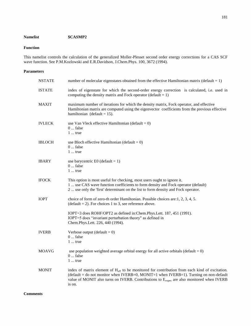
181

Namelist $CASMP2

Function

This namelist controls the calculation of the generalized Moller-Plesset second order energy corrections for a CAS SCF

wave function. See P.M.Kozlowski and E.R.Davidson, J.Chem.Phys. 100, 3672 (1994).

Parameters

NSTATE number of molecular eigenstates obtained from the effective Hamiltonian matrix (default = 1)

ISTATE index of eigenstate for which the second-order energy correction is calculated, i.e. used in

computing the density matrix and Fock operator (default = 1)

MAXIT maximum number of iterations for which the density matrix, Fock operator, and effective

Hamiltonian matrix are computed using the eigenvector coefficients from the previous effective

hamiltonian (default = 15).

IVLECK use Van Vleck effective Hamiltonian (default = 0)

0 ... false

1 ... true

IBLOCH use Bloch effective Hamiltonian (default = 0)

0 ... false

1 ... true

IBARY use barycentric E0 (default = 1)

0 ... false

1 ... true

IFOCK This option is most useful for checking, most users ought to ignore it.

1 ... use CAS wave function coefficients to form density and Fock operator (default)

2 ... use only the 'first' determinant on the list to form density and Fock operator.

IOPT choice of form of zero-th order Hamiltonian. Possible choices are:1, 2, 3, 4, 5.

(default = 2). For choices 1 to 3, see reference above.

IOPT=3 does ROHF/OPT2 as defined in:Chem.Phys.Lett. 187, 451 (1991).

IOPT=5 does “invariant perturbation theory" as defined in

Chem.Phys.Lett. 226, 440 (1994).

IVERB Verbose output (default = 0)

0 ... false

1 ... true

MOAVG use population weighted average orbital energy for all active orbitals (default = 0)

0 ... false

1 ... true

MONIT index of matrix element of Heff to be monitored for contribution from each kind of excitation.

(default = do not monitor when IVERB=0, MONIT=1 when IVERB=1). Turning on non-default

value of MONIT also turns on IVERB. Contributions to Eexpec are also monitored when IVERB

is on.

Comments

182

See above reference for detail discussion of the formalism.

Remember to set the wave function flag WFNFGL=10 in the namelist $WFN. The program works within a fixed spin and

symmetry-adapted subspace, so all roots have the desired spin and symmetry. The method assumes a CASSCF wave

function as specified in $DRT, and canonical orbitals ought to have been requested in $MC. Among the types of orbitals

given in $DRT, the FZC orbitals are not correlated in the CAS-MP2 calculation, while the MCC orbitals are correlated. The

spin and symmetry are taken from $DRT.

183

Namelist $MCQDPT

Function

This namelist controls the Multi-reference Quasi-degenerate-perturbation Theory module developed by H. Nakano and K.

Hirao, University of Tokyo. The intruder state avoidance (ISA) method was taken from GAMESS and is explained in H.A.

Witek, Y.-K. Choe, J.P. Finley, and K. Hirao, J. Comp. Chem. 23, 957 (2002). For examples of how intruder states appear

at some points on the PES see K.R. Glaesemann, M.S. Gordon, and H. Nakano, Phys. Chem. Chem. Phys. 1, 967 (1999)

and H.A. Witek, D.G. Fedorov, K. Hirao, A. Viel, and P.-O. Widmark, J. Chem. Phys. 117, 8396 (2002).

Parameters

NEL # of electrons

MULT Spin multiplicity

NMOFZC # of frozen core orbitals (not correlated in PT)

NMODOC # of doubly occupied orbitals (correlated in PT)

NMOACT # of active orbitals

NMOEXT # of external orbitals

NSTATE # of target state(s) ( = Dimension of effective Hamiltonian )

ISTSYM State symmetry of target state(s)

INORB Read input orbitals from cards (1) or from the direct access file DA10

INOFMT

LPOUT Print option in MC-QDPT

0:Normal print

<0:Debug print (-1,-5,-10,-100)

NSTCI # of states to be obtained in the Davidson's method

KSTATE State is used (1) or not (0) in MC-QDPT2 (1-d array)

THRENE Threshold for the energy convergence in the Davidson's method

THRCON Threshold for the vector convergence in the Davidson's method

IFORB Redefine canonical Fock orbitals (1) or not (0)

AVECOE Weight of the each state in computing (averaged) density matrix (1d array)

THRGEN Threshold for one-, two-, three-particle coupling constants in the perturbation

calculation. Note: If you want, for example, to obtain energies to 6 figures after point,

set thrgen=1.0d-8 or 1.0d-9.

MAXROW Maximum # of row in the distinct row table (DRT)

184

MAXCSF Maximum length for one-particle coupling constant used in CAS-CI calculation

(maxcsf<ncsf is permissible).

LENGTH Buffer length for the coupling constant io

THRERI Threshold to keep ERIs on MO base

MXTRFR Maximum number of reads in the integral transformation step

MAXERI Buffer length for 2-electron integral IO

NSOLUT # of states to be solved in the Davidson's method. Note: Used in the isym=0 case.

NSTOP Maximum # of iteration in the Davidson's method

MXBASE Maximum # of basis vector in the Davidson's method

MDI Dimension of small Hamiltonian used in setting initial vector(s) in the Davidson's

method

THRENE Threshold for the energy convergence in the Davidson's method

THRCON Threshold for the vector convergence in the Davidson's method

MAINCS CSFs belonging to the symmetry of the target state(s) Note: Used in the isym=0 case.

(1-d array)

ISELCT Select CSF (1) or not (0)

THRWGT Threshold weight (=/Ci/**2) for CSF selection

NPCONF # of parent configurations

MAXEX Maximum # of excitations out of parent configurations

LPCONF Labels of parent orbital configurations (1-d array). Note: See output file ft66.

IROT Use MP2 formula for the (dd)->(ee) excitations (1) or not (0). Note: Set irot=1 in

MRMP2 and irot=0 in MC-QDPT2.

IWGT Calculate contribution to the effective Hamiltonian and weight(s) of the reference

(zero-th order) state(s) (1) or not (0). Note: More memory is used than in the case

iwgt=0, and it takes about 2-3 times CPU time.

MODE Mode for MC-QDPT2 calculation

1: Standard mode

2: Debug mode

THRGEN Threshold for one-, two-, three-particle coupling constants in the perturbation

calculation. Note: If you want, for example, to obtain energies to 6 figures after the

decimal point, set thrgen=1.0d-8 or 1.0d-9.

GENZRO Zero threshold for one-, two-, and three-particle coupling constant calculations

185

IDIPO Calculate (electronic) dipole and transition dipole moment (1) or not (0) at CAS-CI

level. Note: This does not yield correct values in the version working inside HONDO.

Note2: Does not include the contribution from nuclear charges.

IQDCHK Check quasi-degeneracy (1) or not (0)

THQDC2 Threshold of the coefficients of reference CSFs to be printed out

THQDEO Threshold of the difference of energy denominator to be printed out

EDSHFT Value of denominator energy shift used by the intruder-state-avoidance (ISA) method.

Comments

Example. If you want the second and the fourth roots, set

nstate=2, nstci=4, kstate=0,1,0,1, .

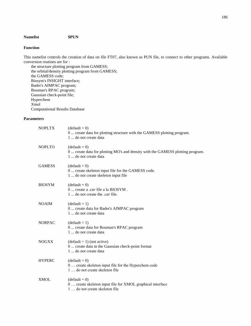
186

Namelist $PUN

Function

This namelist controls the creation of data on file FT07, also known as PUN file, to connect to other programs. Available

conversion routines are for :

the structure plotting program from GAMESS;

the orbital/density plotting program from GAMESS;

the GAMESS code;

Biosym's INSIGHT interface;

Bader's AIMPAC program;

Bouman's RPAC program;

Gaussian check-point file;

Hyperchem

Xmol

Computational Results Database

Parameters

NOPLTX (default = 0)

0 ... create data for plotting structure with the GAMESS plotting program.

1 ... do not create data

NOPLTO (default = 0)

0 ... create data for plotting MO's and density with the GAMESS plotting program.


GAMESS (default = 0)

0 ... create skeleton input file for the GAMESS code.

1 ... do not create skeleton input file

BIOSYM (default = 0)

0 ... create a .car file a la BIOSYM .

1 ... do not create the .car file.

NOAIM (default = 1)

0 ... create data for Bader's AIMPAC program


NORPAC (default = 1)

0 ... create data for Bouman's RPAC program


NOGXX (default = 1) (not active)

0 ... create data in the Gaussian check-point format


HYPERC (default = 0)

0 … create skeleton input file for the Hyperchem code

1 … do not create skeleton file

XMOL (default = 0)

0 … create skeleton input file for XMOL graphical interface

1 … do not create skeleton file

187

CRDB (default = 0)

0 … create flat ASCII file for Computational Results Database

1 … do not create flat ASCII file

188

Namelist $PRP

Function

This namelist controls the calculation of electronic properties. Available properties are:

dipole moment;

quadrupole moment;

octupole moment;

population analysis and spin population;

localized orbitals via Boys' method;

polarizability and hyper-polarizabilities;

frequency dependent (hyper)polarizabilities;

(hyper)polarizabilities by sum-over-states;

spin and electron density maps, and orbital wave function maps;

electrostatic potential maps;

electrostatic fields at the nuclei;

electrostatic field gradients at the nuclei;

hyperfine interactions (Fermi contact term and anisotropic interaction);

Stone's distributed multipole analysis;

NMR chemical shifts by GIAO formalism;

potential-derived charges

Parameters

NODIP (default = 0)

0 ... calculate dipole

1 ... do not calculate dipole

NOQDP (default = 1)

0 ... calculate quadrupole

1 ... do not calculate quadrupole

NOOTP (default = 1)

0 ... calculate octupole

1 ... do not calculate octupole

NOPOP (default = 0)

0 ... Mulliken population and bond order analysis

1 ... skip population analysis

NOSTON (default = 0) see data group $STONE

0 ... Stone's distributed multipole analysis

1 ... skip Stone's analysis

NODEN (default = 1) see namelist $MAP

0 ... electron and spin density, or orbital wave function maps

1 ... skip densities evaluation

NOELP (default = 1) see namelist $MAP

0 ... electrostatic potential mapping.

1 ... skip electrostatic potential mapping

NOELF (default = 1)

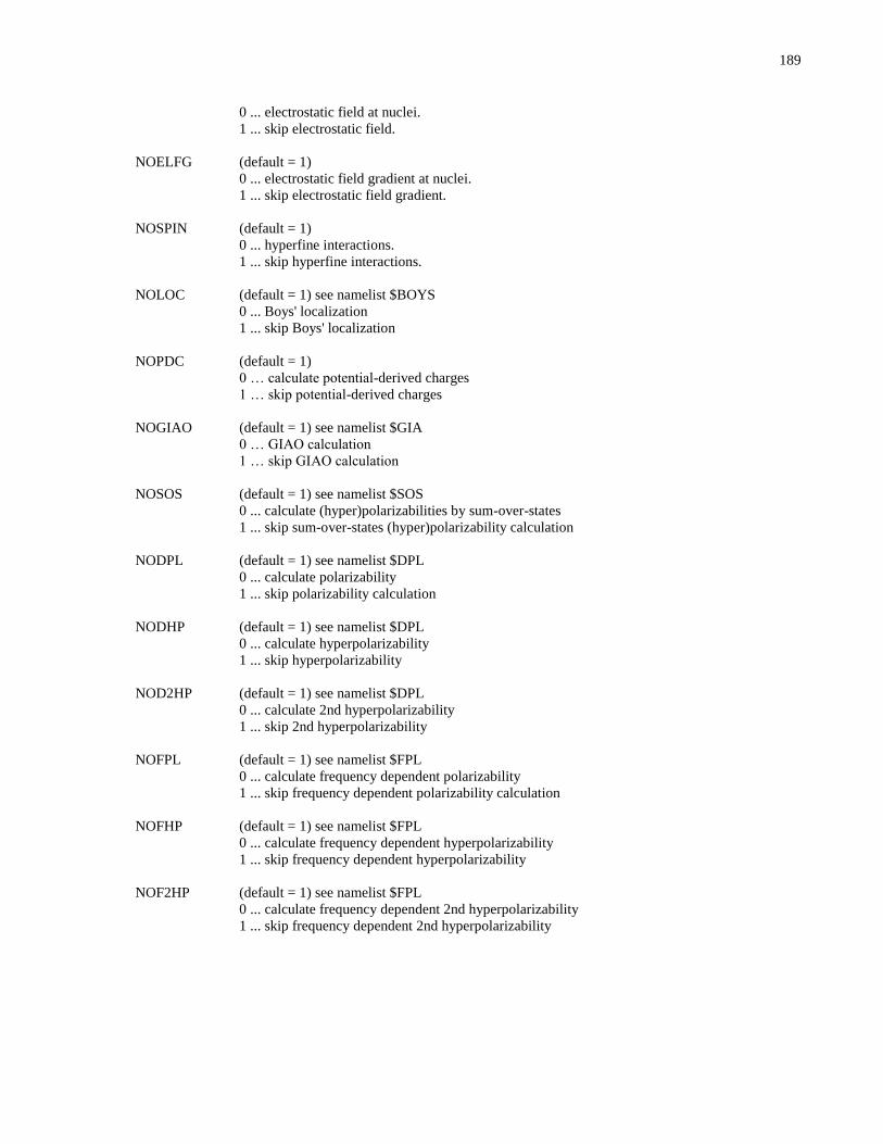
189

0 ... electrostatic field at nuclei.

1 ... skip electrostatic field.

NOELFG (default = 1)

0 ... electrostatic field gradient at nuclei.

1 ... skip electrostatic field gradient.

NOSPIN (default = 1)

0 ... hyperfine interactions.

1 ... skip hyperfine interactions.

NOLOC (default = 1) see namelist $BOYS

0 ... Boys' localization

1 ... skip Boys' localization

NOPDC (default = 1)

0 … calculate potential-derived charges

1 … skip potential-derived charges

NOGIAO (default = 1) see namelist $GIA

0 … GIAO calculation

1 … skip GIAO calculation

NOSOS (default = 1) see namelist $SOS

0 ... calculate (hyper)polarizabilities by sum-over-states

1 ... skip sum-over-states (hyper)polarizability calculation

NODPL (default = 1) see namelist $DPL

0 ... calculate polarizability

1 ... skip polarizability calculation

NODHP (default = 1) see namelist $DPL

0 ... calculate hyperpolarizability

1 ... skip hyperpolarizability

NOD2HP (default = 1) see namelist $DPL

0 ... calculate 2nd hyperpolarizability

1 ... skip 2nd hyperpolarizability

NOFPL (default = 1) see namelist $FPL

0 ... calculate frequency dependent polarizability

1 ... skip frequency dependent polarizability calculation

NOFHP (default = 1) see namelist $FPL

0 ... calculate frequency dependent hyperpolarizability

1 ... skip frequency dependent hyperpolarizability

NOF2HP (default = 1) see namelist $FPL

0 ... calculate frequency dependent 2nd hyperpolarizability

1 ... skip frequency dependent 2nd hyperpolarizability

190

Namelist $MLK

Function

This namelist can be used to over-write the number of molecular orbitals for which the Mulliken Population analysis is

carried out. The default is the number of occupied orbitals. Sometimes it is useful to do the analysis for some unoccupied

orbitals.

Parameters

NORB number of orbitals for which the Mulliken Population analysis is done (default = 0, use all the

occupied orbitals).

MOFLG flag to specify which orbital set to use in the population analysis for MCSCF or CI wave

functions (default = 0)

0 ... use natural orbitals of the MC or CI wave function

1 ... use the MC orbitals (possibly canonical Fock orbitals)

Comments

The use of this namelist is rather straightforward.

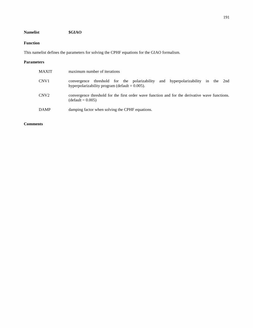
191

Namelist $GIAO

Function

This namelist defines the parameters for solving the CPHF equations for the GIAO formalism.

Parameters

MAXIT maximum number of iterations

CNV1 convergence threshold for the polarizability and hyperpolarizability in the 2nd

hyperpolarizability program (default = 0.005).

CNV2 convergence threshold for the first order wave function and for the derivative wave functions.

(default = 0.005)

DAMP damping factor when solving the CPHF equations.

Comments

192

Namelist $DPL

Function

Controls the calculation of polarizabilities and hyperpolarizabilities via the Coupled Perturbed Hartree-Fock (CPHF)

method implemented in a iterative fashion. This is presently implemented only for closed-shell wave functions. For CPHF

equations see : C. Dykstra, P. Jasien, Chem. Phys. Lett. 109, 388 (1980).

The first derivative of the wave function with respect to an electric field yields polarizability and first hyperpolarizability.

The second hyperpolarizability requires the second order CPHF.

(Hyper)polarizability tensor components are output in the input cartesian coordinate system, the coordinate system of the

inertial axes, and if the polarizability tensor is calculated, in the coordinate system for which the polarizability tensor is

diagonal.

Parameters

MAXIT maximum number of iterations for each direction (default = 50)

CNV1 convergence threshold for the polarizability and hyperpolarizability in the 2nd

hyperpolarizability program (default = 0.005).

CNV2 convergence threshold for the first order wave function and for the derivative wave functions.

(default = 0.005)


0 ... normal print

1 ... print transformation matrix (U matrix) and density derivative matrix.

2 ... debug printing for the first and second hyperpolarizabilities.

XDAMP damping factor for the derivative density matrix for the x-direction

(default = 0.2) (XDAMP = 0.2 means 0.2 old+0.8 new)

YDAMP damping factor for the derivative density matrix for the y-direction (default = 0.2)

ZDAMP damping factor for the derivative density matrix for the z-direction (default = 0.2)

XXDAMP, XYDAMP, XZDAMP, YYDAMP, YZDAMP, ZZDAMP

damping factors for the derivative of the density matrix for the XX, XY, XZ, YY, YZ, ZZ

respectively. Each one is a different parameter of the namelist (default = 0.2 for each one)

IREST restart flag used in conjunction with IREST in $CNTRL and MAXIT in $SCF

(default = 0)

0 ... normal start

1 ... restart during xderivative

2 ... restart during yderivative

3 ... restart during zderivative

4 ... restart during xx derivative

5 ... restart during xy derivative

6 ... restart during xz derivative

7 ... restart during yy derivative

8 ... restart during yz derivative

9 ... restart during zz derivative

IGUESS set this parameter to 1 or 2 if the initial guess density derivative matrix is available

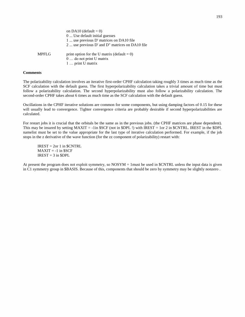
193

on DA10 (default = 0)

0 ... Use default initial guesses

1 ... use previous D' matrices on DA10 file

2 ... use previous D' and D" matrices on DA10 file

MPFLG print option for the U matrix (default = 0)

0 … do not print U matrix

1 … print U matrix

Comments

The polarizability calculation involves an iterative first-order CPHF calculation taking roughly 3 times as much time as the

SCF calculation with the default guess. The first hyperpolarizability calculation takes a trivial amount of time but must

follow a polarizability calculation. The second hyperpolarizability must also follow a polarizability calculation. The

second-order CPHF takes about 6 times as much time as the SCF calculation with the default guess.

Oscillations in the CPHF iterative solutions are common for some components, but using damping factors of 0.15 for these

will usually lead to convergence. Tighter convergence criteria are probably desirable if second hyperpolarizabilities are

calculated.

For restart jobs it is crucial that the orbitals be the same as in the previous jobs. (the CPHF matrices are phase dependent).

This may be insured by setting MAXIT = -1in $SCF (not in $DPL !) with IREST = 1or 2 in $CNTRL. IREST in the $DPL

namelist must be set to the value appropriate for the last type of iterative calculation performed. For example, if the job

stops in the z derivative of the wave function (for the zz component of polarizability) restart with:

IREST = 2or 1 in $CNTRL

MAXIT = -1 in $SCF

IREST = 3 in $DPL

At present the program does not exploit symmetry, so NOSYM = 1must be used in $CNTRL unless the input data is given

in C1 symmetry group in $BASIS. Because of this, components that should be zero by symmetry may be slightly nonzero .

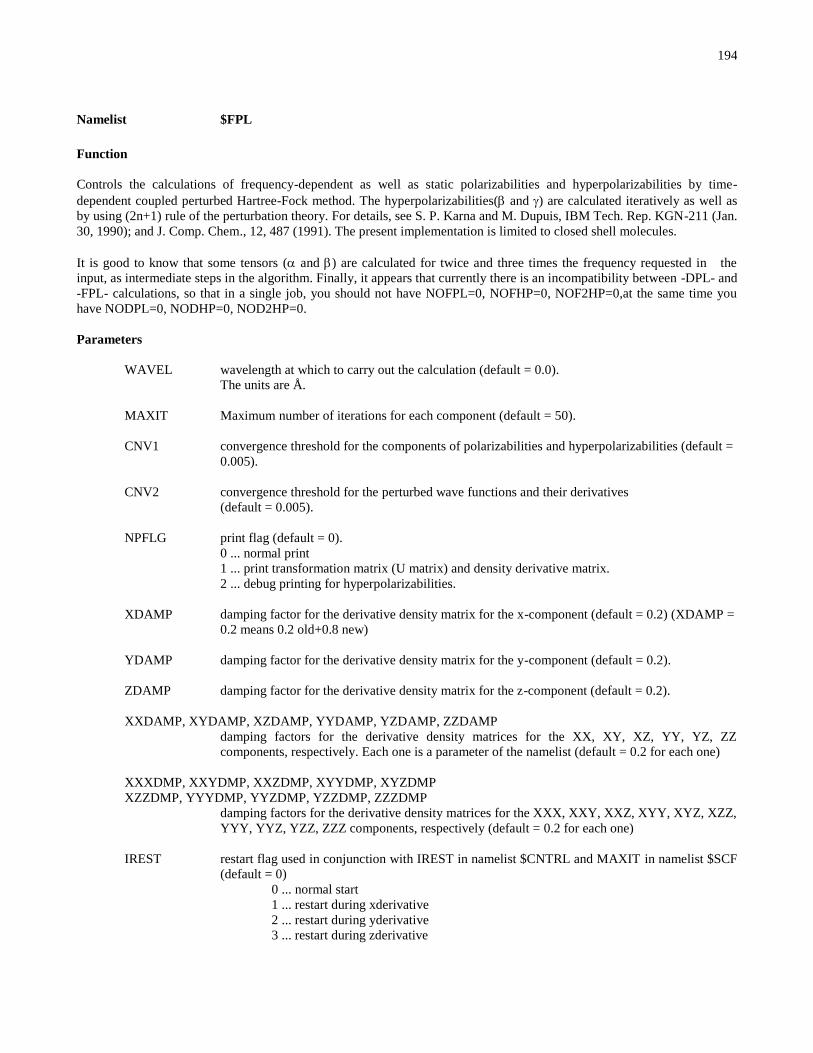
194

Namelist $FPL

Function

Controls the calculations of frequency-dependent as well as static polarizabilities and hyperpolarizabilities by time-

dependent coupled perturbed Hartree-Fock method. The hyperpolarizabilities( and ) are calculated iteratively as well as

by using (2n+1) rule of the perturbation theory. For details, see S. P. Karna and M. Dupuis, IBM Tech. Rep. KGN-211 (Jan.

30, 1990); and J. Comp. Chem., 12, 487 (1991). The present implementation is limited to closed shell molecules.

It is good to know that some tensors ( and ) are calculated for twice and three times the frequency requested in the

input, as intermediate steps in the algorithm. Finally, it appears that currently there is an incompatibility between -DPL- and

-FPL- calculations, so that in a single job, you should not have NOFPL=0, NOFHP=0, NOF2HP=0,at the same time you

have NODPL=0, NODHP=0, NOD2HP=0.

Parameters

WAVEL wavelength at which to carry out the calculation (default = 0.0).

The units are Å.

MAXIT Maximum number of iterations for each component (default = 50).

CNV1 convergence threshold for the components of polarizabilities and hyperpolarizabilities (default =

0.005).

CNV2 convergence threshold for the perturbed wave functions and their derivatives

(default = 0.005).

NPFLG print flag (default = 0).

0 ... normal print

1 ... print transformation matrix (U matrix) and density derivative matrix.

2 ... debug printing for hyperpolarizabilities.

XDAMP damping factor for the derivative density matrix for the x-component (default = 0.2) (XDAMP =

0.2 means 0.2 old+0.8 new)

YDAMP damping factor for the derivative density matrix for the y-component (default = 0.2).

ZDAMP damping factor for the derivative density matrix for the z-component (default = 0.2).

XXDAMP, XYDAMP, XZDAMP, YYDAMP, YZDAMP, ZZDAMP

damping factors for the derivative density matrices for the XX, XY, XZ, YY, YZ, ZZ

components, respectively. Each one is a parameter of the namelist (default = 0.2 for each one)

XXXDMP, XXYDMP, XXZDMP, XYYDMP, XYZDMP

XZZDMP, YYYDMP, YYZDMP, YZZDMP, ZZZDMP

damping factors for the derivative density matrices for the XXX, XXY, XXZ, XYY, XYZ, XZZ,

YYY, YYZ, YZZ, ZZZ components, respectively (default = 0.2 for each one)

IREST restart flag used in conjunction with IREST in namelist $CNTRL and MAXIT in namelist $SCF

(default = 0)

0 ... normal start

1 ... restart during xderivative

2 ... restart during yderivative

3 ... restart during zderivative

195

4 ... restart during xxderivative

5 ... restart during xyderivative

6 ... restart during xzderivative

7 ... restart during yyderivative

8 ... restart during yzderivative

9 ... restart during zzderivative

10 ... restart during xxx derivative

11 ... restart during xxy derivative

12 ... restart during xxz derivative

13 ... restart during xyy derivative

14 ... restart during xyz derivative

15 ... restart during xzz derivative

16 ... restart during yyy derivative

17 ... restart during yyz derivative

18 ... restart during yzz derivative

19 ... restart during zzz derivative

IREST1 restart flag used in conjunction with IREST in this namelist (see above). This flag indicates at

which frequency combination the program restarts (default = 0). Note that the IREST, IREST1

pair is printed on the output listing of the first part of the calculation. IGUESS initial guess

density derivative matrix (default = 0)

0 ...default initial guess

1 ...use previous D' matrices on DA10 file.

2 ...use previous D' and D'' matrices on DA10 file

NOSTPL flag to calculate static polarizability (default = 0).

0 ... calculate (0)

1 ... skip.

NOFPL1 flag to calculate dynamic polarizability (default = 0).

()

1 ... skip.

NOFPL2 lag to calculate first order matrices for 2, needed for (SHG) and (EFISHG) (default = 0).

0 ... calculate

1 ... skip.

NOFPL3 flag to calculate first order matrices for 3, needed for (THG) (default = 0).

0 ... calculate

1 ... skip.

NOHPNI flag to calculate by (2n+1) rule (default = 0).

0 ... calculate.

1 ... skip.

NOHPI flag for iterative calculation of and second order wave functions and derivative matrices

(default = 0).

0 ... calculate .

1 ... skip.

NOSTHP flag to calculate (0,0) (default =0).

0 ... calculate.

1 ... skip.

NOEOPE flag to calculate (0, ) (default = 0).

196

0 ... calculate.

1 ... skip.

NOSHG flag to calculate ( , ) (default = 0)

0 ... calculate.

1 ... skip.

NOOR flag to calculate ( , - ) (default = 0)

0 ... calculate.

1 ... skip.

NO2HNI flag to calculate by (2n+1) rule (default = 0).

0 ... calculate.

1 ... skip.

NO2HI flag to calculate iteratively (default = 1).

0 ... calculate.

1 ... skip.

NOST2H flag to calculate (0,0,0,) (default = 0).

0 ... calculate.

1 ... skip.

NOOKE flag to calculate (0,0, ) (default = 0).

0 ... calculate.

1 ... skip.

NOEFSH flag to calculate (0, , ) (default = 0).

0 ... calculate.

1 ... skip.

NOTHG flag to calculate ( , , ) (default = 0)

0 ... calculate.

1 ... skip.

NOIDRI flag to calculate ( , , - ) (default = 0).

0 ... calculate.

1 ... skip.

NOEFOR flag to calculate (0, , - ) (default = 0).

0 ... calculate.

1 ... skip.

IGUESS set this parameter to 1 or 2 if the initial guess density derivative matrix is available

on DA10 (default = 0)

0 ... Use default initial guesses

1 ... use previous D' matrices on DA10 file

2 ... use previous D' , D" , and D’’’ matrices on DA10 file

197

Namelist $SOS

Function

Controls the calculation of polarizabilities and hyperpolarizabilities via the sum-over-states method of Fripiat et al.:

J.G.Fripiat, C.Barbier, V.P.Bodart, and J.M.Andre, J.Comp.Chem. 7, 756 (1986).

Parameters

NCORB number of orbitals treated as core, not included in the SOS sum (default = 0)

NORB total number of orbitals included in the SOS sum (default = all orbitals).

Comments

This method corresponds to the un-coupled Hartree-Fock method. We do not have much experience with regards to how it

performs compared to the CPHF approach described below.

198

Namelist $BOYS

Function

This namelist controls the localization of molecular orbitals via Boys' method.

Parameters

NORB number of orbitals to be localized using Boys' method

IFRZ(512) serial number of the orbitals to be kept unchanged (frozen) during the localization procedure

(default = 512*0).

IPAIR(512) serial number of orbitals for which a correlating orbital need be generated. For example the

correlating orbital of a bonding orbital is the antibonding * orbital. This step works for bond

orbitals only, not lone pair orbitals. Note that the orbitals are left in the same order as the initial

orbitals. The frozen orbitals are at the same place. The correlating orbitals are appended to the

initial set.

Comments

It is not unusual to see the localization procedure not converge. In many cases this lack of convergence may be related to

orbitals that describe lone pairs of electrons. Also core electrons may create problems. A step by step approach in which

orbitals of this nature are omitted from the list of orbitals to be localized will often lead to the desired localization.

Another prototypical example would be the localization of molecular orbitals in the ethylene molecule C2H4. When all the

orbitals are included in the localization process, two 'banana' bonds are generated from the CC and orbitals. To obtain a

true CC bond it is necessary to freeze the orbital.

199

Data group $STONE

Function

This data group defines the expansion points for Stone's distributed multipole analysis. Points may be defined at atom

centers, bond midpoints, bond overlap centers of charge, molecular center of mass, or any other user defined point. The

several types of input lines (format-free) are described below. Enter as many lines as you wish, terminated by a line with

$END. The distributed multipole method takes the multipolar expansion of each overlap charge density defined by two

gaussian primitives, and translates it from the center of charge of the overlap density to the nearest expansion point.

A map of the electrostatic potential due to the multipole expansion is calculated. It suffices to specify the 3D-grid, by

means of the $MAP namelist input.

This code is adapted from the work of W.Stevens and collaborators.

Finally note that the input specification must use UPPER CASE characters.

Cards

ATOM i <name>

'atom' a keyword indicating that an atom is selected as an expansion center. i the

number of the atom, corresponding to an atom in the $BASIS input. <name> an

optional name for the atom. If not entered the name will be set to the name used in the

$BASIS input.

BOND i j <name>

'bond' keyword indicating that a bond midpoint is selected as an expansion center. i,j

the indices of the atoms defining the bond, corresponding to two atoms in the $BASIS

input. <name> an optional name for the bond midpoint. If not entered the name will be

set to 'bond'.

OLAP i j <name>

'olap' keyword indicating that the center of charge of a bond overlap distribution is

selected as an expansion center. i,j the indices of the atoms defining the bond,

corresponding to two atom in the $BASIS input. <name> an optional name for the

overlap expansion point. If omitted, it will be set to 'olap'.

POINT x y z <name>

'point' keyword indicating that a user defined point is selected as an expansion point.

x,y,z are the coordinates of the point (in a.u.). <name> an optional name for the point.

If omitted, it will be set to 'point'

CMASS

a line with 'cmass' as the keyword will select the center of mass of the molecule as an

expansion point.no other input on the line is necessary.

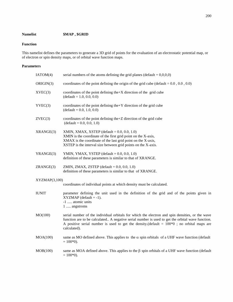
200

Namelist $MAP , $GRID

Function

This namelist defines the parameters to generate a 3D grid of points for the evaluation of an electrostatic potential map, or

of electron or spin density maps, or of orbital wave function maps.

Parameters

IATOM(4) serial numbers of the atoms defining the grid planes (default = 0,0,0,0)

ORIGIN(3) coordinates of the point defining the origin of the grid cube (default = 0.0 , 0.0 , 0.0)

XVEC(3) coordinates of the point defining the+X direction of the grid cube

(default = 1.0, 0.0, 0.0)

YVEC(3) coordinates of the point defining the+Y direction of the grid cube

(default = 0.0, 1.0, 0.0)

ZVEC(3) coordinates of the point defining the+Z direction of the grid cube

(default = 0.0, 0.0, 1.0)

XRANGE(3) XMIN, XMAX, XSTEP (default = 0.0, 0.0, 1.0)

XMIN is the coordinate of the first grid point on the X-axis,

XMAX is the coordinate of the last grid point on the X-axis,

XSTEP is the interval size between grid points on the X-axis.

YRANGE(3) YMIN, YMAX, YSTEP (default = 0.0, 0.0, 1.0)

definition of these parameters is similar to that of XRANGE.

ZRANGE(3) ZMIN, ZMAX, ZSTEP (default = 0.0, 0.0, 1.0)

definition of these parameters is similar to that of XRANGE.

XYZMAP(3,100)

coordinates of individual points at which density must be calculated.

IUNIT parameter defining the unit used in the definition of the grid and of the points given in

XYZMAP (default = -1).

-1 ..... atomic units

1 ..... angstroms

MO(100) serial number of the individual orbitals for which the electron and spin densities, or the wave

function are to be calculated.. A negative serial number is used to get the orbital wave function.

A positive serial number is used to get the density.(default = 100*0 ; no orbital maps are

calculated).

MOA(100) same as MO defined above. This applies to the spin orbitals of a UHF wave function (default

= 100*0).

MOB(100) same as MOA defined above. This applies to the spin orbitals of a UHF wave function (default

= 100*0).

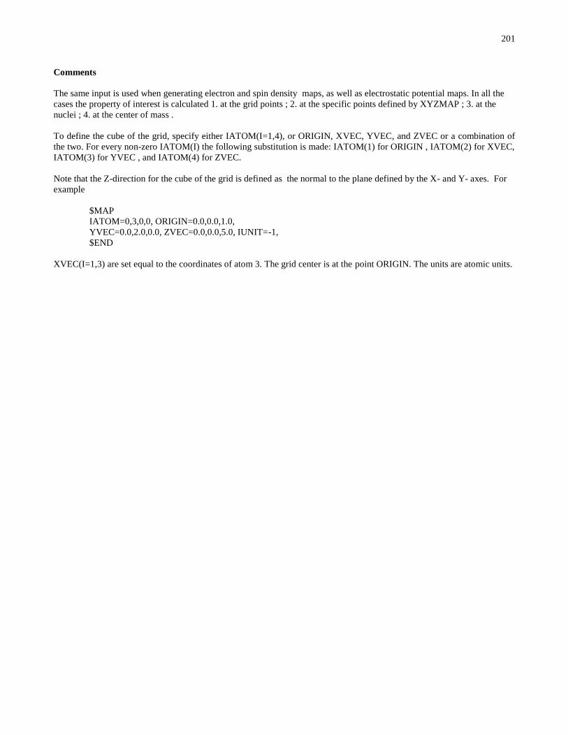
201

Comments

The same input is used when generating electron and spin density maps, as well as electrostatic potential maps. In all the

cases the property of interest is calculated 1. at the grid points ; 2. at the specific points defined by XYZMAP ; 3. at the

nuclei ; 4. at the center of mass .

To define the cube of the grid, specify either IATOM(I=1,4), or ORIGIN, XVEC, YVEC, and ZVEC or a combination of

the two. For every non-zero IATOM(I) the following substitution is made: IATOM(1) for ORIGIN , IATOM(2) for XVEC,

IATOM(3) for YVEC , and IATOM(4) for ZVEC.

Note that the Z-direction for the cube of the grid is defined as the normal to the plane defined by the X- and Y- axes. For

example

$MAP

IATOM=0,3,0,0, ORIGIN=0.0,0.0,1.0,

YVEC=0.0,2.0,0.0, ZVEC=0.0,0.0,5.0, IUNIT=-1,

$END

XVEC(I=1,3) are set equal to the coordinates of atom 3. The grid center is at the point ORIGIN. The units are atomic units.

202

Namelist $FLD

Function

This namelist contains the information related to an uniform field applied on the molecule. Note that an uniform field

defined with the present namelist and a non-uniform field defined by means of point charges (see data group $EFC) may

not be applied at the same time.

Parameters

FLDX strength of field applied in the -X- direction (default = 0.0 a.u.).

FLDY strength of field applied in the -Y- direction (default = 0.0 a.u.).

FLDZ strength of field applied in the -Z- direction (default = 0.0 a.u.).

Comments

Because of the uniform field the electronic density may no longer have the symmetry of the molecular frame. This implies

that one must use a lower symmetry point group or turn off symmetry, by setting NOSYM = 1 in $CNTRL .

The input parameters defined above may have positive and negative values. They define the magnitude and the direction of

the field.

203

Data group $QREL

Function

The presence of this data group results in including one-electron Darwin and mass-velocity terms treated self-consistently.

His code originates from Dr. T. Nakajima and Prof. K. Hirao of the University of Tokyo.

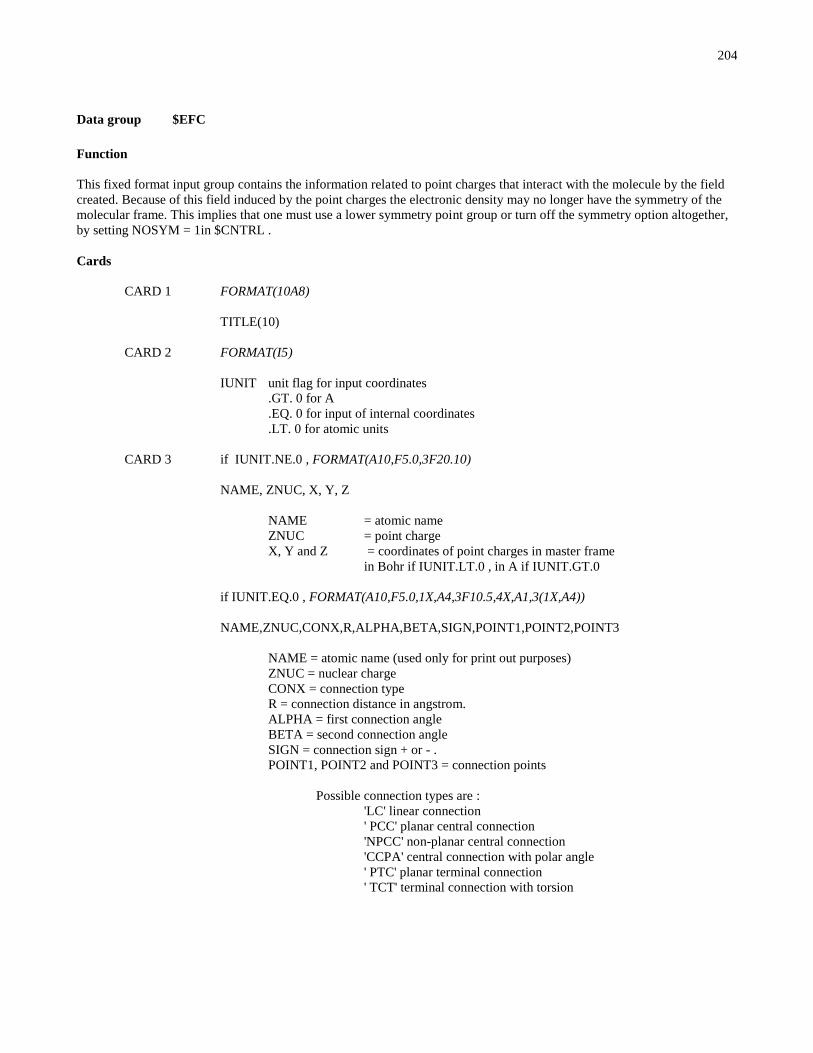
204

Data group $EFC

Function

This fixed format input group contains the information related to point charges that interact with the molecule by the field

created. Because of this field induced by the point charges the electronic density may no longer have the symmetry of the

molecular frame. This implies that one must use a lower symmetry point group or turn off the symmetry option altogether,

by setting NOSYM = 1in $CNTRL .

Cards

CARD 1 FORMAT(10A8)

TITLE(10)

CARD 2 FORMAT(I5)

IUNIT unit flag for input coordinates

.GT. 0 for A

.EQ. 0 for input of internal coordinates

.LT. 0 for atomic units

CARD 3 if IUNIT.NE.0 , FORMAT(A10,F5.0,3F20.10)

NAME, ZNUC, X, Y, Z

NAME = atomic name

ZNUC = point charge

X, Y and Z = coordinates of point charges in master frame

in Bohr if IUNIT.LT.0 , in A if IUNIT.GT.0

if IUNIT.EQ.0 , FORMAT(A10,F5.0,1X,A4,3F10.5,4X,A1,3(1X,A4))

NAME,ZNUC,CONX,R,ALPHA,BETA,SIGN,POINT1,POINT2,POINT3

NAME = atomic name (used only for print out purposes)

ZNUC = nuclear charge

CONX = connection type

R = connection distance in angstrom.

ALPHA = first connection angle

BETA = second connection angle

SIGN = connection sign + or - .

POINT1, POINT2 and POINT3 = connection points

Possible connection types are :

'LC' linear connection

' PCC' planar central connection

'NPCC' non-planar central connection

'CCPA' central connection with polar angle

' PTC' planar terminal connection

' TCT' terminal connection with torsion

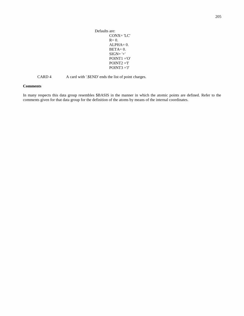
205

Defaults are:

CONX= 'LC'

R= 0.

ALPHA= 0.

BETA= 0.

SIGN= '+'

POINT1 ='O'

POINT2 ='I'

POINT3 ='J'

CARD 4 A card with '.$END' ends the list of point charges.

Comments

In many respects this data group resembles $BASIS in the manner in which the atomic points are defined. Refer to the

comments given for that data group for the definition of the atoms by means of the internal coordinates.

206

Namelist $EFC2

Function

This namelist is used when the input for effective charges is given in an alternate unix file, rather than in the data group

$EFC as described above.

Parameters

EFCFIL unix name of the alternate file containing the input data for the effective charges.

Comments

The format of the EFCFIL file is: sequential, unformatted. The first record is a character*80 record title, each subsequent

record, also unformatted, include a character*8 label, the effective charge, and the three Cartesian coordinates.

207

Data group $QMMM

Function

The presence of this data group signals the code that this is a QM/MM system. The data group specifies the coordinates of

the water molecules. This is accomplished via the format .car of Biosym. The Lennard-Jones parameters assigned to the

QM subsystem are given with the namelist $QM, the charges and Lennard-Jones parameters of the MM subsystem are

given with the $MM or $MMPOL namelists. See below.

Parameters

A complete .car input. Follows the keyword $QMMM

1. BIOSYM '!BIOSYM archive 3'

FORMAT(A17)

2. BIOPBC 'PBC=OFF'

FORMAT(A7)

3. TITLE '!DATE'

FORMAT(A80)

4. BIODAT

FORMAT(A5)

5. atom_name , atom_x , atom_y , atom_z , atom_residue , biopar , atom_symbol , atom_charge

FORMAT(A5,3F15.9,1X,A12,A2,6X,A2,1X,F6.3)

one line 5. for each atom.

6. BIOEND 'end '

FORMAT(A5)

7. BIOEND 'end '

FORMAT(A5)

Comments

DATA BIOSYM /'!BIOSYM archive 3'/

DATA BIOPBC /'PBC=OFF'/

DATA BIORES /'HND_ 1h '/

DATA BIODAT /'!DATE'/

DATA BIOPAR /'? '/

DATA BIOEND /'end '/

If the $QMMM data group is used with the $QM namelist, the $QM namelist must always occur before the $QMMM data

group in the input file.

208

Namelist $QM

Function

This namelist defines the Lennard-Jones parameters for the QM subsystem of a QM/MM system.

Parameters

QSEQM(3,128) q, , and parameters for the QM subsystem. Note that the q's are not used, since they

are replaced by the QM electronic charge distribution. and are the usual Lennard-

Jones parameters, for example as defined in the OPLS force field.

QSEQM(1,IAT) = q for quantum atom IAT

QSEQM(2,IAT) = for atom IAT

QSEQM(3,IAT) = for atom IAT

Comments

If both the $QM namelist and the $QMMM data group are used, the $QM namelist must always occur before the $QMMM

data group.

209

Namelist $MMNOPOL

Function

This namelist defines the molecular mechanics parameters of the MM subsystem of a QM/MM system.

Parameters

QSEMM(3, 3*73) q, , and parameters for the MM subsystem. The parameters are of the type found in

the TIP3P, or POL1, or POL2 potential parameters.

QSEMM(1,IEF) = q for mm atom IEF

QSEMM(2,IEF) = for mm atom IEF


Comments

In previous versions of HONDO, this namelist was referred to as $MM. The name has been changed to avoid conflicts

with the $MMPOL namelist (see AIX, IRIX, and Linux implementations for further details).

210

Namelist $MMPOL

Function

Parameters

QSEMM(3, 3*73) q, , and parameters for the MM subsystem. The parameters are of the type found in

the TIP3P, or POL1, or POL2 potential parameters.

QSEMM(1,IEF) = q for mm atom IEF



ALFMM(3*73) isotropic atomic polarizability for MM atom IEF, such as those defined in POL1 and

POL2.

Comments

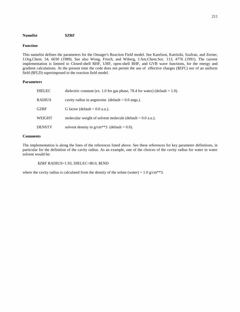
211

Namelist $ZRF

Function

This namelist defines the parameters for the Onsager's Reaction Field model. See Karelson, Katritzki, Szafran, and Zerner,

J.Org.Chem. 54, 6030 (1989). See also Wong, Frisch, and Wiberg, J.Am.Chem.Soc. 113, 4776 (1991). The current

implementation is limited to Closed-shell RHF, UHF, open-shell RHF, and GVB wave functions, for the energy and

gradient calculations. At the present time the code does not permit the use of effective charges ($EFC) nor of an uniform

field ($FLD) superimposed to the reaction field model.

Parameters

DIELEC dielectric constant (ex. 1.0 for gas phase, 78.4 for water) (default = 1.0).

RADIUS cavity radius in angstroms (default = 0.0 angs.).

GZRF G factor (default = 0.0 a.u.).

WEIGHT molecular weight of solvent molecule (default = 0.0 a.u.).

DENSTY solvent density in g/cm**3 (default = 0.0).

Comments

The implementation is along the lines of the references listed above. See these references for key parameter definitions, in

particular for the definition of the cavity radius. As an example, one of the choices of the cavity radius for water in water

solvent would be:

$ZRF RADIUS=1.93, DIELEC=80.0, $END

where the cavity radius is calculated from the density of the solute (water) = 1.0 g/cm**3.

212

Namelists $HONDOS, $CM2, and $SM5

Function

These namelists define the parameters for a calculation of CM2, CM3, or CM4 charges, evaluation of the free energy of

solvation in a given solvent using the SMx (x = 5.42, 5.43, and 6) model, and for a calculation of the electrostatic

contribution to the free energy of solvation using the generalized Born (GB) model. Only one namelist should be used for a

particular calculation. If more than one namelist is provided in the input file, all but the first encountered in the input will

be ignored by the program.

Parameters

ISCRF Controls the type of SCF to be performed:

ISCRF = 0 invokes the gas-phase calculation of Löwdin and/or RLPA charges and CM2, CM3, or CM4 charges

(default)

ISCRF = 1 invokes the gas- and liquid-phase calculation of Löwdin and/or RLPA charges and CM2, CM3, or

CM4 charges and the calculation of solvation free energy using SCF Scheme I (see the section entitled SCF

Schemes)

ISCRF = 2 invokes the gas- and liquid-phase calculation of Löwdin and/or RLPA charges and CM2, CM3, or

CM4 charges and the calculation of solvation free energy using SCF Scheme II (see the section entitled SCF

Schemes)

ISCRF = 3 uses user-supplied partial atomic charges (see the ICRead option below) in the evaluation of solvation

free energy using SCF Scheme III (see the section entitled SCF Schemes)

Note that when RLPA charges are calculated and printed, so are Löwdin charges. However, for liquid-phase calculations

that use RLPA charges, the Löwdin charges correspond to the converged SCRF achieved with RLPA charges, not with

Löwdin charges. Also note RLPA charges should only be calculated by methods that use the 6-31+G* or 6-31+G** basis

set, while Löwdin charges should be used for other methods.

ICMD Selects the set of CM2, CM3, or CM4 coefficients used for the evaluation of the CM2, CM3, or CM4

charges. By default, ICMD is set equal to 1. The table below matches the value of ICMD with the wave

function for which the corresponding CM2, CM3, or CM4 parameter set has been optimized. The use of

Löwdin atomic charges in the evaluation of the free energy of solvation is requested by setting ICMD

equal to zero. A value of 300 for ICMD is used to request the use of RLPA charges in the evaluation of

the free energy of solvation. For ICMD values of 314, 318, 319, 418, and 419 RLPA charges, not

Löwdin charges, are mapped to CM3 or CM4 charges.

ICDS ICMD Wave function which corresponds to set of coefficients

0 0 All coefficients equal zero, calculate Löwdin charges

1 1 CM2/HF/MIDI! (default for ICMD)

2 2 CM2/HF/MIDI!6D

3 3 CM2/HF/6-31G*

4 4 CM2/BPW91/MIDI!

5 5 CM2/BPW91/MIDI!6D

6 6 CM2/B3LYP/MIDI!

7 7 CM2/BPW91/6-31G*

8 8 CM2/HF/6-31+G*

9 9 CM2/HF/cc-pVDZ

10 10 CM2/HF/MIDI!6D

0 301 CM3/HF/MIDI!

0 302 CM3/HF/MIDI!6D

303 303 CM3/HF/6-31G*

313 313 CM3/B3LYP/6-31G*

213

0 314 CM3/B3LYP/6-31+G*

315 315 CM3/MPWX/MIDI!

316 316 CM3/MPWX/MIDI!6D

317 317 CM3/MPWX/6-31G*

318 318 CM3/MPWX/6-31+G*, uses RLPA charges

319 319 CM3/MPWX/6-31+G**, uses RLPA charges

0 320 CM3/B3LYP/MIDI!6D

0 321 CM3/BLYP/6-31G*

0 322 CM3.1/HF/MIDI!

416 416 CM4/DFT/MIDI!6D

417 417 CM4/DFT/6-31G*

418 418 CM4/DFT/6-31+G*, uses RLPA charges

419 419 CM4/DFT/6-31+G**, uses RLPA charges

0 300 Calculate RLPA charges

In the above table, X corresponds to the percentage of Hartree-Fock exchange used in the mPW hybrid density functional

(see the HFE keyword for more details). For SM6, DFT refers to any good density functional. A list of recommended

density functionals that are supported in HONDOPLUS is given in the section entitled “Density Functional Methods

Recommended for use with CM4 and SM6 in HONDOPLUS”. In cases where the default value of ICDS = 0, a solvation

model does not exist for that particular set of charges. For ICMD = 300, all restricted and unrestricted HF, DFT, and hybrid

DFT methods are available, but only the 6-31+G* or the 6-31+G** basis set should be used. Note that CM3 for the BLYP

and B3LYP methods and CM3.1 for the HF/MIDI! method in the above table uses a different mapping function for

compounds that contain N and O than CM3 for MPWX and HF does. For more information, see “Parameterization of

Charge Model 3 For AM1, PM3, BLYP, and B3LYP” by Thompson, J. D.; Cramer, C. J.; Truhlar, D. G. J. Comput. Chem.,

2003, 24, 1291 and “Accurate Partial Atomic Charges for High-Energy Molecules with the MIDI! Basis Set” by Kelly, C.

P.; Cramer, C. J; Truhlar, D. G. Theor. Chem. Acc. 2005, 113, 133.

ICDS Selects the set of coefficients that will be used to evaluate the atomic surface tensions. The table above

matches the value of ICDS with the wave function for which the corresponding CDS parameter set has

been optimized. A generalized Born model limited to electrostatics only is invoked by setting ISCRF

greater than 0 and by setting ICDS = 0. In a SM5.42, SM5.43, or SM6 calculation, by default, the value

used for ICDS is set equal to the value specified for ICMD. Thus, for most calculations, the only the

ICMD keyword (described below) needs to be specified in the input section. To set ICDS to a value that

is not equal to the value of ICMD implies that either or both the CMx coefficients and/or the surface

tension coefficients do not correspond to the wave function that is being employed, and as such the

results will not be consistent with any previously defined model. For allowed values of ICMD for which

a solvation model does not exist, the default is that ICDS is set equal to zero. Note that ICDS can be set

to zero for any value of ICMD.

HFE Defines the fraction of Hartree-Fock (HF) exchange to be used when ICMD = 315 to ICMD = 319 and

ICMD = 416 to ICMD = 419. For example, if a calculation of CM3 charges by the mPW1PW91/MIDI!

method were to be carried out, then ICMD would be set to 315, and HFE would be set to 0.25. The HFE

keyword only defines the fraction of HF exchange for a given calculation within the charge and solvation

model part of the program, not in the entire HONDOPLUS program. The fraction of HF exchange is

defined in the entire program through the DFTFUN keyword in the $SCF namelist. For example, if a

calculation of CM3 charges were to be carried out by the MPW40.0/6-31+G** method, then ICMD

would be set to 319 and HFE would be set to 0.40 in either the $HONDOS namelist, the $CM2 namelist

or the $SM5 namelist, and DFTFUN would have to be set equal to 3400 in the $SCF namelist. This

keyword is only active when ICMD = 315 – 319, and in these instances HFE must be explicitly specified

by the user in one of the three namelists. If ICMD = 315 – 319 or ICMD = 416 – 419 and HFE is not

defined by the user, HONDOPLUS will terminate.

IAQU (default = 1)

0 ..... Organic solvent

1 ..... Aqueous solution

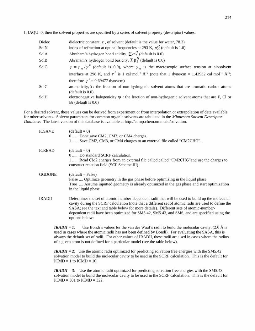
214

If IAQU=0, then the solvent properties are specified by a series of solvent property (descriptor) values:

Dielec dielectric constant, , of solvent (default is the value for water, 78.3)

SolN index of refraction at optical frequencies at 293 K, n20D

(default is 1.0)

SolA Abraham’s hydrogen bond acidity, 2H

(default is 0.0)

SolB Abraham’s hydrogen bond basicity, 2H

(default is 0.0)

SolG m /o

(default is 0.0), where m is the macroscopic surface tension at air/solvent

interface at 298 K, and o

is 1 cal·mol–1

Å–2

(note that 1 dyne/cm = 1.43932 cal·mol–1

Å–2

;

therefore o

= 0.69477 dyne/cm)

SolC aromaticity, : the fraction of non-hydrogenic solvent atoms that are aromatic carbon atoms

(default is 0.0)

SolH electronegative halogenicity, : the fraction of non-hydrogenic solvent atoms that are F, Cl or

Br (default is 0.0)

For a desired solvent, these values can be derived from experiment or from interpolation or extrapolation of data available

for other solvents. Solvent parameters for common organic solvents are tabulated in the Minnesota Solvent Descriptor

Database. The latest version of this database is available at http://comp.chem.umn.edu/solvation.

ICSAVE (default = 0)

0 ..... Don't save CM2, CM3, or CM4 charges.

1 ..... Save CM2, CM3, or CM4 charges to an external file called “CM2CHG”.

ICREAD (default = 0)

0 ..... Do standard SCRF calculation.

1 ..... Read CM2 charges from an external file called called “CM2CHG”and use the charges to

construct reaction field (SCF Scheme III).

GGDONE (default = False)

False .... Optimize geometry in the gas phase before optimizing in the liquid phase

True .... Assume inputted geometry is already optimized in the gas phase and start optimization

in the liquid phase

IRADII Determines the set of atomic-number-dependent radii that will be used to build up the molecular

cavity during the SCRF calculation (note that a different set of atomic radii are used to define the

SASA; see the text and table below for more details). Different sets of atomic-number-

dependent radii have been optimized for SM5.42, SM5.43, and SM6, and are specified using the

options below:

IRADII = 1: Use Bondi’s values for the van der Waal’s radii to build the molecular cavity, (2.0 Å is

used in cases where the atomic radii has not been defined by Bondi). For evaluating the SASA, this is

always the default set of radii. For other values of IRADII, these radii are used in cases where the radius

of a given atom is not defined for a particular model (see the table below).

IRADII = 2: Use the atomic radii optimized for predicting solvation free energies with the SM5.42

solvation model to build the molecular cavity to be used in the SCRF calculation. This is the default for

ICMD = 1 to ICMD = 10.

IRADII = 3: Use the atomic radii optimized for predicting solvation free energies with the SM5.43


ICMD = 301 to ICMD = 322.

215

IRADII = 4: Use the atomic radii optimized for predicting solvation free energies with the SM6


ICMD = 0, ICMD = 300, and ICMD = 416 to ICMD = 419.

The four sets of radii described above are listed below. In cases where the atomic radius of a given atom is not defined, the

default value is Bondi’s radii. For elements whose atomic radii are not listed in Bondi’s paper, a value of 2.0 Å is used for

the radius. Thus, Generalized Born calculations may be carried out for a molecule containing any element on the periodic

table.

Elementa IRADII = 1b IRADII = 2c,d IRADII = 3c,e IRADII = 4c,f

H 1.20 0.91 0.79 1.02

Li 1.82 1.32 — —

C 1.70 1.78 1.81 1.57

N 1.55 1.92 1.66 1.61

O 1.52 1.60 1.63 1.52

F 1.47 1.50 1.58 1.47

Ne 1.54 — — —

Na 2.27 — — —

Mg 1.73 — — —

Al 2.50 — — —

Si 2.10 — — —

P 1.80 2.27 2.01 1.80

S 1.80 1.98 2.22 2.12

Cl 1.75 2.13 2.28 2.02

Ar 1.88 — — —

K 2.75 — — —

Ni 1.63 — — —

Cu 1.40 — — —

Zn 1.39 — — —

Ga 2.40 — — —

Ge 2.10 — — —

As 1.85 — — —

Se 1.90 — — —

Br 1.85 2.31 2.38 2.60

Kr 2.02 — — —

Pd 1.63 — — —

Ag 1.72 — — —

Cd 1.58 — — —

In 2.50 — — —

Sn 2.20 — — —

Sb 2.10 — — —

Te 2.06 — — —

I 1.98 2.66 — —

Xe 2.60 — — —

aFor atoms not listed in this table, a radius of 2.0 Å is used. bBondi’s values for the van der Waals radius (Bondi, A.

J. Phys. Chem. 1964, 68, 441). cIn cases where the atomic radius is not defined, Bondi’s values are used. In cases

where the atomic radius has not been defined by Bondi, 2.0 Å is used for the atomic radius. dThese radii have been

optimized for use with the SM5.42 model. eThese radii have been optimized for use with the SM5.43 model. fThese

radii have been optimized for use with the SM6 model.

216

ISTS Determines whether the SM5 (ISTS = 5) or SM6 (ISTS = 6) functional forms will be used in evaluating

GCDS. For all values of ICMD between 0 and 322, the default value is ISTS =5. For all values of

ICMD between 416 and 419, the default value is ISTS = 6.

SolvRd Value of the solvent radius (in angstroms) for the calculation of the solvent-accessible surface areas of the

atoms of the solute (default 0.40 Å). For predicting solvation free energies with SM5.42, SolvRd should

be set to 0 Å. For predicting solvation free energies with SM5.43 or SM6, the default value of 0.40 Å

should be used.

SolK The temperature at which the solute free energy of solvation is computed in aqueous solution. The current

model is only applicable to H, C and O containing compounds for the range of temperatures in which

water is liquid (273 to 373 K). Note the model uses a temperature-dependent dielectric constant, the

equation for it was obtained from the CRC Handbook of Chemistry and Physics 76th

edition, ed. Lide, D.

R., 1995, CRC Press, New York. The default value is 298 K.

ReadK When .TRUE., this variable causes HONDOPLUS to read in a list of temperatures at which to compute

free energies of solvation from a file labeled “Temperatures.” The first line in the input file must list the

number of temperatures at which the free energy of solvation is to be computed. Then each succeeding

line should list only one temperature. This method uses the converged wavefunction at each temperature

as a starting guess for the succeeding temperature. This approach saves some time by avoiding the need

to recompute the gas phase structure of the solute, however if the temperatures are closely spaced, the

perturbation introduced by the new temperature may not be greater than the convergence criteria. This is

not particularly problematic save that a electronic energies computed in this fashion will differ slightly

from those obtained by computing each temperature individually using SolK. This problem can be

avoided by using very tight convergence criteria; however the increase in time due to the tighter criteria

counterbalances the time savings from computing the gas-phase electronic structure of the solute only

once. This approach should only be used with temperatures that are more than 20 K apart. The default for

this option is .FALSE.. (NOTE: some compilers will not correctly read in input if the logicals in the input

do not have periods on either side of the value, ie ReadK=TRUE may cause problems whereas

ReadK=.True. or ReadK=.T. should not)

AvgK This option is similar to ReadK however instead of computing the electronic energy of the solute in

solution at each temperature; it computes the electronic energy of the solute at the average temperature

and scales the electronic energy of the solute using the following factor

Avg

T

11

11

where Avg is the dielectric constant of water at the average temperature and T is the dielectric

constant of water at a given temperature, T. This corresponds assuming that the charge on the solute does

not change significantly as a function of temperature. This approach can compute a large number of

temperatures with nearly the same computation time as that of a single temperature. This approach does

deviate mildly from the individual computations performed at each temperature; however, the deviation is

minor.

Comments:

In versions later than and including 3.3, Löwdin, RLPA, CM2, CM3, CM4 partial atomic charges, SMx (x = 5.42,

5.43, and 6), and GB liquid-phase wave functions and free energies of solvation may be calculated with

restricted closed-shell and unrestricted HF, DFT, and hybrid DFT methods, but not with restricted open-

shelled methods (ROHF or ROB3LYP).

217

ICMD and ICDS should always be explicitly set to the value corresponding to the wave function used in the

calculation, otherwise a non-standard run will be performed. One way to accomplish this is to leave

ICDS blank. If that is done, the default is to set it equal to ICMD in cases for which a solvation model

exists, and zero when a solvation model for the value of ICMD does not exist.

Analytical gradients and geometry optimizations are available for all restricted and unrestricted wave functions

that employ Cartesian d functions (i.e., for ICMD = 0, 2, 3, 5, 7, 8, 10, 300, 302, 303, 313, 314, 316, 317,

318, 319, 320, 321, 416, 417, 418, and 419) and ISCRF = 1. Geometry optimization utilizing numerical

gradients are not yet available.

For geometry optimizations with the SMx (x = 5.42, 5.43, 6 and 6T) model, the program assumes that the input

geometry is the gas-phase optimum structure. HONDOPLUS uses this structure as the starting point for a

geometry optimization in solution.

When using wave functions that use spherical harmonic d and f functions (e.g., HF/MIDI!, BPW91/MIDI!,

B3LYP/MIDI!, HF/cc-pVDZ, and MPWX/MIDI!), ISPHER = 1 must be set in the $CNTRL namelist.

218

HONDOPLUS Keywords Required for Running Standard SMx Calculations

Shown in the below table are the HONDOPLUS keywords required for running standard SM5.42, SM5.43, and SM6

calculations. Note that the keywords entered in the $HONDOPLUS, $CM2, or $SM5 namelist are used by the solvation

and charge model portion of HONDOPLUS. Thus, keywords used by the rest of the HONDOPLUS program, such as the level

of theory, basis set, scf and geometry optimization options, etc., must also be included in the route section of the input file.

Method ISTS ICMD ICDS IRADII SolvRd HFE

SM5.42/HF/MIDI! a 5 1 1 2 0.00 N/A

SM5.42/HF/MIDI!6D 5 2 2 2 0.00 N/A

SM5.42/HF/6-31G* 5 3 3 2 0.00 N/A

SM5.42/HF/6-31+G* 5 8 8 2 0.00 N/A

SM5.42/HF/cc-pVDZ a 5 9 9 2 0.00 N/A

SM5.42/BPW91/MIDI! a 5 4 4 2 0.00 N/A

SM5.42/BPW91/MIDI!6D 5 5 5 2 0.00 N/A

SM5.42/BPW91/6-31G* 5 7 7 2 0.00 N/A

SM5.42/BPW91/DZVP 5 10 10 2 0.00 N/A

SM5.42/B3LYP/MIDI! a 5 6 6 2 0.00 N/A

SM5.43/HF/6-31G* 5 303 303 3 0.40 N/A

SM5.43/B3LYP/6-31G* 5 313 313 3 0.40 N/A

SM5.43/MPWX/MIDI! a 5 315 315 3 0.40 X

SM5.43/MPWX/MIDI!6D 5 316 316 3 0.40 X

SM5.43/MPWX/6-31G* 5 317 317 3 0.40 X

SM5.43/MPWX/6-31+G* 5 318 318 3 0.40 X

SM5.43/MPWX/6-31+G** 5 319 319 3 0.40 X

SM6/DFT/MIDI!6D 6 416 416 4 0.40 a

SM6/DFT/6-31G* 6 417 417 4 0.40 a SM6/DFT/6-31+G* 6 418 418 4 0.40 a SM6/DFT/6-31+G** 6 419 419 4 0.40 a

In the above table, X corresponds to the percentage of Hartree-Fock exchange used in the mPW hybrid density functional

(see the HFE keyword for more details). For SM6, DFT refers to any good density functional. A list of recommended

density functionals that are supported in HONDOPLUS is given in the section entitled “Density Functional Methods

Recommended for use with CM4 and SM6 in HONDOPLUS”. Also given in this section are the HFE values required by all of

the recommended density functionals.

aAnalytic gradients not available for this method.

bWhen using any of the CM4 or SM6 methods, the HFE keyword must always be specified (HFE = 0.00 should be entered

when using pure DFT functionals). For more details, see the section entitled “Density Functional Methods Recommended

for use with CM4 and SM6 in HONDOPLUS”.

219

Namelist $COSMO

Function

This namelist defines the parameters for the continuum solvent model COSMO.

Parameters

DIELEC dielectric constant (default = 0.0)

RSOLV radius of solvent probe

ISCREN charge renormalization option (default = 0)

0 ….

1 ….

MINBEM minimum level of sphere tesselation. The high tesselation level MAXBEM level gets reduced to

this level (default = 2).

MAXBEM maximum level of sphere tesselation (default = 4).

IFICOS flag to use an icosahedron as the starting structure for sphere tesselation (default = 0)

0 …. use octahedron as starting point

1 …. use icosahedron as starting point

RADIUS(128) atomic radii

LINEQ method for solving the linear equations to calculate the effective charges on the COSMO surface

(default = 0).

0 …. iterative method

1 …. dense linear equation solver

Comments

The code can handle the ‘united atom’ tesselation mode in which the hydrogen atoms are united to the atoms to which they

are linked.

220

Data group $ECP

Function

This data group, previously read in with a fixed format, and now read in with a free-format, contains the parameters for the

Effective Core Potential (ECP) approximation. A potential is read for each atom, starting at CARD 1. The ECP parameters

from Stevens, Basch and Krauss: W.J. Stevens, H. Basch, and M. Krauss, J.Chem.Phys. 81, 6026 (1984); W.J. Stevens, M.

Krauss, H. Basch, and P.G. Jasien, Can.J.Chem. (1992) are stored internally.

Other potentials for many atoms have been published . See for example: P.J. Hay and W.R. Wadt, J.Chem.Phys. 82, 299

(1985).

Cards

CARD 1 FORMAT(A8,I5,I5)

TYPE, IZCORE, LMAX

TYPE is a label for the ECP being read. For any tabulated potential, TYPE .eq.'CEP' is used to

retrieve the potential. If so, no further data is required.

IZCORE is the number of electrons included in the core and treated by the ECP .

LMAX is the highest angular momentum of the potential for this atom.

if TYPE .EQ. ' ', then no potential is used for this center. If TYPE is equal to a previous value

of TYPE, then the same potential is used for both centers and therefore in this case proceed back

to the next CARD 1.

CARD 2 FORMAT(I5)

NBF

NBF is the number of gaussian terms for the potential to follow.

CARD 3 FORMAT(F10.5,I5,F10.5)

COEF , N , ZETA

COEF is the coefficient for the gaussian term with radial dependence r**N, and exponent

ZETA. N is the exponent of r for the radial dependence of the gaussian term. ZETA is the

exponent of the gaussian term.

There are NBF cards (see CARD 2). The same type of input is needed for LMAX as defined on

CARD 1. Once the LMAX potential is read, then the lower potentials must follow with the

appropriate CARD 2 and the corresponding CARD 3.

When the potential on this center is complete, then go back to CARD 1.

221

Comments

ECP parameters for the first two rows are stored internally, and may be invoked by key words. An example of ECP for the

manganese hydride ion MnH+ follows:

$ECP

MN-ECP 10 2

1 -- MN -- L=2 POTENTIAL

-3.87049 1 15.92700

2 -- MN -- U(S-D) POTENTIAL

119.30400 2 10.78500

8.20795 0 64.76210

2 -- MN -- U(P-D) POTENTIAL

76.09500 2 10.39390

4.91435 0 54.71020

$END

Note that there must be a description of an ECP for every single atom. In the example above , the H atom does not have a

potential but a blank card is included in $ECP.

Another example for formamide NH2COH follows:

$ECP

O-ECP 2 1

1 ..... OXYGEN U(P).....

-0.92550 1 16.11718

2 ..... OXYGEN U(S-P) .....

1.96069 0 5.05348

29.13442 2 15.95333

C-ECP 2 1

1 ..... CARBON U(P).....

-0.89371 1 8.56468

2 ..... CARBON U(S-P) .....

1.92926 0 2.81497

14.88199 2 8.11296

N-ECP 2 1

1 ..... NITROGEN U(P).....

-0.91212 1 11.99686

2 ..... NITROGEN U(S-P) .....

1.93565 0 3.83895

21.73355 2 11.73247

$END

222

Namelist $CSOV

Function

This namelist is used to activate a CSOV calculation and specify the parameters of the interacting groups A and B. It must

be used in conjunction with appropriate $GUESS namelist and $VEC data groups. A detailed description of the algorithm

and relevant concepts can be found in: P.S.Bagus and F.Illas, J.Chem.Phys. 96, 8962 (1992).

Parameters

NOCO1 number of closed shell orbitals for fragment 1.

NOVI1 number of virtual orbitals for fragment 1.

NOCO2 number of closed shell orbitals for fragment 2

NOVI2 number of virtual orbitals for fragment 2.

NOOPS2 number of open shells for fragment 2

Comments

In case the calculation involves an open shell fragment it must be defined as B fragment and the calculation of the open

shell system has to be performed with the FOCAS program. That's it, you must set WFNFLG=1 in the $WFN namelist and

FOCAS=1 in the $MC namelist. When both fragments are closed shells the calculation is performed through the RHF

program. Appropriate use of the $GUESS namelist must be done to input the initial vectors. They must consist of two

$VEC data sets, the first one with all the orbitals of fragment A and the second one with all the orbitals of fragment B. In

the $GUESS namelist the user must input NGUESS=8 and read (with the LFRAG parameters) all molecular orbitals for

both fragments. In the case of an open shell fragment B the number of occupied orbitals (NOCO2) includes also the open

shell orbitals. See sample files for examples of both closed and open shell systems.

223

Namelist $BSSE

Function

This namelist controls an automatic run with BSSE, including energy minimization of BSSE corrected energy.

(not active yet)

Parameters

BSSATM(128) mapping of atoms to fragments for BSSE calculation

NOCOA number of closed shells for fragment A

NOVIA number of virtual orbitals for fragment A

NOCOB number of closed shells for fragment B

NOVIB number of virtual orbitals for fragment B

Comments

This is not working yet.

224

Namelist $DIABAT

Function

This namelist controls calculation of diabatic states from CASSCF or MCQDPT adiabatic states in the fourfold way.

Parameters

NDMOSYM flag to indicate whether to or not enforce orbital symmetry for diabatic molecular orbitals,

default=0 … keep symmetry,

default=1 ….do not keep symmetry

NSTRY number of CI roots of CAS-CI to be included in the diabatization process.

The default value is equal to total number of CASSCF or MCQDPT adiabatic states, and it is

set automatically in the program. Users have to set NSTRY by themselves only

when NDMOSYM=1.

NDFRM flag to indicate whether or not to use data group $DFMVEC to order the DMOs.

0 …. do not use $DFMVEC. Instead, use canonical orbitals for ordering.

(default)

1 …. use $DFMVEC

NRCSF flag to indicate whether to or not use data group $CSFDAT to define dominant CSF group lists.

0 …. do not use $CSFDAT. Dominant CSFs are taken from CSFs that have CI

coefficient larger than slctth for adiabatic states. (default)

1 …. use $CSFDAT

ALPHA_N parameter of the NO term in the D3 functional. (default=2.0)

ALPHA_R parameter of the ON term in the D3 functional. (default=1.0)

ALPHA_T parameter of the TD term in the D3 functional. (default=0.5)

MOSLAB_CHARACT (16)

flag to identify to which block each DMO belongs, in order to perform orbital rotation

for the fourfold way within the separated VL block. To use MOSLAB_CHARACT,

NDFRM must be set to 1.

MOSLAB_CHARACT(I)=2 … doubly occupied (DC) block

=1 … valence (VL) block

=0 … virtual (VIR) block

(default=1*16)

SLCTTH the threshold of CI coefficients to identify the dominant CSFs when NRCSF=0.

(default=0.2)

TH_DOC the threshold of state-averaged occupation number of (temporary) DMOs* to pick candidate

orbitals to identify DC block.

(default=1.8)

TH_VIR the threshold of state-averaged occupation number of (temporary) DMOs* to pick candidate

225

orbitals to identify VIR block.

(default=0.2)

CONV_TH the convergence criterion for the Jacobi rotation method

(default=1.0d-06)

MAX_ITER maximum number of iterations for the Jacobi rotation step

(default=200)

NGRSTATE flag to indicate whether or not include the ground state in the diabatization

0 …. include all the states in the diabatization

1 …. exclude the ground state from the diabatization

* The temporary DMOs are taken as the MOs obtained by the threefold density criterion that is applied before applying the

fourfold way. The details of MOSLAB_CHARACT are given in the usage section of this manual.

Comments

Diabatic states are obtained by unitary transformation of adiabatic states that are obtained by CASSCF or MCQDPT

methods; thus the target states for diabatization are specified by input for CASSCF or MCQDPT. The following input

performs diabatization of the three lowest adiabatic states of a CASSCF:

$MC $END

$GUGDIA NSTATE=3 $END

$DIABAT $END

Note that parameters NSTATE, ISTATE, and WSTATE in $GUGDM2 affect only the one- and two-particle density

matrix evaluation for the MCSCF orbital optimization step. These parameters in $GUGDM2 are not used in the

diabatization part of the code. For diabatization the lowest NSTATE (in $GUGDIA) CI roots in CAS-CI are the target

adiabatic states for diabatization. Density matrices in D3 functional are evaluated for these target states. Since MCQDPT

diabatization is followed by CASSCF, the target adiabatic states must be consistent with the CASSCF part:

$MC $END

$GUGDIA NSTATE=3 $END

$MCQDPT NSTCI=3, KSTATE=1,1,1 $END

i.e., the effective Hamiltonian for QDPT must span the same dimension (in the above case, 3) that is specified by the array

KSTATE in $MCQDPT. (See $MCQDPT.) Further details of the parameters of $GUGDIA, $GUGDM2, and

$MCQDPTare given in their own manual pages.

If NDMOSYM=1, the user may have to set NSTRY, number of CI roots to be solved with symmetry-unconstrained DMOs.

The following input specifies calculation of the two lowest A" adiabatic states if the three active MOs represented as DOC,

ALP, and VAL in $DRT belong to the irreps A', A", and A', respectively, in CS symmetry (by setting NOSYM=0 in

$CNTRL and SYMGRP=CS in $BASIS).

$DRT

0 6 1 2

3*FZC DOC ALP VAL

$END

$MC $END

$GUGDIA NSTAE=2 $END

$DIABAT NDMOSYM=1 $END

226

But the fourfold way is carried out by orbital rotation without symmetry constraints (NDMOSYM=1); thus DMOs may not

belong to A'or A" irreps. Therefore the two lowest (NSTATE=2) CI roots obtained by using these DMOs may not have A"

symmetry. In such a case one has to use NSTRY, for instance, as follows

$DIABAT NDMOSYM=1 NSTRY=3 $END

Then the three lowest CI roots are obtained by using symmetry-unconstrained DMOs. (Recall that these three CI roots can

belong to A' and A" symmetry because of use of symmetry-unconstrained DMOs.) The diabatization is carried out by using

only the two lowest A" CI roots. In this case, the MCQDPT input becomes:

$DRT

0 6 1 2

3*FZC DOC ALP VAL

$END

$MC $END

$GUGDIA NSTAE=2 $END

$MCQDPT NSTCI=2, KSTATE=1,1

$DIABAT NDMOSYM=1 NSTRY=3 $END

The default values for the parameters ALPHA_N, ALPHA_R, and ALPHA_T are recommended, although the results are

usually not sensitive to ALPHA_N and ALPHA_R. The results may be sensitive to ALPHA_T for some systems, and

ALPHA_T=0 may be better in some cases.

The orbital rotation that is required for the fourfold way is performed within the active space. The present version of

HONDOPLUS sets the maximum size of the active space to 16 orbitals for the fourfold way. The algorithm for maximizing

D3 and the MORMO term is the Jacob rotation method.

227

Namelist $PROTOTYPE

Function

This namelist specifies the total number of reference molecular orbitals for the MORMO criterion in the fourfold way.

Parameters

NMLAP total number of reference MOs for the MORMO criterion in the fourfold way.

(default=0)

NDLAP total number of resolution MOs for the MORMO criterion in the fourfold way.

(default=0)

NORIENT flag to indicate whether specific orientations are ued (default=0, specific orientations are used

with norient=1 )

228

Data group $DIAVEC

Function

This data group defines the orbital coefficients of the reference MOs for the MORMO criterion in the fourfold way. The

format is fixed and similar to $VEC and $DFMVEC.

Cards

IORB, ICARD, C(5*(ICARD-1)+1,IORB), C(5*(ICARD-1)+2,IORB), ….

number of basis functions is less than 100: FORMAT(I2,I3,5E15.8)

number of basis functions is greater than 99: Format(I3,I2,5E15.8)

Comments

The basic data structure is the same with other data groups such as $VEC. Although each card contains two indices, the

orbital number (IORB) and the card number (ICARD), the indices IORB are treated as dummy variables when the card is

read. If the total number of cards needed to represent all the coefficients of one MO is equal to NCARD, the first set of

NCARD cards is read as the set of the first reference orbital coefficients and stored in array C(5*(ICARD-1)+1,1)…. , even

if the index IORB of these cards is not 1, e.g., IORB=3, (i.e., the value of IORB is not used as the index of the orbital.; this

part is different from the treatment of $VEC).

The next set of NCARD cards is read as the MO coefficients of the second reference orbital and stored as C(5*(ICARD-

1)+1,2)… .

The total number of reference MOs must be equal to NMLAP in $PROTOTYPE.

229

Data group $DFMVEC

Function

This data group defines the orbital coefficients that are used to define order reference MOs** that are used to order the

DMOs obtained at the current nuclear geometry in the fourfold way. The format is similar to $VEC.

Cards

IORB, ICARD, C(5*(ICARD-1)+1,IORB), C(5*(ICARD-1)+2,IORB), ….

If the number of basis functions is less than 100: FORMAT(I2,I3,5E15.8)

If the number of basis functions is greater than 99: FORMAT(I3,I2,5E15.8)

**The definition of order reference MOs is given in the section on theoretical background part of this manual.

Comments

The basic data structure is the same as for other data groups such as $VEC. The index IORB is treated as a dummy when

cards are read in. If the total number of cards to represents all the coefficients of one MO is equal to NCARD (number of

coefficients per one MO is NORB), the first set of NCARD cards is read as the first orbital and stored in array

C(5*(ICARD-1)+1,1)…. , even if the value of IORB is specified by another index. (This part is completely the same as

treatment of $DIAVEC.) The next set of NCARD cards is read as the second orbital and stored as C(5*(ICARD-1)+1,2),

and so forth.

The total number of MOs in this data group must be equal to the number of active orbitals, i.e., must be equal to the

number of DMOs.

The DMOs that are obtained by the fourfold way are sorted by estimating the overlap-like quantity between coefficients

read from this data group.

E.g., the n-th DMO is ordered as the DMO that has the maximum overlap-like quantity with the MO, which is defined by

C(1:NORB,n).

230

Data group $CSFDAT

Function

This data group provides the information about the dominant CSF group lists in the fourfold way. Also it contains the CI

coefficients of the dominant CSFs; these CI coefficients are used to determine the sign (phase factor) of diabatic states.

Cards

CARD1 FREE FORMAT

NLIST number of dominant CSFs for all the groups

CARD2 CARD2 contains NLIST records. Each record represents information of one dominant CSF;

FORMAT(I8, ‘(‘, I2,’)’)

ICSF Index number of a dominant CSF

IGROP Group index of the group to which the above dominant CSF belongs.

.

CARD3

IGROUP, ICARD, Coef(5*(ICARD-1),IGROUP)

values of NLIST is less than 100 FORMAT(I2,I3,5e15.8)

values of NLIST is greater than 99 FORMAT(I3,I2,5e15.8)

Coef(I,J) is the CI coefficient of the I-th dominant CSF (whose CSF-index is defined by the above CARD2_I) for the J-th

diabatic state.

Comments

$CSFDAT is read in only when NRCSF=1 in $DIABAT. By checking the signs of Coef(I,J) (I=1…NLIST), the sign of the

J-th diabatic state at the current geometry is determined in such a way as to keep the diabatic states continuous. More

practical details of how to use $CSFDAT are written in an earlier part of manual in the section “How to calculate diabatic

potentials with HONDOPLUS”.

231

Run-Time I/O File description

FT02 direct access file for MRDCI

FT03 direct access file for MRDCI

FT04 copy of FT05

FT05 input

FT06 output

FT07 punch

FT08 JK, P , transformed JK

FT09 K , JK ordered

FT10 master file referred to as DA10

FT11 DRT file ; sorted transformed integrals

FT12 CI vectors

FT13 Newton formula tape

FT14 GUGA formulas

FT15 GVB file

FT15 GUGA diagonalization tape (diagonal terms)

FT16 GUGA diagonalization tape (off-diagonal terms)

FT15 ordered DM2

FT16 unordered DM2

FT16 transformed DM2

FT17 used for analytical 2nd derivatives



FT20 scratch direct access file

FT21 scratch file for MRDCI or diabatization (HONDOPLUS)

FT22 scratch file for MRDCI or diabatization (HONDOPLUS)

FT23 scratch file for MRDCI



FT2 6scratch file for MRDCI

FT27 scratch file for non-gradient optimization

FT29 scratch file for CAS-MP2 program

FT30 scratch direct access file for MP4

FT40 scratch direct access file for CAS-MP2

232

File directory for DA10

1 atomic coordinates and DAF directory

2 nuclear, electronic, total energies, Sz, S2

3 gradient vector

4 hessian matrix

5 ISO

6 ISOC

7 PTR

8 DTR

9 FTR

10 GTR

11 H0

12 S

13 Q

14 F()

15 C()

16 D()

17 E()

18 F()

19 C() or MCSCF or CI natural orbitals

20 D()

21 E() or MCSCF or CI occupation numbers

22 lagrangian multipliers

23 DM1 matrix in MO basis from MCSCF

24 half transformed DM1 matrix for CPMC

25 CPB vector for CPMCHF

26 derivatives of MO's overlap integrals

27 A matrix for CPMCHF

...

records 28 to 30 are not used presently

note that 22 to 27 maybe used by the SCF programs as scratch storage areas.

...

31 CI matrix in MCSCF quadratic procedure also,

density derivative matrix during iteration in DPL

temporary storage of CPHF density derivative during (hyper)polarizability calculation.

D'' matrix during iteration in D2HP, FHPI and F2HPI

D' matrix during iteration in FPL

32 temporary storage of molecular orbitals during Boys' localization procedure

U matrix during iteration in DPL

temporary storage of CPHF transformation during (hyper)polarizability calculation.

U'' matrix during iteration in D2HP, FHPI and F2HPI

U matrix during iteration in FPL

33 matrix of dipole operator x

34 matrix of dipole operator y

35 matrix of dipole operator z

37 search direction vector for SADX

38 error function table

39 MO's () in FORCX

40 MO's ()in FORCX

41 kinetic energy matrix

42 MO transformation matrix in GVB

43 total density matrix in GVB

44 closed-shell Fock matrix in GVB

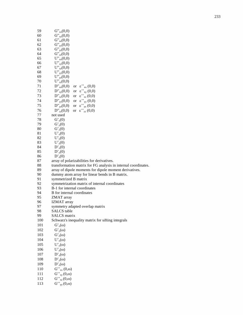
233

59 G”xx(0,0)

60 G”xy(0,0)

61 G”xz(0,0)

62 G”yy(0,0)

63 G”yz(0,0)

64 G”zz(0,0)

65 U”xx(0,0)

66 U”xy(0,0)

67 U”xz(0,0)

68 U”yy(0,0)

69 U”yz(0,0)

70 U”zz(0,0)

71 D”xx(0,0) or ’’xx (0,0)

72 D”xy(0,0) or ’’xy (0,0)

73 D”xz(0,0) or ’’xz (0,0)

74 D”yy(0,0) or ’’yy (0,0)

75 D”yz(0,0) or ’’yz (0,0)

76 D”zz(0,0) or ’’zz (0,0)

77 not used

78 G’x(0)

79 G’y(0)

80 G’z(0)

81 U’x(0)

82 U’y(0)

83 U’z(0)

84 D’x(0)

85 D’y(0)

86 D’z(0)

87 array of polarizabilities for derivatives.

88 transformation matrix for FG analysis in internal coordinates.

89 array of dipole moments for dipole moment derivatives.

90 dummy atom array for linear bends in B matrix.

91 symmetrized B matrix

92 symmetrization matrix of internal coordinates

93 B-1 for internal coordinates

94 B for internal coordinates

95 ZMAT array

96 IZMAT array

97 symmetry adapted overlap matrix

98 SALCS table

99 SALCS matrix

100 Schwarz's inequality matrix for sifting integrals

101 G’x()

102 G’y()

103 G’z()

104 U’x()

105 U’y()

106 U’z()

107 D’x()

108 D’y()

109 D’z()

110 G’’xx (0,)

111 G’’xy (0,)

112 G’’xz (0,)

113 G’’yy (0,)

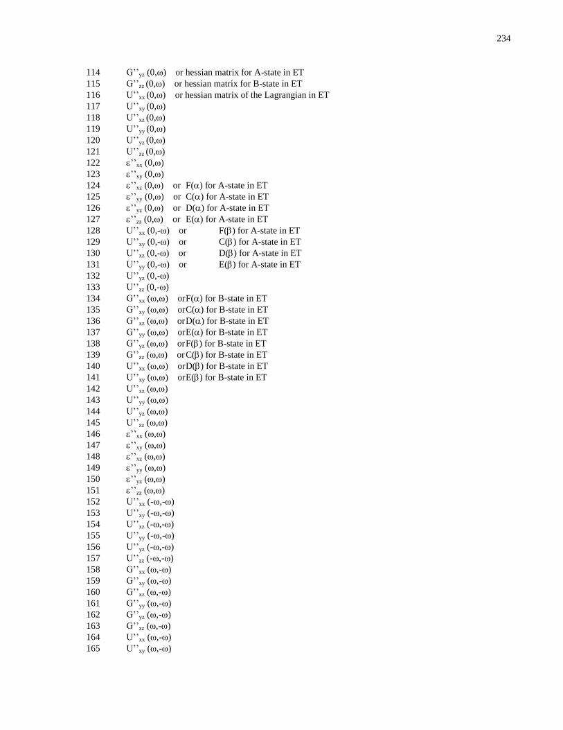
234

114 G’’yz (0,) or hessian matrix for A-state in ET

115 G’’zz (0,) or hessian matrix for B-state in ET

116 U’’xx (0,) or hessian matrix of the Lagrangian in ET

117 U’’xy (0,)

118 U’’xz (0,)

119 U’’yy (0,)

120 U’’yz (0,)

121 U’’zz (0,)

122 ’’xx (0,)

123 ’’xy (0,)

124 ’’xz (0,) or F() for A-state in ET

125 ’’yy (0,) or C() for A-state in ET

126 ’’yz (0,) or D() for A-state in ET

127 ’’zz (0,) or E() for A-state in ET

128 U’’xx (0,-) or F() for A-state in ET

129 U’’xy (0,-) or C() for A-state in ET

130 U’’xz (0,-) or D() for A-state in ET

131 U’’yy (0,-) or E() for A-state in ET

132 U’’yz (0,-)

133 U’’zz (0,-)

134 G’’xx (,) or F() for B-state in ET

135 G’’xy (,) or C() for B-state in ET

136 G’’xz (,) or D() for B-state in ET

137 G’’yy (,) or E() for B-state in ET

138 G’’yz (,) or F() for B-state in ET

139 G’’zz (,) or C() for B-state in ET

140 U’’xx (,) or D() for B-state in ET

141 U’’xy (,) or E() for B-state in ET

142 U’’xz (,)

143 U’’yy (,)

144 U’’yz (,)

145 U’’zz (,)

146 ’’xx (,)

147 ’’xy (,)

148 ’’xz (,)

149 ’’yy (,)

150 ’’yz (,)

151 ’’zz (,)

152 U’’xx (-,-)

153 U’’xy (-,-)

154 U’’xz (-,-)

155 U’’yy (-,-)

156 U’’yz (-,-)

157 U’’zz (-,-)

158 G’’xx (,-)

159 G’’xy (,-)

160 G’’xz (,-)

161 G’’yy (,-)

162 G’’yz (,-)

163 G’’zz (,-)

164 U’’xx (,-)

165 U’’xy (,-)

235

166 U’’xz (,-)

167 U’’yy (,-)

168 U’’yz (,-)

169 U’’zz (,-)

170 ’’xx (,-)

171 ’’xy (,-)

172 ’’xz (,-)

173 ’’yy (,-)

174 ’’yz (,-)

175 ’’zz (,-)

176 U’’xx (-,)

177 U’’xy (-,)

178 U’’xz (-,)

179 U’’yy (-,)

180 U’’yz (-,)

181 U’’zz (-,)

182 D’’xx (-,-) or D’’’xxx

183 D’’xy (-,-) or D’’’xxy

184 D’’xz (-,-) or D’’’xxz

185 D’’yy (-,-) or D’’’xyy

186 D’’yz (-,-) or D’’’xyz

187 D’’zz (-,-) or D’’’xzz

188 D’’’yyy

189 D’’’yyz

190 D’’’yzz

191 D’’’zzz or G’x (2 )

192 G’y (2 )

193 G’z (2 )

194 U’x (2 )

195 U’y (2 )

196 U’z (2 )

197 not used

198 G’x (3 )

199 G’y (3 )

200 G’z (3 )

201 U’x (3 )

202 U’y (3 )

203 U’z (3 )

Note that the master file DA10 index array is 255 word long but only 254 records may be used. One word is reserved for

the system.

236

How to read the tape on AIX/RS6000

The 1/4" tape was created with the following command:

Tar -cvhf /dev/rmt0 .

We assume that the directory /u/chemstat exits. To unload the tape, execute the following commands:

cd /u/chemstat

tar -xvf /dev/rmt0

Note that the name of the tape device on your AIX workstation may be different. All the files included on the tape get

copied into the current directory /u/chemstat/hondo in the subdirectory ./master for the serial ‘master’ code and the

subdirectories ./poe , ./mpi , ./pvm3 , ./tcg for the parallel versions.

237

How to run HONDOPLUS

Assuming that the directory in which the HONDOPLUS executable module is in your PATH variable (define PATH in your

.kshrc file or .cshrc file) the program can be run by issuing this command:

hondo.x input-file-name output-file-name

where 'input-file-name' and 'output-file-name' are the names of the input and output files. For example to execute the

sample1.hnd data included with the program, one should issue the following command:

cd hondoplus-v5.2/master/samples

hondo.x sample1.hnd sample1.out

If 'input-file-name' and 'output-file-name' are not supplied the program prompts for them. If you don't give a filename after

the prompt for the output file the screen (the standard output in the AIX terminology) will we used.

The program supports absolute or relative path names, as long as the total length of the file name is less than 80 characters.

By default, the punch file will be placed in the same directory as the output file and all the other files created by the

program while executing, will go in the directory from which the program is executed. A different path to any other

directory to be used for these scratch files can be specified via the SCRPATH variable. For example if you are running

under the ksh shell, you may include the following statement in your .profile file or your .kshrc file:

export SCRPATH=/tmp

and the /tmp directory will be used to hold the scratch files. Alternately a different SCRPATH can be specified by using the

$FIL namelist. The definitions given in namelist $FIL take precedence over the definition of the SCRPATH variable. The

namelist $FIL is described on the next page.

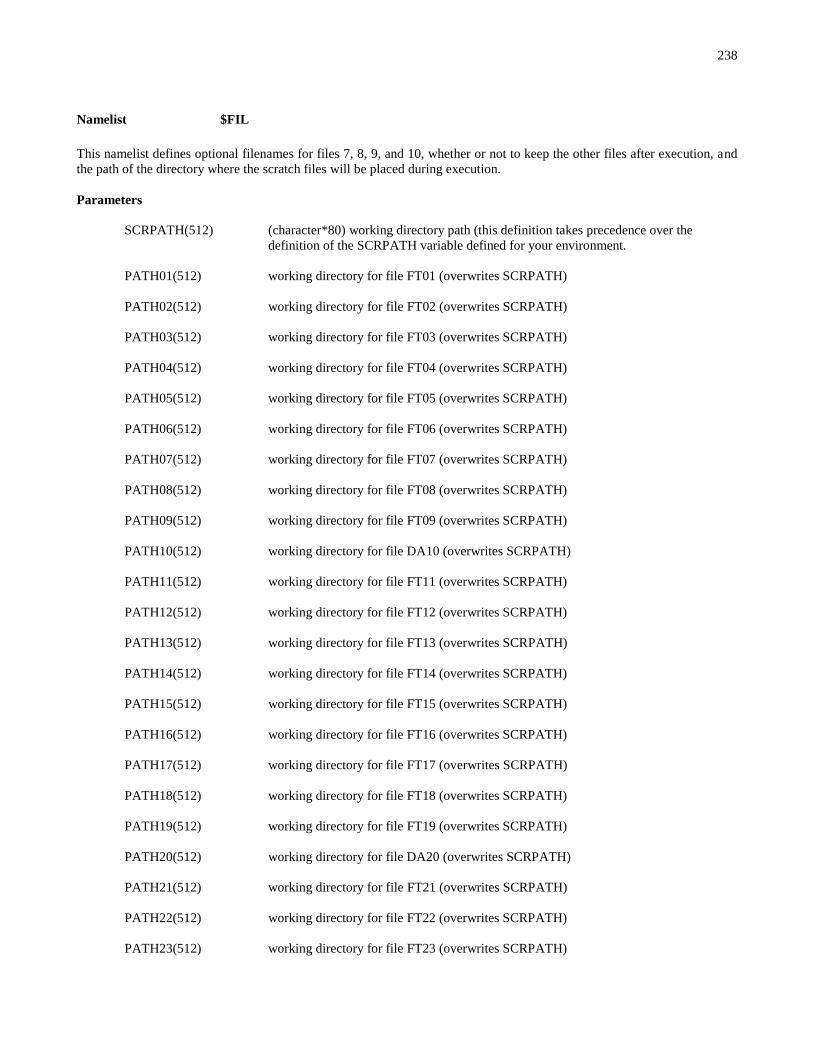
238

Namelist $FIL

This namelist defines optional filenames for files 7, 8, 9, and 10, whether or not to keep the other files after execution, and

the path of the directory where the scratch files will be placed during execution.

Parameters

SCRPATH(512) (character*80) working directory path (this definition takes precedence over the

definition of the SCRPATH variable defined for your environment.

PATH01(512) working directory for file FT01 (overwrites SCRPATH)









PATH10(512) working directory for file DA10 (overwrites SCRPATH)














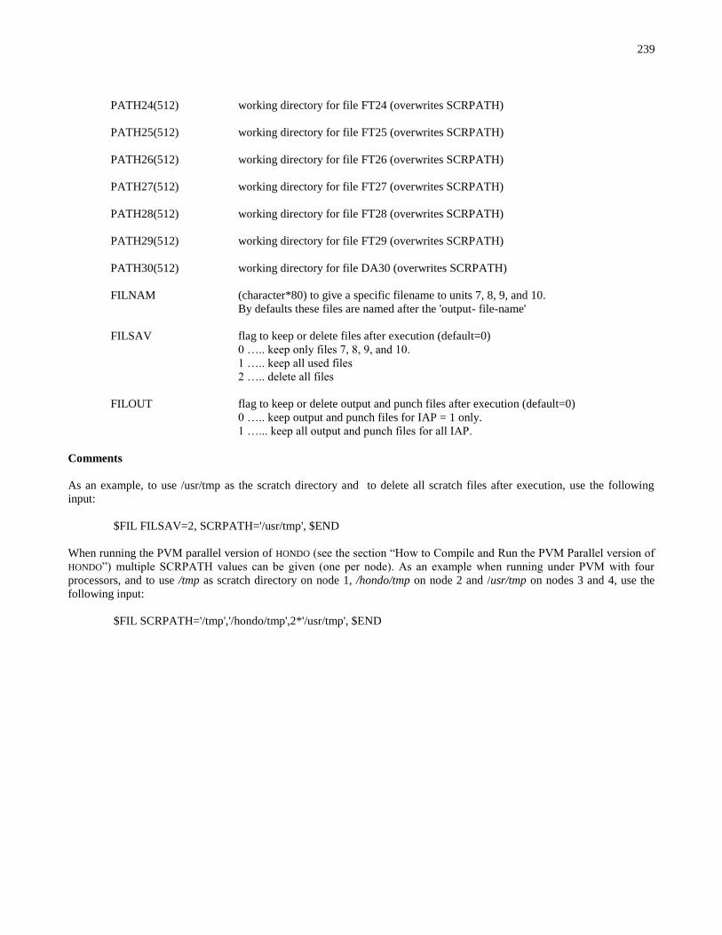
239








FILNAM (character*80) to give a specific filename to units 7, 8, 9, and 10.

By defaults these files are named after the 'output- file-name'

FILSAV flag to keep or delete files after execution (default=0)

0 ….. keep only files 7, 8, 9, and 10.

1 ….. keep all used files

2 ….. delete all files

FILOUT flag to keep or delete output and punch files after execution (default=0)

0 ….. keep output and punch files for IAP = 1 only.

1 …... keep all output and punch files for all IAP.

Comments

As an example, to use /usr/tmp as the scratch directory and to delete all scratch files after execution, use the following

input:

$FIL FILSAV=2, SCRPATH='/usr/tmp', $END

When running the PVM parallel version of HONDO (see the section “How to Compile and Run the PVM Parallel version of

HONDO”) multiple SCRPATH values can be given (one per node). As an example when running under PVM with four

processors, and to use /tmp as scratch directory on node 1, /hondo/tmp on node 2 and /usr/tmp on nodes 3 and 4, use the

following input:

$FIL SCRPATH='/tmp','/hondo/tmp',2*'/usr/tmp', $END

240

How to compile and Run the POE parallel version of HONDO

PVM is a software that makes it possible to run HONDO in a parallel mode, with the nodes being part of a local area network

(Ethernet or LAN) linked through TCP/IP. A parallel execution of HONDO with PVM requires additional input data which is

described in the next section for the namelist $PVM. In this section we only describe how to set up HONDO to run under

PVM.

Similarly to the /hondoplus-v5.2/master directory where all files for the serial program reside, a directory

/u/chemstat/hondo/pvm gets created when you read the tape. After compiling the serial version of the code, the PVM

parallel version can be created using the commands:

cd /hondoplus-v5.2/poe

make -f makefile.poe

The executable file will be called poe.hndand will be left in this directory. The makefile assumes that you have the POE

software installed and that it resides in the directory /hondoplus-v5.2/poe.

Remember that POE expects the different instances of a parallel program to be placed in the subdirectory hondoplus-

v5.2/poe of your login directory of every computer on which you want to run the program. So, you have to move or copy

the binary file poe.hnd to the appropriate directories. Only one binary module is created. It contains both the code for the

'host' and the 'nodes' (in the PVM terminology) and specific routines perform different tasks either for the 'host' or for the

'nodes'.

Once the pvmhnd file is installed in the appropriate directories and you start PVM (refer to your PVM users guide for this

matter) the program can be started with the same syntax as the serial program:

poe.hnd 'input-file-name' 'output-file-name'

The same rules apply to the input and output file names and the use of the SCRPATH variable is also similar. Only ONE

pvmhnd program can be running at a given one time for one user. If a POE job of HONDO stops due to errors, reset POE

before running again.

An alternate way of running the code is to use the shell script runpvm in which the number of nodes for the job is given. For

example :

runpoe sample1

The script appends the namelist $PVM to the input file sample1.hnd, so that it needs not be done explicitly by the user.

Note however that it is still critical to specify the scratch directory via the SCRPATH variable in the $FIL namelist to direct

the files to the right directory.

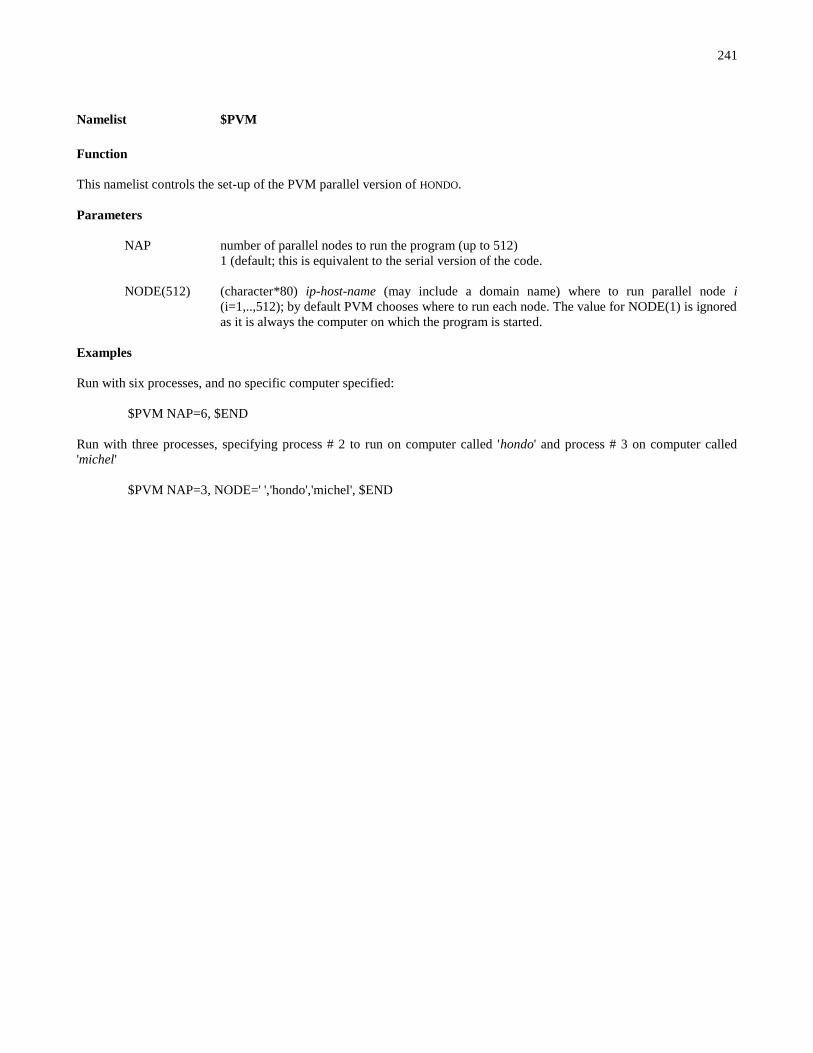
241

Namelist $PVM

Function

This namelist controls the set-up of the PVM parallel version of HONDO.

Parameters

NAP number of parallel nodes to run the program (up to 512)

1 (default; this is equivalent to the serial version of the code.

NODE(512) (character*80) ip-host-name (may include a domain name) where to run parallel node i

(i=1,..,512); by default PVM chooses where to run each node. The value for NODE(1) is ignored

as it is always the computer on which the program is started.

Examples

Run with six processes, and no specific computer specified:

$PVM NAP=6, $END

Run with three processes, specifying process # 2 to run on computer called 'hondo' and process # 3 on computer called

'michel'

$PVM NAP=3, NODE=' ','hondo','michel', $END

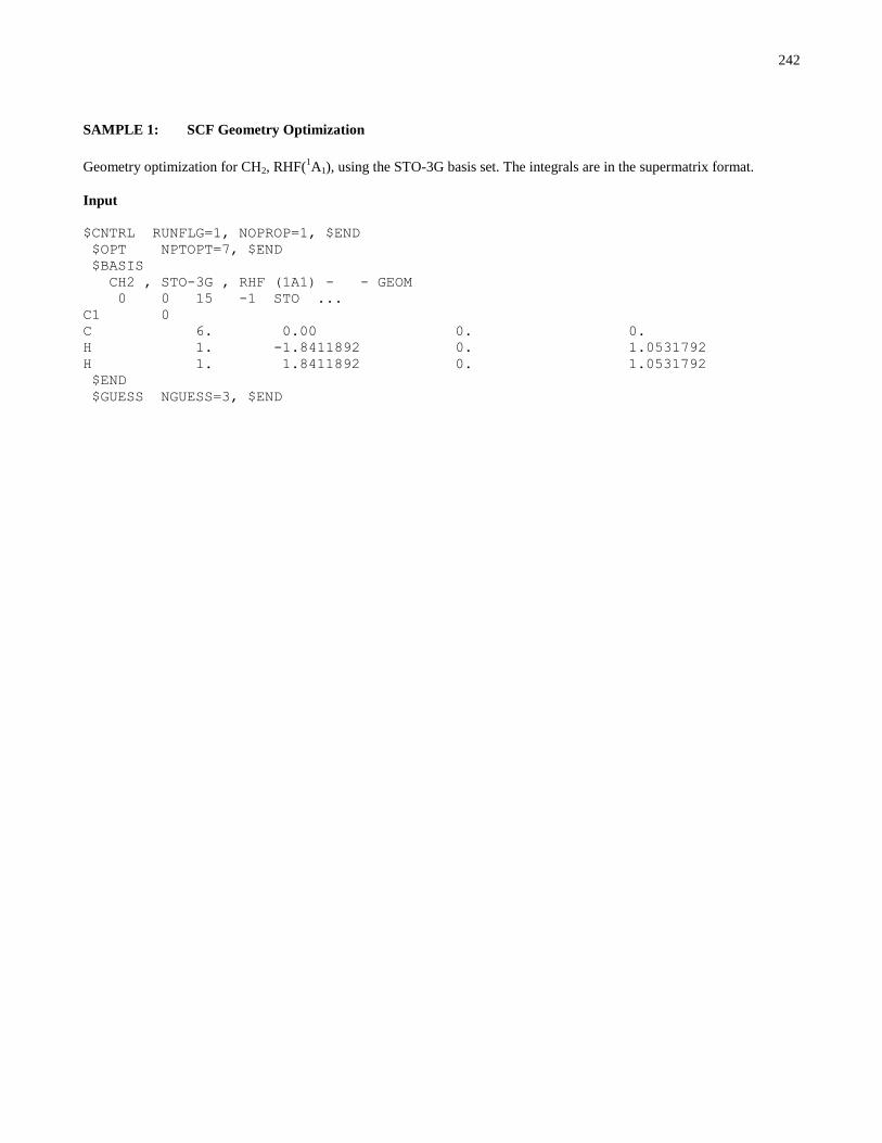
242

SAMPLE 1: SCF Geometry Optimization

Geometry optimization for CH2, RHF(1A1), using the STO-3G basis set. The integrals are in the supermatrix format.

Input

$CNTRL RUNFLG=1, NOPROP=1, $END

$OPT NPTOPT=7, $END

$BASIS

CH2 , STO-3G , RHF (1A1) - - GEOM

0 0 15 -1 STO ...

C1 0

C 6. 0.00 0. 0.

H 1. -1.8411892 0. 1.0531792

H 1. 1.8411892 0. 1.0531792

$END

$GUESS NGUESS=3, $END

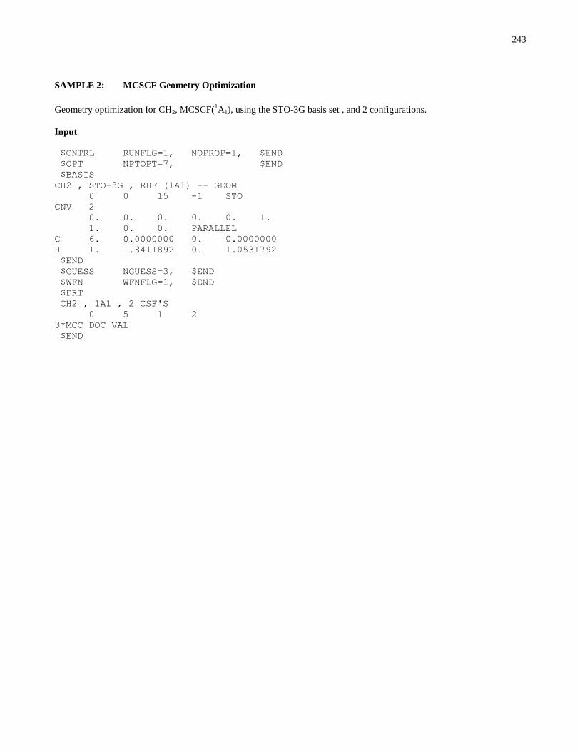
243

SAMPLE 2: MCSCF Geometry Optimization

Geometry optimization for CH2, MCSCF(1A1), using the STO-3G basis set , and 2 configurations.

Input


$OPT NPTOPT=7, $END

$BASIS

CH2 , STO-3G , RHF (1A1) -- GEOM

0 0 15 -1 STO

CNV 2

0. 0. 0. 0. 0. 1.

1. 0. 0. PARALLEL

C 6. 0.0000000 0. 0.0000000

H 1. 1.8411892 0. 1.0531792

$END


$WFN WFNFLG=1, $END

$DRT

CH2 , 1A1 , 2 CSF'S

0 5 1 2

3*MCC DOC VAL

$END

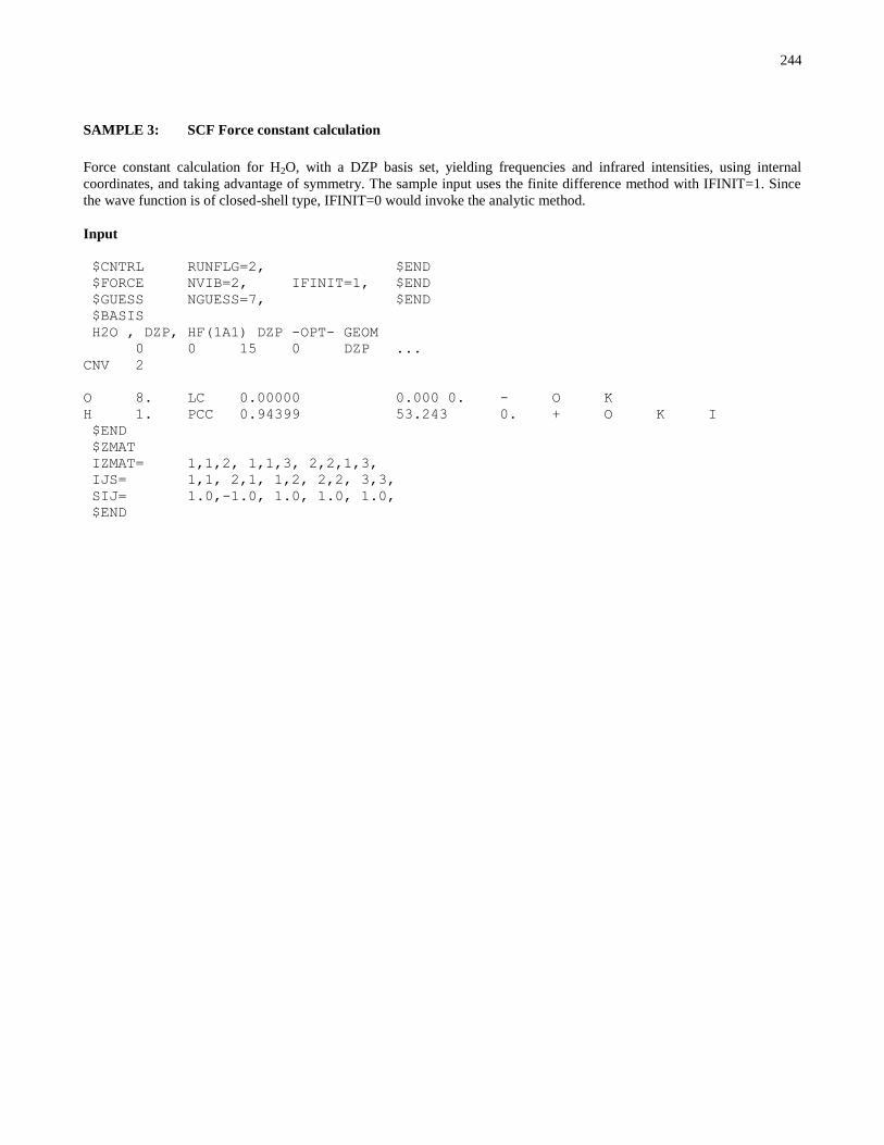
244

SAMPLE 3: SCF Force constant calculation

Force constant calculation for H2O, with a DZP basis set, yielding frequencies and infrared intensities, using internal

coordinates, and taking advantage of symmetry. The sample input uses the finite difference method with IFINIT=1. Since

the wave function is of closed-shell type, IFINIT=0 would invoke the analytic method.

Input


$FORCE NVIB=2, IFINIT=1, $END


$BASIS

H2O , DZP, HF(1A1) DZP -OPT- GEOM

0 0 15 0 DZP ...

CNV 2

O 8. LC 0.00000 0.000 0. - O K

H 1. PCC 0.94399 53.243 0. + O K I

$END

$ZMAT

IZMAT= 1,1,2, 1,1,3, 2,2,1,3,

IJS= 1,1, 2,1, 1,2, 2,2, 3,3,

SIJ= 1.0,-1.0, 1.0, 1.0, 1.0,

$END

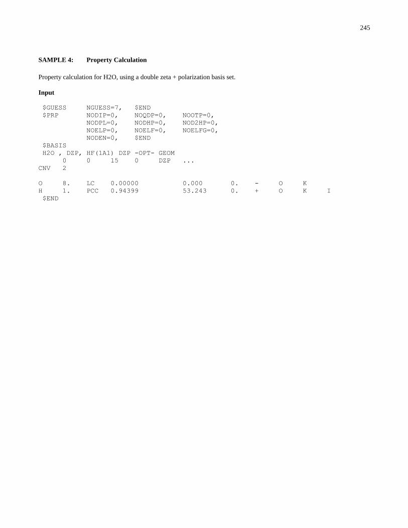
245

SAMPLE 4: Property Calculation

Property calculation for H2O, using a double zeta + polarization basis set.

Input


$PRP NODIP=0, NOQDP=0, NOOTP=0,

NODPL=0, NODHP=0, NOD2HP=0,

NOELP=0, NOELF=0, NOELFG=0,

NODEN=0, $END

$BASIS


0 0 15 0 DZP ...

CNV 2

O 8. LC 0.00000 0.000 0. - O K

H 1. PCC 0.94399 53.243 0. + O K I

$END

246

SAMPLE 5: CI calculation

Singles and doubles CI calculation for H2O (1A1) using a double zeta basis set.

Input

$GUESS NGUESS=5, NORB=13, $END

$WFN WFNFLG=2, $END

$DRT

H2O , DZ , SDCI(1A1)

4 13 1 2

FZC1 DOC1 DOC4 DOC1 DOC3

UOC1 UOC4 UOC3 UOC1 UOC4 UOC1 UOC4 UOC1

$END

$BASIS

H2O , DZP, HF(1A1) DZP -OPT- GEOM 00150DZV...

CNV 2

O 8. LC 0.00000 0.000 0. - O K

H 1. PCC 0.94399 53.243 0. + O K I

$END

----- H2O , DZ , SCF(1A1) ORBS. -----

$VEC

1 1 0.99969348E+00 -0.35673499E-04 0.18350280E-02 0.00000000E+00

0.00000000E+00

1 2 0.16795255E-02 0.00000000E+00 0.00000000E+00 -0.47950764E-03

0.15179226E-04

1 3 -0.15768075E-03 0.15179226E-04 -0.15768075E-03

2 1 -0.22685420E+00 0.48333446E+00 0.44233916E+00 0.00000000E+00

0.00000000E+00

2 2 0.13025525E+00 0.00000000E+00 0.00000000E+00 0.30415605E-01

0.14092914E+00

2 3 0.77850030E-02 0.14092914E+00 0.77850030E-02

3 1 0.00000000E+00 0.00000000E+00 0.00000000E+00 -0.57565476E+00

0.00000000E+00

3 2 0.00000000E+00 -0.17388627E+00 0.00000000E+00 0.00000000E+00

0.26096223E+00

3 3 0.12675513E+00 -0.26096223E+00 -0.12675513E+00

4 1 0.80029347E-01 -0.18659035E+00 -0.26389034E+00 0.00000000E+00

0.00000000E+00

4 2 0.63048913E+00 0.00000000E+00 0.00000000E+00 0.33271237E+00

0.13781987E+00

4 3 0.52484302E-01 0.13781987E+00 0.52484302E-01

5 1 0.00000000E+00 0.00000000E+00 0.00000000E+00 0.00000000E+00 -

0.72831476E+00

5 2 0.00000000E+00 0.00000000E+00 -0.40952745E+00 0.00000000E+00

0.00000000E+00

5 3 0.00000000E+00 0.00000000E+00 0.00000000E+00

6 1 0.95200975E-01 -0.10094780E+00 -0.12143837E+01 0.00000000E+00

0.00000000E+00

6 2 -0.25064454E+00 0.00000000E+00 0.00000000E+00 -0.45449995E+00

0.53553428E-01

6 3 0.10126232E+01 0.53553428E-01 0.10126232E+01

7 1 0.00000000E+00 0.00000000E+00 0.00000000E+00 -0.37654132E+00

0.00000000E+00

247

7 2 0.00000000E+00 -0.99657376E+00 0.00000000E+00 0.00000000E+00 -

0.32323489E-01

7 3 -0.16180265E+01 0.32323489E-01 0.16180265E+01

8 1 0.00000000E+00 0.00000000E+00 0.00000000E+00 0.00000000E+00

0.90205939E+00

8 2 0.00000000E+00 0.00000000E+00 -0.10846386E+01 0.00000000E+00

0.00000000E+00

8 3 0.00000000E+00 0.00000000E+00 0.00000000E+00

9 1 -0.39548763E-01 0.74832795E-01 0.39369175E+00 0.00000000E+00

0.00000000E+00

9 2 -0.86211064E+00 0.00000000E+00 0.00000000E+00 0.13029422E+01 -

0.16777278E+00

9 3 -0.26131858E+00 -0.16777278E+00 -0.26131858E+00

10 1 0.00000000E+00 0.00000000E+00 0.00000000E+00 -0.43937112E+00

0.00000000E+00

10 2 0.00000000E+00 0.16679456E+01 0.00000000E+00 0.00000000E+00

0.63236301E+00

10 3 0.41408054E+00 -0.63236301E+00 -0.41408054E+00

11 1 -0.82848457E-01 0.38057101E+00 -0.11151897E+00 0.00000000E+00

0.00000000E+00

11 2 0.41311856E+00 0.00000000E+00 0.00000000E+00 0.17010874E+00 -

0.98806011E+00

11 3 0.51051177E+00 -0.98806011E+00 0.51051177E+00

12 1 0.00000000E+00 0.00000000E+00 0.00000000E+00 0.92049575E+00

0.00000000E+00

12 2 0.00000000E+00 -0.10363303E+01 0.00000000E+00 0.00000000E+00

0.72446919E+00

12 3 -0.12504387E+01 -0.72446919E+00 0.12504387E+01

13 1 -0.10033470E+00 0.18731916E+01 -0.29447169E+01 0.00000000E+00

0.00000000E+00

13 2 0.26582590E-01 0.00000000E+00 0.00000000E+00 -0.68725435E+00

0.38613350E+00

13 3 0.66298501E+00 0.38613350E+00 0.66298501E+00

$END

248

SAMPLE 6: MP2 calculation

MP2 calculation for H2O, using a double zeta + polarization basis set, and taking advantage of symmetry.

Input

$CNTRL NOPROP=1, $END

$WFN WFNFLG=5, $END

$BASIS


0 0 15 0 DZP ...

CNV 2

O 8. LC 0.00000 0.000 0. - O K

H 1. PCC 0.94399 53.243 0. + O K I

$END

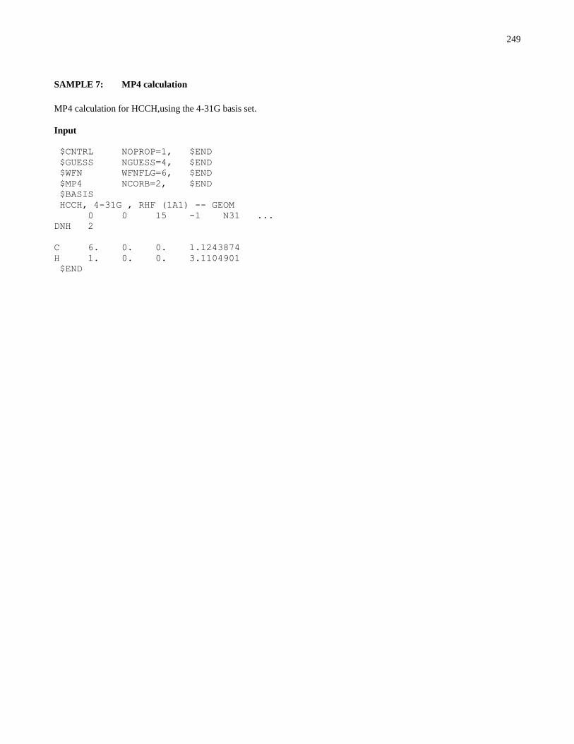
249

SAMPLE 7: MP4 calculation

MP4 calculation for HCCH,using the 4-31G basis set.

Input

$CNTRL NOPROP=1, $END


$WFN WFNFLG=6, $END

$MP4 NCORB=2, $END

$BASIS

HCCH, 4-31G , RHF (1A1) -- GEOM

0 0 15 -1 N31 ...

DNH 2

C 6. 0. 0. 1.1243874

H 1. 0. 0. 3.1104901

$END

250

SAMPLE 8: ECP Calculation

This example shows how to run an ECP calculation.

Input


$SCF MOPRT=10, $END

$BASIS

FORMIC ACID, HF(1A1) -CEP31G- , -OPT- GEOM

0 0 15 0 ... ECP

C1

C 6. LC 2.00000 0 .0. + O I

1 SP 3

1 4.286 -0.14722 0.10257

2 1.046 0.08125 0.32987

3 0.3447 0.71360 0.48212

2SP1

1 0.1128 1.00000 1.00000

H 1. LC 1.09480 0. 0. + 1 O

1 S 3

1 13.013372 0.019678

2 1.962496 0.137952

3 0.444569 0.478313

2 S 1

1 0.121953 1.000000

O 8. PTC 1.21808 125.05 0. + 1 2 J

1 SP3

1 8.519 -0.14551 0.11007

2 2.073 0.08286 0.34969

3 0.6471 0.74325 0.48093

2 SP 1

1 0.2000 1.00000 1.00000

O 8. PTC 1.35944 110.72 0. - 1 2 J

1 SP 3

1 8.519 -0.14551 0.11007

2 2.073 0.08286 0.34969

3 0.647 1 0.7432 5 0.48093

2 SP 1

1 0.2000 1.00000 1.00000

H 1. PTC 0.96964 113.75 0. - 4 1 2

1 S 3

1 13.013372 0.019678

2 1.962496 0.137952

3 0.444569 0.478313

2 S 1

1 0.121953 1.000000

$END

$ECP FOR FORMIC ACID MONOMER

C-ECP 2 1

251

1

-0.89371 1 8.56468

2

1.92926 0 2.81497

14.88199 2 8.11296

O-ECP 2 1

1 -----OXYGEN U(P)-----

-0.92550 1 16.11718

-----OXYGEN U(S-P)-----

1.96069 0 5.05348

29.13442 2 15.95333

O-ECP 2 1

$END

252

SAMPLE 9: MIXED BASIS SET calculation

This example shows how to use a basis set made of bases stored in the program augmented with functions not internally

stored, for example the 6-31G** basis set.

Input


$BASIS

CH2 , 6-31G** , RHF (1A1)

0 0 15 -1 ... ...

C1 0

C 6. 0.0000000 0. 0.0000000

1 SV 6 N 31

2 D 1

1 0.80000 1.

H 1. -1.8411892 0. 1.0531792

1 SV 6 N31

2 P 1

1 1.00000 1.

H 1. 1.8411892 0. 1.0531792

1 SV 6 N31

2 P 1

1 1.00000 1.

$END

253

SAMPLE 10: GENERAL BASIS SET calculation

This example shows how to input a basis set that is not stored in the program, in the present case a MINI-3 basis set.

Input


$BASIS

CO , RHF(1A1) , HUZINAGA'S MINI-3 (43/4/1/1)

0 0 15 1 ... ...

C1

C 6. 0.00000000 0.00000000 0.0000000

1 S 4

1 451.90190 0.0194301

2 67.995770 0.1340007

3 15.144230 0.4591025

4 3.9684300 0.5293728

2 S 3

1 5.4007700 -.0834901

2 0.4639500 0.5783904

3 0.1473600 0.5023303

3 P 4

1 9.4746000 0.0379002

2 2.0071400 0.2089513

3 0.5462100 0.5088232

4 0.1517100 0.4692930

4 D 1

1 0.2880000 1.0000000

5 D 1

1 1.3350000 1.0000000

O 8. 1.08000000 0.00000000 0.0000000

1 S 4

1 821.83934 0.0191699

2 123.68182 0.1328095

3 27.666170 0.4594583

4 7.2995700 0.5290081

2 S 3

1 10.606960 -.0829300

2 0.9176400 0.5765903

3 0.2831700 0.5067003

3 P 4

1 17.750370 0.0428103

2 3.8646800 0.2283317

3 1.0477200 0.5088438

4 0.2756000 0.4611135

4 D 1

1 0.535 1.0000000

5 D 1

1 2.704 1.0000000

$END

254

SAMPLE 11: MP2 Geometry Optimization

Geometry optimization for CH3CH2OH, using the STO-3G basis set.

Input



$WFN WFNFLG=5, $END

$ZMAT IZMAT= 1,2,1,

1,3,1, 2,3,1,2,

1,4,2, 2,4,2,1, 3,4,2,1,3,

1,5,2, 2,5,2,1, 3,5,2,1,3,

1,6,2, 2,6,2,1, 3,6,2,1,3,

1,7,4, 2,7,4,2, 3,7,4,2,1,

1,8,4, 2,8,4,2, 3,8,4,2,1,

1,9,4, 2,9,4,2, 3,9,4,2,1,

$END

$BASIS

EtOHMP2 geometry optimization

0 0 15 -1 STO

CS

O 8. 2.3020449353 -0.4552053475 0.0000000000

C 6. 0.0288528235 1.0251664094 0.0000000000

H 1. 3.6717200209 0.8217894353 0.0000000000

C 6. -2.2509221556 -0.7884498859 0.0000000000

H 1. -0.0647831217 2.2516610293 1.6695537451

H 1. -2.2061826459 -1.9859565326 1.6650125467

H 1. -4.0041906824 0.2774035222 0.0000000000

$END

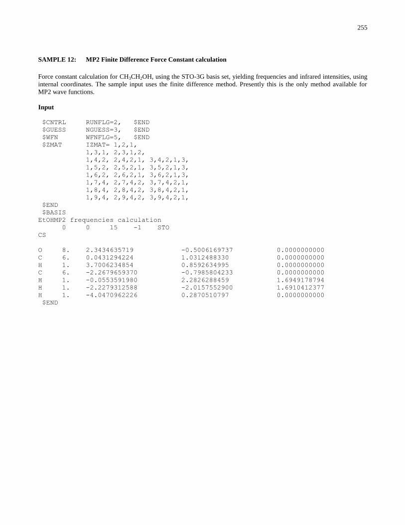
255

SAMPLE 12: MP2 Finite Difference Force Constant calculation

Force constant calculation for CH3CH2OH, using the STO-3G basis set, yielding frequencies and infrared intensities, using

internal coordinates. The sample input uses the finite difference method. Presently this is the only method available for

MP2 wave functions.

Input



$WFN WFNFLG=5, $END

$ZMAT IZMAT= 1,2,1,

1,3,1, 2,3,1,2,

1,4,2, 2,4,2,1, 3,4,2,1,3,

1,5,2, 2,5,2,1, 3,5,2,1,3,

1,6,2, 2,6,2,1, 3,6,2,1,3,

1,7,4, 2,7,4,2, 3,7,4,2,1,

1,8,4, 2,8,4,2, 3,8,4,2,1,

1,9,4, 2,9,4,2, 3,9,4,2,1,

$END

$BASIS

EtOHMP2 frequencies calculation

0 0 15 -1 STO

CS

O 8. 2.3434635719 -0.5006169737 0.0000000000

C 6. 0.0431294224 1.0312488330 0.0000000000

H 1. 3.7006234854 0.8592634995 0.0000000000

C 6. -2.2679659370 -0.7985804233 0.0000000000

H 1. -0.0553591980 2.2826288459 1.6949178794

H 1. -2.2279312588 -2.0157552900 1.6910412377

H 1. -4.0470962226 0.2870510797 0.0000000000

$END

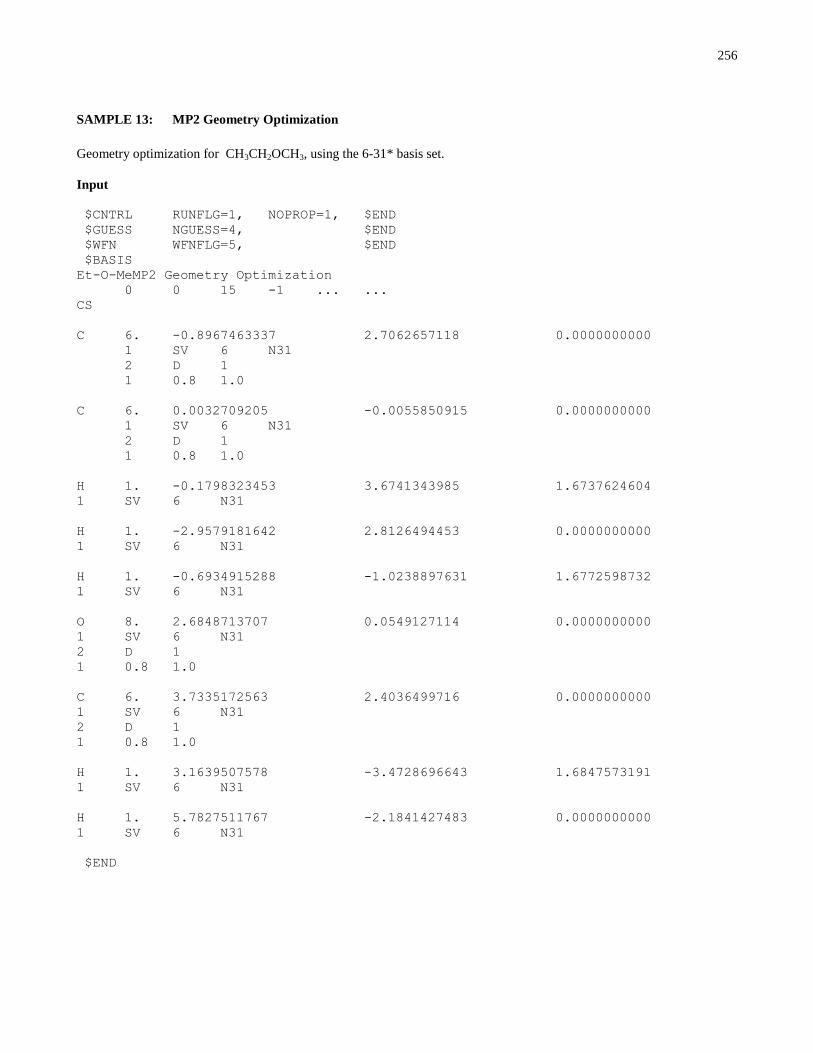
256

SAMPLE 13: MP2 Geometry Optimization

Geometry optimization for CH3CH2OCH3, using the 6-31* basis set.

Input



$WFN WFNFLG=5, $END

$BASIS

Et-O-MeMP2 Geometry Optimization

0 0 15 -1 ... ...

CS

C 6. -0.8967463337 2.7062657118 0.0000000000

1 SV 6 N31

2 D 1

1 0.8 1.0

C 6. 0.0032709205 -0.0055850915 0.0000000000

1 SV 6 N31

2 D 1

1 0.8 1.0

H 1. -0.1798323453 3.6741343985 1.6737624604

1 SV 6 N31

H 1. -2.9579181642 2.8126494453 0.0000000000

1 SV 6 N31

H 1. -0.6934915288 -1.0238897631 1.6772598732

1 SV 6 N31

O 8. 2.6848713707 0.0549127114 0.0000000000

1 SV 6 N31

2 D 1

1 0.8 1.0

C 6. 3.7335172563 2.4036499716 0.0000000000

1 SV 6 N31

2 D 1

1 0.8 1.0

H 1. 3.1639507578 -3.4728696643 1.6847573191

1 SV 6 N31

H 1. 5.7827511767 -2.1841427483 0.0000000000

1 SV 6 N31

$END

257

SAMPLE 14: RHF Analytical Force Constant Calculation

Force constant calculation for trans-(NH2)CH=CH(NO2) using the STO-3G basis set and internal coordinates.

Input


$FORCE IFINIT=0, $END

$ZMAT IZMAT=1,2,1,

1,3,1, 2,3,1,2,

1,4,2, 2,4,2,1, 3,4,2,1,3,

1,5,1, 2,5,1,2, 3,5,1,2,8,

1,6,5, 2,6,5,1, 3,6,5,1,2,

1,7,5, 2,7,5,1, 3,7,5,1,2,

1,8,2, 2,8,2,1, 3,8,2,1,3,

1,9,8, 2,9,8,2, 3,9,8,2,1,

1,10,8, 2,10,8,2, 3,10,8,2,1,

$END

$BASIS

trans-(H2N)CH=CH(NO2) hessian calculation

0 0 15 -1 STO

CS

C 6. 2.7879229075 0.1184877622 0.0000000000

C 6. 4.1370510203 -1.9940856985 0.0000000000

H 1. 3.4965556995 2.0289322254 0.0000000000

H 1. 3.1392802453 -3.7967485187 0.0000000000

N 7. -0.0130100629 -0.0566108447 0.0000000000

O 8. -1.0503784912 -2.2482301722 0.0000000000

O 8. -1.2517621698 2.0198200831 0.0000000000

N 7. 6.7466377362 -2.1526912988 0.0000000000

H 1. 7.8339173693 -0.5741256742 0.0000000000

H 1. 7.6224857456 -3.8556478611 0.0000000000

$END

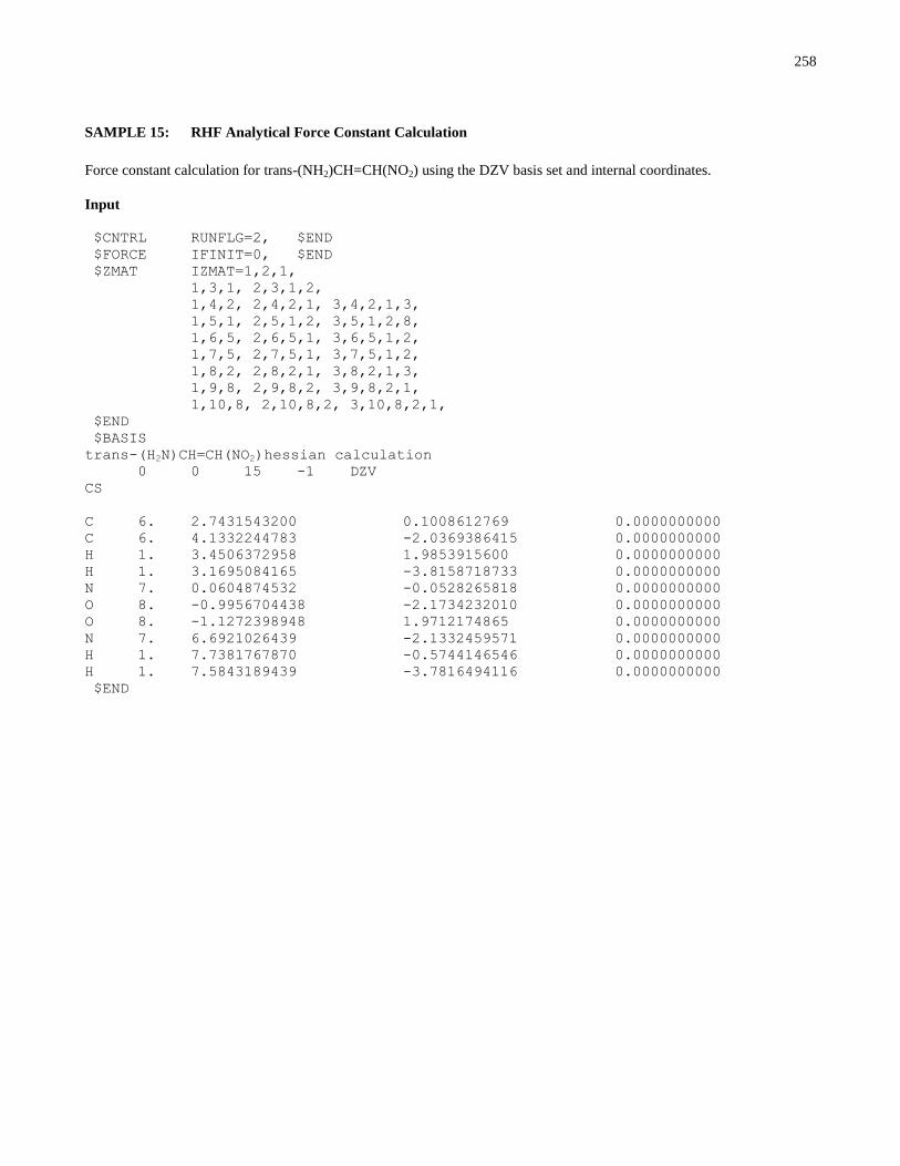
258

SAMPLE 15: RHF Analytical Force Constant Calculation

Force constant calculation for trans-(NH2)CH=CH(NO2) using the DZV basis set and internal coordinates.

Input


$FORCE IFINIT=0, $END

$ZMAT IZMAT=1,2,1,

1,3,1, 2,3,1,2,

1,4,2, 2,4,2,1, 3,4,2,1,3,

1,5,1, 2,5,1,2, 3,5,1,2,8,

1,6,5, 2,6,5,1, 3,6,5,1,2,

1,7,5, 2,7,5,1, 3,7,5,1,2,

1,8,2, 2,8,2,1, 3,8,2,1,3,

1,9,8, 2,9,8,2, 3,9,8,2,1,

1,10,8, 2,10,8,2, 3,10,8,2,1,

$END

$BASIS

trans-(H2N)CH=CH(NO2)hessian calculation

0 0 15 -1 DZV

CS

C 6. 2.7431543200 0.1008612769 0.0000000000

C 6. 4.1332244783 -2.0369386415 0.0000000000

H 1. 3.4506372958 1.9853915600 0.0000000000

H 1. 3.1695084165 -3.8158718733 0.0000000000

N 7. 0.0604874532 -0.0528265818 0.0000000000

O 8. -0.9956704438 -2.1734232010 0.0000000000

O 8. -1.1272398948 1.9712174865 0.0000000000

N 7. 6.6921026439 -2.1332459571 0.0000000000

H 1. 7.7381767870 -0.5744146546 0.0000000000

H 1. 7.5843189439 -3.7816494116 0.0000000000

$END

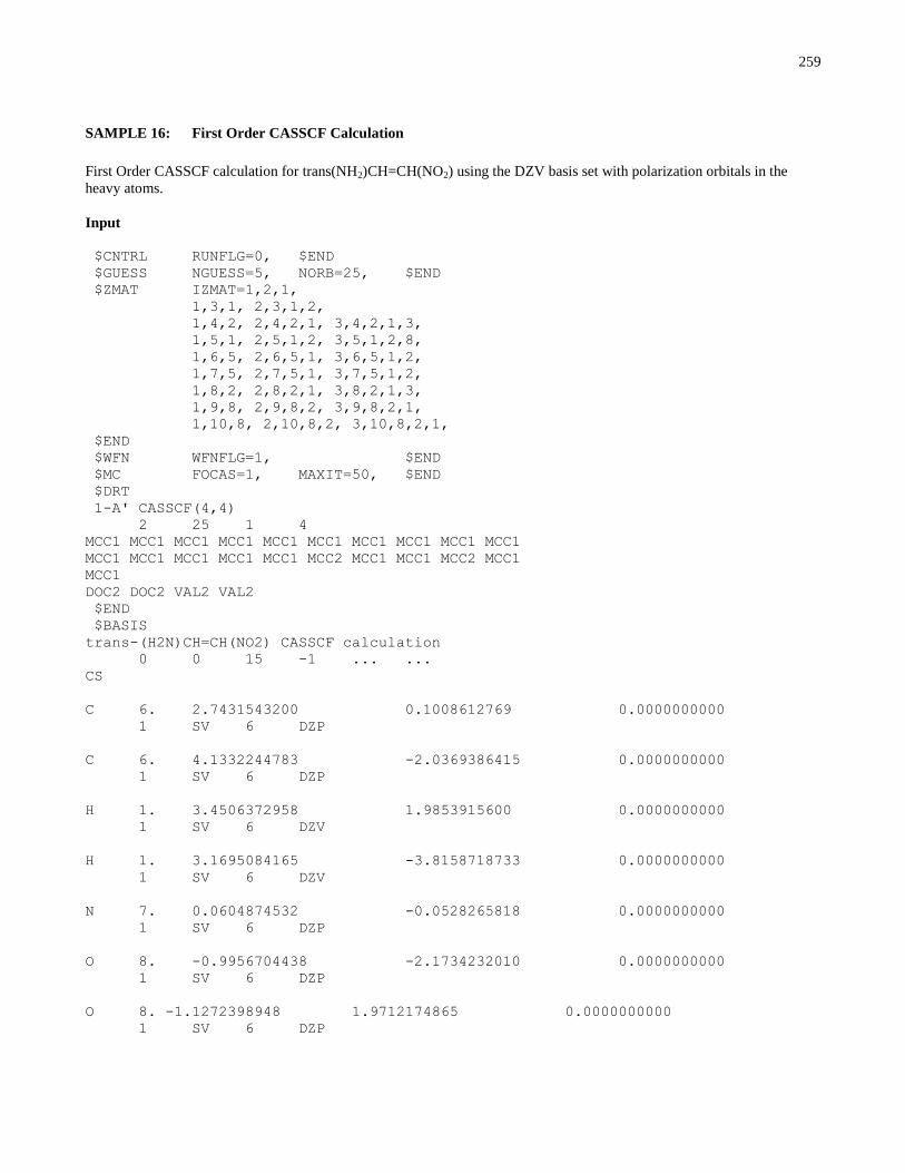
259

SAMPLE 16: First Order CASSCF Calculation

First Order CASSCF calculation for trans(NH2)CH=CH(NO2) using the DZV basis set with polarization orbitals in the

heavy atoms.

Input



$ZMAT IZMAT=1,2,1,

1,3,1, 2,3,1,2,

1,4,2, 2,4,2,1, 3,4,2,1,3,

1,5,1, 2,5,1,2, 3,5,1,2,8,

1,6,5, 2,6,5,1, 3,6,5,1,2,

1,7,5, 2,7,5,1, 3,7,5,1,2,

1,8,2, 2,8,2,1, 3,8,2,1,3,

1,9,8, 2,9,8,2, 3,9,8,2,1,

1,10,8, 2,10,8,2, 3,10,8,2,1,

$END

$WFN WFNFLG=1, $END

$MC FOCAS=1, MAXIT=50, $END

$DRT

1-A' CASSCF(4,4)

2 25 1 4

MCC1 MCC1 MCC1 MCC1 MCC1 MCC1 MCC1 MCC1 MCC1 MCC1

MCC1 MCC1 MCC1 MCC1 MCC1 MCC2 MCC1 MCC1 MCC2 MCC1

MCC1

DOC2 DOC2 VAL2 VAL2

$END

$BASIS

trans-(H2N)CH=CH(NO2) CASSCF calculation

0 0 15 -1 ... ...

CS

C 6. 2.7431543200 0.1008612769 0.0000000000

1 SV 6 DZP

C 6. 4.1332244783 -2.0369386415 0.0000000000

1 SV 6 DZP

H 1. 3.4506372958 1.9853915600 0.0000000000

1 SV 6 DZV

H 1. 3.1695084165 -3.8158718733 0.0000000000

1 SV 6 DZV

N 7. 0.0604874532 -0.0528265818 0.0000000000

1 SV 6 DZP

O 8. -0.9956704438 -2.1734232010 0.0000000000

1 SV 6 DZP

O 8. -1.1272398948 1.9712174865 0.0000000000

1 SV 6 DZP

260

N 7. 6.6921026439 -2.1332459571 0.0000000000

1 SV 6 DZP

H 1. 7.7381767870 -0.5744146546 0.0000000000

1 SV 6 DZV

H 1.7.5843189439 -3.7816494116 0.0000000000

1 SV 6 DZV

$END

$VEC

1 1-0.10794513E-05 0.85228210E-04-0.17961571E-03 0.35830648E-04 0.13573449E-05

1 2 0.00000000E+00 0.35263677E-03-0.40167206E-03 0.00000000E+00-0.94399513E-04

1 3-0.37519576E-04 0.19457865E-04 0.27063027E-05 0.00000000E+00 0.00000000E+00

1 4-0.53010571E-06-0.23211730E-04-0.21107204E-03-0.77207694E-05 0.68760223E-05

1 5 0.00000000E+00-0.39922192E-03-0.11420382E-03 0.00000000E+00 0.31492445E-04

1 6 0.12828801E-04-0.16817355E-04-0.12705841E-04 0.00000000E+00 0.00000000E+00

1 7 0.12050278E-04 0.20490101E-03 0.27646367E-05-0.20673971E-03 0.42663686E-05

.

…

.rest of the input vectors not shown here

…

25 8 0.18816169E-16-0.47441156E-14 0.80990209E-15-0.87600780E-16-0.23546914E+00

25 9-0.38797105E-14-0.22475813E-16-0.23140099E+00-0.96371191E-16 0.14202645E-15

25 10 0.16057248E-15-0.22782612E-16 0.28560213E-01 0.35720587E-02 0.10549828E-15

25 11-0.27339075E-16-0.17931192E-14 0.56557989E-16 0.68925100E-16 0.12650660E+00

25 12 0.15408709E-15-0.43672267E-15 0.12605847E+00 0.10436212E-15-0.55018000E-16

25 13 0.11791212E-15-0.87912452E-17-0.41201738E-02-0.72066941E-02 0.92379589E-16

25 14-0.92367672E-16-0.14621712E-14-0.30453440E-16-0.18487323E-15 0.10401987E+00

25 15 0.34308216E-15 0.22565928E-15 0.79950731E-01 0.85482975E-16-0.96468800E-16

25 16 0.90097698E-16 0.37544367E-16-0.47047513E-02 0.80797624E-02 0.19598178E-16

25 17 0.15286029E-15-0.29544536E-14 0.71413414E-16-0.35741912E-15 0.17484816E+00

25 18 0.93930961E-15-0.17473350E-14 0.36609158E+00-0.24393651E-18 0.18517162E-16

25 19 0.81788263E-16-0.90320703E-17 0.36210004E-01-0.17875490E-02-0.72380913E-16

25 20 0.69479254E-15-0.10743644E-15-0.31562328E-14

$END

261

SAMPLE 17: Frequency-dependent (hyper)polarizability calculation

Calculation of frequency-dependent hyper-polarizabilities for hydrogen fluoride HF using a DZ basis set.

Input

$SCF MOPRT=7, $END

$PRP NOFPL=0, NOFHP=0, NOF2HP=0, $END

$FPL WAVEL=6943.00, $END

$BASIS

HFTEST CALCULATION FOR DYNAMIC (HYPER)POLARIZABILY

0 0 15 1 ... ...

C1 1

H 1. 0.0 0.0 -0.45855

1 S 3

1 19.2406 0.032828

2 2.8992 0.231208

3 0.6534 0.817238

2 S 1

1 0.1776 1.0

F 9. 0.0 0.0 0.45855

1 S 6

1 9994.79 0.002017

2 1506.03 0.015295

3 350.269 0.073110

4 104.0530 0.246420

5 34.8432 0.612593

6 4.3688 0.242489

2 S 1

1 12.2164 1.0

3 S 1

1 1.2078 1.0

4 S 1

1 0.3634 1.0

5 P 4

1 44.3555 0.020868

2 10.0820 0.130092

3 2.9959 0.396219

4 0.9383 0.620368

6 P 1

1 0.2733 1.0

$END

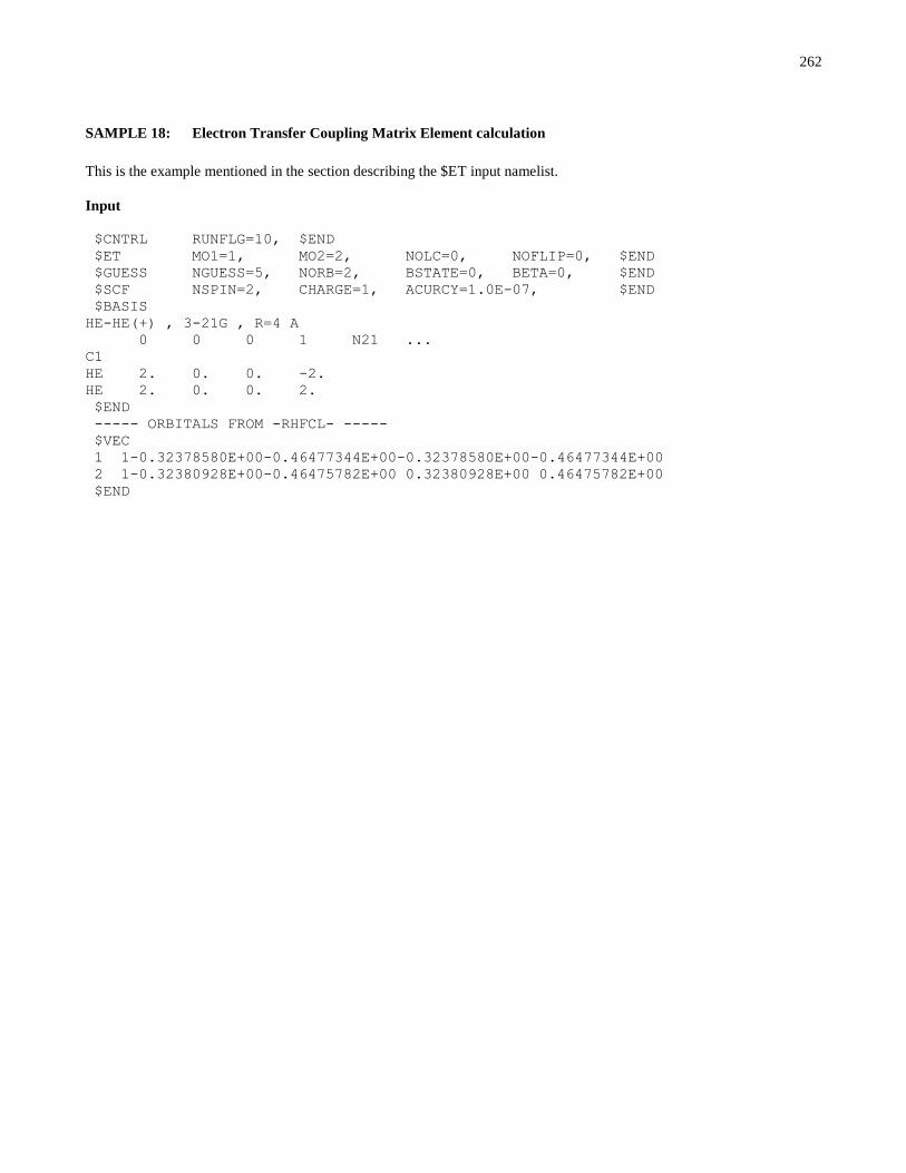
262

SAMPLE 18: Electron Transfer Coupling Matrix Element calculation

This is the example mentioned in the section describing the $ET input namelist.

Input


$ET MO1=1, MO2=2, NOLC=0, NOFLIP=0, $END

$GUESS NGUESS=5, NORB=2, BSTATE=0, BETA=0, $END


$BASIS

HE-HE(+) , 3-21G , R=4 A

0 0 0 1 N21 ...

C1

HE 2. 0. 0. -2.

HE 2. 0. 0. 2.

$END


$VEC

1 1-0.32378580E+00-0.46477344E+00-0.32378580E+00-0.46477344E+00

2 1-0.32380928E+00-0.46475782E+00 0.32380928E+00 0.46475782E+00

$END

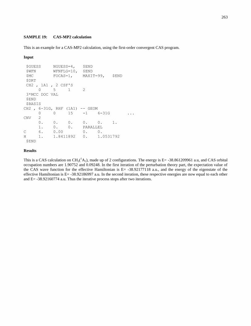
263

SAMPLE 19: CAS-MP2 calculation

This is an example for a CAS-MP2 calculation, using the first-order convergent CAS program.

Input


$WFN WFNFLG=10, $END

$MC FOCAS=1, MAXIT=99, $END

$DRT

CH2 , 1A1 , 2 CSF'S

0 5 1 2

3*MCC DOC VAL

$END

$BASIS

CH2 , 6-31G, RHF (1A1) -- GEOM

0 0 15 -1 6-31G ...

CNV 2

0. 0. 0. 0. 0. 1.

1. 0. 0. PARALLEL

C 6. 0.00 0. 0.

H 1. 1.8411892 0. 1.0531792

$END

Results

This is a CAS calculation on CH2(1A1), made up of 2 configurations. The energy is E= -38.861209961 a.u, and CAS orbital

occupation numbers are 1.90752 and 0.09248. In the first iteration of the perturbation theory part, the expectation value of

the CAS wave function for the effective Hamiltonian is E= -38.92177118 a.u., and the energy of the eigenstate of the

effective Hamiltonian is E= -38.92186997 a.u. In the second iteration, these respective energies are now equal to each other

and E= -38.92160774 a.u. Thus the iterative process stops after two iterations.

264

SAMPLE 20: MC-QDPT2 calculation

Example of MC-QDPT2 calculation.

Input

$CNTRL RUNFLG=0, NOPROP=1, IPRINT=0, NOSYM=0, ISPHER=1, $END



$CASMP2 IOPT=1, $END

$MCQDPT $END

$MCQDPT NEL=14, MULT=1,

NMOFZC=2, NMODOC=2, NMOACT=6, NMOEXT=18,

NSTATE=1, NSTCI=1, KSTATE=1, IFORB=1, ISTSYM=1, $END

$DRT

CO CASSCF (6 X 6)

0 10 1 6

2*FZC 2*MCC 3*DOC 3*VAL

$END

$BASIS

CO

0 0 15 0 .... ...

CNV 2

C 6. LC 0.0 0.0 0.0 - O I

1 S 8

1 6665.0000000 0.0006920000

2 1000.0000000 0.0053290000

3 228.0000000 0.0270770000

4 64.7100000 0.1017180000

5 21.0600000 0.2747400000

6 7.4950000 0.4485640000

7 2.7970000 0.2850740000

8 0.5215000 0.0152040000

2 S 8

1 6665.0000000 -0.0001460000

2 1000.0000000 -0.0011540000

3 228.0000000 -0.0057250000

4 64.7100000 -0.0233120000

5 21.0600000 -0.0639550000

6 7.4950000 -0.1499810000

7 2.7970000 -0.1272620000

8 0.5215000 0.5445290000

3 S 1

1 0.1596000 1.0000000000

4 P 3

1 9.4390000 0.0381090000

2 2.0020000 0.2094800000

3 0.5456000 0.5085570000

5 P 1

1 0.1517000 1.0000000000

6 D 1

1 0.5500000 1.0000000000

265

O1 8. LC 1.147392 0.0 0.0 + 1 K

1 S 8

1 11720.0000000 0.0007100000

2 1759.0000000 0.0054700000

3 400.8000000 0.0278370000

4 113.7000000 0.1048000000

5 37.0300000 0.2830620000

6 13.2700000 0.4487190000

7 5.0250000 0.2709520000

8 1.0130000 0.0154580000

2 S 8

1 11720.0000000 -0.0001600000

2 1759.0000000 -0.0012630000

3 400.8000000 -0.0062670000

4 113.7000000 -0.0257160000

5 37.0300000 -0.0709240000

6 13.2700000 -0.1654110000

7 5.0250000 -0.1169550000

8 1.0130000 0.5573680000

3 S 1

1 0.3023000 1.0000000000

4 P 3

1 17.7000000 0.0430180000

2 3.8540000 0.2289130000

3 1.0460000 0.5087280000

5 P 1

1 0.2753000 1.0000000000

6 D 1

1 1.1850000 1.0000000000

$END

----- MCHF ( CAN.CORE + CAN.VAL. + CAN.VIRT. ) ORBITALS -----

$VEC

1 1 .95795212D-04 -.77194487D-03 -.54998779D-03 .00000000D+00 .00000000D+00

1 2 -.21674159D-02 .00000000D+00 .00000000D+00 -.19293169D-02 .15569990D-03

1 3 .15569990D-03 -.31139981D-03 .00000000D+00 .00000000D+00 .00000000D+00

1 4 .10011907D+01 .22800939D-02 -.48502875D-02 .00000000D+00 .00000000D+00

1 5 .34748817D-02 .00000000D+00 .00000000D+00 -.38177567D-03 -.23019073D-03

1 6 -.23019073D-03 .46038147D-03 .00000000D+00 .00000000D+00 .00000000D+00

2 1 -.10014493D+01 .19235481D-02 .81577688D-02 .00000000D+00 .00000000D+00

2 2 .85427300D-02 .00000000D+00 .00000000D+00 .28927832D-02 .10872472D-02

2 3 .10872472D-02 -.21744944D-02 .00000000D+00 .00000000D+00 .00000000D+00

2 4 .26630522D-03 -.56520072D-03 .38950196D-02 .00000000D+00 .00000000D+00

2 5 -.21981923D-02 .00000000D+00 .00000000D+00 .11715213D-02 .10174491D-04

2 6 .10174491D-04 -.20348981D-04 .00000000D+00 .00000000D+00 .00000000D+00

…

orbitals 3 to 26 not shown here

…

27 1 .00000000D+00 .00000000D+00 .00000000D+00 .00000000D+00 .26797928D+00

27 2 .00000000D+00 .00000000D+00 .20409790D+00 .00000000D+00 .00000000D+00

27 3 .00000000D+00 .00000000D+00 .00000000D+00 .00000000D+00 -.64658838D+00

27 4 .00000000D+00 .00000000D+00 .00000000D+00 .00000000D+00 -.37394021D-02

27 5 .00000000D+00 .00000000D+00 -.44815550D+00 .00000000D+00 .00000000D+00

27 6 .00000000D+00 .00000000D+00 .00000000D+00 .00000000D+00 -.11221989D+01

28 1 -.51688492D+00 -.10793358D+01 -.75096018D+00 .00000000D+00 .00000000D+00

28 2 .99645136D+00 .00000000D+00 .00000000D+00 .40662226D+00 .21011119D+00

28 3 .21011119D+00 -.42022238D+00 .00000000D+00 .00000000D+00 .00000000D+00

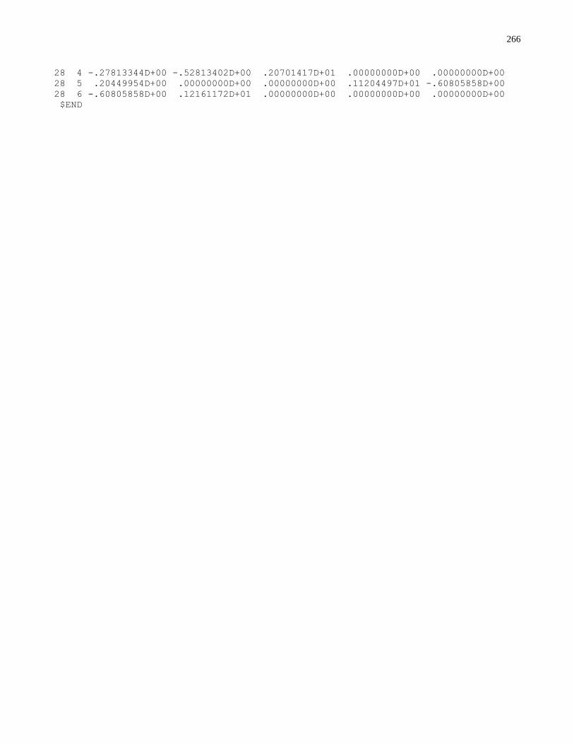
266

28 4 -.27813344D+00 -.52813402D+00 .20701417D+01 .00000000D+00 .00000000D+00

28 5 .20449954D+00 .00000000D+00 .00000000D+00 .11204497D+01 -.60805858D+00

28 6 -.60805858D+00 .12161172D+01 .00000000D+00 .00000000D+00 .00000000D+00

$END

267

SAMPLE 21: MC-QDPT2 calculation

A second example of MC-QDPT2 calculation follows.

Input

$CNTRL RUNFLG=0, NOPROP=1, NOSYM=0, TIME=3500.0, $END



$MCQDPT NSTATE=2, NSTCI=2, KSTATE=1,1, $END



ISTSYM=1, NSTATE=2, NSTCI=2, KSTATE=1,1,

INORB=0, IFORB=1, $END

$DRT

LiF,1A1,MCSCF

0 9 1 6

3*FZC 3*DOC 3*VAL

$END

$MC MAXIT=50 $END

$GUGDIA NSTATE=2, MAXIT=200, $END

$GUGDM2 NSTATE=2, ISTATE=1,2, WSTATE=1.0,1.0, $END

$BASIS

LIF

0 0 0 -1 .... ....

CNV 2

LIT 3. 0. 0. 0.

1 S 5

1 921.3 0.001367

2 138.7 0.010425

3 31.94 0.049859

4 9.353 0.160701

5 3.158 0.344604

2 S 2

1 1.157 0.425197

2 0.4446 0.169468

3 S 1

1 0.07666 1.0

4 S 1

1 0.02864 1.0

5 P 3

1 1.488 0.038770

2 0.2667 0.236257

3 0.07201 0.830448

6 P 1

1 0.02370 1.0

FLU 9. 0.00 0.00 9.5

1 S 6

1 9994.79 0.002017

2 1506.03 0.015295

3 350.269 0.073110

4 104.053 0.246420

5 34.8432 0.612593

268

6 4.3688 0.242489

2 S 1

1 12.2164 1.0

3 S 1

1 1.2078 1.0

4 S 1

1 0.3634 1.0

5 P 4

1 44.3555 0.020868

2 10.0820 0.130092

3 2.9959 0.396219

4 0.9383 0.620368

6 P 1

1 0.2733 1.0

7 P 1

1 0.08 1.0

8 D 1

1 1.4 1.0

$END

$VEC

1 1 -.11351214E-05 .96924794E-06 -.66866347E-05 .13813057E-04 -.23148014E-15

1 2 .19237446E-15 -.73563688E-05 .16476311E-15 .13927527E-15 .14995238E-04

1 3 -.57996267E+00 -.46252777E+00 .10596238E-02 -.77050371E-03 -.65774721E-16

1 4 -.64100802E-16 .12598879E-04 .18943287E-15 .18777246E-15 -.15507484E-04

1 5 -.20502582E-15 -.20848285E-15 .89575136E-05 -.65855197E-03 -.65855193E-03

1 6 -.45842255E-03 .21795887E-11 .13919069E-15 .55521751E-15

2 1 -.51707512E+00 -.57519806E+00 -.14745022E-02 .69146833E-04 -.51018951E-15

2 2 .40398490E-15 .49388920E-03 .36945365E-15 .34396670E-15 -.24374918E-03

2 3 -.57217398E-06 -.22338174E-05 -.59632160E-05 .45272155E-04 -.13168700E-15

2 4 -.13940022E-15 .68032939E-05 .38027807E-15 .41352305E-15 -.18410983E-05

2 5 -.41432807E-15 -.46649505E-15 -.12625702E-04 -.75226855E-05 -.75226710E-05

2 6 -.75259761E-05 -.32998664E-13 .23860819E-15 .10364796E-15

…

orbitals 3-27 not shown here

…

28 1 .13336536E-01 -.20127815E-01 .48869636E-01 -.54817211E-01 .95943059E-15

28 2 -.93775325E-15 .32732240E-01 -.65468193E-15 -.43364697E-15 -.67476141E-01

28 3 -.22200891E+00 -.52677957E+00 .18080292E+01 .13022500E+01 .30516526E-15

28 4 .27787788E-15 -.39193361E-02 -.87206565E-15 -.81397304E-15 .13419983E-01

28 5 .93183587E-15 .89591635E-15 -.27725569E-01 -.13166698E+01 -.13166698E+01

28 6 -.13116400E+01 .21936147E-10 -.18563298E-14 -.96111656E-15

29 1 -.11279401E-02 .26265554E-02 -.11359510E-01 .13434714E-01 .22674892E-15

29 2 -.19321700E-15 -.86578888E-02 -.16066211E-15 -.13022302E-15 .17707727E-01

29 3 -.17549381E+01 .21063583E+01 -.79651895E+00 -.32407697E+00 .66712551E-16

29 4 .63500349E-16 .74042927E-03 -.19170399E-15 -.18725733E-15 -.30317669E-02

29 5 .20675575E-15 .20883908E-15 .69438593E-02 .41255053E+00 .41255053E+00

29 6 .41251304E+00 .28792883E-12 -.22559948E-15 -.11677240E-15

$END

269

SAMPLE 21-1: MC-QDPT2 calculation of SAMPLE 21 with EDSHFT=0.02 (ISA method)

Input

$CNTRL RUNFLG=0, NOPROP=1, NOSYM=0, TIME=3500.0, $END





ISTSYM=1, NSTATE=2, NSTCI=2, KSTATE=1,1,

INORB=0, IFORB=1, EDSHFT=0.02 $END

$DRT

LiF,1A1,MCSCF

0 9 1 6

3*FZC 3*DOC 3*VAL

$END

$MC MAXIT=50 $END

$GUGDIA NSTATE=2, MAXIT=200, $END

$GUGDM2 NSTATE=2, ISTATE=1,2, WSTATE=1.0,1.0, $END

$BASIS

LIF

0 0 0 -1 .... ....

CNV 2

LIT 3. 0. 0. 0.

1 S 5

1 921.3 0.001367

2 138.7 0.010425

3 31.94 0.049859

4 9.353 0.160701

5 3.158 0.344604

2 S 2

1 1.157 0.425197

2 0.4446 0.169468

3 S 1

1 0.07666 1.0

4 S 1

1 0.02864 1.0

5 P 3

1 1.488 0.038770

2 0.2667 0.236257

3 0.07201 0.830448

6 P 1

1 0.02370 1.0

FLU 9. 0.00 0.00 9.5

1 S 6

1 9994.79 0.002017

2 1506.03 0.015295

3 350.269 0.073110

4 104.053 0.246420

5 34.8432 0.612593

6 4.3688 0.242489

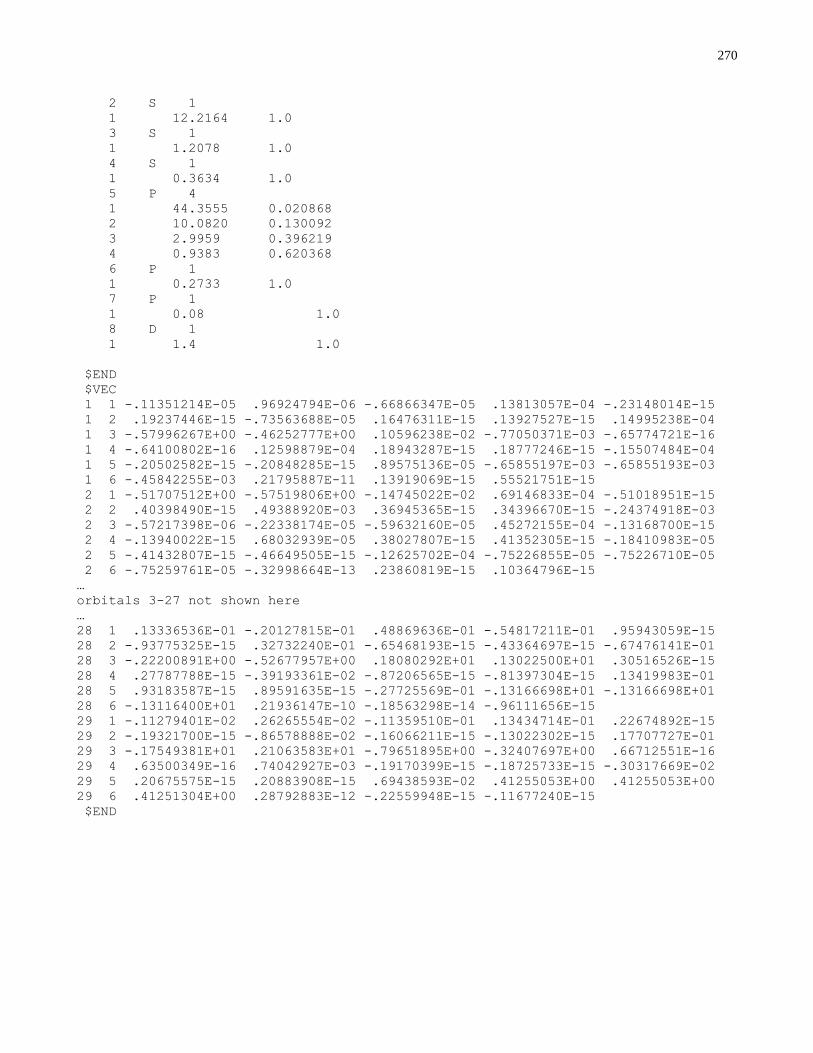
270

2 S 1

1 12.2164 1.0

3 S 1

1 1.2078 1.0

4 S 1

1 0.3634 1.0

5 P 4

1 44.3555 0.020868

2 10.0820 0.130092

3 2.9959 0.396219

4 0.9383 0.620368

6 P 1

1 0.2733 1.0

7 P 1

1 0.08 1.0

8 D 1

1 1.4 1.0

$END

$VEC

1 1 -.11351214E-05 .96924794E-06 -.66866347E-05 .13813057E-04 -.23148014E-15

1 2 .19237446E-15 -.73563688E-05 .16476311E-15 .13927527E-15 .14995238E-04

1 3 -.57996267E+00 -.46252777E+00 .10596238E-02 -.77050371E-03 -.65774721E-16

1 4 -.64100802E-16 .12598879E-04 .18943287E-15 .18777246E-15 -.15507484E-04

1 5 -.20502582E-15 -.20848285E-15 .89575136E-05 -.65855197E-03 -.65855193E-03

1 6 -.45842255E-03 .21795887E-11 .13919069E-15 .55521751E-15

2 1 -.51707512E+00 -.57519806E+00 -.14745022E-02 .69146833E-04 -.51018951E-15

2 2 .40398490E-15 .49388920E-03 .36945365E-15 .34396670E-15 -.24374918E-03

2 3 -.57217398E-06 -.22338174E-05 -.59632160E-05 .45272155E-04 -.13168700E-15

2 4 -.13940022E-15 .68032939E-05 .38027807E-15 .41352305E-15 -.18410983E-05

2 5 -.41432807E-15 -.46649505E-15 -.12625702E-04 -.75226855E-05 -.75226710E-05

2 6 -.75259761E-05 -.32998664E-13 .23860819E-15 .10364796E-15

…

orbitals 3-27 not shown here

…

28 1 .13336536E-01 -.20127815E-01 .48869636E-01 -.54817211E-01 .95943059E-15

28 2 -.93775325E-15 .32732240E-01 -.65468193E-15 -.43364697E-15 -.67476141E-01

28 3 -.22200891E+00 -.52677957E+00 .18080292E+01 .13022500E+01 .30516526E-15

28 4 .27787788E-15 -.39193361E-02 -.87206565E-15 -.81397304E-15 .13419983E-01

28 5 .93183587E-15 .89591635E-15 -.27725569E-01 -.13166698E+01 -.13166698E+01

28 6 -.13116400E+01 .21936147E-10 -.18563298E-14 -.96111656E-15

29 1 -.11279401E-02 .26265554E-02 -.11359510E-01 .13434714E-01 .22674892E-15

29 2 -.19321700E-15 -.86578888E-02 -.16066211E-15 -.13022302E-15 .17707727E-01

29 3 -.17549381E+01 .21063583E+01 -.79651895E+00 -.32407697E+00 .66712551E-16

29 4 .63500349E-16 .74042927E-03 -.19170399E-15 -.18725733E-15 -.30317669E-02

29 5 .20675575E-15 .20883908E-15 .69438593E-02 .41255053E+00 .41255053E+00

29 6 .41251304E+00 .28792883E-12 -.22559948E-15 -.11677240E-15

$END

271

SAMPLE 22: Molecular Dynamics calculation

Example of molecular dynamics run.

Input

$FIL FILSAV=1, $END

$CNTRL IREST=0, RUNFLG=13, NOPROP=0, $END

$DYN IREST=0, NSTEP=12, NSAVE=5, $END

$BASINP IUNIT=-1, $END

$GEO

water dimer

O1 0.0000 0.0000 0.0000

H11 1.1072 1.4304 0.0000

H12 1.1072 -1.4304 0.0000

O2 -4.4006 1.8228 2.7500

H21 -5.8685 1.6789 1.7029

H22 -3.1075 0.9426 1.8415

$END

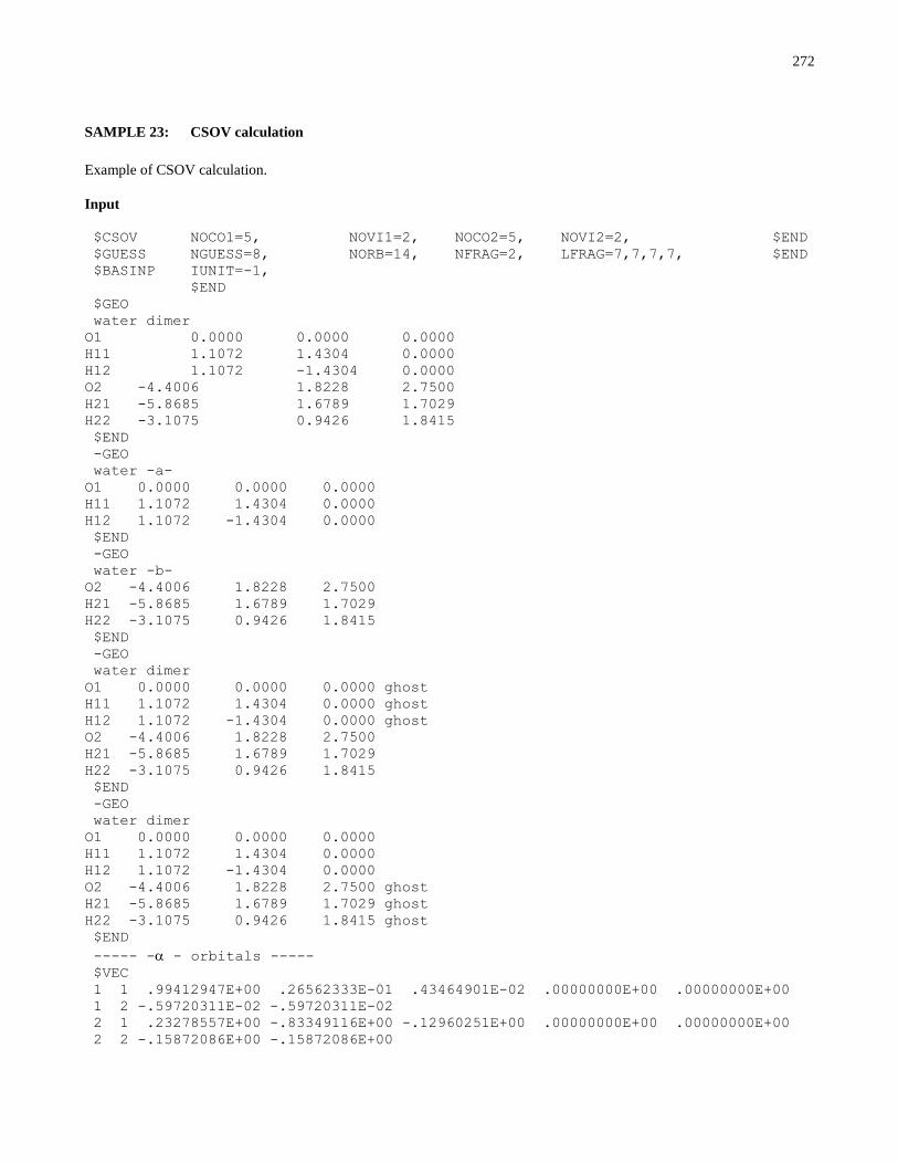
272

SAMPLE 23: CSOV calculation

Example of CSOV calculation.

Input

$CSOV NOCO1=5, NOVI1=2, NOCO2=5, NOVI2=2, $END

$GUESS NGUESS=8, NORB=14, NFRAG=2, LFRAG=7,7,7,7, $END

$BASINP IUNIT=-1,

$END

$GEO

water dimer

O1 0.0000 0.0000 0.0000

H11 1.1072 1.4304 0.0000

H12 1.1072 -1.4304 0.0000

O2 -4.4006 1.8228 2.7500

H21 -5.8685 1.6789 1.7029

H22 -3.1075 0.9426 1.8415

$END

-GEO

water -a-

O1 0.0000 0.0000 0.0000

H11 1.1072 1.4304 0.0000

H12 1.1072 -1.4304 0.0000

$END

-GEO

water -b-

O2 -4.4006 1.8228 2.7500

H21 -5.8685 1.6789 1.7029

H22 -3.1075 0.9426 1.8415

$END

-GEO

water dimer

O1 0.0000 0.0000 0.0000 ghost

H11 1.1072 1.4304 0.0000 ghost

H12 1.1072 -1.4304 0.0000 ghost

O2 -4.4006 1.8228 2.7500

H21 -5.8685 1.6789 1.7029

H22 -3.1075 0.9426 1.8415

$END

-GEO

water dimer

O1 0.0000 0.0000 0.0000

H11 1.1072 1.4304 0.0000

H12 1.1072 -1.4304 0.0000

O2 -4.4006 1.8228 2.7500 ghost

H21 -5.8685 1.6789 1.7029 ghost

H22 -3.1075 0.9426 1.8415 ghost

$END

----- - - orbitals -----

$VEC

1 1 .99412947E+00 .26562333E-01 .43464901E-02 .00000000E+00 .00000000E+00

1 2 -.59720311E-02 -.59720311E-02

2 1 .23278557E+00 -.83349116E+00 -.12960251E+00 .00000000E+00 .00000000E+00

2 2 -.15872086E+00 -.15872086E+00

273

3 1 .00000000E+00 .00000000E+00 .00000000E+00 -.60644807E+00 .00000000E+00

3 2 -.44500310E+00 .44500310E+00

4 1 .10317796E+00 -.53687077E+00 .77673374E+00 .00000000E+00 .00000000E+00

4 2 .27783171E+00 .27783171E+00

5 1 .00000000E+00 .00000000E+00 .00000000E+00 .00000000E+00 .10000000E+01

5 2 .00000000E+00 .00000000E+00

6 1 -.13238973E+00 .88475179E+00 .74233232E+00 .00000000E+00 .00000000E+00

6 2 -.79715745E+00 -.79715745E+00

7 1 .00000000E+00 .00000000E+00 .00000000E+00 .99059266E+00 .00000000E+00

7 2 -.83869998E+00 .83869998E+00

$END

----- -- orbitals ----- $VEC

1 1 -.99412951E+00 -.26561999E-01 .34362375E-03 .20098869E-02 .38383395E-02

1 2 .59722289E-02 .59714811E-02

2 1 .23278620E+00 -.83349701E+00 .10249322E-01 .59928975E-01 .11444996E+00

2 2 -.15873055E+00 -.15870912E+00

3 1 .88332809E-05 -.48263322E-04 -.58528370E+00 .15606379E+00 -.29415187E-01

3 2 .44500426E+00 -.44500383E+00

4 1 -.10317701E+00 .53686508E+00 .61323768E-01 .35920888E+00 .68594403E+00

4 2 -.27781999E+00 -.27785565E+00

5 1 .00000000E+00 .00000000E+00 -.24969359E+00 -.84846875E+00 .46664107E+00

5 2 .00000000E+00 .00000000E+00

6 1 .13238758E+00 -.88472449E+00 .58424743E-01 .34334869E+00 .65555506E+00

6 2 .79698557E+00 .79730661E+00

7 1 .32824939E-04 -.24337413E-03 .95602552E+00 -.25485772E+00 .48162567E-01

7 2 .83888085E+00 -.83848970E+00

$END

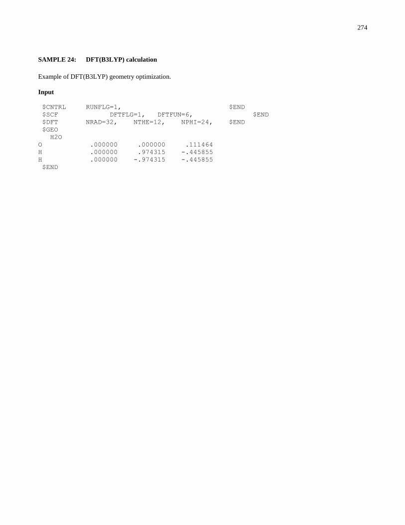
274

SAMPLE 24: DFT(B3LYP) calculation

Example of DFT(B3LYP) geometry optimization.

Input


$SCF DFTFLG=1, DFTFUN=6, $END

$DFT NRAD=32, NTHE=12, NPHI=24, $END

$GEO

H2O

O .000000 .000000 .111464

H .000000 .974315 -.445855

H .000000 -.974315 -.445855

$END

275

SAMPLE 25: Finite-Field 2D NLO calculation

This is an example of finite-field NLO calculation using the 2D code.

Input


$NLO IF2D=1, $END

$BASIS

HF TEST CALCULATION FOR (HYPER)POLARIZABILY

0 0 15 1 ... ...

C1 1

H 1. 0.0 0.0 -0.45855

1 S 3

1 19.2406 0.032828

2 2.8992 0.231208

3 0.6534 0.817238

2 S 1

1 0.1776 1.0

F 9. 0.0 0.0 0.45855

1 S 6

1 9994.79 0.002017

2 1506.03 0.015295

3 350.269 0.073110

4 104.0530 0.246420

5 34.8432 0.612593

6 4.3688 0.242489

2 S 1

1 12.2164 1.0

3 S 1

1 1.2078 1.0

4 S 1

1 0.3634 1.0

5 P 4

1 44.3555 0.020868

2 10.0820 0.130092

3 2.9959 0.396219

4 0.9383 0.620368

6 P 1

1 0.2733 1.0

$END

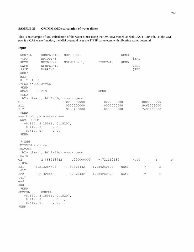
276

SAMPLE 26: QM/MM (MD) calculation of water dimer

This is an example of MD calculation of the water dimer using the QM/MM model labeled CAS/TIP3P-vib, i.e. the QM

part is a CAS wave function, the MM potential uses the TIP3P parameters with vibrating water potential.

Input


$OPT NPTOPT=1, $END

$DYN NPTDYN=2, NORMKE = 1, IFOPT=1, $END

$WFN WFNFLG=1, $END

$SCF MOPRT=7, $END

$DRT

H2O

0 7 1 8

1*FZC 4*DOC 2*VAL

$END

$BAS 3-21G $END

$GEO

h2o dimer , hf 6-31g* -opt- geom

O1 .0000000000 .0000000000 .0000000000

H11 .0000000000 .0000000000 .9463209000

H12 .9180483000 .0000000000 -.2495168000

$END

--- tip3p parameters ---

$QM QSEQM=

-0.834, 3.15066, 0.15207,

0.417, 0. , 0.

0.417, 0. , 0.

$END

$QMMM

!BIOSYM archive 3

PBC=OFF


!DATE

O2 2.888518942 .000000000 -.721112135 wat0 ? O

-.834

H21 3.213284403 -.757378442 -1.189260823 wat0 ? H

.417

H22 3.213284403 .757378442 -1.189260823 wat0 ? H

.417

end

end

$END

$MMPOL QSEMM=

-0.834, 3.15066, 0.15207,

0.417, 0. , 0. ,

0.417, 0. , 0. ,

$END

277

SAMPLE 26-1: QM/MM (MD) calculation of water dimer with a non-polarizable solvent (water)

This test case illustrates the use of the newly named $MMNOPOL namelist.

Input


$OPT NPTOPT=1, $END

$DYN NPTDYN=2, NORMKE = 1, IFOPT=1, $END

$WFN WFNFLG=1, $END

$SCF MOPRT=7, $END

$DRT

H2O

0 7 1 8

1*FZC 4*DOC 2*VAL

$END

$BAS 3-21G $END

$GEO


O1 .0000000000 .0000000000 .0000000000

H11 .0000000000 .0000000000 .9463209000

H12 .9180483000 .0000000000 -.2495168000

$END

--- tip3p parameters ---

$QM QSEQM=

-0.834, 3.15066, 0.15207,

0.417, 0. , 0.

0.417, 0. , 0.

$END

$QMMM

!BIOSYM archive 3

PBC=OFF


!DATE

O2 2.888518942 .000000000 -.721112135 wat0 ? O

-.834

H21 3.213284403 -.757378442 -1.189260823 wat0 ? H

.417

H22 3.213284403 .757378442 -1.189260823 wat0 ? H

.417

end

end

$END

$MMNOPOL QSEMM=

-0.834, 3.15066, 0.15207,

0.417, 0. , 0. ,

0.417, 0. , 0. ,

$END

278

SAMPLE 27: COSMO calculation---DISCONTINUED

Input

$CNTRL RUNFLG=1 , $END

$OPT NPTOPT=1, $END

$COSMO MINBEM=2, MAXBEM=4,

RADIUS=1.40, 1.16, 1.16, RSOLV=0.0, $END

$WFN WFNFLG=1, $END

$SCF MAXIT=20, MOPRT=0, UHFFLG=0, DFTFLG=0, NPFLG=0, $END

$DRT

H2O

0 7 1 8

1*FZC 4*DOC 2*VAL

$END

$BAS 6-31G $END

$GEO

H2O 6-31G* HF -opt- geom

O .0000000000 .0000000000 -.0486020332

H .7545655371 .0000000000 .5243010666

H -.7545655371 .0000000000 .5243010666

$END

SAMPLE 28: HF/6-31G(d) optimization of water with the H-O-H angle frozen

This test case illustrates how the $GEO data group can be used to specify frozen coordinates. The program will

automatically generate the $FREZ namelist, which is used to let the program know which coordinates are frozen.

Input


$OPT CVGOPT=0.0001 $END

$BAS 6-31G* $END

$GEO

‘Geometry optimization of water at the HF/6-31G(d,p) level of theory’

O

H 1 R21

H 1 R21 2 A321

R21=1.0

A321=110.0

$END

279

SAMPLE S1: SM6/mPW1PW91/MIDI!6D single-point calculation of water dimer in water.

Input

$SCF DFTFLG=1 DFTFUN=3250 $END

$CNTRL ISPHER=0 $END

$BAS MIDIX $END

$GEO

SM6/mPW1PW91/MIDIX6D single-point for water dimer

O -.000801 -1.400129 .000000

H .502095 -1.695193 .763233

H .502095 -1.695193 -.763233

H -.093294 .558870 .000000

O -.000801 1.521654 .000000

H -.898077 1.859309 .000000

$END

$HONDOS ISCRF=1 ICMD=416 HFE=0.25 $END

Results

Summary of SM6 solvation calculation by HONDOPLUS-v5.2

--------------------------------------------------------------------------------

Options: ISCRF = 1, IGAS = 0, ICMD =416, ICDS =416, IAQU = 1, DIELEC = 78.30

(0) E-EN(g) gas-phase elect-nuc energy -151.936649139 a.u.

(1) E-EN(liq) elect-nuc energy of solute -151.935696040 a.u.

(2) G-P(liq) polarization free energy of solvation -9.766 kcal/mol

(3) G-ENP(liq) elect-nuc-pol free energy of system -151.951259308 a.u.

(4) G-CDS(liq) cavity-dispersion-solvent structure

free energy -6.473 kcal/mol

(5) G-P-CDS(liq) = G-P(liq) + G-CDS(liq) = (2) + (4) -16.239 kcal/mol

(6) G-S(liq) free energy of system = (1) + (5) -151.961574965 a.u.

(7) DeltaE-EN(liq) elect-nuc reorganization

energy of solute molecule (7) = (1) - (0) .598 kcal/mol

(8) DeltaG-ENP(liq) elect-nuc-pol free energy

of solvation (8) = (3) - (0) -9.168 kcal/mol

(9) DeltaG-S(liq) free energy of solvation

(9) = (6) - (0) -15.641 kcal/mol

--------------------------------------------------------------------------------

280

SAMPLE S2: SM6/B3LYP/6-31G* geometry optimization of water in water

Input

$SCF DFTFLG=1 DFTFUN=6 $END

$CNTRL RUNFLG=1 $END

$BAS 6-31G* $END

$GEO

SM6/B3LYP/6-31G* geometry optimization of water

O -.000801 -1.400129 .000000

H .502095 -1.695193 .763233

H .502095 -1.695193 -.763233

$END

$HONDOS ISCRF=1 ICMD=417 HFE=0.200 $END

Results

Summary of SM6 solvation calculation by HONDOPLUS-v5.2

--------------------------------------------------------------------------------















(9) = (6) - (0) -9.090 kcal/mol

LARGEST COMPONENT OF GRADIENT .0003044 ( CVGOPT = .0005000 )

INTERNUCLEAR DISTANCES (ANGS.)

------------------------------

O H H

1 O .0000000 .9741788 .9741788

2 H .9741788 .0000000 1.5076518

3 H .9741788 1.5076518 .0000000

281

SAMPLE S3: SM5.43/HF/6-31G* liquid-phase gradient calculation for HF in ethyl acetate

Input

$SCF NOSLZ=1 DAMP=0.0 MOPRT=0

MAXIT=100 ACURCY=0.00001

$END

$CNTRL RUNFLG=-3 NOPROP=1 ISPHER=0 $END

$BAS 6-31G* $END

$GEO

Liquid-phase Gradient for HF in ethyl acetate

F

H F HF

HF=0.92489165

$END

$HONDOS ISCRF=1 ICMD=303 IAQU=0 DIELEC=5.99 SOLN=1.3723

SOLA=0.00 SOLB=0.45 SOLG=33.67 SOLC=0.00 SOLH=0.00 $END

Results:

Summary of SM5.43 solvation calculation by HONDOPLUS-v5.2

--------------------------------------------------------------------------------















(9) = (6) - (0) -7.681 kcal/mol

--------------------------------------------------------------------------------

282

SAMPLE S4 Diabatization of HNCO(S0,S1) based on CASSCF (Threefold density criterion)

&CNTRL RUNFLG=0, NOPROP=1, NOSYM=1, TIME=35000.0, &END

&GUESS NGUESS=5,

NORB=50, $END

&WFN WFNFLG=15, &END

$DRT

HNCO (Cs geometry but not Cs constrained) active=H(s)N(sp)C(sp)O(p)

0 15 1 8

5*MCC 6*DOC 4*VAL

$END

$MC ACURCY=.1E-04 MAXIT=50 ,$END

&GUGDIA NSTATE=2, MAXIT=100, &END

&GUGDM2 NSTATE=2, ISTATE=1,2, WSTATE=1.0,1.0 &END

$MCQDPT NEL=22, MULT=1, NMOFZC=3,NMODOC=2, NMOACT=10, NMOEXT=35

NSTATE=2, INORB=0, NSTCI=2, KSTATE=1,1, IFORB=0, $END

&DIABAT NDMOSYM=0, NRCSF=1, NDFRM=1 $END

&PROTOTYPE NMLAP=0 $END

$BASIS

HNCO

0 0 0 -1 .... ....

C1

HYD 1.0 .6840 1.8794 .0000

1 S 3

1 13.0100000 0.0196850000

2 1.9620000 0.1379770000

3 0.4446000 0.4781480000

2 S 1

1 0.1220000 1.0000000000

3 P 1

1 0.7270000 1.0000000000

NIT 7.0 .0000 .0000 .0000

1 S 8

1 9046.0000000 0.0007000000

2 1357.0000000 0.0053890000

3 309.3000000 0.0274060000

4 87.7300000 0.1032070000

5 28.5600000 0.2787230000

6 10.2100000 0.4485400000

7 3.8380000 0.2782380000

8 0.7466000 0.0154400000

2 S 8

1 9046.0000000 -0.0001530000

2 1357.0000000 -0.0012080000

3 309.3000000 -0.0059920000

4 87.7300000 -0.0245440000

5 28.5600000 -0.0674590000

6 10.2100000 -0.1580780000

7 3.8380000 -0.1218310000

8 0.7466000 0.5490030000

3 S 1

283

1 0.2248000 1.0000000000

4 P 3

1 13.5500000 0.0399190000

2 2.9170000 0.2171690000

3 0.7973000 0.5103190000

5 P 1

1 0.2185000 1.0000000000

6 D 1

1 0.8170000 1.0000000000

CAR 6.0 -2.5000 .0000 .0000

1 S 8

1 6665.0000000 0.0006920000

2 1000.0000000 0.0053290000

3 228.0000000 0.0270770000

4 64.7100000 0.1017180000

5 21.0600000 0.2747400000

6 7.4950000 0.4485640000

7 2.7970000 0.2850740000

8 0.5215000 0.0152040000

2 S 8

1 6665.0000000 -0.0014600000

2 1000.0000000 -0.0011540000

3 228.0000000 -0.0057250000

4 64.7100000 -0.0233120000

5 21.0600000 -0.0639550000

6 7.4950000 -0.1499810000

7 2.7970000 -0.1272620000

8 0.5215000 0.5445290000

3 S 1

1 0.1596000 1.0000000000

4 P 3

1 9.4390000 0.0381090000

2 2.0020000 0.2094800000

3 0.5456000 0.5085570000

5 P 1

1 0.1517000 1.0000000000

6 D 1

1 0.5500000 1.0000000000

OXY 8.0 -4.4486 -1.1250 .0000

1 S 8

1 11720.0000000 0.0007100000

2 1759.0000000 0.0054700000

3 400.8000000 0.0278370000

4 113.7000000 0.1048000000

5 37.0300000 0.2830620000

6 13.2700000 0.4487190000

7 5.0250000 0.2709520000

8 1.0130000 0.0154580000

2 S 8

1 11720.0000000 -0.0001600000

2 1759.0000000 -0.0012630000

3 400.8000000 -0.0062670000

4 113.7000000 -0.0257160000

5 37.0300000 -0.0709240000

6 13.2700000 -0.1654110000

284

7 5.0250000 -0.1169550000

8 1.0130000 0.5573680000

3 S 1

1 0.3023000 1.0000000000

4 P 3

1 17.7000000 0.0430180000

2 3.8540000 0.2289130000

3 1.0460000 0.5087280000

5 P 1

1 0.2753000 1.0000000000

6 D 1

1 1.1850000 1.0000000000

$END

...

$DFMVEC and $VEC are not shown here. See the sample file.

…

285

SAMPLE S5 Diabatization of HNCO(S0,S1) based on CASSCF (Fourfold way with one reference MO)


&GUESS NGUESS=5,

NORB=50, $END


$DRT


0 15 1 8

5*MCC 6*DOC 4*VAL

$END






&DIABAT NDMOSYM=0, NRCSF=1, NDFRM=1,th_doc=1.8, th_vir=0.3,

MOSLAB_CHARACT=1,1,1,1,1,1,1,1,1,1, $END


$BASIS

…………not shown here, because same with sample S4

$END

------ Reference orbitals (modified as N(pz) alpne)----

$CSFDAT

4

2437( 1)

8066( 1)

13735( 1)

8065( 2)

1 1 -.93668614E+00 -.10565065E+00 .54533763E-02 -.21920916E-08

2 1 -.21448374E-07 .17068897E-06 .17168341E-08 -.93236749E+00

$END

$DIAVEC

1 1 .00000000E+00 .00000000E+00 .00000000E+00 .00000000E+00 .26527331E-01

1 2 .00000000E+00 .00000000E+00 .00000000E+00 .00000000E+00 .00000000E+00

1 3 .63824278E+00 .00000000E+00 .00000000E+00 .49530013E+00 .00000000E+00

1 4 .00000000E+00 .00000000E+00 .00000000E+00 .00000000E+00 .20194524E-01

1 5 .00000000E+00 .00000000E+00 .00000000E+00 .00000000E+00 .00000000E+00

1 6 .00000000E+00 .00000000E+00 .00000000E+00 .00000000E+00 .00000000E+00

1 7 .00000000E+00 .00000000E+00 .00000000E+00 .00000000E+00 .00000000E+00

1 8 .00000000E+00 .00000000E+00 .00000000E+00 .00000000E+00 .00000000E+00

1 9 .00000000E+00 .00000000E+00 .00000000E+00 .00000000E+00 .00000000E+00

1 10 .00000000E+00 .00000000E+00 .00000000E+00 .00000000E+00 .00000000E+00

$END

...


…

286

SAMPLE S6 Diabatization of HNCO(S0,S1) based on CASSCF

(Fourfold way with one reference MO and use of DC, VL, and VIR blocks)


&GUESS NGUESS=5,

NORB=50, $END


$DRT


0 15 1 8

5*MCC 6*DOC 4*VAL

$END







MOSLAB_CHARACT=2,2,2,2,1,1,1,0,0,0, $END


$BASIS

…………not shown here, because same with sample S4

$END

$CSFDAT

4

2437( 1)

8066( 1)

13735( 1)

8065( 2)

1 1 -.93668614E+00 -.10565065E+00 .54533763E-02 -.21920916E-08

2 1 -.21448374E-07 .17068897E-06 .17168341E-08 -.93236749E+00

$END

------ Diabatic orbitals (modified as N(pz) alpne)----

$DIAVEC

1 1 .00000000E+00 .00000000E+00 .00000000E+00 .00000000E+00 .26527331E-01

1 2 .00000000E+00 .00000000E+00 .00000000E+00 .00000000E+00 .00000000E+00

1 3 .63824278E+00 .00000000E+00 .00000000E+00 .49530013E+00 .00000000E+00

1 4 .00000000E+00 .00000000E+00 .00000000E+00 .00000000E+00 .20194524E-01

1 5 .00000000E+00 .00000000E+00 .00000000E+00 .00000000E+00 .00000000E+00

1 6 .00000000E+00 .00000000E+00 .00000000E+00 .00000000E+00 .00000000E+00

1 7 .00000000E+00 .00000000E+00 .00000000E+00 .00000000E+00 .00000000E+00

1 8 .00000000E+00 .00000000E+00 .00000000E+00 .00000000E+00 .00000000E+00

1 9 .00000000E+00 .00000000E+00 .00000000E+00 .00000000E+00 .00000000E+00

1 10 .00000000E+00 .00000000E+00 .00000000E+00 .00000000E+00 .00000000E+00

$END

...


…

287

SAMPLE S7 Diabatization of HNCO(S0,S1) based on MC-QDPT

(Fourfold way with one reference MO, use of DC, VL, and VIR blocks, three resolution MOs for the DC block, and

specific orientations for the reference and resolution MOs)


&GUESS NGUESS=5,

NORB=50, $END


$DRT

HNCO active=H(s)N(sp)C(sp)O(p)

0 15 1 8

5*MCC 6*DOC 4*VAL

$END







MOSLAB_CHARACT=2,2,2,2,1,1,1,0,0,0, conv_th=0.00001

max_iter=2000 $END

&PROTOTYPE NMLAP=1 NDLAP=3, NORIENT=1, $END

$BASIS

HNCO

0 0 0 -1 .... ....

C1

HYD 1.0 .6840 1.8794 .0000

1 S 3

1 13.0100000 0.0196850000

2 1.9620000 0.1379770000

3 0.4446000 0.4781480000

2 S 1

1 0.1220000 1.0000000000

3 P 1

1 0.7270000 1.0000000000

NIT 7.0 .0000 .0000 .0000

1 S 8

1 9046.0000000 0.0007000000

2 1357.0000000 0.0053890000

3 309.3000000 0.0274060000

4 87.7300000 0.1032070000

5 28.5600000 0.2787230000

6 10.2100000 0.4485400000

7 3.8380000 0.2782380000

8 0.7466000 0.0154400000

2 S 8

1 9046.0000000 -0.0001530000

2 1357.0000000 -0.0012080000

3 309.3000000 -0.0059920000

4 87.7300000 -0.0245440000

5 28.5600000 -0.0674590000

6 10.2100000 -0.1580780000

288

7 3.8380000 -0.1218310000

8 0.7466000 0.5490030000

3 S 1

1 0.2248000 1.0000000000

4 P 3

1 13.5500000 0.0399190000

2 2.9170000 0.2171690000

3 0.7973000 0.5103190000

5 P 1

1 0.2185000 1.0000000000

6 D 1

1 0.8170000 1.0000000000

CAR 6.0 -3.1000 .0000 .0000

1 S 8

1 6665.0000000 0.0006920000

2 1000.0000000 0.0053290000

3 228.0000000 0.0270770000

4 64.7100000 0.1017180000

5 21.0600000 0.2747400000

6 7.4950000 0.4485640000

7 2.7970000 0.2850740000

8 0.5215000 0.0152040000

2 S 8

1 6665.0000000 -0.0014600000

2 1000.0000000 -0.0011540000

3 228.0000000 -0.0057250000

4 64.7100000 -0.0233120000

5 21.0600000 -0.0639550000

6 7.4950000 -0.1499810000

7 2.7970000 -0.1272620000

8 0.5215000 0.5445290000

3 S 1

1 0.1596000 1.0000000000

4 P 3

1 9.4390000 0.0381090000

2 2.0020000 0.2094800000

3 0.5456000 0.5085570000

5 P 1

1 0.1517000 1.0000000000

6 D 1

1 0.5500000 1.0000000000

OXY 8.0 -3.4907 -2.2074 .1931

1 S 8

1 11720.0000000 0.0007100000

2 1759.0000000 0.0054700000

3 400.8000000 0.0278370000

4 113.7000000 0.1048000000

5 37.0300000 0.2830620000

6 13.2700000 0.4487190000

7 5.0250000 0.2709520000

8 1.0130000 0.0154580000

2 S 8

1 11720.0000000 -0.0001600000

2 1759.0000000 -0.0012630000

3 400.8000000 -0.0062670000

289

4 113.7000000 -0.0257160000

5 37.0300000 -0.0709240000

6 13.2700000 -0.1654110000

7 5.0250000 -0.1169550000

8 1.0130000 0.5573680000

3 S 1

1 0.3023000 1.0000000000

4 P 3

1 17.7000000 0.0430180000

2 3.8540000 0.2289130000

3 1.0460000 0.5087280000

5 P 1

1 0.2753000 1.0000000000

6 D 1

1 1.1850000 1.0000000000

$END

!--- Info of resolution MOs ---

-- (1) At ref geometry (HN---CO colinear), 3fold. C(S):

--remove other components

---(2) CO (pi): remove components smaller than 0.1

---(3) N(S): remove other components

$DPSVEC -- CO(pi) N(s) C(s)

1 1 .00000000E+00 .00000000E+00 .00000000E+00 .00000000E+00 .00000000E+00

1 2 .00000000E+00 .00000000E+00 .00000000E+00 .00000000E+00 .00000000E+00

1 3 .00000000E+00 .00000000E+00 .00000000E+00 .00000000E+00 .00000000E+00

1 4 .00000000E+00 .00000000E+00 .00000000E+00 .00000000E+00 .00000000E+00

1 5 .00000000E+00 .00000000E+00 .00000000E+00 .00000000E+00 .32175892E+00

1 6 .00000000E+00 .00000000E+00 .14154391E+00 .00000000E+00 .00000000E+00

1 7 .00000000E+00 .00000000E+00 .00000000E+00 .00000000E+00 .00000000E+00

1 8 .00000000E+00 .00000000E+00 .00000000E+00 .00000000E+00 .54870384E+00

1 9 .00000000E+00 .00000000E+00 .33021457E+00 .00000000E+00 .00000000E+00

1 10 .00000000E+00 .00000000E+00 .00000000E+00 .00000000E+00 .00000000E+00

2 1 .00000000E+00 .00000000E+00 .00000000E+00 .00000000E+00 .00000000E+00

2 2 .00000000E+00 .47720417E+00 .57390110E+00 .00000000E+00 .00000000E+00

2 3 .00000000E+00 .00000000E+00 .00000000E+00 .00000000E+00 .00000000E+00

2 4 .00000000E+00 .00000000E+00 .00000000E+00 .00000000E+00 .00000000E+00

2 5 .00000000E+00 .00000000E+00 .00000000E+00 .00000000E+00 .00000000E+00

2 6 .00000000E+00 .00000000E+00 .00000000E+00 .00000000E+00 .00000000E+00

2 7 .00000000E+00 .00000000E+00 .00000000E+00 .00000000E+00 .00000000E+00

2 8 .00000000E+00 .00000000E+00 .00000000E+00 .00000000E+00 .00000000E+00

2 9 .00000000E+00 .00000000E+00 .00000000E+00 .00000000E+00 .00000000E+00

2 10 .00000000E+00 .00000000E+00 .00000000E+00 .00000000E+00 .00000000E+00

3 1 .00000000E+00 .00000000E+00 .00000000E+00 .00000000E+00 .00000000E+00

3 2 .00000000E+00 .00000000E+00 .00000000E+00 .00000000E+00 .00000000E+00

3 3 .00000000E+00 .00000000E+00 .00000000E+00 .00000000E+00 .00000000E+00

3 4 .00000000E+00 .00000000E+00 .00000000E+00 .00000000E+00 .00000000E+00

3 5 .00000000E+00 -.35456146E+00 -.58981076E+00 .00000000E+00 .00000000E+00

3 6 .00000000E+00 .00000000E+00 .00000000E+00 .00000000E+00 .00000000E+00

3 7 .00000000E+00 .00000000E+00 .00000000E+00 .00000000E+00 .00000000E+00

3 8 .00000000E+00 .00000000E+00 .00000000E+00 .00000000E+00 .00000000E+00

3 9 .00000000E+00 .00000000E+00 .00000000E+00 .00000000E+00 .00000000E+00

3 10 .00000000E+00 .00000000E+00 .00000000E+00 .00000000E+00 .00000000E+00

$END

!----- Infor for reference MOs -----

290

----- At reference geometry, 3fold.

----- Then remove components smaller than 0.1

$DIAVEC --- N(pz) ---

1 1 .00000000E+00 .00000000E+00 .00000000E+00 .00000000E+00 .00000000E+00

1 2 .00000000E+00 .00000000E+00 .00000000E+00 .00000000E+00 .00000000E+00

1 3 -.63818196E+00 .00000000E+00 .00000000E+00 -.49526452E+00 .00000000E+00

1 4 .00000000E+00 .00000000E+00 .00000000E+00 .00000000E+00 .00000000E+00

1 5 .00000000E+00 .00000000E+00 .00000000E+00 .00000000E+00 .00000000E+00

1 6 .00000000E+00 .00000000E+00 .00000000E+00 .00000000E+00 .00000000E+00

1 7 .00000000E+00 .00000000E+00 .00000000E+00 .00000000E+00 .00000000E+00

1 8 .00000000E+00 .00000000E+00 .00000000E+00 .00000000E+00 .00000000E+00

1 9 .00000000E+00 .00000000E+00 .00000000E+00 .00000000E+00 .00000000E+00

1 10 .00000000E+00 .00000000E+00 .00000000E+00 .00000000E+00 .00000000E+00

$END

$LCLDC ! Definition of local frame for resolution MOs HYD 1.0000 .0000 .0000

.0000 1.0000 .0000

.0000 .0000 1.0000

NIT 1.0000 .0000 .0000

.0000 1.0000 .0000

.0000 .0000 1.0000

CAR -.1736 -.9811 .0858

.9848 -.1730 .0151

.0000 .0872 .9962

OXY -.1736 -.9811 .0858

.9848 -.1730 .0151

.0000 .0872 .9962

HYD 1.0000 .0000 .0000

.0000 1.0000 .0000

.0000 .0000 1.0000

NIT 1.0000 .0000 .0000

.0000 1.0000 .0000

.0000 .0000 1.0000

CAR 1.0000 .0000 .0000

.0000 1.0000 .0000

.0000 .0000 1.0000

OXY 1.0000 .0000 .0000

.0000 1.0000 .0000

.0000 .0000 1.0000

HYD 1.0000 .0000 .0000

.0000 1.0000 .0000

.0000 .0000 1.0000

NIT 1.0000 .0000 .0000

.0000 1.0000 .0000

.0000 .0000 1.0000

CAR 1.0000 .0000 .0000

.0000 1.0000 .0000

.0000 .0000 1.0000

OXY 1.0000 .0000 .0000

.0000 1.0000 .0000

.0000 .0000 1.0000

$END

$LCLVL ! Definition of local frame for reference MOs

HYD 1.0000 .0000 .0000

.0000 1.0000 .0000

.0000 .0000 1.0000

291

NIT 1.0000 .0000 .0000

.0000 1.0000 .0000

.0000 .0000 1.0000

CAR 1.0000 .0000 .0000

.0000 1.0000 .0000

.0000 .0000 1.0000

OXY 1.0000 .0000 .0000

.0000 1.0000 .0000

.0000 .0000 1.0000

$END

$CSFDAT

4

2437( 1)

8066( 1)

13735( 1)

8065( 2)

1 1 -.90112458E+00 -.54249343E-01 .43064643E-01 -.59057133E-03

2 1 -.29818614E-03 .63350557E-02 .14140330E-01 -.91743180E+00

$END

...


…

292

SAMPLE S8 Diabatization of NH3(S0,S1) based on CASSCF (Threefold density criterion)

&CNTRL RUNFLG=0, NOPROP=1, NOSYM=0, &END

&GUESS NGUESS=5,NORB=102, $END


$DRT

NH3,CAS(active=N(2s 2p) H(1s), H(1s), H(1s) )

0 8 1 4

FZC 4*DOC 3*VAL

$END



&GUGDM2 NSTATE=2, ISTATE=1,2, WSTATE=1.0,1.0, &END

$DIABAT NDMOSYM=0,NDFRM=1,NRCSF=1,alpha_n=2,alpha_r=1,alpha_t=0.5, $END

$BASIS

NH3

0 0 0 +1 ....

C1

NIT 7.0 0.000 0.000 0.000

1 S 6

1 6293.4800000 0.0019697900

2 949.0440000 0.0149613000

3 218.7760000 0.0735006000

4 63.6916000 0.2489370000

5 18.8282000 0.6024600000

6 2.7202300 0.2562020000

2 SP 3

1 30.6331000 0.1119060000 0.0383119000

2 7.0261400 0.9216660000 0.2374030000

3 2.1120500 -0.0025691900 0.8175920000

3 SP 1

1 0.6840090 1.0000000000 1.0000000000

4 SP 1

1 0.2008780 1.0000000000 1.0000000000

5 D 1

1 3.6520000 1.0000000000

6 D 1

1 0.9130000 1.0000000000

7 D 1

1 0.2282500 1.0000000000

8 F 1

1 1.0000000 1.0000000000

9 SP 1

1 0.0639000 1.0000000000 1.0000000000

HYD 1.0 1.020000 0.000 0.000

1 S 3

1 33.8650000 0.0254938000

2 5.0947900 0.1903730000

3 1.1587900 0.8521610000

2 S 1

1 0.3258400 1.0000000000

3 S 1

1 0.1027410 1.0000000000

293

4 P 1

1 3.0000000 1.0000000000

5 P 1

1 0.7500000 1.0000000000

6 P 1

1 0.1875000 1.0000000000

7 D 1

1 1.0000000 1.0000000000

8 S 1

1 0.0360000 1.0000000000

HYD 1.0 -.236383 .992231 0.000

1 S 3

1 33.8650000 0.0254938000

2 5.0947900 0.1903730000

3 1.1587900 0.8521610000

2 S 1

1 0.3258400 1.0000000000

3 S 1

1 0.1027410 1.0000000000

4 P 1

1 3.0000000 1.0000000000

5 P 1

1 0.7500000 1.0000000000

6 P 1

1 0.1875000 1.0000000000

7 D 1

1 1.0000000 1.0000000000

8 S 1

1 0.0360000 1.0000000000

HYD 1.0 -.236383 -.300021 -.945786

1 S 3

1 33.8650000 0.0254938000

2 5.0947900 0.1903730000

3 1.1587900 0.8521610000

2 S 1

1 0.3258400 1.0000000000

3 S 1

1 0.1027410 1.0000000000

4 P 1

1 3.0000000 1.0000000000

5 P 1

1 0.7500000 1.0000000000

6 P 1

1 0.1875000 1.0000000000

7 D 1

1 1.0000000 1.0000000000

8 S 1

1 0.0360000 1.0000000000

$END

$CSFDAT

6

91( 2)

294

256( 2)

471( 2)

257( 1)

381( 1)

258( 1)

1 1 .64471855E-03 .28986395E-02 .43403015E-02 -.98352039E+00 -.97660395E-02

1 2 .16215480E-03

2 1 -.98564052E+00 .71815179E-02 .77364160E-02 .56030013E-03 .29390027E-02

2 2 -.15651834E-03

$END

...


…

295

SAMPLE S9 Diabatization of NH3(S0,S1) based on MC-QDPT with ISA method

(Fourfold way with one reference MO and specific orientations for the reference MOs. For the definition of the

geometry-dependent reference MO see Z. H. Li, R. Valero, and D.G. Truhlar, Theor. Chem. Acc., in press. For the

ISA method, the keyword EDSHFT = 0.02)

&MCQDPT NEL=10, MULT=1, NMOFZC=1, NMODOC=0, NMOACT=7, NMOEXT=94,

NSTATE=2, INORB=0, NSTCI=2, KSTATE=1,1, IFORB=0, EDSHFT=0.02 $END

&CNTRL RUNFLG=0, NOPROP=1, NOSYM=0, &END

&GUESS NGUESS=5,NORB=102, $END


$DRT

NH3,CAS(active=N(2s 2p) H(1s), H(1s), H(1s) )

0 8 1 4

FZC 4*DOC 3*VAL

$END



&GUGDM2 NSTATE=2, ISTATE=1,2, WSTATE=1.0,1.0, &END

$DIABAT NDMOSYM=0,NDFRM=1,NRCSF=1,alpha_n=2,alpha_r=1,alpha_t=0.5, $END

$PROTOTYPE nmlap=1, $END

$BASIS …………not shown here, because same with sample S4

$END

$DIAVEC

3 1 .00000000E+00 .00000000E+00 .12202504E+00 .15451058E+00 -.21345956E+00

3 2 .00000000E+00 .18396273E+00 .23293734E+00 -.32180774E+00 .00000000E+00

3 3 .17651129E+00 .22350218E+00 -.30877288E+00 .00000000E+00 .00000000E+00

3 4 .00000000E+00 .00000000E+00 .00000000E+00 .00000000E+00 .00000000E+00

3 5 .00000000E+00 .00000000E+00 .00000000E+00 .00000000E+00 .00000000E+00

3 6 .00000000E+00 .00000000E+00 .00000000E+00 .00000000E+00 .00000000E+00

3 7 .00000000E+00 .00000000E+00 .00000000E+00 .00000000E+00 .00000000E+00

3 8 .00000000E+00 .00000000E+00 .00000000E+00 .00000000E+00 .00000000E+00

3 9 .00000000E+00 .00000000E+00 .00000000E+00 .00000000E+00 .00000000E+00

310 .00000000E+00 .00000000E+00 .00000000E+00 .00000000E+00 .00000000E+00

311 .00000000E+00 .00000000E+00 .00000000E+00 .00000000E+00 .00000000E+00

312 .00000000E+00 .00000000E+00 .00000000E+00 .00000000E+00 .00000000E+00

313 .00000000E+00 .00000000E+00 .00000000E+00 .00000000E+00 .00000000E+00

314 .00000000E+00 .00000000E+00 .00000000E+00 .00000000E+00 .00000000E+00

315 .00000000E+00 .00000000E+00 .00000000E+00 .00000000E+00 .00000000E+00

316 .00000000E+00 .00000000E+00 .00000000E+00 .00000000E+00 .00000000E+00

317 .00000000E+00 .00000000E+00 .00000000E+00 .00000000E+00 .00000000E+00

318 .00000000E+00 .00000000E+00 .00000000E+00 .00000000E+00 .00000000E+00

319 .00000000E+00 .00000000E+00 .00000000E+00 .00000000E+00 .00000000E+00

320 .00000000E+00 .00000000E+00 .00000000E+00 .00000000E+00 .00000000E+00

321 .00000000E+00 .00000000E+00

$END

...

$CSFDAT is the same as in sampleS8


…

296

SAMPLE S10 Diabatization of BrCH2C(O)Cl (S1, S2, S3, S4, S5, S6) based on CASSCF (Threefold density

criterion)

Ground state removed from diabatization (NGRSTATE = 1)

&CNTRL RUNFLG=0, NOPROP=1, NOSYM=0, ISPHER=1, &END

&GUESS NGUESS=5, NORB=98 $END


$DRT

brch2cocl cas(16,11) SA 6

0 40 1 6

29*FZC 8*DOC 3*VAL

$END

$SCF MAXIT=200 $END

$MC MAXIT=200,ACURCY=.5E-03,FOCAS=1 $END

&GUGDIA NSTATE=6, MAXIT=300,CVGTOL=.1E-04 &END

&GUGDM2 NSTATE=6, ISTATE=1,2,3,4,5,6,

WSTATE=1.0,1.0,1.0,1.0,1.0,1.0, $END

$DIABAT NDMOSYM=0,NDFRM=1,NRCSF=1,alpha_n=2,alpha_r=1,alpha_t=0.5,

slctth=0.3,max_iter=200000,NGRSTATE=1 $END

$ZMAT

IZMAT=1,1,2, 1,2,4, 2,1,2,4,

1,3,2, 2,3,2,4, 3,3,2,4,1,

1,5,3, 2,5,3,2, 3,5,3,2,1

1,6,3, 2,6,3,2, 3,6,3,2,4,

1,7,3, 2,7,3,2, 3,7,3,2,4,

$END

$BASIS

bracetylchloride

0 0 0 -1 .... ....

C1

CHL 17.0 .0000000 .0000000 .0000000

1 S 6

1 25180.1000000 0.0018330000

2 3780.3500000 0.0140340000

3 860.4740000 0.0690970000

4 242.1450000 0.2374520000

5 77.3349000 0.4830340000

6 26.2470000 0.3398560000

2 SP 6

1 491.7650000 -0.0022974000 0.0039894000

2 116.9840000 -0.0307140000 0.0303180000

3 37.4153000 -0.1125280000 0.1298800000

4 13.7834000 0.0450160000 0.3279510000

5 5.4521500 0.5893530000 0.4535270000

6 2.2258800 0.4652060000 0.2521540000

3 SP 3

1 3.1864900 -0.2518300000 -0.0142990000

2 1.1442700 0.0615890000 0.3235720000

3 0.4203770 1.0601800000 0.7435070000

4 SP 1

1 0.1426570 1.0000000000 1.0000000000

6 D 1

1 0.7500000 1.0000000000

CAR 6.0 .0000000 .0000000 3.3627674

1 S 6

297

1 3047.5249000 0.0018347000

2 457.3695100 0.0140373000

3 103.9486900 0.0688426000

4 29.2101550 0.2321844000

5 9.2866630 0.4679413000

6 3.1639270 0.3623120000

2 SP 3

1 7.8682724 -0.1193324000 0.0689991000

2 1.8812885 -0.1608542000 0.3164240000

3 0.5442493 1.1434564000 0.7443083000

3 SP 1

1 0.1687144 1.0000000000 1.0000000000

4 D 1

1 0.8000000 1.0000000000

CAR 6.0 2.5502306 .0000000 4.5682559

1 S 6

1 3047.5249000 0.0018347000

2 457.3695100 0.0140373000

3 103.9486900 0.0688426000

4 29.2101550 0.2321844000

5 9.2866630 0.4679413000

6 3.1639270 0.3623120000

2 SP 3

1 7.8682724 -0.1193324000 0.0689991000

2 1.8812885 -0.1608542000 0.3164240000

3 0.5442493 1.1434564000 0.7443083000

3 SP 1

1 0.1687144 1.0000000000 1.0000000000

4 D 1

1 0.8000000 1.0000000000

OXY 8.0 -2.0016811 .0000000 4.9266521

1 S 6

1 5484.6717000 0.0018311000

2 825.2349500 0.0139501000

3 188.0469600 0.0684451000

4 52.9645000 0.2327143000

5 16.8975700 0.4701930000

6 5.7996353 0.3585209000

2 SP 3

1 15.5396160 -0.1107775000 0.0708743000

2 3.5999336 -0.1480263000 0.3397528000

3 1.0137618 1.1307670000 0.7271586000

3 SP 1

1 0.2700058 1.0000000000 1.0000000000

4 D 1

1 0.8000000 1.0000000000

BRO 35.0 2.2086996 .0000000 8.3210497

1 S 8

1 574300.0000000 0.0002204000

2 89070.0000000 0.0016871000

3 20210.0000000 0.0087457000

4 5736.0000000 0.0355970000

5 1899.0000000 0.1135200000

298

6 698.7000000 0.2797300000

7 277.8000000 0.4493800000

8 115.2000000 0.3002300000

2 S 2

1 35.9700000 0.4572600000

2 15.5000000 1.2297800000

3 S 1

1 4.7710000 1.0000000000

4 S 1

1 2.0770000 1.0000000000

5 S 1

1 0.4211000 1.0000000000

6 S 1

1 0.1610000 1.0000000000

7 P 6

1 4406.0000000 0.0013766000

2 1042.0000000 0.0122070000

3 332.1000000 0.0601900000

4 121.9000000 0.2237000000

5 49.2400000 0.4004700000

6 21.1600000 0.4445800000

8 P 3

1 8.8360000 0.2724500000

2 3.8290000 0.4946900000

3 1.6430000 0.2568400000

9 P 1

1 0.4650000 1.0000000000

10 P 1

1 0.1427000 1.0000000000

11 D 5

1 108.4000000 0.0215210000

2 30.7100000 0.1337600000

3 10.6600000 0.3667300000

4 3.8510000 0.4903700000

5 1.3170000 0.2674900000

12 D 1

1 0.3380000 1.0000000000

HYD 1.0 3.6186045 1.6500798 4.0195271

1 S 3

1 18.7311370 0.0334946000

2 2.8253937 0.2347269500

3 0.6401217 0.8137573300

2 S 1

1 0.1612778 1.0000000000

3 P 1

1 1.1000000 1.0000000000

HYD 1.0 3.6186045 -1.6500798 4.0195271

1 S 3

1 18.7311370 0.0334946000

2 2.8253937 0.2347269500

3 0.6401217 0.8137573300

2 S 1

1 0.1612778 1.0000000000

3 P 1

299

1 1.1000000 1.0000000000

$END

…


…

$CSFDAT

26

781( 1)

3766( 2)

534( 2)

2511( 2)

421( 2)

7700( 2)

457( 2)

7701( 2)

428( 2)

3768( 3)

3771( 3)

529( 3)

2506( 3)

7696( 3)

3770( 4)

7698( 4)

531( 4)

2508( 4)

460( 5)

3769( 5)

423( 5)

459( 5)

458( 6)

3767( 6)

425( 6)

461( 6)

1 1 .92632090E+00 -.76270696E-04 .57758991E-02 -.22594530E-04 .47466701E-01

1 2 .33758047E-04 .33310998E-01 .17945483E-02 -.46641781E-01 .76007063E-01

1 3 .14146692E+00 -.41467061E-03 .27904145E-05 -.50104911E-03 .56919699E-04

1 4 -.57403494E-05 .32319161E-05 .61993231E-04 .51130911E-05 .53686622E-02

1 5 .25470956E-04 -.54096359E-04 .21074464E-02 .96116776E-04 .86252846E-02

1 6 -.12734574E-01

2 1 -.68935180E-04 -.92093210E+00 .60301727E-04 .29780321E-01 .25977075E-04

2 2 .22176618E+00 -.97777414E-05 -.99726449E-04 .10002624E-04 -.16803917E-04

2 3 -.19851948E-04 .11451332E-05 .14653778E-02 .64312688E-04 -.63295913E-02

2 4 .61578981E-02 -.75063415E-03 -.33693702E-04 -.28867971E-03 -.24792579E-03

2 5 -.62315620E-02 -.13704927E-02 .19378150E-04 -.91476717E-01 -.18190894E-05

2 6 -.66871148E-05

3 1 -.12702397E+00 .26859620E-04 -.20157410E-01 -.69726510E-04 .53127403E+00

3 2 -.26891409E-04 .22541527E+00 -.61423105E-02 .78524220E-02 -.14324715E+00

3 3 .66431436E+00 -.28738071E-03 -.20586000E-04 -.55655217E-02 .19619234E-05

3 4 .67155813E-06 .11319794E-04 .53763880E-02 .21717781E-04 .31000799E-01

3 5 -.30308235E-04 -.11890515E-04 -.32206212E-01 -.10029424E-03 -.20100379E-01

3 6 .51430394E-02

4 1 .45646452E-04 -.11239517E-02 -.13305911E-06 .51207174E-02 -.35595825E-04

4 2 .20406287E-01 -.17311301E-04 -.19787490E-05 .23593367E-04 .32475306E-04

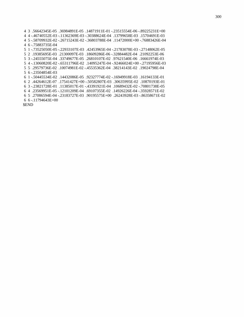
300

4 3 .56642345E-05 .36984891E-05 .14871911E-01 -.23515554E-06 -.89225231E+00

4 4 -.46740552E-03 -.11362369E-03 -.30388624E-04 .13799658E-03 .15704691E-03

4 5 -.58709932E-02 -.26715243E-02 -.36803788E-04 .11472000E+00 -.76883426E-04

4 6 -.75883735E-04

5 1 -.73525050E-05 -.22933107E-03 .42453965E-04 -.21783078E-03 -.27148062E-05

5 2 .19385695E-03 .21300097E-03 .18609286E-06 -.32884482E-04 .21092253E-06

5 3 -.24555075E-04 .33749677E-05 .26810107E-02 .97621540E-06 .16661974E-03

5 4 -.13060820E-02 -.65311796E-02 .14095247E-04 -.92466024E+00 -.27195956E-03

5 5 .29579736E-02 .10074981E-02 -.45535362E-04 .38214143E-02 .19024798E-04

5 6 -.23504854E-03

6 1 -.50445534E-02 .14432086E-05 .92327774E-02 -.16949918E-03 .16194133E-01

6 2 .44264612E-07 .17541427E+00 -.50582807E-03 .30635995E-02 .10870193E-01

6 3 -.23821728E-01 .11385017E-01 -.43391921E-04 .10689432E-02 -.70801738E-05

6 4 .23569951E-05 -.12101209E-04 .69107355E-02 .14926226E-04 -.35928571E-02

6 5 .27086594E-04 -.23183727E-03 .90195575E+00 .26243928E-03 -.86358671E-02

6 6 -.11794643E+00

$END

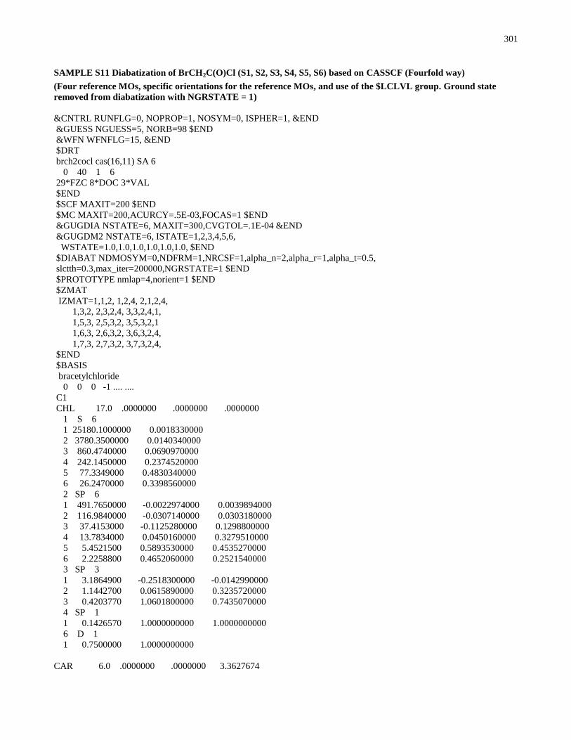
301

SAMPLE S11 Diabatization of BrCH2C(O)Cl (S1, S2, S3, S4, S5, S6) based on CASSCF (Fourfold way)

(Four reference MOs, specific orientations for the reference MOs, and use of the $LCLVL group. Ground state

removed from diabatization with NGRSTATE = 1)

&CNTRL RUNFLG=0, NOPROP=1, NOSYM=0, ISPHER=1, &END

&GUESS NGUESS=5, NORB=98 $END


$DRT

brch2cocl cas(16,11) SA 6

0 40 1 6

29*FZC 8*DOC 3*VAL

$END

$SCF MAXIT=200 $END

$MC MAXIT=200,ACURCY=.5E-03,FOCAS=1 $END

&GUGDIA NSTATE=6, MAXIT=300,CVGTOL=.1E-04 &END

&GUGDM2 NSTATE=6, ISTATE=1,2,3,4,5,6,

WSTATE=1.0,1.0,1.0,1.0,1.0,1.0, $END

$DIABAT NDMOSYM=0,NDFRM=1,NRCSF=1,alpha_n=2,alpha_r=1,alpha_t=0.5,

slctth=0.3,max_iter=200000,NGRSTATE=1 $END

$PROTOTYPE nmlap=4,norient=1 $END

$ZMAT

IZMAT=1,1,2, 1,2,4, 2,1,2,4,

1,3,2, 2,3,2,4, 3,3,2,4,1,

1,5,3, 2,5,3,2, 3,5,3,2,1

1,6,3, 2,6,3,2, 3,6,3,2,4,

1,7,3, 2,7,3,2, 3,7,3,2,4,

$END

$BASIS

bracetylchloride

0 0 0 -1 .... ....

C1

CHL 17.0 .0000000 .0000000 .0000000

1 S 6

1 25180.1000000 0.0018330000

2 3780.3500000 0.0140340000

3 860.4740000 0.0690970000

4 242.1450000 0.2374520000

5 77.3349000 0.4830340000

6 26.2470000 0.3398560000

2 SP 6

1 491.7650000 -0.0022974000 0.0039894000

2 116.9840000 -0.0307140000 0.0303180000

3 37.4153000 -0.1125280000 0.1298800000

4 13.7834000 0.0450160000 0.3279510000

5 5.4521500 0.5893530000 0.4535270000

6 2.2258800 0.4652060000 0.2521540000

3 SP 3

1 3.1864900 -0.2518300000 -0.0142990000

2 1.1442700 0.0615890000 0.3235720000

3 0.4203770 1.0601800000 0.7435070000

4 SP 1

1 0.1426570 1.0000000000 1.0000000000

6 D 1

1 0.7500000 1.0000000000

CAR 6.0 .0000000 .0000000 3.3627674

302

1 S 6

1 3047.5249000 0.0018347000

2 457.3695100 0.0140373000

3 103.9486900 0.0688426000

4 29.2101550 0.2321844000

5 9.2866630 0.4679413000

6 3.1639270 0.3623120000

2 SP 3

1 7.8682724 -0.1193324000 0.0689991000

2 1.8812885 -0.1608542000 0.3164240000

3 0.5442493 1.1434564000 0.7443083000

3 SP 1

1 0.1687144 1.0000000000 1.0000000000

4 D 1

1 0.8000000 1.0000000000

CAR 6.0 2.5502306 .0000000 4.5682559

1 S 6

1 3047.5249000 0.0018347000

2 457.3695100 0.0140373000

3 103.9486900 0.0688426000

4 29.2101550 0.2321844000

5 9.2866630 0.4679413000

6 3.1639270 0.3623120000

2 SP 3

1 7.8682724 -0.1193324000 0.0689991000

2 1.8812885 -0.1608542000 0.3164240000

3 0.5442493 1.1434564000 0.7443083000

3 SP 1

1 0.1687144 1.0000000000 1.0000000000

4 D 1

1 0.8000000 1.0000000000

OXY 8.0 -2.0016811 .0000000 4.9266521

1 S 6

1 5484.6717000 0.0018311000

2 825.2349500 0.0139501000

3 188.0469600 0.0684451000

4 52.9645000 0.2327143000

5 16.8975700 0.4701930000

6 5.7996353 0.3585209000

2 SP 3

1 15.5396160 -0.1107775000 0.0708743000

2 3.5999336 -0.1480263000 0.3397528000

3 1.0137618 1.1307670000 0.7271586000

3 SP 1

1 0.2700058 1.0000000000 1.0000000000

4 D 1

1 0.8000000 1.0000000000

BRO 35.0 5.2333603 .0000000 1.9223308

1 S 8

1 574300.0000000 0.0002204000

2 89070.0000000 0.0016871000

3 20210.0000000 0.0087457000

4 5736.0000000 0.0355970000

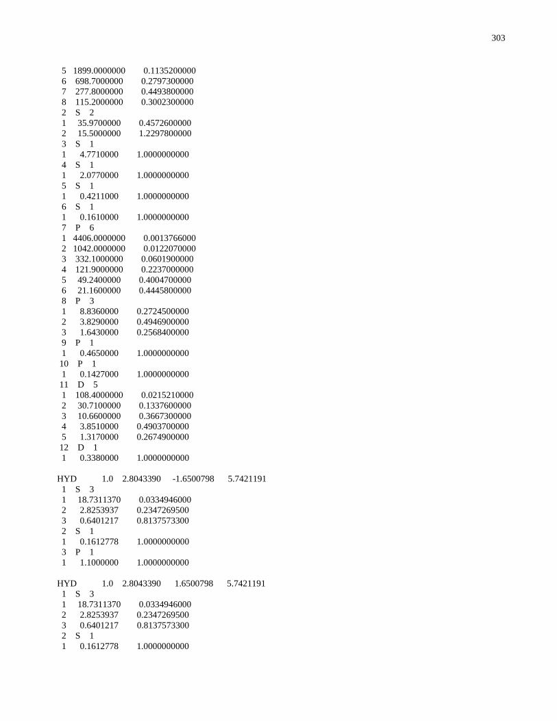
303

5 1899.0000000 0.1135200000

6 698.7000000 0.2797300000

7 277.8000000 0.4493800000

8 115.2000000 0.3002300000

2 S 2

1 35.9700000 0.4572600000

2 15.5000000 1.2297800000

3 S 1

1 4.7710000 1.0000000000

4 S 1

1 2.0770000 1.0000000000

5 S 1

1 0.4211000 1.0000000000

6 S 1

1 0.1610000 1.0000000000

7 P 6

1 4406.0000000 0.0013766000

2 1042.0000000 0.0122070000

3 332.1000000 0.0601900000

4 121.9000000 0.2237000000

5 49.2400000 0.4004700000

6 21.1600000 0.4445800000

8 P 3

1 8.8360000 0.2724500000

2 3.8290000 0.4946900000

3 1.6430000 0.2568400000

9 P 1

1 0.4650000 1.0000000000

10 P 1

1 0.1427000 1.0000000000

11 D 5

1 108.4000000 0.0215210000

2 30.7100000 0.1337600000

3 10.6600000 0.3667300000

4 3.8510000 0.4903700000

5 1.3170000 0.2674900000

12 D 1

1 0.3380000 1.0000000000

HYD 1.0 2.8043390 -1.6500798 5.7421191

1 S 3

1 18.7311370 0.0334946000

2 2.8253937 0.2347269500

3 0.6401217 0.8137573300

2 S 1

1 0.1612778 1.0000000000

3 P 1

1 1.1000000 1.0000000000

HYD 1.0 2.8043390 1.6500798 5.7421191

1 S 3

1 18.7311370 0.0334946000

2 2.8253937 0.2347269500

3 0.6401217 0.8137573300

2 S 1

1 0.1612778 1.0000000000

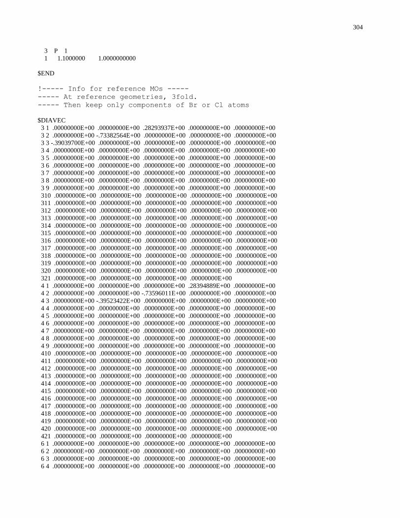
304

3 P 1

1 1.1000000 1.0000000000

$END

!----- Info for reference MOs -----

----- At reference geometries, 3fold.

----- Then keep only components of Br or Cl atoms

$DIAVEC

3 1 .00000000E+00 .00000000E+00 .28293937E+00 .00000000E+00 .00000000E+00

3 2 .00000000E+00 -.73382564E+00 .00000000E+00 .00000000E+00 .00000000E+00

3 3 -.39039700E+00 .00000000E+00 .00000000E+00 .00000000E+00 .00000000E+00

3 4 .00000000E+00 .00000000E+00 .00000000E+00 .00000000E+00 .00000000E+00

3 5 .00000000E+00 .00000000E+00 .00000000E+00 .00000000E+00 .00000000E+00

3 6 .00000000E+00 .00000000E+00 .00000000E+00 .00000000E+00 .00000000E+00

3 7 .00000000E+00 .00000000E+00 .00000000E+00 .00000000E+00 .00000000E+00

3 8 .00000000E+00 .00000000E+00 .00000000E+00 .00000000E+00 .00000000E+00

3 9 .00000000E+00 .00000000E+00 .00000000E+00 .00000000E+00 .00000000E+00

310 .00000000E+00 .00000000E+00 .00000000E+00 .00000000E+00 .00000000E+00

311 .00000000E+00 .00000000E+00 .00000000E+00 .00000000E+00 .00000000E+00

312 .00000000E+00 .00000000E+00 .00000000E+00 .00000000E+00 .00000000E+00

313 .00000000E+00 .00000000E+00 .00000000E+00 .00000000E+00 .00000000E+00

314 .00000000E+00 .00000000E+00 .00000000E+00 .00000000E+00 .00000000E+00

315 .00000000E+00 .00000000E+00 .00000000E+00 .00000000E+00 .00000000E+00

316 .00000000E+00 .00000000E+00 .00000000E+00 .00000000E+00 .00000000E+00

317 .00000000E+00 .00000000E+00 .00000000E+00 .00000000E+00 .00000000E+00

318 .00000000E+00 .00000000E+00 .00000000E+00 .00000000E+00 .00000000E+00

319 .00000000E+00 .00000000E+00 .00000000E+00 .00000000E+00 .00000000E+00

320 .00000000E+00 .00000000E+00 .00000000E+00 .00000000E+00 .00000000E+00

321 .00000000E+00 .00000000E+00 .00000000E+00 .00000000E+00

4 1 .00000000E+00 .00000000E+00 .00000000E+00 .28394889E+00 .00000000E+00

4 2 .00000000E+00 .00000000E+00 -.73596011E+00 .00000000E+00 .00000000E+00

4 3 .00000000E+00 -.39523422E+00 .00000000E+00 .00000000E+00 .00000000E+00

4 4 .00000000E+00 .00000000E+00 .00000000E+00 .00000000E+00 .00000000E+00

4 5 .00000000E+00 .00000000E+00 .00000000E+00 .00000000E+00 .00000000E+00

4 6 .00000000E+00 .00000000E+00 .00000000E+00 .00000000E+00 .00000000E+00

4 7 .00000000E+00 .00000000E+00 .00000000E+00 .00000000E+00 .00000000E+00

4 8 .00000000E+00 .00000000E+00 .00000000E+00 .00000000E+00 .00000000E+00

4 9 .00000000E+00 .00000000E+00 .00000000E+00 .00000000E+00 .00000000E+00

410 .00000000E+00 .00000000E+00 .00000000E+00 .00000000E+00 .00000000E+00

411 .00000000E+00 .00000000E+00 .00000000E+00 .00000000E+00 .00000000E+00

412 .00000000E+00 .00000000E+00 .00000000E+00 .00000000E+00 .00000000E+00

413 .00000000E+00 .00000000E+00 .00000000E+00 .00000000E+00 .00000000E+00

414 .00000000E+00 .00000000E+00 .00000000E+00 .00000000E+00 .00000000E+00

415 .00000000E+00 .00000000E+00 .00000000E+00 .00000000E+00 .00000000E+00

416 .00000000E+00 .00000000E+00 .00000000E+00 .00000000E+00 .00000000E+00

417 .00000000E+00 .00000000E+00 .00000000E+00 .00000000E+00 .00000000E+00

418 .00000000E+00 .00000000E+00 .00000000E+00 .00000000E+00 .00000000E+00

419 .00000000E+00 .00000000E+00 .00000000E+00 .00000000E+00 .00000000E+00

420 .00000000E+00 .00000000E+00 .00000000E+00 .00000000E+00 .00000000E+00

421 .00000000E+00 .00000000E+00 .00000000E+00 .00000000E+00

6 1 .00000000E+00 .00000000E+00 .00000000E+00 .00000000E+00 .00000000E+00

6 2 .00000000E+00 .00000000E+00 .00000000E+00 .00000000E+00 .00000000E+00

6 3 .00000000E+00 .00000000E+00 .00000000E+00 .00000000E+00 .00000000E+00

6 4 .00000000E+00 .00000000E+00 .00000000E+00 .00000000E+00 .00000000E+00

305

6 5 .00000000E+00 .00000000E+00 .00000000E+00 .00000000E+00 .00000000E+00

6 6 .00000000E+00 .00000000E+00 .00000000E+00 .00000000E+00 .00000000E+00

6 7 .00000000E+00 .00000000E+00 .00000000E+00 .00000000E+00 .00000000E+00

6 8 .00000000E+00 .00000000E+00 .00000000E+00 .00000000E+00 .00000000E+00

6 9 .00000000E+00 .00000000E+00 .00000000E+00 .00000000E+00 .00000000E+00

610 .00000000E+00 .00000000E+00 .00000000E+00 .00000000E+00 .00000000E+00

611 .00000000E+00 .00000000E+00 .00000000E+00 .00000000E+00 .00000000E+00

612 .00000000E+00 .00000000E+00 .00000000E+00 .00000000E+00 .00000000E+00

613 .00000000E+00 .00000000E+00 .00000000E+00 .00000000E+00 .00000000E+00

614 .00000000E+00 .00000000E+00 .00000000E+00 .00000000E+00 .00000000E+00

615 .00000000E+00 .00000000E+00 .00000000E+00 .33242447E+00 .00000000E+00

616 .00000000E+00 -.60498448E+00 .00000000E+00 .00000000E+00 -.52995857E+00

617 .00000000E+00 .00000000E+00 .00000000E+00 .00000000E+00 .00000000E+00

618 .00000000E+00 .00000000E+00 .00000000E+00 .00000000E+00 .00000000E+00

619 .00000000E+00 .00000000E+00 .00000000E+00 .00000000E+00 .00000000E+00

620 .00000000E+00 .00000000E+00 .00000000E+00 .00000000E+00 .00000000E+00

621 .00000000E+00 .00000000E+00 .00000000E+00 .00000000E+00

8 1 .00000000E+00 .00000000E+00 .00000000E+00 .00000000E+00 .00000000E+00

8 2 .00000000E+00 .00000000E+00 .00000000E+00 .00000000E+00 .00000000E+00

8 3 .00000000E+00 .00000000E+00 .00000000E+00 .00000000E+00 .00000000E+00

8 4 .00000000E+00 .00000000E+00 .00000000E+00 .00000000E+00 .00000000E+00

8 5 .00000000E+00 .00000000E+00 .00000000E+00 .00000000E+00 .00000000E+00

8 6 .00000000E+00 .00000000E+00 .00000000E+00 .00000000E+00 .00000000E+00

8 7 .00000000E+00 .00000000E+00 .00000000E+00 .00000000E+00 .00000000E+00

8 8 .00000000E+00 .00000000E+00 .00000000E+00 .00000000E+00 .00000000E+00

8 9 .00000000E+00 .00000000E+00 .00000000E+00 .00000000E+00 .00000000E+00

810 .00000000E+00 .00000000E+00 .00000000E+00 .00000000E+00 .00000000E+00

811 .00000000E+00 .00000000E+00 .00000000E+00 .00000000E+00 .00000000E+00

812 .00000000E+00 .00000000E+00 .00000000E+00 .00000000E+00 .00000000E+00

813 .00000000E+00 .00000000E+00 .00000000E+00 .00000000E+00 .00000000E+00

814 .00000000E+00 .00000000E+00 .00000000E+00 .00000000E+00 .00000000E+00

815 .00000000E+00 .00000000E+00 .00000000E+00 .00000000E+00 -.32510417E+00

816 .00000000E+00 .00000000E+00 .59077348E+00 .00000000E+00 .00000000E+00

817 .52436095E+00 .00000000E+00 .00000000E+00 .00000000E+00 .00000000E+00

818 .00000000E+00 .00000000E+00 .00000000E+00 .00000000E+00 .00000000E+00

819 .00000000E+00 .00000000E+00 .00000000E+00 .00000000E+00 .00000000E+00

820 .00000000E+00 .00000000E+00 .00000000E+00 .00000000E+00 .00000000E+00

821 .00000000E+00 .00000000E+00 .00000000E+00 .00000000E+00

$END

$LCLVL ! Definition of local frame for reference MOs !----- 1) Determine orientation of C-Br bond -----

----- 2) Calculate rotation matrix from specific to standard orientation.

----- All other atoms are always in their standard orientation

CHL 1.0000 .0000 0.0000

0.0000 1.0000 0.0000

0.0000 0.0000 1.0000

CAR 1.0000 .0000 0.0000

0.0000 1.0000 0.0000

0.0000 0.0000 1.0000

CAR 1.0000 .0000 0.0000

0.0000 1.0000 0.0000

0.0000 0.0000 1.0000

OXY 1.0000 .0000 0.0000

0.0000 1.0000 0.0000

306

0.0000 0.0000 1.0000

BRO 1.0000 .0000 0.0000

0.0000 1.0000 0.0000

0.0000 0.0000 1.0000

HYD 1.0000 .0000 0.0000

0.0000 1.0000 0.0000

0.0000 0.0000 1.0000

HYD 1.0000 .0000 0.0000

0.0000 1.0000 0.0000

0.0000 0.0000 1.0000

CHL 1.0000 .0000 0.0000

0.0000 1.0000 0.0000

0.0000 0.0000 1.0000

CAR 1.0000 .0000 0.0000

0.0000 1.0000 0.0000

0.0000 0.0000 1.0000

CAR 1.0000 .0000 0.0000

0.0000 1.0000 0.0000

0.0000 0.0000 1.0000

OXY 1.0000 .0000 0.0000

0.0000 1.0000 0.0000

0.0000 0.0000 1.0000

BRO 1.0000 .0000 0.0000

0.0000 1.0000 0.0000

0.0000 0.0000 1.0000

HYD 1.0000 .0000 0.0000

0.0000 1.0000 0.0000

0.0000 0.0000 1.0000

HYD 1.0000 .0000 0.0000

0.0000 1.0000 0.0000

0.0000 0.0000 1.0000

CHL 1.0000 .0000 0.0000

0.0000 1.0000 0.0000

0.0000 0.0000 1.0000

CAR 1.0000 .0000 0.0000

0.0000 1.0000 0.0000

0.0000 0.0000 1.0000

CAR 1.0000 .0000 0.0000

0.0000 1.0000 0.0000

0.0000 0.0000 1.0000

OXY 1.0000 .0000 0.0000

0.0000 1.0000 0.0000

0.0000 0.0000 1.0000

BRO 0.7034 0.0000 0.7108

0.0000 1.0000 0.0000

-0.7108 0.0000 0.7034

HYD 1.0000 .0000 0.0000

0.0000 1.0000 0.0000

0.0000 0.0000 1.0000

HYD 1.0000 .0000 0.0000

0.0000 1.0000 0.0000

0.0000 0.0000 1.0000

CHL 1.0000 .0000 0.0000

0.0000 1.0000 0.0000

0.0000 0.0000 1.0000

CAR 1.0000 .0000 0.0000

307

0.0000 1.0000 0.0000

0.0000 0.0000 1.0000

CAR 1.0000 .0000 0.0000

0.0000 1.0000 0.0000

0.0000 0.0000 1.0000

OXY 1.0000 .0000 0.0000

0.0000 1.0000 0.0000

0.0000 0.0000 1.0000

BRO 0.7034 0.0000 0.7108

0.0000 1.0000 0.0000

-0.7108 0.0000 0.7034

HYD 1.0000 .0000 0.0000

0.0000 1.0000 0.0000

0.0000 0.0000 1.0000

HYD 1.0000 .0000 0.0000

0.0000 1.0000 0.0000

0.0000 0.0000 1.0000

$END

...

$CSFDAT is the same as in sampleS8


…

308

LA FIN

Documents

HONDO - t1.chem.umn.edut1.chem.umn.edu/hondoplus/HONDOPLUS_Manual_v5.2... · Restriction of orbital rotation based on dominant CSFs ... MCSCF Geometry Optimization ... algorithm for