HOGgles: Visualizing Object Detection Features∗

Carl Vondrick, Aditya Khosla, Tomasz Malisiewicz, Antonio TorralbaMassachusetts Institute of Technology

{vondrick,khosla,tomasz,torralba}@csail.mit.edu

Abstract

We introduce algorithms to visualize feature spaces usedby object detectors. The tools in this paper allow a humanto put on ‘HOG goggles’ and perceive the visual world asa HOG based object detector sees it. We found that thesevisualizations allow us to analyze object detection systemsin new ways and gain new insight into the detector’s fail-ures. For example, when we visualize the features for highscoring false alarms, we discovered that, although they areclearly wrong in image space, they do look deceptively sim-ilar to true positives in feature space. This result suggeststhat many of these false alarms are caused by our choice offeature space, and indicates that creating a better learningalgorithm or building bigger datasets is unlikely to correctthese errors. By visualizing feature spaces, we can gain amore intuitive understanding of our detection systems.

1. IntroductionFigure 1 shows a high scoring detection from an ob-

ject detector with HOG features and a linear SVM classifier

trained on PASCAL. Despite our field’s incredible progress

in object recognition over the last decade, why do our de-

tectors still think that sea water looks like a car?

Unfortunately, computer vision researchers are often un-

able to explain the failures of object detection systems.

Some researchers blame the features, others the training set,

and even more the learning algorithm. Yet, if we wish to

build the next generation of object detectors, it seems cru-

cial to understand the failures of our current detectors.

In this paper, we introduce a tool to explain some of the

failures of object detection systems.1 We present algorithms

to visualize the feature spaces of object detectors. Since

features are too high dimensional for humans to directly in-

spect, our visualization algorithms work by inverting fea-

tures back to natural images. We found that these inversions

provide an intuitive and accurate visualization of the feature

spaces used by object detectors.

∗Previously: Inverting and Visualizing Features for Object Detection1Code is available online at http://mit.edu/vondrick/ihog

Figure 1: An image from PASCAL and a high scoring car

detection from DPM [8]. Why did the detector fail?

Figure 2: We show the crop for the false car detection from

Figure 1. On the right, we show our visualization of the

HOG features for the same patch. Our visualization reveals

that this false alarm actually looks like a car in HOG space.

Figure 2 shows the output from our visualization on the

features for the false car detection. This visualization re-

veals that, while there are clearly no cars in the original

image, there is a car hiding in the HOG descriptor. HOG

features see a slightly different visual world than what we

see, and by visualizing this space, we can gain a more intu-

itive understanding of our object detectors.

Figure 3 inverts more top detections on PASCAL for

a few categories. Can you guess which are false alarms?

Take a minute to study the figure since the next sentence

might ruin the surprise. Although every visualization looks

like a true positive, all of these detections are actually false

alarms. Consequently, even with a better learning algorithm

or more data, these false alarms will likely persist. In other

words, the features are to blame.

The principle contribution of this paper is the presenta-

tion of algorithms for visualizing features used in object de-

tection. To this end, we present four algorithms to invert

2013 IEEE International Conference on Computer Vision

1550-5499/13 $31.00 © 2013 IEEE

DOI 10.1109/ICCV.2013.8

1

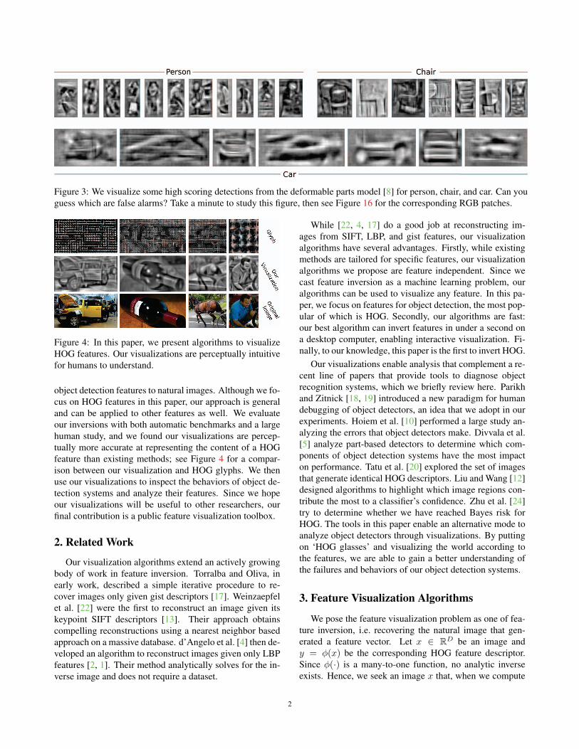
Figure 3: We visualize some high scoring detections from the deformable parts model [8] for person, chair, and car. Can you

guess which are false alarms? Take a minute to study this figure, then see Figure 16 for the corresponding RGB patches.

Figure 4: In this paper, we present algorithms to visualize

HOG features. Our visualizations are perceptually intuitive

for humans to understand.

object detection features to natural images. Although we fo-

cus on HOG features in this paper, our approach is general

and can be applied to other features as well. We evaluate

our inversions with both automatic benchmarks and a large

human study, and we found our visualizations are percep-

tually more accurate at representing the content of a HOG

feature than existing methods; see Figure 4 for a compar-

ison between our visualization and HOG glyphs. We then

use our visualizations to inspect the behaviors of object de-

tection systems and analyze their features. Since we hope

our visualizations will be useful to other researchers, our

final contribution is a public feature visualization toolbox.

2. Related Work

Our visualization algorithms extend an actively growing

body of work in feature inversion. Torralba and Oliva, in

early work, described a simple iterative procedure to re-

cover images only given gist descriptors [17]. Weinzaepfel

et al. [22] were the first to reconstruct an image given its

keypoint SIFT descriptors [13]. Their approach obtains

compelling reconstructions using a nearest neighbor based

approach on a massive database. d’Angelo et al. [4] then de-

veloped an algorithm to reconstruct images given only LBP

features [2, 1]. Their method analytically solves for the in-

verse image and does not require a dataset.

While [22, 4, 17] do a good job at reconstructing im-

ages from SIFT, LBP, and gist features, our visualization

algorithms have several advantages. Firstly, while existing

methods are tailored for specific features, our visualization

algorithms we propose are feature independent. Since we

cast feature inversion as a machine learning problem, our

algorithms can be used to visualize any feature. In this pa-

per, we focus on features for object detection, the most pop-

ular of which is HOG. Secondly, our algorithms are fast:

our best algorithm can invert features in under a second on

a desktop computer, enabling interactive visualization. Fi-

nally, to our knowledge, this paper is the first to invert HOG.

Our visualizations enable analysis that complement a re-

cent line of papers that provide tools to diagnose object

recognition systems, which we briefly review here. Parikh

and Zitnick [18, 19] introduced a new paradigm for human

debugging of object detectors, an idea that we adopt in our

experiments. Hoiem et al. [10] performed a large study an-

alyzing the errors that object detectors make. Divvala et al.

[5] analyze part-based detectors to determine which com-

ponents of object detection systems have the most impact

on performance. Tatu et al. [20] explored the set of images

that generate identical HOG descriptors. Liu and Wang [12]

designed algorithms to highlight which image regions con-

tribute the most to a classifier’s confidence. Zhu et al. [24]

try to determine whether we have reached Bayes risk for

HOG. The tools in this paper enable an alternative mode to

analyze object detectors through visualizations. By putting

on ‘HOG glasses’ and visualizing the world according to

the features, we are able to gain a better understanding of

the failures and behaviors of our object detection systems.

3. Feature Visualization Algorithms

We pose the feature visualization problem as one of fea-

ture inversion, i.e. recovering the natural image that gen-

erated a feature vector. Let x ∈ RD be an image and

y = φ(x) be the corresponding HOG feature descriptor.

Since φ(·) is a many-to-one function, no analytic inverse

exists. Hence, we seek an image x that, when we compute

2

Figure 5: We found that averaging the images of top detec-

tions from an exemplar LDA detector provide one method

to invert HOG features.

HOG on it, closely matches the original descriptor y:

φ−1(y) = argminx∈RD

||φ(x)− y||22 (1)

Optimizing Eqn.1 is challenging. Although Eqn.1 is not

convex, we tried gradient-descent strategies by numerically

evaluating the derivative in image space with Newton’s

method. Unfortunately, we observed poor results, likely be-

cause HOG is both highly sensitive to noise and Eqn.1 has

frequent local minima.

In the rest of this section, we present four algorithms for

inverting HOG features. Since, to our knowledge, no al-

gorithms to invert HOG have yet been developed, we first

describe three simple baselines for HOG inversion. We then

present our main inversion algorithm.

3.1. Baseline A: Exemplar LDA (ELDA)

Consider the top detections for the exemplar object de-

tector [9, 15] for a few images shown in Figure 5. Although

all top detections are false positives, notice that each detec-

tion captures some statistics about the query. Even though

the detections are wrong, if we squint, we can see parts of

the original object appear in each detection.

We use this simple observation to produce our first in-

version baseline. Suppose we wish to invert HOG feature y.

We first train an exemplar LDA detector [9] for this query,

w = Σ−1(y−μ). We score w against every sliding window

on a large database. The HOG inverse is then the average of

the top K detections in RGB space: φ−1A (y) = 1

K

∑Ki=1 zi

where zi is an image of a top detection.

This method, although simple, produces surprisingly ac-

curate reconstructions, even when the database does not

contain the category of the HOG template. However, it is

computationally expensive since it requires running an ob-

ject detector across a large database. We also point out that

a similar nearest neighbor method is used in brain research

to visualize what a person might be seeing [16].

3.2. Baseline B: Ridge Regression

We present a fast, parametric inversion baseline based

off ridge regression. Let X ∈ RD be a random variable

representing a gray scale image and Y ∈ Rd be a random

variable of its corresponding HOG point. We define these

random variables to be normally distributed on a D + d-

variate Gaussian P (X,Y ) ∼ N (μ,Σ) with parameters

μ = [ μX μY ] and Σ =[ΣXX ΣXY

ΣTXY ΣY Y

]. In order to invert a

HOG feature y, we calculate the most likely image from the

conditional Gaussian distribution P (X|Y = y):

φ−1B (y) = argmax

x∈RD

P (X = x|Y = y) (2)

It is well known that Gaussians have a closed form condi-

tional mode:

φ−1B (y) = ΣXY Σ

−1Y Y (y − μY ) + μX (3)

Under this inversion algorithm, any HOG point can be in-

verted by a single matrix multiplication, allowing for inver-

sion in under a second.

We estimate μ and Σ on a large database. In practice, Σis not positive definite; we add a small uniform prior (i.e.,

Σ = Σ +λI) so Σ can be inverted. Since we wish to in-

vert any HOG point, we assume that P (X,Y ) is stationary

[9], allowing us to efficiently learn the covariance across

massive datasets. We invert an arbitrary dimensional HOG

point by marginalizing out unused dimensions.

We found that ridge regression yields blurred inversions.

Intuitively, since HOG is invariant to shifts up to its bin size,

there are many images that map to the same HOG point.

Ridge regression is reporting the statistically most likely

image, which is the average over all shifts. This causes

ridge regression to only recover the low frequencies of the

original image.

3.3. Baseline C: Direct Optimization

We now provide a baseline that attempts to find im-

ages that, when we compute HOG on it, sufficiently match

the original descriptor. In order to do this efficiently, we

only consider images that span a natural image basis. Let

U ∈ RD×K be the natural image basis. We found using the

first K eigenvectors of ΣXX ∈ RD×D worked well for this

basis. Any image x ∈ RD can be encoded by coefficients

ρ ∈ RK in this basis: x = Uρ. We wish to minimize:

φ−1C (y) = Uρ∗

where ρ∗ = argminρ∈RK

||φ(Uρ)− y||22 (4)

Empirically we found success optimizing Eqn.4 using coor-

dinate descent on ρ with random restarts. We use an over-

complete basis corresponding to sparse Gabor-like filters

for U . We compute the eigenvectors of ΣXX across dif-

ferent scales and translate smaller eigenvectors to form U .

3.4. Algorithm D: Paired Dictionary Learning

In this section, we present our main inversion algorithm.

Let x ∈ RD be an image and y ∈ R

d be its HOG descriptor.

3

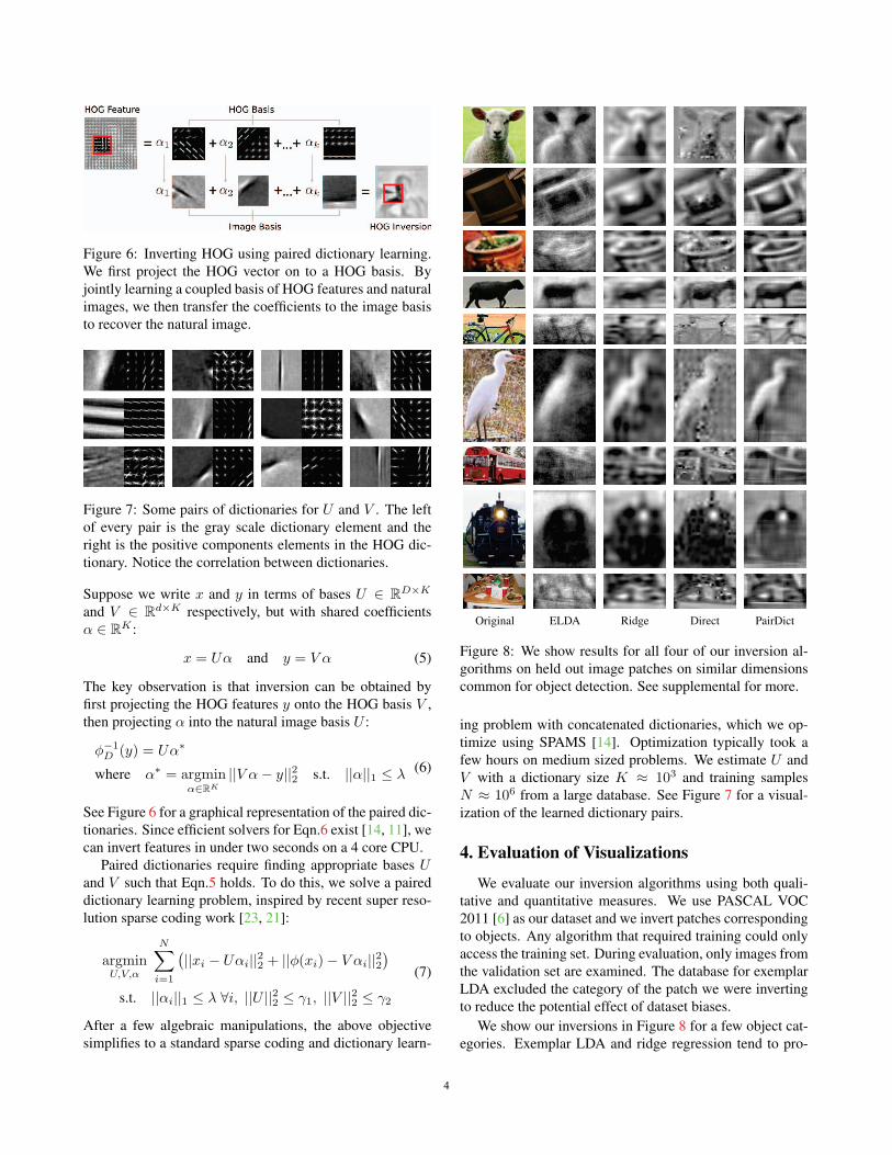
Figure 6: Inverting HOG using paired dictionary learning.

We first project the HOG vector on to a HOG basis. By

jointly learning a coupled basis of HOG features and natural

images, we then transfer the coefficients to the image basis

to recover the natural image.

Figure 7: Some pairs of dictionaries for U and V . The left

of every pair is the gray scale dictionary element and the

right is the positive components elements in the HOG dic-

tionary. Notice the correlation between dictionaries.

Suppose we write x and y in terms of bases U ∈ RD×K

and V ∈ Rd×K respectively, but with shared coefficients

α ∈ RK :

x = Uα and y = V α (5)

The key observation is that inversion can be obtained by

first projecting the HOG features y onto the HOG basis V ,

then projecting α into the natural image basis U :

φ−1D (y) = Uα∗

where α∗ = argminα∈RK

||V α− y||22 s.t. ||α||1 ≤ λ (6)

See Figure 6 for a graphical representation of the paired dic-

tionaries. Since efficient solvers for Eqn.6 exist [14, 11], we

can invert features in under two seconds on a 4 core CPU.

Paired dictionaries require finding appropriate bases Uand V such that Eqn.5 holds. To do this, we solve a paired

dictionary learning problem, inspired by recent super reso-

lution sparse coding work [23, 21]:

argminU,V,α

N∑i=1

(||xi − Uαi||22 + ||φ(xi)− V αi||22)

s.t. ||αi||1 ≤ λ ∀i, ||U ||22 ≤ γ1, ||V ||22 ≤ γ2

(7)

After a few algebraic manipulations, the above objective

simplifies to a standard sparse coding and dictionary learn-

Original ELDA Ridge Direct PairDict

Figure 8: We show results for all four of our inversion al-

gorithms on held out image patches on similar dimensions

common for object detection. See supplemental for more.

ing problem with concatenated dictionaries, which we op-

timize using SPAMS [14]. Optimization typically took a

few hours on medium sized problems. We estimate U and

V with a dictionary size K ≈ 103 and training samples

N ≈ 106 from a large database. See Figure 7 for a visual-

ization of the learned dictionary pairs.

4. Evaluation of Visualizations

We evaluate our inversion algorithms using both quali-

tative and quantitative measures. We use PASCAL VOC

2011 [6] as our dataset and we invert patches corresponding

to objects. Any algorithm that required training could only

access the training set. During evaluation, only images from

the validation set are examined. The database for exemplar

LDA excluded the category of the patch we were inverting

to reduce the potential effect of dataset biases.

We show our inversions in Figure 8 for a few object cat-

egories. Exemplar LDA and ridge regression tend to pro-

4

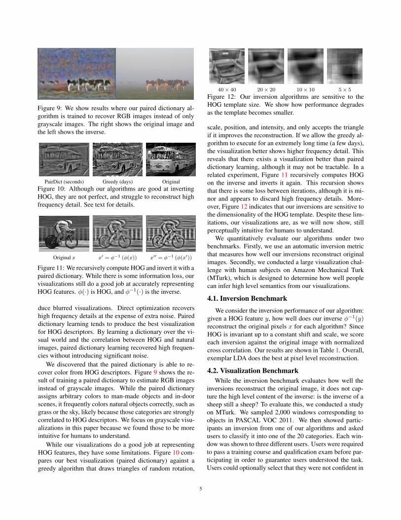
Figure 9: We show results where our paired dictionary al-

gorithm is trained to recover RGB images instead of only

grayscale images. The right shows the original image and

the left shows the inverse.

PairDict (seconds) Greedy (days) Original

Figure 10: Although our algorithms are good at inverting

HOG, they are not perfect, and struggle to reconstruct high

frequency detail. See text for details.

Original x x′ = φ−1 (φ(x)) x′′ = φ−1 (φ(x′))

Figure 11: We recursively compute HOG and invert it with a

paired dictionary. While there is some information loss, our

visualizations still do a good job at accurately representing

HOG features. φ(·) is HOG, and φ−1(·) is the inverse.

duce blurred visualizations. Direct optimization recovers

high frequency details at the expense of extra noise. Paired

dictionary learning tends to produce the best visualization

for HOG descriptors. By learning a dictionary over the vi-

sual world and the correlation between HOG and natural

images, paired dictionary learning recovered high frequen-

cies without introducing significant noise.

We discovered that the paired dictionary is able to re-

cover color from HOG descriptors. Figure 9 shows the re-

sult of training a paired dictionary to estimate RGB images

instead of grayscale images. While the paired dictionary

assigns arbitrary colors to man-made objects and in-door

scenes, it frequently colors natural objects correctly, such as

grass or the sky, likely because those categories are strongly

correlated to HOG descriptors. We focus on grayscale visu-

alizations in this paper because we found those to be more

intuitive for humans to understand.

While our visualizations do a good job at representing

HOG features, they have some limitations. Figure 10 com-

pares our best visualization (paired dictionary) against a

greedy algorithm that draws triangles of random rotation,

40× 40 20× 20 10× 10 5× 5

Figure 12: Our inversion algorithms are sensitive to the

HOG template size. We show how performance degrades

as the template becomes smaller.

scale, position, and intensity, and only accepts the triangle

if it improves the reconstruction. If we allow the greedy al-

gorithm to execute for an extremely long time (a few days),

the visualization better shows higher frequency detail. This

reveals that there exists a visualization better than paired

dictionary learning, although it may not be tractable. In a

related experiment, Figure 11 recursively computes HOG

on the inverse and inverts it again. This recursion shows

that there is some loss between iterations, although it is mi-

nor and appears to discard high frequency details. More-

over, Figure 12 indicates that our inversions are sensitive to

the dimensionality of the HOG template. Despite these lim-

itations, our visualizations are, as we will now show, still

perceptually intuitive for humans to understand.

We quantitatively evaluate our algorithms under two

benchmarks. Firstly, we use an automatic inversion metric

that measures how well our inversions reconstruct original

images. Secondly, we conducted a large visualization chal-

lenge with human subjects on Amazon Mechanical Turk

(MTurk), which is designed to determine how well people

can infer high level semantics from our visualizations.

4.1. Inversion Benchmark

We consider the inversion performance of our algorithm:

given a HOG feature y, how well does our inverse φ−1(y)reconstruct the original pixels x for each algorithm? Since

HOG is invariant up to a constant shift and scale, we score

each inversion against the original image with normalized

cross correlation. Our results are shown in Table 1. Overall,

exemplar LDA does the best at pixel level reconstruction.

4.2. Visualization BenchmarkWhile the inversion benchmark evaluates how well the

inversions reconstruct the original image, it does not cap-

ture the high level content of the inverse: is the inverse of a

sheep still a sheep? To evaluate this, we conducted a study

on MTurk. We sampled 2,000 windows corresponding to

objects in PASCAL VOC 2011. We then showed partic-

ipants an inversion from one of our algorithms and asked

users to classify it into one of the 20 categories. Each win-

dow was shown to three different users. Users were required

to pass a training course and qualification exam before par-

ticipating in order to guarantee users understood the task.

Users could optionally select that they were not confident in

5

Category ELDA Ridge Direct PairDict

bicycle 0.452 0.577 0.513 0.561

bottle 0.697 0.683 0.660 0.671

car 0.668 0.677 0.652 0.639

cat 0.749 0.712 0.687 0.705

chair 0.660 0.621 0.604 0.617

table 0.656 0.617 0.582 0.614

motorbike 0.573 0.617 0.549 0.592

person 0.696 0.667 0.646 0.646

Mean 0.671 0.656 0.620 0.637

Table 1: We evaluate the performance of our inversion al-

gorithm by comparing the inverse to the ground truth image

using the mean normalized cross correlation. Higher is bet-

ter; a score of 1 is perfect. See supplemental for full table.

Category ELDA Ridge Direct PairDict Glyph Expert

bicycle 0.327 0.127 0.362 0.307 0.405 0.438

bottle 0.269 0.282 0.283 0.446 0.312 0.222

car 0.397 0.457 0.617 0.585 0.359 0.389

cat 0.219 0.178 0.381 0.199 0.139 0.286

chair 0.099 0.239 0.223 0.386 0.119 0.167

table 0.152 0.064 0.162 0.237 0.071 0.125

motorbike 0.221 0.232 0.396 0.224 0.298 0.350

person 0.458 0.546 0.502 0.676 0.301 0.375

Mean 0.282 0.258 0.355 0.383 0.191 0.233

Table 2: We evaluate visualization performance across

twenty PASCAL VOC categories by asking MTurk work-

ers to classify our inversions. Numbers are percent classi-

fied correctly; higher is better. Chance is 0.05. Glyph refers

to the standard black-and-white HOG diagram popularized

by [3]. Paired dictionary learning provides the best visu-

alizations for humans. Expert refers to MIT PhD students

in computer vision performing the same visualization chal-

lenge with HOG glyphs. See supplemental for full table.

their answer. We also compared our algorithms against the

standard black-and-white HOG glyph popularized by [3].

Our results in Table 2 show that paired dictionary learn-

ing and direct optimization provide the best visualization

of HOG descriptors for humans. Ridge regression and ex-

emplar LDA performs better than the glyph, but they suf-

fer from blurred inversions. Human performance on the

HOG glyph is generally poor, and participants were even

the slowest at completing that study. Interestingly, the glyph

does the best job at visualizing bicycles, likely due to their

unique circular gradients. Our results overall suggest that

visualizing HOG with the glyph is misleading, and richer

visualizations from our paired dictionary are useful for in-

terpreting HOG vectors.

Our experiments suggest that humans can predict the

performance of object detectors by only looking at HOG

visualizations. Human accuracy on inversions and state-of-

the-art object detection AP scores from [7] are correlated

(a) Human Vision (b) HOG Vision

Figure 13: HOG inversion reveals the world that object de-

tectors see. The left shows a man standing in a dark room.

If we compute HOG on this image and invert it, the previ-

ously dark scene behind the man emerges. Notice the wall

structure, the lamp post, and the chair in the bottom right

hand corner.

with a Spearman’s rank correlation coefficient of 0.77.

We also asked computer vision PhD students at MIT to

classify HOG glyphs in order to compare MTurk workers

with experts in HOG. Our results are summarized in the

last column of Table 2. HOG experts performed slightly

better than non-experts on the glyph challenge, but experts

on glyphs did not beat non-experts on other visualizations.

This result suggests that our algorithms produce more intu-

itive visualizations even for object detection researchers.

5. Understanding Object DetectorsWe have so far presented four algorithms to visualize ob-

ject detection features. We evaluated the visualizations with

a large human study, and we found that paired dictionary

learning provides the most intuitive visualization of HOG

features. In this section, we will use this visualization to

inspect the behavior of object detection systems.

5.1. HOG Goggles

Our visualizations reveal that the world that features see

is slightly different from the world that the human eye per-

ceives. Figure 13a shows a normal photograph of a man

standing in a dark room, but Figure 13b shows how HOG

features see the same man. Since HOG is invariant to illu-

mination changes and amplifies gradients, the background

of the scene, normally invisible to the human eye, material-

izes in our visualization.

In order to understand how this clutter affects object de-

tection, we visualized the features of some of the top false

alarms from the Felzenszwalb et al. object detection sys-

tem [8] when applied to the PASCAL VOC 2007 test set.

6

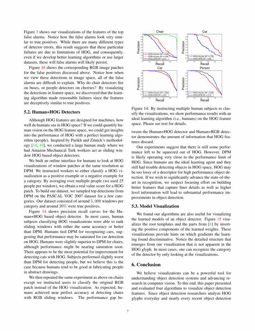
Figure 3 shows our visualizations of the features of the top

false alarms. Notice how the false alarms look very simi-

lar to true positives. While there are many different types

of detector errors, this result suggests that these particular

failures are due to limitations of HOG, and consequently,

even if we develop better learning algorithms or use larger

datasets, these will false alarms will likely persist.

Figure 16 shows the corresponding RGB image patches

for the false positives discussed above. Notice how when

we view these detections in image space, all of the false

alarms are difficult to explain. Why do chair detectors fire

on buses, or people detectors on cherries? By visualizing

the detections in feature space, we discovered that the learn-

ing algorithm made reasonable failures since the features

are deceptively similar to true positives.

5.2. Human+HOG Detectors

Although HOG features are designed for machines, how

well do humans see in HOG space? If we could quantify hu-

man vision on the HOG feature space, we could get insights

into the performance of HOG with a perfect learning algo-

rithm (people). Inspired by Parikh and Zitnick’s methodol-

ogy [18, 19], we conducted a large human study where we

had Amazon Mechanical Turk workers act as sliding win-

dow HOG based object detectors.

We built an online interface for humans to look at HOG

visualizations of window patches at the same resolution as

DPM. We instructed workers to either classify a HOG vi-

sualization as a positive example or a negative example for

a category. By averaging over multiple people (we used 25

people per window), we obtain a real value score for a HOG

patch. To build our dataset, we sampled top detections from

DPM on the PASCAL VOC 2007 dataset for a few cate-

gories. Our dataset consisted of around 5, 000 windows per

category and around 20% were true positives.

Figure 14 shows precision recall curves for the Hu-

man+HOG based object detector. In most cases, human

subjects classifying HOG visualizations were able to rank

sliding windows with either the same accuracy or better

than DPM. Humans tied DPM for recognizing cars, sug-

gesting that performance may be saturated for car detection

on HOG. Humans were slightly superior to DPM for chairs,

although performance might be nearing saturation soon.

There appears to be the most potential for improvement for

detecting cats with HOG. Subjects performed slightly worst

than DPM for detecting people, but we believe this is the

case because humans tend to be good at fabricating people

in abstract drawings.

We then repeated the same experiment as above on chairs

except we instructed users to classify the original RGB

patch instead of the HOG visualization. As expected, hu-

mans achieved near perfect accuracy at detecting chairs

with RGB sliding windows. The performance gap be-

0 0.2 0.4 0.6 0.8 10

0.1

0.2

0.3

0.4

0.5

0.6

0.7

0.8

0.9

1

Recall

Pre

cisi

on

Chair

HOG+Human AP = 0.63RGB+Human AP = 0.96HOG+DPM AP = 0.51

0 0.2 0.4 0.6 0.8 10

0.1

0.2

0.3

0.4

0.5

0.6

0.7

0.8

0.9

1

Recall

Pre

cisi

on

Cat

HOG+Human AP = 0.78HOG+DPM AP = 0.58

0 0.2 0.4 0.6 0.8 10

0.1

0.2

0.3

0.4

0.5

0.6

0.7

0.8

0.9

1

Recall

Pre

cisi

on

Car

HOG+Human AP = 0.83HOG+DPM AP = 0.87

0 0.2 0.4 0.6 0.8 10

0.1

0.2

0.3

0.4

0.5

0.6

0.7

0.8

0.9

1

Recall

Pre

cisi

on

Person

HOG+Human AP = 0.69HOG+DPM AP = 0.79

Figure 14: By instructing multiple human subjects to clas-

sify the visualizations, we show performance results with an

ideal learning algorithm (i.e., humans) on the HOG feature

space. Please see text for details.

tween the Human+HOG detector and Human+RGB detec-

tor demonstrates the amount of information that HOG fea-

tures discard.

Our experiments suggest that there is still some perfor-

mance left to be squeezed out of HOG. However, DPM

is likely operating very close to the performance limit of

HOG. Since humans are the ideal learning agent and they

still had trouble detecting objects in HOG space, HOG may

be too lossy of a descriptor for high performance object de-

tection. If we wish to significantly advance the state-of-the-

art in recognition, we suspect focusing effort on building

better features that capture finer details as well as higher

level information will lead to substantial performance im-

provements in object detection.

5.3. Model Visualization

We found our algorithms are also useful for visualizing

the learned models of an object detector. Figure 15 visu-

alizes the root templates and the parts from [8] by invert-

ing the positive components of the learned weights. These

visualizations provide hints on which gradients the learn-

ing found discriminative. Notice the detailed structure that

emerges from our visualization that is not apparent in the

HOG glyph. In most cases, one can recognize the category

of the detector by only looking at the visualizations.

6. ConclusionWe believe visualizations can be a powerful tool for

understanding object detection systems and advancing re-

search in computer vision. To this end, this paper presented

and evaluated four algorithms to visualize object detection

features. Since object detection researchers analyze HOG

glyphs everyday and nearly every recent object detection

7

Figure 15: We visualize a few deformable parts models trained with [8]. Notice the structure that emerges with our visual-

ization. First row: car, person, bottle, bicycle, motorbike, potted plant. Second row: train, bus, horse, television, chair. For

the right most visualizations, we also included the HOG glyph. Our visualizations tend to reveal more detail than the glyph.

Figure 16: We show the original RGB patches that correspond to the visualizations from Figure 3. We print the original

patches on a separate page to highlight how the inverses of false positives look like true positives. We recommend comparing

this figure side-by-side with Figure 3.

paper includes HOG visualizations, we hope more intuitive

visualizations will prove useful for the community.

Acknowledgments: We thank Hamed Pirsiavash, Joseph Lim, MIT

CSAIL Vision Group, and reviewers. Funding was provided by a NSF

GRFP to CV, a Facebook fellowship to AK, and a Google research award,

ONR MURI N000141010933 and NSF Career Award No. 0747120 to AT.

References[1] A. Alahi, R. Ortiz, and P. Vandergheynst. Freak: Fast retina keypoint.

In CVPR, 2012. 2

[2] M. Calonder, V. Lepetit, C. Strecha, and P. Fua. Brief: Binary robust

independent elementary features. ECCV, 2010. 2

[3] N. Dalal and B. Triggs. Histograms of oriented gradients for human

detection. In CVPR, 2005. 6

[4] E. d’Angelo, A. Alahi, and P. Vandergheynst. Beyond bits: Recon-

structing images from local binary descriptors. ICPR, 2012. 2

[5] S. Divvala, A. Efros, and M. Hebert. How important are deformable

parts in the deformable parts model? Technical Report, 2012. 2

[6] M. Everingham, L. Van Gool, C. K. I. Williams, J. Winn, and A. Zis-

serman. The pascal visual object classes challenge. IJCV, 2010. 4

[7] P. Felzenszwalb, R. Girshick, and D. McAllester. Cascade object

detection with deformable part models. In CVPR, 2010. 6

[8] P. Felzenszwalb, R. Girshick, D. McAllester, and D. Ramanan. Ob-

ject detection with discriminatively trained part-based models. PAMI,2010. 1, 2, 6, 7, 8

[9] B. Hariharan, J. Malik, and D. Ramanan. Discriminative decorrela-

tion for clustering and classification. ECCV, 2012. 3

[10] D. Hoiem, Y. Chodpathumwan, and Q. Dai. Diagnosing error in

object detectors. ECCV, 2012. 2

[11] H. Lee, A. Battle, R. Raina, and A. Ng. Efficient sparse coding algo-

rithms. NIPS, 2007. 4

[12] L. Liu and L. Wang. What has my classifier learned? visualizing the

classification rules of bag-of-feature model by support region detec-

tion. In CVPR, 2012. 2

[13] D. Lowe. Object recognition from local scale-invariant features. In

ICCV, 1999. 2

[14] J. Mairal, F. Bach, J. Ponce, and G. Sapiro. Online dictionary learn-

ing for sparse coding. In ICML, 2009. 4

[15] T. Malisiewicz, A. Gupta, and A. Efros. Ensemble of exemplar-svms

for object detection and beyond. In ICCV, 2011. 3

[16] S. Nishimoto, A. Vu, T. Naselaris, Y. Benjamini, B. Yu, and J. Gal-

lant. Reconstructing visual experiences from brain activity evoked

by natural movies. Current Biology, 2011. 3

[17] A. Oliva and A. Torralba. Modeling the shape of the scene: A holistic

representation of the spatial envelope. IJCV, 2001. 2

[18] D. Parikh and C. Zitnick. Human-debugging of machines. In NIPSWCSSWC, 2011. 2, 7

[19] D. Parikh and C. L. Zitnick. The role of features, algorithms and data

in visual recognition. In CVPR, 2010. 2, 7

[20] A. Tatu, F. Lauze, M. Nielsen, and B. Kimia. Exploring the repre-

sentation capabilities of hog descriptors. In ICCV WIT, 2011. 2

[21] S. Wang, L. Zhang, Y. Liang, and Q. Pan. Semi-coupled dictio-

nary learning with applications to image super-resolution and photo-

sketch synthesis. In CVPR, 2012. 4

[22] P. Weinzaepfel, H. Jegou, and P. Perez. Reconstructing an image

from its local descriptors. In CVPR, 2011. 2

[23] J. Yang, J. Wright, T. Huang, and Y. Ma. Image super-resolution via

sparse representation. Transactions on Image Processing, 2010. 4

[24] X. Zhu, C. Vondrick, D. Ramanan, and C. Fowlkes. Do we need

more training data or better models for object detection? BMVC,

2012. 2

8