High-resolution FEM-FCT schemes for

multidimensional conservation laws

D. Kuzmin∗, M. Moller and S. Turek

Institute of Applied Mathematics (LS III), University of Dortmund

Vogelpothsweg 87, D-44227, Dortmund, Germany

Abstract

The flux-corrected-transport paradigm is generalized to implicit finite elementschemes and nonlinear systems of hyperbolic conservation laws. In the scalar case, anonoscillatory low-order method of upwind type is derived by elimination of negativeoff-diagonal entries of the discrete transport operator. The difference between thediscretizations of high and low order is decomposed into a sum of skew-symmetricantidiffusive fluxes. An iterative flux limiter independent of the time step is proposedfor implicit schemes. The nonlinear antidiffusion is incorporated into the solutionin the framework of a defect correction scheme preconditioned by the monotonelow-order operator. In the case of a hyperbolic system, the global Jacobian matrixis assembled edge-by-edge without resorting to numerical integration. Its low-ordercounterpart is constructed by rendering all off-diagonal blocks positive definite oradding scalar artificial diffusion proportional to the spectral radius of the Roe ma-trix. The coupled equations are solved in a segregated manner within an outer de-fect correction loop equipped with a block-diagonal preconditioner. After a suitablesynchronization, the correction factors evaluated for an arbitrary set of indicatorvariables are applied to the antidiffusive fluxes which are inserted into the globaldefect vector. The performance of the new algorithm is illustrated by numericalexamples for scalar transport problems and the compressible Euler equations.

Key Words: convection-dominated flows; hyperbolic conservation laws;flux correction; finite elements; implicit time-stepping

1 Introduction

The flux-corrected-transport algorithm for convection-dominated flows was the first non-linear high-resolution scheme to switch between high- and low-order discretizations in anadaptive fashion depending on the local smoothness of the solution. Its foundations werelaid in the early 1970s by Boris and Book [3]. A genuinely multidimensional generaliza-tion of their celebrated SHASTA scheme was proposed by Zalesak [44] and successfullycarried over to finite elements by Lohner and his coworkers [27],[28]. The extension ofother high-resolution methods to unstructured meshes proved to be a rather challengingtask due to the one-dimensional nature of the underlying limiting techniques.

∗Correspondence to: kuzmin@math.uni-dortmund.de

1

Some finite element codes for compressible flow problems operate with numerical fluxesdesigned as in the finite difference context. To this end, a local one-dimensional stencilis reconstructed for each mesh edge by insertion of ‘dummy nodes’. The solution valuesat these nodes are obtained using a suitable interpolation/extrapolation technique, anda slope limiter is invoked to control the gradients. Unfortunately, the resulting FEMdiscretization may still produce nonphysical undershoots and overshoots in some cases.Moreover, the use of P1-elements is essential to the derivation of the underlying edge-based data structure as proposed by Peraire et al. [35]. An alternative flux decompositionprocedure, which is applicable to arbitrary finite elements, is introduced in our recentpublication devoted to a fully multidimensional flux limiter of TVD type [22].

In this paper, we present a generalized FEM-FCT formulation which is based ona representation of diffusive/antidiffusive terms as a sum of skew-symmetric internodalfluxes. A complete transition to a computationally efficient ‘edge-based’ data structure isfeasible but not mandatory [19],[22]. Hence, the algorithm to be presented can be readilyintegrated into an existing finite element code while preserving the conventional element-by-element matrix assembly and data access. It amounts to modifying the high-ordertransport operator so as to enforce the M-matrix property and render the discretizationlocal extremum diminishing. An in-depth description of the mathematical background isavailable in [17],[19],[20]. Our fully discrete approach distinguishes itself in that it dealswith finite element matrices regardless of the underlying mesh, approximation spaces andeven the number of spatial dimensions. Moreover, it can be used in conjunction withimplicit time-stepping schemes, unlike the classical FEM-FCT procedure.

We start with a summary of the new methodology for a scalar convection-diffusionequation and improve the algorithm in a number of ways. First of all, we observe thatZalesak’s limiter depends on the time step, so that the unconditional stability/positivityof our implicit FEM-FCT schemes cannot be duly utilized. To rectify this, we introducean iterative limiting strategy, whereby the rejected antidiffusion can be ‘recycled’ andbuilt into the numerical solution during the subsequent defect correction steps. Further-more, we clarify the origin of spurious ripples which may develop at the boundary andpropagate into the interior of the computational domain. It turned out that this alarmingphenomenon first mentioned in [17] is due to failure of the standard FCT algorithm todetermine correct upper and lower bounds for the solution values at the inlet and outlet.

The second part of this paper deals with a generalization of implicit FEM-FCT schemesto the Euler equations of gas dynamics. This is a continuation of the research reportedin our previous publications [19],[20]. The issues to be addressed include the assembly ofthe global Jacobian matrix, the iterative treatment of nonlinearities, the construction ofa nonoscillatory low-order scheme for systems of hyperbolic conservation laws, a propersynchronization of correction factors for decoupled variables and the implementation ofboundary conditions. We will show that many elements of the mathematical theoryand finite difference algorithms developed for the one-dimensional Euler equations canbe incorporated into the finite element framework. Due to the fact that the system athand is strongly nonlinear to begin with, the overhead cost incurred by the iterative fluxcorrection is not very significant. Encouraging results obtained for a number of standardtwo-dimensional test problems demonstrate the potential of the new method.

2

2 Galerkin FEM for scalar equations

Consider a generic time-dependent conservation law for a scalar quantity u

∂u

∂t+ ∇ · f = q in Ω, (1)

where q is a source term and f is a (nonlinear) flux function. Let us assume that it iscomposed from convective fluxes of the form fc = vu and diffusive fluxes of the formfd = −ǫ∇u. The weak form of the resulting convection-diffusion equation reads

∫

Ω

w

[

∂u

∂t+ ∇ · (vu − ǫ∇u) − q

]

dx = 0, ∀w. (2)

A common practice in finite element methods for conservation laws is to interpolateconvective fluxes and source terms in the same way as the numerical solution

u =∑

j

ujϕj, fc =∑

j

(vjuj) ϕj, q =∑

j

qjϕj, (3)

where ϕi denote the basis functions spanning the finite-dimensional subspace. This kindof approximation was called the group finite element formulation by Fletcher [7] whofound it to provide a very efficient treatment of nonlinear convective terms and even leadto a small gain of accuracy for the 2D Burgers equation discretized on a uniform grid.

The resulting Galerkin discretization of equation (1) reads

∑

j

[∫

Ω

ϕiϕj dx

]

(uj − qj) +∑

j

[∫

Ω

(ϕivj · ∇ϕj + ǫ∇ϕi · ∇ϕj) dx

]

uj = 0. (4)

It is implied that the diffusive flux vanishes at the boundary, so that the surface integralarising from the integration by parts can be omitted. Note that for most finite elements thesum of basis functions equals unity:

∑

i ϕi ≡ 1. Summing the semi-discretized equationsover i, one recovers the integral form of the conservation law, which ensures that the totalamount of u in Ω may only change due to boundary fluxes and internal sources or sinks.This shows that the Galerkin method enjoys the global conservation property.

The above system of ordinary differential equations for the nodal values of the approx-imate solution can be written compactly in matrix form

MC

du

dt= Ku + MC q, (5)

where MC = mij denotes the consistent mass matrix and K = kij stands for thediscrete transport operator. The matrix entries are given by

mij =

∫

Ω

ϕiϕj dx, kij = −vj · cij − ǫ sij, (6)

where cij and sij result from the discretization of differential operators corresponding tothe first- and second-order derivatives, respectively

cij =

∫

Ω

ϕi∇ϕj dx, sij =

∫

Ω

∇ϕi · ∇ϕj dx. (7)

3

Note that the coefficients mij, cij, sij remain unchanged as long as the mesh is fixed.Therefore, they need to be determined just once during the initialization phase. Thisenables us to update the matrix K in a very efficient way by computing its entries kij

from formula (6) without resorting to costly numerical integration. It is worth mentioningthat this shortcut is not essential for the subsequent considerations, so that the assemblyof the discrete transport operator can also be performed in the usual way.

3 Discrete upwinding

The FEM-FCT algorithm to be presented prevents the birth and growth of spuriousextrema by blending the oscillatory Galerkin discretization with a monotone low-ordermethod. The latter should be used in the vicinity of steep gradients, where nonphysicalundershoots and overshoots are likely to arise. In the realm of finite differences andfinite volumes, the upwind scheme is a perfect ‘wiggle-killer’. At the same time, it hasbeen largely unclear how to perform upwinding in the finite element framework. Mostof the upwind-like finite element methods encountered in the literature resort to a finitevolume discretization for the convective terms [2],[41]. An alternative derivation of theleast diffusive positivity-preserving scheme can be carried out by adding discrete diffusiondepending solely on the magnitude and position of negative matrix entries [16],[17]. Thisapproach will be elucidated below for the scalar transport equation and extended tohyperbolic systems of conservation laws in the second part of this paper.

Let us perform mass lumping and represent the ODE for a nodal value ui in the form

mi

dui

dt=

∑

j 6=i

kij(uj − ui) + riui + miqi, (8)

where mi =∑

j mij and ri =∑

j kij. The first term in the right-hand side of (8) isengendered by the incompressible part of the discrete transport operator, while riui is adiscrete counterpart of u∇ · v which vanishes for divergence-free velocity fields.

For the numerical solution to be nonoscillatory even close to shocks and discontinuities,all off-diagonal coefficients of K must be nonnegative: kij ≥ 0, j 6= i. This conditionis necessary to enforce the M-matrix property (see below) and make the discretizationlocal extremum diminishing (LED) for incompressible flows in the absence of source terms(ri = qi = 0). In this case, the semi-discrete scheme reduces to

dui

dt=

∑

j 6=i

cij(uj − ui), where cij =kij

mi

≥ 0. (9)

Such a discretization proves to be stable in the L∞-norm. Indeed, if ui is a maximum,then uj − ui ≤ 0, ∀j, so that dui

dt≤ 0. Hence, a maximum cannot increase, and similarly

a minimum cannot decrease. As a rule, the coefficient matrices are sparse, so that kij = 0unless i and j are adjacent nodes. Arguing as above, one can show that a local maximumcannot increase, and a local minimum cannot decrease. The LED criterion was introducedby Jameson [13],[14],[15] as a handy tool for the design of high-resolution schemes on un-structured meshes. It reduces to Harten’s TVD conditions [9],[10] in the one-dimensionalcase but remains valid in multidimensions and is easy to verify.

4

Any discrete transport operator K can be rendered local extremum diminishing byadding a tensor of artificial diffusion D = dij designed so as to eliminate its negativeoff-diagonal entries. The optimal diffusion coefficients are given by [17],[19]

dii = −∑

k 6=i

dik, dij = dji = max0,−kij,−kji. (10)

By construction, D is a generalized diffusion operator defined as a symmetric matrixhaving zero row and column sums [17]. Applying it to the vector u, we obtain

(Du)i =∑

j

dijuj =∑

j 6=i

dij(uj − ui) (11)

due to the zero row sum. Therefore, diffusive terms can be decomposed into a sum ofnumerical fluxes which reduce the difference between the nodal values

(Du)i =∑

j 6=i

fij, where fij = dij(uj − ui). (12)

Note that fji = −fij due to the symmetry of D. Hence, the insertion of artificial diffusiondoes not violate the discrete conservation principle. This kind of flux decomposition isfeasible for any generalized diffusion operator [17]. In the sequel, we will take advantageof this fact again and remove excessive diffusion in a mass-conserving fashion.

The elimination of negative matrix entries as proposed above yields the least diffusiveLED scheme obtainable from the original Galerkin discretization. For the pure convectionequation in one dimension, it is equivalent to the upwind difference method [17],[19]. Notethat physical diffusion (if any) built into the coefficients kij is automatically detected andthe amount of artificial diffusion is reduced accordingly. In diffusion-dominated cases, thediscrete transport operators K and L = K + D are identical, since the coefficients arenonnegative from the outset. Alternatively, this postprocessing technique can be appliedto the convective part of K without taking the physical diffusion into account.

Discrete upwinding should be performed edge-by-edge in accordance with the sparsitystructure of the finite element matrix. Let us start with the Galerkin operator L = K.For each pair of neighboring nodes i and j the required modification is as follows

lii = lii − dij, lij = lij + dij,

lji = lji + dij, ljj = ljj − dij.(13)

Let us emphasize that the LED constraint is imposed only on the incompressible partof the discrete transport operator K as it should be for physical reasons. The additionalterm riui + miqi in the right-hand side of (8) allows for an admissible growth and decayof local extrema due to compressibility and sources/sinks. In order to ensure that thepositivity of thermodynamic variables is reproduced by the numerical solution, this termmay need to be linearized as proposed by Patankar [34]. This procedure is described in ourprevious publications [19],[20] which should also be consulted for other algorithmic detailsand the underlying theory. For simplicity, we omit the source terms in what follows.

5

4 Defect correction

The equations at hand can be discretized in time by the standard θ-scheme. If implicittime-stepping (0 < θ ≤ 1) is employed, the nonlinearities inherent to the conservation lawand/or to the numerical method must be treated iteratively. Let us update the solutionin each outer iteration using the straightforward defect correction scheme

u(m+1) = u(m) + [A(u(m))]−1r(m), m = 0, 1, 2, . . . (14)

where r(m) denotes the residual vector for the m-th cycle and A is a suitably chosen‘preconditioner’ which should be easy to invert. The iteration process is terminated whenthe norm of the defect or that of the relative changes is small enough.

In a practical implementation, the ‘inversion’ of A is also performed by some iterativeprocedure. Hence, a certain number of inner iterations per cycle is required to solve thelinear subproblem for the solution increment which reads

A(u(m))∆u(m) = r(m). (15)

Afterwards, the correction ∆u(m) is applied to the last iterate

u(m+1) = u(m) + ∆u(m), u(0) = un. (16)

Note that the auxiliary problem (15) does not have to be solved very accurately at eachouter iteration. A moderate improvement of the residual (1-2 digits) is sufficient to obtaina good overall accuracy. The low-order evolution operator

A(u(m)) = ML − θ∆tL(u(m)), where ML = diagmi, (17)

constitutes an excellent preconditioner. It can be readily verified that A is an M-matrix,which makes it amenable to iterative solution. Furthermore, the diagonal dominance ofA can be enhanced by using an implicit underrelaxation strategy [6]. It will be notedthat defect correction preconditioned by the monotone upwind operator is widely used toenhance the robustness of CFD solvers even in the linear case. This is due to the fact thatan iterative method may fail to converge if applied directly to the ill-conditioned matrixoriginating from a high-order discretization of the bad-behaved convective terms.

The defect vector r(m) can be designed so as to obtain the standard Galerkin approx-imation, the diffusive low-order solution or a nonlinear combination thereof. The finiteelement discretizations of high and low order are related by the formula

r(m) = bn + f(un, u(m)) − A(u(m))u(m), (18)

where bn represents the right-hand side for the low-order scheme

bn = MLun + (1 − θ)∆tL(un)un, (19)

while the antidiffusion required to recover the high-order solution is given by

f(un, u(m)) = [(MC − ML) − (1 − θ)∆tD(un)]un

− [(MC − ML) + θ∆tD(u(m))]u(m). (20)

Here D = L−K denotes the artificial diffusion operator which transforms the oscillatoryhigh-order transport operator into the monotone low-order one as explained above.

6

By construction, D is a symmetric matrix with zero row and column sums, and so isthe operator MC −ML which is sometimes referred to as ‘mass diffusion’. Therefore, bothexpressions in the brackets represent discrete diffusion operators, so that the antidiffusiveterms can be decomposed into skew-symmetric internodal fluxes of the form

f(m)ij = [mij − (1 − θ)∆tdn

ij] (unj − un

i ) − [mij + θ∆td(m)ij ] (u

(m)j − u

(m)i ) = −f

(m)ji . (21)

These raw antidiffusive fluxes offset the error induced by mass lumping and discreteupwinding. In the fully explicit case (θ = 0) the convective terms must be stabilized bymeans of a streamline diffusion operator which also admits a flux decomposition [17],[19].In this paper we restrict ourselves to implicit finite element methods which do not requireany extra stabilization as far as the discretization is concerned. Linear Galerkin schemesof this type are of little use, as they are prone to nonphysical oscillations and lead tofinite element matrices with extremely unfavorable properties. At the same time, theyconstitute viable high-order methods for the flux-corrected-transport algorithm.

5 Iterative FEM-FCT formulation

The essence of flux correction consists in adding as much antidiffusion as possible withoutgenerating spurious wiggles. In particular, it is important to guarantee that quantitieslike densities, temperatures, concentrations etc. remain strictly nonnegative. It is obviousthat LED methods do satisfy this physically motivated constraint at the semi-discretelevel. However, the influence of the time discretization must also be taken into account.A fully discrete scheme is positivity-preserving if it can be represented in the form

Aun+1 = Bun, un ≥ 0, (22)

where A is an M-matrix and all entries of B are nonnegative [18],[19]. Building on thispositivity criterion, we will derive a nonlinear high-resolution scheme.

To begin with, let us analyze the defect correction method introduced above for themixture of high- and low-order discretizations. The substitution of (18) into (14) gives

A(u(m))u(m+1) = bn + f(un, u(m)). (23)

Recall that the low-order preconditioner A was designed to be an M-matrix. Hence, itsuffices to verify the positivity condition for the right-hand side. To this end, we introducean auxiliary quantity un as the solution to the explicit subproblem

MLun = MLun + (1 − θ)∆tL(un)un. (24)

In fact, un corresponds to an intermediate solution computed at the time instant tn+1−θ

by the explicit low-order method. Note that un = un in the fully implicit case θ = 1.Other time-stepping schemes preserve the positivity of un provided that [17],[19]

∆t ≤ 1

1 − θmin

i−mi/lii| lii < 0 . (25)

This readily computable upper bound follows from the positivity condition set forth aboveand can serve as a threshold value for an adaptive time step control.

7

According to (22), the positivity of un and un is inherited by u(m+1) if we drop thesecond term in the right-hand side of (23) and end up with bn = MLun. On the otherhand, the accuracy of the finite element discretization can be dramatically improved ifwe retain a certain portion of the antidiffusive fluxes in regions where the solution issufficiently smooth. The family of implicit FEM-FCT schemes proposed in [16],[17] isbased on the following representation of the right-hand side

b(m+1)i = bn

i +∑

j 6=i

α(m)ij f

(m)ij , α

(m)ij = αij(u

n, f(m)ij ). (26)

The involved correction factors α(m)ij depend on the auxiliary solution un and on the

interplay of raw antidiffusive fluxes. They are determined using the universal limitingstrategy presented in the next section. Roughly speaking, the flux correction step makessure that there exists a matrix B with no negative entries such that b(m+1) = Bun. Thisenables us to represent the discrete scheme in the desired form (22) with un in lieu of un.

Note that un is independent of the iteration number m and does not have to berecalculated in the course of defect correction. Unfortunately, there is a price to be paid forthis convenience. Namely, the numerical solution becomes increasingly diffusive at largetime steps. Equation (21) reveals that the spatial contribution to the raw antidiffusive fluxis proportional to the time step. At the same time, the amount of acceptable antidiffusiondepends solely on un, so that the flux must be drastically curtailed as its magnitudeincreases with the time step. This is a serious drawback, since the ability to operate withlarge time steps was the main reason for using an implicit scheme in the first place.

In order to alleviate the dependence of the final solution on the time step, we resort toan iterative FEM-FCT formulation, whereby only the rejected portion of the antidiffusiveflux needs to be dealt with. This prevents the flux limiter from returning to the worstcase scenario and makes the choice of correction factors at one particular iteration lesscritical. A somewhat similar technique was developed by Schar and Smolarkiewicz [37]in the finite difference context. However, their flux correction formalism is inherentlyexplicit, so that the advantages of using an iterative procedure are rather questionable forefficiency reasons. In addition, Schar and Smolarkiewicz determine the upper and lowerbounds using the old solution rather than the low-order one. This practice may turn outto be rather dangerous, especially for problems with sink terms [17],[19].

In our new approach, the accepted antidiffusion is incorporated into the intermediatesolution u(m) which is no longer fixed and must be updated along with the right-hand sideb(m) for the previous defect correction step

MLu(m) = b(m), b(0) = bn. (27)

Recall that ML is a diagonal matrix so that no linear system has to be solved and theoverhead cost associated with the computation of u(m) is negligible.

The limiting strategy remains unchanged except for the fact that the correction factorsare based on the local extrema of u(m) rather than un and applied to the difference betweenthe raw antidiffusive fluxes and the net effect of previous corrections

∆f(m)ij = f

(m)ij − g

(m)ij , α

(m)ij = αij(u

(m), ∆f(m)ij ). (28)

8

Subsequently, the limited flux difference is added to the sum of its predecessors

g(m+1)ij = g

(m)ij + α

(m)ij ∆f

(m)ij =

m∑

k=0

α(k)ij ∆f

(k)ij , g

(0)ij = 0 (29)

and inserted into the global load vector for the next iteration

b(m+1)i = b

(m)i +

∑

j 6=i

α(m)ij ∆f

(m)ij . (30)

In the special case α(m)ij ≡ 1, successive substitution yields

b(m+1)i = bn

i +∑

j 6=i

(g(m)ij + ∆f

(m)ij ) = bn

i +∑

j 6=i

f(m)ij . (31)

Therefore, our iterative FEM-FCT technique proves to be consistent in the sense that itreduces to the standard Galerkin discretization if no limiting is performed.

It is worth mentioning that (30) is of the same form as (26) and even equivalent to itfor m = 0. As before, the flux limiter ensures that b(m+1) = Bu(m) for some B ≥ 0, sothat the transformation u(m+1) = M−1

L Bu(m) as defined by the inverse diffusion problem(27) is positivity-preserving. Note that the classical FCT algorithm with un+1 = u(1) isrecovered in the fully explicit case (forward Euler time-stepping, lumped mass matrix).As the iteration process continues, more and more antidiffusion can be built into theintermediate solution. At the same time, the task of the flux limiter simplifies, becausethe remainder ∆f

(m)ij shrinks and a larger percentage of it can be accepted. This is in

contrast to the old approach, whereby the limiting procedure always starts from scratchwithout taking the outcome of previous flux correction steps into account.

In either case, the defect vector for the linear system (15) is redefined as

r(m) = b(m+1) − A(u(m))u(m), (32)

where b(m+1) consists of the low-order part bn and nonlinear antidiffusion. It remains todescribe the algorithm for the computation of correction factors and explain how it works.

6 Limiting strategy

The flux limiter is a key element of the FEM-FCT paradigm. As already pointed outabove, it is supposed to adjust the correction factors αij = αji so as to guarantee that

bi = miui +∑

j 6=i

αijfij ≥ 0 if u ≥ 0. (33)

Varying αij between zero and unity, one obtains the diffusive low-order solution, theoscillatory high-order solution or something in-between. If ui is a local extremum, thenthe antidiffusive fluxes trying to enhance it must be canceled completely by setting αij = 0.Otherwise, the following representation is feasible [16],[19]

bi = (mi − ci)ui + ciuk, where ci =

∑

j 6=i αijfij

uk − ui

(34)

and k is the number of a neighboring node at which a local extremum is attained.

9

A sufficient condition for the positivity constraint to be satisfied is given by the doubleinequality mi ≥ ci ≥ 0. Let umax

i and umini denote the maximum and minimum solution

values at the stencil Si which consists of node i and its nearest neighbors

umax

min

i =maxmin

uj, j ∈ Si. (35)

To make sure that ci ≥ 0, we adopt uk = umaxi if the net antidiffusive flux

∑

j 6=i αijfij

is positive and uk = umini otherwise. The remaining condition mi ≥ ci must be enforced

by tuning the correction factors. This can be accomplished by invoking Zalesak’s FCTlimiter which was originally derived using heuristic arguments and applicable only in theframework of an explicit time discretization.

Antidiffusive fluxes directed down the gradient of u tend to flatten solution profilesand should be canceled completely at the outset of the flux correction process

fij := 0, if fij(ui − uj) ≤ 0. (36)

In other words, an antidiffusive flux should not be allowed to act as a diffusive one.This optional prelimiting step can be traced back to the original SHASTA scheme [3].Zalesak mentioned it as well but argued that the resulting improvement is marginal andcosmetic in nature [44]. However, without this amendment his multidimensional limiteris positivity- but not monotonicity-preserving, so that the numerical solution may exhibitvarious artifacts in the vicinity of shocks and discontinuities [4],[17],[19].

Following Zalesak [44] and Lohner et al. [27], we introduce the auxiliary quantities

P±i =

1

mi

∑

j 6=i

max

min0, fij, Q±

i = umax

min

i − ui, (37)

which represent the sum of all positive/negative antidiffusive fluxes into node i and thedistance to the local extremum, respectively. In the worst case, all contributions are ofthe same sign, so that the flux fij should be multiplied by

R±i =

min1, Q±i /P±

i , if P±i 6= 0,

1, if P±i = 0.

(38)

Recall that a positive flux fij into node i is always balanced by a negative flux fji = −fij

into node j and vice versa. Hence, the limiter must inspect the sign of the flux and takethe minimum of the nodal correction factors

αij =

minR+i , R−

j , if fij ≥ 0,minR+

j , R−i , if fij < 0.

(39)

Note that Q±i = 0 implies R±

i = 0 and αij = 0. Hence, any enhancement of localextrema is prohibited by the limiter. Furthermore, the following estimate holds [17],[19]

miQ−i ≤ miR

−i P−

i ≤∑

j 6=i

αijfij ≤ miR+i P+

i ≤ miQ+i . (40)

This proves that the corrected antidiffusive fluxes satisfy the constraint mi ≥ ci.

10

7 Boundary treatment

It was reported in [17] that an FCT algorithm based on Zalesak’s limiter may malfunctionfor smooth solutions having a nonvanishing gradient at the boundary. In this case, smallripples may pop up at the outlet and propagate into the interior of the domain as illus-trated in Figure 1 (left) for the one-dimensional convection equation with v = 1, u0 = x.Similar problems occur at the inlet but their detrimental effect is alleviated by the Dirich-let boundary condition. Some preliminary speculations regarding the origin of spuriousripples can be found in [17]. Recently, an explanation of this phenomenon was given byMoller [32] who observed that formula (35) yields a poor estimate of upper/lower boundsat inflow and outflow boundaries. Namely, ui can be misinterpreted as a local extremumbecause it is only compared to nodal values of the solution within the domain. As long asno information regarding the solution behavior beyond the open boundary is available, it

is impossible to tell whether or not umax

min

i would be an extremum for the extended domain.As a rule of thumb, antidiffusive fluxes should neither create new minima/maxima, nor

accentuate already existing ones [44]. Ironically, this fundamental law of flux correctionturns out to be the cause of troubles at the boundary. The faulty flux limiter erroneouslyanticipates the enhancement of a local extremum and switches to the diffusive low-ordersolution, which entails a redistribution of mass due to the discrete conservation principle.Changing the solution value at one node is accompanied by an adjustment of those atthe neighboring nodes so that the total mass remains unchanged. To illustrate this effect,the so-called lever model was introduced in [32]. Let the piecewise-linear solution berepresented by levers of variable length hinged at their midpoints, which correspond tothe element mean values, and connected continuously with one another. Pulling downthe rightmost lever results in a shearing force which affects the slopes of all componentsas shown in Figure 1 (right). Furthermore, the implications of the optional prelimitingstep (36) can be explained in a similar way. Roughly speaking, diffusive fluxes rotate thelevers in the wrong direction, which results in the formation of kinks and flat plateausamidst a steep front. For further details, the interested reader is referred to [32].

Formation of ripples at the outlet

0.9 0.91 0.92 0.93 0.94 0.95 0.96 0.97 0.98 0.99 10.9

0.91

0.92

0.93

0.94

0.95

0.96

0.97

0.98

0.99

1

Lever model

Figure 1. Pathological behavior of Zalesak’s limiter.

11

To cure the pathological behavior of Zalesak’s limiter, we reset the nodal correctionfactors which are based on questionable upper/lower bounds

R±i := 1 ∀i ∈ Nb, (41)

where Nb denotes the set of nodes belonging to the inflow and outflow boundaries. Atthe inlet, it is reasonable to do so anyway because the essential boundary conditionoverrides the contribution of incoming antidiffusive fluxes. At the outlet, the off-diagonalcoefficients of the high-order transport operator are typically nonnegative [17],[22] so thismodification does not pose any hazard to positivity either. In addition, any undershoots orovershoots generated there would be immediately convected away. The newly introducedpostlimiting step should follow (38) and precede (39) in a practical implementation. Thissimple remedy produces the desired effect at virtually no additional cost.

8 Summary of the FEM-FCT algorithm

The revised Zalesak’s limiter completes our iterative FEM-FCT formulation which isapplicable to nonlinear conservation laws, multidimensional problems, unstructured finiteelement meshes and implicit time-stepping schemes. It can be implemented as a black-boxpostprocessing routine which operates with discrete operators regardless of their origin.The modifications are introduced in a sweep over numerical edges which correspond topairs of basis functions with overlapping supports. The list of edges is determined bythe sparsity pattern of the finite element matrix. Specifically, each edge ~ij is associatedwith a nonzero off-diagonal coefficient aij in the upper/lower triangular part. The mainalgorithmic steps to be performed in the scalar case can be summarized as follows:

In the matrix assembly routine:

1. Retrieve/compute the entries kij and kji of the high-order transport operator.

2. Determine the corresponding artificial diffusion coefficient dij from equation (10).

3. Substitute the diffusive flux (12) into the right-hand side bn (at the first iteration).

4. Update the four entries of the upwind-biased preconditioner A as required by (13).

5. Compute the antidiffusive flux (21) or (28) to be limited and inserted into b(m+1).

In the flux correction module:

6. Initialize/update u by solving the explicit subproblem (24) or (27).

7. Invoke Zalesak’s limiter with pre- and postlimiting to compute αij from (39).

8. Insert the limited antidiffusive fluxes into expressions (26) or (29),(30).

In the defect correction loop:

9. Solve the linear system (15) with the defect vector r(m) given by (32).

10. Update the solution according to (16) and proceed to the next iteration.

In what follows, we generalize the above algorithm to systems of hyperbolic conservationlaws and elucidate its implementation for the Euler equations of gas dynamics.

12

9 Euler equations

Compressible flows at high velocities are governed by the Euler equations which representa system of conservation laws for the mass, momentum and energy of an inviscid fluid

∂ρ

∂t+ ∇ · (ρv) = 0, (42)

∂(ρv)

∂t+ ∇ · (ρv ⊗ v) + ∇p = 0, (43)

∂(ρE)

∂t+ ∇ · (ρhv) = 0, (44)

where ρ, v, p, E and h = E + p/ρ stand for the density, velocity, pressure, total energyper unit mass and stagnation enthalpy, respectively. This system is complemented by anequation of state which relates the energy, pressure and density, for instance

p = (γ − 1)ρ

(

E − |v|22

)

. (45)

Here γ denotes the ratio of specific heats for a polytropic gas (γ = 1.4 for air).Introducing the vector of conservative variables U and the triple of fluxes for each

coordinate direction F = (F 1, F 2, F 3) defined as follows

U =

ρρv1

ρv2

ρv3

ρE

, F 1 =

ρv1

ρv21 + p

ρv1v2

ρv1v3

ρhv1

, F 2 =

ρv2

ρv1v2

ρv22 + p

ρv2v3

ρhv2

, F 3 =

ρv3

ρv1v3

ρv2v3

ρv23 + p

ρhv3

(46)

we can represent the Euler equations in the standard divergence form

∂U

∂t+ ∇ · F = 0, where ∇ · F =

3∑

d=1

∂F d

∂xd

. (47)

Furthermore, the chain rule yields a quasi-linear formulation, in which the spatial deriva-tives are applied to the conservative variables rather than fluxes. The resulting systemcan be written in terms of the Jacobian matrices A = (A1, A2, A3) such that [12]

∂U

∂t+ A · ∇U = 0, where A · ∇U =

3∑

d=1

Ad ∂U

∂xd

. (48)

It is worth mentioning that the fluxes are homogeneous functions of the conservativevariables, so that the relationship between the components of F and A is given by

F d = AdU, Ad =∂F d

∂U, d = 1, 2, 3. (49)

Due to the hyperbolicity of the Euler equations, any linear combination of the threeJacobians is diagonalizable with real eigenvalues. This is a very useful property whichwill lead us to a natural generalization of the discrete upwinding technique.

13

10 Galerkin matrix assembly

Implicit finite element methods are rarely used for numerical simulation of compressibleflows. Therefore, the issue of efficient matrix assembly has received little attention in theliterature. In this section, we present an edge-based assembly technique for the standardGalerkin discretization of the Euler equations. Let us start with the divergence form (47)and interpolate the fluxes using the group finite element formulation which yields

∑

j

[∫

Ω

ϕiϕj dx

]

dUj

dt+

∑

j

[∫

Ω

ϕi∇ϕj dx

]

· Fj = 0. (50)

In order to obtain a (non-)linear system of the form AU = B after an implicit timediscretization, we should represent the semi-discrete problem as follows

MC

dU

dt= KU, (51)

where MC is the block-diagonal mass matrix for the coupled system and K is a discretecounterpart of the operator −A · ∇ for the quasi-linear formulation (48).

Recall that the basis functions sum to unity, so that the sum of their derivativesvanishes. Hence, the coefficients cij defined in (7) satisfy cii = −∑

j 6=i cij and it followsfrom (50) that the right-hand side of the five coupled equations for node i is given by

(KU)i = −∑

j

cij · Fj = −∑

j 6=i

cij · (Fj − Fi). (52)

Furthermore, it was shown in Roe’s pioneering work on approximate Riemann solvers forhyperbolic conservation laws [36] that Fj −Fi = Aij(Uj −Ui), where Aij = (A1

ij, A2ij, A

3ij)

corresponds to the continuous Jacobian A evaluated at the intermediate state

ρij =√

ρiρj, vij =

√ρivi +

√ρjvj√

ρi +√

ρj

, hij =

√ρihi +

√ρjhj√

ρi +√

ρj

. (53)

The density-averaged quantities ρij, vij and hij are called the Roe mean values.In light of the above, equation (52) admits the following representation

(KU)i = −∑

j 6=i

cij · Aij(Uj − Ui), where cij · Aij =3

∑

d=1

cdijA

dij. (54)

The dot product can be interpreted as a ‘projection’ of the triple Aij onto the numerical

edge ~ij. For our purposes, it is expedient to introduce the splitting cij ·Aij = −(aij +bij),where the two components of the cumulative Roe matrix are defined by [20]

aij = aij · Aij, aij = −cij − cji

2, (55)

bij = bij · Aij, bij = −cij + cji

2. (56)

14

A similar decomposition can be performed for the contribution of node i to (KU)j

cji · (Fj − Fi) = cji · Aij(Uj − Ui), where cji · Aij = aij − bij. (57)

Furthermore, integration by parts reveals that the coefficients cij and cji are related by

cij + cji =

∫

Γ

nϕiϕj ds, (58)

where n denotes the outward unit normal to the boundary. Thus, we have

aij = −cij +1

2

∫

Γ

nϕiϕj ds, bij = −1

2

∫

Γ

nϕiϕj ds. (59)

For typical finite elements (linear and multilinear) the surface integral is nonzero onlyif both nodes belong to the boundary. Hence, aij = −cij in the interior of the domain,while bij = 0 and its contribution bij to the local Jacobian vanishes. This means thatjust one cumulative Roe matrix, namely aij, needs to be evaluated for each interior edge.At the boundary, one obtains bij = −n tij/2, where tij =

∫

Γϕiϕj ds corresponds to an

off-diagonal entry of the mass matrix for the surface triangulation. The Roe matrices forboundary edges consist of a skew-symmetric part aij and a symmetric part bij.

According to (54)–(57), the contribution of the edge ~ij to the term KU reads

(aij + bij)(Uj − Ui) −→ (KU) i (60)

(aij − bij)(Uj − Ui) −→ (KU)j (61)

This representation leads to a very efficient edge-based algorithm for matrix assembly.Now as before, there is no need for numerical integration as long as the coefficients cij

are initialized and stored. The graph representing the connectivity of the global matrixdepends solely on the underlying mesh and on the type of finite element approximation.For systems of equations, the array of edges remains the same as in the scalar case.However, there are interactions not only between basis functions for different nodes butalso between basis functions for different variables. Hence, each coefficient of the discreteoperator turns into a matrix of size equal to the squared number of variables.

It can be readily inferred from (60)–(61) that the four 5× 5 blocks contributed by thenumerical edge ~ij to the global Jacobian matrix K ∈ R

5N×5N are given by

kii = −aij − bij, kij = aij + bij,

kji = −aij + bij, kjj = aij − bij.(62)

These local Jacobians are evaluated edge-by-edge and their entries kklij (k, l = 1, . . . , 5)

are scattered to the corresponding positions in the 25 blocks Kkl ∈ RN×N . The assembly

process is illustrated in Figure 2. In practice, it is not necessary to assemble and storethe gigantic global matrix completely. Due to the nonlinearity of the Euler equations, theuse of an iterative solution technique is indispensable. If we employ the defect correctionmethod with a block-diagonal preconditioner (see below) then just the five blocks Kkk

will need to be generated explicitly. The remaining part of the matrix will be representedby the edge contributions (60)–(61) to be inserted directly into the defect vector.

15

11 Artificial viscosity

To a large extent, the ability of a FEM-FCT algorithm to withstand the formation ofwiggles depends on the quality of the underlying low-order method. In order to get rid ofoscillations, we perform mass lumping and replace the high-order system (51) by

ML

dU

dt= LU, (63)

where ML denotes the lumped mass matrix and L is the low-order Jacobian operator.Recall that we derived its scalar counterpart by elimination of negative off-diagonal entriesfrom the Galerkin operator. Now this discrete upwinding technique needs to be extendedto hyperbolic systems. In this case, the edge contributions to the global finite elementmatrix are no longer scalar quantities but matrices themselves. As a natural generalizationof the LED criterion, we require that all off-diagonal matrix blocks be positive definite.

To achieve the desired effect, we add tensorial artificial viscosity dij ∈ R5×5 to the

Roe matrices in (62). This straightforward transformation leads to

lii = −aij − dij, lij = aij + dij,

lji = −aij + dij, ljj = aij − dij,(64)

which corresponds to (13) in the scalar case. The modified edge contributions are builtinto the blocks of L as explained above. In essence, dij supersedes the symmetric partbij of the cumulative Roe matrix which belongs into the raw antidiffusive flux

fij = −(

mij

d

dt+ dij − bij

)

(Uj − Ui), fji = −fij. (65)

The block mij = mijI, where I denotes the 5×5 identity matrix, is responsible for the errorinduced by mass lumping. After the time discretization, one obtains an expression similarto (21). It remains to design dij so as to satisfy the generalized positivity constraint.

th rowi

th rowj

th columnith columnj

jikl

jjkl

ijkl

iikl

KK

K K

i j

i

j

l

k

Figure 2. Edge-based matrix assembly for the Euler equations.

16

As already mentioned, the system of Euler equations is hyperbolic, so that any linearcombination of the three Jacobian matrices is diagonalizable with real eigenvalues. Thus,there exists a diagonal matrix Λ(aij) and a regular matrix R(aij) of right eigenvectorssuch that the cumulative Roe matrix aij admits the following factorization

aij = R(aij)Λ(aij)R(aij)−1, (66)

where diagonal entries of the matrix

Λ(aij) = |aij|diag vij − cij, vij, vij, vij, vij + cij (67)

are proportional to the eigenvalues of aij. The scaling factor |aij| stands for the Euclideannorm of the coefficient vector aij, while the auxiliary quantities

vij =aij · vij

|aij|, cij =

√

(γ − 1)

(

hij −|vij|2

2

)

(68)

represent the ‘projection’ of the density-averaged velocity vij onto the numerical edge ~ijand the local speed of sound for this edge, respectively.

Making use of the characteristic decomposition (66), we can eliminate the negativeeigenvalues of aij and define the tensor dij as follows

dij = |aij| = R(aij) |Λ(aij)|R(aij)−1, (69)

where the matrix |Λ(aij)| contains the absolute values of the eigenvalues

|Λ(aij)| = |aij|diag |vij − cij|, |vij|, |vij|, |vij|, |vij + cij| . (70)

This kind of artificial viscosity is frequently employed to construct upwind-biased finitedifference schemes for hyperbolic systems [12],[24],[31]. The approach presented in thispaper enables us to incorporate it into a finite element discretization and obtain an analogof Roe’s approximate Riemann solver based on flux difference splitting.

As an alternative, discrete upwinding for systems of equations can be performed inthe framework of the conservative flux decomposition outlined in [19],[20],[22]

(KU)i = −∑

j 6=i

gij, where gij = cij · Fi − cji · Fj. (71)

Note that the so-defined Galerkin fluxes are skew-symmetric: gji = −gij. On a uniform1D mesh, cij = ±1/2 for linear finite elements, so that gij = ±(Fi + Fj)/2. This isdue to the well-known fact that the Galerkin method results in a central difference typeapproximation. The replacement of gij by the consistent numerical flux

g∗ij = gij −

1

2dij(Uj − Ui) (72)

yields the same nonoscillatory low-order scheme as the one derived above [19],[20].

17

Our generalization of Roe’s approximate Riemann solver constitutes a viable methodper se but it results in considerable overhead costs and is not to be recommended as alow-order scheme for the FEM-FCT algorithm. A much cheaper alternative is to addscalar dissipation proportional to the spectral radius of the Roe matrix [19],[20]

dij = dijI, (73)

where dij = |aij|(|vij| + cij) is the largest (in magnitude) eigenvalue of aij. It is worthmentioning that the resulting artificial diffusion operator needs to be applied only tothe five diagonal blocks of the finite element matrix. Moreover, it is the same for allcomponents, which simplifies bookkeeping and reduces the computational cost. As longas excessive artificial viscosity is removed in the course of flux correction, a slightly betteraccuracy of the costly Riemann solver based on (69) does not pay off. Surprisingly enough,a slightly overdiffusive low-order method may even produce better results in the frameworkof FEM-FCT because of an improvement in the phase accuracy [19]. Therefore, thedefinition of dij in formula (73) is preferable from the computational viewpoint.

12 Generalized FEM-FCT algorithm

After the discretization in time by the standard θ-scheme, the methods of high and loworder can be combined in the framework of a defect correction loop as explained abovefor the scalar case. The generalization of (14) to systems of equations reads

U (m+1) = U (m) + [A(U (m))]−1R(m), m = 0, 1, 2, . . . (74)

The global defect vector R(m) for the Galerkin discretization is given by

R(m) = Bn + F (Un, U (m)) − A(U (m))U (m). (75)

As before, Bn denotes the constant right-hand side for the low-order scheme

Bn = MLUn + (1 − θ)∆tL(Un)Un, L = K + D. (76)

Piecing together the contributions of raw antidiffusive fluxes (65), we obtain

F (Un, U (m)) = [(MC − ML) − (1 − θ)∆tD(Un)]Un

− [(MC − ML) + θ∆tD(U (m))]U (m). (77)

In a practical implementation, we assemble the vectors Bn and R(m) edge-by-edgewithout generating the involved global matrices. The preconditioner A(U (m)) and the

array of raw antidiffusive fluxes f(m)ij are updated in the same matrix assembly routine.

The linear system to be solved at each outer iteration can be written symbolically as

A(m)11 A

(m)12 A

(m)13 A

(m)14 A

(m)15

A(m)21 A

(m)22 A

(m)23 A

(m)24 A

(m)25

A(m)31 A

(m)32 A

(m)33 A

(m)34 A

(m)35

A(m)41 A

(m)42 A

(m)43 A

(m)44 A

(m)45

A(m)51 A

(m)52 A

(m)53 A

(m)54 A

(m)55

∆u(m+1)1

∆u(m+1)2

∆u(m+1)3

∆u(m+1)4

∆u(m+1)5

=

r(m)1

r(m)2

r(m)3

r(m)4

r(m)5

. (78)

18

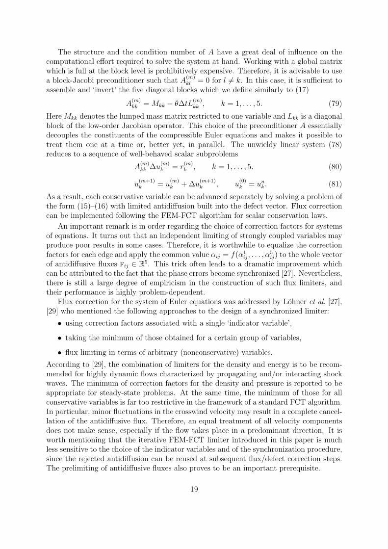
The structure and the condition number of A have a great deal of influence on thecomputational effort required to solve the system at hand. Working with a global matrixwhich is full at the block level is prohibitively expensive. Therefore, it is advisable to usea block-Jacobi preconditioner such that A

(m)kl = 0 for l 6= k. In this case, it is sufficient to

assemble and ‘invert’ the five diagonal blocks which we define similarly to (17)

A(m)kk = Mkk − θ∆tL

(m)kk , k = 1, . . . , 5. (79)

Here Mkk denotes the lumped mass matrix restricted to one variable and Lkk is a diagonalblock of the low-order Jacobian operator. This choice of the preconditioner A essentiallydecouples the constituents of the compressible Euler equations and makes it possible totreat them one at a time or, better yet, in parallel. The unwieldy linear system (78)reduces to a sequence of well-behaved scalar subproblems

A(m)kk ∆u

(m)k = r

(m)k , k = 1, . . . , 5. (80)

u(m+1)k = u

(m)k + ∆u

(m+1)k , u

(0)k = un

k . (81)

As a result, each conservative variable can be advanced separately by solving a problem ofthe form (15)–(16) with limited antidiffusion built into the defect vector. Flux correctioncan be implemented following the FEM-FCT algorithm for scalar conservation laws.

An important remark is in order regarding the choice of correction factors for systemsof equations. It turns out that an independent limiting of strongly coupled variables mayproduce poor results in some cases. Therefore, it is worthwhile to equalize the correctionfactors for each edge and apply the common value αij = f(α1

ij, . . . , α5ij) to the whole vector

of antidiffusive fluxes fij ∈ R5. This trick often leads to a dramatic improvement which

can be attributed to the fact that the phase errors become synchronized [27]. Nevertheless,there is still a large degree of empiricism in the construction of such flux limiters, andtheir performance is highly problem-dependent.

Flux correction for the system of Euler equations was addressed by Lohner et al. [27],[29] who mentioned the following approaches to the design of a synchronized limiter:

• using correction factors associated with a single ‘indicator variable’,

• taking the minimum of those obtained for a certain group of variables,

• flux limiting in terms of arbitrary (nonconservative) variables.

According to [29], the combination of limiters for the density and energy is to be recom-mended for highly dynamic flows characterized by propagating and/or interacting shockwaves. The minimum of correction factors for the density and pressure is reported to beappropriate for steady-state problems. At the same time, the minimum of those for allconservative variables is far too restrictive in the framework of a standard FCT algorithm.In particular, minor fluctuations in the crosswind velocity may result in a complete cancel-lation of the antidiffusive flux. Therefore, an equal treatment of all velocity componentsdoes not make sense, especially if the flow takes place in a predominant direction. It isworth mentioning that the iterative FEM-FCT limiter introduced in this paper is muchless sensitive to the choice of the indicator variables and of the synchronization procedure,since the rejected antidiffusion can be reused at subsequent flux/defect correction steps.The prelimiting of antidiffusive fluxes also proves to be an important prerequisite.

19

To compute the correction factors for variables other than the ones being solved for,we convert the solution differences Uj − Ui and the fluxes fij into [20]

δU ′ij := T (U)(Uj − Ui), f

′ij := T (U)fij, (82)

where T (U) ∈ R5×5 is a suitable transformation matrix. Then we invoke Zalesak’s limiter

and apply the synchronized correction factor αij to the original flux vector fij. A generalalgorithm for the construction of a flux limiter operating with an arbitrary set of quantitiesis outlined in the book by Lohner [29]. Flux limiting in terms of characteristic variablesappears to be particularly attractive. This approach has been widely used in the literatureon TVD-like methods for systems of hyperbolic conservation laws [2],[5],[38],[39].

13 Implementation of boundary conditions

The specification and implementation of boundary conditions for the Euler equations hasalways been a bit of a mystery. A comprehensive presentation of the theoretical aspectsis available in a number of popular CFD textbooks [8],[12],[42]. Boundary conditionscan be classified into physical and numerical ones. Physical boundary conditions (PBC)are required to obtain a well-posed problem, whereas numerical boundary conditions(NBC) are responsible for the stability and convergence of the algorithm. It is knownthat the tradeoff between PBC and NBC depends on the propagation properties of thehyperbolic system. If Nv is the total number of variables and Np is the number of incomingcharacteristics, then Np physical and Nn = Nv −Np numerical boundary conditions are tobe prescribed. At the inlet and outlet, Np and Nn depend on the flow regime as follows:

Inflow boundary Outflow boundarysubsonic supersonic subsonic supersonic

1D 2D 3D 1D 2D 3D 1D 2D 3D 1D 2D 3DNp 2 3 4 3 4 5 1 1 1 0 0 0Nn 1 1 1 0 0 0 2 3 4 3 4 5

At the solid wall, the normal velocity component must be set equal to zero: v · n = 0.This no-penetration or free slip boundary condition prevents the smuggling of data intoor out of the computational domain by convective fluxes.

As a rule, some or all boundary conditions are specified in terms of nonconservativevariables like the total enthalpy, entropy, pressure or deflection angle. Therefore, it isimpossible to implement them as usual Dirichlet boundary conditions. It is commonpractice to recover the desired boundary values by changing to the characteristic variables,evaluating the incoming Riemann invariants from the physical boundary conditions andextrapolating the outgoing ones from the interior of the domain [12],[42],[43]. The inversetransformation yields the values of the conservative variables at the boundary whichcan be used to compute the numerical fluxes for a finite volume method or treated asDirichlet boundary conditions for a finite difference method. Unfortunately, the extra-polation of Riemann invariants lacks a proper justification and is expensive to performon unstructured meshes. In addition, we are not aware of any publication devoted tothe implementation of characteristic boundary conditions for an implicit finite elementmethod. Let us briefly describe the simple technique we developed for this purpose.

20

In order to predict the solution values at boundary nodes, we modify the five diagonalblocks A

(m)kk of our preconditioner A(U (m)) = akl

ij by picking out the corresponding rowsand setting their off-diagonal entries equal to zero. In other words, if node i belongs tothe boundary, then akl

ij = 0, ∀j 6= i, ∀l 6= k. This enables us to update the components ofthe vector Ui = [u1,i, . . . , u5,i]

T explicitly prior to solving the linear system (80). To this

end, we simply divide the components of the nodal defect vector R(m)i = [r

(m)1,i , . . . , r

(m)5,i ]T

by the diagonal entries of the preconditioner and increment the old iterate

u∗k,i = u

(m)k,i + r

(m)k,i /akk

ii , k = 1, . . . , 5. (83)

Next, we transform the provisional solution U∗i to the vector of Riemann invariants Wi.

Recall that the number of physical boundary conditions is equal to the number of incomingcharacteristics. Therefore, we can evaluate the incoming Riemann invariants analyticallyand substitute the exact values for the predicted ones which generally do not satisfy theimposed PBC. The outgoing Riemann invariants, which are associated with the NBC,remain unchanged. Finally, we convert the modified vector W ∗

i back to the conservative

variables, assign the result to U(m)i and nullify all components of the defect vector R

(m)i .

The flow chart for the algebraic manipulations to be performed for boundary nodes beforethe solution of scalar subproblems (80)–(81) is as follows

U(m)i −→ U∗

i −→ Wi −→ W ∗i −→ U

(m)i , R

(m)i := 0. (84)

The last modification along with the fact that only the diagonal entry of row i in thematrices A

(m)kk is nonzero implies that ∆U

(m+1)i = 0 and U

(m+1)i = U

(m)i . In essence, the

corrected values U(m)i act as Dirichlet boundary conditions for the end-of-step solution.

Note that there is no need for an ad hoc extrapolation of data from the interior.In principle, all boundary conditions can be handled in this way. However, a shortcut

is feasible for the free slip condition. The predicted momentum wi = [u∗2,i, u

∗3,i, u

∗4,i]

T canbe projected onto the tangent plane without changing to the Riemann invariants:

w∗i := wi − (wi · ni)ni, (85)

where ni denotes the outward unit normal at node i. This gives the three momentumcomponents for the corrected U

(m)i , whereas the density and energy are provided by U∗

i .Yet another option is to apply the above modification to the defect for the momentumequation before computing U

(m)i := U∗

i from equation (83).

14 Numerical examples

In the remainder of this paper, we apply our iterative FEM-FCT schemes to a numberof two-dimensional test problems. The generality of the new approach makes it possibleto perform flux correction in 1D and 3D using the same postprocessing routine. Three-dimensional simulation results for bubbly flows in gas-liquid reactors can be found in [21].In the case θ = 0, our algorithm is largely equivalent to the classical FEM-FCT procedureand iterative flux correction is impractical. Therefore, we restrict ourselves to implicittime-stepping in what follows. Numerical results for the flux-corrected Lax-Wendroffscheme can be found in [17],[18]. For many more examples and a numerical analysis ofthe discretization error for our FEM-FCT methods the reader is referred to [32].

21

14.1 Solid body rotation

Rotation of solid bodies with discontinuities and small scale features is frequently used asa challenging test problem for transport algorithms. In the first example, we consider thebenchmark configuration proposed by LeVeque [26]. It is intended to examine the abilityof a numerical method to reproduce both discontinuous and smooth profiles. To this end,a slotted cylinder, a cone and a smooth hump are exposed to the nonuniform velocityfield v = (0.5 − y, x − 0.5) and undergo a counterclockwise rotation about the center ofthe square domain Ω = (0, 1) × (0, 1). Each of these bodies lies within a circle of radiusr0 = 0.15 centered at a point with Cartesian coordinates (x0, y0).

The exact solution to the pure convection equation after each full revolution matchesthe initial data depicted in Figure 3 (left). Let us introduce the normalized distancefunction r(x, y) = 1

r0

√

(x − x0)2 + (y − y0)2. It follows that u(x, y, 0) = 0 for r(x, y) > 1.Elsewhere, the reference shape of the three bodies is given by

Cylinder: (x0, y0) = (0.5, 0.75), u(x, y, 0) =

1, if |x − x0| ≥ 0.025 ∨ y ≥ 0.85,0, otherwise.

Cone: (x0, y0) = (0.5, 0.25), u(x, y, 0) = 1 − r(x, y).

Hump: (x0, y0) = (0.25, 0.5), u(x, y, 0) = 0.25[1 + cos(π min r(x, y), 1)].

The numerical solution at t = 2π produced by the iterative FEM-FCT algorithm is shownin Figure 3 (right). It was computed on a uniform mesh of 128 × 128 bilinear elementsusing the Crank-Nicolson time-stepping with ∆t = 10−3. Triangular finite elements yieldvirtually identical results [19]. No spurious wiggles come into being and the resolutionof discontinuities is remarkably crisp. Even the narrow bridge of the cylinder is nicelypreserved and the fill-in of the slot is insignificant. The inevitable ‘peak clipping’ for thecone does not exceed 10% while the hump is reproduced almost exactly. The prelimitingof antidiffusive fluxes has proved to be essential for this test. If this optional step isomitted, the sheer ridges of the cylinder are corrupted by optically disturbing kinks.

Initial data / exact solution

0

0.2

0.4

0.6

0.8

1

0

0.2

0.4

0.6

0.8

10

0.2

0.4

0.6

0.8

1

Iterative FEM-FCT, θ = 1/2.

0

0.2

0.4

0.6

0.8

1

0

0.2

0.4

0.6

0.8

10

0.2

0.4

0.6

0.8

1

Figure 3. Solid body rotation, 128 × 128 bilinear elements, t = 2π.

22

y = 0.25

0 0.1 0.2 0.3 0.4 0.5 0.6 0.7 0.8 0.9 1

0

0.2

0.4

0.6

0.8

1

y = 0.75

0 0.1 0.2 0.3 0.4 0.5 0.6 0.7 0.8 0.9 1

0

0.2

0.4

0.6

0.8

1

x = 0.25

0 0.1 0.2 0.3 0.4 0.5 0.6 0.7 0.8 0.9 1

0

0.2

0.4

0.6

0.8

1

x = 0.5

0 0.1 0.2 0.3 0.4 0.5 0.6 0.7 0.8 0.9 1

0

0.2

0.4

0.6

0.8

1

Figure 4. Cutlines for the FEM-FCT solution at t = 2π.

To examine the numerical results with extra scrutiny and facilitate comparison withthose obtained by LeVeque [26] using a TVD method, four cutlines are presented inFigure 4. The solid lines designate the analytical solution while the dots represent thenodal values of the numerical one. It can be seen that our iterative FCT limiter does areally nice job. Moreover, the results are much more accurate than those produced by theTVD method equipped with the superbee limiter which introduces too much antidiffusionand tends to steepen smooth profiles [26]. In our experience, FCT is usually superior toTVD for strongly time-dependent problems which call for the use of the consistent massmatrix. At the same time, TVD schemes are to be recommended for less dynamic flows,for which mass lumping is appropriate [22]. The optimal choice of the time-steppingscheme also depends on the dynamics of the flow. In this example, the Crank-Nicolsonmethod was selected because the fully implicit backward Euler scheme is only first orderaccurate and turns out to be diffusive at large time steps [17],[18],[19].

14.2 Rotation of a Gaussian hill

The second test case proposed by Lapin [23] makes it possible to evaluate the magnitudeof artificial diffusion due to the discretization in space and time. This can be accomplishedby applying certain statistical tools to the convection-diffusion equation

∂u

∂t+ v · ∇u = ǫ∆u in Ω = (−1, 1) × (−1, 1), (86)

where v = (−y, x) is the velocity field and ǫ = 10−3 is the physical diffusion coefficient.

23

The initial condition to be imposed is given by u(x, y, 0) = δ(x0, y0), where δ standsfor the Dirac delta function. Clearly, it is impossible to initialize the solution by a singularfunction in a practical implementation. Instead, it is reasonable to concentrate the wholemass at a single node. The integral of a discrete function over the domain Ω can becomputed as the sum of nodal values multiplied by the entries of the lumped mass matrix:∫

Ωuh dx =

∫

Ω

∑

i uiϕi dx =∑

i miui. The total mass of a delta function equals unity.Hence, one should find node i closest to the peak location (x0, y0) and set u0

i = 1/mi,u0

j = 0, j 6= i. Alternatively, one can start with the exact solution at a time t0 > 0.

In the rotating Lagrangian reference frame, the convective term vanishes and theresulting diffusion problem can be solved analytically. It can be readily verified that theexact solution of (86) is a Gaussian hill defined by the normal distribution function

u(x, y, t) =1

4πǫte−

r2

4ǫt , r2 = (x − x)2 + (y − y)2,

where x and y denote the time-dependent peak coordinates

x(t) = x0 cos t − y0 sin t, y(t) = −x0 sin t + y0 cos t.

The actual peak coordinates for a numerical approximation may be quite different.They can be calculated as the mathematical expectation of the center of mass under theprobability distribution with density uh given by the finite element solution

xh(t) =

∫

Ω

xuh(x, y, t) dx, yh(t) =

∫

Ω

yuh(x, y, t) dx.

The quality of approximation can be assessed by considering the standard deviation

σ2h(t) =

∫

Ω

r2huh(x, y, t) dx, r2

h = (x − xh)2 + (y − yh)

2,

which quantifies the rate of smearing caused by both physical and the numerical diffusion.Due to all sorts of discretization errors, σ2

h may differ considerably from the exact valueσ2 = 4ǫt. This discrepancy represented by the relative variance error

∆σrel =σ2

h − σ2

σ2=

σ2h

4ǫt− 1

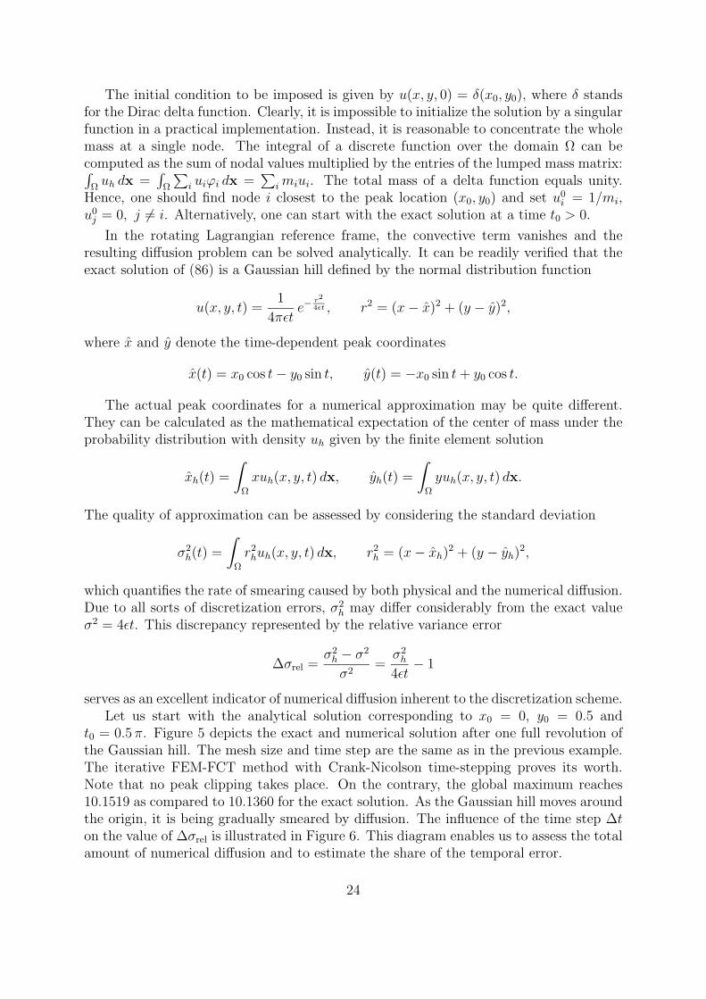
serves as an excellent indicator of numerical diffusion inherent to the discretization scheme.Let us start with the analytical solution corresponding to x0 = 0, y0 = 0.5 and

t0 = 0.5 π. Figure 5 depicts the exact and numerical solution after one full revolution ofthe Gaussian hill. The mesh size and time step are the same as in the previous example.The iterative FEM-FCT method with Crank-Nicolson time-stepping proves its worth.Note that no peak clipping takes place. On the contrary, the global maximum reaches10.1519 as compared to 10.1360 for the exact solution. As the Gaussian hill moves aroundthe origin, it is being gradually smeared by diffusion. The influence of the time step ∆ton the value of ∆σrel is illustrated in Figure 6. This diagram enables us to assess the totalamount of numerical diffusion and to estimate the share of the temporal error.

24

Exact solution, ||u||∞ = 10.1360

−1

−0.5

0

0.5

1 −1

−0.5

0

0.5

1

2

4

6

8

10

Iterative FEM-FCT, ||u||∞ = 10.1519

−1

−0.5

0

0.5

1 −1

−0.5

0

0.5

10

2

4

6

8

10

Figure 5. Rotation of a Gaussian hill, 128 × 128 bilinear elements, t = 2.5 π.

If the first-order accurate backward Euler method is employed, the temporal partof the relative variance error plays an important role at large time steps and decreaseslinearly as the time step is refined. This is also the case for the second-order accurateCrank-Nicolson scheme but the temporal discretization error is obviously much smallerthan that for the backward Euler method. As expected, the new (iterative) limiter isable to accommodate more antidiffusion than the old (non-iterative) one. In fact, ∆σrel

may even become negative if the spatial discretization error prevails. This explains theabove-mentioned enhancement of the peak in Figure 5. However, the differences betweenthe performance of the two FEM-FCT versions are marginal in the range of time stepsconsidered in this example. The Courant number must be ‘large’ for the advantages ofthe iterative approach to become pronounced. Hence, the potential of the new limitercan only be utilized to the full extent if the time derivative of the transported quantityis relatively small and temporal accuracy can be sacrificed in favor of the unconditionalpositivity offered by the fully implicit FEM-FCT method.

1 2 3 4 5 6 7 8 9 10

x 10−3

−0.5

0

0.5

1

1.5

2

2.5

3

BE/upwindBE/FCTBE/FCT (iter)CN/upwindCN/FCTCN/FCT (iter)

Figure 6. Gaussian hill: relative variance error vs. the time step.

25

14.3 Steady-state convection-diffusion

The proposed FEM-FCT algorithm can be applied to stationary problems in conjunctionwith a pseudo-time-stepping technique, whereby the steady-state solution is obtained bymarching into the stationary limit of the associated time-dependent problem. Evolutiondetails are immaterial in this case, since the time step is merely an artificial parameterwhich determines the convergence rates. Hence, it is desirable to choose time steps as largeas possible, so as to reduce the computational cost. The restrictive CFL condition preventsexplicit schemes from operating with large time steps and makes them too inefficient forour purposes. This drawback can be rectified to some extent by resorting to local time-stepping but it is obvious that steady-state problems call for an implicit treatment.

In light of the above, the fully implicit backward Euler method, which was found to bequite diffusive for transient problems, constitutes an excellent iterative solver for steadyor creeping flows. Let us investigate the numerical behavior of the BE/FCT scheme forthe singularly perturbed convection-diffusion equation

v · ∇u − ǫ∆u = 0 in Ω = (0, 1) × (0, 1),

where v = (cos 10o, sin 10o) and ǫ = 10−3. The concomitant boundary conditions read

∂u

∂y(x, 1) = 0, u(x, 0) = u(1, y) = 0, u(0, y) =

1, y ≥ 0.5,0, y < 0.5.

The solution to this elliptic problem is characterized by the presence of a sharp frontnext to the line x = 1. The boundary layer develops because the solution of the reducedproblem (ǫ = 0) does not satisfy the homogeneous Dirichlet boundary condition.

A reasonable initial approximation for the pseudo-time-stepping loop is given by

u(x, y, 0) =

1 − x, y ≥ 0.5,0, y < 0.5.

It is worthwhile to start with the discrete upwind scheme and use the converged low-ordersolution as initial data for the time-dependent FEM-FCT algorithm. This ‘educated guess’should be close enough to the steady-state limit. Hence, the computational overhead dueto the assembly and limiting of antidiffusive fluxes will be insignificant.

The numerical solutions depicted in Figure 7 were computed on a Cartesian grid of64 × 64 bilinear elements. Both of them were produced by FEM-FCT with backwardEuler time-stepping. The time step ∆t = 0.1 (Courant number ν = 6.4) was intentionallychosen to be rather large to expose the devastating effect of numerical diffusion for thenon-iterative formulation. The pronounced smearing in the vicinity of the boundary layer(see the left diagram) compromises the benefits of unconditional stability/positivity whichwere the main reason for using an implicit time discretization in the first place. Iterativeflux correction performs much better, as demonstrated by the right diagram. Both thefront and the boundary layer are resolved sharply and the solution is completely free ofoscillations. The time step must be drastically reduced (∆t ≈ 10−3, ν = 0.064) for thenon-iterative limiter to be competitive. An adaptive grid refinement makes it possibleto achieve comparable accuracy on a much coarser mesh consisting of as few as 160quadrilateral elements [19].

26

Standard limiter

0

0.2

0.4

0.6

0.8

1 0

0.2

0.4

0.6

0.8

10

0.2

0.4

0.6

0.8

1

Iterative limiter

0

0.2

0.4

0.6

0.8

1 0

0.2

0.4

0.6

0.8

10

0.2

0.4

0.6

0.8

1

Figure 7. Steady-state convection-diffusion. BE/FCT, ∆t = 0.1.

14.4 Shock tube problem

The first time-dependent example for the compressible Euler equations is the well-knownshock tube problem [24],[40]. Its physical prototype is a closed tube filled with gas whichis initially at rest and separated by a membrane into the regions of high and low pressure.Specifically, the initial conditions for the Riemann problem to be solved are given by

ρL

vL

pL

=

1.00.01.0

for x ∈ [0, 0.5],

ρR

vR

pR

=

0.1250.00.1

for x ∈ (0.5, 1].

After the membrane is removed, the flow structure in the shock tube is characterized bythree dynamically moving waves. A shock wave sets off for the region of lower pressurewith velocity vs satisfying the Rankine-Hugoniot conditions. All of the primitive variablesare discontinuous across the shock. The pressure jump propels the mass in the samedirection with velocity vp. The moving interface between the regions of different densitiesbut constant velocity and pressure represents a contact discontinuity. Finally, a rarefactionwave propagates in the opposite direction providing a smooth transition to the originalvalues of the state variables in the region of high pressure.

To compare the performance of the low-order methods based on discrete upwinding forhyperbolic systems (69) and scalar artificial viscosity (73), we present the one-dimensionalsimulation results in Figure 8. The snapshots correspond to the time instant t = 0.231.The Euler equations were discretized using 100 linear finite elements and the Crank-Nicolson time-stepping with ∆t = 10−3. The analytical solution represented by the dottedline was obtained using the technique described by Anderson [1]. Both numerical solutionsare completely free of oscillations and qualitatively correct but their accuracy leaves a lotto be desired. The smearing introduced by scalar dissipation is seen to be stronger thanthat for the finite element counterpart of Roe’s approximate Riemann solver but thedifferences are quite small. In what follows, we will stick to the former approach becauseit is more economical. In addition, some (but not too much) extra diffusion turns out tobe beneficial as long as it can be removed in the antidiffusive step [19].

27

Scalar dissipation: dij = dijI

0 0.1 0.2 0.3 0.4 0.5 0.6 0.7 0.8 0.9 1−0.2

0

0.2

0.4

0.6

0.8

1

Discrete upwinding: dij = |aij |

0 0.1 0.2 0.3 0.4 0.5 0.6 0.7 0.8 0.9 1−0.2

0

0.2

0.4

0.6

0.8

1

Figure 8. Shock tube problem in 1D. Low-order solutions, t = 0.231.

The two-dimensional results displayed in Figure 9 were computed by the iterativeCN/FCT algorithm using 128×128 bilinear elements and ∆t = 10−3. The underlying low-order method was constructed by adding scalar dissipation proportional to the spectralradius of the Roe matrix. Following the guidelines provided by Lohner et al. [27],[29], weperformed the synchronization of Zalesak’s limiter by taking the minimum of correctionfactors for the density and energy. The solution along the line y = 0.5 (see the 1D diagramin the lower right corner) demonstrates that the resolution of the shock and of the contact

Density

0 0.2 0.4 0.6 0.8 1 0

0.5

10.2

0.3

0.4

0.5

0.6

0.7

0.8

0.9

1

Velocity

0 0.2 0.4 0.6 0.8 1 0

0.5

10.1

0.2

0.3

0.4

0.5

0.6

0.7

0.8

0.9

Pressure

0 0.2 0.4 0.6 0.8 1 0

0.5

1

0.1

0.2

0.3

0.4

0.5

0.6

0.7

0.8

0.9

1

Cutline y = 0.5

0 0.1 0.2 0.3 0.4 0.5 0.6 0.7 0.8 0.9 1−0.2

0

0.2

0.4

0.6

0.8

1

Figure 9. Shock tube problem in 2D. Iterative FEM-FCT scheme, t = 0.231.

28

discontinuity is dramatically improved as compared to the low-order solutions in Figure 8.Moreover, no spurious undershoots or overshoots are observed, even though the correctionfactors for the momentum were left out of consideration in the limiting process. Due tothe fact that the time step must remain small for accuracy reasons in this example, thenon-iterative FEM-FCT method yields very similar results. However, it becomes ratherdiffusive if the minimum of correction factors for all conservative variables is employedfor synchronization. In this case, the iterative limiter performs much better because therejected antidiffusion can be built into the intermediate solution step-by-step [32].

14.5 Radially symmetric Riemann problem

The second transient benchmark was proposed by LeVeque [25] to assess the ability ofnumerical methods to preserve radial symmetry. In essence, it represents a counterpart ofthe shock tube problem in polar coordinates. Before an impulsive start, the unit squareΩ = (−0.5, 0.5)× (−0.5, 0.5) is separated by an imaginary membrane into two subregions:ΩL = (x, y) ∈ Ω : r =

√

x2 + y2 < 0.13 and ΩR = Ω\ΩL. The gas is initially at rest,whereby its pressure and density are higher within the circle ΩL than outside of it:

ρL

vL

pL

=

2.00.015.0

in ΩL,

ρR

vR

pR

=

1.00.01.0

in ΩR.

The abrupt removal of the membrane at t = 0 triggers a radially expanding shock wavewhich is induced by the pressure difference. The objective is to capture the moving shockand to make sure that the numerical solution remains radially symmetric.

The simulation results depicted in Figure 10 were obtained using the same method,mesh and time step as in the previous example. Note that the contour lines for the densityat t = 0.13 (see the left diagram) have the form of concentric circles, which demonstratesthat our FEM-FCT algorithm does preserve the symmetry. The 1D plot on the rightshows the density distribution along the x−axis for the same solution (dotted line) andfor the one computed on a much finer mesh with more than one million nodes (solid line).A good agreement is observed between the two curves. The ‘exact’ solution can be derivedby solving a one-dimensional Riemann problem with geometric source terms [25].

−0.5 −0.4 −0.3 −0.2 −0.1 0 0.1 0.2 0.3 0.4 0.5−0.5

−0.4

−0.3

−0.2

−0.1

0

0.1

0.2

0.3

0.4

0.5 Cutline y = 0

−0.5 −0.4 −0.3 −0.2 −0.1 0 0.1 0.2 0.3 0.4 0.50

0.5

1

1.5

2

2.5

Figure 10. Radially symmetric RP. Density distribution at t = 0.13.

29

14.6 Compression corner

To illustrate the potential of the fully implicit FEM-FCT algorithm for the Euler equa-tions, we apply it to a steady two-dimensional supersonic flow over a wedge which mayimitate e.g. the tip of a projectile. This standard configuration is sometimes referred toas compression corner and constitutes an excellent test problem because it can be solvedanalytically in the framework of the oblique shock theory [1]. The originally uniform su-personic flow under consideration preserves its free-stream characteristics until it reachesthe wedge which deflects it upward through an angle θ. Provided that θ is not too large,the change in the flow direction takes place across a shock wave which has the form of astraight line emanating from the tip of the wedge and running oblique to the original flowdirection. All the streamlines experience the same deflection at the shock, so that theflow behind it is also uniform and parallel to the surface of the wedge. The Mach numberdecreases, whereas the pressure, density and temperature increase across the shock wave.The so-called θ − β − M relation makes it possible to express the deflection angle θ interms of the shock inclination angle β and the upstream Mach number M1 as follows [1]

tan θ = 2 cot βM2

1 sin2 β − 1

M21 (γ + cos 2β) + 2

.

Conversely, one can determine the angle β from this formula if θ and M1 are given.In particular, the combination M1 = 2.5, θ = 15 yields a weak shock with β = 36.94.

The downstream Mach number M2 = 1.87 can be evaluated as explained in [1]. Thistest case is well documented in the CFD Verification and Validation database of theNPARC Alliance [33] where additional information and comparison data can be found.Our simulation results presented in Figure 11 were computed on a boundary-fitted meshof 128 × 128 bilinear elements and interpolated onto a Cartesian mesh afterwards forvisualization purposes. The same kind of postprocessing was employed in all the remainingexamples. Since the problem at hand is stationary, it is worthwhile to use the backwardEuler method for the discretization in time (see above). Although it is unconditionallystable for scalar equations, we had to use a moderate time step ∆t = 10−2 or a strongunderrelaxation to secure the convergence of outer iterations. It is not surprising thatour segregated algorithm for the Euler equations is insufficiently robust for steady flowswhich call for the use of a coupled solution technique [11],[41].

The distribution of Mach numbers predicted by the low-order method based on scalardissipation looks more or less reasonable (see Figure 11, top). The upstream and down-stream Mach numbers M1 and M2 are correct but the transition between them is anythingelse but discontinuous. The oblique shock is strongly smeared by numerical diffusion andactually resembles a ‘rarefaction wave’. At the same time, this overly diffusive solutionserves as a good initial guess for the FEM-FCT solver. Even the non-iterative formu-lation brings about a dramatic improvement in comparison with the low-order method.Figure 11 (middle) demonstrates that the shock is resolved sharply within 5-6 elements.However, the accuracy of the results deteriorates as the time step is increased, whereasthe iterative FEM-FCT limiter is free of this drawback. It yields the numerical solutionshown in Figure 11 (bottom), where the shock is resolved within as few as 3-4 elements.Obviously, this gain of accuracy is only recorded if the number of outer iterations issufficiently large for the rejected antidiffusion to be effectively recycled.

30

Low-order method

−1 −0.8 −0.6 −0.4 −0.2 0 0.2 0.4 0.6 0.8 10

0.1

0.2

0.3

0.4

0.5

0.6

0.7

0.8

0.9

1

Standard FEM-FCT

−1 −0.8 −0.6 −0.4 −0.2 0 0.2 0.4 0.6 0.8 10

0.1

0.2

0.3

0.4

0.5

0.6

0.7

0.8

0.9

1

−1 −0.8 −0.6 −0.4 −0.2 0 0.2 0.4 0.6 0.8 10

0.1

0.2

0.3

0.4

0.5

0.6

0.7

0.8

0.9

1

Iterative FEM-FCT

−1 −0.8 −0.6 −0.4 −0.2 0 0.2 0.4 0.6 0.8 10

0.1

0.2

0.3

0.4

0.5

0.6

0.7

0.8

0.9

1

−1 −0.8 −0.6 −0.4 −0.2 0 0.2 0.4 0.6 0.8 10

0.1

0.2

0.3

0.4

0.5

0.6

0.7

0.8

0.9

1

Figure 11. Compression corner. Oblique shock at M1 = 2.5, θ = 15.

So far we have only dealt with structured meshes, so that one of the main advantagesof the discrete FEM-FCT approach still awaits numerical verification. In order to studythe performance of the new algorithm on unstructured meshes, let us perform an adap-tive mesh refinement by clustering the grid points in the vicinity of the stationary shock.The quadrilateral elements of the coarse mesh shown in Figure 12 are successively subdi-

Figure 12. Coarse mesh with local refinement.

31

vided into four subelements which yields a computational mesh with about 10,000 verticesafter two refinements. This top-down approach enables us to generate the hierarchicalquad-tree data structures needed by our geometric multigrid solver for linear systems [41].The resulting numerical solution to the compression corner problem is shown in Figure 13.It exhibits superb accuracy and remains absolutely nonoscillatory, which confirms thatthe iterative FEM-FCT method is applicable to unstructured meshes and non-rectangularfinite elements. Furthermore, the fully implicit pseudo-time-stepping proves to be appro-priate for the steady Euler equations and an adaptive time step control [41] is feasible.It is worth mentioning that our simulation results produced by FEM-FCT appear to besuperior to the ‘reference solution’ from the NPARC database [33].

−1 −0.8 −0.6 −0.4 −0.2 0 0.2 0.4 0.6 0.8 10

0.1

0.2

0.3

0.4

0.5

0.6

0.7

0.8

0.9

1

−1 −0.8 −0.6 −0.4 −0.2 0 0.2 0.4 0.6 0.8 10

0.1

0.2

0.3

0.4

0.5

0.6

0.7

0.8

0.9

1

Figure 13. Adaptive FEM-FCT solution, M1 = 2.5, θ = 15.

14.7 Prandtl-Meyer expansion

Our last example deals with a steady supersonic flow being deflected downward ratherthan upward. In this case, the flow behavior is quite different from the one discussedabove for the compression corner. As the gas reaches the kink, it starts spreading and theflow characteristics change smoothly across the so-called Prandtl-Meyer expansion wave.The streamlines gradually bend downward and eventually become parallel to the lowerwall as they leave the rarefaction fan which separates the regions of uniform flow. Allflow properties adjust themselves continuously across the rarefaction wave except for thecritical point at which the wall geometry changes abruptly. The Mach number increases,while the pressure, density and temperature decrease. The analytical solution to thisproblem and further details can be found in the book by Anderson [1].

To comply with the NPARC setup for this benchmark [33], we adopt the free-streamMach number M1 = 2.5 and the deflection angle θ = 15. The resulting expansion fan iscomposed from an infinite number of iso-Mach lines lying in the angular sector boundedby the lines corresponding to µ1 = 23.58 upstream and µ2 = 18.0 downstream. On exitfrom the rarefaction wave, the Mach number equals M2 = 3.24 for the exact solution. Theobjective is to investigate the ability of the discretization scheme to reproduce smoothtransitions as opposed to shocks. Let us return to the settings used to obtain the resultsin Figure 11. The numerical solutions produced by the same algorithms applied to thePrandtl-Meyer expansion problem are presented in Figure 14. The numerical diffusioninherent to the low-order method (top) leads to a pronounced smearing of the expansionwave, whereas both FEM-FCT solutions (middle/bottom) are seen to be very accurate.They are virtually identical, since no flux limiting is necessary in smooth regions.

32

Low-order method

−1 −0.8 −0.6 −0.4 −0.2 0 0.2 0.4 0.6 0.8 1

−0.2

0

0.2

0.4

0.6

0.8

1

−1 −0.8 −0.6 −0.4 −0.2 0 0.2 0.4 0.6 0.8 1

−0.2

0

0.2

0.4

0.6

0.8

1

Standard FEM-FCT

−1 −0.8 −0.6 −0.4 −0.2 0 0.2 0.4 0.6 0.8 1

−0.2

0

0.2

0.4

0.6

0.8

1

−1 −0.8 −0.6 −0.4 −0.2 0 0.2 0.4 0.6 0.8 1

−0.2

0

0.2

0.4

0.6

0.8

1

Iterative FEM-FCT

−1 −0.8 −0.6 −0.4 −0.2 0 0.2 0.4 0.6 0.8 1

−0.2

0

0.2

0.4

0.6

0.8

1

−1 −0.8 −0.6 −0.4 −0.2 0 0.2 0.4 0.6 0.8 1

−0.2

0

0.2

0.4

0.6

0.8

1

Figure 14. Prandtl-Meyer expansion at M1 = 2.5, θ = 15.

15 Conclusions

An iterative FEM-FCT algorithm for multidimensional conservation laws was presented.Some deficiencies of the original formulation were exposed and measures were taken tofill the gaps. Zalesak’s limiter was embedded into a nonlinear defect correction loop. Anextension of the scalar FCT methodology to the compressible Euler equations was carriedout making use of the one-dimensional theory and flux difference splitting tools developedin the finite difference framework. The need for a proper synchronization of correction fac-tors was emphasized. An efficient way to perform the matrix assembly was proposed andother relevant implementation aspects were discussed in detail. Implicit time discretiza-tion appears to be very attractive for handling stationary problems and/or circumventing

33

the stability condition. However, our segregated approach to the solution of the Eulerequations is hardly optimal for steady flows. The convergence rates can be much improvedby using a coupled solution technique and a FMG-FAS multigrid method [11],[30]. Ananalog of the local MPSC smoother for the incompressible Navier-Stokes equations [41]seems to be a superior alternative to the commonly employed collective Gauß-Seidel re-laxation. The development of robust and efficient iterative solvers for implicit FEM-FCTschemes constitutes an important direction for further research.

References

[1] J. D. Anderson, Jr., Modern Compressible Flow, McGraw-Hill, 1990.

[2] P. Arminjon and A. Dervieux, Construction of TVD-like artificial viscosities on 2-dimensional arbitrary FEM grids. INRIA Research Report 1111 (1989).

[3] J. P. Boris and D. L. Book, Flux-corrected transport. I. SHASTA, A fluid transportalgorithm that works. J. Comput. Phys. 11 (1973) 38–69.

[4] C. R. DeVore, An improved limiter for multidimensional flux-corrected transport.NASA Technical Report AD-A360122 (1998).

[5] J. Donea, V. Selmin and L. Quartapelle, Recent developments of the Taylor-Galerkinmethod for the numerical solution of hyperbolic problems. Numerical methods forfluid dynamics III, Oxford, 171-185 (1988).

[6] J. H. Ferziger and M. Peric, Computational Methods for Fluid Dynamics. Springer,1996.

[7] C. A. J. Fletcher, The group finite element formulation. Comput. Methods Appl.Mech. Engrg. 37 (1983) 225-243.

[8] C. A. J. Fletcher, Computational Techniques for Fluid Dynamics. Springer, 1988.

[9] A. Harten, High resolution schemes for hyperbolic conservation laws, J. Comput.Phys. 49 (1983) 357–393.

[10] A. Harten, On a class of high resolution total-variation-stable finite-difference-schemes. SIAM J. Numer. Anal 21 (1984) 1-23.

[11] P. W. Hemker and B. Koren, Defect correction and nonlinear multigrid for steadyEuler equations. In: W.G. Habashi and M.M. Hafez (ed.). Computational fluid dy-namics techniques. London: Gordon and Breach Publishers, 1995, 699–718.

[12] C. Hirsch, Numerical Computation of Internal and External Flows. John Wiley &Sons, Chichester, 1990.

[13] A. Jameson, Analysis and design of numerical schemes for gas dynamics 1. Artificialdiffusion, upwind biasing, limiters and their effect on accuracy and multigrid conver-gence, International Journal of Computational Fluid Dynamics 4 (1995) 171-218.

34

[14] A. Jameson, Computational algorithms for aerodynamic analysis and design. Appl.Numer. Math. 13 (1993) 383-422.

[15] A. Jameson, Positive schemes and shock modelling for compressible flows. Int. J.Numer. Meth. Fluids 20 (1995) 743–776.

[16] D. Kuzmin, Positive finite element schemes based on the flux-corrected transportprocedure, In: Computational Fluid and Solid Mechanics, Elsevier, 887-888 (2001).

[17] D. Kuzmin and S. Turek, Flux correction tools for finite elements. J. Comput. Phys.175 (2002) 525-558.

[18] D. Kuzmin and S. Turek, Explicit and implicit high-resolution finite element schemesbased on the Flux-Corrected-Transport algorithm. In: F. Brezzi et al. (Eds.), Pro-ceedings of the 4th European Conference on Numerical Mathematics and AdvancedApplications, Springer-Verlag Italy, 2002, 133-143.

[19] D. Kuzmin, M. Moller and S. Turek, Int. J. Numer. Meth. Fluids 42 (2003) 265-295.

[20] D. Kuzmin, M. Moller and S. Turek, Implicit flux-corrected transport algorithm forfinite element simulation of the compressible Euler equations. Technical report No.221, University of Dortmund, 2002. To appear in: Proceedings of the ConferenceFinite Element Methods: 50 Years of Conjugate Gradients, University of Jyvaskyla,Finland, June 11-12, 2002.

[21] D. Kuzmin and S. Turek, Finite element discretization tools for gas-liquid flows. In:M. Sommerfeld (ed.), Bubbly Flows: Analysis, Modelling and Calculation, Springer,2004, 191-201.

[22] D. Kuzmin and S. Turek, High-resolution FEM-TVD schemes based on a fully mul-tidimensional flux limiter. To appear in J. Comput. Phys.

[23] A. Lapin, University of Stuttgart. Private communication.

[24] R. J. LeVeque, Numerical Methods for Conservation Laws. Birkhauser, 1992.

[25] R. J. LeVeque, Simplified multi-dimensional flux limiting methods. Numerical Meth-ods for Fluid Dynamics IV (1993) 175–190.

[26] R. J. LeVeque, High-resolution conservative algorithms for advection in incompress-ible flow. Siam J. Numer. Anal. 33 (1996) 627–665.

[27] R. Lohner, K. Morgan, J. Peraire and M. Vahdati, Finite element flux-correctedtransport (FEM-FCT) for the Euler and Navier-Stokes equations. Int. J. Numer.Meth. Fluids 7 (1987) 1093–1109.

[28] R. Lohner, K. Morgan, M. Vahdati, J. P. Boris and D. L. Book, FEM-FCT: combiningunstructured grids with high resolution. Commun. Appl. Numer. Methods 4 (1988)717–729.

35

[29] R. Lohner, Applied CFD Techniques. Wiley, 2001.

[30] J.F. Lynn, Multigrid Solution of the Euler Equations with Local Preconditioning. PhDthesis, University of Michigan, 1995.

[31] P. R. M. Lyra, Unstructured Grid Adaptive Algorithms for Fluid Dynamics and HeatConduction. PhD thesis, University of Wales, Swansea, 1994.

[32] M. Moller, Hochauflosende FEM-FCT-Verfahren zur Diskretisierung von konvek-tionsdominanten Transportproblemen mit Anwendung auf die kompressiblen Euler-gleichungen. Diploma thesis, University of Dortmund, 2003.

[33] NPARC Alliance, Computational Fluid Dynamics (CFD) Verification and ValidationWeb Site: http://www.grc.nasa.gov/WWW/wind/valid/

[34] S. V. Patankar, Numerical Heat Transfer and Fluid Flow. McGraw-Hill, 1980.

[35] J. Peraire, M. Vahdati, J. Peiro and K. Morgan, The construction and behaviourof some unstructured grid algorithms for compressible flows. Numerical Methods forFluid Dynamics IV, Oxford University Press, 221-239 (1993).

[36] P. L. Roe, Approximate Riemann solvers, parameter vectors and difference schemes.J. Comput. Phys. 43 (1981) 357–372.

[37] C. Schar and P. K. Smolarkiewicz, A synchronous and iterative flux-correction for-malism for coupled transport equations. J. Comput. Phys. 128 (1996) 101–120.

[38] V. Selmin, Finite element solution of hyperbolic equations. I. One-dimensional case.INRIA Research Report 655 (1987).

[39] V. Selmin, Finite element solution of hyperbolic equations. II. Two-dimensional case.INRIA Research Report 708 (1987).

[40] G. Sod, A survey of several finite difference methods for systems of nonlinear hyper-bolic conservation laws. J. Comput. Phys. 27 (1978) 1–31.

[41] S. Turek, Efficient Solvers for Incompressible Flow Problems: An Algorithmic andComputational Approach, LNCSE 6, Springer, 1999.

[42] P. Wesseling, Principles of Computational Fluid Dynamics. Springer, 2001.

[43] H. C. Yee, Numerical approximations of boundary conditions with applications toinviscid gas dynamics. NASA report TM-81265, 1981.

[44] S. T. Zalesak, Fully multidimensional flux-corrected transport algorithms for fluids.J. Comput. Phys. 31 (1979) 335–362.

36