Hierarchical Bayesian Methods For Recognition And ...€” This paper introduces a new uncertainty reasoning-based method for identiﬁcation and extraction of manufactur-ing features

IEEE TRANSACTIONS ON SYSTEMS, MAN, AND CYBERNETICS—PART A: SYSTEMS AND HUMANS, VOL. 27, NO. 6, NOVEMBER 1997 705

Hierarchical Bayesian Methods forRecognition and Extraction of 3-D

Shape Features from CAD Solid ModelsMichael M. Marefat,Member, IEEE, and Qiang Ji

Abstract—This paper introduces a new uncertainty reasoning-based method for identification and extraction of manufactur-ing features from solid model description of objects. A majordifficulty faced by previously proposed methods for feature ex-traction has been the interaction between features. In interactingsituations, the representation for various primitive features isnonunique making their recognition very difficult. We developan approach based on generating, propagating, and combininggeometric and topological evidences in a hierarchical belief net-work for identifying and extracting features. The methodologycombines and propagates evidences to determine a set of correctvirtual links to be augmented to the cavity graph representing adepression of the object so that the resulting supergraph can bepartitioned to obtain the features of the object. The hierarchicalbelief network is constructed based on the hypotheses for thepotential virtual links. The evidences which are topological andgeometric relationships at different abstraction levels impactthe belief network through their (amount of) support for dif-ferent hypotheses. The propagation of the impact of differentevidences updates the beliefs in the network in accordance withthe Bayesian probability rules.

Index Terms—Evidential reasoning, feature extraction, processplanning, solid modeling.

I. INTRODUCTION

M ACHINE identification and extraction of form featuresfrom CAD solid models is essential for many tasks

in CAD/CAM, computer vision, and manufacturing. Exam-ple tasks in these areas which need information about formfeatures include generation of process plans to produce acomponent based on its design, automatic inspection of themanufactured parts, evaluation of manufacturability of thecomponents, etc. The scheme used by most commercial CADsolid modelers to describe objects is a type of boundaryrepresentation (Brep), which uses the edges and faces bound-ing the object to describe it. However, the above-mentionedtasks commonly need and use semantic information includingdescriptions of slots, holes, pockets, etc. Form features havebeen loosely defined as a collection of topologic entities ofan object with semantic meaning. Since the form features of

Manuscript received December 22, 1993; revised October 4, 1996. Thiswork was supported in part by the National Science Foundation under Grants9210018, and 9414523 to the first author, and in part by funds provided by theDepartment of Electrical and Computer Engineering, University of Arizona.The second author was supported in part by funds from Dr. P. Lever.

The authors are with the Department of Electrical and Computer En-gineering, The University of Arizona, Tucson, AZ 85721 USA (e-mail:[email protected]).

Publisher Item Identifier S 1083-4427(97)07010-0.

an object, such as slots, holes, pockets, etc., are not directlyaccessible from the face and edge information provided by thesolid model, these form features which contain and representthe needed higher level information should be recognized andextracted from the solid model. The problem is then to generatea semantic description of the object in terms of form featuresgiven a boundary representation for it in terms of the boundingfaces and edges.

Graph-based approaches for machine interpretation of theCAD solid models to identify and extract form features hasbeen an active area of recent research [4], [11], [8], [22].One of the earliest graph-based feature extraction methodswas introduced by [11] using his Attributed Adjacency Graphs(AAG) for parts. Recognition in this method is essentiallyachieved through subgraph isomorphism. Henderson [8] pro-posed a different graph-based approach based on the assump-tion that the distinct feature subgraphs can be isolated fromtheir environs (the body graph) by detection of the cut vertexnodes. The cut vertex node represents an entrance face thatlinks a feature to the body of the part. The subgraphs separatedby cut vertex nodes represent features embedded in the originalobject. DeFloriani [4] uses a similar technique. The graphused in this technique is called the edge-face graph (EFG).The feature extraction algorithm decomposes the EFG intobiconnected and triconnected components, and the componentsare then organized into what is called an object decompositiongraph (ODG). Based on arcs incident on a component inODG, the entity is classified as a DP-feature, an H-feature,or a bridge. Sakurai and Gossard [22] proposed a techniquein which a shape feature is represented by a feature graph.A feature graph is a boundary representation graph of thefeature’s faces augmented with user fact nodes and parameternodes. Feature recognition is accomplished through graph-matching by searching the entire solid model.

A major difficulty in machine identification and extractionof form features is that form features in an object usuallyinteract with each other. Although the approaches mentionedabove and other works proposed by other researchers [7],[12], [13], [17], [27], [32] can identify instances of formfeatures when these features are isolated from each other,these methods, generally, have very limited success when thefeatures interact with each other. There are two reasons forthis difficulty:

1) Nonuniqueness: The representations for different in-stances of a particular feature are nonunique. For ex-

1083–4427/97$10.00 1997 IEEE

706 IEEE TRANSACTIONS ON SYSTEMS, MAN, AND CYBERNETICS—PART A: SYSTEMS AND HUMANS, VOL. 27, NO. 6, NOVEMBER 1997

(a1) (a2)

(b)

Fig. 1. The same representation in terms of higher level shape features and their interactions may correspond to topologically and geometricallydifferent components.

ample, while in a majority of cases all side faces of apocket are adjacent to its bottom (base) face, in manysituations one or more side faces may be disconnectedfrom the bottom face.

2) Alteration of relationships: The interaction between dif-ferent instances of form features may cause the topologicand geometric relationships between the elements of agiven feature to change. For example, one or more facesmay become divided into disconnected components, andintersecting face pairs may become disconnected once afeature interacts with a group of other form features.

The above points can be illustrated by means of a sim-ple example. Consider the simple objects (parts) shown inFig. 1(a1) and (a2). Both objects have two pockets which areperpendicular to each other, and the pocket dimensions in (a1)are identical to pocket dimensions in (a2). The representationshown in (b) represents the form features for both (a1) and(a2). Although both objects have a nearly identical semanticdescription, the topologic and geometric relationships betweenthe entities of features in (a1) and (a2) are different. In (a1),for example, all side faces (2, 3–8, 4, 5) of the vertical pocket(pocket-1) are adjacent to and intersect the base face (face-1),but in (a2) one of the side faces (side-face-3) is disconnectedfrom the base face. Similarly, other differences in topologyand geometry between the entities comprising the horizontaland the vertical pockets in (a1) and (a2) can be enumerated.

The number of classes or generic families of form featuresare limited, but the number of all their possible interactionsand the configurations in which they may appear are practicallyunlimited. To get an idea, we notice that the above two simpleexamples showed only two cases of interactions (from a set

of different possibilities) with nearly identical features bothfrom a given class. To imagine the space of possibilities, weneed to picture a multidimensional set that is a product setwhich can have any number of features, any group of differentfeature types, and any possible combination of interactions.Previous attempts have shown that is not possible to obtaingeneric patterns that can be utilized to identify all instancesof a class of form features, since the topology and geometrywhich describes the instances of a class is different for differentmembers of this product set. Another approach to overcomethe nonuniqueness, instead of searching for generic patterns,is to attempt to enumerate all sets of topologic and geometricrelationships which possibly describe instances of a givenclass of features under all different circumstances. However,such an attempt would either be impossible or exceedinglydifficult. Instead of such a brute force enumeration method, theapproach that we propose in this paper is to combine evidencesin a well defined manner to determine which features arepresent in a depression.

Evidences supporting or rejecting existence of instancesof different features can be combined to determine howdepressions of a part can be described in terms of primitivemanufacturing features such as pockets and slots. In sucha framework, each evidence may not by itself be sufficientfor recognizing a feature, but it generates a probability (ora weight), which is a measure of confidence that relates theevidence (a topologic or geometric relationship) to a feature.It is the collection of evidences and their consistent impactsupon each other that produces a description of the features.There are several important advantages to such a scheme forextracting and identifying features including:

MAREFAT AND JI: HIERARCHICAL BAYESIAN METHODS 707

Fig. 2. Schematic diagram for a simple graph partitioning approach to identify form features.

1) Since the features are recognized by the collection ofthe evidences, the individual evidences may or may notcarry equal weight, and in fact some of the individualevidences may support conflicting conclusions; as longas their cumulative combination is in favor of a correctinterpretation, a correct description of the depression willbe obtained.

2) One doesn’t need to know ahead of time which set oftopologic and geometric relationships, or which patterns,will be observed for each feature; in fact at differenttimes different topologic and geometric relationshipsmay indicate the same feature class.

3) The same topologic or geometric relationship may si-multaneously support two different features with differ-ent degrees of confidence.

The contributions of this work can be briefly summarizedas follows:

• Introducing a method to represent and model uncertainknowledge in feature recognition.

• Developing different classes of effective evidences basedon topologic and geometric relationships at differentresolution levels.

• Introducing a reasoning method based on propagation ofthe evidences in a hierarchical belief network.

• Developing an implementation of the described methodsand investigating their efficacy through experimentation.

II. GRAPH PARTITIONING

A simple graph partitioning method can be used to iden-tify and extract features correctly when form features don’tinteract or when certain simple interactions exist betweenthem. The overview of such a method can be summarizedas shown in Fig. 2. In such a method, graphs correspondingto the depressions of an object called cavity graphs canbe constructed and subsequently partitioned into templatescorresponding to generic patterns for different classes of formfeatures to obtain a set of potential features for the givendepression. Individual members of this set are then tested andeither verified or rejected using a verification procedure whichmay use a rule-based expert system, computational geometry,or another technique. In order to understand in more detailhow the method works, we present the following concepts.

Definition 1: A global graph for an object is anordered four-tuple with the followingproperties:

1) is a non-empty set of nodes of such that foreach face of the object there is exactly one node in

2) is the set of links of such that for every edgeof the object shared by two faces and there is

a link connecting the corresponding nodes in

3) : is an incidence functionthat associates with every link of an unordered pairof nodes of

4) : is a function whichlabels the links of This labeling marks a link in thegraph concave if the faces sharing the correspondingedge of the object are concavely adjacent, and marksthe link convex otherwise.

Definition 2: A cavity graph for a depression is anordered five-tuple such thatit is connected and

1) is the set of nodes of such that theunifiable nodes of are unified [16];

2) is the set of links of such thatconcave that is every link has a concavelabel;

3) : and :define the incidence function and

the link labels as before; and4) : is a func-

tion which labels the nodes of This labeling of thenodes describes the relative spatial orientation of thefaces with respect to each other in a qualitative manner[17].

A cavity graph represents the local topological informationabout a depression by means of labeled graphs. Fig. 3 (b)shows the cavity graph for one of the previous exampleobjects with two pockets which was originally shown inFig. 1. The templates for different classes or generic familiesof form features can also be encoded in terms of the locallabeled graphs described above. Fig. 4 shows the labeledgraph templates for three classes of form features, simplepockets, blind-slots, and prismatic holes (note that the facesof the features don’t need to be right-angled to each other,but their intersections may be at any angle between 0and180 ). Partitioning can subsequently be defined using graphisomorphism and graph union.

Definition 3: Isomorphism: A cavity graphand a feature template

are isomorphic denoted iff there isa bijective mapping such that

1);

2); and

3) The node labels and are consistent. Consistencymeans that either the cavity graph nodes have the samelabels as the corresponding template nodes, i.e.,

or that cavity graph node


(a) (b)

Fig. 3. Cavity graph representation for the earlier shown object with two interacting pockets.

labels are a right hand permutation of the template nodelabels.

Definition 4: Inclusion: Letand be

two cavity graphs, then is included in iff

1) and ;2) ; and3) .

Definition 5: Partition: Letbe a cavity graph, then the set of sub-

graphs of

is a partitioning of iff

1) where is some valid templateinstance (each subgraph is isomorphic to some validtemplate);

2) for (subgraphs are not included in eachother); and

3) and(the union of

the subgraphs produces the original cavity graph).

We note that the above definition allows the templateinstances forming a partition to share nodes and/or evenlinks, as long as the instances don’t include one another.The object in Fig. 5 shows the above concepts through asimple example. Fig. 5(a) shows an example object includingtwo feature instances, one pocket, oriented vertically, and oneprismatic hole oriented horizontally. Fig. 5(b) shows the onlycavity graph for this object. Fig. 5(c) shows a partitioning ofthis cavity graph which has two template instances Asimple verification procedure (either a computational geometryprocedure or a rule-based method) can subsequently be usedto verify that these two feature instances correctly describethe given object. This example illustrates an application of thesimple graph partitioning approach shown in Fig. 2.

Although this simple graph partitioning method is usefulwhen the form features of an object don’t interact or when theyinteract only in a simple manner, this method is insufficient inmore complicated situations. As an example, let us considerthe simple object which was introduced earlier in Fig. 1, andwhose cavity graph was shown in Fig. 3(b). The maximalpartitioning [17] of this cavity graph is shown in Fig. 6(a).

Fig. 4. Some families of primitive features and their cavity graph represen-tations. Faces are represented by nodes and concave adjacency relationshipsbetween faces are represented by links. Node labels are the dominant di-rections of surface normals of the corresponding faces. Other consistentpermutations ofX; Y; and B also lead to representations for the sameprimitive.

This partitioning has three template instances twoof which are isomorphic to prismatic-hole primitives and oneis isomorphic to the blind-hole primitive. Clearly this objectdoes not have two holes. As described earlier, this object hastwo pocket features (one vertical and one horizontal) openinginto each other. In order to identify and extract the two pocketsfor this part correctly, the cavity graph in Fig. 3(b) must beaugmented with two links, 3-1 and 6-2, and then correctlypartitioned. The new cavity graph produced by augmentingthe original cavity graph with these two links is shown inFig. 6(b1), and the templates which result from its partitioningare shown in Fig. 6(b2). It is clear that the two templates in6(b2) correctly identify the desired pockets in the depressionof the given part. Hence, in order to identify and extract correctdescriptions when the features interact, a more sophisticatedmethodology is needed.


(a) (b)

(g1) (g2)

(c)

Fig. 5. An example of graph partitioning. (a) shows a simple object with a vertical pocket and a horizontal prismatic hole. (b) shows the cavity graph forthe object in (a). (c) shows the partitioning of (b) which consists of two templates g1 and g2.

Fig. 7 shows a framework in which topologic and geometricevidences can be combined to determine form features of anobject. This framework is useful even when the interactionsbetween the form features makes their topology nonuniquesuch as the example discussed in Fig. 6 above. As it wasillustrated in this example, in interacting situations, becauseof the differences in topology, such as two faces beingdisconnected instead of being adjacent, etc., the cavity graphmay not include some template links (e.g., 3-1 and 6-2 above).The framework shown in Fig. 7 exploits Bayesian uncertaintyreasoning to combine evidences and explore supergraphs of theobject cavity graph(s), which are modifications of these lattergraphs. Such a method of evidential reasoning in a graph basedcontext can overcome the nonuniqueness of form features.In addition, in this framework, the generated interpretationas a whole (i.e., the collection of features) is validated forcorrectness and consistency which makes the approach morecoherent instead of only verifying individual form features.

Virtual links are the set of template links, such as 3-1and 6-2 in the above example, which are not present in thecavity graph of a depression, but whose augmentation resultsin a supergraph which is isomorphic to the union of therepresentations for the involved features. Such a supergraphcan be partitioned to obtain these features. Without the virtuallinks, these form features are not in the graph’s implicit spaceof features, and hence cannot be extracted. In general, thenumber of required virtual links as well as their identity for agiven depression are not known in advance.

Definition— Virtual Links:Suppose a depression with cavitygraph consists of the features and withthe corresponding template representations and

then the set of links of are referredto asvirtual links (provided that this set is not empty).

In the presented approach (Fig. 7), given a depression, wegenerate and combine different appropriate evidences based onthe existing geometric and topologic relationships to determinethe necessary virtual links, augment the existing cavity graphwith the determined virtual links, and then partition the result-ing graph to extract the form features. It may be necessaryto traverse the feedback loop more than once in some cases.Thus, the evidential reasoning mechanism in the feedback loopis at the core of this approach.

The form features of interest in this work are common poly-hedral machinable features like pockets, blind slots, prismaticholes, and steps. The form features used in this paper havefaces which are concave to each other, however extension tofeatures with both convex and concave relationships can beaddressed similarly. Fig. 4 showed instances of some familiesof form features considered in this research along with theirrepresentations.

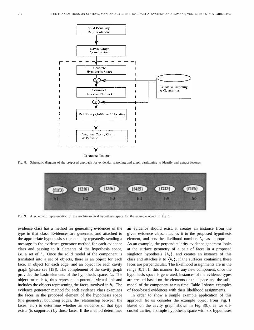
III. OVERVIEW OF EVIDENTIAL REASONING APPROACH

Fig. 8 shows the schematic diagram for the overall Bayesianevidential reasoning approach . It starts with the cavity graphfor the depression of a given part which is constructed basedon the boundary representation generated by the solid modeler.For each cavity graph, the set of links in the complementgraph, is used to obtain an initial set of potential virtuallinks. The power set of this potential set of links, that isall its subsets are used to construct an initial hypothesisspace. This hypothesis space is too large, has many unnec-essary hypotheses, and is unsuitable for efficient evidential


(g1) (g2) (g3)

(a)

(b2)

Fig. 6. An example part for which partitioning the original cavity graph will not correctly identify the form features. (a) Although the example part has twointeracting pockets, partitioning the original cavity graph generates three primitive templates(g1; g2; g3): (b) If two virtual links are added to the cavity graphin (a) the modified graph in (b1) is obtained whose partitions as shown in (b2) correctly identifies the involved form features.

Fig. 7. A frame work in which topologic and geometric evidences can be combined based on evidential reasoning to determine form features of an object.

reasoning. Therefore, based on the evidences applicable to thedepression, and based on the contradictions implied by someof the hypotheses, the initial hypothesis space is pruned toobtain a hypothesis network which is suitable for evidencegeneration, propagation, and belief updating. Evidences arepropagated through this structure and the beliefs in differenthypotheses are updated based on a Bayesian probabilisticreasoning procedure. The final belief probabilities are usedto determine the most appropriate virtual links. These virtual

links are augmented to the original cavity graph(s) and theresulting cavity graphs are partitioned to obtain the formfeatures for each depression. This process may be repeatediteratively as shown in Fig. 7 (by the feedback loop) until avalid interpretation for the object features is constructed.

IV. NONHIERARCHICAL EVIDENCE ACCUMULATION

Accumulation of topologic and geometric evidences can beused to determine the most probable virtual links for correct


identification and extraction of form features from the cavitygraphs of the object. In order to describe how this approachworks, we need to discuss i) what the involved hypothesisspace is, and how the hypotheses are generated; ii) whatevidences are, how they can be generated, and how they affectindividual hypotheses; and iii) how the effect of the evidencescan be combined to select the most probable virtual links.

A. Hypothesis Space

In order to gather and combine evidences in a formalism,a hypothesis space is needed. The objectives of constructinga hypothesis space are i) to obtain a set of hypotheses whichcomprehensively encompass the potential outcomes (in ourcase potential virtual links); ii) to develop a space which canaccept and accommodate different types of evidences; and iii)to generate a structure useful for systematic combination andpropagation of evidences.

The easiest way to construct a hypothesis space is togenerate acompleteandminimal set of potential virtual links,

The members of this set form the basic elements of thehypothesis space. For any cavity graph (recall that depressionsare modeled by cavity graphs), the elements ofcan begenerated from the links of the complement of the originalcavity graph (the complement of a graph is a graph whichhas the same nodes as the original graph but its edges arecomplement of the set of the edges of the original graph). Forour example object introduced in Fig. 1, whose cavity graphwas shown in Fig. 3(b), the six links in the complement of thecavity graph are and andform the hypothesis set where

to are individual hypotheses corresponding to the links.Therefore, if the original cavity graph is the potentialvirtual links or the links in its complement are denoted by

which can be used to produce a basic hypothesisspace. A schematic representation of the hypothesis space forthe example object introduced in Fig. 1 is depicted in Fig. 9.

B. Accumulating Evidences

A Bayesian scheme for pooling of evidences can be em-ployed to accumulate and combine evidences to select themost probable virtual links. The Bayesian-based probabilisticreasoning is a process of reasoning about partial beliefs byconditioning the probabilities of hypotheses on evidences. Inthis formalism, propositions are given numerical parameterssignifying the degree of belief accorded them under certainknowledge, and the parameters are combined and manipulatedaccording to the rules of probability theory [16]. The heart ofBayesian technique lies in the well-known Bayes rule

(1)

which states that the belief in hypothesisgiven the evidencee is observed can be computed by the product of priorprobability, and the likelihood, While theprior probability shows our belief in based on ourprevious knowledge about the likelihoodsignifies the probability that event will materialize if is

true. The likelihood represents the diagnostic or retrospectivesupport given to by the actual observed evidence. Thedenominator in (1) is a normalizing factor rendering the sumof and to unity.

Bayes rule can be extended to accommodate pooling ofseveral evidences To illustrate this point, let’s assume that asecond piece of evidence arrives. The above Bayes rule canbe applied with both evidencesand to obtain

(2)

Evidences and are very often conditionally inde-pendent given that isNow suppose we had a hypothesis space withdistinctexhaustive hypotheses, and different piecesof evidence, affecting them, and we wereinterested in ranking the hypotheses based on the combinedlikelihood indicated by these evidences. Assuming conditionalindependence, one can easily generalize (2) to obtain thelikelihood of the th hypothesis as

(3)

In (3) is constant for all hypotheses and therefore canbe factored out, thus reducing computation, when we are in-terested in ranking or clustering the hypotheses based on theirlikelihood. In situations that ratios or relationships of likeli-hoods is not enough and precise numerical values are neededmay be computed from

C. Face-Based Evidences

Evidences, which are topologic and geometric relationships,support or disconfirm the hypotheses in the hypothesis spacethrough a measure of confidence or a probability assignment.The hypothesis space is the structure which is the medium forfusion and propagation of evidences.

Face-Based Evidencesconsider particular geometry andtopology between a pair of faces (these faces must be amongthe faces associated with the elements of the hypothesis space)and relate the particular observed geometric and topologicrelationship to the possible existence of a virtual link betweenthe given pair of faces. For example, it is more probable tohave a concave intersection and hence a virtual link betweena pair of planar faces which are nearly perpendicular, thanbetween a pair of planar faces which are nearly parallel.Therefore, observation of surface perpendicularity in the CADsolid model description of the faces can be used to assign ahigher likelihood to the associated hypothesis for a virtual linkbetween them. Similarly, convexity between two faces is anevidence that strongly disconfirms the existence of a virtuallink between the involved faces.

The evidences for a hypothesis space are generated based onthe solid model description of the component. Specifically, inour implementation, there is a class for each generic evidencetype such as perpendicularity, concavity, etc., and all evidenceclasses also have a common parent, the class evidence. Each


Fig. 8. Schematic diagram of the proposed approach for evidential reasoning and graph partitioning to identify and extract features.

Fig. 9. A schematic representation of the nonhierarchical hypothesis space for the example object in Fig. 1.

evidence class has a method for generating evidences of thetype in that class. Evidences are generated and attached tothe appropriate hypothesis space node by repeatedly sending amessage to the evidence generator method for each evidenceclass and passing to it elements of the hypothesis space,i.e. a set of Once the solid model of the component istranslated into a set of objects, there is an object for eachface, an object for each edge, and an object for each cavitygraph (please see [15]). The complement of the cavity graphprovides the basic elements of the hypothesis space,Theobject for each thus represents a potential virtual link andincludes the objects representing the faces involved inTheevidence generator method for each evidence class examinesthe faces in the proposed element of the hypothesis space(the geometry, bounding edges, the relationship between thefaces, etc.) to determine whether an evidence of that typeexists (is supported) by those faces. If the method determines

an evidence should exist, it creates an instance from thegiven evidence class, attaches it to the proposed hypothesiselement, and sets the likelihood number, as appropriate.As an example, the perpendicularity evidence generator looksat the surface geometry of a pair of faces in a proposedsingleton hypothesis and creates an instance of thisclass and attaches it to if the surfaces containing thesefaces are perpendicular. The likelihood assignments are in therange [0,1]. In this manner, for any new component, once thehypothesis space is generated, instances of the evidence typesare created based on the elements of this space and the solidmodel of the component at run time. Table I shows examplesof face-based evidences with their likelihood assignments.

In order to show a simple example application of thisapproach let us consider the example object from Fig. 1.Based on the cavity graph shown in Fig. 3(b), as we dis-cussed earlier, a simple hypothesis space with six hypotheses


TABLE IEXAMPLES OF SIMPLE LIKELIHOOD ASSIGNMENTS BY FACE-BASED EVIDENCES. THE TABLE SHOWS SOME GENERIC SIMPLE

FACE-BASED EVIDENCES. THE LIKELIHOODS MAY ALSO BE FUNCTIONS COMPUTED USING PROCEDURAL ATTACHMENT

corresponding to virtual linksand can be constructed. If

we only consider the simple generic topologic evidencesshown in Table I, a total of 9 instances of evidences as theypertain to the hypotheses in this space will be generated. Eachevidence instance assigns the indicated likelihood,to thehypothesis it directly impacts, , and assigns other hypothe-ses, a 0.5 likelihood. The Bayesian method usesthe noninformative even-distribution rule (likelihood of 0.5) todistribute the impact of an evidence to hypotheses upon whichthe evidence does not directly bear. The associated likelihoodsof these evidences can be combined using (3). Fig. 10 showsthe posterior probabilities indicating the combined likelihoodfor the involved hypotheses resulting from the pooling of the9 topologic evidences. (Appendix A provides the details ofhow these posterior probabilities are computed.) It is clearfrom these results that the hypotheses corresponding to thevirtual links and are most probable and have equallikelihood. Augmenting the original cavity graph with thevirtual links and produces the modified graph shownin Fig. 6(b1). Partitioning this modified graph identifies twopockets, one with base-face 1 and side-faces 2, 3, 4, 5, andthe other with base-face 2 and side-faces 1, 4, 5, 6, as formfeatures of this object, as shown by in Fig. 6(b2).This is a correct interpretation for the example object. Wealso notice that the identified pockets of the object share 4object faces (faces 1, 2, 4, and 5).

The likelihoods in Table I are obtained by acquisition ofexpert knowledge. The expert assessments are obtained inthe qualitative form of rankings, and are then converted intonumbers which are consistent with the expert rankings. To dothis, we first consider a given evidence and determine whetherthat is an evidence which supports or disconfirms the existenceof virtual link between faces involved in the hypothesis.Subsequently, we compare that evidence with others in thesupporting or disconfirming subgroup of evidences and quali-tatively determine how it compares with each of the others inthe subgroup in strength of its support or disconfirmation. Thisprovides a qualitative distinction (supporting or disconfirm-ing), and a qualitative degree of strength (as compared with

Fig. 10. Posterior probabilities resulting from combining applicable in-stances of the simple topologic and geometric evidences for the example partin Fig. 1 using Bayesian evidence accumulation. Hypotheses correspondingto f1f3 and f2f6 are the most probable virtual links. Their addition to thecavity graph in Fig. 6(a) produces the graph in 6(b) whose partitions correctlyidentify the interacting form features (two pockets). Details of the calculationcan be found in Appendix A.

others) for each evidence. This qualitative assessment can thenbe mapped into likelihoods consistent with these assessments.For example, all supporting evidences are mapped to likeli-hoods in the range [0.5, 1]. These mappings are nonuniqueto the extent that the qualitative relationship between theevidence likelihoods are preserved, but for the purpose of theframework presented here, this is sufficient. However, it shouldalso be mentioned that the likelihoods can also be obtained bysimulation, or through optimization. In a simulation scenario,one could use a group of training examples for which thefeatures, their corresponding subgraphs, and thus the correctvirtual links are known in advance. The likelihoods are thendeveloped as weighted averages of all instances an evidence isobserved in conjunction with the hypotheses for each correctvirtual link. In an optimization scenario, one could use thegroup of training examples for which the correct virtual linksare known in advance, and find the likelihood assignmentsthrough optimizing the classification objective. This can beachieved by developing an objective function which representsthe difference between the posterior probabilities for thehypotheses corresponding to the correct virtual links and theposterior probability for all incorrect hypotheses (for the givengroup of examples), and determine the likelihood assignmentswhich optimize this objective function. This solution wouldrequire nonlinear programming to solve the optimization.

D. Limitations

One of the main shortcomings of the approach describedabove for evidence accumulation is its lack of support for


fusion of evidences at different levels of abstraction. Theevidences described in the previous section are all at a lowlevel of abstraction and are concerned with the geometricand topologic relationships between a pair of boundary faces(for generic examples of these evidences please see Table I).However, of equal or more importance are evidences that dealwith more abstract information and may exert their impact onseveral basic hypotheses. For example, a group of faces maysatisfy a set of criteria which commonly indicates the presenceof a pocket formed by these faces. Clearly, this evidencecarries higher level information concerned with (the existenceof) an entire feature, and hence this information may directlyimpact two or more basic hypotheses. A basic question in thesesituations would be how to relate or distribute the impact ofthe information upon the hypotheses.

There is no mechanism to relate or systematically distributethe effect of the abstract information upon two or morehypotheses in the above formalism. While this formalismdoes not directly support the integration of information atdifferent levels of abstraction, one may argue that an evidencesupporting two or more hypotheses, supports each hypothesisin that group, and hence one may indirectly integrate theinformation by equally supporting the individual hypothesesto the extent indicated by the evidence. Although this is apatch that may sometimes work, the obvious shortcomings arethat the same procedure cannot be followed by a disconfirmingevidence, and also that one cannot distribute the impact of theevidence in different amounts to each hypothesis.

Another major limitation of the above method is that itlacks a capability to propagate the effect of a topologic andgeometric evidence to other hypotheses which the evidencedoes not directly impact. The hypotheses in a hypothesis space,although conditionally independent, may be indirectly relatedThus, a piece of information, which as an evidence impacts ahypothesis, may also indirectly affect the certainty of anotherhypothesis. The utility of a propagation mechanism is espe-cially pronounced in fusion of information at different levels ofabstraction. For example, let us consider a hypothesis, saywhich reflects that faces and intersect, and another hy-pothesis, say which reflects that face pairs andintersect pairwise and belong to the same feature. If evidencesupports then one needs to propagate this support towhich is related to however the previous method does notprovide a systematic mechanism to render such a propagation.

One may question the significance of the propagation and in-tegration of hierarchical information limitations. The need forthese mechanisms for form feature identification and extractionis shown by the following example. The example object shownin Fig. 11(a1) has a depression with four form features. Theoriginal cavity graph for this object is shown in Fig. 11(c)by solid lines. Partitioning this original cavity graph in termsof the feature representations, will not produce a correctfeature description for the example object. We notice that,for example, face 9 and face 10 are not perpendicular to thefaces [3, 11]. The cavity graph node labels for nonorthogonalfaces are determined by the dominant components of their unitnormals as each unit normal is projected in terms of the threemajor axes (shown in the figure).

The form features of this example object can be correctlyidentified and extracted, if we augment the original cavitygraph with three virtual links, as shown by the dashed lines inFig. 11(c), to generate the modified graph, and partition it. Onecan attempt the above approach for accumulation of topologicand geometric evidences to identify the most probable virtuallinks. The complement of the original cavity graph can beused to construct a hypothesis space with 27 elements for 27potential virtual links. Fig. 12 shows the posterior probabilitiesresulting from the pooling of the instances of the topologicand geometric evidences applicable to this example object.We indirectly integrated higher level information (evidences)by equally supporting the lower level involved hypothesesto the extent proposed by the likelihood of the evidencesto obtain these results. As shown by bold type in Fig. 12,five virtual link hypotheses are determined to be the mostprobable and are equally likely. Thus, this method for poolingof evidences does not adequately recognize the three necessaryvirtual links. The results would not have been any better, ifonly the evidences impacting the lower level hypotheses areemployed, and integrating higher level information is simplyabandoned. In this latter case, the results indicate nine virtuallinks to be most probable and to be equally likely. Detailednumerical results for the latter case are not shown here becauseof space, however, we will later show that more sophisticatedmethods which can effectively fuse information from differentabstraction levels and propagate their impacts can generate acorrect form feature interpretation for this example object withthe same basic information used here.

V. SINGLY CONNECTED BAYESIAN NETWORKS

The limitations of the previous approach with integratinghierarchical information and propagating the effect of topo-logic information can be overcome by developing an approachexploiting Bayesian networks. Bayesian networks are directedacyclic graphs (DAG’s), where each node represents a setof mutually exclusive and collectively exhaustive set of hy-potheses (random variables) and the links signify probabilisticdependence (the need for conditional probabilities) betweenthe linked variables. Singly connected Bayesian networks arethose which are tree structured, that is every node except theone called root has exactly one incoming link. Ifand aretwo nodes in a Bayesian network, and they are connected bya link directed from to then is the parent of andis a child of may have other children in addition tobut in a singly connected Bayesian network, each such node

has only one parent,Fig. 13 shows a highly simplified Bayesian network. One

important feature of a Bayesian network is its explicit repre-sentation of the conditional independence among the nodes.Each node in a Bayesian network is conditionally independentof both its siblings and grandparents, given the values ofthe variables in its parents. For example, in Fig. 13, it isassumed that and and also and are conditionallyindependent given is observed. The conditional indepen-dence assumption in a Bayesian network can be regarded asa generalization of conditional independence between the evi-


(a1) (a2)

(b)

(c)

Fig. 11. (a1) and (a2) An example object with nontrivial feature interactionsand its depression. In (b), the solid lines show the cavity graph of thedepression, where [3, 11] means that two faces 3 and 11 are unified andare represented by one node. Only if the original cavity graph is augmentedwith three virtual links as shown in (c) by dashed links the form features ofthe object can be correctly identified and extracted.

dences in nonhierarchical evidence accumulation. The built-inindependence assumptions of Bayesian networks substantiallyreduce the number of needed probability parameters to specifythe probability distribution in these networks fully. Anothermajor advantage of the built-in independence assumptions istheir utility in the development of algorithms for evidentialpropagation through local computations.

Each node in a Bayesian network is associated with aquantity called “belief,” and each link is associated with aquantity called “link matrix”. The prior probability distributionfor a Bayesian network is determined by the prior beliefs forall the topmost nodes (the root nodes), and the link matrices forall links. The link matrices describe the dependency betweena node and its immediate parent(s), and relate a node to itsparent(s) using the conditional probability of the node variablegiven all possible outcomes for the parent(s). Fig. 13 shows the

Fig. 12. Posterior probabilities resulting from combining applicable in-stances of topologic and geometric evidences for the example part shownin Fig. 11 using nonhierarchical evidence pooling. This method for evidencepooling does not adequately recognize the three necessary virtual links,because five virtual link hypotheses (shown in bold) are determined as themost probable and equally likely.

fully specified prior probability distribution for our examplenetwork; is the prior probability for the only root nodeand the matrices represent the conditional probabilityof the variable given the values for all its immediate parents

In our research, each node represents a prepositional vari-able (hypothesis) with values of either true or false. With thisassumption, for the example network in Fig. 13 canbe defined as follows:

(4)

where symbols and are used to denote whether theprepositional variable (hypothesis) is true or false respectively.[In the general case, a node in a (non-singly connected)Bayesian network may have more than one parent (e.g.,parents)]. In that case, the matrix for such a noderepresents the conditional probability of given the valuesfor different possible combinations of allparents). In a singlyconnected Bayesian network, given the prior probability for theroot node and the link matrices, the prior belief for each ofthe nonroot nodes can be computed by recursively multiplyingthe belief for the parent node by the link matrix for the linkconnecting a node to its parent. For example, the prior belieffor the node in Fig. 13 is:where is a vector, and is anormalization constant such that the resulting probabilitiesin (i.e. the elements of the vectorsum up to 1. Computation of prior beliefs for nodes withmultiple parents (these types of nodes are found in non-singlyconnected networks) is more complicated. This computationcan be done by appropriate selection of cutset hypotheses and amethod called conditioning. This section is, however, focused


on singly connected networks (which don’t have such nodes),and interested readers are referred to Pearl [19] for details ofthe conditioning method.

In order to show how this type of approach for identificationand extraction of form features works, we will discuss theconstruction of hierarchical hypothesis network, the abstracttopologic evidences, and belief updating. Some example andexperimental results will show application of the method.

A. Hierarchical Hypothesis Space

Integration of information at different levels of abstractionrequires the development of a hierarchical hypothesis spacewhich can accept and accommodate various evidences atdifferent abstraction levels and combine them. In order toachieve this task, we construct a hypothesis space whichconsiders the subsets of the set of all potential virtual linksfor a cavity graph. The set of all potential virtual linksof a cavity graph may be obtained from the links in thecomplement of that cavity graph as discussed before. There-fore, if the original cavity graph is then the potentialvirtual links or the links in its complement may be denotedby and by considering all possible subsetsdenoted an initial hierarchical hypothesis space canbe constructed. In order to show a simple example, we recallthat for the cavity graph in Fig. 3(b), which corresponds tothe example object in Fig. 1, there are six potential virtuallinks, and correspondingto A diagrammatic networkrepresentation of the hypothesis space for this example isdepicted in Fig. 14. Due to limited space, not all subsets areenumerated in Fig. 14. There are subsets of

at the th level of the hypothesis space.While the hypotheses at the leaves of the hypothesis space

are single-link hypotheses, the nonleaf hypotheses are formedby the subsets of having more than one element, andthey are referred to as multilink hypotheses. The relationshipsbetween a multilink hypothesis and the single-link hypothe-ses making up its constituent elements can be modeled tobe as whole-part or cause-effect. The directed links in theconstructed hypothesis space express the dependency betweenthe linked nodes in terms of casual influence of the parentnodes on the children nodes. This causal relationship enablesus to build a Bayesian network upon these hypotheses. Theposterior probabilities for all nodes in the network obtainedfrom aggregation of different evidences will be used to decidewhich virtual links are needed for correctly identifying thefeatures of an object.

B. Network Construction

The hierarchical hypothesis space constructed as describedin the previous section should be pruned to develop a beliefnetwork. The need for this task arises from the fact thatthe described hypothesis space is too large for effectiveevidence propagation, and because this hypothesis space hasmany hypotheses which are useless or irrelevant. There are,usually, many hypotheses in the initially generated hierarchicalhypothesis space (such as that in Fig. 14) which are of no

Fig. 13. Example of a highly simplified Bayesian network. Nodes representhypotheses (or variables), and arcs represent conditional probabilities via linkmatrices. The prior probability for a Bayesian network is fully specified, ifthe prior probability for the root node(s) is given, and the link matrices arespecified.

interest. Some of the nodes in this space may even representimpossible hypotheses. For example, an interior node maycontain a hypothesis which implies an intersection betweentwo faces which are geometrically parallel. Furthermore, be-cause of the large size, employing evidence propagation in thisspace involves severe overhead in computational complexity.In order to overcome these difficulties, this hypothesis spaceshould be pruned to obtain a singly connected belief network.

To develop a suitable structure for efficient evidence gen-eration and fusion, the following constraints are followed inpruning: i) The final structure must be connected in order toallow propagation of the evidences across the network, ii) forevery evidence, there must be a node in the structure whichdirectly associates with that evidence and conveys its effect,and iii) the final structure must be singly connected.

The hypothesis space is simplified based on the assumptionthat, for a given domain, only certain subsets of areof semantic interest. For this research, the term “semanticinterest” refers to the fact that items of evidence in a problemtend to support only certain subsets of directly. We alsohowever note that enforcing condition ii) alone may not meanthat condition iii) or condition i) do hold. For example, wewill later in section E show an example (Fig. 19) in whichthe nodes which directly associate with the evidences resultin a multiconnected network (violation of condition (iii)).Therefore, we need to retain only those subsets ofwhichare of semantic interest and that they can be selected to forma singly connected Bayesian belief network. Specifically, thehypothesis space pruning is based on the following guidelines:

• A subset of (except itself) is pruned if there is noevidence bearing directly on it.

• A nonleaf subset of and its parents (except itself)are pruned if there is at least one member among itsset of hypotheses which implies an impossible geometricconstraint, such as intersection of a pair of parallel faces.

Fig. 15 shows the result of pruning the hypothesis spaceshown in Fig. 14 based on the above guidelines. The devel-oped structure is a singly connected belief network.


Fig. 14. The hierarchical hypothesis space for the example part shown in Fig. 1. The singleton hypothesesh1; h2; h3; h4; h5; andh6 represent the set ofpotential virtual links for the cavity graph shown in Fig. 3(b). The hierarchical hypothesis space consists of a total of2

6 hypotheses including the single-linkhypotheses (leaf nodes) and multilink hypotheses (the intermediate nodes). Due to limited space, not all subsets ofH at each level are shown.

C. Abstract Feature Based Evidences

One of the important advantages of the above describednetworks is that they allow fusion of abstract information.However, face-based evidences do not fully exploit the hi-erarchical nature of the hypothesis space, because they onlyinteract with the network at the leaf nodes. While the combina-tion of the face-based evidences exerting impact upon single-link hypotheses may sometimes indicate which hypothesesshould be preferred over others, the face-based evidencesby themselves may be insufficient for deciding the correctchoices, as we have shown before. Other types of evidences, towhich we collectively refer as feature based evidences, provideand integrate information which is more global and which mayencompass one or more virtual links. For example, a groupof faces may satisfy certain properties commonly found inpockets (e.g., a group of side-faces form a cycle, in whicheach side-face is concavely adjacent to two other neighboringside-faces). In this case, this information about this collectionof faces is used by a feature-based evidence to support thehypothesis for those virtual links involved in such a pocket.

Feature-based evidences may simultaneously support ordisconfirm one or more virtual links. Consequently, theseevidences may exert their impact upon the interior nodes of thehypothesis network or the leaf nodes. For instance, in terms ofthe example object from Fig. 1 with the cavity graph shown in

Fig. 3(b), the collection of faces 1, 2, 3, 4, and 5 satisfy mostproperties of pockets (including the above stated property thatevery side-face (2, 3, 4, 5) is concavely adjacent to two otherside-faces). As shown in Fig. 16(a), the subgraph representinga pocket by this collection of faces, supports the hypothesisfor a virtual link between 1, and 3. This example shows aninstance of a feature-based evidence which supports a leafnode marked in the hierarchical hypothesis network shownin Fig. 15 . While the face-based evidences are only concernedwith the geometry and topology between two faces, feature-based evidences consider and evaluate the relationships ofthose faces with their surrounding faces and edges (topologicentities) in supporting or disconfirming a virtual link between apair of faces. They represent and apply information at a higherlevel of abstraction. Feature based evidences exert their impactin a similar manner as the face based evidences through theassignment of likelihoods, to the appropriate nodes of thedeveloped belief network.

D. Belief Updating and Evidence Propagation

A variety of efficient algorithms have been developed forBayesian-based evidential reasoning and belief updating ina belief network consisting of a set of singly connectedhypotheses [9], [19], [21]. The algorithm developed by Pearl[19] is however particularly attractive. It provides an efficient


Fig. 15. The belief network resulting from pruning the hierarchical hypoth-esis space shown in Fig. 14.

and consistent means to combine evidences, to propagate theirimpacts, and to calculate the posterior beliefs for each nodein the hypothesis network.

The essence of the belief propagation and updating al-gorithm lies in its capability for propagating the impactsof evidences through local message passing. Based on thismessage passing mechanism, each node receivesmessagesfrom each of its parents (if any) and messages from eachof its children, and then updates its belief to the product ofthe two messages. For example, a nodewith parents

and children which isreceiving the combined message from its parents andthe combined message from its children, updates itsbelief to

(5)

where is a normalizing constant computed fromand encompasses the possible

values for the hypothesis If each parent sends a

message and each child sends a messagethen the combined messages are

(6)

Each node in the network will use the receivedmessages for its own belief updating and for propagation ofthe updated parameters to its neighboring nodes.

Before arrival of any evidence, each node needs to be initial-ized with prior - messages. This- message initializationin the network is dependent on the type of each node. Thereare three types of boundary nodes in a Bayesian network: theanticipatory nodes, the dummy nodes, and the root node. Aroot node is a topmost node in the network and it doesn’thave a parent and as a result itsmessage is set equal toits prior probability. An anticipatory node is a leaf node,whose prior probability has not been explicitly instantiated.For such a node, its belief, Bel, is equal to the messageit receives from its parent(s), and its message is set to 1.A dummy node represents a particular evidence bearing on anode in the network. It never receives anyor messages,but it posts a message to the node it directly bears upon.For the intermediate nodes in the network, theirmessagesare initialized to their prior beliefs and their messages areinitialized to 1.

Upon the arrival of an evidence e to a node in a network,the new information can be fused into the network by directlylinking a new dummy node representing the incoming evi-dence to the impacted node as shown in Fig. 17. The evidencenode a dummy node, posts a message to the node itdirectly impacts. The message is an estimate of(evidence

This new message starts a new propagation chainwhich for every hypothesis node in the network consists ofthree tasks of i) updating its own belief, ii) propagating the newbelief bottom up to its parent hypotheses, and iii) propagatingthe new belief top down to its other children hypotheses.

In updating its belief, when a hypothesis node receivesa new message from one of its children, or a newmessage from one of its parents, it uses equationsfrom (6) above to compute the combined andand then uses these results to compute its new belief using (5).In propagating the belief bottom up, every hypothesis nodewith a new updated belief computes and sends new messages

to each of its parents using

(7)

In propagating the belief top down, every hypothesis nodewith a new updated belief computes and sends new messages

to each of its children . These messages are computedfrom

(8)

Fig. 17 shows the complete belief propagating and updatingprocess. Each node may at any time receive new- messages


(a) (b)

Fig. 16. Two feature-based evidences for the example object in Fig. 1. In (a), the collection of faces 1, 2, 3, 4, 5 satisfy most properties for pockets, andhence, as an evidence supports the virtual link (3-1), which is part of this pocket’s representation. This evidence would supporth7 in the network of Fig. 15.Similarly, in (b), the collection of faces 1, 2, 4, 5, 6 supports the hypothesis for the virtual link 6-2.

Fig. 17. Belief propagation and updating in a singly connected network upon the arrival of an evidencee: The evidencee sends a message�e to thenode it directly impacts. Each node with a new message first updates its belief using the received messages, and then in turn sends new� messagesto its parents and new� messages to its children.

from its neighbors. If the received messages are the same as anode’s existing parameters, no action is taken. Otherwise, thisnode revises its parameters and transmits its updated messagesto its neighbors. This will cause similar revision in the neigh-boring nodes and will set up a multidirectional propagationprocess, until the network reaches its new equilibrium state.

E. An Example and Experimental Results

In this section, we will show an application of the abovedescribed approach to a nontrivial example object and discussthe implementation methods and the experimental results. Werecall that the object in Fig. 11 could not be correctly analyzedby the previous nonhierarchical techniques.

The hierarchical hypothesis space for this object has a totalof 2 elements. The complement of the original cavity graph[depicted with solid lines in Fig. 11(c)] is used to obtain theset of all potential virtual links. This set has 27 possible virtuallinks which correspond to singleton hypotheses at the leaf

nodes of the hypothesis space. The elements of the hierarchicalhypothesis space are subsets of the 27 potential virtual links.This hypothesis space is subsequently pruned to eliminatemany irrelevant and/or impossible virtual link hypotheses.

One guideline to prune the hypothesis space is to eliminatethe nodes which don’t have an evidence directly impactingthem. The face-based evidences used in this example wereinstances of the simple face-based evidences shown in Table I.While there are five generic types of face-based evidences, atotal of 37 applicable instances of these evidences were gen-erated. These evidences are directly related to the hypothesesat the leaf nodes of the network. In addition to the face-basedevidences, a total of six feature-based evidences supportingand integrating more abstract information concerning one ormore potential virtual links were also generated.

In order to find and instantiate the applicable feature-based evidences, we followed the following implementationstrategy. Different subsets of potential virtual links are added


(a) (b)

Fig. 18. The evidences support the most maximally possible (in the sense ofgraph subsumption) feature template. If the virtual link 3-1 can be supportedby both a possible pocket (a) and a possible blind-slot (b), then as long asthe pocket template subsumes the blind-slot template, we only instantiate apocket evidence.

to the original cavity graph of the object, and subsequentlythe resulting graph is searched for possible features whichcontain some of these potential virtual links. If templatesfor such features are found which contain some of thesevirtual links, then the involved group of entities (faces andedges) are checked for particular relationships which are oftenfound in a valid feature of the given template type. If theseexpected relationships exist, then an evidence is instantiated,and the appropriate likelihood assignment is made to supportthe hypothesis for the involved virtual links. The searching forthe templates is an isomorphism algorithm and is implementedas a depth-first tree-search [20].

In this implementation for generation of feature-based ev-idences, the evidences should be applied for the maximallypossible feature template. For example, as shown in Fig. 18,if a given virtual link such as (3-1), can be supported byboth a possible pocket, and a possible blind-slot, then aslong as the pocket template subsumes the blind-slot template,we only instantiate a pocket evidence. Following this aspect,prohibits multiple counting of dependent evidences that couldbe generated.

Fig. 19 shows the resulting network after pruning the initialhierarchical hypothesis space. In this network, there is acycle formed by the nodes corresponding to the hypotheses

and Since the belief propagation and updatingmethods described in the previous section are applicable tosingly connected networks, they cannot be directly appliedto fuse the topologic and geometric evidences in this net-work. In order to exploit the described hierarchical approach,the network in Fig. 19 can be approximated by the singlyconnected network shown in Fig. 20. The main differencebetween the network in Fig. 19 and its singly connectedcounterpart is that node is replaced by its immediateparent providing both and the parent node a propagationpath to the child node without a cycle. We will discusshandling cycles and approximating multiconnected networksby singly connected networks further in the next section. Allthe evidences applicable to the network in Fig. 19 can also beapplied to the singly connected network in Fig. 20.

Appendix B shows the final results of evidence propagationand belief updating by combining the applicable topologic andgeometric evidences for all hypothesis nodes of the networkin Fig. 20. This network has 32 hypotheses and is four layersdeep. As shown by bold type in the results presented in the

appendix, the hypotheses for the three virtual linksand are the most probable links.

Addition of these links to the original cavity graph producesa modified graph isomorphic to that shown in Fig. 11(c), andits partitioning identifies the correct four form features ofthis object. Fig. 21 shows the results of the extracted featuresand the partitioning. These results correctly identify that theexample object contains three pockets, one with the base-face1 and side-faces 2, 7, 6, 8, another with base-face 5 andside-faces 1, 2, 4, 3, and the third with the base-face 7 andside-faces 1, 3, 4, 6, and a prismatic hole with faces 10, 1, 4,9. The generated feature descriptions can be verified againstthe detailed solid model description of the correspondingdepression (through a volumetric check) for correctness andconsistency.

Although the three links needed to correct the cavity graphand get correct results based on partitioning are the threemost probable virtual links, , and , there is nonode in the pruned hypothesis network (Fig. 20) that containsthese three virtual links and only these virtual links. Thereason is that there is no evidence that directly supports thehypothesis node with all these three links, and only thesethree links. The current pruning heuristics prune those nodescorresponding to virtual link sets which i) are not directlysupported by any evidence, and ii) are not necessary forgenerating a singly connected belief network. As a result thenode having these three links gets pruned during the pruningstep. The evidential supports for the three virtual links comefrom different evidences. Different evidences support differentsubsets of these virtual links (in addition, some evidencessupport virtual links other than these three). For example asshown in the resulting network of Fig. 19, there is evidencedirectly supporting the virtual link set thereis evidence directly supporting the set and there isalso evidence directly supporting the set amongothers.

In augmenting the cavity graph with virtual links, twotechniques are possible. The first technique adds the virtuallinks associated with the most probable beliefs one at a time tothe cavity graph, and analyzes the resulting structure to find outwhether a correct interpretation of the object’s depression canbe generated (the interpretation generated through partitioningcan be volumetrically checked against the solid model of theobject). If a correct interpretation of the object is not ob-tained, the resulting structure is augmented with the next mostprobable virtual link, and so on. In the second technique, aclustering method can be used to cluster the virtual links basedon the posterior probability associated with their hypotheses.Subsequently, all the links belonging to the highest rankedcluster are employed. We used the first technique in the aboveexperiment. Thus, the modified graph with the three necessaryvirtual links is generated by stage-wise addition of the mostprobable links. (This obviated the need to knowa priori thequantity of the links and the clustering need.)

This example and the experimental results demonstratehow an application of the described hierarchical approach forcombining and propagating topologic and geometric evidencescan be used to generate the form features from the solid model


Fig. 19. The multiply connected belief network for the more complicated part shown in Fig. 11. The leaf nodes represent the single-link hypotheses.

Fig. 20. A singly connected network approximation for the multiply connected belief network shown in Fig. 19.

Fig. 21. The features recognized for the example object in Fig. 16 bypartitioning (a).

of an object automatically. This could not be handled correctlyby the earlier introduced nonhierarchical approach, or by graphpartitioning alone (as in Fig. 2).

VI. M ULTICONNECTED NETWORKS

The previous sections showed that hierarchical fusion andpropagation of topologic and geometric evidences can beuseful for machine understanding of the CAD solid model ofmany parts, but we also noticed that the developed hypothesisspace is multiconnected (i.e. it contains cycles) in many cases.For example, the generated hypothesis network in the previous

experiment (Fig. 19) had a cycle consisting of hypothesesand When cycles occur in the hypothesis

network, the previous methods are no longer useful for tworeasons. Firstly, because of the cycles, the propagation ofbeliefs between the hypotheses may never terminate. Sec-ondly, and most importantly, the cycle existence implies thatthe necessary conditional independence assumptions betweenthe hypotheses (specifically between siblings and betweengrandparent/grandchild nodes) are not satisfied in the network.

The method used in the last section to generate a solutionfor the developed hypothesis network of Fig. 19 exploitsapproximating the network with a singly connected networkthus avoiding the problems with the cycles. However, approx-imation by a singly connected network does not allow allevidences to be applied to the hypotheses which are directlyrelated to them, instead some of the applicable evidences canonly insert their impact on other somehow related hypotheses.In addition, because the network topology is manipulated, thefusion of the topologic and geometric evidences provides onlyan approximation to the resulting belief in the hypotheses. Inthis section, we present an approach based on multiconnectednetworks, to solve the problem in these situations effectively.


A. Hypothesis Space and Network Construction

The hypothesis space can be generated by the same methodas the hypothesis space in the previous section for the singlyconnected Bayesian networks. In order to develop a beliefnetwork, the generated hypothesis space is pruned, and asbefore, the main approach here is to keep the hypotheses whichare of semantic interest. However, in constructing the network,we relax the constraint that the final structure must be singlyconnected.

B. Approach to Aggregating Topologicand Geometric Evidences

It is known that the general problem of updating belief inan arbitrary multiconnected network is NP-hard [2]. However,because the number of nodes in this work is in the order of tens(much smaller as compared with thousands of nodes in medicalapplications), the necessary computations don’t pose a seriousproblem. We exploit a technique based on blocking some ofthe broadcast pathways to fuse and propagate topologic andgeometric evidences in networks which have cycles. Blockingthe pathways prevents cycling of messages in the cycles. Thistechnique uses the method of belief conditioning [19]. In orderto block the desired broadcast pathways, the value of someof the hypothesis nodes called cutset nodes is assumed to beknown. The belief in these cutset nodes is calculated duringthe initialization process of the network. Subsequently, thebelief in the cutset hypotheses doesn’t change during the beliefpropagation process, since their value is assumed known andthe amount of belief in them is known. Therefore

1) cutset nodes don’t pass messages from their parents totheir children, and

2) cutset nodes don’t pass messages from one child to anyother children.

This aspect allows the belief in all other hypotheses to becomputed via message propagation as it was done before.The final belief in each network hypothesis is obtained bycombining the derived beliefs for that particular hypothesisfrom each assumed value of the cutset hypotheses.

Let us consider our previous multiconnected hypothesisnetwork example of Fig. 19 to demonstrate how this techniqueworks. Although the computation process for the completenetwork follows identical steps, we will concentrate on the leftpart of the hypothesis network which is redrawn in Fig. 22(a)to simplify discussion. Assume that represents a set ofevidences applicable to the hypotheses in thisnetwork. From the law of total probability, the belief in anyhypothesis, in the network can be calculated from

which is equivalent to

(14)

Equation (14) shows that the belief in any hypothesiscanbe computed as the weighted average of the belief conditionedupon the possible values of The weighting factors are thebelief in individual values (outcomes) of This equationcorresponds to using as a cutset node and thus conditioningthe belief in other hypotheses upon its assumed value. In theabove discussion, we used as the cutset node to blockcycling of the messages in the cycle for our example, however,the same technique can also be applied withor insteadof

With the belief in known, and no broadcast from oneneighbor to another neighbor through the belief in otherhypotheses, and are computedthrough a message propagation mechanism similar to the onedescribed earlier. The posterior probabilities, and

are obtained fromThe major differences here are in the process to initialize thepruned network, and in computing the weighting factors.

C. Network Initialization

There are a number of major differences in the initializationprocess in order to combine topologic and geometric infor-mation. The initialization tasks to be achieved are i) to selectthe cutset hypotheses to block the cycles, ii)to calculate the prior beliefs for the nonroot hypotheses, andiii) to compute the joint probability for the cutset hypotheses.

In the belief propagation process, since change in the beliefof any one of the neighbors of (the cutset node) does notaffect its belief and thus the and messages supplied toother neighbors, it is as though each neighbor of the cutsetnode has its own private copy of the node with which itinteracts. Fig. 22(b) demonstrates the situation graphically,which holds in general for the cutset nodes and their neighbors.Suppose are the cutset hypotheses and that

denote an outcome combination or outcomevalue for these hypotheses. Then the weighting factors areequal to for eachpossible combination of values For binary hypothe-ses, there are only two values of true and false forTheweighting factors are obtained from

(15)

where is a normalizing constant obtained from

The first term in (15), towhich for simplicity we refer as cannot bedirectly obtained. Therefore, it is computed using the chainingconditional probability method suggested by [3]

(16)


(b)

Fig. 22. (a) The left part of the belief network of the example in Fig. 19.There is a cycle between the hypothesis nodesh0; h2; h8; and h3: (b) Ifh0 is used as a hypothesis cutset node it blocks the pathways through itas if each neighboring node had its own private copy of this node; (b) alsoshows propagating the prior beliefs as part of computing the weighting factorsBEL(h0) andBEL(:h0) and initializing the network.

In order to compute the joint probability using (16), thecutset hypotheses are instantiated in the network in a sequentialorder such that computing the prior probability ofdoes notrequire an instantiated value for that is none ofthe hypotheses whose value is among this latter group is apredecessor of Subsequently, the prior belief of the rootnodes can be propagated through the network (using the linkmatrices) to recursively obtain etc.

After sequentially instantiating the cutset hypotheses, wecan calculate the prior beliefs for other hypotheses

by propagation throughthe link matrices. For example, for a nodewith parentsand we compute ’s prior belief as follows:

(17)

where are the possible outcomes of andFig. 22(b) shows the propagation of beliefs for initialization

in our example network in which is the only cutsethypothesis.

D. Accumulation and Propagation of Geometric Evidences

The major difference in fusion of topologic and geomet-ric evidences is that a new set of weighting factors are

computed with every new evidence. The set of weightingfactors are calculated using (15). We have described howthe first joint probability term is obtained in the previousinitialization section. For every new evidence the secondterm can be calculatedin a recursive fashion from the previous set of conditionalbeliefs

By attaching a dummy evidence node with tothe network and propagating the current beliefs through thelink matrix to this node, we can compute

Thus every evidence in itsturn uses the weight factors from the previous evidence tocompute

(18)

which will then be used to compute the new set of weightfactors. Fig. 22(b) shows the propagation of the messagesto the evidence node eto determine the weight factors,

andThe effect of each topologic and geometric evidence is

propagated in the constructed belief network by a similartechnique as for the singly connected networks to obtain

After the newweight factors are computed, each new evidence node posts a

message to its parent hypothesis node. This new messagestarts a new propagation chain which for every hypothesisnode in the network consists of three tasks of i) updatingits own belief, ii) propagating the new belief bottom up toits parent hypotheses, and iii) propagating the new belieftop down to its other children hypotheses. This method canpropagate the evidences and update the belief in the hypothe-ses, because the pathways containing cycles are blocked bythe cutset hypotheses whose outcomes and whose beliefs areknown.

E. Example and Experimental Results

Let’s again consider the example network of Fig. 19 whichcorresponds to the object with the complex depression shownin Fig. 11 to demonstrate the application of the method.There are 27 potential virtual links for this example object.37 instances of the geometric evidences are automaticallygenerated including 27 face-based evidences and five feature-based evidences. The belief network in Fig. 19 constructedafter pruning the hypothesis space has 32 hypotheses. Thepreviously discussed approaches could produce a solutionfor this object only if the original network is approximatedwith a singly connected network. The described conditioningapproach to block certain broadcast pathways can be exploitedwithout the need to approximate the network.

Appendix C shows the results for combined beliefs fromaccumulating and propagating the geometric and topologicevidences using the described conditioning method. The hy-pothesis h is used as the only necessary cutset hypothesis


to break the cycle present. Hypotheses and are themost probable hypotheses, as posterior probabilities indicate(shown by bold). These hypotheses correspond to the virtuallinks and Hence the aggregate of the topo-logic and geometric evidences indicate that these three virtuallinks should be augmented to the cavity graph previouslyshown by solid lines in Fig. 11(c). The resulting graph is thenused to identify and extract instances of the form features.

Considering the example object of Fig. 11, we notice thatnonhierarchical Bayesian approach cannot identify the threenecessary virtual links for correctly identifying and extractingthe involved form features. This approach identifies five linksincluding two incorrect links and as equally mostlikely. The method based on hierarchical singly connectedBayesian networks can identify the three necessary links,but it approximates the original network, and thus may notprovide comparative likeliness as accurately. An advantage ofthe approach using the multiconnected network is that all ofthe evidences can be directly applied to the hypothesis nodeswhich they directly bear upon.

VII. CONCLUDING REMARKS

In this paper, we have described an approach based on thegeneration and combination of evidences exploiting Bayesianprobabilistic propagation to identify and extract features froma part’s solid model representation. The method works byconstructing a graph which combines the original cavity graphrepresenting the depression with a set of virtual links, andsubsequently partitioning this resulting graph to obtain thepart’s features. However, the essence of the approach is infinding the set of correct and necessary virtual links. Theevidences, which are geometric and topologic relationshipsat different levels of abstraction, are applied and propagatedthrough a hierarchical hypothesis network for potential virtuallinks. The impact of each evidence is a measure of confidence(or probability) which causes the beliefs in all hypothesisnodes of the network to be updated after arrival of thatevidence. The methods for updating these beliefs are inaccordance with Bayesian probability rules.

The main contributions of this research work can be sum-marized as introducing a method to represent and modelknowledge with uncertainty in feature recognition, developingdifferent classes of evidences based on the geometric and topo-logic relationships at different abstraction levels for effectivereasoning, and introducing a reasoning method based on thepropagation of the evidences in a hierarchical belief network.These methods are developed to help with the nonuniquenessof shape feature descriptions in different interactions which

has been one of the hindrances in automated identificationand extraction of shape features from CAD solid models.The proposed methods can successfully extract the interactingfeatures for many parts, however, much work still remainsto be done. One immediate goal for us is to generalize thedeveloped methodology to identify and extract features withcurved surfaces from components with nonplanar surfaces.

APPENDIX AEXAMPLE COMPUTATION OF

POSTERIOR PROBABILITIES IN FIG. 10

The following shows how the posterior probabilities arecomputed for the example in Fig. 10.

Then

Then, where (see the bottom of thepage) so

APPENDIX BBELIEF PROPAGATION RESULTS FOR THEEXAMPLE OF FIG. 20

The following shows the final results of evidence propaga-tion and belief updating by combining the applicable topologicand geometric evidences for all hypothesis nodes of thenetwork in Fig. 20. The network of Fig. 20 has 32 hypothesesand is four layers deep. As shown by the bold type, the

and


hypotheses for the three virtual links and arethe most probable links.

Likelihoods 1: if feature evidence involves onevirtual link; if feature evidence involves severalvirtual links.

Likelihoods 2: if feature evidence involves onevirtual link; if feature evidence involves severalvirtual links. (See table at the bottom of the page.)

For the abstract feature evidences, we used two differentlikelihood setups for the feature evidences. Likelihood setup 1used a likelihood, of 0.9 if the feature evidence involvedonly one virtual link, and used 0.6 if the feature evidenceinvolved several links. Likelihood setup 2 used a likelihood,

of 0.8 if the feature evidence involved only one virtuallink, and used 0.65 if the feature evidence involved severallinks. In assigning likelihoods, the strategy was that there isless confidence in evidences for a feature whose representationis farther from its expected template (that is if more thanone virtual link is involved in the potential feature template,less support is accorded to that feature, and the corresponding

hypothesis). However, by experimenting with two differentlikelihood setups, we note that the rankings of posteriorprobabilities don’t change. For our purposes, the exact value ofthe numbers resulting from the combination of the evidences isnot so important because conclusions regarding the hypothesesare drawn based on the rankings and relationships of thebeliefs in different hypotheses, not the exact value of the beliefnumbers. Great precision is not necessary in these parameterassignments.

APPENDIX CBELIEF PROPAGATION RESULTS FOR

THE MULTICONNECTED NETWORK

The following shows the final results of posterior prob-abilities using conditioning for all hypothesis nodes of themulticonnected network of Fig. 19 which contains a cycle.Hypothesis h has been used as the cutset hypothesis. Thehypotheses for the three virtual links and arethe most probable links. Comparing these results with those

Hypothesis Virtual Link(s) Posterior ProbabilitiesLikelihoods 1 Likelihoods 2

all potential virtual links


Hypothesis Link Posterior Probabilitiesthe original hypothesis sets 0.00(1,8), (3,5) 0.81(4,7), (6,9) 0.73(6,9), (6,10) 0.65

0.01(1, 8) 0.94(3, 5) 0.94(4, 7) 0.94(6, 9) 0.82(6, 10) 0.73(1, 4) 0.03(2, 3) 0.03(2, 6) 0.02(2, 7) 0.09(2, 8) 0.09(2, 9) 0.09(2, 10) 0.09(3, 6) 0.03(3, 9) 0.10(3, 10) 0.10(4, 8) 0.11(5, 6) 0.11(5, 7) 0.02(5, 8) 0.03(5, 9) 0.03(5, 10) 0.02(7, 8) 0.03(7, 9) 0.03(7, 10) 0.02(8, 9) 0.02(8, 10) 0.03(9, 10) 0.03

in Fig. 21 obtained from a singly connected approximationshows an improvement. (See table at the top of the page.)

REFERENCES

[1] E. Charniak, “Bayesian network without tears,”AI Mag., vol. 12, no.4, 1991, pp. 50–63.

[2] G. F. Cooper, “The complexity of probabilistic interference usingbayesian belief networks,”Artif. Intell., vol. 42, pp. 293–405, Mar.1990.

[3] M. R. Chavez and G. F. Cooper, “A randomized approximation al-gorithm for probabilistic inference on Bayesian belief networks,”Net-works, vol. 20, no. 5, pp. 661–685, 1990.

[4] L. DeFloriani, “Feature extraction from boundary models of 3-D ob-jects,” IEEE Trans. Pattern Anal. Machine Intell., vol. 11, no. 8, pp.785–798, 1989.

[5] A. P. Dempster, “A generalization of Bayesian inference,”J. Royal Stat.Soc., vol. 30, pp. 205–247, 1968.

[6] J. Gordon and E. H. Shortliffe, “A method for managing evidentialreasoning in a hierarchical hypothesis,”Artif. Intell., vol. 26, no. 3, pp.323–357, 1985.

[7] M. R. Henderson, “Computer recognition and extraction of form fea-tures: a CAD/CAM link,” Comput. Industry, no. 5, pp. 329–339,1984.

[8] M. R. Henderson, S. H. Chuang, and G. P. Gavankar, “Graph-basedfeature extraction,” inProc. NSF Design Manufacturing Systems Conf.,Tempe, AZ, 1990.

[9] M. Henrion, “An introduction to algorithms for inference in belief nets,”in Uncertainty in AI. Amsterdam, The Netherlands: North-Holland,1990, pp. 129–138.

[10] E. J. Horvitz, J. S. Breese, and M. Henrion, “Decision theory in expertsystems and artificial intelligence,”Int. J. Approximate Reasoning, vol.2, pp. 247–302, 1988.

[11] S. B. Joshi and T. C. Chang, “Graph-based heuristics for recognition ofMachined Features from a 3-D solid model,”Comput. Aided Des., vol.20, no. 2, pp. 58–66, 1988.

[12] H. Kung, “An investigation into development of process plans fromsolid geometric modeling representation,” Ph.D. dissertation, OklahomaState Univ., Oklahoma City, 1984.

[13] L. K. Kyprianou, “Shape classification in computer-aided design,” Ph.D.dissertation, Univ. Cambridge, Cambridge, U.K., 1980.

[14] S. L. Lauritzen and D. J. Spiegelhalter, “Local computations withprobabilities on graphical structure and applications to expert systems,”J. Royal Stat. Soc. B, vol. 50, no. 2, 1988.

[15] M. Marefat, S. Malhotra, and R.L. Kashyap, “Object oriented intelligentcomputer integrated design, process planning, and inspection,”IEEEComput., vol. 26, no. 3, 1993.

[16] M. M. Marefat and R. L. Kashyap, “Geometric reasoning for recogni-tion of three dimensional object features,”IEEE Trans. Pattern Anal.Machine Intell., vol. 12, no. 10, 1990.

[17] , “IDP: Automating the CAD/CAM link by reasoning aboutshape,” in Proc. 6th Conf. Artificial Intelligence Applications, SantaBarbara, CA, 1990.

[18] N. J. Nilsson, Principles of Artificial Intelligence. Palo Alto, CA:Morgan Kaufmann, 1980.


[19] J. Pearl,Probabilistic Reasoning in Intelligent Systems. Palo Alto, CA:Morgan Kaufmann, 1988.

[20] S. M. Olmsted, “On representing and solving decision problems,” Ph.Ddissertation, Dept. Eng. Economic Syst., Stanford Univ., Stanford, CA,1983.

[21] M. A. Peot and R. D. Shachter, “Fusion and propagation with multipleobservations in belief networks,”Artif. Intell., vol. 48, no. 3, pp.299–318, 1991.

[22] H. Sakurai and D. C. Gossard, “Recognition shape features in solidmodels,” IEEE Comput. Graphics Applicat., vol. 10, no. 5, pp. 22–32,1990.

[23] G. A. Shafer,Mathematical Theory of Evidence. Princeton, NJ: Prince-ton Univ. Press.

[24] G. Shafer, “Probability judgment in artificial intelligence and expertsystem,”Statist. Sci., vol. 2, no. 1, pp. 3–44, 1987.

[25] G. Shafer and J. Pearl,Uncertain Reasoning. San Mateo, CA: Morgan-Kaufmann, 1990.

[26] P. P. Shenoy and G. Shafer, “Propagating belief functions with localcomputations,”IEEE Expert, vol. 1, no. 3, pp. 43–52, 1986.

[27] S. M. Staley, “Using syntactic pattern recognition to extract featureinformation from a solid geometric data base,”Comput. Mech. Eng.,vol. 2, no. 2, pp. 61–66, 1983.

[28] D. A. Stratton and R. F. Stengel, “ Probabilistic reasoning for intelligentwind shear avoidance,”J. Guidance, Contr., Dynamics, vol. 15, no. 1,pp 247–254, 1992.

[29] S. N. Trika,, “Detection of virtual links by geometric reasoning andfeature extraction based on modified cavity graphs,” Dept. Elect. Eng.,Purdue Univ., West Lafayette, IN, Mar. 1992.

[30] J. R. Ullman, “An algorithm for a subgraph isomorphism,”J. ACM,vol. 23, no. 1, pp 31–42, 1976.

[31] X. Yang, and D. Okrent, “A diagnostic expert system for helping theoperation of hazardous waste incinerators,”J. Hazardous Materials, vol.26, 1991, pp. 27–46.

[32] T. C. Woo, “Feature extraction by volume decomposition,” inProc.Conf. CAD/CAM Technol. Mech. Eng., Mass. Inst. Technol., Cambridge,1982.

Michael M. Marefat (S’89–M’89) received theB.S. degree in electrical and computer engineeringand the B.A. degree in mathematical sciences fromRice University, Houston, TX, in 1986. He receivedthe M.S. and Ph.D. degrees in electrical engineeringfrom Purdue University, West Lafayette, IN, in 1988and 1991, respectively.

He is the Director of the Knowledge Systems En-gineering Laboratory and a Faculty Member in theDepartment of Electrical and Computer Engineeringat the University of Arizona, Tucson. He has been

involved in research in the areas of knowledge-based systems, visualization,computer graphics, machine vision, and CAD for the last ten years. He is theauthor or co-author of about 100 refereed research articles. His research hasbeen supported by the National Science Foundation and by NASA. He hasbeen the supervisor of more than 12 masters theses and Ph.D. dissertations. Hisprevious experience includes Schlumberger Laboratory for Computer Science,Purdue Engineering Research Center for Intelligent Manufacturing Systems,and Baylor Digital Imaging Laboratory.

Qiang Ji received the B.S. degree in materials engineering in 1984 fromthe Shaan Xi Polytechnic University, China. He has received three M.S.degrees: in mineral engineering from the University of Alabama, Tuscaloosa,in electrical engineering from the University of Alabama, both in 1991, andin electrical engineering from the University of Arizona, Tucson, in 1993.

He is now a Research Engineer with the Western Research Company in-volved in developing imaging and pattern recognition algorithms for biomed-ical applications. He is a principle investigator for an NIH-funded projectfocused on developing algorithms for automatically classifying human tis-sues using texture analysis and pattern recognition techniques. His researchinterests include image processing, computer vision, pattern recognition, andneural networks.

Documents

Hierarchical Bayesian Methods For Recognition And ...€” This paper introduces a new uncertainty reasoning-based method for identiﬁcation and extraction of manufactur-ing features