Embed Size (px)
Citation preview

HF PROPAGATION Results : Metal
Oxide Space Cloud (MOSC)
Experiment
Dev Joshi
Research Assistant
Department of Physics, Boston College(BC)
Institute For Scientific Research(ISR), BC
ISR SEMINAR
1
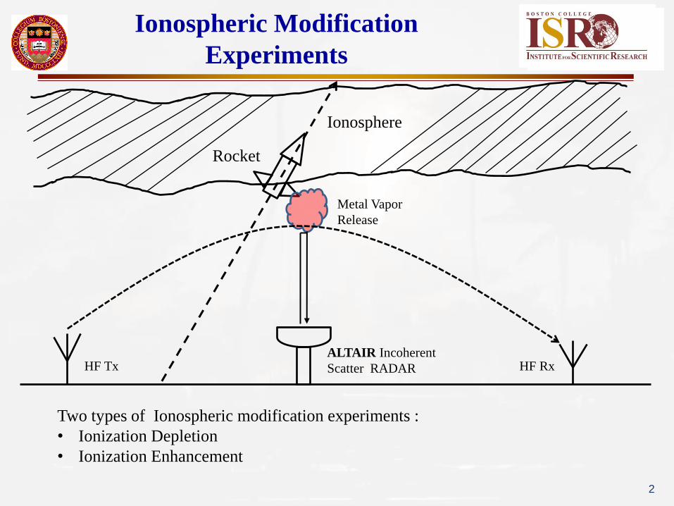
Ionospheric Modification
Experiments
HF Tx HF Rx ALTAIR Incoherent
Scatter RADAR
Metal Vapor
Release
Rocket
Ionosphere
Two types of Ionospheric modification experiments :
• Ionization Depletion
• Ionization Enhancement
2

HF PROPAGATION Results : Metal
Oxide Space Cloud Experiment
Outline : • Introduction
• Ionosphere Modification
Experiment
• HF propagation in ionosphere
• Observations
• Modeling Results
• Conclusions
3

Ionospheric Modification
Experiments
Ionospheric Modification Experiments: Various materials have been injected
into the high atmosphere creating perturbations to the ambient medium.
• To detect plasma drift velocities and electric fields.
• To create artificial comets.
• To exploit the ionosphere and magnetosphere as a plasma
laboratory without walls.
• To increase or decrease the plasma density in the
ionosphere to trigger large scale phenomenon.
• Payload for each rocket included
‒ Two canisters of samarium
(5 kg yield)
‒ Dual Frequency RF Beacon
(NRL CERTO)
• Ground diagnostics from 5 sites included:
‒ ,GPS/VHF
Scintillation Rxs, All-Sky Cameras,
Optical Spectrograph, Ionosondes,
Beacon Rx,
Incoherent Scatter Radar
HF Tx/RX 4

Ionization Depletion Chemistry
• H2O, H2, SF6
• An example with water and hydrogen molecules
Ionization Enhancement
• Barium, Strontium, Xenon, Lithium, or Cesium: Photoionization
• Lanthanides: Photoionization and Chemi- ionization
Ionization Depletion and
Enhancement
These panels show pre-event conditions (a) and the resultant
perturbations at 14 minutes (b), 40 minutes (c), and 107 minutes (d)
after the Shuttle thruster firing in Space Lab 2 mission.
An image of enhanced plasma in MOSC experiment 5
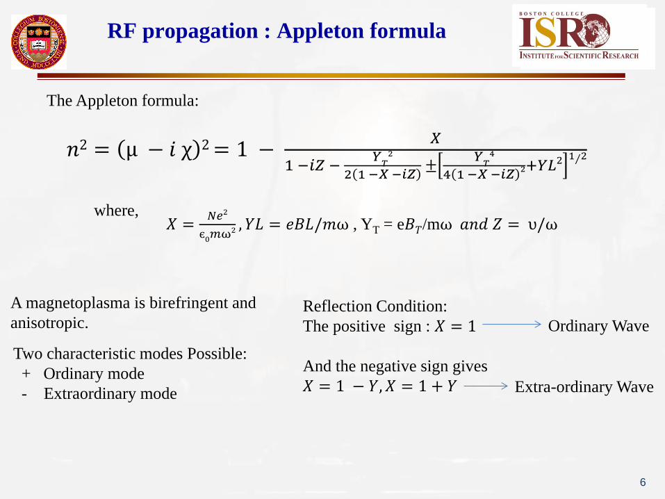
RF propagation : Appleton formula
𝑛2 = µ − 𝑖 χ 2 = 1 − 𝑋
1 −𝑖𝑍 − 𝑌𝑇2
2 1 −𝑋 −𝑖𝑍 ±
𝑌𝑇4
4 1 −𝑋 −𝑖𝑍 2+𝑌𝐿21 2
The Appleton formula:
𝑋 =𝑁𝑒2
є0𝑚ω2 , 𝑌𝐿 = 𝑒𝐵𝐿/𝑚ω , YT = e𝐵𝑇/mω 𝑎𝑛𝑑 𝑍 = υ/ω
where,
Two characteristic modes Possible:
+ Ordinary mode
- Extraordinary mode
A magnetoplasma is birefringent and
anisotropic. Reflection Condition:
The positive sign : 𝑋 = 1
And the negative sign gives
𝑋 = 1 − 𝑌, 𝑋 = 1 + 𝑌
Ordinary Wave
Extra-ordinary Wave
6

RF propagation : Appleton formula
α
α′
Higher Electron Density
Lower Electron Density Higher Refractive Index
Lower Refractive Index
α′ > α
Refraction of radio waves by the ionosphere due to the changes in
the electron density
When collisions are negligible :
𝑛2 = µ2 = 1 − 2𝑋(1 − 𝑋)
2(1 − 𝑋) − 𝑌𝑇2 ± 𝑌𝑇
2+ 4 1 − 𝑋 2𝑌𝐿2 1
2
When the magnetic field is negligible :
𝑛2 = µ − 𝑖 χ 2 = 1 −𝑋
1 − 𝑖𝑍
When both collisions and magnetic field effects are negligible :
𝑛2 = µ2 = 1 − X = 1 −𝑓𝑁
𝑓
2
• Cold Plasma
• No collisions
• No magnetic field
𝑓𝑁 = ; N is in electrons per cubic meter 9 𝑁
; 𝑓𝑁 = plasma frequency
7
= 𝜔
𝑝
2π =
𝑛𝑜𝑒2
ϵ0𝑚

Determination of Electron Densities
Ionosphere
T’ R’ T R
A
B
A’
B’
C
Earth
Oblique Vertical
Real Path
Virtual Path
T = Transmitter
R = Receiver
ℎ′ = 𝑐 𝑑ℎ
𝑢
ℎ𝑟
0 = 𝜇′𝑑ℎ
ℎ𝑟
0 Virtual Height :
8

Determination of Electron Densities
9
Incoherent Scatter Radar
Measures direct scatter from
electrons providing full height
density profile (f >> fpeak)
Ionosonde
Measures electron density profile up to the
peak density height only (f ≤ fpeak)

10
ALTAIR Radar
• Dual Frequency:
150 MHz/422 MHz
• Max Bandwidth:
7 MHz/18 MHz
• 46 m dish
• Peak Power
VHF: 6.0 MW
UHF: 6.4 MW
• Incoherent Scatter: Direct scatter from
electrons in the ionosphere (10-4 m2;
equivalent to a ~dime!)
Advanced Research Project Agency (ARPA)
Long-range Tracking and Identification
Radar (ALTAIR)

Transmitter/Receiver Geometry
Rongelap
Wotho
ALTAIR
Likiep
MOSC Release Location & Likiep-Wotho Mid-Point
11
• Rongelap-Wotho link geometry is predominantly N-S and great-circle path is far
from release region
• Likiep-Wotho path is nearly E-W and release point lies nearly on mid-point of
the link—should be ideal for observing SmO+ layer
N
E

12 12
Kwajalein Atoll

13 13
Roi Namur

14 14
THE RELEASE : MOVIE

15
CLOUD

Two Releases :
01 May and 09 May 2013
• Ionosphere during first release was disturbed, rising rapidly and Spread F formed within
minutes after release
• Ionosphere during second release is canonical quiescent
16

Rongelap TX Likiep TX
Mission 41102 09 May 2013 Pre-Release Sweep Wotho Receiver
• Sweeps from 2-30 MHz were completed every five (5) minutes - Plots show data from only
2-14 MHz since no signatures were observed at higher frequencies
• Slightly higher peak frequencies on Wotho Likiep path relative to Rongelap-Wotho links
probably due to longer path length, lower elevation angle propagation . 17
F -region
Ground Wave
F –region second hop

Rongelap TX Likiep TX
Mission 41102 09 May 2013 1st Post-Release Sweep Wotho Receiver
• On the Wotho geometry the layer extends up to 10 MHz peak frequency
• There is also a prominent secondary F region echo; the time delays will allow us to calculate
the range offsets
• The discrete nature of the echo suggests a localized perturbation that extends up to the F-
region peak
MOSC layer MOSC layer
F-layer Secondary Echo
18

Rongelap TX Likiep TX
Mission 41102 09 May 2013 2nd Post-Release Sweep Wotho Receiver
• The layer has now decreased to about 6 MHz peak density
• The F-region perturbation extends only mid-way up the density profile
• The delay is much greater on the Rongelap link geometry compared to the Wotho
geometry providing valuable information on the nature of the perturbation
MOSC layer MOSC layer
F-layer Secondary Echo
F-layer Secondary Echo
19

Rongelap TX Likiep TX
Mission 41100 01 May 2013 3rd Post-Release Sweep Wotho Receiver
• No clear signatures on Rongelap link
• A bottomside F-region perturbation remains on the Wotho-Likiep link, as well as
a possible MOSC layer signature around 4 MHz
F region perturbation
MOSC layer?
20
21
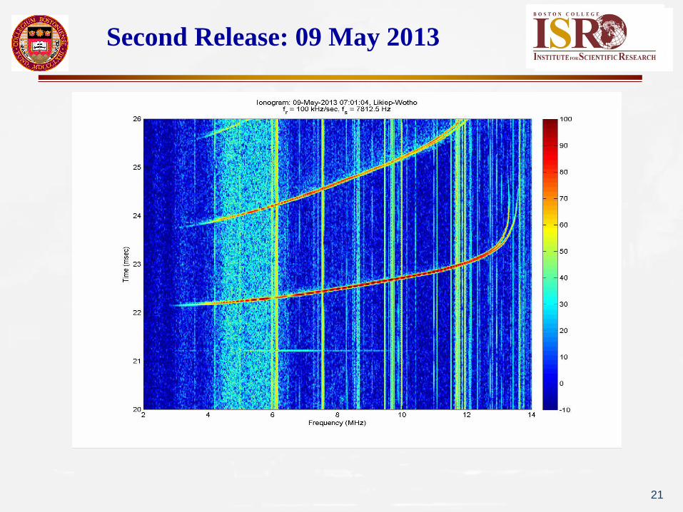
Second Release: 09 May 2013

22
Ionospheric Models
Goal : Model the Background Ionosphere and the Cloud
Background Ionosphere :
International Reference Ionosphere (IRI)
• Standard model of the empirical ionospheric
climatology
• Developed by joint working group of Committee on
Space Research (COSPAR) and International Union
of Radio Science (URSI)
• ‘Input variables’ : R12 , iono_layer_parms =
[foF2,hmF2,foF1,hmF1,foE,hmE]
Parametrized Ionospheric Model (PIM)
• Global model of theoretical ionospheric
climatology
• Combination of four physics-based numerical
ionospheric models
• ‘Input Variables’: F10.7 index, SSN, Kp index
Plots courtesy of William McNeil

23 23
IRI and ALTAIR Profiles
Approximately 30 seconds after release the MOSC
cloud has a peak density of about 106 e-/cc, slightly less
than the background ionosphere (Ne = 106 corresponds
to a plasma frequency of 9 MHz).
The layer is about 30 km in diameter by this time.
BEFORE
30 SEC AFTER

Time Period for
Modeling Cloud
MOSC Launch 2: May 9, 2013
Modeling the Cloud
24

25
The averaged and
symmetrized cloud
profile is used to
model the cloud in
MATLAB with
latitude/longitude
increment at
0.0141degree and
height increment at
1.5510 km . The
central pixel
corresponds to
7.4369 MHz
MOSC Launch 2: May 9, 2013
Modeling the Cloud

Ray Tracing
Haselgrove Equations:
• Fermat’s principle - δ 𝑚𝑑𝑠 = 0 , m is ray refractive index and ds the element of path length
• Variational method – ray path equations 𝑑𝑥𝑖𝑑𝑡
= 𝜕𝐺
𝜕𝑢𝑖
, 𝑑𝑢𝑖
𝑑𝑡 = -
𝜕𝐺
𝜕𝑥𝑖 ; 𝐺 = 𝑢 μ
• Numerical Integration of ray path equations : Runge Kutta method
Coleman Method :
• Point to point ray tracing
• Variational principle is discretized and resulting discretized equations solved
PHaRLAP:
• HF radio wave ray tracing toolbox developed by DSTO, Australia
• 2D raytracing is an implementation of the 2-D equations developed by Coleman
• 3-D engine is based upon the equations of Haselgrove
26

Ray Tracing : Example
27

• HF signals received well off the great
circle path to the receiver
• The artificial cloud bends the HF
energy through large angles
• Excellent agreement between model
and observations
Rongelap
Wotho
MOSC
Release
Point
3D Ray Trace Analysis
Rongelap To Wotho
28

• Great circle path to the receiver passes
through the MOSC volume
• Multiple paths between ionosphere, cloud
and receiver expected
Likiep
Wotho
MOSC Release Point
Likiep Wotho
MOSC
3D Ray Trace Analysis
Likiep To Wotho
29

Rongelap TX Likiep TX
Mission 41100 01 May 2013 Pre-Release Sweep Wotho Receiver
30
F -region
E - layer
Ground Wave
F-region – Second hop

Rongelap TX Likiep TX
Mission 41100 01 May 2013 1st Post-Release Sweep Wotho Receiver
• Note that the Likiep signature is only evident in high end of frequency range, showing up near f = 8 MHz
(~07:42 UT); one might conclude this is results from the temporal evolution of the cloud, yet the
Rongelap link shows the signature beginning at less than 4 MHz at least 40 seconds earlier.
• One possibility is that the lower frequency components on the direct Likiep-Wotho link were actually
blocked, refracted or ducted by the presence of the MOSC cloud.
MOSC layer MOSC layer
F-layer Secondary Echo
31

Rongelap TX Likiep TX
Mission 41100 01 May 2013 2nd Post-Release Sweep Wotho Receiver
• Peak density has decreased significantly over 5 minute time scale, primarily due to
expansion of the cloud
MOSC layer MOSC layer
32

Rongelap TX Likiep TX
Mission 41100 01 May 2013 3rd Post-Release Sweep Wotho Receiver
• The Rongelap path shows a low density residual signature of the cloud
• The Likiep path shows an emerging perturbation in the F-region
• By 07:56 and beyond MOSC has disappeared and Spread F dominates
MOSC layer F region perturbation
33

34
First Release: 01 May 2013

MOSC Launch 1: May 1, 2013
Modeling the Ionosphere
The ‘ALTAIR’ is modelled by applying the same relative differences as in PIM in lat-lon
plane at an altitude. The technique is applied at all altitudes. As is seen, modeled ‘ALTAIR’
fails to capture the shape of the high frequency tilt in PIM. 35
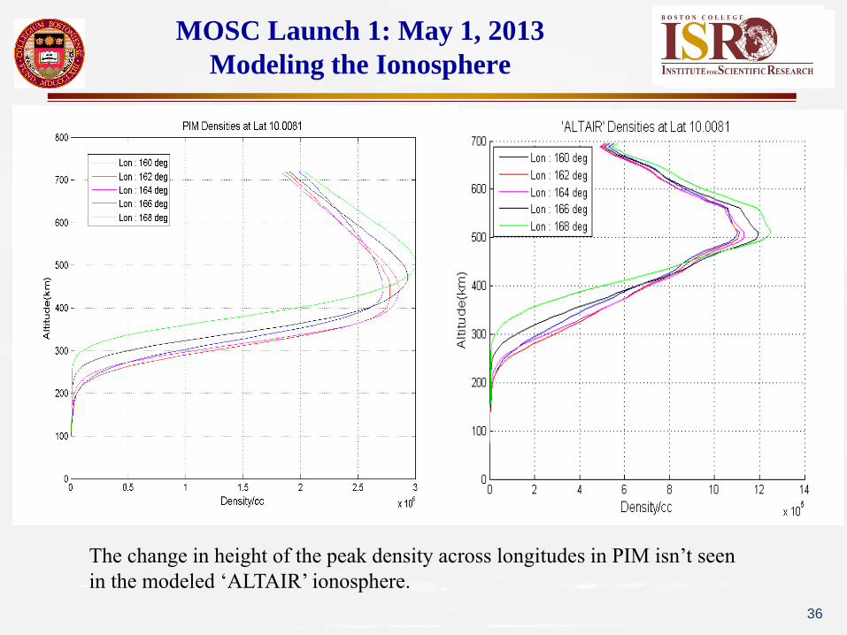
MOSC Launch 1: May 1, 2013
Modeling the Ionosphere
36
The change in height of the peak density across longitudes in PIM isn’t seen
in the modeled ‘ALTAIR’ ionosphere.

MOSC Launch 1: May 1, 2013
Modeling the Ionosphere
37
An averaged shape function is chosen to apply to the change in the height of the
peak density across longitudes.
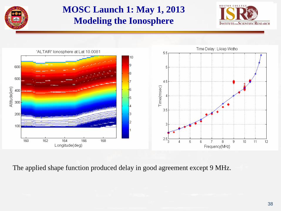
MOSC Launch 1: May 1, 2013
Modeling the Ionosphere
38
The applied shape function produced delay in good agreement except 9 MHz.

MOSC Launch 1: May 1, 2013
Modeling the Ionosphere
39
• The anchor profile is taken to be the
average of three ALTAIR radar profiles.
• This gives delay to a good agreement
with the observations.
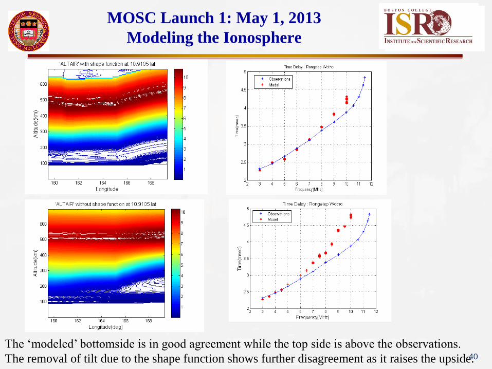
MOSC Launch 1: May 1, 2013
Modeling the Ionosphere
The ‘modeled’ bottomside is in good agreement while the top side is above the observations.
The removal of tilt due to the shape function shows further disagreement as it raises the upside. 40

Optimization : Nalder Mead Down Hill Simplex Method ( Amoeba)*
• Nelder, J. and R. Mead ,1965
• Direct Method : No derivatives, only function values
• Idea : Move from high function (hot) areas to low function
(cold) areas by reflections, expansions and contractions
• “Amoeba Crawls Downhill with no assumption about function”
• Built-in function in MATLAB : fminsearch
Modeling : Optimization Method
41 *Minimization Technique suggested by Dr. Charles Carrano, ISR

42
Optimization : Model Ionosphere
PIM doesn’t have enough degrees of freedom to fit the ALTAIR radar profile while
optimization of foF2 and hoF2 in IRI closely matches the observed ALTAIR radar
profile.
Scale Vector = [ a b c …. e]

43
Optimization : Delay results
The IRI model, scaled and unscaled, doesn’t match the observed delay.

Optimization : Delay results
44
• Optimization of the scaling vector matches only the upside
• Frequency specific optimization of the scale vector exactly reproduces the observed delay.
Conclusions
• Ray tracing confirms sounder observations to high degree of fidelity
• The change in ambient natural propagation environment due to small
artificial modification can be successfully modeled
• Effects from arbitrary artificial plasma environments can be predicted
with accuracy
• Optimization technique represents a new method of assimilating
oblique ionosonde data to generate the background ionosphere
(numerous applications for HF systems)
• Future Work : Modeling of natural disturbances in the low latitude
propagation environment to understand the effects of Traveling
Ionospheric Disturbances (TIDs) and Spread F on perpendicular and
quasi-parallel (to B) paths.
46

Thank You.
47


![[HF] FREEWEIGHT PRODUCTS - HOIST Fitness · [hf] flat bench hf-5163 [hf] 7-position folding f.i.d. bench hf-5167 new! warranty new! warranty [hf] 7-position f.i.d. olympic bench hf-5170](https://img.dokumen.tips/doc/110x75/5b5909d87f8b9ad0048c899a/hf-freeweight-products-hoist-fitness-hf-flat-bench-hf-5163-hf-7-position.jpg)