Height models on a honeycomb lattice - wiese.itp.unibe.ch · model, a two-dimensional lattice model on a honeycomb lattice, is deﬁned to have an integer-valued height variable (or

Height models on a honeycomb lattice

Masterarbeitder Philosophisch-naturwissenschaftlichen Fakultät

der Universität Bern

vorgelegt vonBühlmann Patrick

2018

Leiter der ArbeitProf. Dr. Uwe-Jens Wiese

Albert Einstein Center for Fundamental PhysicsInstitute for Theoretical Physics

University of Bern

Abstract

In this thesis we study a two-dimensional constrained height model on a honeycomb lattice, mo-tivated by a lecture given by Prof. M. Hairer in 2016 at the University of Bern. This model hasa one-to-one correspondence to an F Model on a triangular lattice. By using a multi-cluster algo-rithm, we simulate this model and obtain a dual form of a Berezinsky-Kosterlitz-Thouless phasetransition which is being investigated.

Contents

1 Introduction 1

2 Classical Statistical Mechanics 3

2.1 Partition Function . . . . . . . . . . . . . . . . . . . . . . . . . . . . . . . . . . . . . . . 32.2 Classical Spin Models . . . . . . . . . . . . . . . . . . . . . . . . . . . . . . . . . . . . . 3

2.2.1 Clock Model . . . . . . . . . . . . . . . . . . . . . . . . . . . . . . . . . . . . . . 32.2.2 U(1) Model and the XY Model . . . . . . . . . . . . . . . . . . . . . . . . . . . . 42.2.3 Height Model . . . . . . . . . . . . . . . . . . . . . . . . . . . . . . . . . . . . . 5

2.3 Dualization Relations among these Models . . . . . . . . . . . . . . . . . . . . . . . . . 52.3.1 Dualization of the Clock Model on a Square Lattice . . . . . . . . . . . . . . . . 52.3.2 Dualization of the XY Model . . . . . . . . . . . . . . . . . . . . . . . . . . . . . 8

2.4 F Model on a Triangular Lattice (F∆ Model) . . . . . . . . . . . . . . . . . . . . . . . . 102.5 Observables . . . . . . . . . . . . . . . . . . . . . . . . . . . . . . . . . . . . . . . . . . 102.6 Phase Transitions . . . . . . . . . . . . . . . . . . . . . . . . . . . . . . . . . . . . . . . 11

2.6.1 Disordered Phase and Ordered Phase . . . . . . . . . . . . . . . . . . . . . . . . 122.6.2 Spatial Correlations . . . . . . . . . . . . . . . . . . . . . . . . . . . . . . . . . . 122.6.3 Critical Exponents . . . . . . . . . . . . . . . . . . . . . . . . . . . . . . . . . . 132.6.4 Finite-Size Scaling . . . . . . . . . . . . . . . . . . . . . . . . . . . . . . . . . . . 132.6.5 Berezinsky-Kosterlitz-Thouless Phase Transition (BKT-transition) . . . . . . . 14

3 Monte Carlo Simulations 17

3.1 Markov Chains . . . . . . . . . . . . . . . . . . . . . . . . . . . . . . . . . . . . . . . . . 173.2 Measurements and Error Estimations . . . . . . . . . . . . . . . . . . . . . . . . . . . . 173.3 Autocorrelation . . . . . . . . . . . . . . . . . . . . . . . . . . . . . . . . . . . . . . . . 183.4 Detailed Balance and Ergodicity . . . . . . . . . . . . . . . . . . . . . . . . . . . . . . . 183.5 Algorithms . . . . . . . . . . . . . . . . . . . . . . . . . . . . . . . . . . . . . . . . . . . 19

3.5.1 Single Spin Flip Method (Metropolis Algorithm) . . . . . . . . . . . . . . . . . 193.5.2 Cluster Flip Method (Swendsen-Wang Cluster Algorithm) . . . . . . . . . . . . 20

4 The Honeycomb Lattice 21

4.1 Description and Properties . . . . . . . . . . . . . . . . . . . . . . . . . . . . . . . . . . 214.2 Duality Transformation and Star-Triangle Transformation . . . . . . . . . . . . . . . . 22

4.2.1 The Star-Triangle Transformation . . . . . . . . . . . . . . . . . . . . . . . . . . 224.2.2 Dual Transformation of the Honeycomb Lattice . . . . . . . . . . . . . . . . . . 23

4.3 Boundary Conditions . . . . . . . . . . . . . . . . . . . . . . . . . . . . . . . . . . . . . 244.3.1 The Torus . . . . . . . . . . . . . . . . . . . . . . . . . . . . . . . . . . . . . . . 25

5 The F∆ Model 27

5.1 Definition of the F∆ Model . . . . . . . . . . . . . . . . . . . . . . . . . . . . . . . . . . 275.2 Equivalence of the F∆ Model and the F∆ Model . . . . . . . . . . . . . . . . . . . . . . 275.3 Dual Transformation for the Honeycomb Lattice . . . . . . . . . . . . . . . . . . . . . 28

5.3.1 Step 1) . . . . . . . . . . . . . . . . . . . . . . . . . . . . . . . . . . . . . . . . . 285.3.2 Step 2) . . . . . . . . . . . . . . . . . . . . . . . . . . . . . . . . . . . . . . . . . 285.3.3 Step 3) . . . . . . . . . . . . . . . . . . . . . . . . . . . . . . . . . . . . . . . . . 285.3.4 Step 4) . . . . . . . . . . . . . . . . . . . . . . . . . . . . . . . . . . . . . . . . . 315.3.5 Step 5) . . . . . . . . . . . . . . . . . . . . . . . . . . . . . . . . . . . . . . . . . 31

i

Contents

6 Algorithm for the F∆ Model 33

6.1 The Modulo 4 Formulation of the F∆ Model . . . . . . . . . . . . . . . . . . . . . . . . 336.1.1 Constraint Cluster Rules at Coupling K = 0 . . . . . . . . . . . . . . . . . . . . 346.1.2 Boundary Updates . . . . . . . . . . . . . . . . . . . . . . . . . . . . . . . . . . 356.1.3 Next-nearest-neighbor Interaction . . . . . . . . . . . . . . . . . . . . . . . . . 36

6.2 Detailed Balance and Ergodicity . . . . . . . . . . . . . . . . . . . . . . . . . . . . . . . 366.3 The Modulo 4 Formulation and the Ising Model . . . . . . . . . . . . . . . . . . . . . . 376.4 Improved Estimators . . . . . . . . . . . . . . . . . . . . . . . . . . . . . . . . . . . . . 386.5 Autocorrelation Effects . . . . . . . . . . . . . . . . . . . . . . . . . . . . . . . . . . . . 396.6 Jackknife Method for the Binder Cumulant . . . . . . . . . . . . . . . . . . . . . . . . . 40

7 Results 41

7.1 Distribution of the Magnetization of both Sublattices . . . . . . . . . . . . . . . . . . . 417.2 Susceptibility and Magnetization per Spin . . . . . . . . . . . . . . . . . . . . . . . . . 427.3 Correlation Function . . . . . . . . . . . . . . . . . . . . . . . . . . . . . . . . . . . . . 447.4 Binder Cumulant . . . . . . . . . . . . . . . . . . . . . . . . . . . . . . . . . . . . . . . 457.5 Finite-Size Scaling Procedure . . . . . . . . . . . . . . . . . . . . . . . . . . . . . . . . 467.6 Taylor Fit . . . . . . . . . . . . . . . . . . . . . . . . . . . . . . . . . . . . . . . . . . . . 487.7 Helicity Modulus . . . . . . . . . . . . . . . . . . . . . . . . . . . . . . . . . . . . . . . 49

8 Summary and Interpretation of the Results 51

9 Conclusion and Outlook 53

Acknowledgement 55

A Formulas 57

A.1 Fourier Representation . . . . . . . . . . . . . . . . . . . . . . . . . . . . . . . . . . . . 57A.2 Dirac Comb . . . . . . . . . . . . . . . . . . . . . . . . . . . . . . . . . . . . . . . . . . 57A.3 Poisson Summation Formula . . . . . . . . . . . . . . . . . . . . . . . . . . . . . . . . . 57

Selbstständigkeitserklärung 61

ii

1 Introduction

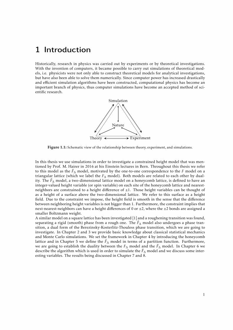
Historically, research in physics was carried out by experiments or by theoretical investigations.With the invention of computers, it became possible to carry out simulations of theoretical mod-els, i.e. physicists were not only able to construct theoretical models for analytical investigations,but have also been able to solve them numerically. Since computer power has increased drasticallyand efficient simulation algorithms have been constructed, computational physics has become animportant branch of physics, thus computer simulations have become an accepted method of sci-entific research.

Nature

Theory Experiment

Simulation

Figure 1.1: Schematic view of the relationship between theory, experiment, and simulations.

In this thesis we use simulations in order to investigate a constrained height model that was men-tioned by Prof. M. Hairer in 2016 at his Einstein lectures in Bern. Throughout this thesis we referto this model as the F∆ model, motivated by the one-to-one correspondence to the F model on atriangular lattice (which we label the F∆ model). Both models are related to each other by dual-ity. The F∆ model, a two-dimensional lattice model on a honeycomb lattice, is defined to have aninteger-valued height variable (or spin variable) on each site of the honeycomb lattice and nearest-neighbors are constrained to a height difference of ±1. Those height variables can be thought ofas a height of a surface above the two-dimensional lattice. We refer to this surface as a heightfield. Due to the constraint we impose, the height field is smooth in the sense that the differencebetween neighboring height variables is not bigger than 1. Furthermore, the constraint implies thatnext-nearest-neighbors can have a height differences of 0 or ±2, where the ±2 bonds are assigned asmaller Boltzmann weight.A similar model on a square lattice has been investigated [1] and a roughening transition was found,separating a rigid (smooth) phase from a rough one. The F∆ model also undergoes a phase tran-sition, a dual form of the Berezinsky-Kosterlitz-Thouless phase transition, which we are going toinvestigate. In Chapter 2 and 3 we provide basic knowledge about classical statistical mechanicsand Monte Carlo simulations. We set the framework in Chapter 4 by introducing the honeycomblattice and in Chapter 5 we define the F∆ model in terms of a partition function. Furthermore,we are going to establish the duality between the F∆ model and the F∆ model. In Chapter 6 wedescribe the algorithm which is used in order to simulate the F∆ model and we discuss some inter-esting variables. The results being discussed in Chapter 7 and 8.

1

2 Classical Statistical Mechanics

In this section basic features of classical statistical mechanics, with a focus on spin systems arebeing reviewed. The interested reader is referred to [2, 3] for a more detailed discussion.

2.1 Partition Function

Statistical mechanics is based upon the idea of a partition function which describes the statisti-cal properties of a system in thermodynamical equilibrium. For a classical statistical system thecanonical partition function is given by

Z(β) =∑[s]

e−βH[s], (2.1)

where H[s] is the Hamiltonian as a functional of a given spin configuration [s] and β = 1kBT

. Thevariable T denotes the temperature, kB is the Boltzmann constant, and the summation extends overall possible spin configurations. One defines observables as

〈O〉 =∑[s]

p[s]O[s], (2.2)

where O[s] denotes the measured quantity of the configuration [s] and p[s] denotes the probabilityof the system to be in a particular configuration [s] given by

p[s] =1

Z(β)e−βH[s]. (2.3)

2.2 Classical Spin Models

One distinguishes continuous and discrete spin models, depending on whether the spins take theirvalues in a continuous or discrete target space. Spin models can also be characterized by their latticegeometry and their dimensionality d. Throughout this thesis we only consider the two-dimensionalcase d = 2. Usually, when defining Hamiltonians of spin systems one adds a contribution in formof an external magnetic field h. In this thesis, however, we define all Hamiltonians in the absenceof symmetry breaking external fields. In 1952 Potts described a class of spin models [4] which arenamed after him, the standard q-state Potts model and the q-state clock model (which is also re-ferred to as a Zq-model or q-state planar Potts model).Both models impose a nearest-neighbor interaction and respect a q-periodicity (q ∈ N) such thateach spin variable can be parametrized by an integer-valued variable n ∈ {0,1, · · · ,q − 1}. The Boltz-mann weight u(nx,ny) for nearest-neighboring spins is a function of the difference only and it isperiodic with period q, such that

u(nx,ny) = u(ny −nx) = u(ny −nx mod q). (2.4)

For our discussion the q-state clock model is of particular interest.

2.2.1 Clock Model

For the q-state clock model one attaches a 2-component unit-vector to each lattice site x, such that

~ex = (cos(ϕx),sin(ϕx)). (2.5)

3

CHAPTER 2. CLASSICAL STATISTICAL MECHANICS

This unit-vector at lattice site x is parametrized by a discretized angle

ϕx =2πnxq

,nx ∈ {0,1, · · · ,q − 1}, (2.6)

such that the vector is pointing towards the corners of a planar q-gon. The q-state clock model ischaracterized by the energy function

Hclock[ϕ] = −J∑〈x,y〉

~ex.~ey = −J∑〈x,y〉

cos(ϕy −ϕx), (2.7)

where 〈x,y〉 indicates a summation over nearest-neighbors. Hence the partition function reads

Zclock(β) =∑[ϕ]

e−βHclock[ϕ] =

∏x

∑ϕx∈ 2π

q ·Zq

e−βHclock[ϕ] =

∏x

q−1∑nx=0

e−βHclock[ϕ]. (2.8)

Since the interaction only depends on spin differences it is invariant under globalZq-transformations

ϕx 7→ ϕx +2πnq,n ∈ Z,∀x. (2.9)

For the case where q = 2 the energy of a single bond is ±J , depending on whether the adjacentspins have the same value or not. Thus the case where q = 2 and J > 0 is equivalent to an Isingferromagnet, if we consider integer-valued spins sx ∈ {±1} and modify the Hamiltonian

HIsing[s] = −J∑〈x,y〉

sxsy . (2.10)

We are going to use the Ising ferromagnet as a prime example throughout this thesis, in order toillustrate certain theoretical concepts.

2.2.2 U(1) Model and the XY Model

The U (1) model can be obtained from the q-state clock model in the limit of infinite q. In this limitthe angles ϕx can take any value between 0 and 2π, such that a spin is parametrized by an angle ona unit circle S1. As the name suggests, this model has a global U (1) symmetry, which means thatthe Hamiltonian stays invariant under a global angular valued transformation by a fixed angle ϕ

ϕx 7→ ϕx + ϕ, ϕ ∈ [0,2π),∀x. (2.11)

The two-dimensional U (1) model, which is known as the XY model, shows an unusual phase tran-sition of infinite order, which is known as a Berezinsky-Kosterlitz-Thouless phase transition (seeSubsection 2.6.5). In order to define the XY model, consider a two-dimensional lattice where eachsite carries a unit-vector as in Equation (2.5), parametrized by a continuous angle ϕ ∈ [0,2π). An-gular differences are defined to be

∆ϕxy = ϕy −ϕx mod 2π, ∆ϕxy ∈ [0,2π), (2.12)

and the Hamiltonian is the same as for the q-state clock model

HXY[ϕ] = −J∑〈x,y〉

cos(ϕy −ϕx). (2.13)

Since configurations [ϕ] are now described by continuous angular variables the summation in thepartition function of the clock model is now replaced by an integration. Therefore we obtain forthe XY model

ZXY(β) =(∫Dϕ

)e−βHXY[ϕ] =

∏x

∫ 2π

0dϕx

e−βHXY[ϕ]. (2.14)

4

2.3. DUALIZATION RELATIONS AMONG THESE MODELS

2.2.3 Height Model

Consider a spin model where each lattice site x is inhabited by an integer-valued spin variablehx ∈ Z. In this case the spins are interpreted as height variables. The difference of heights hy − hxfor adjacent lattice points x and y is related to the Hamiltonian H[h]. Consider for example theHamiltonian

H[h] =J4

∑〈x,y〉

(hy − hx)2, (2.15)

where J > 0 and we have integer-valued height variables hx ∈ Z. We see that in the limit wherethe temperature T goes to 0, flat height fields have a higher Boltzmann weight, whereas for hightemperatures fluctuating height fields are more dominant in the partition function. Throughoutthis thesis, flat height fields, where fluctuations between neighboring height variables are mini-mized, are considered smooth height fields. They are characteristic for the rigid (smooth) phase,whereas fluctuating height fields are characteristic for the rough phase. Allowing the heights tobe integer-valued is problematic because the partition function is not well-defined anymore. AnyHamiltonian depending on height differences is invariant under global shifts hx 7→ hx + n, for anyn ∈ Z, which means that we have an infinite number of configurations. One can get rid of the globalZ symmetry by fixing one height variable and imposing constraints which only allow for a finitenumber of configurations.

2.3 Dualization Relations among these Models

The previously presented lattice models are related to each other by duality transformations. Adiscussion of duality transformations and their geometrical interpretation for the honeycomb lat-tice is given in Chapter 4, and a detailed transformation for the F∆ model is given in Chapter 5.A duality transformation maps a system of low temperature to a system of high temperature (andvice versa) and leads to new insights into critical regimes of the model. For a simple case like theIsing model, one can also say that an ordered phase (at low temperature) is mapped to a disorderedphase (at high temperature) and vice versa. In the case where two lattice models are identical up toa rescaling of the Boltzmann weights we call a model self-dual. The dual transformation was firstintroduced for the Ising model on a square lattice by Kramers and Wannier in 1941 [5], in 1945 thedual lattice was introduced by Wannier giving a topological picture of the dual transformation [6].Throughout this thesis the variables x,y denote coordinates of the original lattice and variableswith a tilde like x, y denote coordinates of the dual lattice.

2.3.1 Dualization of the Clock Model on a Square Lattice

Consider the zero field q-state clock model on a square lattice, with Hamiltonian Hclock[ϕ], givenin Equation (2.7). The Boltzmann weights factorize such that the partition function can be writtenas

Z(β) =∑[ϕ]

e−βH[ϕ] =∑[ϕ]

∏〈x,y〉

u(ny −nx). (2.16)

where u(ny − nx) is the q-periodic Boltzmann factor. For the sake of simplicity we introduce adimensionless coupling parameter

K = βJ, (2.17)

such that the partition function Z is a function of K (Z = Z(K)) and

u(ny −nx) = eK cos( 2πq (ny−nx)). (2.18)

5


We assume that the square lattice hasN sites and we impose open boundary conditions. In order todualize this model we need to impose an orientation on the bonds of the square lattice, indicatinghow we measure spin differences. We determine spin differences by the sense of arrows pointingup and right (see Figure 2.1). Duality of the partition function is derived by using the Fourier

xx+ xx − x

x+ y

x − y

Figure 2.1: Definition of spin differ-ences determined by thesense of arrows. The unit-vectors along the x and yaxes are labeled x and y.

xx+ xx − x

x+ y

x − y

xx − x

x − x− y x − y

Figure 2.2: New spin variables nx intro-duced on the dual lattice. Coor-dinates of the dual lattice are de-noted by a tilde, such as x.

transformation of the Boltzmann factor at each bond, such that

u(ny −nx) =1q

q−1∑kxy=0

exp(

2πiq

(ny −nx)kxy

)λ(kxy). (2.19)

Now the dependence on nx is very simple and we can evaluate the partition function for this case.Plugging in Equation (2.19) we obtain

Z(K) =∑[ϕ]

∏〈x,y〉

u(ny −nx) =∑[ϕ]

∏〈x,y〉

1q

q−1∑kxy=0

e2πiq (ny−nx)kxyλ(kxy)

(2.20)

= (1q

)2N

∏〈x,y〉

q−1∑kxy=0

λ(kxy)

∏x

q−1∑nx=0

∏〈x,y〉

e2πiq (ny−nx)kxy

. (2.21)

The case of the square lattice implies that for a given x, the variable nx appears in the Boltzmannfactor for interactions with four neighboring sites. According to the way we defined spin differ-ences, with the sense of arrows as up and right, we assign the sign such that x is at the head of anarrow and y is the tail in nx −ny . Then the summation over one site x is of the form

q−1∑nx=0

exp(

2πiq

((nx+x −nx)kx,x+x + (nx −nx−x)kx−x,x + (nx+y −nx)kx,x+y + (nx −nx−y)kx−y,x

)). (2.22)

Evaluating the sum over nx yields the constraint

kx,x+x − kx−x,x + kx,x+y − kx−y,x mod q = 0, (2.23)

for all lattice sites. The variables kxy act as bond variables between the spins. If we consider kxy as acurrent flowing along the bond 〈x,y〉, Equation (2.23) suggests that the current is conserved at each

6


site and thus the field is free of divergence. The partition function then takes the form

Z(K) = qN−2N∗∑

[kxy ]

∏〈x,y〉

λ(kxy), (2.24)

where∑∗

[kxy ] denotes the sum over all bond configurations satisfying the constraint. The factor q−2N

is a result of the 2N bonds and the definition of the discrete Fourier transformation. Assuming thatall constraints are satisfied, the factor qN comes out after summing over all bond variables kxy . Thenext step is to find a change of variables such that the constraints are satisfied. These variablesare considered dual variables living on the dual lattice (see Figure 2.2). We first rotate the originalbonds kxy consistently by an angle of 90 degrees and impose new variables n at the tail of the arrowsand at the head of the arrows. Define the new variables to be

kx,x+x = nx − nx−y, kx,x+y = nx−x − nx, (2.25)

kx−x,x = nx−x − nx−x−y, kx−y,x = nx−x−y − nx−y, (2.26)

all of which are modulo q, and we introduced dual coordinates x on the dual lattice. Using thischange of variables the constraint is satisfied and we end up with the dual partition function givenby

Z(K) =(

1q

)N ∑[n]

∏〈x,y〉

λ(ny − nx) = (1q

)N Z(K), (2.27)

where K denotes the dual partition function with some dual coupling parameter K . The Boltzmannweight λ for the dual partition function Z reads

λ(ny − nx) =q−1∑kxy=0

exp(−2πiq

(ny − nx)kxy

)u(kxy)

=q−1∑kxy=0

exp(−i(

2πnyq− 2πnx

q)kxy +K cos(

2πkxyq

)). (2.28)

The dual Boltzmann weight λ is q-periodic, has its maximum at λ(0) and its minimum at λ(q/2) forq even or λ((q+1)/2),λ((q−1)/2) for q odd. These are the same characteristics the original Boltzmannweight u has, therefore λ describes the same physics and the model is self-dual. Ideally we want torelate the dual Boltzmann weight λ = λ(ny − nx), with its dual coupling parameter K such that

λ(ny − nx) ∝ eK cos( 2πq (ny−nx)). (2.29)

Using this identification one tries to deduce a duality relation between K and K such that we canassociate a weak coupling phase in K with a strong coupling phase in K and vice versa. For gen-eral q such a relation is difficult to deduce analytically, but for the case q = 2 (Ising model) it canbe accomplished. For q = 2 we have u(0) = eK , u(1) = e−K in the original model. The Boltzmannweights of the dual model then read λ(0) = eK + e−K and λ(1) = eK − e−K . Since the ratio of Boltz-mann factors for the two states of neighboring spins is u(1)/u(0) = e−2K , it is reasonable to defineλ(1)/λ(0) = e−2K , such that the duality between the two couplings reads

e−2K = tanh(K)↔ (e2K − 1)(e2K − 1) = 2. (2.30)

The dual Boltzmann weight λ is now given by

λ(ny − nx) = eK cos(π(ny−nx))+a, (2.31)

7


where the constant a comes from the ambiguity of the multiplicative factor in λ(1)/λ(0). Usingλ(0) = eK + e−K = eK+a, we can fix this constant such that in the very end the partition functionreads

Z(K) =(1

2

)NZ(K) =

(12

)N (2cosh(K)

eK

)2N

Z(K). (2.32)

From this dual relation we can see that if K → 0, we have K →∞, which means that a disorderedphase in the original model (at high temperature) is mapped to an ordered phase in the dual model(and vice versa). The duality relation in Equation (2.30) allows us to analytically determine thecritical coupling Kc, where the second order phase transition for the Ising model takes place. Thetransition takes place when K = K = Kc, so we can solve Equation (2.30) for Kc and obtain

Kc =ln(1 +

√2)

2. (2.33)

The geometrical interpretation of a dual transformation uses the idea of a dual lattice, where thedual model lives. The dual lattice of an arbitrary lattice is constructed by putting a lattice point(designated by a cross) in the interior of every elementary polygon of the original lattice and con-necting them by a new dual interaction bond (dashed lines). In Figure 2.3 and 2.4 we see that the

Figure 2.3: Dual lattice of square lat-tice.

Figure 2.4: Dual lattice of the honeycomblattice.

square lattice is self-dual (in the sense that its dual is also a square lattice) and the dual lattice ofthe honeycomb lattice is a triangular lattice. Since the duality relation is reciprocal, the dual of thetriangular lattice is again a honeycomb lattice. If we want to obtain a duality relation for a spinmodel on a honeycomb lattice, we need to consider an additional transformation, which is knownas the star-triangle-transformation (see Chapter 4).

2.3.2 Dualization of the XY Model

We showed that the q-state planar clock model on the square lattice is self-dual. Here we want toshow that an XY model is mapped to a two-dimensional height model by a duality transformation.Consider an XY model on a square lattice with partition function

ZXY(K) =(∫Dϕ

)∏〈x,y〉

u(ϕy −ϕx) =(∫Dϕ

)∏〈x,y〉

eK cos(ϕy−ϕx), (2.34)

where we introduced once again the dimensionless coupling parameter K = βJ and implicitly gavea definition for the Boltzmann weight u(ϕy −ϕx). In order to perform the dual transformation weuse the Fourier expansion such that

u(ϕy −ϕx) =∑kxy∈Z

eikxy (ϕy−ϕx)λ(kxy). (2.35)

8


Applying the same procedure as in Subsection 2.3.1 yields that

ZXY(K) ∝ ZH.M.(K), (2.36)

where ZH.M(K) is given by

ZH.M.(K) =∑[h]

∏〈x,y〉

λ(|hx − hy |). (2.37)

In the previous expression [h] denotes an integer-valued height configuration on the dual lattice,and λ(|hx − hy |) is the modified Bessel function given by

λ(|hx − hy |) =1

2π

∫ 2π

0eK cos(ϕ)e−i|hx−hy |ϕdϕ

=1

2π

∫ 2π

0eK cos(ϕ) cos(|hx − hy |ϕ)dϕ. (2.38)

From the dualization procedure we can see that we turn the angular-valued XY model into a heightmodel, where the degrees of freedom are integer-valued height variables. This transformation doesnot yield an algebraic relation between the coupling parameter K and the dual coupling parameterK , like we had for the q = 2 clock model. In order to obtain such a relation we modify the originalXY model by applying a Villain-style replacement [7–9],

u(ϕ) = eK cos(ϕ) 7→ w(ϕ) =∑p∈Z

e−K2 (ϕ−2πp)2

, (2.39)

where w(ϕ) is a 2π-periodic function that is peaked at ϕ = 0, like the original XY Boltzmann weightu(ϕ). Thus the physics is qualitatively the same. By using the Poisson summation formula (seeappendix A.3), we obtain

w(ϕ) =∑p∈Z

e−K2 (ϕ−2πp)2

=1

√2πK

∑n∈Z

einϕ−1

2K n2. (2.40)

The partition function can then be written as

ZXY(K) =(∫Dϕ

)∏〈x,y〉

w(ϕy −ϕx)

∝(∫Dϕ

)∏〈x,y〉

∑nxy∈Z

einxy (ϕy−ϕx)− 12K n

2xy . (2.41)

Evaluating the integrals over the angles ϕx yields the vanishing of the lattice divergence, we havealready encountered in Subsection 2.3.1, such that

ZH.M.(K) ∝∗∑

[nxy ]

∏〈x,y〉

e−K2 n

2xy . (2.42)

Once again∑∗

[nxy ] denotes a summation over all bond configurations which satisfy the constraint

and we defined the dual coupling parameter K = 1/K . The vanishing lattice divergence enablesus to write nxy in terms of integer-valued height variables [h] living on the dual lattice, such thatnxy = hy − hx. The vanishing lattice divergence guarantees that the integer heights are definedconsistently up to an unimportant overall shift. The constrained partition function can then bewritten as an unconstrained sum over all integer-valued heights

ZH.M.(K) ∝∑[h]

∏〈x,y〉

e−K2 (hx−hy )2

. (2.43)

9


The duality relation among the coupling variables

KK = 1, (2.44)

shows that the strong coupling phase of the XY model (large value of K) belongs to a weak couplingphase of the height model (small value of K).

2.4 F Model on a Triangular Lattice (F∆ Model)

The F∆ model we are going to investigate is equivalent to the so-called F model on a triangularlattice [10], which is a constrained 20-vertex model. Here we give a quick introduction for theF∆ model, the equivalence is shown in Section 5.2. Suppose that arrows are placed on bonds of atriangular lattice, such that there are three arrows entering and three arrows leaving each vertex.There exist 20 different configurations of arrows at each vertex. If we identify configurations withall arrows reversed we obtain the 10 distinct configurations shown in Figure 2.5.

1 2 3 4 5

6 7 8 9 10

Figure 2.5: Ten distinct reversal-symmetric vertex configurations

This is the original 20-vertex model, where we could assign different weights to each of these ver-tices. The F∆ model identifies configurations which are related to each other by rotation and reflec-tion and gives them the same weight. The different vertices are classified as follows

1. 2 vertices, in which ingoing and outgoing arrows are adjacent (vertex 1).

2. 12 vertices, where two incoming arrows are adjacent and the third arrow enters in the oppo-site way (vertex 2,3,4,5,6,7).

3. 6 vertices, in which the three incoming arrows are adjacent (vertex 8,9,10).

Now we assign energies ε0,ε1,ε2 to each of these types of vertices. The first type has energy ε0,which is the ground state energy, the second type has energy ε1, the third one energy ε2, such thatε0 < ε1 < ε2. The corresponding Boltzmann weights are given by wi = exp(−βεi). The F∆ modelwas solved analytically by Baxter [10], under the subsidiary condition that the Boltzmann weightssatisfy

(w2 −w1)2 = w2(w0 −w1). (2.45)

2.5 Observables

In order to study a statistical model, we are interested in various observables, which provide uswith information about macroscopic properties of the system. Interesting observables for the Isingferromagnetic are, for instance, the thermal expectation value of the energy 〈H〉 and the magneti-zation 〈M〉. The internal energy and the magnetization for a specific configuration [s] are defined

10

2.6. PHASE TRANSITIONS

as

HIsing[s] = −J∑〈x,y〉

sxsy (2.46)

and

M[s] =∑x

sx. (2.47)

The internal energy 〈H〉 is then given by

〈H〉 =∑[s]

H[s]p[s] =1

Z(β)

∑[s]

H[s]e−βH[s]. (2.48)

Using the specific heat

CV =∂〈H(T )〉∂T

∣∣∣∣∣V

(2.49)

and the relation

−∂〈H(β)〉∂β

∣∣∣∣∣V

= 〈H2〉 − 〈H〉2, (2.50)

one can derive a fluctuation relation for the energy of the macroscopic system

CV kBT2 = 〈H2〉 − 〈H〉2 = 〈(∆H)2〉. (2.51)

Similar fluctuation relations also hold for other quantities, e.g., for the isothermal susceptibility

χ =∂〈M〉∂H

∣∣∣∣∣T, (2.52)

such that one obtainskBT χ = 〈M2〉 − 〈M〉2. (2.53)

For height models there are other interesting quantities namely the winding numbers Wx and Wy ,which characterize the boundary conditions. The free energy of a system describes quantitativelythe capacity of a system to perform work and can be determined from the partition function

F(β) = −kBT log(Z(β)). (2.54)

Thermodynamic quantities can be calculated by appropriate differentiation of the free energy e.g.

〈H〉 = −T 2∂(F(β))T )∂T

, 〈M〉 = −∂F(β)∂H

. (2.55)

2.6 Phase Transitions

The term phase transition is most commonly used in order to describe transitions between solid,gaseous, and liquid states of matter. A thermodynamical system in a phase has uniform physicalproperties, which change continuously as a function of some external parameters, such as temper-ature, pressure or even both. In this chapter we assume this parameter to be the temperature T .At a certain critical temperature Tc the statistical system undergoes a phase transition, where cer-tain properties change, often discontinuously. A first order phase transition is characterized by thefact that the first derivative of the free energy with respect to T is discontinuous at the transitiontemperature. For a second order phase transition the first derivative is continuous, but the secondderivative at the critical temperature Tc is characterized by a singularity. Since phase transitionsand phase diagrams are difficult to compute analytically, we need simulations in order to describethem quantitatively. The discussion on phase transitions in this subsection is limited to classicalstatistical mechanics.

11


2.6.1 Disordered Phase and Ordered Phase

The Ising ferromagnet has a second order phase transition, which can be characterized using themagnetization 〈M〉 as an order parameter. In the disordered phase (T > Tc), adjacent spins of aconfiguration [s] tend to align themselves independently of each other, such that the overall mag-netization of a spin configuration is close to zero (M[s] ≈ 0). Below the phase transition (T < Tc)multiple different ordered states may appear since they are energetically favorable and adjacentspins tend to align in the same direction. The critical temperature can be estimated by consideringthe behavior of the order parameterM as a function of T . Using the theoretical pictureM(T ) (seeFigure 2.6) we can distinguish the ordered phase (T < Tc) from the disordered phase (T > Tc).

Figure 2.6: MagnetizationM per spin as a function of T (Ising model).

Note that for a system with short-range interactions and dimension d ≤ 2, the Mermin-Wagnertheorem states that continuous symmetries cannot be spontaneously broken at finite tempera-ture [11, 12]. Since U (1) models have a continuous U (1) symmetry, the theorem implies that wecan not have a completely ordered phase because long-range fluctuations can be created with asmall amount of energy. Therefore the simple picture which works for the Ising model needs to bemodified for a two-dimensional U (1) model (see Subsection 2.6.5).

2.6.2 Spatial Correlations

Even if a system is not ordered, in general there exist regions in which the characteristics of thematerial are correlated. Since we are interested in spin models, we want to measure regions wherespins are spatially correlated. The spatial correlation for an Ising ferromagnet can be measuredthrough a 2-point function

Γ (r) = 〈s0sr〉 − 〈s0〉〈sr〉, (2.56)

where r is the distance between the spin variables. In the limit where r goes to infinity the 2-pointcorrelation function has the form

Γ (r) ∝ 1rηe−

rξ , (2.57)

where η is a critical exponent and ξ = ξ(T ) is the so-called correlation length, which is a measure forthe size of a region in which the Ising spins are correlated. In the disordered phase the correlationlength is typically just a few lattice spacings but at the critical temperature Tc, the correlation lengthdiverges with a critical exponent ν such that

limT→Tc

ξ ∝ |T − Tc |−ν . (2.58)

In the ordered phase the correlation length is infinite and the correlation function approaches aconstant value.

12


2.6.3 Critical Exponents

Thermodynamical properties of a statistical system can be described by a set of simple power lawsin the vicinity of the critical point T = Tc.The Ising ferromagnet has the order parameter 〈M〉, the specific heat CV , the susceptibility χ, butalso the spatial correlation function Γ , which have a power law behavior near the critical point. Inthe vicinity of the critical point these are given by

〈M〉 ∝ |T − Tc |β ,T ≤ Tc, χ ∝ |T − Tc |−γ ,CV ∝ |T − Tc |−α , ξ ∝ |T − Tc |−ν , (2.59)

Γ (r) ∝ 1rη, r→∞.

To summarize, we have introduced five critical exponents α,β,γ,ν, and η. In the specific case ofthe two-dimensional Ising ferromagnetic these take the values

α = 0, β =18, γ =

74, ν = 1, η =

14. (2.60)

Critical exponents are known analytically only for a certain number of statistical systems, but theyare very helpful in order to classify statistical systems into universality classes, where all models ofthe same class share the same critical behavior.

2.6.4 Finite-Size Scaling

When performing numerical simulations on a lattice, the critical behavior of a system can be ex-tracted from the size-dependence of the free energy and other observables near the critical point.According to the finite-size scaling theory (see Fisher [13], Privman [14], or Binder [15]) a scalingansatz can be written as

F(L,T ) = L−2−αν F (εL

1ν ), (2.61)

where F is some scaling function, L describes the lattice size and ε = |T −Tc |. It is important to noticethat the critical exponents are defined in infinite lattice volumes. The choice of the scaling variablez = εL

1ν is motivated by the fact that the correlation length ξ ∝ ε−ν , for T → Tc, is limited by the

lattice size L, which implies that Lξ ∝ ε

νL, is finite and we might as well take z = εL1ν . Appropriate

differentiation on the free energy yield the following scaling forms

M = L−βνM0(εL

1ν ),

χ = Lγν χ0(εL

1ν ), (2.62)

CV = Lαν C0

V (εL1ν ).

These relations have been derived with the help of the following scaling relations

(2− η)ν = γ,ν2

(η + d − 2) = β, (2.63)

2− νd = α,

and by using certain substitutions in Equation (2.61). The scaling forms (2.62) and the scalingrelations in Equation (2.63) are valid only for sufficiently large L and at temperatures close to Tc.Exactly at the transition point we have z→ 0, and the scaling functions,M0(0),χ0(0), and C0

V (0),reduce to proportionality constants, such that we obtain

M∝ L−βν ,

χ ∝ Lγν , (2.64)

CV ∝ Lαν , at T = Tc.

13


Note that the scaling functions in (2.62) are universal, apart from the scale factors for their argu-ments. Since we described the critical behavior of the statistical system, one also needs to explainhow to obtain the critical point in the first place. By examining higher-order moments of the mag-netization, Binder described a procedure how to derive the critical point of a statistical system [16].For an Ising model, the Binder cumulant is defined as

U4 = 1− 〈M4〉

3〈M2〉2, (2.65)

such that in the case where the lattice size goes to infinity U4 → 0 for T > Tc and U4 → 2/3 forT < Tc. For different lattice sizes, curves of U4 cross as a function of the temperature at the fixedpoint T = Tc and at a certain value U ∗. Hence by making plots for different lattice sizes one gets afirst estimate for Tc, from the location of the crossing point. The crossing points for different latticesizes are going to vary, but nonetheless there should be a general trend towards a fixed critical pointTc. Throughout this thesis instead of the original Binder cumulant given in Equation (2.65) we aregoing to use

U4 =〈M4〉〈M2〉2

, (2.66)

which satisfies the same purpose.

2.6.5 Berezinsky-Kosterlitz-Thouless Phase Transition (BKT-transition)

In 2016 the physics Nobel prize was given to John Kosterlitz and David Thouless based on theirworks on phase transitions of infinite order. A BKT-transition is therefore characterized by the factthat the free energy is an infinitely differentiable function, which makes the transition itself verysmooth. This kind of phase transition was extensively investigated in the classical XY model (seeSubsection 2.2.2).For a system with short-range interactions and dimension d ≤ 2, the Mermin-Wagner theorem statesthat continuous symmetries cannot be spontaneously broken at finite temperatures [11, 12]. Sincethe XY model has a U (1) symmetry, the theorem implies that we can not have a completely orderedphase because long-range fluctuations can be created with little energy. Hence the Ising ferromag-net, which has a discrete Z2 symmetry is allowed to have an ordered phase for T < Tc, whereas theclassical XY model for T < Tc has a quasi-ordered superfluid phase instead [7]. We conclude thatthe XY model has two phases, a superfluid phase for T < Tc and a disordered phase for T > Tc. Atthe critical temperature Tc the BKT-transition takes place. The disordered phase is characterizedby a short-range correlation with a finite correlation length ξ <∞ such that

Γ (r) ∝ e−rξ (2.67)

and

limT ↓Tc

ξ(T ) ∝ exp(

δ

(T − Tc)1/2

). (2.68)

As we can see, the correlation length ξ near the critical temperature is not described by Equation(2.58), as it is the case for a finite order phase transition, but by an essential singularity, where δis some universal constant. At the critical point itself we enter the superfluid phase, where thecorrelation length diverges, and the correlation function now reads

Γ (r) ∝ 1rηc

(2.69)

with ηc = 14 . For decreasing T we are in the superfluid phase where the correlation function still

has a power law behavior, but with a continuously varying critical exponent η.Dualizing the classical XY model (resp. a general two-dimensional U (1) model), where sites areparametrized by a continuous angle ϕ, leads to a height model where the sites of the lattice are

14


parametrized by integer-valued variables (subsection 2.3.2). The disordered phase of the XY model(T > Tc) is mapped to a rigid phase on the height model which means that the height field is approx-imately flat. The quasi-ordered superfluid phase of the XY model (T < Tc) however is mapped to arough phase on the height model, where we can also find a continuously varying critical exponentη. These statements are summarized in Figure 2.7.

Classical XY model

T = 0 TTc

disordered phase,

ξ <∞, Γ (r) ∼ e− rξ ,

short-range correlation

Entering superfluid phase,BKT-transition,

ξ =∞, Γ (r) ∼ 1rηc

, ηc = 14

Superfluid phase,continuously varying η,

ξ =∞, Γ (r) ∼ 1rη

,

long-range correlation

T = 0 (T ∼∞) T (T ∼ 0)Tc (T ∼ Tc )

rigid (smooth) phase, flat heightfield,ξ =∞, Γ (r) ∼ 1,

infinite correlation

Entering rigid phase,dual BKT-transition,

ξ =∞, Γ (r) ∼ 1rηc

, ηc = 14

rough phase,continuously varying η,

ξ =∞, Γ (r) ∼ 1rη

,


Dualized classical XY model (height model)

Dualizing the XY model

Figure 2.7: Classical XY model BKT-transition.

The critical exponents of the BKT-transition were discussed by Kosterlitz in 1974 [17]. Criticalexponents refer to infinite volume, but in the classical XY model as V = L × L→∞, χ diverges inthe massless phase. The finite-size scaling ansatz for the susceptibility is χ ∝ L

γν = L(2−η), where

the scaling relations were used in the last step. Kosterlitz added a correction term to the finite-sizescaling behavior of the susceptibility χ such that

χ ∝ L2−ηc (log(L))−2re , (2.70)

where ηc = 14 and re = −1

16 , in the immediate vicinity of the critical temperature. The additionallogarithmic correction term and its critical exponent re are very hard to confirm numerically [18].The best approximation for the additional critical exponent re has been obtained by Hasenbusch[19]. He used lattice sizes up to L = 2048 and neglected smaller lattices in order to minimize finite-size effects. For Lmin = 512, and using re as a free fit parameter, he obtained −2re = 0.0812(6), whichis still more than 70 standard deviations smaller than the value predicted by the BKT-theory. Theadditional logarithmic correction term was the subject of many discussions, since it was hardlypossible to confirm it numerically. It was argued by Balog in [20, 21] that the correction term is ofthe form

ln(χ) ∝ (2− η) ln(L) +O(Q),

where Q is given by Q =π22

(ln(L)+u)2 , such that we finally obtain

ln(χ) ∼ (2− η) ln(L) + aπ2

2

(ln(L) +u)2 + b, (2.71)

15


where η,a,b,u are fit parameters. The parameter u is a non-universal constant which is measuredby taking into account correction terms to the correlation length near the critical point Tc

ln(ξ(T )) ∼ δ√T − Tc

−u + c√T − Tc. (2.72)

Another indication for a BKT-transition is the behavior of the helicity modulus (or spin stiffness) .The helicity modulus describes the reaction of the system under a twist at the spatial boundary [22].In order to define the helicity modulus consider a two-dimensional lattice of size L × L, wheretwisted boundary conditions in one direction are introduced. Consider a bond which crosses theedge of the lattice in the direction where we introduced twisted boundary conditions. Then forthe pair of nearest-neighbor sites with i = L and j = i + 1 = 1, the weight w(ϕy −ϕx) is replaced byw(ϕy − ϕx + α), where α is the twist angle at the boundary. The free energy is minimal at α = 0(no twist). The helicity modulus in its dimensionless form is then defined by the second orderderivative of the free energy with respect to α at α = 0

Υ =1T∂2

∂α2F(α)∣∣∣∣∣α=0

. (2.73)

In the large-volume limit we expect Υ to perform a universal jump at Tc. The height of this jumpwas predicted to be 2

π [23].

Figure 2.8: Helicity modulus Υ as a function of temperature [23].

The region T ∈ (0,Tc) describes the quasi-ordered superfluid phase with an infinite correlationlength, the region (Tc,∞) characterizes the disordered phase, with a finite correlation length behav-ing as in Equation (2.67).

16

3 Monte Carlo Simulations

Evaluating the partition function exactly for a large system of interacting spins is a hopeless task.For instance, by just considering 100 interacting Ising spins the partition function contains 2100

terms. The idea of Monte Carlo sampling is to compute physical quantities we are interested in(observables), by generating spin configurations numerically, such that those spin configurationswhich have the largest contribution to the partition function are predominantly generated. For amore detailed discussion consider [2, 24].

3.1 Markov Chains

The concept of Markov chains is of central importance in Monte Carlo simulations. A Markovchain is a sequence of configurations which begins with an initial configuration [s(1)] and thenevolves from [s(i)] to [s(i+1)] recursively by applying some algorithm

[s(1)]→ ·· · → [s(N )]. (3.1)

At the end, when computing observables the choice of the initial configuration should not matter.After a certain number of Monte Carlo steps (i.e. iterations from [s(i)] to [s(i+1)]), the system hasreached equilibrium; from this point on we start measuring an observable O. The measurementof an observable is carried out by averaging over all measurements after approaching equilibrium.Assuming that equilibrium is reached after M iterations 〈O〉 is estimated as

O =1

N −M

N∑i=M+1

O[s(i)]. (3.2)

3.2 Measurements and Error Estimations

As in experimental physics, when measuring quantities we have to take into account statistical er-rors. Let the quantity O be distributed to a Gaussian with mean value 〈O〉 and width σ =

√Var(O).

Additionally, let us assume that we have N statistically independent observations within equilib-rium {O[s(i)]}Ni=1 of a certain observable O. An unbiased estimator for the mean value is our knownexpression for a measurement

O =1N

N∑i=1

O[s(i)], (3.3)

such that 〈O〉 = 〈O〉. By using the definition of the variance and the assumption that the measure-ments are independent of each other, the standard deviation of the measurement is given by

∆O =σ√N. (3.4)

An unbiased estimator of the variance σ2 is given by the sample variance S2

S2 =1

N − 1

N∑i=1

(O[s(i)]−O)2. (3.5)

17

CHAPTER 3. MONTE CARLO SIMULATIONS

Consequently ∆O can be written as

∆O =S√N

=1√

N (N − 1)

√√√N∑i=1

(O[s(i)]−O)2 =1

√N − 1

√O2 −O2

. (3.6)

The ideal Monte Carlo algorithm would create a Markov chain of statistically independent config-urations, but since a new configuration is generated from the previous one, subsequent configu-rations are correlated. This means that the true statistical error is larger than the naive estimateof the standard deviation. In order to take into account correlations of subsequently generatedobservations we modify the standard deviation by

∆O2 =s2

N(1 +

2τOδt

) = ∆O2naive(1 +

2τOδt

), (3.7)

where we introduced the integrated autocorrelation time τO which is measured in units of δt. Theadditional term in ∆O2 can be considered as a correction term for the true statistical error.

3.3 Autocorrelation

A normalized autocorrelation function is used in order to estimate the number τ of iterations thatseparate statistically independent configurations. Consider the Markov chain as a statistical systemevolving in time. The normalized autocorrelation function for some observable O (within equilib-rium) is defined as

φ(t) =〈O[s(t0)]O[s(t0+t)]〉 − 〈O〉2

〈O2〉 − 〈O〉2,

with the properties that φ(0) = 1, limt→∞φ(t) = 0 and φ(t) decays monotonically with increasingtime t. The long-time behavior of the normalized relaxation function is exponential such that

φ(t) ∝ e−tτ , t→∞. (3.8)

As one approaches a second order phase transition the autocorrelation time τ increases. This dy-namical critical behavior, also called critical slowing down, can be expressed in terms of a powerlaw,

τ ∝ ξz ∝ |T − Tc |−νz, (3.9)

where z is the so-called dynamical critical exponent characterizing the efficiency of a Monte Carloalgorithm.For the error analysis (see Equation (3.7)), the relevant quantity is the integrated autocorrelationtime τO

τOδt

=∞∑k=1

φ(t). (3.10)

Note that τO = τ if the autocorrelation function is purely exponential φ(t) = e−t/τ . Since φ(t) be-comes noisy for t� τO , the sum in Equation (3.10) can behave badly when t is large. Thus the sumshould be truncated self-consistently, as the summation proceeds.

3.4 Detailed Balance and Ergodicity

In order to ensure that a Monte Carlo algorithm converges to the correct equilibrium distribution, itis sufficient that the algorithm obeys ergodicity and detailed balance. Ergodicity means that all pos-sible configurations which contribute to the partition function should theoretically be accessible.

18

3.5. ALGORITHMS

This condition is necessary since we must be able to take into account all possible contributions.Detailed balance means that

p[s]w[s,s′] = p[s′]w[s′ ,s], (3.11)

where p[s] is the probability for the system to be in configuration [s], defined in Equation (2.3), andw[s,s′] is the transition probability to turn the configuration [s] into [s′]. The transition probabilityis normalized to ∑

[s′]

w[s,s′] = 1, (3.12)

since the algorithm necessarily turns a configuration [s] into some other configuration [s′]. In orderto ensure that the algorithm converges towards the equilibrium distribution p[s], we require thatthe distribution p[s] is an eigenvector of the transition matrix w[s,s′] with eigenvalue 1∑

[s]

p[s]w[s,s′] = p[s′]. (3.13)

Using the detailed balance condition (3.11), and the normalization of the transition probability wesee that this requirement is fulfilled∑

[s]

p[s]w[s,s′] =∑[s]

p[s′]w[s′ ,s] = p[s′]. (3.14)

By using ergodicity one can show that such an eigenvector exists, is unique, and that the equilib-rium distribution is therefore indeed approached asymptotically.

3.5 Algorithms

3.5.1 Single Spin Flip Method (Metropolis Algorithm)

The Metropolis algorithm is a simple algorithm, where a new configuration [s′] is randomly chosenbased on the old configuration [s], depending on the energy differences. If the new configuration isenergetically favorable, it is accepted which means that

∆H =H[s′]−H[s] < 0 =⇒ w[s,s′] = 1. (3.15)

If the new energy is larger, we accept the new configuration with a certain probability

∆H =H[s′]−H[s] > 0 =⇒ w[s,s′] = e−β∆H. (3.16)

The algorithm is ergodic since every spin configuration is accessible with a certain non-vanishingprobability. In order to show detailed balance consider the case where H[s] −H[s′] > 0, such thatH[s′]−H[s] < 0 and w[s,s′] = 1. Then detailed balance is fulfilled since

p[s′]w[s′ ,s] =e−βH[s′]

Z(β)e−β(H[s]−H[s′]) = p[s] · 1 = p[s]w[s,s′]. (3.17)

In the simple case of the Ising ferromagnet one visits every spin one by one and proposes to flip it.The change of energy can be directly calculated by considering neighboring spins. After visitingevery spin we have completed one Metropolis sweep. The Metropolis algorithm has a dynamicalcritical exponent (see Equation (3.9)) of z ≈ 2, which leads to a bad critical slowing down behavior.Efficient cluster algorithms, on the other hand, can reach z ≈ 0.

19

CHAPTER 3. MONTE CARLO SIMULATIONS

3.5.2 Cluster Flip Method (Swendsen-Wang Cluster Algorithm)

Cluster flipping methods describe an entire class of algorithms which attempt to create statisticallyindependent configurations, by flipping clusters of spins in an intelligent way, instead of simplyattempting single spin flips. For instance, when considering the Ising model, one can apply theso-called Swendsen-Wang cluster algorithm, where a link between spins is frozen or not dependingon the orientation of the adjacent spins. In general we may begin with an initial spin configuration.Then we proceed through the lattice, freezing links between each pair of spins with a certain prob-ability p. One identifies all clusters which are produced by a connected network of links, these arethen flipped with a probability of 0.5. Next the bonds are erased and a new spin configuration hasbeen produced, which completes one sweep of the algorithm.Let us work out the cluster building prescription for the Ising model. In the Ising model, no linksare frozen between anti-parallel spins, therefore all spins in a cluster point in the same direction. Inthe case of parallel spins the contribution to the partition function is given by eβJ . This particularcontribution is now split up into a piece where the link between the two spins is frozen and a piecewhere the link is not frozen (see Figure 3.1).

= +

eβJ = (eβJ − e−βJ ) + e−βJ

Figure 3.1: Bond Splitting.

Hence the probability for a link to be frozen between two parallel spins is given by

p = 1− e−2βJ . (3.18)

Using this prescription we construct clusters in which all spins are pointing in the same direction.In order to show ergodicity, consider an arbitrary configuration [s′]. This configuration [s′] is di-rectly reachable (in one step) from any other configuration [s] if no links are frozen (which canhappen with a small but non-vanishing probability) and flip every spin in [s] which is anti-parallelcompared to [s′].If we want to show detailed balance, the algorithm needs to fulfill Equation (3.11). Since the cor-responding terms for the probability and the transition probability factorize, it is sufficient to con-sider only 2 spins which are next to each other. We need to consider 3 different situations whereone pair of spins (parallel or anti-parallel) transforms to another pair of spins (also either parallelor anti-parallel), and for each of these situations we need to show that Equation (3.11) is satisfied.In the following we denote two anti-parallel spins as ↑↓ and two parallel spins as ↑↑.

1. ↑↓↔↑↓p[↑↓]w[↑↓,↑↓] = p[↑↓]w[↑↓,↑↓]

2. ↑↑↔↑↑p[↑↑]w[↑↑,↑↑] = p[↑↑]w[↑↑,↑↑]

3. ↑↓↔↑↑

p[↑↓]w[↑↓,↑↑] = p[↑↑]w[↑↑,↑↓]e−βJ

Z(β)12

=eβJ

Z(β)12

(1− p)

As we see, all three situations satisfy the detailed balance condition. Therefore we conclude thatthe Swendsen-Wang cluster algorithm applied to the Ising model obeys ergodicity and detailedbalance.

20

4 The Honeycomb Lattice

At this point we have gathered some basic knowledge about classical statistical mechanics andMonte Carlo algorithms. The F∆ model is defined on a honeycomb lattice where we associate aninteger-valued spin to each lattice site. Therefore the F∆ model belongs to the class of height mod-els. Before going deeper into the formulation of the F∆ model, we investigate some basic propertiesof the honeycomb lattice.

4.1 Description and Properties

The honeycomb lattice is an arrangement of hexagons, with spins residing on the lattice sites, whichare connected by an interaction bond. The lattice can be defined as

Λ := {~x ∈ R2 : ~x = n1~e1 +n2~e2 ±~z,~e1 =(01

),~e2 =

12

(√3

1

),~z =

16

(√3

3

),n1,n2 ∈ Z}. (4.1)

A hexagon is a six-sided regular polygon, and can be translated by some vectors ~e1,~e2 in order to

x2

x1

~e1

~e2~z

Figure 4.1: Honeycomb lattice. Figure 4.2: Bonds, Spins, Hexagons.

generate a honeycomb lattice. As we see from its definition, the lattice Λ can be expressed in termsof two disjoint subsets, in other words, the honeycomb lattice is bipartite and therefore decomposesinto two sublattices

Λ = A•∪B◦= {~x ∈Λ : ~x = n1~e1 +n2~e2 −~z}∪{~x ∈Λ : ~x = n1~e1 +n2~e2 +~z}.

The A• sublattice is denoted by black dots and the B◦ sublattice is denoted by white dots (respec-tively open circles) in Figure 4.1. Assuming a two-dimensional honeycomb lattice of infinite size(i.e. neglecting boundary effects), it is easy to see that we can associate 2 spins and 3 bonds witheach hexagon (see Figure 4.2). By definition, the honeycomb lattice is not a Bravais lattice, i.e., itcan not be expressed as an integer linear combination of some basis vectors ~a1,~a2. Nonetheless,we could construct a two-dimensional Bravais lattice out of the honeycomb lattice, when we bindlattice points together in a specific way (see Figure 4.3). The unit cell, which has the shape of aparallelogram would consist of two lattice points and the translation vectors ~e1,~e2 used before canagain be used in order to generate the lattice by translating the unit cell along these vectors.

21

CHAPTER 4. THE HONEYCOMB LATTICE

x2

x1

~e1

~e2

Figure 4.3: Unit cell and primitive vectors.

4.2 Duality Transformation and Star-Triangle Transformation

In 1944 Onsager introduced the star-triangle transformation for the honeycomb lattice [25], whichcan also be considered an integrating-out step of one of the two sublattices. In order to perform thistransformation, the nearest-neighbor interaction of the spins needs to factorize, which happens tobe the case for the F∆ model.

4.2.1 The Star-Triangle Transformation

The square lattice is self-dual, such that the dual transformation yields ahigh-temperature-low-temperature relation. Using this transformation for the Ising model on asquare lattice one also obtains an analytic result for the critical temperature - dual transformingthe honeycomb lattice, would not yield such a relation. Nonetheless, combining the dual trans-formation with the star-triangle transformation (also abbreviated with ?-∆ transformation), onealso obtains a high-temperature-low-temperature relation. Throughout this thesis a dual trans-formation of a honeycomb lattice is defined to combine the classical dual transformation with astar-triangle transformation.We have seen that the honeycomb lattice is bipartite, i.e., it decomposes into two sublattices, wherethe sublattice A• is represented by black dots and the sublattice B◦ is represented by white dots(respectively open circles, see Figure 4.1). Since we are dealing with nearest-neighbor interactions,each white site (each point of B◦) interacts with 3 black sites (3 points of A•) and vice versa. Theinteraction between a white site and a black site is given by some symmetric function u of the spindifferences such that

sy sx=u(|sy − sx |),

sx1

sx2

sx3 =u(|sy − sx1|)u(|sy − sx2

|)u(|sy − sx3|).

Assuming that both sublattices are symmetric, one is tempted to express the partition functionZ(β) as a function of one sublattice only. Using a general weight w = w[s] instead of the physicallymotivated exponential of the Hamiltonian, one can write

Z(β) =∑[s]

w[s] =∑x∈A•

∑y∈B◦

∏〈x,y〉

u(|sx − sy |) =∑x∈A•

∏〈xi ,xj 〉

b(|sxj − sxi |). (4.2)

What happens algebraically is that we integrated out the points of the B◦ sublattice and expressedthe interaction between the B◦ sublattice and the A• sublattice as an interaction between spinsof the A• sublattice only. In order to perform this transformation we require a special form ofu = u(|sy − sx |), such that the sum over the interior points factorizes (see Figure 4.4). Executing thistransformation, we see that we geometrically turn a honeycomb lattice into a triangular lattice.

22

4.2. DUALITY TRANSFORMATION AND STAR-TRIANGLE TRANSFORMATION

sy

sx1

sx2

sx3

sx1

sx2

sx3

∑syu(|sx1

− sy |)u(|sx2− sy |)u(|sx3

− sy |) = b(|sx1− sx2|)b(|sx2

− sx3|)b(|sx3

− sx1|)

Figure 4.4: Star-triangle transformation. We integrate out the spin variable sy .

4.2.2 Dual Transformation of the Honeycomb Lattice

Since we have worked out the concepts of the dual transformation and the star-triangle transfor-mation (?-∆ transformation), we are now able to construct a closed loop of transformations startingwith the honeycomb lattice (see Figure 4.5). It is important to mention that the partition functions

?-∆ transformation

dual transformation

?-∆ transformation

dual transformation

Figure 4.5: Dual transformation for the honeycomb lattice.

do not look the same at any stage of the transformation. This will be discussed in more detailin Section 5.3. As a side remark we also want to mention that this dualization procedure couldbe extended even further. By additionally introducing the Kagome lattice, the diced lattice, thedecorated lattice, and by introducing the decoration iteration transformation, one can even fur-ther extend the loop transformation. The interested reader is referred to [26], for a more detaileddiscussion of these topics.

23

CHAPTER 4. THE HONEYCOMB LATTICE

4.3 Boundary Conditions

Since lattice simulations are performed on finite systems, one important question to answer is howto treat edges or boundaries of the lattice. Boundaries can be effectively eliminated by wrappingthe two-dimensional lattice around a torus. In order to impose periodic boundary conditions weidentify spins and spin interactions on the boundaries in an unambiguous way. We start by super-imposing a hexagon over the honeycomb lattice and cutting off the rest. Now we identify oppo-

WA

WB

WC

WA

WB

WC

Figure 4.6: Boundary condition torus.

+WC

+WB+WA

Figure 4.7: Relation between the boundaryconditions.

site edges (denoted by the same color in Figure 4.6 with labels WA, WB, WC). Assume we have aheight model where each lattice site is characterized by an integer-valued height variable. Then thequantities WA,WB,WC characterizing the boundary conditions are integer-valued winding num-bers, which describe a shift of the height variables at the boundaries. Copying the hexagons andgluing them next to each other, one also notices that one of the winding numbers is determined bythe other two (compare Figure 4.7)

WA +WB +WC = 0. (4.3)

We come to realize that we are actively dealing with only two different boundary conditions. Inorder to wrap the hexagon around the torus, we cut the existing hexagon into pieces and glue themtogether in a specific way (see Figure 4.8). Using this construction, we end up with two independentboundary conditions on a parallelogram which are characterized by winding numbers (Wx andWy). The parallelogram is homeomorphic to the torus so we can wrap the parallelogram aroundit and realize that the edges match each other. Since the torus has interesting properties whichare important throughout this thesis we want to mention some of them. Note that configurationsof a height model for a system with periodic boundary conditions can be separated into sectorsclassified by their winding numbers (Wx,Wy). Consider a parallelogram-shaped lattice of size L×Land describe height variables by some (x,y) coordinates adapted to the constructed parallelogram,such that h = hx,y (see Figure 4.9). If we translate the spin by a lattice size L in either x or ydirection, we need to take into account that the height field obeys the boundary conditions hx+L,y =hx,y +Wy and hx,y+L = hx,y +Wx. The partition function ends up being a sum over all possible heightconfigurations of all different sectors (Wx,Wy).We showed that by dualizing an XY model, where we have a twist angle α and a helicity modulus Υ ,we obtain a height model (see Subsections 2.6.5 and 2.3.2). The helicity modulus can be expressedin terms of the height model as

Υ = 〈W 2x 〉, (4.4)

where Wx is the integer-valued shift at the boundary in one direction [19].

24

4.3. BOUNDARY CONDITIONS

Figure 4.8: Create a parallelogram bycutting the hexagon intopieces.

y

x

Wy

Wx

Figure 4.9: Parallelogram of size 4 × 4, ob-tained from the initial hexagon.

4.3.1 The Torus

The two-dimensional torus is a 2-manifold which can be defined as

T2 = S1 × S1. (4.5)

Its fundamental group is given by

π0(T2) = π0(S1 × S1) = π0(S1)×π0(S1) = Z×Z. (4.6)

The fundamental group describes the classes of homotopy equivalent closed paths on the torus.A closed path on the torus which can be shrunk to a point is called null-homotopic. A loop (re-spectively a cluster) with non-trivial winding number changes the winding numbers (Wx,Wy) ofthe statistical system, and takes us to another sector of the statistical system. Whether Wx or Wy ischanged depends on the way the cluster wraps around the torus. For example, if it wraps aroundthe torus in the horizontal direction (i.e. it crosses the red line in Figure 4.9) the winding numberWx changes.

25

5 The F∆ Model

5.1 Definition of the F∆ Model

We have set up the honeycomb lattice, where we can now impose the F∆ model and specify itsproperties. The F∆ model belongs to the class of height models, i.e., each lattice site hosts aninteger-valued height variable. It imposes nearest-neighboring couplings with the interaction term

u(hx − hy) = δhx−hy ,1 + δhx−hy ,−1 =

1, if |hx − hy | = 1,0, otherwise,

(5.1)

such that the partition function on an infinite honeycomb lattice is given by

Z =∑[h]

∏〈x,y〉

u(hy − hx) = (∏x∈A•

∑hx∈Z

)(∏y∈B◦

∑hy∈Z

)∏〈x,y〉

u(hy − hx). (5.2)

We see that nearest-neighbors are constrained to a height difference of ±1. Next-to-nearest-neighborsthus have a height difference of ±2 or 0 and the ones with ±2 are assigned the smaller Boltzmannweight. The Hamiltonian is given by

βH[h] =K4

∑[i,j]

(hi − hj )2 =K4

∑[xi ,xj ]

(hxi − hxj )2 +

∑[yi ,yj ]

(hyi − hyj )2

, (5.3)

where [i, j] indicates pairs of next-nearest-neighbors on both sublattices and we absorb the temper-ature T in the definition of the coupling parameter K . Consequently, the partition function takesthe form

Z(K) =∑[h]

∏〈x,y〉

u(hy − hx)

exp(−βH[h])

= (∏x∈A•

∑hx∈Z

)(∏y∈B◦

∑hy∈Z

)∏

[xi ,xj ]

exp(−K4

(hxi − hxj )2)

∏[yi ,yj ]

exp(−K4

(hyi − hyj )2)

∏〈x,y〉

u(hy − hx). (5.4)

The system has a global Z symmetry: we can translate each height variable by a fixed integer-valuen. By executing hx 7→ hx +n, the partition function would stays the same.

5.2 Equivalence of the F∆ Model and the F∆ Model

Consider the F∆ Model with its constraints defined previously. To each of the ±1 steps betweenneighboring height variables we assign an arrow from the lower height value to the higher one.This leads to arrow conservation on each hexagon of the honeycomb lattice, meaning that the sumof positive and negative steps around every hexagon evaluates to zero, which is related to the factthat the sum of the height differences for null-homotopic loops yields 0. If we rotate every arrowof a hexagon consistently by an angle of 90 degrees we recognize that we obtain a 20 vertex modelon a triangular lattice (see Figure 5.1). Furthermore, we have the same energy distribution asthe F∆ model (see Section 2.4), but the additional constraint which allows to solve the F∆ modelanalytically is not fulfilled in our case. Therefore we have a one-to-one correspondence betweenthe F∆ model and the F∆ model.

27

CHAPTER 5. THE F∆ MODEL

Figure 5.1: Transformation of a ground state configuration of the F∆ model into the ground stateconfiguration of the F model on a triangular lattice.

5.3 Dual Transformation for the Honeycomb Lattice

5.3.1 Step 1)

Now we want to execute the dual transformation described in Subsection 4.2.2 on the F∆ model,starting from the honeycomb lattice with torus boundary conditions. The dualization procedure isexecuted for the case K = 0, since the interaction between next-nearest-neighbors does not allowfor a star-triangle-transformation. For the sake of clarity, we do not implement twisted boundaryconditions and therefore we have no twist angle α (see Subsection 2.6.5). The previously presentedpartition function (5.2) needs to be modified such that it takes into account all sectors characterizedby their winding numbers

Z = Z(K = 0) =∑Wx∈Z

∑Wy∈Z

(∏x∈A•x,x

∑hx∈Z

)(∏x∈B◦

∑hy∈Z

)∏〈x,y〉

u(hy − hx). (5.5)

We sum over Wx and Wy in order to take into account all the possible integer-valued windingnumbers in both directions. The modified product term

∏〈x,y〉 takes into account the contributions

of the boundary, so for instance if the interaction bond between two sites crosses the boundaryhorizontally we have to include an additional summand to the interaction term: u(hx−hy) 7→ u(hx−hy −Wy). We exclude one summation over an arbitrary height variable hx and fix it, in order toget rid of the Z-symmetry the overall system has. Otherwise the partition function would be ill-defined.

5.3.2 Step 2)

Now we execute the integrate out procedure described in Subsection 4.2, and end up with a heightmodel on a triangular lattice, with partition function

Z =∑Wx∈Z

∑Wy∈Z

(∏x∈A•x,x

∑hx∈Z

)∏〈xi ,xj 〉

b(hxj − hxi ), (5.6)

where b(hxj − hxi ) is the interaction term between the points of the A• sublattice. The interactionterm b also takes into account contributions fromWx andWy , if indicated by the product term, andreads

b(hxj − hxi ) = 3√

2δhxj −hxi ,0 +16√

2(δhxj −hxi ,−2 + δhxj −hxi ,2)

=

3√

2, if |hxj − hxi | = 016√2, if |hxj − hxi | = 2

0, otherwise.

(5.7)

5.3.3 Step 3)

The dualization procedure described in Subsection 2.3 turns the height model on a triangular latticeinto a generalized XY model on the honeycomb lattice. In order to do this we express b as some

28

5.3. DUAL TRANSFORMATION FOR THE HONEYCOMB LATTICE

Fourier coefficient of a 2π-periodic function f2π (see appendix A.1), such that

b(hxj − hxi ) =1

2π

∫ 2π

0e−i(hxj −hxi )ϕxi xj f2π(ϕxixj )dϕxixj , (5.8)

where ϕxixj can be treated as a bond variable interacting with hxj and hxi , with an orientation fromsite xi to site xj (thus ϕxixj = −ϕxjxi ). In order to do this in a consistent manner we need to definean orientation among the dual variables. We define the orientation in figure 5.2.

Wy

Wx

Figure 5.2: Triangular lattice on a parallelogram with orientations for the links connecting dualvariables.

Keeping in mind the relations of the number of hexagons, height variables, and interaction bondsmentioned in Section 4.1, and using H as the number of hexagons in the honeycomb lattice, oneobtains

Z =∑Wx∈Z

∑Wy∈Z

(∏x∈A•x,x

∑hx∈Z

)∏〈xi ,xj 〉

b(hxj − hxi )

=∑Wx∈Z

∑Wy∈Z

(∏x∈A•x,x

∑hx∈Z

)∏〈xi ,xj 〉

12π

∫ 2π

0e−iϕxi xj (hxj −hxi )f2π(ϕxixj )dϕxixj

= (1

2π)3H (

∏〈xi ,xj 〉

∫ 2π

0dϕxixj f2π(ϕxixj ))

∑Wx∈Z

∑Wy∈Z

(∏x∈A•x,x

∑hx∈Z

)∏〈xi ,xj 〉

e−iϕxi xj (hxj −hxi ). (5.9)

At this point we can evaluate the sums over all but one height variable on the A•-lattice and alsothe sums over the two boundary conditions. Using the formula for the Dirac comb (appendix A.2)we obtain

Z = (1

2π)3H (

∏〈xixj 〉

∫ 2π

0dϕxixj f2π(ϕxi ,xj ))

∑Wx∈Z

∑Wy∈Z

(∏x∈A•x,x

∑hx∈Z

)∏〈xi ,xj 〉

e−iϕxi xj (hxj −hxi )

= (1

2π)3H (2π)H+1(

∏〈xi ,xj 〉

∫ 2π

0dϕxixj f2π(ϕxixj ))δ

Wx2π (ϕxk1xk2 + · · ·+ϕxk2nxk1 )δ

Wy

2π (ϕxq1xq2+ · · ·+ϕxq2nxq1

)×

∏7∈DG.x<7

δ2π(ϕxixj1 +ϕxixj2 +ϕxixj3 +ϕxixj4 +ϕxixj5 +ϕxixj6 ). (5.10)

This last expression needs some explanation. In step 2 we ended up with a height model on atriangular lattice. By dualizing this model we introduced dual variables ϕxixj ∈ [0,2π) with theorientation from site xi to site xj , acting between the integer height variables hxi and hxj .If we regard ϕxixj as a current flowing along the bond between site xi and xj , the constraint inEquation (5.10) suggests that the current is conserved at each site and hence the field is free of

29


hxi hxjϕxixj

Figure 5.3: Orientation bonds.

hxi

hxj6

hxj3

hxj1

hxj4

sxj2hxj5

hxj6

hxj3

hxj1

hxj4

hxj2hxj5

ϕy1

ϕx1

ϕx2ϕy2

ϕx3

ϕy3

Figure 5.4: Rotate dual bonds by 90 degrees.

divergence. The two boundary conditions also turn out to become constraints which imply that theoverall current on the torus is conserved, i.e., the total current flowing in the horizontal or verticaldirection is 0.In order to satisfy the constraints, we rotate an arrow of the original dual bond by 90 degrees anddefine the dual variables ϕx which reside at both ends of the arrow (see Figure 5.4). As a result, allconstraints are satisfied. Starting with

Z = (1

2π)3H (2π)H+1(

∏〈xi ,xj 〉

∫ 2π

0dϕxixj f2π(ϕxixj ))δ

Wx2π (ϕxk1xk2 + · · ·+ϕxk2nxk1 )δ

Wy

2π (ϕxq1xq2+ · · ·+ϕxq2nxq1

)×

∏7∈DG.x<7

δ2π(ϕxixj1 +ϕxixj2 +ϕxixj3 +ϕxixj4 +ϕxixj5 +ϕxixj6 ),

and performing a change of variables (i.e. integrating over dual variables ϕx instead of dual bondsϕxixj ), we end up with

Z = (1

2π)3H (2π)H+1(

∏x∈DA•

∫ 2π

0dϕx)(

∏y∈DB◦

∫ 2π

0dϕy)

12π

∏〈x,y〉

f2π(ϕy −ϕx)

= (1

2π)2H (

∏x∈DA•

∫ 2π

0dϕx)(

∏y∈DB◦

∫ 2π

0dϕy)

∏〈x,y〉

f2π(ϕy −ϕx). (5.11)

At this point, we obtain the dualized F∆ model at coupling K = 0, which is a generalized XY modelon a honeycomb lattice. The coordinates of the dual lattice are denoted by x and y. On each latticesite, instead of an integer-valued height variable hx ∈ Z, we now have an angle ϕx ∈ [0,2π), and thenearest-neighbor interaction term is given by

f2π(ϕy −ϕx) = 3√

2(1 +√

2cos(2(ϕy −ϕx)). (5.12)

The interaction term f2π(ϕy −ϕx) can become negative, which means that some configurations thatcontribute to the partition function have negative weight. Hence, the dualized F∆ model suffersfrom a severe sign problem, which prevents numerical simulations. In Equation (5.11), we empha-size once again that the honeycomb lattice is bipartite. Therefore we can split up the integrationinto an integration over all angles on the A•-dual lattice and an integration over all angles of theB◦-dual lattice. Note that this model has a U (1) symmetry. We can rotate every angle by a fixedconstant ϕ, and the Hamiltonian stays invariant

ϕx→ ϕx + ϕ, ϕ ∈ [0,2π),∀x=⇒ H[ϕ]→H′[ϕ] =H[ϕ]. (5.13)

Due to the presence of this continuous symmetry, the Mermin-Wagner theorem applies and wecan not have a completely ordered phase with continuous symmetry breaking. The previouslyintroduced winding numbers (Wx,Wy) are still present but are hidden in the 2π-periodicity of the

30

5.3. DUAL TRANSFORMATION FOR THE HONEYCOMB LATTICE

model. The situation is that neighboring parallelograms in x or y direction may differ from theoriginal one by a multiple of 2π such that

ϕx+L,y = ϕx,y + 2πWy ,

ϕx,y+L = ϕx,y + 2πWx. (5.14)

Since we did not introduce twisted boundary conditions, the partition function has no dependenceon a twist angle α (see Subsection 2.6.5).

5.3.4 Step 4)

Similar to the second step, we now take advantage of the fact that the dualized F∆ model lives ona honeycomb lattice which is bipartite. Hence, we can integrate out the angles on the B◦ sublatticeand express the partition function as function of angles on the A• sublattice only. Since∫ 2π

0(∏i=1,2,3

f2π(ϕy −ϕxi ))dϕy = (16π)cos(ϕx3−ϕx2

)cos(ϕx2−ϕx1

)cos(ϕx1−ϕx3

)

= (2π)b(ϕx3−ϕx2

)b(ϕx2−ϕx1

)b(ϕx1−ϕx3

),

we can successfully execute the integration and obtain

Z = (1

2π)H (

∏x∈DA•

∫ 2π

0dϕx)

∏〈xi ,xj 〉

b(ϕxj −ϕxi ), (5.15)

with

b(ϕxj −ϕxi ) = 2cos(ϕxj −ϕxi ). (5.16)

We are left with a generalized form of an XY model on a triangular lattice, which is still sufferingfrom a sign problem.

5.3.5 Step 5)

Finally, there is only one step left in order to return back to our starting point. Starting fromEquation (5.15), we can use the fact that the interaction term b is 2π-periodic and can be written asa Fourier expansion (see appendix A.1), such that

b(ϕxj −ϕxi ) =∑

hxi xj ∈Zu(hxi xj )e

ihxi xj (ϕxj −ϕxi ), (5.17)

where the integer-valued variable hxi xj can be considered a dual bond (of the dual variable) betweenϕxj and ϕxi with the orientation from site xi to site xj . For the purpose of avoiding confusion, werefer to hxi xj as just the bond variable. We chose to label the Fourier coefficient u, since it will turnout to be the interaction term introduced in Equation (5.1). Then the partition function reads

Z = (1

2π)H (

∏x∈DA•

∫ 2π

0dϕx)

∏〈x,y〉

b(ϕxj −ϕxi )

= (1

2π)H (

∏〈xi ,xj 〉

∑hxi xj ∈Z

u(hxi xj ))(∏x∈DA•

∫ 2π

0dϕx)

∏〈xi ,xj 〉

eihxi xj (ϕxj −ϕxi ). (5.18)

At this point we need to consider the 2π-periodicity of the boundaries (Wx, Wy as described in step3) and sum over them

Z = (1

2π)H

∑Wx∈Z

∑Wy∈Z

(∏〈xi ,xj 〉

∑hxi xj ∈Z


∫ 2π

0dϕx)

∏〈xi ,xj 〉

eihxi xj (ϕxj −ϕxi ). (5.19)

31


The product term now takes into account boundaries, since two angle variables connected by abond on the edge can have a possible shift of 2πWx,y . The evaluation yields

Z = (1

2π)H

∑Wx∈Z

∑Wy∈Z

(∏〈xi ,xj 〉

∑hxi xj ∈Z


∫ 2π

0dϕx)

∏〈xi ,xj 〉

eihxi xj (ϕxj −ϕxi ) (5.20)

=∑Wx∈Z

∑Wy∈Z

(1

2π)H (2π)H (

∏〈xi ,xj 〉

∑hxi xj ∈Z

u(hxi xj ))

∏7∈DG.

δ∑hxi xj ,0

e2πiWx(∑↑)e2πiWy (

∑→) (5.21)

= (1

2π)H (2π)H (

∏〈xi ,xj 〉

∑hxi xj ∈Z

u(hxi xj ))

∏7∈DG.

δ∑hxi xj ,0

δ1(Σ ↑)δ1(Σ→) (5.22)

=∑Wx∈Z

∑Wy∈Z

(∏〈xi ,xj 〉

∑hxi xj ∈Z

u(hxi xj ))

∏7∈DG.

δ∑hxi xj ,0

δ(Σ ↑ −Wx)δ(Σ→−Wy). (5.23)

In the previous equation we used expressions like Σ ↑, which indicate the sum over all bond vari-ables hxi xj at one boundary in one direction. One can also interpret this as an integer-valued flowbetween neighboring parallelograms, leading to the initially introduced winding numbers (Wx,Wy).Evaluating the integrals over the angles ϕ, we obtain once again constraints on the hexagons. Thesecan be interpreted in the same way as in step 3) with the only difference that the flow is now integer-valued. One of the constraints given in Equation (5.23) is identically satisfied, so we can get rid ofone.At this point we reintroduce the original integer-valued height variables hx, which are then identi-cally satisfying the imposed constraints. This is done in the same fashion as before: We rotate thebonds in a consistent way by an angle of 90 degree and put integer height variables at the ends ofthe rotated bonds, such that

hxi xj = hy − hx. (5.24)

These new height variables are now living on the original honeycomb lattice we started with. Inthe end we also need to modify the partition function properly in order to take into account thewinding numbersWx andWy . Since we neglected one constraint we are now free to fix one arbitraryheight variable hx, which we choose to be hx. We close this loop of transformations ending up withthe partition function that we started with

Z =∑Wx∈Z

∑Wy∈Z

(∏x∈A•x,x

∑hx∈Z

)(∏x∈B◦

∑hy∈Z

)∏〈x,y〉

u(hy − hx). (5.25)

32

6 Algorithm for the F∆ Model

In Chapter 5 we defined the F∆ model, derived some of its properties and revealed that simulatingthe dualized F∆ model on the honeycomb lattice was no option due to the sign problem. Thus whatwe finally end up simulating is the F∆ model with the partition function given by

Z(K) =∑Wx∈Z

∑Wy∈Z

(∏x∈A•x,x

∑hx∈Z

)(∏x∈B◦

∑hy∈Z

)

∏〈x,y〉

u(hy − hx)

exp(−βH[h]) , (6.1)

where

βH[h] =K4

∑[i,j]

(hi − hj )2 =K4

∑[xi ,xj ]

(hxi − hxj )2 +

∑[yi ,yj ]

(hyi − hyj )2

. (6.2)

The Hamiltonian allows for next-nearest-neighbor interaction on each sublattice, such that we cansplit up the Hamiltonian into a piece for the A• sublattice and a piece for the B◦ sublattice. On eachsite x ∈ A• and y ∈ B◦ there is an integer-valued height variable hx,hy ∈ Z and nearest-neighborsdiffer by ±1. We require an algorithm which takes into account the overall shift symmetry of thesystem, since measurable quantities only depend on height differences. These can be representedby arrows, pointing in the direction of the increasing height variable. We can fix hx = 0 in advanceto get rid of the Z symmetry, but we can recover every hx ∈ Z and hy ∈ Z by following the arrows(see Figure 6.1). In order to simulate the F∆ model we want to develop a shift-invariant formulationwhich we will denote as modulo 4 formulation.

hx = 0 0 0 0 0

1 1 1 1

0 0 0 0

-1 -1 -1 -1

0 0 0 0

-1 -1 -1 -1

0 0 0 0

-1 -1 -1 -1

Wy

Wx

Figure 6.1: Possible configuration of height variables: All the other height values can be derivedfrom hx = 0.

6.1 The Modulo 4 Formulation of the F∆ Model

The modulo 4 formulation incorporates the Z symmetry of the F∆ model and allows a straight-forward implementation on a computer. Consider the honeycomb lattice where vertices can takevalues in Z4 = {0,1,2,3}. Due to the bipartite structure of the honeycomb lattice and the constraintsof the F∆ model we can split up Z4 into an even and an odd part such that for x ∈ A• and y ∈ B◦ wehave

hx ∈ {0,2}, hy ∈ {1,3}.

33

CHAPTER 6. ALGORITHM FOR THE F∆ MODEL

The assignment of the ±1 steps between nearest-neighbors is illustrated in Figure 6.2. This for-mulation also allows the construction of hexagons which are forbidden in the original F∆ modelformulation as illustrated in Figure 6.3. The general rule is that the sum of positive and negativesteps around a hexagon must be 0.

3 2

0 1

Figure 6.2: Step ±1 assignmentson links.

01

2

30

1

Figure 6.3: Forbidden hexagon configura-tion.

6.1.1 Constraint Cluster Rules at Coupling K = 0

Up to this point we associated a height variable hx,hy ∈ Z4 with each vertex of the lattice. In orderto construct an algorithm, we need to develop a cluster building prescription. Let us first considerthe case where the coupling K is zero, which implies that we are only building up constraint clus-ters. The F∆ model belongs to the class of height models, so we are reminded of a landscape withmountains and valleys. Clusters are then built by taking one sublattice first (e.g. the B◦ sublattice)and building closed loops of the same height, so-called contour lines. In our current modulo 4formulation we flatten out the mountains and valleys and remain with a landscape where heightsonly take values hx,hy ∈ {0,1,2,3}. Nonetheless, we can identify clusters in a unique manner; theynow divide areas of different heights on the other sublattice.

122

2

3 3

3

33

3

0

00

Figure 6.4: Cluster of the B◦ sublattice separating two different regions of the other sublattice.

In Figure 6.4 we consider a fraction of the honeycomb lattice. Assume that we wanted to update theA• sublattice and construct clusters on it. The triangle (in purple) of height 2 sites, separates theregion of the height 1 site (in the middle) and the height 3 sites outside the contour line. Single-siteclusters are the ones where the three nearest-neighboring height variables hx1

,hx2,hx3

have the samevalue (in Figure 6.4 we have such a case, where the cluster in the middle is a single-site cluster).After all the clusters of the A• sublattice are built, each of them is flipped with probability 50%(including single-site clusters).The flipping prescription is straightforward, since for each sublattice there are only two differentoptions. A height variable on the A• sublattice only has values {0,2} which are mapped into eachother when performing a cluster flip (0 7→ 2,2 7→ 0). For the B◦ sublattice, 1 and 3 are mapped intoeach other. This cluster building and flipping prescription leads to "arrow conservation" for eachhexagon, so starting from an allowed configuration, which does not contain any forbidden hexagonconfiguration (see Figure 6.3), we will never reach a forbidden configuration. This makes the al-gorithm consistent. Throughout all simulations, we start with an allowed configuration, namelythe reference configuration, where hx = 0 ∀x ∈ A• and hy = 1 ∀y ∈ B◦. One Monte Carlo step ischaracterized by first updating the A• sublattice and then the B◦ sublattice.

34

6.1. THE MODULO 4 FORMULATION OF THE F∆ MODEL

6.1.2 Boundary Updates

Starting from the reference configuration, we see that the twists which define the boundary condi-tions for that configuration are set to zero, i.e. Wx = 0 and Wy = 0. When we specified the partitionfunction in Equation (6.1), we summed up all possible sectors characterized by Wx ∈ Z and Wy ∈ Z.Taking into account the structure of the constraints and the geometry of the lattice, we come torealize that, in fact, Wx,Wy ∈ 2Z. Consequently, the partition function can be split up into differentpieces

Z =∑Wx∈2ZWy∈2Z

Z[Wx,Wy]

=∑Wx∈4ZWy∈4Z

Z[Wx,Wy] +∑

Wx∈4Z+2Wy∈4Z

Z[Wx,Wy] +∑Wx∈4ZWy∈4Z+2

Z[Wx,Wy] +∑

Wx∈4Z+2Wy∈4Z+2

Z[Wx,Wy]. (6.3)

The split up in the second line is convenient when one considers the effects of cluster updateson the boundary condition. Every allowed configuration [h] belongs to a winding number sectorcharacterized by a boundary twist. Every cluster we build, which has non-trivial winding number(i.e. which wraps around the torus as described in Subsection 4.3.1), changes the correspondingwinding number by ±4. The following configuration is the same as in Figure 6.1, but with themodulo 4 formulation applied to it (i.e. every −1 goes to 3).

0 0 0 0

1 1 1 1

0 0 0 0

3 3 3 3

0 0 0 0

3 3 3 3

0 0 0 0

3 3 3 3

Wy = 0

Wx = 0

y

x

Figure 6.5: Parallelogram and cluster.

0 0 0 0

1 1 1 1

2 2 2 2

3 3 3 3

0 0 0 0

3 3 3 3

0 0 0 0

3 3 3 3

Wy = 0

Wx = 4

Figure 6.6: Parallelogram after flipping.

If we backtrack the original height variables (hx,hy ∈ Z) starting from the fixed one at the bottomleft corner, we see that at the boundaries no shifts in height variables are needed such that hx+L,y =hx,y and hx,y+L = hx,y , thus Wx = Wy = 0. In the modulo 4 formulation, this can also be checked bytaking the steps in the horizontal or vertical direction along a closed loop.Consider the purple cluster on the A• sublattice in Figure 6.5, which separates a height 1 area anda height 3 area on the B◦ sublattice. This particular cluster wraps horizontally around the torus,which means that after flipping it, the boundary twist Wx changes. If we flip that cluster, the sumover the vertical arrows along one loop in y-direction does not yield 0 but 4, therefore Wx = 4.Starting from the reference configuration, we see that only a fraction of all configurations can bereached, namely the ones where (Wx,Wy) mod 4 = (0,0) 1. Since we are not able to dynamicallyreach all possible winding sectors, the algorithm is not ergodic. However, the algorithm is ergodicin the sense that we can reach every allowed height configuration within the sectors where (Wx,Wy)mod 4 = (0,0) (see Section 6.2).

1compare to Equation (6.3)

35


6.1.3 Next-nearest-neighbor Interaction

Up to this point we just considered the cluster-building prescription for the case K = 0 (no cou-pling). If we turn on K , we allow for next-nearest neighbor interactions, which implies that weallow to freeze links with a certain non-vanishing probability p. The relation between the couplingK and the bond setting probability p, can be established in the same fashion as for the Swendsen-Wang cluster algorithm for the Ising model (see Subsection 3.5.2). Consider two adjacent heightvariables on the same sublattice which have the same height value h. Then the contribution to thepartition function can be split up into a part where a link is frozen and a part where no link is set.

h h = h h + h h

1 = (1− e−K ) + e−K

Figure 6.7: Bond splitting in the F∆ model.

Hence the probability for a bond to be frozen between two sites with the same height value is givenby

p = 1− e−K ∈ [0,1], (6.4)

which provides us with the relation between the coupling K and the bond freezing probability p.Throughout this thesis we refer to the bond freezing probability p as the coupling parameter, dueto its one-to-one correspondence with the original coupling parameter K . When updating the A•sublattice, we build all clusters which are determined by the constraints and are therefore builtby also considering the opposite sublattice. The coupling parameter p acts within one sublattice,freezes certain links and allows for larger clusters. As an example, consider the triangle in Figure6.9. Assume that the red line divides a height 1 region from a height 3 region, implying that it ispart of a constraint cluster. With probability p we set a link l1 respectively a link l2 to the triangleand therefore add the remaining 0 vertex to the cluster.

A B

C

Figure 6.8: Triangular lattice withinthe honeycomb lattice.

1

330

00

l1 l2

Figure 6.9: Possible hexagon.

By investigating the F∆ model for different couplings p, we will see that we encounter a dual formof the BKT-transition at a certain critical coupling pc.

6.2 Detailed Balance and Ergodicity

As discussed in Section 3.4, a Monte Carlo algorithm which obeys ergodicity and detailed balanceis guaranteed to converge to the correct equilibrium distribution. Consider an arbitrary initialconfiguration [h] and another configuration [h′], such that both configurations belong to windingsectors where (Wx,Wy) mod 4 = (0,0). In order to prove ergodicity we want to show that we canreach the configuration [h′] in a finite number of Monte Carlo steps such that

[h]→ ...→ [h′]. (6.5)

This can actually be accomplished in just two steps, by constructing the reference configurationin the first step. First we update the A• sublattice of the starting configuration [h]. We build

36

6.3. THE MODULO 4 FORMULATION AND THE ISING MODEL

all the clusters of the A• sublattice and flip every cluster which has the Z4 variable 2, such thatevery site on the A• sublattice now has the height variable 0. Next we consider the B◦ sublattice,build up the clusters and then flip all clusters which have a height variable of 3. We end up withthe reference configuration, where on the A• sublattice all heights have value 0 and on the B◦sublattice all heights have value 1. From this point on we can reach any configuration [h′] (up toan overall shift) by visiting each site in [h] and flipping the height variable if needed. In order toshow detailed balance we use the fact that the partition function factorizes, such that it is sufficientto consider two adjacent heights only. In our particular case we work with two adjacent heightson one triangular sublattice, where one of the heights is given by hi and the other one is given byhj ∈ {hi ,hi ± 2}. We denote the situation where both heights are the same by ↑↑ and the situationwhere both heights differ by ↑↓. Then three situations may occur as in the specific case of the Isingferromagnetic (see Section 3.4).

1. ↑↓↔↑↓p[↑↓]w[↑↓,↑↓] = p[↑↓]w[↑↓,↑↓]

2. ↑↑↔↑↑p[↑↑]w[↑↑,↑↑] = p[↑↑]w[↑↑,↑↑]

3. ↑↓↔↑↑

p[↑↓]w[↑↓,↑↑] = p[↑↑]w[↑↑,↑↓]e−K

Z(β)12

=1

Z(β)12

(1− p)

As we can see, all three situations satisfy the detailed balance condition. Thus the modulo 4 algo-rithm applied to the F∆ model obeys ergodicity and detailed balance.

6.3 The Modulo 4 Formulation and the Ising Model

Having set up the modulo 4 formulation, we recognize the Z4 symmetry, which can be furtherreduced to a Z2 symmetry if we fix an odd and an even sublattice. By considering the even and theodd sublattices independent of each other, we can associate those sublattices to the Ising model on atriangular lattice; this is the way how we measure observables. We make the following assignments

0123

7→−1−111

, 3 2

0 17→

1 1

-1 -1,

Figure 6.10: New assigments for variables.

which provides us with a well-defined way of measuring observable quantities. Note, that aftermaking these assignments, it does not make sense to calculate combined observables on the entirehexagonal lattice, since we assigned the ±1 measurement values to both sublattices in an ambiguousway.For instance, when defining observables 〈O〉, we measure them for each sublattice such that

〈O〉 = 〈OA +OB〉. (6.6)

As an example,M2 takes the form 〈M2〉 = 〈M2A +M2

B〉.

37


6.4 Improved Estimators

We already mentioned that, due to the applied formalism, we need to take into account both sub-lattices separately, i.e., if not mentioned otherwise, we have

〈O〉 = 〈OA +OB〉. (6.7)

Two interesting observables we want to measure are the magnetizationM and the winding numberWx. We expect 〈M〉 = 0 and 〈Wx〉 = 0 (One should keep in mind that for the measurement we havehx,hy ∈ {−1,1}), butM2 and W 2

x contain non-trivial interesting information about the system. Themagnetization is

〈M〉 = 〈MA +MB〉 (6.8)

= 〈∑x∈A•

hx +∑x∈B◦

hy〉,

and the winding number is

〈Wx〉 = 〈∑↑〉. (6.9)

In the previous equation∑↑ denotes the sum over all up-going arrows minus the sum over all

down-going arrows in the vertical direction belonging to one closed loop on the lattice (comparewith the blue arrows in Figure 6.5 and in Figure 6.6).Generally it is possible to employ different methods to calculate some physical quantity. Some ofthese methods may be more efficient in terms of computational time and have less fluctuationsthan others. It is often convenient to express measurable quantities in terms of clusters and usethese expressions in order to compute observables. We now construct improved estimators for themagnetizationM and the winding number Wx. For the sublattice A• we write

〈MA〉 = 〈∑x∈A•

sx〉 = 〈∑CMC〉 = 〈

∑C

sign(MC)|MC |〉 = 0, (6.10)

whereMC denotes the total height value of a cluster and |MC | is the size of the cluster. ForM2A we

then obtain

〈M2A〉 =

∑C1

∑C2

〈sign(MC1)|MC1

|sign(MC2)|MC2

|〉

= 〈∑C|MC |2〉. (6.11)

The computation ofM4A is also straightforward

〈M4A〉 =

∑C1

∑C2

∑C3

∑C4

〈MC1MC2MC3MC4〉,

= 3∑C1

∑C2

〈M2C1M2C2〉 − 2

∑C〈M4C〉. (6.12)

We also find improved estimators for the winding number 〈Wx〉 and 〈W 2x 〉. It is sufficient to cal-

culate one winding number since 〈Wy〉 and 〈W 2y 〉 behave in the same way. The remaining winding

number (let’s call it Wz) is determined by the other ones

Wx +Wy +Wz = 0.

We already know that each cluster with non-trivial winding number has an effect of ±4 on thewinding number when flipped. Since a cluster is flipped with probability 50%, we conclude that

38

6.5. AUTOCORRELATION EFFECTS

the overall effect of a cluster with non-trivial winding number is given by WC = ±2, such that weobtain

〈Wx〉 = 〈∑↑〉 = 〈

∑CWC〉 = 0,

〈W 2x 〉 =

∑C1

∑C2

〈WC1WC2〉 = 〈

∑CW 2C 〉.

6.5 Autocorrelation Effects

Previously we described the algorithm which will be used throughout this thesis. As describedin Chapter 3, we take into account the thermalization procedure and the autocorrelation time. Inorder to take into account the initial thermalization we dismiss the first 200′000 iterations and thenexecute N = 2′000′000 sweeps for the averaging. The lattice sizes we take into account are

L ∈ {16,32,64,96,128,160,192,256,320,384,448,512}. (6.13)

Since each lattice has two sublattices the total number of height variables is given by 2L2. In or-der to take into account autocorrelation effects between subsequently generated configurations, weperform a binning procedure. The idea behind this procedure is to divide subsequently generatedmeasurements into sufficiently large bins, average all measurements of a bin, and then consider thebin averages as independently generated measurements. Concretely, let us create m-sized bins ofsubsequently generated measurement values, where m is a divisor of N = 2′000′000, such that weobtain n =N/m bins

O[h(1)], ...,O[h(m)]︸︷︷︸B1

,O[h(m+1)], ...,O[h(2m)]︸︷︷︸B2

, ...,O[h((n−1)·m+1)], · · · ,O[h(N=n·m)]︸︷︷︸Bn

. (6.14)

Each of these n bins gets averaged and is representing a measurement of an observableO. Assumingthat subsequently generated bins are independent of each other the variance is given by

∆O(n)2 =1

n(n− 1)

n∑i=1

(Bi −B)2, (6.15)

where

Bi =1m

i·m∑k=(i−1)·m+1

O[h(k)], (6.16)

and

B =1n

n∑i=1

Bi = O. (6.17)

With increasing bin size m, the error ∆O(n)2 increases until it reaches a plateau (see Figure 6.11)and stabilizes. The stabilized error represents a reliable estimate for the variance ∆O2. If the binsizem is 1 we obtain the naive error estimate described in Equation 3.6. After reaching the plateau,fluctuations arise due to the very small number of independent measurements. We compute∆O(n)2

for different bin sizes m, different couplings and different observables O. By doing this we deter-mine the characteristic bin size m, where the error ∆O(n = N/m)2 stabilizes and obtain a reliableestimate for the standard deviation.

39


The

vari

ance∆O

2as

afu

ncti

onof

the

bin

sizem

Bin size m.

Figure 6.11: Evolution of the error during the binning procedure. We see that the error on 〈M2〉stabilizes at bin size m ≈ 1000.

6.6 Jackknife Method for the Binder Cumulant

In the previous subsection we described how to properly perform the error analysis for subse-quently generated observables. However, a non-linear combination of such observables may stilllead to problems. Consider, for example, the Binder cumulant defined as

U4 =〈M4

A +M4B〉

〈(M2A +M2

B)〉2. (6.18)

For each configuration [h] the denominator is related to the numerator. In order to diminish corre-lation effects between the denominator and the numerator we want to average as many observablesas possible for 〈M4〉 and 〈M2〉 and then compute U4. Assume that we have performed the binningprocedure described previously and the observablesM4 andM2 are binned such that we have mea-surements (M4

B1,M4

B2, ...,M4

Bn) and (M2

B1,M2

B2, ...,M2

Bn). Then we define the i−th Jackknife replicate

as

U(i) =1n−1

∑nk=1,k,iM

4Bk(

1n−1

∑nk=1,k,iM

2Bk

)2 , (6.19)

and the empirical average of the Jackknife replicate reads

U(.) =1n

n∑i=1

U(i). (6.20)

Based on this construction we obtain the Jackknife standard error

∆O2Jack =

n− 1n

n∑i=1

(U(i) − U(.))2, (6.21)

which is the standard deviation squared for the Binder cumulant (see [27]).

40

7 Results

7.1 Distribution of the Magnetization of both Sublattices

In order to get a first impression on how the magnetizationsMA andMB of the A• sublattice andthe B◦ sublattice are distributed as a function of p, we take a closer look at the observable (MA,MB)and investigate its distribution. The algorithm was applied to a lattice with L = 64 and after 10′000thermalization sweeps, the magnetizations of both sublattices (MA,MB) were measured. For theaveraging 200′000 sweeps were made and the values of (MA,MB) were listed into bins.

Figure 7.1: (MA,MB) at p = 0. Figure 7.2: (MA,MB) at p = 0.20.

As we can see, at p = 0 we start with a distribution that is peaked in the middle (Figure 7.1).Since we do not freeze any additional links, only constraint clusters are built which do not leadto configurations where order is predominantly generated. With increasing p, more and morebonds are set, which therefore leads to larger clusters. This manifests itself in the fact that themagnetizations MA and MB of both sublattices become bigger. The peak spreads out, leaving ahole in the middle, which becomes larger with increasing coupling (Figure 7.2). Although thedistribution does not form a perfect circle we still see that there is some sort of rotational symmetryin the parameter-space described by (MA,MB).

Figure 7.3: (MA,MB) at p = 0.35. Figure 7.4: (MA,MB) at p = 0.36.

For p→ 0.35 we see that we are close to a circle, but at p ≈ 0.36 we also recognize that the rotationalsymmetry of the observable (MA,MB) seems to break (see Figure 7.3 and 7.4). At the edges of thedistribution four peaks begin to form. This implies that configurations with large magnetizationMA,B appear more often. We are now entering the rigid phase. With increasing coupling p the

41

CHAPTER 7. RESULTS

peaks are moving to the edges belonging to (MA,MB) ∈ {(±4096,±4096)}, finally leading to totalorder when the coupling parameter p reaches p = 1 (see Figures 7.5 and 7.6).

Figure 7.5: (MA,MB) at p = 0.4. Figure 7.6: (MA,MB) at p = 1.

We see that at p ≈ 0.36, the rotational symmetry of the observable (MA,MB) breaks and moreweight is given to configurations with a large magnetization, which means that we are enteringan rigid phase. Therefore p ≈ 0.36 is a first estimate for the critical coupling pc. The geometricalbehavior of (MA,MB) is very interesting, since starting with a bump in the middle the distributionapproximates a circle before breaking up into four pieces.

7.2 Susceptibility and Magnetization per Spin

We can confirm this estimation by taking a closer look at the susceptibility and the absolute valueof the magnetization per spin

χ =〈M2

A +M2B〉

2L2 (p), |M|p.s. =〈|MA|+ |MB|〉

2L2 (p). (7.1)

As we see in Figures 7.7 and 7.8, there is a fast increase for χ and |M|p.s. at around p ≈ 0.36. Notethat, compared to Figure 2.6, one might expect a much more abrupt increase of |M|p.s.(p) at thecritical coupling pc. However, one should keep in mind that Figure 2.6 is just the theoretical picturefor an infinitely large lattice. Since we can only simulate finite lattices, finite-size effects arise. Thesesmooth out the curves in Figure 7.7 and 7.8, while still approaching the desired behavior for largelattices. As it turns out, we are dealing with a dual form of the BKT-transition separating a rigid(smooth) phase from a rough one.

42

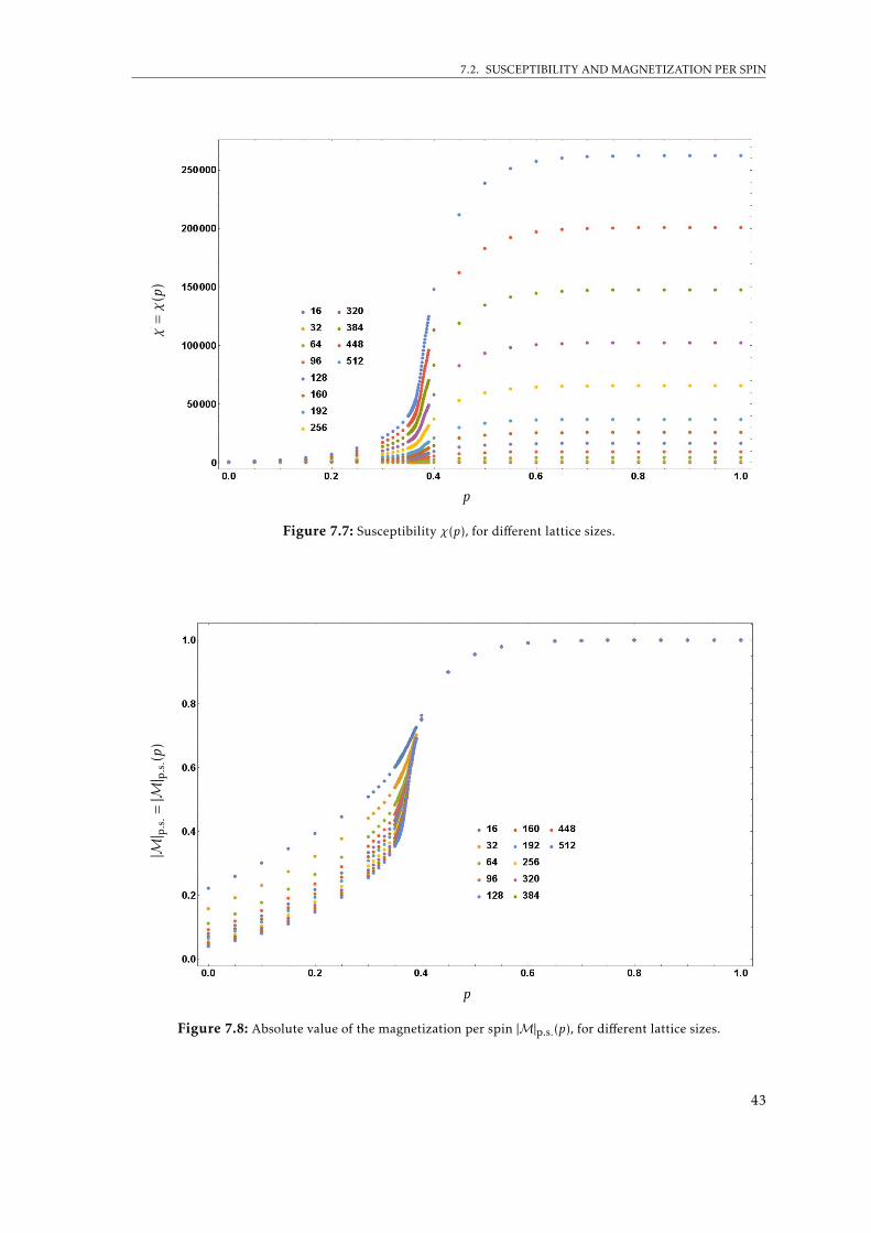
7.2. SUSCEPTIBILITY AND MAGNETIZATION PER SPIN

χ=χ

(p)

p

Figure 7.7: Susceptibility χ(p), for different lattice sizes.

|M| p.

s.=|M| p.

s.(p

)

p

Figure 7.8: Absolute value of the magnetization per spin |M|p.s.(p), for different lattice sizes.

43

CHAPTER 7. RESULTS

7.3 Correlation Function

The behavior of the correlation function Γ (r) for an Ising ferromagnet is described by

Γ (r) = 〈s0sr〉 − 〈s0〉〈sr〉. (7.2)

In Section 6.3 we reduced the F∆ model, where on each lattice site we have an integer-valued heightvariable, to a Z invariant Ising-type formulation, where hx ∈ {±1}. Hence, we can utilize the sameexpression for the correlation function (see Equation 7.2) and fit it to the most general form

Γ (r) = 〈h0hr〉 − 〈h0〉〈hr〉 ∝1rηe−

rξ , (7.3)

for different couplings p. Comparing our data with this theoretical model implies that the corre-lation length is infinite (ξ = ∞) for all p ∈ [0,1]. For p ≤ pc we obtain a rough phase with infinitecorrelation length such that the correlation function behaves as Γ (r) ∝ 1

rη . When fitting η, we wantto take into account the long-range contributions from the other side of the finite system, thereforethe ansatz is

Γ (r) ∼ c(

1rη

+1

(L− r)η

)+ d, (7.4)

for p ≤ pc. For p > pc we are entering the rigid phase, which indicates that we expect Γ (r) to ap-proach a constant, until reaching Γ (r)→ 1 for p→ 1.In the rigid phase near the critical point we include an exponential correction term to the correla-tion function, with a second order sub-leading correlation length ξ(2). Therefore the fitting ansatzis given by

Γ (r) ∼ c

e−rξ(2)

rη+e− L−rξ(2)

(L− r)η

+ d, p > pc,p ≈ pc. (7.5)

The exponential term and the power-law term vanish for increasing p, indicating that η → 0 andξ(2) →∞. For increasing coupling the constant d becomes more and more dominant, confirmingan infinite correlation (see Figure 7.9).By analyzing the correlation function we can already draw some conclusions. We have a roughphase with long-range correlation for p ≤ pc. This means that throughout this range of couplingsthe correlation function behaves like

Γ (r) ∝ 1rη, (7.6)

where η is a continuously varying critical exponent, starting at η(p = 0) ≈ 1 and reaching η(pc ≈0.36) ≈ 0.25. For p > pc we are in a rigid phase, where we have infinite correlation and therefore

Γ (r) ∝ const. (7.7)

Throughout the whole range of couplings p ∈ [0,1], we could not measure any exponential long-range contributions to the correlation function. Therefore we have an infinite correlation length(ξ =∞) for all couplings p.

44

7.4. BINDER CUMULANT

Γ(r

)

r

Figure 7.9: Correlation function Γ (r) for L = 256 and different p.

7.4 Binder Cumulant

Up to this point we estimated the critical coupling pc visually, without using a quantitative methodthat provides us with a precise numerical estimate. At this point we want to use the Binder methoddescribed in Subsection 2.6.4. We take the Binder cumulant defined as

U4 =〈(M4

A +M4B)〉

〈(M2A +M2

B)〉2(7.8)

for different lattice sizes, and calculate intersection points of consecutive lattice sizes with ratio2. Note that we measure the Binder cumulant as described in Section 6.6. We have 8 intersec-tion points which can be considered as pseudo-critical couplings pLi ,2Li (see Figure 7.10). Thesepseudo-critical couplings are plotted as a function of 1

Lmin, where Lmin = min{Li ,2Li} = Li . The

size-dependent behavior of the pseudo-critical couplings can be described very well by fitting it as

exκ + pc,Binder, (7.9)

where e,κ,pc,Binder are fit parameters. The offset pc,Binder of the fit gives a prediction for the truecritical coupling pc for L→∞, i.e., for infinite volume (see Figure 7.11).For the 3 fit parameters we obtain

e = 0.048(2), κ = 0.44(3), pc,Binder = 0.3576(5). (7.10)

45

CHAPTER 7. RESULTS

U4

p

Figure 7.10: Binder cumulant for all different lattice sizes L.

7.5 Finite-Size Scaling Procedure

in Subsection 2.6.5 we discussed the classical two-dimensional XY model near its BKT-transition.We described the finite-size scaling ansatz for the susceptibility at the critical coupling and ob-tained

χ ∝ L2−ηc (log(L))−2re , (7.11)

where ηc = 14 and re = −1

16 . Having a first accurate estimate for the critical coupling pc, we can checkwheter the finite-size scaling ansatz in Equation (7.11) can be reproduced. We take the logarithmon both sides and substitute x = log(L) such that we obtain

ln(χ) ∼ (2− η) ln(L) + (−2re) ln(ln(L)) + b

∼ (2− η)x+ (−2re) ln(x) + b. (7.12)

The additional logarithmic correction means that ln(χ) grows faster than (2 − η)x, whereas thedata on the contrary show a slower decrease. Fitting the data at pc = 0.3576 and leaving the fitparameters (η,re,b) free, leads to results

η = 0.2405(4), re = 0.0616(8), (7.13)

which are not in agreement with the predicted behavior. Fixing ηc or re leads to big deviations inthe other variable and also varying pc does not improve the fit by any means. The residues indicatethat the form (7.11) is not the correct fit for χ.Balog predicted in [20, 21] that the true finite-size scaling behavior is

ln(χ) ∼ (2− η)x+O(Q) + b

∼ (2− η)x+ aπ2

2

(x+u)2 + b, (7.14)

46

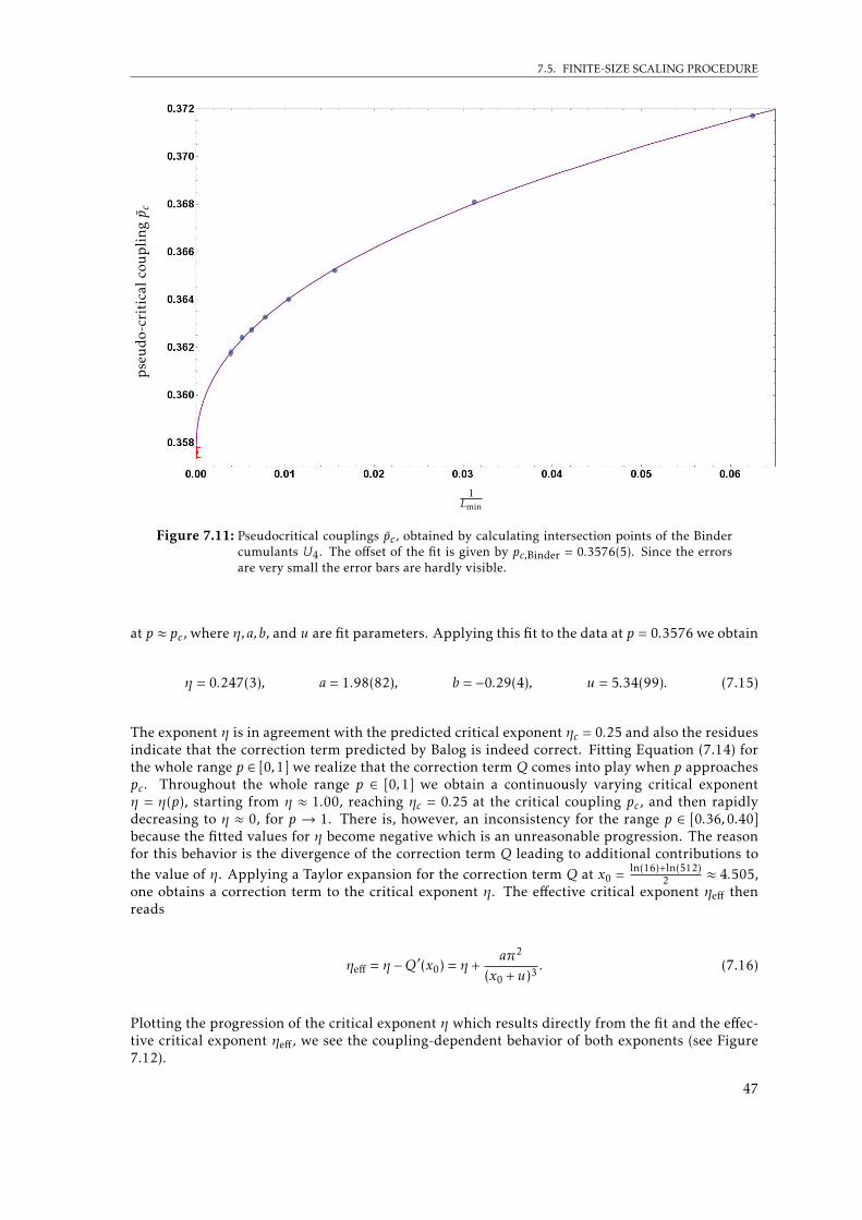
7.5. FINITE-SIZE SCALING PROCEDURE

pse

ud

o-cr

itic

alco

up

lingp c

1Lmin

Figure 7.11: Pseudocritical couplings pc, obtained by calculating intersection points of the Bindercumulants U4. The offset of the fit is given by pc,Binder = 0.3576(5). Since the errorsare very small the error bars are hardly visible.

at p ≈ pc, where η,a,b, and u are fit parameters. Applying this fit to the data at p = 0.3576 we obtain

η = 0.247(3), a = 1.98(82), b = −0.29(4), u = 5.34(99). (7.15)

The exponent η is in agreement with the predicted critical exponent ηc = 0.25 and also the residuesindicate that the correction term predicted by Balog is indeed correct. Fitting Equation (7.14) forthe whole range p ∈ [0,1] we realize that the correction term Q comes into play when p approachespc. Throughout the whole range p ∈ [0,1] we obtain a continuously varying critical exponentη = η(p), starting from η ≈ 1.00, reaching ηc = 0.25 at the critical coupling pc, and then rapidlydecreasing to η ≈ 0, for p → 1. There is, however, an inconsistency for the range p ∈ [0.36,0.40]because the fitted values for η become negative which is an unreasonable progression. The reasonfor this behavior is the divergence of the correction term Q leading to additional contributions tothe value of η. Applying a Taylor expansion for the correction term Q at x0 = ln(16)+ln(512)

2 ≈ 4.505,one obtains a correction term to the critical exponent η. The effective critical exponent ηeff thenreads

ηeff = η −Q′(x0) = η +aπ2

(x0 +u)3 . (7.16)

Plotting the progression of the critical exponent η which results directly from the fit and the effec-tive critical exponent ηeff, we see the coupling-dependent behavior of both exponents (see Figure7.12).

47

CHAPTER 7. RESULTS

η(p

),η e

ff(p

)

p

Figure 7.12: Progression of the critical exponent η. The correction term Q leads to a large discrep-ancy between η(p) and ηeff(p).

7.6 Taylor Fit

Fitting the data for χ(L) (for fixed p) to the finite-size scaling ansatz (7.14) leads to large errors inthe fit parameters (η,a,b,u), since we are fitting a function with 4 parameters to 12 data points. Wewant to use the fact that u is a non-universal constant, such that we can fix u in the vicinity of thecritical point and reduce the number of parameters to 3. Since the progression of all fit parameters(η,a,b,u) is continuous and smooth in the neighborhood of pc,Binder ≈ 0.3576, we perform a Taylorexpansion of the fit parameters around a hypothetical critical coupling pc

η(p) = ηc + η1(p − pc) +O((p − pc)2),ηc =14,

a(p) = ac + a1(p − pc) +O((p − pc)2),

b(p) = bc + b1(p − pc) +O((p − pc)2),

u(p) = uc.

Using this expansion we include several probabilities near the critical coupling pc and fit themaltogether. For this fit we were using

p ∈ {0.3560,0.3561, · · · ,0.3589,0.3590}, (7.17)

which implies that we are using 372 data points in order to fit 7 parameters (pc,η1, ac, a1,bc,b1,uc).Using the Taylor fit expansion we obtain

pc = 0.3579(1), uc = 3.39(11),

ηc = 0.25, η1 = −5.00(5),

ac = 0.82(5), a1 = 57(4),

bc = −0.238(3), b1 = −14.43(42).

The result for the critical coupling pc differs slightly from the one obtained by using the Bindermethod, but both are still consistent with each other within their statistical errors

pc,Binder = 0.3576(5) pc,Balog Fit = 0.3579(1). (7.18)

48

7.7. HELICITY MODULUS

7.7 Helicity Modulus

In Subsection 2.6.5 we described the helicity modulus, which is defined in its dimensionless formas

Υ =1T∂2

∂α2F(α)∣∣∣∣∣α=0

, (7.19)

where α is the twist angle imposed at the boundary. The helicity modulus provides a measure forthe spin stiffness of an XY model. By dualizing an XY model, we obtain a height model where thespin stiffness is described by the winding number squared W 2

x , i.e.,

Υ = 〈W 2x 〉. (7.20)

Measuring W 2x for the F∆ model, we recognize that we obtain similar numerical values for all the

different lattice sizes we take into consideration. For the sake of clarity we only plot 〈W 2x 〉(p) for

the lattice size L = 512.

〈W2 x〉

p

Figure 7.13: Winding number 〈W 2x 〉, the arrow indicates pc,Binder.

Compared to the predicted behavior in Figure 2.8, we see that we do not have a similar behaviorfor the winding number squared 〈W 2

x 〉. The reason for this is that we excluded certain configura-tions described in Subsection 6.1.2, since we are only able to sample a certain number of windingsectors (namely the ones where Wx mod 4 = 0 and Wy mod 4 = 0). Nonetheless, we also see thatthe winding number 〈W 2

x 〉 is decreasing rapidly and approaches 0 around p ≈ pc. However, nouniversal jump has been determined.

49

8 Summary and Interpretation of the

Results

Now we want to briefly discuss our results and put them into context with the classical XY modeland its BKT-transition (compare with Figure 2.7). We simulated the F∆ model, where we firstapplied the modulo 4 formulation and then mapped this formulation to an Ising-type model inorder to measure observables. The magnetization of both sublattices (MA,MB), the susceptibilityχ, and the absolute value of the magnetization per spin |M|p.s. reveal a phase transition to a rigidphase, that takes place at a certain critical coupling. Measuring the correlation function Γ (r) for p ∈[0,1] reveals that for p ∈ [0,pc] it behaves as Γ (r) ∝ 1

rη , with a continuously varying critical exponentη = η(p). For p ∈ (pc,1] we enter a rigid phase where infinite correlations arise and Γ (r) ∝ 1. Thisshows that the phase transition we are dealing with is a dual form of a BKT-transition, separatinga rough phase for p ∈ [0,pc] from an rigid one for p ∈ (pc,1]. The Binder cumulant provided a firstprecise estimate of the critical coupling pc,Binder. Fitting our data for the susceptibility χ = χ(L,p =fixed) to the finite-size scaling prediction by Balog did not only confirm our previous result forpc,Binder, but also confirmed that the exponent η at the critical point is indeed given by ηc = η(pc) =14 . The connection to the classical XY model can be made by dualizing the F∆ model. The analogueof Figure 2.7 in our case is similar but flipped (see Figure 8.1).

F∆ model (height model)

p = 0 ppc

rigid (smooth) phase, flat heightfield,ξ =∞, Γ (r) ∼ 1,

infinite correlation

Critical point pcdual BKT-transition,

ξ =∞, Γ (r) ∼ 1rηc

, ηc = 14

rough phase,continuously varying η,

ξ =∞, Γ (r) ∼ 1rη

,


p = 0 ppc

Disordered phase,

ξ <∞, Γ (r) ∼ e− rξ ,

short-range correlation

Critical point pcBKT-transition,

ξ =∞, Γ (r) ∼ 1rηc

, ηc = 14

Superfluid phase,continuously varying η,

ξ =∞, Γ (r) ∼ 1rη

,


Dualized F∆ model (generalized XY model)

Dualizing the F∆ model

Figure 8.1: F∆ model with dual BKT-transition.

51

9 Conclusion and Outlook

In this thesis we investigated the F∆ model on a honeycomb lattice, which was mentioned by Prof.Martin Hairer in 2016 at his Einstein lectures at the university of Bern. This model belongs to theclass of height models and constrains nearest-neighboring height variables to differ by ±1. We usedthe methods of the dual transformation and the star-triangle transformation to obtain the dualizedF∆ model on a honeycomb lattice, which belongs to the class of two-dimensional U (1) modelsand has a severe sign problem which prevents numerical simulations. Therefore we simulated theoriginal F∆ model, by using a modulo 4 formulation.Studying the correlation function and the susceptibility revealed a dual BKT-transition at a criticalcoupling pc. Using the Binder method, we obtained a reliable result for the critical coupling pc,which was confirmed by combining the finite-size scaling ansatz proposed by Balog with a Taylorfit around the critical point. We obtained the following results

pc,Binder = 0.3576(5) pc,Balog Fit = 0.3579(1).

Still there are open questions one would like to address. Is it possible to perform a dual trans-formation (section 5.3) without setting the coupling parameter K to zero? If so, is it possible toanalytically derive the critical coupling? Can one construct an algorithm which allows us to dy-namically enter winding sectors we could not reach before (subsection 6.1.2)? If so, is it possible tocompare the behavior of 〈W 2

x 〉 with the behavior of the helicity modulus Υ , and check its universaljump at the BKT transition?The F∆ model is an interesting height model which allows generalizations and leaves open ques-tions. In this thesis we have laid the groundwork for potential future studies.

53

Acknowledgement

It is a pleasure to thank Uwe-Jens Wiese for introducing me to this interesting topic,for his advice and patience throughout the last year. Special thanks go also to StephanCaspar. He assisted me in a variety of different tasks and always had an answer at handwhen I got stuck in a problem.

55

A Formulas

A.1 Fourier Representation

If b(k) is a function of some integer k ∈ Z, it can be represented as the integral of a 2π-periodicfunction f2π, such that

b(k) =1

2π

∫ 2π

0e−ikϕf2π(ϕ)dϕ, (A.1)

and

f2π(ϕ) =∑q∈Z

b(q)eiqϕ . (A.2)

A.2 Dirac Comb

In order to evaluate certain sums that arise in the dualization procedure we used the Dirac comb,which is a periodic tempered distribution constructed from Dirac-Delta-functions

δT (t) def.=∑k∈Z

δ(t − kT ) =1TδT (

tT

), (A.3)

for some given period T . Due to T -periodicity, the Dirac comb can be expressed as a Fourierexpansion

δT (t) =∑n∈Z

b(n)e2πin tT =

1T

∑n∈Z

e2πin tT , (A.4)

where b(n) is given by

b(n) =1T

∫ T2

− T2δT (t)e−2πin t

T dt =1T. (A.5)

A.3 Poisson Summation Formula

The Poisson summation formula reads∑µ∈Z

g(µ) =∑n∈Z

∫R

e2πinφg(φ)dφ. (A.6)

This identity is true for any function g(x), which is analytical for real values of x and for which theintegral ∫

R

e2πinφg(φ)dφ (A.7)

is absolutely convergent.

57

Bibliography

[1] M. Hasenbusch, G. Lana, M. Marcu, and K. Pinn. Cluster algorithm for a solid-on-solid modelwith constraints. Phys. Rev. B, 46(16):10472, 1992.

[2] K. Binder and D. P. Landau. A Guide to Monte Carlo Simulations in Statistical Physics. Cam-bridge University Press, 2 edition, 2000.

[3] A. Wipf. Statistical Approach to Quantum Field Theory. Springer, 2013.

[4] R. B. Potts. Some generalized order-disorder transformations. Proc. Camb. Philos. Soc., 48(106),1952.

[5] G. H. Wannier and H. A. Kramers. Statistics of the two-dimensional ferromagnet. part i. Phys.Rev., 60:252, 1941.

[6] G. H. Wannier. The statistical problem in cooperative phenomena. Rev. Mod. Phys., 17:50,1945.

[7] P. Serna, J. T. Chalker, and P. Fendley. Deconfinement transitions in a generalised XY model.J. Phys. A, 50, 2017.

[8] D. H. Lee and G. Grinstein. Strings on two-dimensional classical XY models. Phys. Rev. Lett.,55:541, 1985.

[9] S. E. Korshunov. Possible splitting of a phase transition in a 2d XY model. JETP, 41:263, 1985.

[10] R. J. Baxter. F model on a triangular lattice. J. Math. Phys., 10:1211, 1969.

[11] H. Wagner and N. D. Mermin. Absence of ferromagnetism or antiferromagnetism in one- ortwo-dimensional isotropic Heisenberg models. Phys. Rev. Lett., 17:1133, 1966.

[12] P. C. Hohenberg. Existence of long-range order in one and two dimensions. Phys. Rev., 158:383,1967.

[13] M. E. Fisher. Critical Phenomena. Academic Press London, 1971.

[14] V. Privman. Finite Size Scaling and Numerical Simulation of Statistical Systems. World Scientific,Singapore, 1990.

[15] K. Binder. Computational Methods in Field Theory. Springer, 1992.

[16] K. Binder. Finite size scaling analysis of Ising model block distribution functions. Zeitschriftfuer Physik, B43:119, 1981.

[17] J. M. Kosterlitz. The critical properties of the two-dimensional XY model. J. Phys. C: SolidState Phys., 7:1046, 1974.

[18] R. Kenna. The XY model and the Berezinskii-Kosterlitz-Thouless phase transition. "http://www.mariecurie.org/~mariecur/annals/volume4/phy4.pdf".

[19] M. Hasenbusch. The two-dimensional XY model at the transition temperature: a high-precision Monte Carlo study. J. Phys. A: Math. Gen., 38:5869, 2005.

[20] J. Balog. Kosterlitz-Thouless theory and lattice artifacts. J. Phys. A: Math. Gen., 34:5237, 2001.

59

http://www.mariecurie.org/~mariecur/annals/volume4/phy4.pdf

http://www.mariecurie.org/~mariecur/annals/volume4/phy4.pdf

Bibliography

[21] J. Balog, M. Niedermaier, F. Niedermeyer, A. Patrascioiu, E. Seiler, and P. Weisz. Does the XYmodel have an integrable continuum limit? "https://arxiv.org/abs/hep-lat/0106015v3",December 2006.

[22] M. Hasenbusch. The Binder cumulant at the Kosterlitz-Thouless transition. J. Stat. Mech.,2008.

[23] U. Gerber and W. Bietenholz. Berezinskii-Kosterlitz-Thouless transition and the Haldane con-jecture: Highlights of the physics Nobel prize 2016. "https://arxiv.org/abs/1612.06132",2017.

[24] U.-J. Wiese. Sign and complex action problems: The Potts model approximation to dense QCDas a solvable example. "http://www.wiese.itp.unibe.ch/lectures/sign.pdf", 2006.

[25] L. Onsager. Crystal statistics. i. A two-dimensional model with an order-disorder transition.Phys. Rev., 65:117, 1944.

[26] C. Domb and M. S. Green. Phase Transitions and Critical Phenomena. 1. Academic Press Lon-don, 1972.

[27] A. McIntosh. The Jackknife estimation method. "https://arxiv.org/abs/1606.00497".

60

https://arxiv.org/abs/hep-lat/0106015v3

https://arxiv.org/abs/1612.06132

http://www.wiese.itp.unibe.ch/lectures/sign.pdf

https://arxiv.org/abs/1606.00497

Selbstständigkeitserklärung

gemäss Art. 28 Abs. 2 RSL 05

Name/Vorname: Bühlmann Patrick

Matrikelnummer: 13-101-126

Studiengang: Master of Science in PhysicsBachelor 2 Master � Dissertation 2

Titel der Arbeit: Height Models on a Honeycomb LatticeLeiter der Arbeit: Prof. Dr. U.-J. Wiese

Ich erkläre hiermit, dass ich diese Arbeit selbständig verfasst und keine anderen alsdie angegebenen Quellen benutzt habe. Alle Stellen, die wörtlich oder sinngemäss ausQuellen entnommen wurden, habe ich als solche gekennzeichnet. Mir ist bekannt,dass andernfalls der Senat gemäss Artikel 36 Absatz 1 Buchstabe r des Gesetzes vom5. September 1996 über die Universität zum Entzug des auf Grund dieser Arbeit ver-liehenen Titels berechtigt ist. Ich gewähre hiermit Einsicht in diese Arbeit.

Datum/Ort: 25. April 2018 Unterschrift:3012 Bern

Bühlmann Patrick

61

Documents

Height models on a honeycomb lattice - wiese.itp.unibe.ch · model, a two-dimensional lattice model on a honeycomb lattice, is deﬁned to have an integer-valued height variable (or