Embed Size (px)
Citation preview

Hedging Retail ElectricityHedging Retail Electricity
Eric MeerdinkEric MeerdinkDirector, Structuring & AnalyticsDirector, Structuring & Analytics
Hess CorporationHess Corporation
Disclaimer: The views and methods described in this presentation are the viewsand methods of the presenter and not endorsed by Hess Corporation.

2
Risks
• Three main areas of risk in retail electricity:– Market Price Risk– Volumetric Risk– Shaping Risk
• I will be concentrating on the three risk buckets listed above. How to quantify and measure these risks, and how to hedge them.
• Other risks (not part of this talk):– Credit Risk– Operational Risk– Regulatory Risk– Market Structure Risk

3
What is the Appropriate Risk Measure?
• Why do firm’s hedge? To reduce risk and the expected costs from financial distress.
• What is risk and how do we measure it?
• What are the costs of financial distress?
• We need a quantitative measure to use as a standard to evaluate risk and evaluate any hedge structure.
• This quantitative measure industry specific and needs to fit the specifics of the business.
• I propose that Cash Flow at Risk (CF@R) and stress testing are the appropriate risk measures for a retail electricity portfolio.

4
Cash Flow at Risk (CF@R)
• Value at risk (V@R) is a probabilistic measure of the reduction in an asset’s value from adverse changes in market prices over a holding period. The holding period is typically anywhere from one day to one week.
• V@R assumes that markets are liquid and continuous. All trades can be liquidated at market prices in the measured time horizon thereby limiting losses. Also, notional contractual quantities are fixed and known.
• Cash Flow at Risk (CF@R) is a probabilistic measure of the reduction in operating cash flows through delivery from an adverse movement in market prices and usage.
• CF@R assumes that all trades are held through delivery. This allows the CF@R model to allow the contractual quantities to vary from the expected, and to be correlated with changes in market prices.

5
CF@R and Retail Contracts
• Retail load contracts are bilateral contracts between a supplier and an end user to deliver electricity and other associated products to the end user.
• Since these are contracts for the delivery of electricity they are not subject to termination and the supplier has the obligation to meet delivery.
• The contracted quantity is a forecast and not known until delivery.
• The quantity consumed by the end user is as a rule positively correlated with spot market prices.
• The market for retail electricity contracts is not liquid and continuous. All trades must be carried through delivery, and any liquidations would take longer than the typical V@R holding period.
• CF@R is a more appropriate measure of risk to use when deciding on a hedging plan and measuring risk.

6
CF@R Calculation
• The only practical method to calculate CF@R for a retail business is through simulation analysis (Monte Carlo).
• Because we are estimating cash flows through delivery we need to simulate the correlated behavior of spot prices, forward prices and customer load.
• Ideally this needs to be done at the hourly level to simulate extreme spot price behavior.
• Need to model spot prices and load with the following behavior:– Mean reversion
– Jumps and Spikes

7
Stress Testing
• CF@R is only as good as our ability to model price-load behavior.
• Historic data on the price-load relationship at the hourly level captures the major driver of load and price volatility – weather.
• Weather is the major driver of volatility, but not the only driver.
• Other drivers exist that can have large impacts on cash flows, but may have either a low probability of occurring, or difficult to model.
• One of these is the economy. Economic booms and busts can have large impacts on the demand for electricity and by consequence a large impact on price.
• Stress testing is the only practical method of calculating the impact on cash flows of economic impacts.
• Any hedging plan needs to incorporate stress testing as a basic tool to judge the effectiveness of the hedge structure.

8
Retail Structures
• There are numerous retail pricing structures:– Fixed Price Full Requirements– Fixed Price Block (customer purchases a fixed block at a fixed price)
– Floating Index (customer takes the energy at the hourly LMP)
– Block & Index (fixed block plus the remainder of the load is index)
– Hybrid (incorporate all the above)
– Triggers (customer can trigger a block purchase at a known price target)
• All of these structures have varying degrees of risk. The structure with the greatest risk for a retailer is the fixed price full requirements contract. I will concentrate my talk on this retail structure.
9
What is a Full Requirements Load Following Contract
• Full Requirements Load Following: A fixed price agreement to serve all the electricity load of a customer, and provide all products required to supply the electric load, for a pre-determined interval of time, without restrictions on volume. Typically served at a fixed rate per MWH.
• Responsible for the hourly cost to serve the load.
• Typical key products to be supplied:
– Load Following Energy
– Capacity
– Transmission
– Ancillaries
– RECs

10
Load Following Energy
• In a load following contract the supplier is obligated to supply the energy demanded (consumed) by the end-user on an hourly basis. Supply equals demand instantaneously.
• In most deregulated markets (ISOs) the cost of this energy is determined by the topology of the transmission grid and current generation costs and transmission constraints. Hence, market prices are determined hourly.
• The load following cost is the mathematical sum of price times hourly demand for all hours served.
• The next slide depicts the load shape of a “typical” end-user.

11
Load Following Energy Diagram
0
1
2
3
4
5
6
7
8
9
10
11
12
13
14
15
16
1 2 3 4 5 6 7 8 9 10 11 12 13 14 15 16 17 18 19 20 21 22 23 24
On-Peak BlockOff-Peak Block
MWH Served
Load Following MWH
Hours
MW

12
Expected Cost to Serve Load
• Model definitions:– Si = Spot price in hour i (random variable)
– Li = Load in hour i (random variable)
– Covi = Covariance between S and L in hour i Cov(Si,Li).
– i = hours in the month i = 1,…,N
– Averages will be denoted with a bar over the variable
– Expectations will be taken at time t given information available up to and including time t. Referenced by a subscript t.
N
iitt PE
NS
1
1PowerofValueForward
N
iitt LE
NL
1
1LoadExpectedofValueForward
ititit
it LE L and SE S

13
Expected Cost to Serve Load
• Cost to serve load:
• Expected cost to serve load :
• Taking expectations and solving we get:
N
iiiLS
1
Cost
N
iiitt LSEE
1
Cost
N
ii
it
it
N
iiitt LLSLSEE
11
,iSCov Cost
N
i
N
i
itt
itttt SLLLSNE
1 1
, ii LSCovCost
14
Expected Cost to Serve Load
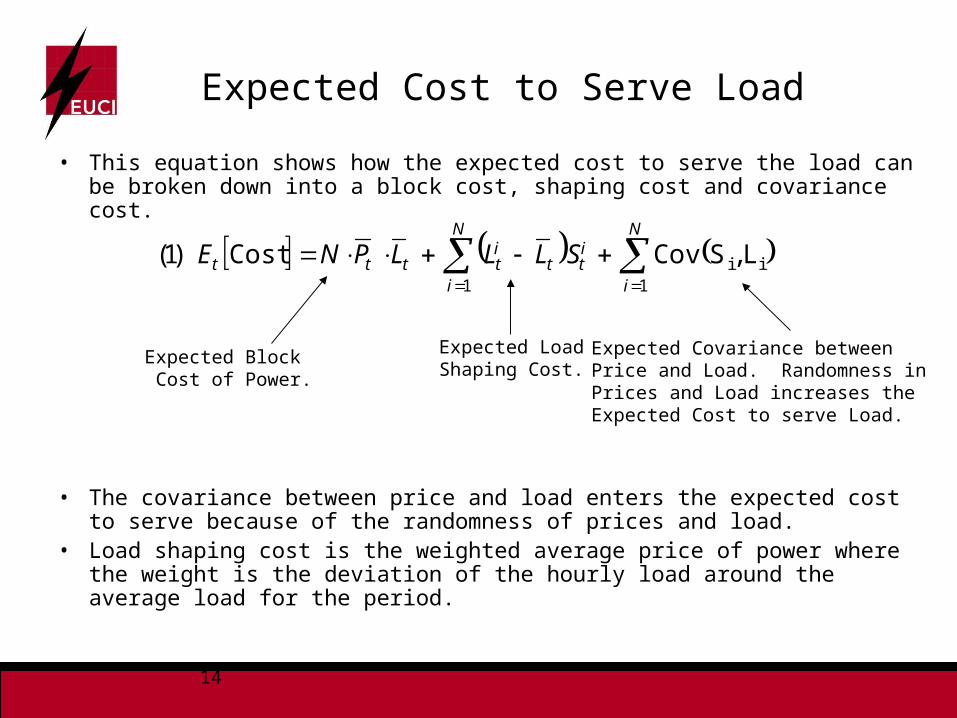
• This equation shows how the expected cost to serve the load can be broken down into a block cost, shaping cost and covariance cost.
• The covariance between price and load enters the expected cost to serve because of the randomness of prices and load.
• Load shaping cost is the weighted average price of power where the weight is the deviation of the hourly load around the average load for the period.
N
i
N
i
itt
itttt SLLLPNE
1 1
,)1( ii LSCovCost
Expected Block Cost of Power.
Expected LoadShaping Cost.
Expected Covariance betweenPrice and Load. Randomness inPrices and Load increases theExpected Cost to serve Load.

15
Expected Cost to Serve Load
• Divide equation (1) by the expected MWHs to obtain the cost per MWH.
• Divide by the forward price of power:
t
iittitt
t
t
LN
LSELLES
LNE
,iSCovCost
Forward Price ofBlock Power.
Forward Cost of Load Shapingand Load Following
tt
iittit
tt
t
LSN
LSELLE
LSN
E
,1 iSCovCost
Load Shaping Factor (SFt)

16
Expected Cost to Serve Load
tttt LNSSFE 12 Cost
The expected shaping factor, SFt , is the ratio of the sum of theexpected hourly load shaping cost plus the expected hourlycovariance cost to the expected block cost.
The shaping factor is the cost (as a percentage) above ourblock cost to cover the expected cost arising from the covariance between hourly load and price.
Equation (1) can be written as in equation (2) below.

17
Expected Profit Function
• The expected profit function for a fixed price load following contract is just the expected revenue less the expected cost.
• The expected revenue is the fixed (known) revenue rate times the expected energy.
KWh or MWh DemandEnergy Expected LN
¢/KWh or $/MWh Price) (Contract Rate Revenue R
LNSSF 1 - LNR
t
tttt
tπ)3(

18
Market Price Risk: Delta Hedging
• The objective of a hedging strategy is to create a portfolio that is riskless over a small interval of time due to changes in the random components.
• For a linear contract a delta hedge will provide a hedge against market price movements.
• I will show that a load following contract is a non-linear contract where a delta hedge will provide only a first-order approximation to changes in market prices.
• Since the cost to serve is a function not only of random prices but random loads, changes in expected load can increase or decrease expected cost.
• This section breaks down and explains the hedging components of a load following contract.

19
Delta Hedging the Expected Cost
• Start with the expected cost function, equation (1) and take a Taylor series expansion with respect to prices and loads.
• Where refers to higher order terms. Neglecting these terms we can write the change in expected cost as:
iti
t
iiti
t
iit
it
N
i
it
itt L
LCov
PPCov
PLPLE1
)4( Cost
)5(11
tt
it
N
iit
iitt
N
i t
it
it
i
t
it
titt L
LL
LCov
PPP
PPCov
P
PLLLN
Price Hedge Load Hedge
The delta on a load followingcontract does not equal 1.0
After delta hedging the price riskwe are left with the first order load riskor Gamma risk.

20
Delta Hedging the Expected Cost
• The last equation on the previous slide has two terms that need to be defined.
• The first tem represents the change in the expected price at hour i from a change in the forward price of power:
• The second term represents the change in the expected load in hour i from a change in the expected average level of load:
• Both of these quantities reflect the change in the shape of the hourly price and load shape with respect to a change in the underlying average price and load.
t
it
PP
t
it
LL

21
Delta of a Load Following Contract
• Start with equation (2):
• Take the first derivative of equation (2) with respect to price.
• Disregarding the shaping factor impact the delta of a load following contract equals:
tttt LNSSF1CostE(2)
tLNSS
SFLNSF1
S
Costt
ttt
t
t
tt LN LNSF1 Delta (6) tSΔ
In general, the delta of load following contract is greater than the notionalquantity when the shaping factor is positive. SF can be anywhere from 0%to 15%, depending on the customer type.

22
What is the Expected Load ?
• What quantity do we use to hedge?• Since load is a random variable we want to hedge the expected
quantity.• Why is load random: Weather and economic/business conditions.• Weather has a “known” distribution that can be used to calculate the
expected weather (normal weather).• Need to model load as a function of weather.• Economic/business conditions can be either specific to the industry
or customer or general economic conditions.• Business conditions specific to the customer can be estimated from
past or known customer usage patterns (plant closures, retooling).• General economic conditions include recessions and economic
boom periods.
L
23
Weather
• In the short run weather has the most volatility and has the greatest impact on electricity usage.
• Weather has a long history of data from which to imply a distribution.
• We can estimate the expected load using either of two methods:– 1. Define a normal or expected weather pattern from the data and use
the estimated load/weather function to calculate the expected load.– 2. Run the historic weather through the estimated load/weather function
to obtain estimates of the load under each year’s historic weather, and then take an average of the estimated loads.
• The result is a weather normalized load estimate.• Question: What is the proper historic period to use?• Answer: No agreed upon standard.• The NWS uses a 30-year normal updated every decade. Weather
derivative markets use a 10-year average.

24
Economic and Business Conditions
• Usage conditions specific to the customer or industry can be applied after the load has been weather normalized.
• Specific conditions include planned shutdowns for maintenance and retooling. This type of information can be obtained from the customer or from past usage.
• Other specific conditions can arise from an expansion in a customer’s load from favorable economic or business conditions, such as an expansion of a service line or warehouse space.
• General economic growth conditions can effect all customers, but is not specific to a particular customer. Need to account for expected load growth (reductions) from growth (decline) in the national or regional economy.

25
Volumetric Risk
• After delta hedging the market price risk we are left with the first order load risk or Gamma risk:
• Gamma risk is a volumetric risk.
• Volumetric risk (or Swing risk) is defined as a cash flow risk caused by deviations in delivered volumes compared to expected volumes. The primary cause of these volumetric deviations is weather and economic conditions.
• The delivered volumes cause a loss when the deviations in volume are positively correlated with market prices.
tt
it
N
iit
iit L
LL
LCov
P
1
CostEt

26
Long-Run Demand in PSE&G
0
1,000
2,000
3,000
4,000
5,000
6,000
7,000
8,000
6/1
/05
9/1
/05
12
/1/0
5
3/1
/06
6/1
/06
9/1
/06
12
/1/0
6
3/1
/07
6/1
/07
9/1
/07
12
/1/0
7
3/1
/08
6/1
/08
9/1
/08
12
/1/0
8
3/1
/09
6/1
/09
9/1
/09
12
/1/0
9
3/1
/10
6/1
/10
9/1
/10
12
/1/1
0
Date
MW
CoolSummer
Summer
Winter
HotSummer
Recession
June 2005 to December 2010

27
Long-Run Correlation Between Price and Load
4,800
4,900
5,000
5,100
5,200
5,300
5,400
5,500
May-06 Sep-06 Jan-07 May-07 Sep-07 Jan-08 May-08 Sep-08 Jan-09 May-09 Sep-09 Jan-10 May-10 Sep-10
Month/Yr
MW
$0.00
$10.00
$20.00
$30.00
$40.00
$50.00
$60.00
$70.00
$80.00
$90.00
$/M
WH
MW
$/MWH
12-Month Rolling Average of Load and Price in PSE&G Zone

28
Short-Run Correlation Between Price and Load
$0.00
$20.00
$40.00
$60.00
$80.00
$100.00
$120.00
$140.00
$160.00
$180.00
$200.00
07/12/10 07/13/10 07/14/10 07/15/10 07/16/10 07/17/10
$/M
WH
0
2,000
4,000
6,000
8,000
10,000
12,000
MW
Hourly Load and Price in PSE&G Zone 7/12/10 to 7/17/10
Load (MW)
Price ($/MWH)

29
Sources of Swing Risk in Load FollowingP
ower
Pric
e $
/MW
H
Demand (MW)
DispatchCurveEconomic Impact (A to B)
Weather Impactbetween a and b.
AB
a
b
Weather – Principal source of swing risk.
General Economic Conditions

30
What is Swing Risk?
• Spot prices and quantities are positively correlated.
• When quantity and prices both increase the cost to serve load increases. Profit not only becomes negative, but decreases at an increasing rate with an increase in prices.
• When quantity and prices both decrease the cost to serve load decreases. Profit becomes positive, but increases at a decreasing rate as prices decrease.
• Unlike a typical short sale, the short retail sale is non-linear.
• When hedged with a linear instrument, the resulting position is negative and non-linear.

31
Retail Sale and Long Hedge
Long HedgeSwap (Linear)
Short Sale
$/MWH
Short Retail SaleNon-linear
-
$
Net: Swing Risk “Gamma”
+
Curvature is the product of thepositive correlation between price and load.
P&
L

32
Change in Cash Flow
Load less than expected load
Load equals expected load
Load greater than expected
load
Price less than expected price - 0 +
Price equals expected price 0 0 0
Price greater than expected
price+ 0 -
LongPosition
ShortPosition
HedgedSwing Risk- - - - - -

33
Shaping Factor Risk
N to i hours for LSCost ii
N
i 1
N
i 1ii SLLLPNCost
Can be written as follows after some manipulation:
Cost Function:
Adding zero to the above equation we get the following equation:
N
i 1
S - SLLLPNCost ii
Covariance Function

34
Shaping Factor Risk
SLLs
SLLS
N Cost Shaping
N LSN Cost
σ
Standard Deviation of Hourly Price Standard Deviation of Hourly Load
Hourly Correlation between Price and Load
Hourly shaping cost is a function of the covariance between price and load.
How do we hedge this correlation risk?

35
Increase in Shaping Factor Cost
Long Hedge
$/MWH
-
$
Expected Short SaleRealized Short Sale
Expected Net Position
Realized Net Position
An increase in the shaping factor shifts theshort sale curve downward, and the resultingnet position shifts downward. The net positionis negative at all price outcomes.
+
P&
L

36
Decrease in Shaping Factor Cost
Long Hedge
$/MWH
-
$
Expected Short SaleRealized Short Sale
Expected Net Position
Realized Net Position
An decrease in the shaping factor shifts theshort sale curve upward, and the resultingnet position shifts upward. The net positionis positive at current price levels, but still hasnegative risk exposure.
P&
L
+
37
Fair Value of a Load Following Contract
• A fair price or fair value contract has an expected value of zero.
• Fair value contracts require the inclusion of the expected value of the covariance between price and load, not just the expected hourly shaping cost. Excluding this cost component biases the distribution to the left.
• But inclusion of the expected covariance in the contract price does not guarantee that the swing risk has been minimized or removed. It only guarantees that the contract is priced fairly.
• We are still left with the negative tail risk from large positively correlated price and load movements.

38
3020100-10-20-30-40-50-60
0.04
0.03
0.02
0.01
0.00
Cash Flow
De
nsi
ty
Cash Flow Distribution: Swing Risk vs. Swing Cost
Negative Skew:
Swing Risk
Swing Cost
Excluding the expected covariance produces a distributionwith a negative expected value.
Mean

39
Volumetric Hedging
• Minimum Variance Hedge
• Options– Synthetic Gamma Hedge
• Slice of System– Gamma Hedge and Shaping Factor Hedge
• Rate Design (T&C’s)

40
Minimum Variance Hedge

41
Minimum Variance Hedge• Find the hedge quantity that minimizes the variance of the profit (CF@R)
function.
• Other alternatives, not considered here, are VAR and mean-variance methods.
• Expected profit function: , Equation (3).
• Take the total differential of the profit function and add a hedge consisting of h power swaps.
• Now set the derivative of the variance with respect to h to zero and solve for h.
ttt
tt
t
t ShdSdS
CostLd
L
CostNRd
t)7(
0
hdE 2
π
)SE(d
)LdSE(dRN
L
CostCosth(8)
2t
tt
t
t
t
t
S
tt CostLNR t

42
Minimum Variance Hedge
• We can simplify this equation to:
• Where equals the correlation between expected load and expected price.
• The standard deviations are for expected load and expected price.
• The first term in the equation is the price hedge defined in equation (6).
• The second term is the correction to this hedge to take into account the correlation between price and load.
• If the correlation is zero then the optimal hedge is the traditional price hedge.
P
L
t
t
t
t NRL
Cost
S
Costh
)9(

43
Minimum Variance Hedge
• Using the optimal hedge the residual unhedged variance is equal to:
• If the correlation between expected load and expected price equals 1 or -1 then the residual unhedged variance equals zero. We have eliminated any risk over period dt.
• If the correlation equals zero, then the residual unhedged variance equals the full amount of the load effect.
• The greater the correlation the greater the effectiveness of the hedge.
dt1L
Cost 2L
2
t
t σρdE
2
2

44
Minimum Variance Hedge: Application
• We need to determine the relationship between expected price and load.• If there is a linear relationship then we can estimated the following
equation using OLS.
• The coefficient on expected price, beta, is equal to
• The change in load can then be calculated as
• We can now rewrite the hedge quantity for load as the following quantity of MWs.
ttt S L
S
L
tt SdLdS
L
S
L
NRSSF1LNSF1 h (10) tttt

45
Minimum Variance Hedge: Application
0 ρ if 0
0 ρ if 0
0 ρ if 0
NRSSF1 ttS
L
• The first part of this equation is the negative of the expected margin. Sine margin is usually positive this quantity will be negative.
• The standard deviations are positive.• If the correlation between expected load and prices is positive, then the
optimal hedge adjustment is a negative quantity. • Need to take on a short position to hedge the change in expected load.
Since price and quantity are positively correlated, a change in expected quantity will create a long position in the load following contract. The optimal hedge is then a short position.
• If the correlation is negative then the optimal hedge adjustment is a positive quantity. Need to go long. Since price and quantity are negatively correlated, a change in expected quantity will create a short position in the load following contract.

46
Example Regression Output On-Peak PSE&G FP Contract
Regression StatisticsMultiple R 87.27%R Square 76.16%Adjusted R Square 75.61%Standard Error 417.5841127Observations 445
ANOVAdf SS MS F Significance F
Regression 10 241771008.8 24177100.88 138.6488552 2.4513E-128Residual 434 75679397.18 174376.4912Total 444 317450406
Coefficients Standard Error t Stat P-valueIntercept 3,698.5486 64.27 57.55 0.00%LMP 7.1820 0.83 8.64 0.00%Mar_P -4.9284 1.02 -4.81 0.00%Apr_P -6.7488 1.01 -6.68 0.00%May_P -5.8316 0.96 -6.08 0.00%Jun_P 6.4907 0.73 8.94 0.00%Jul_P 11.8957 0.73 16.30 0.00%Aug_P 10.2282 0.77 13.28 0.00%Sep_P 4.6888 0.84 5.61 0.00%Oct_P -2.2002 0.92 -2.38 1.77%Nov_P -3.5755 0.99 -3.62 0.03%
Interactive dummy variables
A $1 change is pricesEquals a 7 MW changein average daily peak load.
19.08 11.90 7.18 S
LJuly

47
Hedge Calculation
• Using the results of the regression output and equation (10) we can estimate the minimum variance hedge position.
• Use July 2010 as an example for PSE&G FP Contract
– SF = 5%
– N = 336
– L = 3,700 MW
• Hedge 3,885 MWs less 19 MWs for each dollar of margin.
33619.08margin 3363,885 h
33619.08margin 3,700336(1.05) h

48
Static Option Hedge

49
P
Cha
nge
in P
&L
+
-
gamma
HedgeHow do we create this hedge?
Monthly Average
Price $/mwh
P
Short Gamma Hedge

50
Creating a Gamma Position from Options
P
Use vanilla calls and puts to construct the gamma position.
Cha
nge
in P
&L
+
-
Monthly Average
Price $/mwh
P ˆ

51
Theoretical Model
• It has been shown that a static hedge of plain vanilla options and forwards can be used to replicate any European derivative (Carr and Chou 2002, Carr and Madan 2001).
• Any twice continuously differentiable payoff function, , of the terminal price S can be written as:
• Our payoff function is the terminal profit. It can be decomposed into a static position in the day 1 P&L, initially costless forward contracts, and a continuum of out-of-the-money options. F0 is the initial forward price.
)(Sf
0
0
0000
F
FdKKSKfdKSKKfFSFfFfSf (11)
InitialP&L
DeltaPosition
Gamma Hedge: “Swing Risk”

52
Theoretical Model
• The initial value of the payoff must be the cost of the replicating portfolio.
• Where P(K,T) and C(K,T) are the initial values of out-of-the-money puts and calls respectively.
• Interpretation of term within the integral: Second derivative of the payoff function representing the quantity of options bought or sold.– R = Fixed revenue rate
– SF = Shaping Factor
– L(S) = MWH, function of S (spot price of power)
0
0,,
0000
F
FrT dKTKCKfdKTKPKfeFfFV
SLSSFRSf 1
SLSFKf 12

53
Solving for the Estimated Gamma Function
• Select a series of strikes, Ki , and quantities, , to create a portfolio of puts and calls.
• To estimate the gamma function we need to choose the amount of options for each strike, , so as to minimize the distance between the estimated gamma function and the true gamma function.
• Estimated gamma function equals:
• Choose the optimal quantities by minimizing the sum of the squared errors between the true and estimated gamma function over a set of Q prices.
i
i
i
M
iii
N
ii PKMaxKPMaxP
11
0,0,ˆ (12)
2
1
ˆmin
Q
jjj PP
(13)

54
Estimating the Gamma Function
• Need to estimate the relationship between load and price.• Use historic data to estimate the following regression equation.
• The data for this equation is average load (peak, off-peak) and average price (peak, off-peak). LMP is the price, D is a monthly dummy variable, and DXLMP is an interactive dummy variable with price.
• Next set up a portfolio of a short load sale and a long hedge using monthly forwards. The fixed rate on the load sale equals the RTC cost of serving the load ($/MWH).
• Use the relationship estimated in the regression equation to vary the average monthly load with respect to a change in average monthly price. Use this to estimate the gamma function.
11
1
11
1i itiiiitt lmpDDlmpLoad

55
Example Regression Output On-Peak PSE&G FP Contract
Regression StatisticsMultiple R 87.27%R Square 76.16%Adjusted R Square 75.61%Standard Error 417.5841127Observations 445
ANOVAdf SS MS F Significance F
Regression 10 241771008.8 24177100.88 138.6488552 2.4513E-128Residual 434 75679397.18 174376.4912Total 444 317450406
Coefficients Standard Error t Stat P-valueIntercept 3,698.5486 64.27 57.55 0.00%LMP 7.1820 0.83 8.64 0.00%Mar_P -4.9284 1.02 -4.81 0.00%Apr_P -6.7488 1.01 -6.68 0.00%May_P -5.8316 0.96 -6.08 0.00%Jun_P 6.4907 0.73 8.94 0.00%Jul_P 11.8957 0.73 16.30 0.00%Aug_P 10.2282 0.77 13.28 0.00%Sep_P 4.6888 0.84 5.61 0.00%Oct_P -2.2002 0.92 -2.38 1.77%Nov_P -3.5755 0.99 -3.62 0.03%
Interactive dummy variables
A $1 change is prices equals a 7 MW change in average daily peak load.For July the change equals 19.08 = 7.18 + 11.90.
19.08 11.90 7.18 L
S

56
Hedge Calculation: Theoretical Calculation
• Using the results of the regression output and equation (11) we can estimate the “optimal” static hedging position.
• “Closed form” type solution.
• Use July 2010 as an example for PSE&G FP Contract
– SF = 5%
– N = 336
– L = 3,700 MW
dKdFfSf
Ff
Ff
0
0
F
0 F0 KS33640 K S-K33640 F-S3363,885
MW) (40 MWH 13,463 19.08336(1.05)2 SL
NSF12
MW) (3,885 MWH 1,305,360 3,700336(1.05) LNSF1
)()(
)(
)(
0
0
0

57
Interpretation
• Delta hedge is 1.05 times the expected load. Buy 3,885 MWs of costless forward contracts.
• Volumetric hedge is 40 MWs for each $1 movement away from the current forward price F0.
• Purchase calls and puts (straddle and strangles) in 40 MW increments for each strike. Strikes are $1 increments away from the current forward price.
• Sum of the option costs is the Swing or Volumetric hedge cost.
• Doing this for the July 2010 PSEG FP Contract as of February 9, 2009 results in an estimated volumetric cost of $1.89/MWH.
• The next slide depicts the estimated gamma function.

58
-$2,000
$0
$2,000
$4,000
$6,000
$8,000
$10,000
$12,000
$14,000
$16,000
$18,000
$20,000
$0.00 $20.00 $40.00 $60.00 $80.00 $100.00 $120.00 $140.00
Market Price
Ch
an
ge
in
P&
L (
$0
00
)
-Gamma
Estimate
Cost as of February 9, 2009.
Estimated gamma function for July 2010 PSE&G FP load.The option cost equals $1.89/MWH per MWH served.
Example of a Gamma Function Estimate

59
Options in Practice
• While this is theoretically correct, it is not a practical method to price and hedge the volumetric risk.
• First: Market is not liquid enough to carry out the theoretical hedge.
• Second: Just calculating the dollar amount and charging the customer does not reduce the risk. An adder will just shift the distribution to the right, increasing the expected profit but not reducing the risk.
• Need to purchase the options to reduce the volumetric risk.
• Need to find a market executable option positions. This requires a discrete position in straddles and strangles.
• Need to look for executable quantities (25MW blocks or larger).
• Cannot hedge deal by deal, only practical for a portfolio.

60
Minimizing Cash Flow at Risk
• In practice we cannot purchase options in such a way as to create the smooth curves depicted earlier. Instead we need to find discrete strikes so as to minimize the “swing risk”.
• Swing risk is here defined as Cash Flow at Risk (CF@R). I am defining CF@R as the difference between the mean of the distribution and the 5th percentile.
• Since we cannot perfectly hedge the swing risk by purchasing a continuum of options we need another objective risk minimization strategy.
• Use as a strategy the minimization of the CF@R or an objective level for the CF@R. An example would be to reduce the CF@R by 50%.

61
Reduce Cash Flow at Risk
3020100-10-20-30-40-50
0.06
0.05
0.04
0.03
0.02
0.01
0.00
X
Density
Accountnig or Actuarial w ith Options
Accounting Model
Cash Flow
Swing RiskReduced
Delta Hedged
Hedged with
Options
Reduce Cash Flow at Risk

62
Methodology
• Use Monte Carlo simulation to model the load following contract and all hedges.
• Run the model to estimate the expected cost to serve the load and establish the fair price of the contract.
• Layer in delta hedges to estimate the cash flow distribution and estimate the CF@R.
• Determine the amount of risk to be minimized. This is a management decision. Cut the CF@R by 50%.
• Determine the portfolio of available options in the market.• Use an available optimization routine to determine the optimal option
portfolio that meets the required risk criteria.• Or, try multiple strategies to determine the option strategy that meets
your firm’s risk criteria.
63
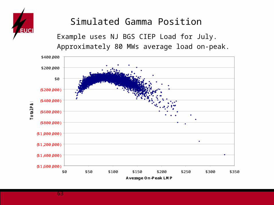
Simulated Gamma Position
($1,600,000)
($1,400,000)
($1,200,000)
($1,000,000)
($800,000)
($600,000)
($400,000)
($200,000)
$0
$200,000
$400,000
$0 $50 $100 $150 $200 $250 $300 $350
Average On-Peak LMP
To
tal P
&L
Example uses NJ BGS CIEP Load for July.
Approximately 80 MWs average load on-peak.

64
Cash Flow Distribution
Swing Risk
NJ BGS CIEP Load for July

65
Cash Flow Distribution with Swing Hedge
Swing Risk Removed
NJ BGS CIEP Load for July.
Objective was to reduce CF@R by 50%.

66
Efficient Frontier Analysis
($1,200,000)
($1,000,000)
($800,000)
($600,000)
($400,000)
($200,000)
$0
$0 $200,000 $400,000 $600,000 $800,000 $1,000,000 $1,200,000
Option Cost
5th
Pe
rce
nti
le
+/- 10% Strangle
+/- 30% Strangle
The efficient frontier tells what the minimum option costwould be to achieve a particular level of the 5th percentile.

67
Slice of System

68
Slice of System Hedge
• Bilateral contract (swap) for the purchase of a fixed percentage of a known and published load shape settled at a fixed price at a known and published node (bus or hub).
• Characteristics:– The volume is not fixed, but varies with the known load shape.
– Pricing is fixed.
– Mirror image of what is sold to the retail customer.
• Can be sold as a swap on the load shape, or the buyer of the shape can sell back the block load and have left the residual gamma payoff.

69
How do we Hedge Correlation Risk?
• Hourly shaping risk is a function of three factors:
– Hourly correlation between load and price
– Hourly standard deviation of price
– Hourly standard deviation of load
• How do we hedge these three factors?
• Are there commercially available products?
• The typical linear products and also non linear products (options) do not hedge this risk. The correlation exposure is do to underlying hourly price and load behavior which is not represented by options, even hourly options.
• Standard deviations are also not traded products ant not reducible to the typical linear and non linear products.

70
Slice of System Hedge
• The slice of system hedge is a mirror image of the short retail sale (to a degree).
• Since the hedge will not be written on the exact same load, the hedge will always be imperfect. The degree of imperfection is a function of the correlation between the retail load and the hedge load definition.
• The closer the correlation between the hedge load and the retail load the better the hedge performance (same for the settlement pricing index).
• The next slide demonstrates the net hedge position.• As the retail load changes shape, the hedge load ought to change
also if the drivers of the shape change are the same for both loads. • Hence, swing and shaping risk are more perfectly hedged with a
slice of system product.

71
$/MWH
Short Retail Sale
+
-
$ Slice of Load Hedge
Net
Slice of System Hedge

72
$/MWH
+
-
$ Slice of Load Hedge
Net
Slice of System Hedge: with Block Sale
Block Sale

73
Slice of System Pricing Factors
• Need to examine how the two load shapes and pricing nodes are correlated.
• How are the three factors correlated– Price
– Load
– Shaping Factor
• No closed form solution, need to use simulation analysis to understand the complexity of this structure.
• Required is a load shape and pricing node that are “highly” correlated with the portfolio.

74
Methodology
• Run portfolio without the slice of load to determine the CF@R.• Run the slice of system with the portfolio to determine the new
CF@R.• Determine by how much the load shape decreases the CF@R in
the portfolio.– Does it reduce the CF@R by the required amount?
– Adjust volume, load zone or pricing zone.
– The amount by which the hedge reduces the risk is a benchmark against which the load shape can be priced.
• No objective market.

75
Benefits of a Slice of System
• This trade hedges all aspects of the retail trade:– Delta Hedge (Market Price Risk)
– Volumetric Hedge (Swing Risk)
– Shaping Factor Hedge (Shaping Factor Risk)
• This product also has some cons:– It is not a liquid product in the market.
– Is a structured product. Customized.
– Fewer sellers in the market. The natural sellers are generation owners.
– Can be “expensive”.
76
Rate Design

77
Rate Design as a Risk Minimization Tool
• Rate design can also be a tool used to minimize risk in a retail contract.
• Careful design of the terms and conditions in a contract can serve to reduce risk.
• An example would be the use of usage band in a contract to protect the supplier from volumetric risk.
• Any usage by the customer outside the bands would result in the customer paying for any excess costs not collected in the contracted energy rate.
• The supplier needs to determine the amount of risk to be borne by the firm and how much can be transferred to the customer. As much a risk management decision as well as a competitive issue.

78
References
• Carr P and Madan R, Optimal Positioning in Derivative Securities, Quantitative Finance Volume 1, 2002
• Carr P and Chou A, Hedging Complex Barrier Options, working paper, 2002• De Martini P, A Survey of Volumetric Risk, The Risk Desk, Volume II No. 4 • Humphreys B, and Gill R, Using a square peg, Energy Risk, April 2004• Kilinger A, Delta hedging the load serving deal, Energy Risk, September 2006• Kolos S, and Mardanov K, Pricing volumetric risk, Energy Risk, October 2008• Oum Y, Oren S, Deng S, Hedging Quantity Risks with Standard Power
Options in a Competitive Wholesale Electricity Market, Navel research Logistics, Vol. 53, July 2006
• Oum y, Oren S, Optimal Static Hedging of Volumetric Risk in a Competitive Wholesale Electricity Market, May 2007
• Renne G, and Truesdell K, Volume Risk, Energy Politics, Issue IV, Spring 2008
• Spencer L, The Risk that Wasn’t Hedged: So What’s Your Gamma Position?, October 2001

79
Contact Info
Eric MeerdinkDirector, Structuring & Analytics
Hess CorporationOne Hess Plaza
Woodbridge, NJ 07095