Embed Size (px)
Citation preview

arX
iv:1
511.
0336
7v1
[co
nd-m
at.q
uant
-gas
] 1
1 N
ov 2
015 I
Departamento de Fısica de Materiales
Collective properties ofquantum matter: from
Hawking radiation analogues toquantum Hall effect in
graphene
Propiedades colectivas de lamateria cuantica: desdeanalogos de radiacion deHawking hasta efecto Hall
cuantico en grafeno
Juan Ramon Munoz de Nova
Tesis supervisada por Ivar Zapata Olson-Lunde y FernandoSols Lucia

II
Contents
Resumen en espanol 7
Abstract 11
I Gravitational analogs in Bose-Einstein condensates 17
1 Hawking radiation in Bose-Einstein condensates 19
1.1 Introduction . . . . . . . . . . . . . . . . . . . . . . . . . . . . . . . . . . . 191.2 Physical model . . . . . . . . . . . . . . . . . . . . . . . . . . . . . . . . . 20
1.2.1 Gross-Pitaevskii and Bogoliubov-de Gennes equations . . . . . . . 201.2.2 1D mean-field regime . . . . . . . . . . . . . . . . . . . . . . . . . . 251.2.3 Black holes in Bose-Einstein condensates . . . . . . . . . . . . . . 271.2.4 Hawking effect . . . . . . . . . . . . . . . . . . . . . . . . . . . . . 30
1.3 Typical black-hole configurations . . . . . . . . . . . . . . . . . . . . . . . 311.3.1 Flat profile . . . . . . . . . . . . . . . . . . . . . . . . . . . . . . . 311.3.2 Delta-barrier configuration . . . . . . . . . . . . . . . . . . . . . . 321.3.3 Waterfall configuration . . . . . . . . . . . . . . . . . . . . . . . . . 321.3.4 Resonant configurations . . . . . . . . . . . . . . . . . . . . . . . . 32
2 Birth of a quasi-stationary black hole in an outcoupled Bose-Einstein
condensate 35
2.1 Introduction . . . . . . . . . . . . . . . . . . . . . . . . . . . . . . . . . . . 352.2 The model . . . . . . . . . . . . . . . . . . . . . . . . . . . . . . . . . . . . 362.3 Preliminary remarks. . . . . . . . . . . . . . . . . . . . . . . . . . . . . . . 372.4 Ideal optical lattice . . . . . . . . . . . . . . . . . . . . . . . . . . . . . . . 39
2.4.1 Analysis of the simulations . . . . . . . . . . . . . . . . . . . . . . 402.4.2 Quasi-stationary regime . . . . . . . . . . . . . . . . . . . . . . . . 44
2.5 Gaussian-shaped optical lattice . . . . . . . . . . . . . . . . . . . . . . . . 492.5.1 Location of the sonic horizon and related properties . . . . . . . . 53
III
IV CONTENTS
2.6 Preliminary results for Hawking spectrum . . . . . . . . . . . . . . . . . . 572.7 Conclusions and outlook . . . . . . . . . . . . . . . . . . . . . . . . . . . . 63
3 Quantum signatures of spontaneous Hawking radiation 65
3.1 Introduction . . . . . . . . . . . . . . . . . . . . . . . . . . . . . . . . . . . 653.2 General signatures of quantum behavior . . . . . . . . . . . . . . . . . . . 673.3 General properties of Cauchy-Schwarz inequalities and Peres-Horodecki cri-
terion . . . . . . . . . . . . . . . . . . . . . . . . . . . . . . . . . . . . . . 673.3.1 Quadratic Cauchy-Schwarz violations and the generalized Peres-
Horodecki criterion . . . . . . . . . . . . . . . . . . . . . . . . . . . 723.3.2 Quartic Cauchy-Schwarz violations and entanglement . . . . . . . 72
3.4 Criteria for detection of spontaneous Hawking radiation . . . . . . . . . . 733.4.1 Cauchy-Schwarz inequalities and generalized Peres-Horodecki cri-
terion in analog Hawking radiation . . . . . . . . . . . . . . . . . . 733.4.2 Final remarks . . . . . . . . . . . . . . . . . . . . . . . . . . . . . . 76
3.5 Experimental detection schemes . . . . . . . . . . . . . . . . . . . . . . . . 773.5.1 Correlation between phonon and atomic time-of-flight signals. . . . 783.5.2 Density-density correlations . . . . . . . . . . . . . . . . . . . . . . 81
3.6 Numerical results . . . . . . . . . . . . . . . . . . . . . . . . . . . . . . . . 853.6.1 Time-of-flight detection . . . . . . . . . . . . . . . . . . . . . . . . 863.6.2 Density-density correlations . . . . . . . . . . . . . . . . . . . . . . 88
3.7 Conclusions and outlook . . . . . . . . . . . . . . . . . . . . . . . . . . . . 89
4 Time-dependent study of a black-hole laser in a flowing atomic conden-
sate 93
4.1 Introduction . . . . . . . . . . . . . . . . . . . . . . . . . . . . . . . . . . . 934.2 Black-hole laser configurations . . . . . . . . . . . . . . . . . . . . . . . . 94
4.2.1 Unstable modes . . . . . . . . . . . . . . . . . . . . . . . . . . . . . 954.2.2 Non-linear stationary solutions . . . . . . . . . . . . . . . . . . . . 97
4.3 Numerical results . . . . . . . . . . . . . . . . . . . . . . . . . . . . . . . . 984.3.1 Long-time stationary state . . . . . . . . . . . . . . . . . . . . . . 994.3.2 Continuous emission of solitons . . . . . . . . . . . . . . . . . . . . 101
4.4 Discussion and comparison with optical lasers . . . . . . . . . . . . . . . . 1064.5 Conclusions and outlook . . . . . . . . . . . . . . . . . . . . . . . . . . . . 108
II Thermal clouds 109
5 Thermal decay in a trapped gas 111
5.1 Introduction . . . . . . . . . . . . . . . . . . . . . . . . . . . . . . . . . . . 1115.2 Physical setup . . . . . . . . . . . . . . . . . . . . . . . . . . . . . . . . . . 1125.3 Classical description . . . . . . . . . . . . . . . . . . . . . . . . . . . . . . 1125.4 Quantum description . . . . . . . . . . . . . . . . . . . . . . . . . . . . . . 117
5.4.1 Equilibrium properties . . . . . . . . . . . . . . . . . . . . . . . . . 1175.4.2 Local density approximation . . . . . . . . . . . . . . . . . . . . . 118
CONTENTS V
5.4.3 Harmonic oscillator . . . . . . . . . . . . . . . . . . . . . . . . . . . 1195.4.4 Dynamical evolution . . . . . . . . . . . . . . . . . . . . . . . . . . 122
5.5 Discussion of the approximations . . . . . . . . . . . . . . . . . . . . . . . 1275.5.1 Local density approximation . . . . . . . . . . . . . . . . . . . . . 1285.5.2 Role of interactions . . . . . . . . . . . . . . . . . . . . . . . . . . . 1305.5.3 Pulse evolution . . . . . . . . . . . . . . . . . . . . . . . . . . . . . 1325.5.4 Classical-quantum correspondence . . . . . . . . . . . . . . . . . . 133
5.6 Extension of the model . . . . . . . . . . . . . . . . . . . . . . . . . . . . . 1365.6.1 Dirac picture . . . . . . . . . . . . . . . . . . . . . . . . . . . . . . 1375.6.2 General case . . . . . . . . . . . . . . . . . . . . . . . . . . . . . . 140
5.7 Experimental data . . . . . . . . . . . . . . . . . . . . . . . . . . . . . . . 1415.8 Conclusions and outlook . . . . . . . . . . . . . . . . . . . . . . . . . . . . 145
III Quantum Hall effect on graphene 147
6 Collective modes of the phase diagram of the ν = 0 quantum Hall state149
6.1 Introduction . . . . . . . . . . . . . . . . . . . . . . . . . . . . . . . . . . . 1496.2 Physical model of bilayer graphene . . . . . . . . . . . . . . . . . . . . . . 1506.3 Effective model and mean-field phase diagram . . . . . . . . . . . . . . . . 153
6.3.1 Projection onto the lowest Landau Level . . . . . . . . . . . . . . . 1536.3.2 Hartree-Fock approximation and phase diagram . . . . . . . . . . . 154
6.4 Collective modes . . . . . . . . . . . . . . . . . . . . . . . . . . . . . . . . 1586.4.1 Correlation functions and the time-dependent Hartree-Fock approx-
imation . . . . . . . . . . . . . . . . . . . . . . . . . . . . . . . . . 1586.4.2 Dispersion relation . . . . . . . . . . . . . . . . . . . . . . . . . . . 163
6.5 Monolayer graphene . . . . . . . . . . . . . . . . . . . . . . . . . . . . . . 1756.5.1 Effective Hamiltonian . . . . . . . . . . . . . . . . . . . . . . . . . 1766.5.2 Mean-field phase diagram . . . . . . . . . . . . . . . . . . . . . . . 1776.5.3 Collective modes . . . . . . . . . . . . . . . . . . . . . . . . . . . . 178
6.6 Effects of Landau-level mixing . . . . . . . . . . . . . . . . . . . . . . . . . 1806.7 Experimental remarks . . . . . . . . . . . . . . . . . . . . . . . . . . . . . 1846.8 Conclusions and outlook . . . . . . . . . . . . . . . . . . . . . . . . . . . . 184
IV Global conclusions 187
7 Global conclusions and future perspectives 189
V Appendices 193
A 1D solutions of the Gross-Pitaevskii equation 195
A.1 Black-hole type solutions . . . . . . . . . . . . . . . . . . . . . . . . . . . . 199A.1.1 Delta-barrier configuration . . . . . . . . . . . . . . . . . . . . . . 201A.1.2 Waterfall configuration . . . . . . . . . . . . . . . . . . . . . . . . . 201
VI CONTENTS
A.1.3 Resonant double delta-barrier configuration . . . . . . . . . . . . . 202
B Non-homogeneous Bogoliubov-de Gennes equations: Lax pair of equa-
tions. 205
C Computation of the scattering matrix 209
C.1 General case and asymptotic behavior . . . . . . . . . . . . . . . . . . . . 209C.2 Explicit computation of the scattering matrix for the different black-hole
configurations . . . . . . . . . . . . . . . . . . . . . . . . . . . . . . . . . . 212C.2.1 Flat profile configurations . . . . . . . . . . . . . . . . . . . . . . . 212C.2.2 Delta-barrier configuration . . . . . . . . . . . . . . . . . . . . . . 213C.2.3 Waterfall configuration . . . . . . . . . . . . . . . . . . . . . . . . . 214C.2.4 Resonant configurations . . . . . . . . . . . . . . . . . . . . . . . . 214
D Initial configuration of the confined condensate 215
D.1 Initial Gross-Pitaevskii wave function . . . . . . . . . . . . . . . . . . . . 215D.2 Initial Bogoliubov-de Gennes solutions . . . . . . . . . . . . . . . . . . . . 220
E Flowing condensate in a nonlinear optical lattice 223
E.1 General discussion . . . . . . . . . . . . . . . . . . . . . . . . . . . . . . . 223E.2 Perturbative treatment . . . . . . . . . . . . . . . . . . . . . . . . . . . . . 226
F Numerical methods 231
F.1 Birth of a black hole in an optical lattice . . . . . . . . . . . . . . . . . . . 231F.1.1 Time-dependent GP equation . . . . . . . . . . . . . . . . . . . . . 231F.1.2 Numerical integration of the quasi-stationary BdG equations . . . 235
F.2 Time evolution of the black-hole laser . . . . . . . . . . . . . . . . . . . . 237
G Parametrization of the scattering matrix and correlation functions 241
G.1 Parametrization of the scattering matrix . . . . . . . . . . . . . . . . . . . 241G.2 Parametrization of correlations for incoming incoherent states . . . . . . . 242
H Black-hole laser solutions 245
H.1 Dynamical instabilities . . . . . . . . . . . . . . . . . . . . . . . . . . . . . 245H.2 Stationary solutions . . . . . . . . . . . . . . . . . . . . . . . . . . . . . . 247
I Movies 251
J Solution of the Hartree-Fock equations 253
J.1 Basic results of the 2DEG . . . . . . . . . . . . . . . . . . . . . . . . . . . 253J.2 Diagonalization of the Hartree-Fock equations in graphene . . . . . . . . . 257
J.2.1 Non-self consistent problem . . . . . . . . . . . . . . . . . . . . . . 259J.2.2 Self consistent problem . . . . . . . . . . . . . . . . . . . . . . . . 260
K Analytical expression of the dispersion matrix 263

Resumen en espanol
El contenido de la tesis aquı expuesta posee un caracter verdaderamente interdisciplinar,ya que se estudian sistemas tan variados como analogos gravitacionales en condensadoso efecto Hall cuantico en grafeno. De hecho, en esta tesis tratamos sistemas en 1, 2 y 3dimensiones. En todos los casos, los objetos de estudio son fenomenos colectivos de lamateria cuantica, lo que motiva el tıtulo de esta tesis.
La tesis esta dividida en tres partes. La parte principal de la misma corresponde alestudio de analogos de radiacion de Hawking en condensados de Bose-Einstein, con vistasa una eventual propuesta de realizacion experimental. Los analogos gravitacionales estanrecibiendo gradualmente una mayor atencion en los ultimos anos desde el punto de vistaexperimental y teorico al ser la unica manera de estudiar en el laboratorio determinadaspredicciones teoricas. Nosotros nos centramos en este trabajo en el escenario concretode analogos en condensados atomicos, pero existen tambien analogos en gases de Fermi,trampas de iones o polaritones, por ejemplo. Es por ello un campo tremendamenteinterdisciplinar ya que aparecen conceptos que involucran desde Relatividad General hastaoptica cuantica pasando por interacciones entre atomos frıos, transporte cuantico...
De este modo, el primer capıtulo esta dedicado a dar una introduccion general so-bre radiacion de Hawking analoga en condensados de Bose-Einstein, proporcionando losconceptos teoricos basicos sobre los que se sustenta el resto del trabajo.
El segundo capıtulo esta dedicado a un arduo trabajo computacional que representauna de las principales contribuciones de esta tesis. En el, se ha estudiado mediantesimulacion numerica la formacion del analogo de un agujero negro en un condensado deBose-Einstein dentro de un escenario experimental realista. Concretamente, partiendode un condensado inicialmente confinado por una red optica, es posible obtener unaconfiguracion de agujero negro cuasi-estacionaria al descender lo suficiente la amplitud dela red optica como para permitir el escape de una pequena corriente de atomos a travesde la misma. Este trabajo esta motivado, por un lado, por la ausencia de modelos teoricosrealistas para analogos de agujeros negros, ya que casi todos consideran escenarios semi-infinitos y estacionarios y no dan cuenta del transitorio hacia dichos regımenes. Por otrolado, tambien propone un nuevo escenario experimental que complementa las actualespropuestas. Uniendo los resultados numericos para la funcion de onda macroscopica a losresultados preliminares para el espectro de radiacion de Hawking, llegamos a la conclusionde que el escenario propuesto es un buen candidato para observar la radiacion de Hawking.Aparte de la realizacion de analogos gravitacionales, el escenario obtenido puede ser deinteres en el campo de transporte cuantico pues la configuracion cuasi-estacionaria de
7
8 RESUMEN EN ESPANOL
agujero negro alcanzada es capaz de proporcionar una corriente supersonica con unavelocidad muy bien definida. El trabajo de este capıtulo ha sido fruto de una colaboracioncon D. Guery-Odelin, al que agradezco la colaboracion realizada. Tambien doy las graciasa R. Parentani y a I. Carusotto por valiosas observaciones ası como a A. Malyshev pordarnos la referencia de la descomposicion QR utilizada en problemas de localizacion deAnderson. La mayor parte de este capıtulo ha sido publicada en Ref. [1]. Tambien hasido el contenido de una charla en el V Encuentro de Atomos Frıos de Madrid.
El trabajo del tercer capıtulo esta mas enfocado hacia la teorıa, donde analizamosposibles criterios para distinguir el genuino efecto Hawking de emision espontanea defonones de la senal termica o las propias fluctuaciones coherentes de la funcion de ondamacroscopica. Partiendo de ideas previamente desarrolladas en el contexto de la opticacuantica, proponemos la violacion de desigualdades de Cauchy-Schwarz como una senalinequıvoca de la presencia de radiacion de Hawking espontanea. Esta propuesta suponeotra de las principales contribuciones de la tesis. Asimismo, elaboramos una comparacioncon otros trabajos contemporaneos, en los que se utiliza la presencia de entrelazamientocuantico para caracterizar el efecto Hawking; en particular, demostramos que, bajo tıpicassuposiciones, los dos criterios son equivalentes, unificando ası los trabajos presentes enla literatura. Tambien analizamos la posible implementacion experimental de los crite-rios previamente analizados, llegando a la conclusion de que solamente cierto tipo deviolaciones de Cauchy-Schwarz pueden ser detectadas. Finalmente, presentamos datosnumericos para demostrar que los criterios propuestos podrıan ser validos a la hora dedetectar la radiacion de Hawking espontanea. Los resultados de este capıtulo son de unanotable importancia de cara al diseno de futuros esquemas de deteccion en el laboratorio.Tambien pueden resultar interesantes en otros campos tales como la optica o la infor-macion cuantica, ası como en el campo general de gases condensados. Para la escriturade este capıtulo han resultado de gran utilidad conversaciones con A. Amo, F. Michel, R.Parentani, D. Guery-Odelin y J. Steinhauer. El trabajo de este capıtulo ha sido publicadoen las Refs. [2, 3]. Tambien he presentado un poster en la FQMT’13 de Praga y he pub-licado un artıculo en sus Proceedings [4]. Durante este evento, interesantes interaccioneshan sido llevadas a cabo con D. Crivelli, K. Pawlowski, B. Gardas and K. Hovhannisyan.Tambien agradezco a V. Spicka la magnıfica organizacion de la conferencia.
En el cuarto capıtulo pasamos a otro tipo de analogo gravitacional relacionado con elanterior: el conocido como efecto laser de agujeros negros, consistente en la aparicion deinestabilidades dinamicas en la region supersonica comprendida entre un par de agujerosnegro y blanco. De manera similar al segundo capıtulo, hemos realizado simulacionesnumericas para observar la evolucion temporal de la inestabilidad laser. Aparte de confir-mar las predicciones teoricas realizadas para el estado estacionario a tiempos largos, hemosidentificado con claridad un regimen en el cual el sistema emite de manera periodica trenesde solitones. Comparando con los laseres opticos normales, llegamos a la conclusion deque es este ultimo regimen de emision periodica de solitones el que representa un analogomas fuerte con los laseres opticos. La identificacion de dicho regimen de emision continuade solitones supone otro de los principales resultados de esta tesis. Los resultados deeste capıtulo pueden ser por un lado de utilidad a la hora de entender la evaporacion deagujeros negros. Por otro lado, el regimen de emision continua de solitones proporcionauna suerte de “laser de solitones”, lo cual no deja de ser un efecto bastante sorpredente

9
que ademas podrıa tener potenciales aplicaciones en el campo del trasporte cuantico o laatomotronica. El trabajo de este capıtulo es el resultado de una estancia de cinco mesesen el BEC Center de Trento, al cual agradezco profundamente la hospitalidad y el buentrato recibido. En particular, doy las gracias a I. Carusotto y S. Finazzi por el trabajorealizado conjuntamente y a D. Papoular, T. Congy, L. A. Pena, F. Ramiro y M. Abadpor interesantes charlas. Una version provisional de un artıculo venidero ha sido colgadaen el ArXiv [5]. Asimismo, este trabajo ha sido expuesto en una charla en el LPT deOrsay, Parıs. En este punto, quisiera dar las gracias a R. Parentani y F. Michel por lasvaliosas charlas que mantuvimos durante mi visita.
La segunda parte de la tesis encierra un solo capıtulo, el quinto, en el que, dentro delmismo contexto de gases de bosones, pasamos al lımite opuesto de un nube termica porencima de la temperatura crıtica, de modo que no hay condensado. Concretamente, anal-izamos el efecto producido por la introduccion de un pulso corto de Bragg. Demostramos,usando los formalismos clasico y cuantico, que el patron periodico de densidad inducidodecae al valor inicial de equilibrio. Sin embargo, en vez de la usual relajacion colisionalde los modos colectivos, el mecanismo responsable de dicho decaimiento es el desordentermico de las partıculas, con un tiempo tıpico de decaimiento que solo depende de la tem-peratura, el vector de onda del pulso y la masa de los atomos. De hecho, demostramos quedicho efecto es bastante universal. Comparando con datos experimentales, encontramosuna gran concordancia con las predicciones teoricas. Los resultados aquı presentadospueden ser aplicados de manera directa a otros sistemas tales como la nube termica deun condensado por debajo de la temperatura crıtica o gases de fermiones a temperaturassuficientemente altas. Cabe destacar la gran belleza matematica del trabajo expuesto eneste capıtulo, en el que aparecen involucradas, de multiples maneras, funciones tales comopolinomios de Hermite, funciones de Bessel, la funcion error, la funcion sinc, la funcionzeta de Riemann... Este trabajo procede de una colaboracion con el grupo Technion deHaifa, concretamente, con S. Rinott y J. Steinhauer, a los que me gustarıa agradecer lainteraccion efectuada.
En la tercera parte de la tesis, cambiamos a un sistema totalmente distinto: electronesen grafeno bajo la presencia de un campo magnetico. En particular, analizamos el estadoHall cuantico ν = 0 de una bicapa de grafeno utilizando la aproximacion de Hartree-Fock dependiente del tiempo. Ası, tras rederivar el diagrama de fases de campo medio,estudiamos los modos colectivos del sistema y nos fijamos especialmente en los de menorenergıa, que describen las posibles inestabilidades asociadas a las transiciones de fase.Entre los resultados mas interesantes, cabe destacar la presencia de una simetrıa continuaresidual justo en la transicion entre las fases ferromagnetica y capa-polarizada, que podrıaser un remanente de una simetrıa total SO(5). Por otro lado, las fases ferromagneticainclinada y parcialmente capa-polarizada pueden presentar inestabilidades dinamicas. Esdigno de mencionar el papel clave desempenado por las interacciones de corto alcance enla aparicion de dichas inestabilidades. Debido a la fuerte analogıa con el Hamiltoniano delgrafeno monocapa, podemos extender los resultados previos a dicho material de maneracasi directa. Tambien analizamos los efectos derivados de permitir la mezcla de niveles deLandau. Por ultimo, hacemos unas pequenas observaciones relevantes de cara a futurosescenarios experimentales. Este trabajo ha sido desarrollado durante una estancia detres meses en la universidad de Harvard, a la que me gustarıa agradecer el buen trato
10 RESUMEN EN ESPANOL
dispensado. Tambien agradezco la colaboracion con E. Demler. Asimismo, doy las graciasa M. Zvonarev y a V. Stojanovic por agradables conversaciones.
Finalmente, me gustarıa agradecer a I. Carusotto, J. Steinhauer y a C. Westbrook susvaliosos comentarios sobre la tesis.
Abstract
The content of the thesis here presented has a truly interdisciplinary character sincewe address system such as different as gravitational analogues in condensed matter orquantum Hall effect on graphene. Indeed, we face systems in 1,2 and 3 dimensions alongthe whole work. In all cases, we study collective properties of quantum matter, whichmotivates the title of this thesis.
The thesis is divided in three parts. The main part corresponds to the study ofanalog Hawking radiation in Bose-Einstein condensates, bearing in mind an eventualexperimental implementation. Gravitational analogues are receiving gradually more andmore attention from both theoretical and experimental points of view since they representthe only way to study some gravitational predictions. We focus in this work on thespecific scenario of analogues in atomic condensates but there are also analog systemsin Fermi gases, ion rings or polaritons, for instance. Because of this, it represents avery interdisciplinary field since it involves concepts from General Relativity, quantumtransport, cold atoms, Quantum Optics...
In this way, the first chapter is devoted to provide a general introduction about analogHawking radiation in Bose-Einstein condensates, giving the basic theoretical notions inwhich the rest of the work is based.
The second chapter shows an extensive computational work that represents one of themain contributions of this thesis. We study numerically the birth of a sonic black holein a Bose-Einstein condensate within a realistic experimental setup. Specifically, startingfrom a condensate initially confined by an optical lattice, we find that it is possible toachieve a quasi-stationary black-hole configuration after lowering enough the amplitude ofthe optical lattice to allow the leaking of a small atom current. This work is motivated, onthe one hand, by the absence of realistic theoretical models for analog black holes, sincethey usually consider semi-infinite media and perfectly stationary configurations and donot describe the transient regime to such scenarios. On the other hand, it proposesa new possible experimental scenario that complements the current proposals. Joiningthe results from the numerical simulations for the time evolution of the macroscopicwave function with the preliminary values of the Hawking spectrum, we conclude thatthis scenario is a promising candidate for the detection of the spontaneous Hawkingeffect. Apart from the obtention of gravitational analogues, this quasi-stationary blackhole could be of interest for quantum transport scenarios since it is able to provide asupersonic current with well-defined velocity. This work has arisen as a collaborationwith D. Guery-Odelin, to whom I am thankful for the nice interaction. I also thank I.
11

12 ABSTRACT
Carusotto and R. Parentani for valuable discussions as well as A. Malyshev for referringus the QR decomposition used in Anderson localization problems. Most of the part ofthis chapter has been published in Ref. [1]. It has been also the subject of a talk in theV Madrid Cold Atoms Meeting.
The work of the third chapter is more focused on the theoretical side, analyzingpossible criteria of detection of the Hawking effect in order to distinguish the genuinespontaneous quantum signal from the stimulated one or from the coherent fluctuationsof the macroscopic wave function. Using concepts previously developed within a quan-tum optics context, we propose the violation of Cauchy-Schwarz type inequalities as anunambiguous signal of the presence of spontaneous Hawking radiation. This proposal isanother of the main contributions of this thesis. Also, we compare this criterion withother one that uses entanglement to characterize the Hawking effect; in particular, weshow that, under quite general assumptions, both criteria are equivalent. We also analyzethe possible experimental detection of the previous criteria, finding that only the violationof certain type of Cauchy-Schwarz inequalities can be detected. Finally, we support thetheoretical work with numerical data. The results of this chapter are of remarkable con-ceptual importance with a view to a future implementation of an experimental detectionscheme. They can be also interesting for other fields such as quantum optics, quantuminformation physics or in the broader topic of bosonic condensates. Valuable discussionswith A. Amo, F. Michel, R. Parentani, D. Guery-Odelin and J. Steinhauer are acknowl-edged. The characterization of the spontaneous Hawking radiation through the violationof Cauchy-Schwarz inequalities was published in Ref. [2]. The work of Ref. [3] analyzesand unifies the current criteria for the detection of the Hawking effect and presents aexperimental discussion on their possible implementation. I have also presented a posterin the FQMT’13 conference of Prague and published an article for the Proceedings ofthe conference [4]. During this event, nice interactions with D. Crivelli, K. Pawlowski,B. Gardas and K. Hovhannisyan are acknowledged. I also thank V. Spicka for the greatorganization.
In the fourth chapter we change to another type of gravitational analogue: the so-called black-hole laser, consisting in a black hole-white hole pair that could give rise toa dynamical instability in the internal supersonic region. In the same fashion of thesecond chapter, we perform numerical simulations in order to study the time-evolution ofthe laser instability. Apart from confirming previous theoretical predictions for the long-time steady state, we have clearly identified a regime in which the system continuouslyemits periodic trains of solitons. By comparing with standard laser devices, we concludethat this last self-oscillating regime represents the most strong analogue with opticallasers. The identification of this regime of continuous emission of solitons is anotherof the main contributions of the thesis. On one hand, the results of this chapter canhelp to understand the evaporation of gravitational black holes. On the other hand, theregime of continuous emission of solitons provides some kind of “soliton laser”, whichrepresents a very interesting effect by itself and could have potential applications in thefields of quantum transport or atomtronics. The work of this chapter is the result of afive-month stay in the BEC Center of Trento, to which I would like to acknowledge thekind hospitality. I thank specially I. Carusotto and S. Finazzi for the work developedtogether. I also acknowledge interesting talks with D. Papoular, T. Congy, L. A. Pena, F.
13
Ramiro and M. Abad. An earlier version of a forthcoming article has been uploaded toArXiv [5]. It has also been the content of a seminary at the LPT of Orsay, Paris. At thispoint, I would like to acknowledge fruitful discussions with R. Parentani and F. Michelduring my visit to Paris.
The second part of the thesis contains only one chapter, where, within the samecontext of boson gases, we switch to the opposite limit of a thermal cloud above thecritical temperature, so there is no condensate. Specifically, we analyze the effect of theintroduction of a short Bragg pulse. We show, using classical and quantum formalisms,that the induced periodic density pattern decays to the equilibrium profile. However,instead of the usual collisional relaxation, the mechanism responsible for the decay isthe thermal disorder of the particles, with a characteristic time that only depends onthe temperature, the mass of the atoms and the wave vector of the lattice potential.In fact, we show that the predicted decay appears under quite general grounds. Wefind a very good agreement with actual experimental data. The theoretical calculationsdeveloped can be extended to other systems such as Fermi gases at sufficiently hightemperature or the thermal component of a Bose gas below the critical temperature. Itis remarkable the mathematical beauty of this chapter, since the calculations involve,in different ways, special functions such as Hermite polynomials, Bessel functions, errorfunction, sinc function, Riemann zeta function... This work comes from a collaborationwith S. Rinott and J. Steinhauer from the Technion group of Haifa. I would like to thankthe nice interaction with them.
In the last part of the thesis, we switch to a very different system: electrons in grapheneunder the presence of a magnetic field. In particular, we have studied the ν = 0 quantumHall state of bilayer graphene using the time-dependent Hartree-Fock approach. So, afterre-deriving the corresponding mean-field phase diagram, we compute the collective modeswithin the zero Landau level, paying special attention to the lowest energy ones, sincethey describe the energetic instabilities associated to phase transitions. Among the mostremarkable results, we have found that at the boundary between the full layer-polarizedand the ferromagnetic phases a gapless mode appears resulting from an accidental sym-metry that can be regarded as a remanent of a broken SO(5) symmetry. On the otherhand, the canted anti-ferromagnetic and partially layer polarized phases can present dy-namical instabilities. It is worth noting the crucial role played by the valley/sublatticeshort-range interactions in the appearance of such instabilities. Due to the strong analogywith the Hamiltonian of monolayer graphene, we can straightforwardly extend the previ-ous results to that system. We also discuss the effects of allowing Landau level mixing. Bylast, we make some relevant observations for possible experimental scenarios. This workhas been developed during a three-month stay in Harvard University, as a collaborationwith E. Demler, to whom I am grateful. I would also like to thank the hospitality ofthe institution. Interesting conversations with V. Stojanovic and M. Zvonarev are alsoacknowledged.
Finally, I thank I. Carusotto, J. Steinhauer and C. Westbrook for their valuable com-ments about the thesis.

14 ABSTRACT

Part I
Gravitational analogs in
Bose-Einstein condensates
17


Chapter 1Hawking radiation in Bose-Einstein
condensates
1.1 Introduction
The emission of Hawking radiation by a black hole (BH) [6] is one of the most remarkablepredictions of modern Physics and its observation stills remains a major challenge. Theproblem is that the effective temperature of emission is so low that its cosmological detec-tion represents an extremely difficult task. However, Unruh [7, 8] noted that an analogueof Hawking radiation (HR) could be observed in the laboratory using quantum fluids attemperatures which, while still too low, lie within conceivable reach. In particular, anattractive feature of Bose-Einstein condensates (BEC) is that they are good candidatesto provide a convenient way of investigating analog black-hole physics in the laboratory[9]. There are also analogues in Fermi gases [10], ion rings [11] or polaritons [12].
For a condensate traversing a subsonic-supersonic interface, which is the acousticanalog of an event horizon, the spontaneous correlated emission of phonons into thesubsonic and supersonic regions has been predicted [13, 14, 15, 16, 17, 18]. Sonic eventhorizons have been experimentally produced by accelerating a Bose-Einstein condensate[19]. In a similar setup, the self-amplifying stimulated HR resulting from the black-hole laser effect [20] has been observed in a Bose-Einstein condensate [21]. However,the emission of spontaneous Hawking radiation still remains undetected. An alternativeroute to produce analog black-hole scenarios is the quasi-stationary leaking of a largecondensate so that the outgoing flux is sufficiently dilute to reach the supersonic regime[22, 23].
In this chapter, we present a review of analog Hawking radiation in Bose-Einsteincondensates. We first introduce the physical model that we will use through this work inSec. 1.2. In particular, we revise the physics of condensates near T = 0 in Sec. 1.2.1 andexplain the achievement of an effective one-dimensional (1D) regime in Sec. 1.2.2. Afterthat, we study sonic event horizons in 1D stationary flows in Sec. 1.2.3, giving rise to the
19
20 CHAPTER 1. HAWKING RADIATION IN BOSE-EINSTEIN CONDENSATES
analog Hawking effect, described in Sec. 1.2.4. At the end of the chapter, we resume inSec. 1.3 the main theoretical models considered for studying analog black holes in BEC.We present in Appendices A-C the technical details about the solutions of the GP andBdG equations and the computation of the scattering matrix.
1.2 Physical model
1.2.1 Gross-Pitaevskii and Bogoliubov-de Gennes equations
Time-independent situation
The starting point is the usual second quantization Hamiltonian for bosons [24, 25]:
H =
∫
d3x Ψ†(x)
(
− ~2
2m∇2 + Vext(x)
)
Ψ(x) +g3D2
Ψ†(x)Ψ†(x)Ψ(x)Ψ(x) (1.2.1)
wh Vext is an external time-independent potential and we have replaced the actual in-teracting potential by a contact pseudo-potential of the form Vint(x) = g3Dδ(x), withg3D = 4π~2as/m and as the s-wave scattering length [26, 27]. The time evolution of thefield operator in the Heisenberg picture, Ψ(x, t), is given by:
i~∂tΨ(x, t) = [Ψ(x, t), H(t)] =
(
− ~2
2m∇2 + Vext(x)
)
Ψ(x, t) + g3DΨ†(x, t)Ψ(x, t)Ψ(x, t)
(1.2.2)where we have used the canonical commutation rules [Ψ(x), Ψ†(x′)] = δ(x−x′). We nowrestrict ourselves to the specific case of a Bose-Einstein condensate near T = 0. Makinga mean-field approximation:
Ψ(x, t) = [Ψ0(x) + ϕ(x, t)]e−iµ~t , (1.2.3)
with Ψ0 the so-called Gross-Pitaevskii (GP) wave-function [26], we arrive at:
HGPΨ0(x) = µΨ0(x)
HGP = − ~2
2m∇2 + Vext(x) + g3D|Ψ0(x)|2 (1.2.4)
and, to first order in the quantum fluctuations, ϕ,
i~∂tϕ = Gϕ+ Lϕ†, (1.2.5)
G = HGP + g3D|Ψ0(x)|2 − µ, L = g3DΨ20(x)
Equation (1.2.4) is the time-independent GP equation. It describes the stationarycondensate wave function, normalized to the total number of particles N
N =
∫
d3x |Ψ0(x)|2 (1.2.6)
1.2. PHYSICAL MODEL 21
since we neglect the population of the depletion cloud as we are close to T = 0. Equa-tion (1.2.5) governs the time evolution of the quantum fluctuations above the stationarycondensate and it can be rewritten as:
i~∂tΦ = M Φ,
Φ =
[
ϕϕ†
]
, M =
[
G L−L∗ −G
]
(1.2.7)
This equation is known as the Bogoliubov-de Gennes equation (BdG). First we considerEq. (1.2.7) in a classical context, which amounts to removing all the “hats”. The resultingequation is also useful to describe the linearized collective motion of small perturbationsaround the stationary GP wave function δΨ0(x, t), Ψ(x, t) = [Ψ0(x) + δΨ0(x, t)]e
−iµ~t.
As a linear equation, it admits an expansion in eigenmodes:
Φ(x, t) =∑
n
γnzn(x)e−iωnt + γ∗nzn(x)e
iωnt
zn(x) =
[
un(x)vn(x)
]
, zn(x) =
[
v∗n(x)u∗n(x)
]
(1.2.8)
where the spinor zn satisfies the time-independent BdG equation:
Mzn = ǫnzn, ǫn = ~ωn (1.2.9)
This equation has the property that, if zn is a mode with eigenvalue ǫn, the conjugatezn is also a mode with eigenvalue −ǫ∗n. Equation (1.2.9) is clearly non-Hermitian andthus can yields complex eigenvalues (see for instance Chapter 4). Modes with positiveimaginary part of the frequency are dynamical instabilities since they represent smallperturbations that grow exponentially in time. Another interesting property is that theBdG equations always have a mode with zero energy:
z0 =
[
Ψ0(x)−Ψ∗
0(x)
]
(1.2.10)
which corresponds to a global phase change in the GP wave function Ψ0(x) → eiδΨ0(x).The BdG equation has an associated Klein-Gordon type scalar product given by:
(z1|z2) ≡ 〈z1|σz|z2〉 =∫
d3x z†1(x)σzz2(x) =
∫
d3x u∗1(x)u2(x) − v∗1(x)v2(x) , (1.2.11)
with σz = diag(1,−1) the corresponding Pauli matrix. It is straightforward to prove theproperty:
(ǫn − ǫ∗m)(zm|zn) = 0 (1.2.12)
from which it follows that two modes with different eigenvalues are orthogonal accordingto this scalar product. Another important property is that the previous scalar product isnot positive definite so the norm of a given solution z, defined as (z|z), can be positive,negative or zero. In particular, the norm of the conjugate z has the opposite sign to thatof z, (z|z) = −(z|z). We immediately see from Eq. (1.2.12) that any eigenmode with
22 CHAPTER 1. HAWKING RADIATION IN BOSE-EINSTEIN CONDENSATES
complex eigenvalue has zero norm. Also note that the zero mode of Eq. (1.2.10) has zeronorm.
We now go back to the quantum version of the BdG equations. We promote theamplitude of each mode to a quantum operator:
γn = (zn|Φ) , (1.2.13)
which implies, using the canonical commutation rules, that [γn, γn′ ] = −(zn|zn′) = 0 and
[γn, γ†n′ ] = (zn, zn′) = ±δnn′ where the sign depends on whether the mode has positive
or negative norm. The quantization of the amplitudes of modes with zero norm is donein a different way that we do not discuss here; see Ref. [27] for the quantization of thezero mode or Ref. [20] for the quantization of modes with complex eigenvalues in thecontext of the BH laser. Then, the amplitude of a mode with positive (negative) normcorresponds to an annihilation (creation) type operator. As the conjugate zn has oppositenorm, its associated amplitude has the opposite character to that of zn. From now on,when we write γn operators, we are considering them as annihilation operators.
Another way to understand the previous results arises when examining the grand-canonical Hamiltonian K = H − µN , where H is given the Hamiltonian (1.2.1) and N isthe particle number operator:
N =
∫
d3x Ψ†(x)Ψ(x) (1.2.14)
Inserting the mean-field approximation (1.2.3) and keeping up to quadratic terms in thequantum fluctuations ϕ in the expression of K [which is consistent with keeping up tofirst order in the quantum fluctuations of the field operator in Eq. (1.2.2), leading tothe BdG equations], we find that the grand-canonical Hamiltonian is decomposed asK = K[Ψ0]+KV + KB. Here, K[Ψ0] is the mean field contribution (i.e., the result of thesubstitution of Ψ by Ψ0 in the expression for K) which, after taking into account thatΨ0(x) is solution of Eq. (1.2.4), gives
K[Ψ0] = −∫
d3xg3D2
|Ψ0(x)|4 (1.2.15)
The contribution from the depletion cloud, KV , is given by:
KV = −∑
n
∫
d3x ǫn|vn(x)|2 (1.2.16)
and arises from the non-commutative character of the annihilation and creation operatorsof the quasiparticles (the eigenmodes of the BdG equations). The Bogoliubov contributionis:
KB =∑
n
ǫnγ†nγn (1.2.17)
Hence, in the Bogoliubov approximation, the grand-canonical Hamiltonian is diagonalizedby the solutions of the BdG equations.
1.2. PHYSICAL MODEL 23
There is no linear contribution in the γn operators because the GP equation (1.2.4) isprecisely the condition for Ψ0 to be an extreme of the functional K[Ψ]:
K[Ψ] =
∫
d3x Ψ∗(x)
(
− ~2
2m∇2 + Vext(x)
)
Ψ(x) +g3D2
|Ψ(x)|4 − µ|Ψ(x)|2 (1.2.18)
If Ψ0 is a minimum of the previous functional, it is an energetically stable solution. Itis also said that the solution is statically or Landau stable. If it is an extreme but not alocal minimum, the solution Ψ0 is Landau unstable since any perturbation would inducethe system to decay to a lower energy state. For examining the specific character of Ψ0,we consider linear perturbations around the stationary solution in K[Ψ], Ψ = Ψ0 + δΨ,obtaining:
δK = K[Ψ]−K[Ψ0] =
∫
d3x1
2δΦ†ΛδΦ
δΦ =
[
δΨδΨ∗
]
, Λ = σzM =
[
G LL∗ G
]
(1.2.19)
We note that a similar expression arises when expanding the grand-canonical Hamil-tonian in the quantum fluctuations, eventually obtaining the contributions KV and KB.Specifically, if we expand δΦ in an analogous way to Eq. (1.2.8), we would obtain the theclassical version of the quadratic contribution KB (note that KV only appears in a quan-tum context due to the non-commutativity of annihilation and destruction operators). Wecompute now the eigenvalues of Λ, arriving at a similar equation to the time-independentBdG equation (1.2.9):
Λ
[
uv
]
= λ
[
uv
]
(1.2.20)
If all the eigenvalues of the matrix operator Λ are positive (except the zero eigenvaluearising from phase transformations), the state Ψ0 is Landau stable and in the oppositecase, the state is Landau unstable. In particular, as argued by Landau, supersonic flowsare unstable (see Sec. 1.2.3 for more details).
The operator Λ and the energy of the excitations ǫn of the BdG equations are furtherrelated for a given mode of the BdG equation through:
〈zn|Λ|zn〉 = ǫn(zn|zn) (1.2.21)
Therefore, if the state is Landau stable, there are no complex eigenvalues since then(zn|zn) = 0. Also, for a Landau stable state, if a mode has positive (negative) energy,it also has positive (negative) normalization. Thus, the presence of an anomalous mode,i.e., a mode with positive (negative) normalization and negative (positive) energy, impliesthat the system is energetically unstable.
Physically, the minimization ofK can be understood as the minimization of the Hamil-tonian H with the constraint of fixed total number of particles N , with the chemicalpotential µ playing the role of Lagrange multiplier.
Importantly, we note that, although they have similar form, Λ is an Hermitian matrixoperator in contrast to the matrix M appearing in the BdG equations and then λ canonly take real values in the previous equation.

24 CHAPTER 1. HAWKING RADIATION IN BOSE-EINSTEIN CONDENSATES
Time-dependent situation
We can extend the previous stationary concepts to time-dependent situations by writingthe field operator in Eq. (1.2.5) in a more general mean-field approximation, Ψ(x, t) =Ψ(x, t) + ϕ(x, t). We obtain for the mean-field wave function the corresponding time-dependent GP equation:
HGP (t)Ψ(x, t) = i~∂tΨ(x, t) (1.2.22)
HGP (t) = − ~2
2m∇2 + Vext(x, t) + g3D|Ψ(x, t)|2
where we have allowed for a possible time-dependence of the external potential. Thenormalization of the GP wave function, Eq. (1.2.6), is guaranteed for every time t by theconserved current:
J(x, t) = − i~
2m(Ψ∗(x, t)∇Ψ(x, t) −Ψ(x, t)∇Ψ∗(x, t)) (1.2.23)
which gives the conservation law:
∂t|Ψ(x, t)|2 +∇J(x, t) = 0 (1.2.24)
In particular, if we write the wave function in terms of its amplitude and phase,Ψ(x, t) = A(x, t)eiθ(x,t), we arrive at:
∂tn+∇(nv) = 0 (1.2.25)
−~∂θ
∂tA = − ~2
2m∇2A+
1
2mv2A+ Vext(x, t)A + g3DA
3 ,
where
n(x, t) = A2(x, t) (1.2.26)
v(x, t) =~∇θ(x, t)
m(1.2.27)
are the local mean-field density and local flow velocity, respectively. The first line of Eq.(1.2.25) is just the conservation law (1.2.24) rewritten in a more appealing way, sinceJ = nv. It is often denoted as the continuity equation since it is analog to the continuityequation for a hydrodynamical fluid.
In respect to the quantum fluctuations, we have that their time evolution is given by:
i~∂tΦ = M(t)Φ,
M(t) =
[
G(t) L(t)−L∗(t) −G(t)
]
(1.2.28)
G(t) = HGP (t) + g3D|Ψ(x, t)|2
L(t) = g3DΨ2(x, t)
1.2. PHYSICAL MODEL 25
As in the time-independent case, we can decompose the field operator in terms of acomplete set of solutions, arriving at a time-dependent version of the BdG equations forthe spinors zn(t):
M(t)zn(t) = i~∂tzn(t), (1.2.29)
The scalar product (1.2.11) of two different solutions z1(t), z2(t) of the time-dependentBdG equations is preserved during the time evolution. In particular, the norm of aparticular solution z(x, t), (z|z), is conserved. Related to the conservation of this normnorm, there is also an associated quasiparticle current given by:
Jz = − i~
2m(u∗∇u− u∇u∗ + v∗∇v − v∇v∗) (1.2.30)
where u(x, t), v(x, t) are the components of the spinor z(x, t). This current satisfies asimilar conservation law to that of the GP equation:
∂t(z†σzz) +∇Jz = 0 (1.2.31)
As expected, when considering stationary GP solutions Ψ(x, t) = Ψ0(x)e−iµ
~t, the
time-dependent GP equation (1.2.22) reduces to the time-independent GP equation (1.2.4).Also, by removing the phase factor e−iµ
~t from the field fluctuations ϕ, the time-dependent
BdG equation (1.2.28) is reduced to the stationary BdG equation (1.2.7). In particular,the solutions of the time-independent GP and the BdG equations previously consideredsatisfy, respectively, the conservation laws:
∇J = 0, ∇Jz = 0 (1.2.32)
1.2.2 1D mean-field regime
In order to describe a one-dimensional configuration along the x-axis, we consider anexternal potential of the form Vext(x) = V (x) + 1
2mω2trρ
2, where ρ =√
y2 + z2 is theradial distance to the x-axis and V (x) an external potential that only depends on the xcoordinate. Using the following adiabatic ansatz for the wave function [28, 29],
Ψ0(x) = ψ0(x)φ(ρ) (1.2.33)
we obtain an equation for the transverse and longitudinal degrees of freedom:
ǫ(n)φ(ρ) =
[
− ~2
2m∇2
⊥ +1
2mω2
trρ2 + g3Dn(x)|φ(ρ)|2
]
φ(ρ)
µψ0(x) =
[
− ~2
2m∂2x + V (x) + ǫ(n)
]
ψ0(x) (1.2.34)
where n(x) = |ψ0(x)|2 is the one-dimensional density and ǫ(n) is the eigenvalue of thetransverse equation, which depends on n(x).

26 CHAPTER 1. HAWKING RADIATION IN BOSE-EINSTEIN CONDENSATES
We work in the low-density limit
nas ≪ 1 (1.2.35)
known as the 1D mean-field regime. In this case, the non-linear term in the equation forthe transverse coordinated can be treated as a perturbation to the harmonic oscillatorground state yielding:
φ(ρ) = φ0(ρ) =e− ρ2
2a2tr
√πatr
ǫ (n) = ~ωtr + g1Dn(x) (1.2.36)
g1D = g3D
∫
dydz |φ0|4 = 2~ωtras
with atr =√
~/mωtr the transversal harmonic oscillator length (see Sec. 5.4.3 for adetailed discussion on the eigenstates of the harmonic oscillator). Absorbing the zero-point energy of the harmonic oscillator ~ωtr into the chemical potential, we finally arriveat an effective one-dimensional GP equation for ψ0(x):
HGP1Dψ0(x) = µψ0(x)
HGP1D = − ~2
2m∂2x + V (x) + g1D|ψ0(x)|2 (1.2.37)
Precisely, the condition (1.2.35) ensures that g1Dn(x) is indeed a small correction to thetransverse confinement energy scale. In the same fashion, one can also derive an effectiveone-dimensional BdG equation for the quantum fluctuations:
i~∂tΦ1D = M1DΦ1D,
M1D =
[
G1D L1D
−L∗1D −G1D
]
(1.2.38)
G1D = HGP1D + g1D|ψ0|2 − µ, L1D = g1Dψ20
A mode expansion can be performed for Φ1D similar to that of the 3D case, Eq. (1.2.8),obtaining the analog 1D BdG equations. This one-dimensional Bogoliubov approximationis valid whenever
na2tr/as ≫ 1 (1.2.39)
Otherwise, we are in a regime known as the Tonks-Girardeau gas [29, 30]. Hereafter, wedrop the index 1D as we will only focus on 1D configurations. We also identify Ψ0(x)with ψ0(x), since the the motion of the transverse degrees of freedom is frozen.
As in Sec. 1.2.1, the previous effective 1D GP equation can be extended to time-dependent situations by replacing µ by i~∂t in Eq. (1.2.37). Mutatis mutandi, we canalso obtain the effective 1D time-dependent BdG equations.

1.2. PHYSICAL MODEL 27
1.2.3 Black holes in Bose-Einstein condensates
Once shown how to reach an effective 1D configuration, we proceed to study the station-ary flow of a 1D BEC within the 1D mean-field regime previously explained. We considerhomogeneous plane wave solutions to the GP equation, Ψ0(x) =
√neiqx+θ0 . The asso-
ciated BdG solutions are given in terms of plane waves, characterized by wave vector kand energy ǫ = ~ω given by the dispersion relation:
[ω − vk]2= Ω2 = c2k2 +
~2k4
4m2(1.2.40)
where c =√
gn/m is the sound velocity, v = ~q/m is the constant flow velocity, asgiven by Eq. (3.5.17), and Ω is the comoving frequency, which is defined positive. Theprevious relation is just the usual phonon Bogoliubov dispersion relation for a condensateat rest, Ω(k), with the Doppler shift due to the fluid velocity v. For convention, we alwaysconsider v > 0. In this work, we define the coherence length as ξ ≡ ~/mc, which differsfrom the usual definition by a factor 1/
√2. The system is said to be supersonic when
v > c and subsonic when v < c. The previous dispersion relation has four solutions for kfor a given laboratory frequency ω. Interestingly, the sum and the product of these fourwave vectors, labeled with the index a, satisfy
∑
a
ka(ω) = 0, Πaka(ω) = −4m2ω2
~2(1.2.41)
The corresponding spinor solution of the BdG equations for each wave vector ka can bewritten as:
sa,ω (x) ≡ eika(ω)x
√
2π|wa (ω) |
[
ei(qx+θ0)ua(ω)e−i(qx+θ0)va(ω)
]
[
ua(ω)va(ω)
]
= Na
[
~k2a(ω)2m + [ω − vka (ω)]
~k2a(ω)2m − [ω − vka (ω)]
]
Na =
(
m
2~k2a (ω) |ω − vka (ω)|
)12
. (1.2.42)
with wa (ω) ≡ [dka (ω) /dω]−1
the corresponding group velocity. The group velocity isincluded in the definition of the solutions in order to normalize the propagating modes(those with purely real wave vector) in frequency domain (sa,ω|sa,ω′) = ±δ (ω − ω′). Forsolutions with complex wave vectors, all the normalization factors (in particular thatincluding the group velocity) can be removed as they do not play any significant role.
The dispersion relation for a subsonic and supersonic system is plotted in Fig. 1.1,where “u” stands for upstream (subsonic) flow and “d” stands for downstream (super-sonic); we explain later the motivation for choosing this convention. Rewriting Eq.(1.2.40) as ω = qk ± Ω, the blue (red) curves represents the sign +(−) in the previ-ous equation. They also correspond to positive (negative) norm of the associated BdGsolutions. In the subsonic case, we only have two propagating modes, denoted as u − in

28 CHAPTER 1. HAWKING RADIATION IN BOSE-EINSTEIN CONDENSATES
u-inu-out
vucu=0.5
-1.0 -0.5 0.0 0.5 1.0-1.0
-0.5
0.0
0.5
1.0
k Ξu
ΩΞ u
cu d1-in d1-out
d2-out
d2-in
Ωmax
vdcd=1.5
-3 -2 -1 0 1 2 3-1.0
-0.5
0.0
0.5
1.0
k Ξd
ΩΞ d
cd
Figure 1.1: Plot of the dispersion relation for quasiparticles given by Eq. (1.2.40). Left:dispersion relation for subsonic flow, denoted by label u. Right: dispersion relation forsupersonic flow, denoted by label d. The blue (red) curves represent positive (negative)normalization of the modes. Here, ξu(d) is the corresponding healing length, cu(d) andvu(d) the corresponding sound and flow velocities and ωmax is the Hawking frequency.
and u − out, where “in” stands for positive group velocity and “out” for negative groupvelocity. Both modes have positive normalization and the other two solutions have com-plex wave vector, being one conjugate of the other so one is exponentially increasing andthe other one exponentially decreasing. In the supersonic case, for 0 < ω < ωmax, all thefour modes are propagating, structured into two pairs of modes with positive (negative)normalization which are labeled as d1(d2). The frequency ωmax is the Hawking frequencyand represents the upper limit of the HR spectrum. Above ωmax, the anomalous d2modes are no longer propagating and thus, there is no Hawking effect (see Sec. 1.2.4).The presence of anomalous modes results from the Landau instability of supersonic flows,see discussion at the end of Sec. 1.2.1. For supersonic flows, the modes are denoted as“in” when they have negative group velocity and “out” when they have positive groupvelocity.
We can extend the previous definition of sound speed to non-homogeneous GP solu-tions by taking c(x) ≡
√
gn(x)/m. In an analog way, we say the condensate is subsonicwhere v(x) < c(x) and supersonic if v(x) > c(x). A black-hole configuration is thatwith two asymptotic homogeneous regions, one subsonic and one supersonic with flowvelocity going from subsonic to supersonic. If the flow velocity is going from supersonicto subsonic, we have a white hole, the time reversal of a black hole (obtained by sim-ply conjugating the wave function). Throughout this work, we only consider black-holeconfigurations.
By continuity, a black-hole configuration implies that, at least, one sonic horizonexists, i.e., a point where v(x) = c(x). We refer to the region between the two asymptoticregions, where the sonic horizon is placed, as the scattering region. For convention, weplace the scattering region near x = 0. We also take the flow velocity always positive,so the subsonic region is located in the upstream region (labeled as “u”) at x → −∞while the supersonic region is located at x → ∞ in the downstream region (labeled as
1.2. PHYSICAL MODEL 29
“d”), which matches the notation “u” and “d” previously introduced. Moreover, withthe convention chosen for “in” and “out” for the modes, the “in” modes are incoming(they travel towards the scattering region located near x = 0) and the “out” modesare outgoing (they travel outwards, away from x = 0). The asymptotic homogeneousvalues of the momentum, flow velocity, sound velocity and healing length are labeledas qu,d, vu,d, cu,d, ξu,d. The notation followed here is the standard one considered in theliterature, see for instance Refs. [31, 23, 22].
The analogy with black holes comes from the fact that acoustic phonons, those withvanishing wave vector for ω → 0, are trapped in the supersonic region inside the sonichorizon (since they are dragged away by the flow) as light is trapped in a black hole insidethe event horizon. However, we note that, due to the superluminal comoving dispersionrelation Ω(k), the incoming modes of the supersonic region can travel upstream and escapefrom the acoustic black hole unlike gravitational black holes where nothing escapes.
The solutions to the BdG equations in the asymptotic regions of a BH configurationare combinations of the different plane waves, also called scattering channels in this con-text. In particular, the retarded (“in”) scattering states za,ω(x) ≡ [ua,ω(x), va,ω(x)]
T
are those solutions with unit amplitude in the incoming channels a = d1, d2, u − in andzero amplitude in the other incoming channels. The amplitude of the “out” scatteringchannels for these scattering solutions are given by the S-matrix, as usual in scatteringtheory:
zd2−in,ω (x→ −∞) = Sud2 (ω) su−out,ω (x) (1.2.43)
zd2−in,ω (x→ ∞) = sd2−in,ω (x) + Sd1d2 (ω) sd1−out,ω (x) + Sd2d2 (ω) sd2−out,ω (x)
The expression for the remaining “in” scattering states can be written in a similar fashion.The advanced (“out”) scattering states are the analog of the “in” states but changing theindex “in” by “out”, i.e., they have unit amplitude in one outgoing channel and zero inthe other outgoing channels.
The quantum fluctuations of the field operator reads, for a BH configuration, in termsof these scattering states as [22]
Φ(x) =
∫ ∞
0
dω∑
a=u−in,d1−in
[za,ω(x)γa(ω) + za,ω(x)γ†a(ω)] (1.2.44)
+
∫ ωmax
0
dω[zd2−in,ω(x)γ†d2−in(ω) + zd2−in,ω(x)γd2−in(ω)] .
We can also express Φ(x) in terms of the “out” scattering states, which simply reduces tochange the label “in” by “out” in the previous equation. Here, γi−α is the annihilationoperator of a quasiparticle in the scattering state i−α, with i = u, d1, d2 and α = in, out.The frequency dependence will be often implicit through this work. We can see thatthe order of the creation/annihilation operators is changed for the d2 mode because ofits anomalous character. In this case, the conjugate zd2−in,ω is that with positive norm,(zd2−in,ω|zd2−in,ω) = 1. This is due to our choice of taking only the modes with ω > 0to characterize the solutions of BdG equation (the modes with ω < 0 can be seen as theconjugates of those with ω > 0 by the symmetry z → z, as previously explained). The
30 CHAPTER 1. HAWKING RADIATION IN BOSE-EINSTEIN CONDENSATES
relation between the “out” and the “in” states is given by the S-matrix:
γu−out
γd1−out
γ†d2−out
=
Suu Sud1 Sud2
Sd1u Sd1d1 Sd1d2
Sd2u Sd2d1 Sd2d2
γu−in
γd1−in
γ†d2−in
. (1.2.45)
Using the conservation of the quasiparticle current [Eqs. (1.2.30),(1.2.32)] for an arbitrarylinear combination of “in” scattering states, it can be shown that the S-matrix is pseudo-unitary, i.e.,
S†ηS = η ≡ diag(1, 1,−1). (1.2.46)
In terms of group theory, this means that S ∈ U(2, 1). We refer the reader to AppendixG for a detailed discussion about the structure of the scattering matrix.
1.2.4 Hawking effect
Equation (1.2.45) is a Bogoliubov type relation that mixes creation and annihilationoperators, based on the anomalous character of the d2 modes. Here lies the origin ofthe Hawking effect. If we evaluate the expectation value of the number of outgoing uphonons, 〈γ†u−outγu−out〉, in the vacuum of the incoming modes, we obtain
〈γ†u−outγu−out〉 = |Sud2(ω)|2 6= 0 (1.2.47)
This emission of outgoing quasiparticles into the subsonic region in the presence ofthe vacuum of incoming quasiparticles is known as spontaneous Hawking radiation andis a genuine quantum effect. It is analog to the spontaneous emission of particles in agravitational black hole, where the role of the outside of the black hole is played by thesubsonic region. We see, from Eq. (1.2.47), that the intensity of the spontaneous Hawkingsignal is given by |Sud2|2.
A qualitative explanation of the Hawking effect can be obtained by examining thegrand-canonical Hamiltonian K. If we focus on the ω < ωmax sector of the Bogoliubovcontribution [given by Eq. (1.2.17)], we find
∫ ωmax
0
dω ~ω(γ†a−inηabγb−in) =
∫ ωmax
0
dω ~ω(γ†u−inγu−in + γ†d1−inγd1−in − γ†d2−inγd2−in) .
(1.2.48)The minus sign corresponding to the d2 modes in the previous equation is due to
their negative norm. It can also be seen as the negative energy of the correspondingconjugate modes, that are conventionally normalized. Using Eqs. (1.2.45) and (1.2.46),we can rewrite Eq. (1.2.48) in terms of the “out” states, which is the same expressionbut changing the “in” index for “out”. One can essentially choose between two conven-tions, which are clearly represented in Fig. 1.1: (i) All the frequencies are positive whilethe normalization of the scattering channels can be positive (plotted in blue) or nega-tive (plotted in red). (ii) All the normalizations are positive but we have to deal withpositive and negative frequencies. The first convention is more convenient to performcalculations so we have adopted it throughout this work, as quasiparticle scattering canbe viewed as elastic. The second convention permits however a simple physical picture
1.3. TYPICAL BLACK-HOLE CONFIGURATIONS 31
of Hawking radiation: once we have positive and negative frequency outgoing scatteringchannels, one can expect that, even at zero temperature, two outgoing quasiparticles canbe created spontaneously at zero-energy cost. The positive-frequency quasiparticle flowstowards the subsonic region, while a negative-energy companion quasiparticle flows to-wards the supersonic side. Within the first convention, the process of Hawking radiationcan be viewed as the vacuum (total absence) of incoming quasiparticles generating out-going “particle-antiparticle” pairs (involving the channels u and d2). Thus, the Hawkingradiation corresponding to the outgoing u-phonons in the subsonic region appears to theoutside observer as spontaneously created in the horizon region.
The conversion between two normal or two anomalous channels is labeled as a “nor-mal” scattering process, while conversion from a “normal” to an “anomalous” channel(or vice versa) is labeled as an “anomalous” scattering process. Hawking radiation canbe viewed as the result of anomalous scattering. The Andreev reflection (analog to theHawking effect but involving d1 and d2 channels) studied in Ref. [32] is also anomalous.We mainly focus on studying the Hawking effect in this work although many of the resultscan be straightforwardly translated to the context of Andreev reflection.
Using quantum optics terminology, Hawking radiation can be understood as a non-degenerate parametric amplifier [33] (see Appendix G for a explicit demonstration) sincethe vacuum of the incoming modes can be seen as a squeezed state of the outgoing modes.We will return later to this idea in Sec. 3.4.
1.3 Typical black-hole configurations
In this section we resume the main theoretical models that have been proposed for study-ing analog HR in BECs, following Ref. [23]. Sonic black holes can be produced by severalmethods: manipulating spatially the value of the coupling constant, introducing potentialbarriers or accelerating the condensate using a negative potential. All the presented mod-els consider ideal stationary configurations, characterized by the corresponding stationaryGP wave function Ψ0(x) with semi-infinite asymptotic homogeneous regions. The forma-tion of a much more realistic BH configuration, achieved under standard experimentaltechniques, is studied in Chapter 2. Using the wave function Ψ0(x) as stationary back-ground, one computes the different BdG scattering states and obtain the correspondingscattering matrix, which characterizes the Hawking processes. We refer the reader to Ap-pendix A for the specific form of the stationary wave function in the different models andto Appendices B, C for the computation of the scattering states and the S-matrix. Weremark that white-hole configurations can be simply obtained from the following black-hole configuration by time-reversal symmetry, i.e., by taking the complex conjugate ofΨ0(x).
1.3.1 Flat profile
In this scenario, the GP wave function is everywhere the same plane wave, Ψ0(x) =√n0e
iqx, so both velocity and density are uniform, with v(x) = ~q/m. For achieving thisconfiguration, the 1D constant coupling g (x) and the external potential V (x) depend on
32 CHAPTER 1. HAWKING RADIATION IN BOSE-EINSTEIN CONDENSATES
position, satisfying the condition
V (x) + g(x)n0 = Eb (1.3.1)
with Eb constant. Both quantities can be controlled using standard atomic tools in thelaboratory [26]. Here, we consider a stepwise constant spatial dependence for c(x) =√
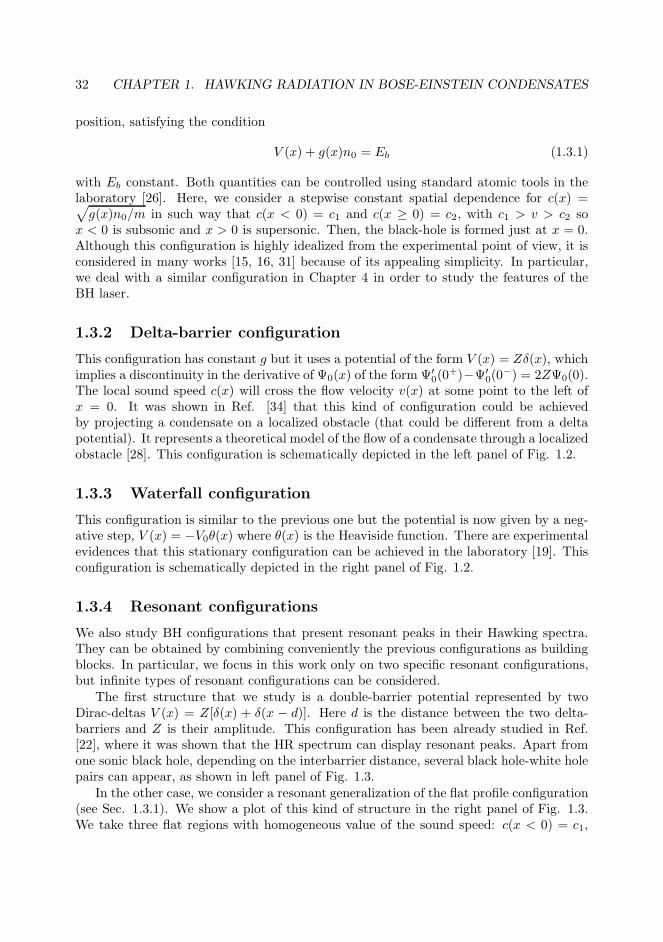
g(x)n0/m in such way that c(x < 0) = c1 and c(x ≥ 0) = c2, with c1 > v > c2 sox < 0 is subsonic and x > 0 is supersonic. Then, the black-hole is formed just at x = 0.Although this configuration is highly idealized from the experimental point of view, it isconsidered in many works [15, 16, 31] because of its appealing simplicity. In particular,we deal with a similar configuration in Chapter 4 in order to study the features of theBH laser.
1.3.2 Delta-barrier configuration
This configuration has constant g but it uses a potential of the form V (x) = Zδ(x), whichimplies a discontinuity in the derivative of Ψ0(x) of the form Ψ′
0(0+)−Ψ′
0(0−) = 2ZΨ0(0).
The local sound speed c(x) will cross the flow velocity v(x) at some point to the left ofx = 0. It was shown in Ref. [34] that this kind of configuration could be achievedby projecting a condensate on a localized obstacle (that could be different from a deltapotential). It represents a theoretical model of the flow of a condensate through a localizedobstacle [28]. This configuration is schematically depicted in the left panel of Fig. 1.2.
1.3.3 Waterfall configuration
This configuration is similar to the previous one but the potential is now given by a neg-ative step, V (x) = −V0θ(x) where θ(x) is the Heaviside function. There are experimentalevidences that this stationary configuration can be achieved in the laboratory [19]. Thisconfiguration is schematically depicted in the right panel of Fig. 1.2.
1.3.4 Resonant configurations
We also study BH configurations that present resonant peaks in their Hawking spectra.They can be obtained by combining conveniently the previous configurations as buildingblocks. In particular, we focus in this work only on two specific resonant configurations,but infinite types of resonant configurations can be considered.
The first structure that we study is a double-barrier potential represented by twoDirac-deltas V (x) = Z[δ(x) + δ(x − d)]. Here d is the distance between the two delta-barriers and Z is their amplitude. This configuration has been already studied in Ref.[22], where it was shown that the HR spectrum can display resonant peaks. Apart fromone sonic black hole, depending on the interbarrier distance, several black hole-white holepairs can appear, as shown in left panel of Fig. 1.3.
In the other case, we consider a resonant generalization of the flat profile configuration(see Sec. 1.3.1). We show a plot of this kind of structure in the right panel of Fig. 1.3.We take three flat regions with homogeneous value of the sound speed: c(x < 0) = c1,

1.3. TYPICAL BLACK-HOLE CONFIGURATIONS 33
-4 -2 0 20.0
0.5
1.0
1.5
2.0
x Ξu
ve
locityHc
uL
condensate flow
q
Hawking radiation
vHxL
cHxL
-4 -2 0 20.0
0.5
1.0
1.5
2.0
x Ξu
condensate flow
q
Hawking radiation
VHxL
vHxL
cHxL
Figure 1.2: Scheme of the delta barrier configuration described in Sec. 1.3.2 (left) andthe waterfall configuration described in Sec. 1.3.3 (right).
-2 0 2 40.0
0.5
1.0
1.5
2.0
x Ξu
velo
cityHc
uL
condensate flow
q
Hawking radiation
vHxL
cHxL
-2 0 2 40.0
0.5
1.0
1.5
2.0
x Ξu
condensate flow
q
Hawking radiation
vHxL
cHxL
Figure 1.3: Scheme of the double-barrier configuration (left) and the resonant generaliza-tion of the flat profile configuration (right), both described in Sec. 1.3.4.
c(0 ≤ x ≤ d) = c2, c(x > d) = c3, with c1 > v > c3. The middle region, with speed ofsound c2, can be chosen as subsonic or supersonic.

34 CHAPTER 1. HAWKING RADIATION IN BOSE-EINSTEIN CONDENSATES
Chapter 2Birth of a quasi-stationary black hole
in an outcoupled Bose-Einstein
condensate
2.1 Introduction
As explained at the end of the previous chapter, there are many theoretical models thatprovide an analog BH scenario in a BEC. However, they are all highly idealized from theexperimental point of view as they consider semi-infinite media and perfectly stationaryconfigurations. Moreover, they do not describe the transient regime to such BH configu-rations. On the other hand, there is a lack of experimental scenarios for BH analogs inBEC; at the present moment, the most relevant experiment was performed by the Tech-nion group [19], where a sonic black hole was created by accelerating a condensate witha negative potential. We numerically explore here an alternative realistic way to producea quasi-stationary black-hole configuration by outcoupling a large confined condensate sothat the coherent outgoing beam is dilute and fast enough to be supersonic.
The main goal of the work presented in this chapter is to explore the actual attain-ability of the steady-state regime. The hope is that spontaneous HR will be easier tomeasure in a quasi-stationary BH configuration. Within a mean-field approximation, weinvestigate the dynamics of an initially confined condensate that begins to leak as theheight of one of the confining barriers is driven from an essentially infinite to a finitevalue that permits a gentle yet appreciable flow of coherently outcoupled atoms. A simi-lar deconfinement protocol has been explored in Ref. [35]. Another theoretical proposalfor atom [34] and polariton [36] condensates is based on the idea of throwing the conden-sate onto a localized obstacle such as a potential barrier. In the present work, we focuson a finite-sized condensate and on the case where the increasingly transparent potentialis formed not by a single [23] or double [22] barrier, but by an extended optical lattice,
35
36CHAPTER 2. BIRTH OF A BLACK HOLE IN A BOSE-EINSTEIN CONDENSATE
the main reason being that the latter scenario seems more suitable for the achievement ofquasi-stationary flow within this deconfinement scheme, as will be shown later. We willsee that close-to-ideal stationary flow within the permitted energy bands is achievableunder realistic opening protocols. We also perform a preliminary study of the Hawkingradiation spectrum on top of the achieved quasi-stationary black hole. However, moreconclusive predictions about the detectability of spontaneous radiation require hardercalculations than those presented here and are left for future works.
Besides the motivation of realizing gravitational analogs, the achievement of a quasi-stationary black-hole transport scenarios is of general interest for the investigation ofatom quantum transport, in the case of both bosons [37, 38, 39, 40, 41, 42] and fermions[43, 44], within the emergent field of atomtronics [45, 46].
This chapter is arranged as follows. Section 2.2 presents the model for the gradualreduction of the optical lattice amplitude which we will be investigating. After some pre-liminary remarks in Section 2.3, the main numerical results together with some theoreticalarguments (that help to understand the observed trends) are presented in Section 2.4.The second part of that section describes the achieved quasi-stationary regime. Section2.5 addresses the more realistic case of an optical lattice having a Gaussian envelope.Interestingly, we find that the horizon lies at the maximum of the envelope and give atheoretical explanation of that fact. In Sec. 2.6 we present some preliminary results forthe Hawking spectrum above the quasi-stationary background provided by the black-holeconfiguration. The main conclusions are summarized in section 2.7. Appendix D providesa detailed description of the initial configuration of the system as it exists before the de-confinement procedure begins. Appendix E discusses the general features of Bloch wavesin the presence of nonlinearities accounting for the interaction. Finally, Appendix F.1describes the numerical method of integration and the use of absorbing boundary con-ditions, along with the method developed for integrating the resulting quasi-stationaryBdG equations.
2.2 The model
In this chapter we study the outcoupling of a one-dimensional (1D) Bose-Einstein conden-sate through a finite-size repulsive optical lattice, whose intensity is gradually lowered insuch a way that, within a finite time, the periodic barrier shifts from a regime of practicalconfinement to one of full transparency. We first focus on the mean-field dynamics, i.e.,the evolution of the condensate wave function, which obeys the following effective 1Dtime-dependent GP equation:
i~∂Ψ(x, t)
∂t=
[
− ~2
2m∂2x + V (x, t) + g|Ψ(x, t)|2
]
Ψ(x, t) , (2.2.1)
where V (x, t) is the time-dependent optical lattice potential and g the effective one-dimensional coupling constant g = 2~ωtras. The previous description is valid wheneverthe system in the 1D mean-field regime, as explained in Sec. 1.2.2. Taking the initialbulk density n0 as a typical value for the density, we can realistically set (see Sec. 2.4
2.3. PRELIMINARY REMARKS. 37
for typical values of the parameters) n0as ∼ 10−1 and n0a2tr/as ∼ 103, from which we
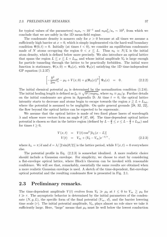
conclude that we are safely in the 1D mean-field regime.The condensate density is nonzero only for x > 0 because at all times we assume a
sufficiently high barrier at x = 0, which is simply implemented via the hard-wall boundarycondition Ψ(0, t) = 0. Initially (at times t < 0), we consider an equilibrium condensatemade of N atoms occupying the region 0 < x . L. Thus n0 ≃ N/L is the initialatom density, which is defined below more precisely. We also introduce an optical latticethat spans the region L . x . L + Llat and whose initial amplitude V0 is large enoughfor particle tunneling through the lattice to be practically forbidden. The initial wavefunction is stationary, Ψ(x, 0) = Ψ0(x), with Ψ0(x) satisfying the 1D time-independentGP equation (1.2.37)
[
− ~2
2m∂2x − µ0 + V (x, 0) + g|Ψ0(x)|2
]
Ψ0(x) = 0 . (2.2.2)
The initial chemical potential µ0 is determined by the normalization condition (1.2.6).The initial healing length is defined as ξ0 ≡
√
~2/mgn0, where n0 ≡ µ0/g. Further detailson the initial condensate are given in Appendix D. At time t = 0, the optical latticeintensity starts to decrease and atoms begin to escape towards the region x & L + Llat,where the potential is assumed to be negligible. On quite general grounds [28, 32, 22],the flow beyond the optical lattice can be expected to be supersonic.
We assume that the optical lattice is made of two fixed phase lasers of wavelengthλ and whose wave vectors form an angle θ [47, 48]. The time-dependent optical latticepotential is chosen so that in the lattice region (defined by L− d
2 ≤ x ≤ L− d2 +Llat) and
for times t ≥ 0,
V (x, t) = V (t) cos2 [kL(x− L)]
V (t) = V∞ + (V0 − V∞)e−t/τ , (2.2.3)
where kL = π/d and d = λ/ [2 sin(θ/2)] is the lattice period, while V (x, t) = 0 everywhereelse.
The potential profile in Eq. (2.2.3) is somewhat idealized. A more realistic choiceshould include a Gaussian envelope. For simplicity, we choose to start by consideringa flat-envelope optical lattice, where Bloch’s theorem can be invoked with reasonableconfidence. We will see that, remarkably, essentially the same results are obtained whena more realistic Gaussian envelope is used. A sketch of the time-dependent, flat-envelopeoptical potential and the resulting condensate flow is presented in Fig. 2.1.
2.3 Preliminary remarks.
The time-dependent amplitude V (t) evolves from V0 ≫ µ0 at t ≤ 0 to V∞ & µ0 fort ≫ τ . The asymptotic behavior is determined by the initial parameters of the conden-sate (N, g, L), the specific form of the final potential (V∞, d), and the barrier loweringtime scale (τ). The initial potential amplitude, V0, plays almost no role since we take itsufficiently large. Here, “large” means that µ0 must lie well below the lowest conduction

38CHAPTER 2. BIRTH OF A BLACK HOLE IN A BOSE-EINSTEIN CONDENSATE
Figure 2.1: Schematic representation of the emitting condensate setup here studied.Within the ideal lattice scenario, hard-wall boundary conditions are assumed at x = 0 andan optical lattice lies in the region L < x < Llat with a time-dependent amplitude suchthat the potential V (x, t) (represented by the semi-transparent yellow surface over thex− t plane) evolves from strongly to moderately confining. The resulting time-dependentdensity profile n(x, t) is represented by the grey-blue surface. The vertical axis repre-sents the density. The surface V (x, t) is uplifted to provide a better vision of n(x, t).Some parameters defined in the main text are indicated. The trend towards a long-timequasi-stationary flow regime can be qualitatively observed.
band of the initial optical lattice potential in order to have an effectively confined con-densate. On the other hand, the properties of the final steady state are insensitive to τunless τ is very small (see Subsection 2.4.1).
The main goal of the present work is to identify the barrier-lowering protocol thatbest leads to the formation of a quasi-stationary outcoupled black-hole configuration, bywhich we mean a black-hole flow regime characterized by parameters that vary slowly intime in a sense that will be specified later. As to the space dependence in that regime,we require the density to be as uniform as possible in the upstream region 0 < x . L. Inthe supersonic downstream region (x & L + Llat) we also want an uniform flow profile,even though this will be more difficult to achieve due to the small density. On the otherhand, in the optical lattice region, the flow should be as close as possible to that of apropagating Bloch wave. At the boundary between these two regions, large gradients
2.4. IDEAL OPTICAL LATTICE 39
of the flow speed and density are likely to occur, but the current density should remainessentially uniform.
Throughout this chapter, when we talk about bands, we will be referring to theSchrodinger (non-interacting) bands, unless specified otherwise. Bands in a nonlinearcontext are discussed in Appendix E. We will see that, in virtually all cases, the relevantproperties of the optical lattice are determined by its lowest band since the number ofwells of the lattice is sufficiently large. An important result is that, due to the finite size ofthe subsonic reservoir, the quasi-stationary flow is formed when the space-averaged chem-ical potential lies slightly above the bottom of the lowest lattice band. This implies that,once in the quasi-stationary regime, the interacting term (and consequently the density)has to be small almost everywhere in the optical lattice region g|Ψ(x, t)|2 ≪ (~kL)
2/m;see Appendix E for details. In the non-interacting regime, Eq. (2.2.1) becomes the usualSchrodinger equation, which for a sinusoidal potential can be transformed into Mathieu’sequation [49], whose solutions and band structure are well known.
The asymptotic band structure can be characterized by the dimensionless parameter
v ≡ mV∞/8~2k2L . (2.3.1)
The nearly-free atom regime occurs when v ≪ 1. Then bands are wide while gaps arenarrow. By contrast, in the tight-binding regime (v ≫ 1), bands are narrow and widelyspaced. Since v ∝ V∞d2, the band structure can be modified by changing the latticeamplitude or its spacing.
2.4 Ideal optical lattice
In this work, the unit length is the initial bulk healing length ξ0 defined in Section 2.2.Accordingly, velocities are measured in units of the sound speed, c0 ≡
√
gn0/m, andtimes in units of t0 ≡ ξ0/c0. Energies are expressed in units of the initial chemicalpotential µ0 = mc20. We consider quasi–one-dimensional condensates of 87Rb, which aretypically made of N ∼ 104 − 107 atoms and have mass m = 1.44 × 10⁻²⁵ kg. Thetypical order of magnitude of the transverse trapping frequency is ωtr ∼ 2π × 10 − 103
Hz and the confinement length varies in the range L ∼ 10 − 400µm. The scatteringlength satisfies as ∼ 100a0 = 5.29 nm, with a0 = 5.29 × 10⁻¹¹ m the Bohr radius. Theoptical lattice periodicity is bounded from below, d > λ/2, for geometrical reasons [seebelow Eq. (2.2.3)]. The value of λ is chosen to be sufficiently far from the resonanceto avoid any spontaneous emission and on the blue-side of the resonance to produce arepulsive potential (λ < 780 nm for rubidium atoms). The simulations are run up to timest ∼ 104 − 105t0. As t0 = (2n0asωtr)
−1 ∼ 10−4 s, then t ∼ 1 − 10 s for our simulations,which is on the order of the mean lifetime of this type of condensates. Although we focuson the usual case of 87Rb, the results of the simulations here presented can be extendedto arbitrary atoms.
In the simulations we use a numerical scheme based on the Crank-Nicolson methodto integrate the time-dependent GP equation (2.2.1). Hard wall boundary conditions areassumed at x = 0. At the other end of the finite size computational grid (located atx = Lg, with Lg the total length of the grid), we use absorbing boundary conditions. Lg
40CHAPTER 2. BIRTH OF A BLACK HOLE IN A BOSE-EINSTEIN CONDENSATE
is taken so that the final point of the grid is sufficiently far from the end of the opticallattice for the supersonic region to be clearly observed. Further details on numericalmethods are given in Appendix F.
2.4.1 Analysis of the simulations
To characterize the quasi-stationary regime, we define the local chemical potential as
µ(x, t) ≡ − ~2
2m
∂2Ψ(x, t)/∂x2
Ψ(x, t)+ V (x, t) + g|Ψ(x, t)|2 , (2.4.1)
which, we note, can be complex. For a stationary solution, Ψ(x, t) = e−iµt/~Ψ0(x), onehas µ(x, t) = µ, real and independent of (x, t). The one-dimensional current, obtainedfrom Eq.(1.2.23):
J(x, t) = − i~
2m
(
Ψ∗(x, t)∂Ψ(x, t)
∂x−Ψ(x, t)
∂Ψ∗(x, t)
∂x
)
(2.4.2)
is also independent of (x, t) for a one dimensional stationary solution, as dictated by theone dimensional version of the continuity equation (1.2.25) [see also Eq. (A.0.1) andrelated discussion]. In the quasi-stationary regime the uniformity of J(x, t) is impossibleto fulfill strictly, because the current is zero at x = 0 while the emitted atoms carry anonzero current. Thus, there must be a current gradient and, by the continuity equation,the density has to be time dependent. The hope is however that, in the quasi-stationaryregime, the condensate leak is sufficiently slow for the time dependence to be weak.
On the other hand, we can expect that, in the quasi-stationary regime, µ(x, t) isa sufficiently uniform function, with small spatial variations around its space-averagedmean value. To check this expectation in a quantitative manner, we introduce the space-averaged chemical potential µ(t) together with an appropriate measure of its relativespatial fluctuations σ(t):
µ(t) ≡∫ Lg
0 dxn(x, t)µ(x, t)∫ Lg
0dxn(x, t)
σ(t) ≡ 1
µ(t)
[
∫ Lg
0 dxn(x, t)|µ(x, t) − µ(t)|2∫ Lg
0 dxn(x, t)
]12
. (2.4.3)
We recall that µ(x, t) and µ(t) can be complex. A nonzero imaginary part of µ(x, t)reflects a leaking condensate, as revealed by the local relation
∂n
∂t=
2
~n Imµ . (2.4.4)
Accordingly, we can define and compute the emission rate per particle as
Γ(t) ≡ j(Lg, t)∫ Lg
0 dx n(x, t)= − 2
~Im µ(t) , (2.4.5)

2.4. IDEAL OPTICAL LATTICE 41
where the continuity equation has been used. The spatial average of the time-dependentchemical potential, Eq. (2.4.3), is mostly determined by the subsonic region, whereµ(x, t) ≃ gn(x, t).
By rescaling the condensate wave function as Ψ(x, t) → √n0Ψ(x, t), we observe clearly
the actual degrees of freedom of the system. Given the initial healing length, ξ0, onlyL/ξ0, d/ξ0, τ/t0, V∞/mc20 and nosc ≡ Llat/d (number of oscillations in the optical lattice)are free parameters of the problem (we have already noted that V0 plays almost no rolein the confinement limit V0 ≫ µ0).
We find that, for the pertinent experimental ranges, namely, L ∼ 10− 400µm, varia-tions of L/ξ0 have little effect on the properties of the quasi-stationary regime. Specifically,they have a small influence on the time needed to achieve the desired quasi-stationarity,which grows weakly with the initial size of the condensate as a larger confined condensateneeds more time to empty.
A similar point can be made about nosc, which becomes unimportant when it lies inthe range nosc ∼ 10 − 100. The (relatively small) effect of increasing nosc even furtheris that there are more spatial fluctuations in the chemical potential, for two reasons: (a)there are more spatial fluctuations of µ(x, t) because of multiple atomic reflections acrossthe wells, an effect that is enhanced for larger optical lattices; (b) the larger the lattice,the bigger its contribution to the average chemical potential and its fluctuations.
In summary, except for the above remarks, only the parameters d/ξ0, V∞/mc20 andτ/t0, have a noticeable effect on the transport properties of the system. We proceed tostudy their role on the results of the simulations.
Role of the final band structure
As noted before, the combination of d and V∞ fixes the final band structure. Figure2.2 shows the various scenarios which one may find depending on the long-time widthand position of the lowest band with respect to the initial chemical potential, µ0. Theband structure is computed numerically. The desired steadiness of the long time behaviorimproves with the width of the band, as the first row in Fig. 2.2 reveals. In Fig. 2.2a,a favorable case with a wide band is presented and compared with a less favorable casein Fig. 2.2b, which has the same conduction band minimum but a narrower conductionband. After a short transient, a comparison of the relative chemical-potential standarddeviation σ(t), as defined in Eq. (2.4.3) and plotted in this graph, shows a clear advantagein the use of wider bands. For instance, in Fig. 2.2a, σ(t) ∼ 10−4 in the stationary (longtime) regime, about 10 times smaller than in Fig. 2.2b.
Besides, after a transition time of order ∼ 5000t0, all the characteristic magnitudes ofthe system shown in Fig. 2.2a vary slowly enough in time to properly view the resultingflow regime as quasi-stationary. In fact, the leak is so slow that other processes whichlimit the lifetime of the condensate (such as condensate decay due to inelastic collisions)operate on a shorter time scale.
If the chemical potential reaches and goes below the bottom of the conducting band ina relatively short time, then a transition occurs to an essentially confined situation wherethe leaking is exponentially small, corresponding to an atom transmission probabilityT (Llat) ∝ exp(−κLlat), where κ ∝ √
Emin − µ, with Emin the bottom of the conducting

42CHAPTER 2. BIRTH OF A BLACK HOLE IN A BOSE-EINSTEIN CONDENSATE
0.5
1
1.5
2
Re
µ(t
)/m
c2 0 V∞ = 2 mc2
0
d = 1.89 ξ0
(a) (b)V∞ = 2.324 mc2
0
d = 2.83 ξ0
0.02
0.04
0.06
0.08
σ(t
)
1 2 3
0.5
1
1.5
2
t (104t0)
Re
µ(t
)/m
c2 0 V∞ = 2 mc2
0
d = 2.84 ξ0
(c)
1 2 3 1 2 3
t (104t0)
(d)V∞ = mc2
0
d = 2.84 ξ0
1 2 3
0.02
0.04
0.06
0.08
σ(t
)
Figure 2.2: Time evolution of the real part of the space-averaged chemical potential µ(t)(black dashed) and its fluctuation spread σ(t) (green solid), both defined in Eq. (2.4.3).The gap and conduction band of the instantaneous band structure [computed from thepotential Eq. (2.2.3)] are indicated, respectively, by grey and white backgrounds. Allgraphs are computed with τ = 500 t0, L = 400µm, nosc = 30, N = 104, and ωtr = 2π ×4 kHz, which yields n0 = 25µm−1 and ξ0 = 0.3175µm. The long-time potential amplitudeV∞ and the lattice spacing d are indicated in the graphs. The dimensionless parameter v[see Eq. (2.3.1)] takes the values (0.0905, 0.2350, 0.2036, 0.1018) for graphs (a)-(d). Thesetups (a) and (b) are designed to have the same band bottom. The simulations are rununtil a time 4 × 10⁴ t0 = 5.5 s. Note that the scale of σ(t) is considerably enlarged. Theinitial value σ(0) (only observed with some magnification) is spurious, and is related tothe discrete approximation to the derivatives in Eq. (2.4.1).
band. This situation whereby one soon reaches the regime µ < Emin is not interesting forour purposes because we need some appreciable flux in order to form a useful black-holeconfiguration. As a consequence, we typically consider condensates so large that the timeneeded to reach the bottom of the conduction band is longer than the typical lifetime ofthe condensate.
A further argument can be invoked in favor of wide bands. In virtually all the cases wehave addressed, Re µ(t) drops until it almost reaches the bottom of the conduction band,where leaking is slow. In the resulting regime, the density in the lattice is very small,

2.4. IDEAL OPTICAL LATTICE 43
gnr ≪ ~2k2L/m, where nr is the mean density in the optical lattice, as defined precisely insubsection 2.4.2. It is shown in Appendix E that, in this regime of low interactions, thewidth of the conduction band for the linear perturbations (whose evolution is governed bythe BdG equations) is very close to that obtained for the linear Schrodinger equation, andthe corrections are there computed. This means that the optical lattice acts like a low-pass filter, the band width being the equivalent of the cutoff frequency. The higher thecutoff, the wider is the transmission band of the lattice. As a consequence, fluctuationson the subsonic side are transmitted away through the optical lattice, which reduces thespace fluctuations in the chemical potential.
Another interesting trend can be observed in the second row of Fig. 2.2. When placingµ0 slightly below the top of the conduction band or in the first gap, as Fig. 2.2d illustrates,the leaking occurs faster but the reached regime presents much larger fluctuations than inthe other cases shown in Fig. 2.2. For the purpose of keeping σ(t) ≪ 1, a more favorablesituation for the chemical potential is shown in Fig. 2.2c. There, for the same length d asin Fig. 2.2d but a higher barrier amplitude V∞, the chemical potential is initially placedin the final conduction band. This case clearly yields smaller fluctuations, even thoughthe width of the conduction band is smaller. This shows that, besides having wide bands,one also needs that µ0 be placed close to the bottom of the final conduction band in orderto obtain a more favorable quasi-stationary regime. We discuss this feature in more detailin Sec. (2.4.2).
Within the nearly-free particle approximation (v ≪ 1), the bottom and top of the firstconduction band are given by the relations:
Emin(v) = 8ER(v − v2 +O(v4))
Emax(v) = ER(1 + 4v − 2v2 +O(v4)) , (2.4.6)
where ER ≡ ~2k2L/2m is the recoil energy of the optical lattice. Given that kL = π/d, the
condition that the initial chemical potential lies within the final conduction band, i.e.,
Emin(v) < µ0 < Emax(v) , (2.4.7)
is guaranteed to be satisfied if8ERv < µ0 < ER . (2.4.8)
The left inequality is justV∞2
< µ0 , (2.4.9)
while the right inequality can be rewritten as:
d <π√2ξ0 . (2.4.10)
Equations (2.4.9), (2.4.10) express a sufficient condition to satisfy Eq. (2.4.7).
Non-adiabatic effects
In the favorable situation shown in Fig. 2.2a, the dependence on τ is not important aslong as τ ≫ t0. A simulation is presented in Fig. 2.3 which shows that, in the fast regime

44CHAPTER 2. BIRTH OF A BLACK HOLE IN A BOSE-EINSTEIN CONDENSATE
1 2 3
0.5
1
1.5
2
t (104t0)
Re
µ(t
)/m
c2 0
1 2 3
0.02
0.04
0.06
0.08
σ(t
)
Figure 2.3: Fast barrier lowering. Same parameters as in Fig. 2.2a except for τ = t0,which is very small to be observed on this scale.
τ ∼ t0, and due to the high-frequency excitations induced by the short lowering timescale, σ(t) remains higher than in the adiabatic case of Fig. 2.2a, corresponding to asimulation with the same parameters but with τ ≫ t0.
2.4.2 Quasi-stationary regime
From the discussion in the previous subsection (2.4.1), and particularly through the sit-uation shown in Fig. 2.2a, we have learned that, in a setup with typical experimentalvalues and that presents wide bands, initial chemical potential close to the bottom of thefinal conduction band and adiabatic evolution (τ ≫ t0), the system evolves towards aquasi-stationary regime in times shorter than the typical lifetime of a condensate.
The quasi-stationary regime can be defined as that in which Reµ(x, t) is essentiallyuniform [σ(t) ≪ 1] and its global time variations take place on a time scale of the order ofor greater than the condensate lifetime. We focus our study on the most favorable quasi-stationary scenarios, which here we identify with those satisfying σ(t) ∼ 10−3 − 10−4.
The achievement of this regime is of general interest as a scenario for the study ofatom quantum transport since it provides a quasi-stationary supersonic current. Related
2.4. IDEAL OPTICAL LATTICE 45
directly to the main topic of this work, one may expect spontaneous Hawking radiationto be detectable above a quasi-stationary background with small spatial fluctuations.
In the present section we discuss several features of the condensate wave function forthe quasi-stationary regime. For illustrative purposes, all the graphs considered in thissubsection have been obtained for a system with the parameters of Fig. 2.2a, which aresufficiently representative.
We can extend the concept of local sound and flow velocities to time-dependent situ-ations [see Chapter 1 for the notation]:
v(x, t) ≡ ~∂xθ(x, t)
m,
c(x, t) ≡√
gn(x, t)
m, (2.4.11)
The spatial variations of both velocities are small in the subsonic and supersonic regions,but not in the lattice, where we note that c(x, t) must not be regarded as the actual latticesound speed; see Appendix E for the computation of the actual sound speed.
The profile of both quantities computed at a time t = 4 × 10⁴ t0 for the simulationof Fig. 2.2a is shown in Fig. 2.4. The subsonic zone shows an essentially flat (uniform)density and flow speed profile in the sense that the spatial fluctuations are on the orderof ∼ 10−4n0 for the density and ∼ 10−3c0 for the flow speed, too small to be observed inFig. 2.4. In Appendix D, we give an approximate analytical formula [Eq. (D.1.21)] forthe wave function of the confined condensate which fits the numerical results within thislevel of accuracy, but replacing ξ0 by the healing length defined by the quasi-stationaryvalue of the subsonic density gnu ≃ µ ≃ Emin. This good agreement reflects the low valueof the flow velocity in the upstream region.
On the other hand, in the deep central region of the optical lattice, Bloch’s theoremis satisfied. We introduce the space-averaged density nr(t) by averaging n(x, t) over theoptical lattice after excluding 10 lattice sites at each end of the lattice. That averagedensity, combined with the optical lattice parameters, yields an effective sound velocity[see Eq. (E.2.15)] that is plotted as a horizontal green segment spanning the averagedregion in Fig. 2.4. It can be clearly seen that, within the bulk of the optical lattice, theflow is subsonic, with the horizon on its right edge. In the quasi-stationary regime, nr(t)decreases at a rate comparable to the inverse lifetime of the condensate, as the inset inFig. 2.5 shows.
A check on the approximate validity of Bloch’s theorem in the presence of non-linearcorrections, for the central part of the optical lattice and in the quasi-stationary regime,is also shown in Fig. 2.5. In this graph, the real part of µ(t) is compared with the time-dependent chemical potential computed using nr(t) and assuming zero Bloch momentum,as explained in the first paragraphs of Appendix E. The good agreement between the twocurves suggests that the condensate is flowing with very small Bloch momentum.
At the boundaries of the optical lattice there are strong variations of the density dueto the the matching between the vastly different densities found on both the subsonic andthe supersonic sides.
Downstream, once in the quasi-stationary regime, both density and flow speed profilesare almost uniform. This is hinted at in Fig. 2.4 but not shown explicitly. Indeed, part of
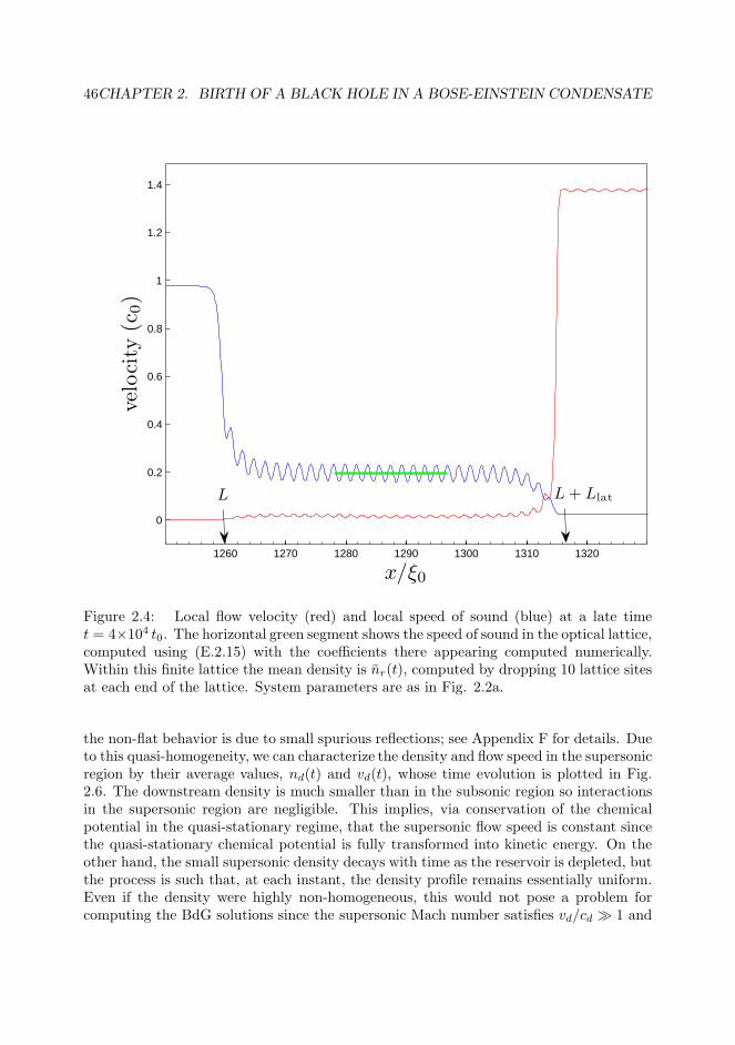
46CHAPTER 2. BIRTH OF A BLACK HOLE IN A BOSE-EINSTEIN CONDENSATE
1260 1270 1280 1290 1300 1310 1320
0
0.2
0.4
0.6
0.8
1
1.2
1.4
x/ξ0
velo
city
(c0)
L + LlatL
Figure 2.4: Local flow velocity (red) and local speed of sound (blue) at a late timet = 4×10⁴ t0. The horizontal green segment shows the speed of sound in the optical lattice,computed using (E.2.15) with the coefficients there appearing computed numerically.Within this finite lattice the mean density is nr(t), computed by dropping 10 lattice sitesat each end of the lattice. System parameters are as in Fig. 2.2a.
the non-flat behavior is due to small spurious reflections; see Appendix F for details. Dueto this quasi-homogeneity, we can characterize the density and flow speed in the supersonicregion by their average values, nd(t) and vd(t), whose time evolution is plotted in Fig.2.6. The downstream density is much smaller than in the subsonic region so interactionsin the supersonic region are negligible. This implies, via conservation of the chemicalpotential in the quasi-stationary regime, that the supersonic flow speed is constant sincethe quasi-stationary chemical potential is fully transformed into kinetic energy. On theother hand, the small supersonic density decays with time as the reservoir is depleted, butthe process is such that, at each instant, the density profile remains essentially uniform.Even if the density were highly non-homogeneous, this would not pose a problem forcomputing the BdG solutions since the supersonic Mach number satisfies vd/cd ≫ 1 and
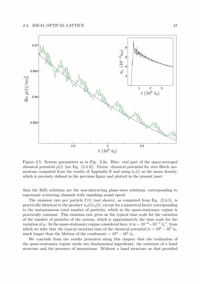
2.4. IDEAL OPTICAL LATTICE 47
2.5 3 3.5
0.955
0.96
0.965
0.97
t (104 t0)
Re
µ(t
)/m
c2 0
1 2 3
2
4
6
8
t (104 t0)
nr
(10−
2n
0)
Figure 2.5: System parameters as in Fig. 2.2a. Blue: real part of the space-averagedchemical potential µ(t) [see Eq. (2.4.3)]. Green: chemical potential for zero Bloch mo-mentum computed from the results of Appendix E and using nr(t) as the mean density,which is precisely defined in the previous figure and plotted in the present inset.
then the BdG solutions are the non-interacting plane-wave solutions, corresponding tosupersonic scattering channels with vanishing sound speed.
The emission rate per particle Γ(t) (not shown), as computed from Eq. (2.4.5), ispractically identical to the product nd(t)vd(t), except for a numerical factor correspondingto the instantaneous total number of particles, which in the quasi-stationary regime ispractically constant. This emission rate gives us the typical time scale for the variationof the number of particles of the system, which is approximately the time scale for thevariation of µ. In the quasi-stationary regime considered here, it is∼ 10−6−10−7 t−1
0 , fromwhich we infer that the typical variation time of the chemical potential is ∼ 106 − 107 t0,much longer than the lifetime of the condensate ∼ 104 − 105 t0.
We conclude from the results presented along this chapter that the realization ofthe quasi-stationary regime needs two fundamental ingredients: the existence of a bandstructure and the presence of interactions. Without a band structure as that provided

48CHAPTER 2. BIRTH OF A BLACK HOLE IN A BOSE-EINSTEIN CONDENSATE
1 2 3
−5
0
5
t (104 t0)
v d(c
0)
1 2 3
1
2
3
nd(1
0−
3n
0)
Figure 2.6: Time evolution of the mean density and the mean flow velocity on the super-sonic side. The averages are taken in the sense of integrals along the downstream regionwhere the profile is essentially flat. System parameters are as in Fig. 2.2a.
by the optical lattice, the condensate would continue leaking through the barrier at afast rate. On the other hand, the presence of interactions (as reflected in the fact that∂µ/∂n 6= 0) allows the condensate to stabilize its flow near the bottom of the conductionband. If the interactions in the subsonic region were negligible, the condensate wouldempty quickly (if µ0 lied in the final conducting band) or it would remain confined (if µ0
lied in the final gap).
We have produced some movies to observe such trends, where we consider simulationswith the same parameters of Fig. 2.2a but now L = 10µm and N = 250. The qualitativeconclusions are similar. In Video 1, we see the time evolution of the density of a conden-sate confined by an ideal optical lattice of 30 barriers. We see that the system achievesthe desired quasi-stationary regime. On the other hand, in Video 2, we introduce thesame potential but with just a single barrier, i.e., nosc = 1. We observe that the fluidleaks faster through the single barrier because the potential does not provide a conduc-tion band that effectively reduces the leaking of the reservoir. This conclusion applies
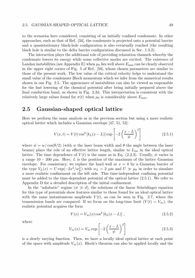
2.5. GAUSSIAN-SHAPED OPTICAL LATTICE 49
to the scenarios here considered, consisting of an initially confined condensate. In otherapproaches, such as that of Ref. [34], the condensate is projected onto a potential barrierand a quasistationary black-hole configuration is also eventually reached (the resultingblack hole is similar to the delta barrier configuration discussed in Sec. 1.3.2).
The interaction plays the additional role of providing relaxation channels whereby thecondensate lowers its energy while some collective modes are excited. The existence ofLandau instabilities (see Appendix E) when µ0 lies well aboveEmin can be clearly observedin the upper right corner of Fig. 5 of Ref. [50], whose chosen parameters are similar tothose of the present work. The low value of the critical velocity helps to understand thesmall value of the condensate Bloch momentum which we infer from the numerical resultsshown in our Fig. 2.5. The appearance of instabilities can also be viewed as responsiblefor the fast lowering of the chemical potential after being initially prepared above thefinal conduction band, as shown in Fig. 2.2d. This interpretation is consistent with therelatively large values found for σ(t) when µ0 is considerably above Emin.
2.5 Gaussian-shaped optical lattice
Here we perform the same analysis as in the previous section but using a more realisticoptical lattice which includes a Gaussian envelope [47, 51, 52]:
V (x, t) = V (t) cos2 [kL(x− L)] exp
[
−2
(
x− L
w
)2]
(2.5.1)
where w = w/ cos(θ/2) (with w the laser beam width and θ the angle between the laserbeams) plays the role of an effective lattice length, similar to Llat in the ideal opticallattice. The time dependence of V (t) is the same as in Eq. (2.2.3). Usually, w varies ina range 10 − 200 µm. Here, L is the position of the maximum of the lattice Gaussianenvelope. For consistency, we replace the hard wall at x = 0 by a Gaussian barrier ofthe type VL(x) = U exp(−2x2/w2
L) with wL = 2 µm and U ≫ µ0 in order to simulatea more realistic confinement on the left side. This time-independent confining potentialmust be added to the time-dependent potential of the optical lattice (2.5.1). We refer toAppendix D for a detailed description of the initial confinement.
In the “adiabatic” regime (w ≫ d), the solutions of the linear Schrodinger equationfor this type of potentials show features similar to those found for an ideal optical latticewith the same instantaneous amplitude V (t), as can be seen in Fig. 2.7, where thetransmission bands are compared. If we focus on the long-time limit (V (t) = V∞), therealistic potential acquires the form
V (x) = V∞(x) cos2 [kL(x− L)] , (2.5.2)
where
V∞(x) = V∞ exp
[
−2
(
x− L
w
)2]
(2.5.3)
is a slowly varying function. Then, we have a locally ideal optical lattice at each pointof the space with amplitude V∞(x). Bloch’s theorem can also be applied locally and the
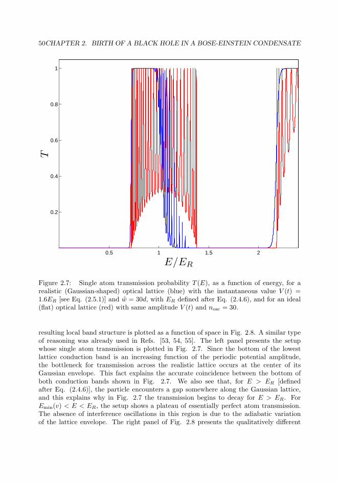
50CHAPTER 2. BIRTH OF A BLACK HOLE IN A BOSE-EINSTEIN CONDENSATE
0.5 1 1.5 2
0.2
0.4
0.6
0.8
1
E/ER
T
Figure 2.7: Single atom transmission probability T (E), as a function of energy, for arealistic (Gaussian-shaped) optical lattice (blue) with the instantaneous value V (t) =1.6ER [see Eq. (2.5.1)] and w = 30d, with ER defined after Eq. (2.4.6), and for an ideal(flat) optical lattice (red) with same amplitude V (t) and nosc = 30.
resulting local band structure is plotted as a function of space in Fig. 2.8. A similar typeof reasoning was already used in Refs. [53, 54, 55]. The left panel presents the setupwhose single atom transmission is plotted in Fig. 2.7. Since the bottom of the lowestlattice conduction band is an increasing function of the periodic potential amplitude,the bottleneck for transmission across the realistic lattice occurs at the center of itsGaussian envelope. This fact explains the accurate coincidence between the bottom ofboth conduction bands shown in Fig. 2.7. We also see that, for E > ER [definedafter Eq. (2.4.6)], the particle encounters a gap somewhere along the Gaussian lattice,and this explains why in Fig. 2.7 the transmission begins to decay for E > ER. ForEmin(v) < E < ER, the setup shows a plateau of essentially perfect atom transmission.The absence of interference oscillations in this region is due to the adiabatic variationof the lattice envelope. The right panel of Fig. 2.8 presents the qualitatively different
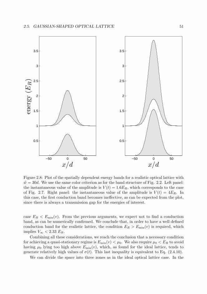
2.5. GAUSSIAN-SHAPED OPTICAL LATTICE 51
x/d
ener
gy(E
R)
−50 0 50
0.5
1
1.5
2
2.5
3
3.5
x/d−50 0 50
0.5
1
1.5
2
2.5
3
3.5
Figure 2.8: Plot of the spatially dependent energy bands for a realistic optical lattice withw = 30d. We use the same color criterion as for the band structure of Fig. 2.2. Left panel:the instantaneous value of the amplitude is V (t) = 1.6ER, which corresponds to the caseof Fig. 2.7. Right panel: the instantaneous value of the amplitude is V (t) = 4ER. Inthis case, the first conduction band becomes ineffective, as can be expected from the plot,since there is always a transmission gap for the energies of interest.
case ER < Emin(v). From the previous arguments, we expect not to find a conductionband, as can be numerically confirmed. We conclude that, in order to have a well definedconduction band for the realistic lattice, the condition ER > Emin(v) is required, whichimplies V∞ < 2.33 ER.
Combining all these considerations, we reach the conclusion that a necessary conditionfor achieving a quasi-stationary regime is Emin(v) < µ0. We also require µ0 < ER to avoidhaving µ0 lying too high above Emin(v), which, as found for the ideal lattice, tends togenerate relatively high values of σ(t). This last inequality is equivalent to Eq. (2.4.10).
We can divide the space into three zones as in the ideal optical lattice case. In the
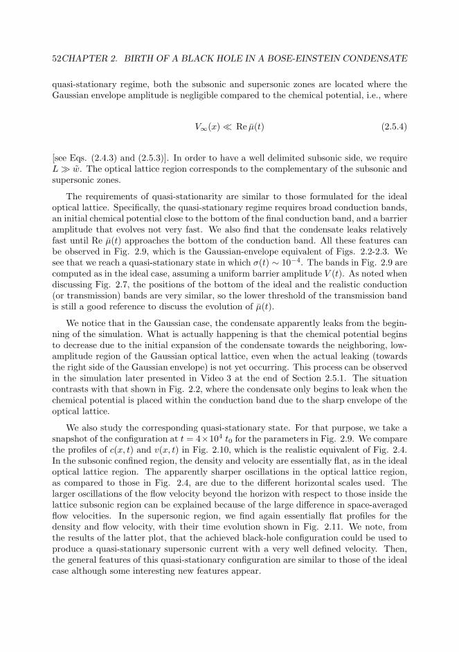
52CHAPTER 2. BIRTH OF A BLACK HOLE IN A BOSE-EINSTEIN CONDENSATE
quasi-stationary regime, both the subsonic and supersonic zones are located where theGaussian envelope amplitude is negligible compared to the chemical potential, i.e., where
V∞(x) ≪ Re µ(t) (2.5.4)
[see Eqs. (2.4.3) and (2.5.3)]. In order to have a well delimited subsonic side, we requireL≫ w. The optical lattice region corresponds to the complementary of the subsonic andsupersonic zones.
The requirements of quasi-stationarity are similar to those formulated for the idealoptical lattice. Specifically, the quasi-stationary regime requires broad conduction bands,an initial chemical potential close to the bottom of the final conduction band, and a barrieramplitude that evolves not very fast. We also find that the condensate leaks relativelyfast until Re µ(t) approaches the bottom of the conduction band. All these features canbe observed in Fig. 2.9, which is the Gaussian-envelope equivalent of Figs. 2.2-2.3. Wesee that we reach a quasi-stationary state in which σ(t) ∼ 10−4. The bands in Fig. 2.9 arecomputed as in the ideal case, assuming a uniform barrier amplitude V (t). As noted whendiscussing Fig. 2.7, the positions of the bottom of the ideal and the realistic conduction(or transmission) bands are very similar, so the lower threshold of the transmission bandis still a good reference to discuss the evolution of µ(t).
We notice that in the Gaussian case, the condensate apparently leaks from the begin-ning of the simulation. What is actually happening is that the chemical potential beginsto decrease due to the initial expansion of the condensate towards the neighboring, low-amplitude region of the Gaussian optical lattice, even when the actual leaking (towardsthe right side of the Gaussian envelope) is not yet occurring. This process can be observedin the simulation later presented in Video 3 at the end of Section 2.5.1. The situationcontrasts with that shown in Fig. 2.2, where the condensate only begins to leak when thechemical potential is placed within the conduction band due to the sharp envelope of theoptical lattice.
We also study the corresponding quasi-stationary state. For that purpose, we take asnapshot of the configuration at t = 4×10⁴ t0 for the parameters in Fig. 2.9. We comparethe profiles of c(x, t) and v(x, t) in Fig. 2.10, which is the realistic equivalent of Fig. 2.4.In the subsonic confined region, the density and velocity are essentially flat, as in the idealoptical lattice region. The apparently sharper oscillations in the optical lattice region,as compared to those in Fig. 2.4, are due to the different horizontal scales used. Thelarger oscillations of the flow velocity beyond the horizon with respect to those inside thelattice subsonic region can be explained because of the large difference in space-averagedflow velocities. In the supersonic region, we find again essentially flat profiles for thedensity and flow velocity, with their time evolution shown in Fig. 2.11. We note, fromthe results of the latter plot, that the achieved black-hole configuration could be used toproduce a quasi-stationary supersonic current with a very well defined velocity. Then,the general features of this quasi-stationary configuration are similar to those of the idealcase although some interesting new features appear.
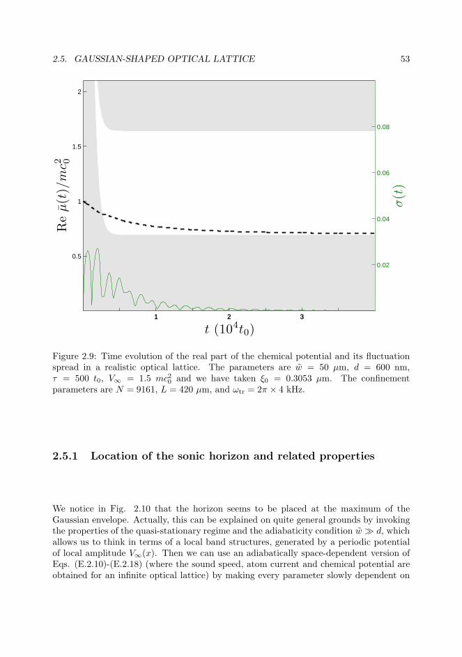
2.5. GAUSSIAN-SHAPED OPTICAL LATTICE 53
1 2 3
0.5
1
1.5
2
t (104t0)
Re
µ(t
)/m
c2 0
1 2 3
0.02
0.04
0.06
0.08
σ(t
)
Figure 2.9: Time evolution of the real part of the chemical potential and its fluctuationspread in a realistic optical lattice. The parameters are w = 50 µm, d = 600 nm,τ = 500 t0, V∞ = 1.5 mc20 and we have taken ξ0 = 0.3053 µm. The confinementparameters are N = 9161, L = 420 µm, and ωtr = 2π × 4 kHz.
2.5.1 Location of the sonic horizon and related properties
We notice in Fig. 2.10 that the horizon seems to be placed at the maximum of theGaussian envelope. Actually, this can be explained on quite general grounds by invokingthe properties of the quasi-stationary regime and the adiabaticity condition w ≫ d, whichallows us to think in terms of a local band structures, generated by a periodic potentialof local amplitude V∞(x). Then we can use an adiabatically space-dependent version ofEqs. (E.2.10)-(E.2.18) (where the sound speed, atom current and chemical potential areobtained for an infinite optical lattice) by making every parameter slowly dependent on

54CHAPTER 2. BIRTH OF A BLACK HOLE IN A BOSE-EINSTEIN CONDENSATE
1150 1200 1250 1300 1350 1400 1450 1500 1550 1600
0
0.2
0.4
0.6
0.8
1
1.2
1.4
x/ξ0
velo
city
(c0)
L
Figure 2.10: Local flow velocity (red) and local speed of sound (blue) at t = 4 × 10⁴ t0.System parameters are as in Fig. 2.9.
x. In particular, we take:
s(x) =
[
gnr(x)
m∗(x)α(1)0 (x)
]12
j(x) ≃ nr(x)v(x) (2.5.5)
µ(x) ≃ Emin(x) +1
2m∗(x)v2(x) +m∗(x)s2(x) ,
where we neglect the time dependence because the system is assumed to be already inthe quasi-stationary regime. The local averages for nr, v are taken over several latticeperiods. In the quasi-stationary regime, the chemical potential is already close to thebottom of the conduction band, so the perturbative treatment considered in AppendixE is valid. By taking spatial derivatives (denoted by ′) while noting that the chemicalpotential is almost uniform, µ(x) ≃ µ, and that ∂xj(x) can be neglected (as implied by
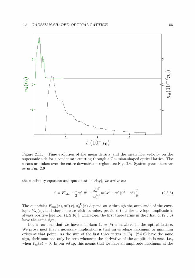
2.5. GAUSSIAN-SHAPED OPTICAL LATTICE 55
1 2 3
−5
0
5
t (104 t0)
v d(c
0)
1 2 3
1
2
3
nd(1
0−
2n
0)
Figure 2.11: Time evolution of the mean density and the mean flow velocity on thesupersonic side for a condensate emitting through a Gaussian-shaped optical lattice. Themeans are taken over the entire downstream region, see Fig. 2.6. System parameters areas in Fig. 2.9
the continuity equation and quasi-stationarity), we arrive at:
0 = E′min +
1
2m∗′
v2 +α(1)′
0
α(1)0
m∗s2 +m∗(v2 − s2)v′
v. (2.5.6)
The quantities Emin(x),m∗(x), α(1)
0 (x) depend on x through the amplitude of the enve-lope, V∞(x), and they increase with its value, provided that the envelope amplitude isalways positive [see Eq. (E.2.16)]. Therefore, the first three terms in the r.h.s. of (2.5.6)have the same sign.
Let us assume that we have a horizon (s = v) somewhere in the optical lattice.We prove next that a necessary implication is that an envelope maximum or minimumexists at that point. As the sum of the first three terms in Eq. (2.5.6) have the samesign, their sum can only be zero whenever the derivative of the amplitude is zero, i.e.,when V ′
∞(x) = 0. In our setup, this means that we have an amplitude maximum at the

56CHAPTER 2. BIRTH OF A BLACK HOLE IN A BOSE-EINSTEIN CONDENSATE
horizon. A proof of a similar result in the case of a single potential barrier, based in ahydrodynamical approximation, was already given in Ref. [56].
Now we consider the inverse implication. Assume we have V ′∞(x) = 0 (which in our
setup is the case at x = L). This implies that the first three terms in (2.5.6) are zero. Asa consequence, we are left with two possibilities:
s(L) = v(L) (2.5.7)
(i.e. a horizon) or v′ = 0. By the continuity equation, the second option implies a densityminimum, which must be ruled out in our current single Gaussian barrier setup. However,it can be a perfectly feasible result in other experimental contexts (see for instance thediscussion at the end of this section).
Finally, we note that Eq. (2.5.6) can also be written as
0 = E′min +
1
2m∗′
(v2 + 2s2) +m∗(vv′ + 2ss′) , (2.5.8)
and, as a corollary of the foregoing analysis, we find that, at the horizon, s′(L) =−v′(L)/2.
We can further exploit the previous results. For example, we can obtain the value ofthe density and the current at x = L as a function of µ:
gn(L) =2
3
µ− Emin
α(1)0
,
j(L) = nr(L)v(L) =
(
2
3
)32 (µ− Emin)
32
gα(1)0
√m∗
, (2.5.9)
which are very good approximations to the actual numerical values. Using (2.5.9) we canarrive at a differential equation for the time evolution of µ. First we note that, from thecontinuity equation, we can write:
dNL
dt= −j(L) , (2.5.10)
where NL is the number of particles contained between x = 0 and x = L. As the subsonicregion is in the Thomas-Fermi regime (see Appendix D), we can take µ ≃ gNsb/Lsb,where Nsb is the number of particles in the subsonic region and Lsb its size. As thedensity in the optical lattice is small, we can assume NL ≃ Nsb (which implies µ ∝ NL)and rewrite Eq. (2.5.10) as:
dµ
dt≃ −C (µ− Emin)
32 , (2.5.11)
where C is a positive constant independent of µ. The solution of this equation is
µ(t) = Emin +4
C2(t− t1)2, (2.5.12)
(with t1 an integration constant), which fits the numerical data of Fig. (2.9) reasonablywell. As C decreases roughly with the size of the subsonic region, we see that the largercondensate, the slower it decays, as one logically expects.
2.6. PRELIMINARY RESULTS FOR HAWKING SPECTRUM 57
Finally, we estimate the value of the Hawking temperature [see Eq. (A.1.5)] as
kBTH =~
2π
d
dx[v(x) − s(x)]x=L (2.5.13)
where we have replaced the local flow and sound velocities by their optical lattice equiv-alents. If we note that we operate in the nearly-free atom approximation (v ≪ 1) and inthe weak interaction regime (gnr ≪ ER), and derive twice the third equation (2.5.5), weobtain
kBTH ≃ ~
2πw
√
3V∞m∗ (1 − v) , (2.5.14)
which gives a good estimate of the numerical value of the Hawking temperature. Notingthat V∞ ∼ µ0,m
∗ ∼ m, we obtain kBTH ∼ ξ0µ0/w ∼ 10−2µ0 ≪ µ0. The temperatureof the condensate is typically of the order of µ0/kB, so we conclude TH ∼ 10−2T ≪T . Similar estimations for the Hawking temperature for single barrier potentials wereobtained in a hydrodynamical approximation in Refs. [56, 35].
To observe the birth of the black hole and to check that the horizon position nat-urally evolves towards the maximum of the optical lattice envelope, we have created amovie (Video 3) that shows the time evolution of the coarse-grained velocities (c, v) of theemitting condensate using the setup parameters of Fig. 2.9. At long times the predictedcoincidence between the sonic horizon and the maximum of the Gaussian envelope in thestationary regime can be clearly observed.
When applied to an ideal optical lattice, the above arguments on the position of thehorizon yield no preferred point for the location of the horizon because the envelope isuniform. Actually, in the bulk of the lattice, since V ′
∞ = 0 everywhere, the naturaloutcome [from the discussion leading to Eq. (2.5.7)] is v′ = 0 everywhere, i.e., themean velocity and (by quasi-stationarity) the mean density are also uniform, as can beobserved in Fig. 2.4. This fact only leaves two options: either the lattice bulk is subsonicor it is supersonic. The latter choice is energetically unstable (see Ref. [50]) and, as aconsequence, the subsonic regime is energetically favored in the bulk of the lattice. In therightmost region, where the potential is not present, the flow has to be supersonic, so theonly possibility for the horizon is to lie at the right extreme of the lattice, as can be seenin Fig. 2.4.
2.6 Preliminary results for Hawking spectrum
We present here a tentative study of the Hawking spectrum in the quasi-stationary black-hole regime previously described. For that purpose, we compute the S matrix treating thequasi-stationary condensate as a true stationary condensate. From Eqs. (2.2.1) (2.4.1),we see that:
Ψ(x, t) = Ψ(x, ti)e−i
∫
tti
dt′ µ(x,t′)~ (2.6.1)
for a any given t = ti. In particular, if ti is chosen such the system is already in thequasi-stationary regime, taking a given snapshot of the condensate at t = ti as an actualstationary wave function with chemical potential µ provides a good approximation since
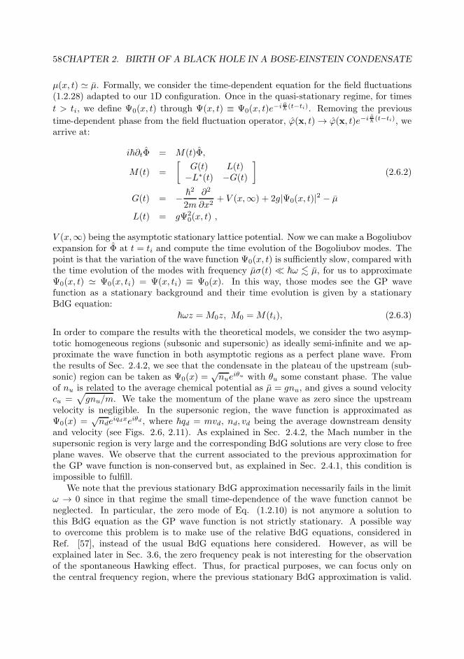
58CHAPTER 2. BIRTH OF A BLACK HOLE IN A BOSE-EINSTEIN CONDENSATE
µ(x, t) ≃ µ. Formally, we consider the time-dependent equation for the field fluctuations(1.2.28) adapted to our 1D configuration. Once in the quasi-stationary regime, for times
t > ti, we define Ψ0(x, t) through Ψ(x, t) ≡ Ψ0(x, t)e−i µ
~(t−ti). Removing the previous
time-dependent phase from the field fluctuation operator, ϕ(x, t) → ϕ(x, t)e−i µ~(t−ti), we
arrive at:
i~∂tΦ = M(t)Φ,
M(t) =
[
G(t) L(t)−L∗(t) −G(t)
]
(2.6.2)
G(t) = − ~2
2m
∂2
∂x2+ V (x,∞) + 2g|Ψ0(x, t)|2 − µ
L(t) = gΨ20(x, t) ,
V (x,∞) being the asymptotic stationary lattice potential. Now we can make a Bogoliubovexpansion for Φ at t = ti and compute the time evolution of the Bogoliubov modes. Thepoint is that the variation of the wave function Ψ0(x, t) is sufficiently slow, compared withthe time evolution of the modes with frequency µσ(t) ≪ ~ω . µ, for us to approximateΨ0(x, t) ≃ Ψ0(x, ti) = Ψ(x, ti) ≡ Ψ0(x). In this way, those modes see the GP wavefunction as a stationary background and their time evolution is given by a stationaryBdG equation:
~ωz =M0z, M0 =M(ti), (2.6.3)
In order to compare the results with the theoretical models, we consider the two asymp-totic homogeneous regions (subsonic and supersonic) as ideally semi-infinite and we ap-proximate the wave function in both asymptotic regions as a perfect plane wave. Fromthe results of Sec. 2.4.2, we see that the condensate in the plateau of the upstream (sub-sonic) region can be taken as Ψ0(x) =
√nue
iθu with θu some constant phase. The valueof nu is related to the average chemical potential as µ = gnu, and gives a sound velocitycu =
√
gnu/m. We take the momentum of the plane wave as zero since the upstreamvelocity is negligible. In the supersonic region, the wave function is approximated asΨ0(x) =
√nde
iqdxeiθd , where ~qd = mvd, nd, vd being the average downstream densityand velocity (see Figs. 2.6, 2.11). As explained in Sec. 2.4.2, the Mach number in thesupersonic region is very large and the corresponding BdG solutions are very close to freeplane waves. We observe that the current associated to the previous approximation forthe GP wave function is non-conserved but, as explained in Sec. 2.4.1, this condition isimpossible to fulfill.
We note that the previous stationary BdG approximation necessarily fails in the limitω → 0 since in that regime the small time-dependence of the wave function cannot beneglected. In particular, the zero mode of Eq. (1.2.10) is not anymore a solution tothis BdG equation as the GP wave function is not strictly stationary. A possible wayto overcome this problem is to make use of the relative BdG equations, considered inRef. [57], instead of the usual BdG equations here considered. However, as will beexplained later in Sec. 3.6, the zero frequency peak is not interesting for the observationof the spontaneous Hawking effect. Thus, for practical purposes, we can focus only onthe central frequency region, where the previous stationary BdG approximation is valid.
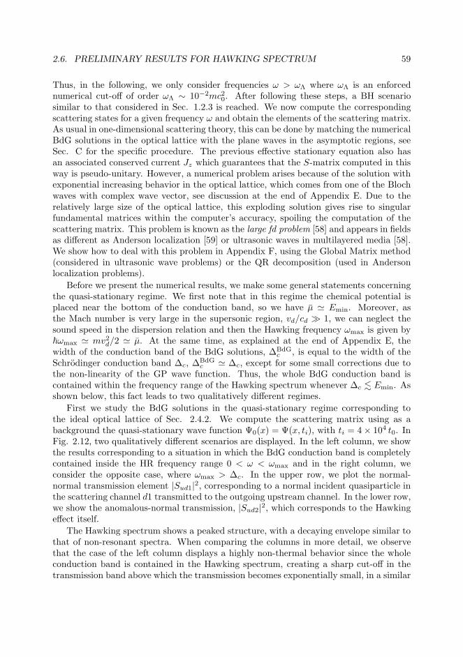
2.6. PRELIMINARY RESULTS FOR HAWKING SPECTRUM 59
Thus, in the following, we only consider frequencies ω > ωΛ where ωΛ is an enforcednumerical cut-off of order ωΛ ∼ 10−2mc20. After following these steps, a BH scenariosimilar to that considered in Sec. 1.2.3 is reached. We now compute the correspondingscattering states for a given frequency ω and obtain the elements of the scattering matrix.As usual in one-dimensional scattering theory, this can be done by matching the numericalBdG solutions in the optical lattice with the plane waves in the asymptotic regions, seeSec. C for the specific procedure. The previous effective stationary equation also hasan associated conserved current Jz which guarantees that the S-matrix computed in thisway is pseudo-unitary. However, a numerical problem arises because of the solution withexponential increasing behavior in the optical lattice, which comes from one of the Blochwaves with complex wave vector, see discussion at the end of Appendix E. Due to therelatively large size of the optical lattice, this exploding solution gives rise to singularfundamental matrices within the computer’s accuracy, spoiling the computation of thescattering matrix. This problem is known as the large fd problem [58] and appears in fieldsas different as Anderson localization [59] or ultrasonic waves in multilayered media [58].We show how to deal with this problem in Appendix F, using the Global Matrix method(considered in ultrasonic wave problems) or the QR decomposition (used in Andersonlocalization problems).
Before we present the numerical results, we make some general statements concerningthe quasi-stationary regime. We first note that in this regime the chemical potential isplaced near the bottom of the conduction band, so we have µ ≃ Emin. Moreover, asthe Mach number is very large in the supersonic region, vd/cd ≫ 1, we can neglect thesound speed in the dispersion relation and then the Hawking frequency ωmax is given by~ωmax ≃ mv2d/2 ≃ µ. At the same time, as explained at the end of Appendix E, thewidth of the conduction band of the BdG solutions, ∆BdG
c , is equal to the width of theSchrodinger conduction band ∆c, ∆
BdGc ≃ ∆c, except for some small corrections due to
the non-linearity of the GP wave function. Thus, the whole BdG conduction band iscontained within the frequency range of the Hawking spectrum whenever ∆c . Emin. Asshown below, this fact leads to two qualitatively different regimes.
First we study the BdG solutions in the quasi-stationary regime corresponding tothe ideal optical lattice of Sec. 2.4.2. We compute the scattering matrix using as abackground the quasi-stationary wave function Ψ0(x) = Ψ(x, ti), with ti = 4× 10⁴ t0. InFig. 2.12, two qualitatively different scenarios are displayed. In the left column, we showthe results corresponding to a situation in which the BdG conduction band is completelycontained inside the HR frequency range 0 < ω < ωmax and in the right column, weconsider the opposite case, where ωmax > ∆c. In the upper row, we plot the normal-normal transmission element |Sud1|2, corresponding to a normal incident quasiparticle inthe scattering channel d1 transmitted to the outgoing upstream channel. In the lower row,we show the anomalous-normal transmission, |Sud2|2, which corresponds to the Hawkingeffect itself.
The Hawking spectrum shows a peaked structure, with a decaying envelope similar tothat of non-resonant spectra. When comparing the columns in more detail, we observethat the case of the left column displays a highly non-thermal behavior since the wholeconduction band is contained in the Hawking spectrum, creating a sharp cut-off in thetransmission band above which the transmission becomes exponentially small, in a similar

60CHAPTER 2. BIRTH OF A BLACK HOLE IN A BOSE-EINSTEIN CONDENSATE
0.1 0.2 0.3 0.4 0.5 0.6 0.7 0.8 0.9
0.01
0.02
0.03
0.04
0.05
0.06
0.07
0.08
ω (mc2
0)
|Su
d2|2
0.4 0.6 0.8
0.2
0.4
0.6
0.8
ω (mc2
0)
104×
|Su
d2|2
0.1 0.2 0.3 0.4 0.5 0.6 0.7 0.8
0.05
0.1
0.15
0.2
0.25
0.3
ω (mc2
0)
|Su
d2|2
0.3 0.4 0.5 0.6 0.7 0.8
0.2
0.4
0.6
0.8
ω (mc2
0)
104×
|Su
d2|2
0.1 0.2 0.3 0.4 0.5 0.6 0.7 0.8 0.9
0.1
0.2
0.3
0.4
0.5
0.6
0.7
0.8
0.9
ω (mc2
0)
|Su
d1|2
0.1 0.2 0.3 0.4 0.5 0.6 0.7 0.8
0.1
0.2
0.3
0.4
0.5
0.6
0.7
0.8
0.9
ω (mc2
0)
|Su
d1|2
Figure 2.12: Hawking spectrum for two different simulations for an ideal optical lattice.The BdG solutions are computed on top of the quasi-stationary mean-field backgroundprovided by the wave function evaluated at a time 4× 10⁴ t0. Both graphs are computedwith τ = 500 t0, L = 400µm, nosc = 30, N = 104, and ωtr = 2π × 4 kHz, and thevarying parameters are the long-time potential amplitude V∞ and the lattice spacingd. We have ξ0 = 0.3175µm. Left panel: V∞ = 2.13 mc20 and d = 2.36ξ0, which givesEmin = 0.91 mc20 and ∆c = 0.47 mc20. The long time parameters of the quasi-stationaryflow are µ ≃ ωmax = 0.96 mc20, cu = 0.98 c0, vd = 1.39 c0 and cd = 0.02 c0. Right panel:V∞ = 1.86 mc20 and d = 1.91ξ0, which gives Emin = 0.85 mc20 and ∆c = 0.95 mc20. Thelong time parameters of the quasi-stationary flow are µ ≃ ωmax = 0.90 mc20, cu = 0.95 c0,vd = 1.34 c0 and cd = 0.03 c0.
way to the Schrodinger transmission of Fig. 2.7.
By comparing both rows, we clearly see that the transmission band corresponds almostentirely to normal-normal transmission while the anomalous-normal transmission playsa secondary role. We can understand this effect by inspecting the form of the BdGsolutions in the optical lattice and in the supersonic region. Due to the low value of the
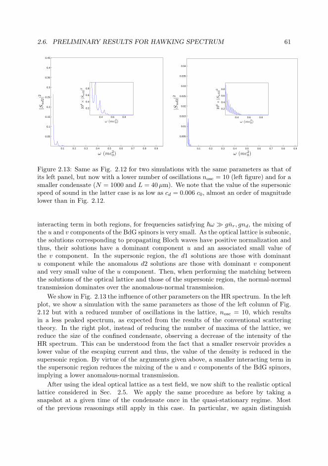
2.6. PRELIMINARY RESULTS FOR HAWKING SPECTRUM 61
0.1 0.2 0.3 0.4 0.5 0.6 0.7 0.8 0.9
0.05
0.1
0.15
0.2
0.25
0.3
0.35
0.4
0.45
ω (mc2
0)
|Su
d2|2
0.4 0.6 0.8
0.2
0.4
0.6
0.8
ω (mc2
0)
104×
|Su
d2|2
0.1 0.2 0.3 0.4 0.5 0.6 0.7 0.8 0.9
0.005
0.01
0.015
0.02
0.025
0.03
0.035
0.04
ω (mc2
0)
|Su
d2|2
0.4 0.6 0.8
0.2
0.4
0.6
0.8
ω (mc2
0)
106×
|Su
d2|2
Figure 2.13: Same as Fig. 2.12 for two simulations with the same parameters as that ofits left panel, but now with a lower number of oscillations nosc = 10 (left figure) and for asmaller condensate (N = 1000 and L = 40µm). We note that the value of the supersonicspeed of sound in the latter case is as low as cd = 0.006 c0, almost an order of magnitudelower than in Fig. 2.12.
interacting term in both regions, for frequencies satisfying ~ω ≫ gnr, gnd, the mixing ofthe u and v components of the BdG spinors is very small. As the optical lattice is subsonic,the solutions corresponding to propagating Bloch waves have positive normalization andthus, their solutions have a dominant component u and an associated small value ofthe v component. In the supersonic region, the d1 solutions are those with dominantu component while the anomalous d2 solutions are those with dominant v componentand very small value of the u component. Then, when performing the matching betweenthe solutions of the optical lattice and those of the supersonic region, the normal-normaltransmission dominates over the anomalous-normal transmission.
We show in Fig. 2.13 the influence of other parameters on the HR spectrum. In the leftplot, we show a simulation with the same parameters as those of the left column of Fig.2.12 but with a reduced number of oscillations in the lattice, nosc = 10, which resultsin a less peaked spectrum, as expected from the results of the conventional scatteringtheory. In the right plot, instead of reducing the number of maxima of the lattice, wereduce the size of the confined condensate, observing a decrease of the intensity of theHR spectrum. This can be understood from the fact that a smaller reservoir provides alower value of the escaping current and thus, the value of the density is reduced in thesupersonic region. By virtue of the arguments given above, a smaller interacting term inthe supersonic region reduces the mixing of the u and v components of the BdG spinors,implying a lower anomalous-normal transmission.
After using the ideal optical lattice as a test field, we now shift to the realistic opticallattice considered in Sec. 2.5. We apply the same procedure as before by taking asnapshot at a given time of the condensate once in the quasi-stationary regime. Mostof the previous reasonings still apply in this case. In particular, we again distinguish
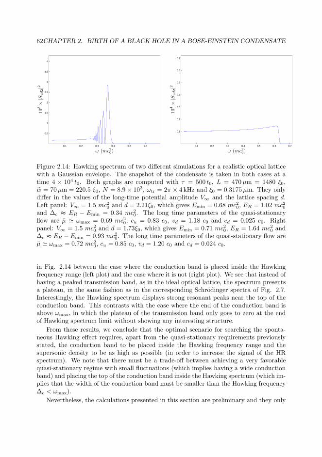
62CHAPTER 2. BIRTH OF A BLACK HOLE IN A BOSE-EINSTEIN CONDENSATE
0.1 0.2 0.3 0.4 0.5 0.6
0.5
1
1.5
2
2.5
3
3.5
4
ω (mc2
0)
103×
|Su
d2|2
0.1 0.2 0.3 0.4 0.5 0.6 0.7
0.1
0.2
0.3
0.4
0.5
0.6
0.7
ω (mc2
0)
104×
|Su
d2|2
Figure 2.14: Hawking spectrum of two different simulations for a realistic optical latticewith a Gaussian envelope. The snapshot of the condensate is taken in both cases at atime 4 × 10⁴ t0. Both graphs are computed with τ = 500 t0, L = 470µm = 1480 ξ0,w = 70µm = 220.5 ξ0, N = 8.9 × 10³, ωtr = 2π × 4 kHz and ξ0 = 0.3175µm. They onlydiffer in the values of the long-time potential amplitude V∞ and the lattice spacing d.Left panel: V∞ = 1.5 mc20 and d = 2.21ξ0, which gives Emin = 0.68 mc20, ER = 1.02 mc20and ∆c ≈ ER − Emin = 0.34 mc20. The long time parameters of the quasi-stationaryflow are µ ≃ ωmax = 0.69 mc20, cu = 0.83 c0, vd = 1.18 c0 and cd = 0.025 c0. Rightpanel: V∞ = 1.5 mc20 and d = 1.73ξ0, which gives Emin = 0.71 mc20, ER = 1.64 mc20 and∆c ≈ ER − Emin = 0.93 mc20. The long time parameters of the quasi-stationary flow areµ ≃ ωmax = 0.72 mc20, cu = 0.85 c0, vd = 1.20 c0 and cd = 0.024 c0.
in Fig. 2.14 between the case where the conduction band is placed inside the Hawkingfrequency range (left plot) and the case where it is not (right plot). We see that instead ofhaving a peaked transmission band, as in the ideal optical lattice, the spectrum presentsa plateau, in the same fashion as in the corresponding Schrodinger spectra of Fig. 2.7.Interestingly, the Hawking spectrum displays strong resonant peaks near the top of theconduction band. This contrasts with the case where the end of the conduction band isabove ωmax, in which the plateau of the transmission band only goes to zero at the endof Hawking spectrum limit without showing any interesting structure.
From these results, we conclude that the optimal scenario for searching the sponta-neous Hawking effect requires, apart from the quasi-stationary requirements previouslystated, the conduction band to be placed inside the Hawking frequency range and thesupersonic density to be as high as possible (in order to increase the signal of the HRspectrum). We note that there must be a trade-off between achieving a very favorablequasi-stationary regime with small fluctuations (which implies having a wide conductionband) and placing the top of the conduction band inside the Hawking spectrum (which im-plies that the width of the conduction band must be smaller than the Hawking frequency∆c < ωmax).
Nevertheless, the calculations presented in this section are preliminary and they only

2.7. CONCLUSIONS AND OUTLOOK 63
give us an approximated idea of the situation in the quasi-stationary regime. Severalpoints should be addressed in a more complete calculation. First, one has to take intoaccount the large but finite size of the confined subsonic region, which would introducea hard-wall boundary condition in the BdG equations at x = 0. Second, a more rigor-ous model should be introduced for computing the quasi-stationary modes that includesalso the lower frequency modes. This could be made, as noted before, by employing therelative BdG equations [57] instead of the usual BdG equations. Finally, in order to com-pute the corresponding expectation values, one should also take into account the initialquantum state of the system at t = 0, which is expected to be a thermal mixture of theinitial quasiparticle confined modes (see Sec. D.2 for more details), and compute its timeevolution, which in the Bogoliubov approximation would correspond to a full integrationof the time-dependent BdG equations. All these tasks represent harder calculations fromboth a theoretical and a computational point of view that are left for future works.
2.7 Conclusions and outlook
Within a mean-field description, we have investigated the process whereby an initiallyconfined atom condensate is coherently outcoupled as the barrier on one side is graduallylowered. The goal has been to identify the barrier-lowering protocol which best leads to aquasi-stationary sonic black hole located at the interface between subsonic and supersonicflow. We find that the use of an optical lattice for the lowered barrier helps to achieve aregime of quasi-stationary flow with a minimal value of the fluctuation spread. First wehave focused on an optical lattice of finite length and uniform amplitude. We also findthat the long-time band structure of the optical lattice greatly influences the asymptoticbehavior of the emitted atom flow. Within this class of setups, the best quasi-stationaryflow is achieved when the lowest conduction band is broad and the initial chemical po-tential lies not much high above the bottom of the final conduction band. In the optimalcases, the relative value of the spatial fluctuations can be as small as σ(t) ∼ 10−4. Whenwe replace the uniform amplitude of the optical lattice by a more realistic Gaussian enve-lope, we find that the results are similar to those of a uniform lattice with the amplitudeof the envelope maximum. Quite interestingly, we argue analytically and check numeri-cally that, in the quasi-stationary regime, the horizon separating the regions of subsonicand supersonic flow is pinned down right at the Gaussian maximum. We also find thatthe Gaussian envelope is quite efficient in guaranteeing a small deviation from the idealstationary flow.
The results here obtained are also of relevance in the context of quantum transport.Atom flow through a sonic black hole may also be viewed as one of the paradigms of atomquantum transport through a barrier [28]. In particular, the setup here presented can beused to provide a quasi-stationary supersonic current, with a well defined velocity (seeFigs. 2.6, 2.11).
After the previous mean-field calculation, we have presented a preliminary study ofthe Hawking spectrum, in which we assume the condensate to be truly stationary andsemi-infinite in order to match with the usual theoretical descriptions. We find thattwo qualitative regimes can be distinguished depending on whether the top of the BdG
64CHAPTER 2. BIRTH OF A BLACK HOLE IN A BOSE-EINSTEIN CONDENSATE
conduction band lies below or above the Hawking frequency. In particular, when thetop of the conduction band is placed within the frequency range of the Hawking effect,the system displays a highly structured Hawking spectrum which provides a promisingscenario for the detection of the Hawking effect. However, we remark that these resultsare only preliminary. A more detailed future study should confirm the validity of theseobservations.
Chapter 3Quantum signatures of spontaneous
Hawking radiation
3.1 Introduction
In the previous chapter, we have numerically studied the birth of a quasi-stationary blackhole in a Bose-Einstein condensate within a realistic experimental scenario. The ques-tion now is how to detect the spontaneous Hawking radiation above the previous quasi-stationary background. The answer is highly non-trivial. On one hand, in a real setupthe system is always at a finite non-zero temperature and then, the state of the system isnot strictly the vacuum of the incoming scattering modes. In particular, the stimulatedsignal arising from the thermal occupation of phonon modes can easily overshadow thespontaneous signal due to the genuine quantum Hawking effect.
On the other hand, a clear detection of the Hawking effect should be able to distin-guish the quantum origin of the Hawking effect from the small perturbations around thecoherent condensate wave function that are impossible to avoid in a realistic scenario, asdiscussed and quantified in the previous chapter. The point is that the Bogoliubov-deGennes equations describe both phenomena: linearized collective motion and quantumquasiparticle excitation. The former is fully describable within a mean-field picture; thelatter reflects the presence of a many-body ground state (the Bogoliubov vacuum) withstrong pair correlations.
Detection schemes based on density-density correlations in real space are not able todistinguish unambiguously the spontaneous Hawking signal [15, 31]. The mere measure-ment of phonon [60] or atom [22] intensity spectra would not permit those distinctionseither.
Hawking radiation is a fundamental quantum phenomenon that results from the im-possibility of identifying the vacuum of incoming quasiparticles with that of outgoingquasiparticles [61]. Specifically, the incoming vacuum is a squeezed state of outgoingquasiparticles. In this respect, it has been long recognized in quantum optical contexts
65

66CHAPTER 3. QUANTUM SIGNATURES OF SPONTANEOUS HAWKING RADIATION
[62, 33] that correlation functions characterizing the electromagnetic radiation satisfyCauchy-Schwarz (CS) type inequalities, which can, however, be violated in the deepquantum regime, particularly by squeezed light. Thus, the violation of CS inequalitiesis generally regarded as a conclusive signature of quantum behavior. We devote part ofthis chapter to show that the violation of certain CS inequalities is indeed a signal ofthe presence of spontaneous HR and that the sole presence of linearized collective motionaround the stationary wave function or stimulated phonon signal could not provide suchviolation. As a result, we identify this particular CS violation as an unequivocal smokinggun of the presence of spontaneous HR. The same cannot be said about other CS viola-tions that are always present in a Bogoliubov vacuum; for example, those associated withthe paired atom modes k,−k in a condensate at rest. Such CS violations will appear inother correlation functions.
An alternative scheme to identify deep quantum behavior relies on the detection of en-tanglement between the various outgoing radiation channels from a sonic horizon [63, 64].A recent work has addressed the possibility of detecting entanglement through density-density correlations in Fourier space [65]. Approaches based on entanglement detectionhave been also proposed in analogous contexts such as inflationary cosmology [66], as-trophysical black holes [67], general relativistic quantum fields [68], or other black-holeanalogs [11, 69]. In the present chapter, we establish in great detail the links between thework developed in the present thesis, based on the detection of violation of CS inequal-ities, and the works of Refs. [64, 63], based on the detection of entanglement, unifyingboth approaches.
We also study in this chapter the potential measurability of the previous criteriain specific detection schemes. Importantly, by introducing envelope-modulated Fouriertransforms we explicitly take into account the role played by the spatial location of theasymptotic regions. This allows us to show that the violation of only quadratic CSinequalities can be measured. In particular, we prove that the complete implementationof the generalized Peres-Horodecki (GPH) criterion or the quartic CS violation requires theknowledge of parameters that are impossible or very difficult to measure, at least withinthe class of detection schemes here considered. However, we also show that this does notrepresent an important limitation in practice, since, under rather broad conditions, allthe previous criteria become equivalent.
Although the content developed in this chapter is motivated by the quest for the ob-servation of spontaneous HR, the results here obtained are also of relevance in neighboringfields such as quantum optics [70, 71] and quantum information physics [72, 73], as wellas in the broader topic of bosonic condensates [74, 75].
We devote Sections 3.2-3.3 to review general signatures of quantum behavior and dis-cuss the general properties of CS inequalities and entanglement. We apply these conceptsto the specific scenario of analog Hawking radiation in Sec. 3.4 and unify the previous cri-teria under certain conditions. In Section 3.5, we discuss the possibility of experimentallyverifying the discussed detection schemes. Finally, in Section 3.6, we present numericalresults on the detection of the CS violation in typical BH setups. The conclusions arepresented in Sec. 3.7. We explain in Sec. G the parametrization of the scattering matrixand of the computation of the correlation functions used in the main text.

3.2. GENERAL SIGNATURES OF QUANTUM BEHAVIOR 67
3.2 General signatures of quantum behavior
We start by reviewing some general signatures of quantum behavior. For illustrativepurposes, we discuss the criteria usually considered in quantum optics [62, 33]. We focuson the properties of the normalized second-order correlation function, which for light isdefined as
g(2)ij (τ) ≡
〈a†i (0)a†j(τ)aj(τ)ai(0)〉
〈a†i (0)ai(0)〉〈a†j(0)aj(0)〉
, (3.2.1)
where ai(t) is the Heisenberg operator for photon mode i, and the average is quantum-statistical. The correlation function for classical light is obtained by removing the quan-tum average and replacing the Heisenberg operators ai(t) by complex numbers. Thefollowing inequalities can be proven for classical light:
1 ≤ g(2)ii (0), (3.2.2)
g(2)ii (τ) ≤ g
(2)ii (0), (3.2.3)
[
g(2)ij (τ)
]2
≤ g(2)ii (0)g
(2)jj (0) , (i 6= j) . (3.2.4)
These inequalities are satisfied not only classically but also by quantum thermal states athigh temperature. They are also satisfied by chaotic and coherent states.
The violation of any of the above inequalities is a signature of deep quantum behavior.States violating (3.2.2) are said to show sub-Poissonian statistics. Violation of (3.2.3)reflects anti-bunching. Expression (3.2.4) is a CS inequality. States which violate itat τ = 0 are said to exhibit two-mode sub-Poissonian statistics. In general, the proof of(3.2.4) requires the system to be described by a positive (Glauber-Sudarshan) P function.Some quantum states such as two-mode squeezed states may not satisfy this conditionand thus can violate (3.2.4).
Another possible signature of quantum behavior is the presence of entanglement [33],which also requires the system to be described by non-classical statistics. We defineprecisely in the next section the concept of entanglement considered throughout thiswork.
3.3 General properties of Cauchy-Schwarz inequalities
and Peres-Horodecki criterion
We now study in more detail the criteria previously discussed. In particular, we focuson two specific signatures: the violation of CS inequalities and the entanglement of thesystem, which are the only interesting ones for studying HR as we will explain in Sec. 3.4.First, we review the mathematical CS inequalities for operators in a Hilbert space, whichare always fulfilled, see for instance Ref. [76]. We define the scalar product associated toa state ρ for two operator A, B as:
(A, B) ≡ 〈A†B〉 = Tr(ρA†B). (3.3.1)

68CHAPTER 3. QUANTUM SIGNATURES OF SPONTANEOUS HAWKING RADIATION
where the expectation value of an operator O is taken over the state of the system, de-scribed by the density matrix ρ, 〈O〉 = Tr(ρO). It is easy to check that the previousproduct satisfies the usual properties of a scalar product. Thus, it satisfies the mathe-matical Cauchy-Schwarz inequality:
| 〈A†B〉 |2 ≤ 〈A†A〉 〈B†B〉 (3.3.2)
In particular, the previous inequality implies for B = 1 that
| 〈A〉 |2 = | 〈A†〉 |2 ≤ 〈A†A〉 (3.3.3)
For our purposes, we consider, in a general context, correlations between two givenquantum modes i, j, whose corresponding annihilation operators are γi,j . The first-ordercorrelation functions are given by
gij ≡ 〈γ†i γj〉 , cij ≡ 〈γiγj〉 , (3.3.4)
The mathematical CS inequality associated to the previous correlation functions are ob-tained by substituting A = γi and B = γj in Eq. (3.3.2)
|gij |2 = | 〈γ†i γj〉 |2 ≤ 〈γ†i γi〉 〈γ†j γj〉 = giigjj (3.3.5)
Thus, the CS inequality |gij |2 ≤ giigjj is always satisfied and can never be violated. On
the other hand, taking A = γ†i and B = γj , we arrive at:
|cij |2 = | 〈γiγj〉 |2 ≤ 〈γiγ†i 〉 〈γ†j γj〉 = (gii + 1)gjj . (3.3.6)
Interestingly, the mathematical CS inequality for quantum operators is |cij |2 ≤ (gii+1)gjj ,instead of the classical CS inequality |cij |2 ≤ giigjj , always satisfied in a classical context,in a similar fashion to Eq. (3.2.4). This leaves the possibility of violating the classical CSinequality, which we can quantify by introducing the following magnitude:
∆ij ≡ |cij |2 − giigjj > 0 . (3.3.7)
The fulfillment of the previous condition reflects the quantum nature of the state of thesystem. We can also quantify the relative degree of CS violation by introducing
δij ≡|cij |2giigjj
> 1 . (3.3.8)
We will refer indistinctly to Eqs. (3.3.7), (3.3.8) as the quadratic CS violation.We can extend the previous idea to the following second-order correlation function:
Γij ≡ 〈γ†i γ†j γj γi〉 > 0 , (3.3.9)
A similar reasoning leads to the mathematical CS inequality:
|Γij |2 = | 〈γ†i γiγ†j γj〉 |2 ≤ 〈γ†i γiγ
†i γi〉 〈γ
†j γj γ
†j γj〉
= (Γii + gii)(Γjj + gjj) (3.3.10)

3.3. GENERAL PROPERTIES OF QUANTUM SIGNATURES 69
which also leaves the possibility of violating the classical CS inequality |Γij |2 ≤ ΓiiΓjj ,as quantified by
Θij ≡ Γij −√
ΓiiΓjj > 0 . (3.3.11)
We can also measure the relative degree of violation using
θij ≡Γij
√
ΓiiΓjj
> 1 . (3.3.12)
In analogy to the quadratic CS violation, we will refer to the previous conditions as quarticCS violation. Both quadratic and quartic violations are signatures of quantum behaviorsince they cannot be satisfied in a classical context.
Another possible signature of the quantum character of the system is the presence ofentanglement between the modes i, j. In this work, we follow the convention of definingentanglement as the non-separability of the state of the system. We say that a two-modestate ρ is separable when it can be decomposed as:
ρ =∑
n
pnρ(i)n ⊗ ρ(j)n (3.3.13)
where ρ(i,j)n are states of the Hilbert subspace associated to the i, j modes, respectively. In
order to characterize the entanglement, we make use of the generalized Peres-Horodecki(GPH) criterion [77, 78]. The GPH criterion is based on the fact that, if ρ is separable,by taking the partial transpose of ρ with respect to only the Hilbert space associated tothe mode j, we obtain an operator ρt that is also a physical density matrix, satisfying theusual properties of quantum states.
For studying the partial transpose of ρ, ρt, we first define the vector X ≡ [qi, pi, qj , pj ]T
and the corresponding phase space variables X ≡ [qi, pi, qj , pj ]T , where the phase space
operators qk, pk are related to the annihilation operator of the modes k = i, j throughγk = (qk + ipk)/
√2. The commutation relations between the components of X are
[Xα, Xβ] = iLαβ, where Lαβ is a 4× 4 matrix of the form
L =
[
J 00 J
]
, J =
[
0 1−1 0
]
(3.3.14)
with J the symplectic matrix in two dimensions. In order to characterize ρt, we studythe effect of partial transposition on the Wigner function. The Wigner function of thestate ρ is given by:
W (X) ≡ 1
(2π)2
∫
d2q′ 〈q − q′
2|ρ|q + q′
2〉 eiq′p (3.3.15)
with q = (qi, qj), p = (pi, pj). By transposing the matrix elements of ρ with respect tothe Hilbert space of the mode j, it is straightforward to show from the previous definitionthat the Wigner distribution associated to ρt is Wt(qi, pi, qj , pj) = W (qi, pi, qj ,−pj), or,in a more compact form
Wt(X) =W (ΛX), Λ = diag[1, 1, 1,−1]. (3.3.16)
70CHAPTER 3. QUANTUM SIGNATURES OF SPONTANEOUS HAWKING RADIATION
We note, from this result, that partial transposition amounts to a local time inversion onthe second variable [78]. The partial transpose has important effects when consideringthe uncertainties of the phase space operators. If we define the operator
Y =
4∑
α=1
uα∆Xα, (3.3.17)
where ∆X ≡ X − 〈X〉, we have that 〈Y †Y 〉 ≥ 0, with uα the components of an arbitraryfour dimensional complex vector. The previous relation can be written compactly invectorial notation as:
u†Mu ≥ 0 (3.3.18)
M ≡ V + iL
2
V being the covariance matrix with matrix elements Vαβ = 12 〈∆Xα,∆Xβ〉 and ∆Xα,∆Xβ
the anticommutator. We see that Eq. (3.3.18) represents an alternative expression of theuncertainty principle. In particular, as it holds for any complex vector u, the uncertaintyprinciple simply states that M must be a non-negative matrix, M ≥ 0. Since L is aconstant matrix independent of the state ρ, we only have to compute the covariance ma-trix V for obtaining the matrix M . As well-known from quantum optics, the symmetriccovariances can be computed using the Wigner function [79]:
〈Xα〉 =
∫
d4X XαW (X) (3.3.19)
〈∆Xα,∆Xβ〉 =
∫
d4X ∆Xα∆XβW (X)
When considering ρt, the state obtained by the partial transposition of ρ, and followingan analog reasoning, we find that the uncertainty principle for ρt is simply given by thecondition Mt ≥ 0, where:
Mt ≡ Vt + iL
2(3.3.20)
Now, Vt is the same covariance matrix as V but with the expectation values evaluated inthe state ρt. Taking into account Eqs. 3.3.16,3.3.19, we see that Vt = ΛV Λ.
The GPH criterion is based in the fact that ifMt is a non positive-semidefinite matrix,the state is entangled, since if the state ρ is separable, ρt must be a physical state andthen, the associated uncertainty principle reads Mt ≥ 0. Since M is non-negative as ρ isa physical density matrix, Mt is non-negative if and only if detMt ≥ 0. The conditionsdetM,Mt ≥ 0 are respectively equivalent to P±
ij ≥ 0, where:
P±ij ≡ detAi detAj +
(
1
4∓ detCij
)2
(3.3.21)
− tr(JAiJCijJAjJCTij)−
1
4(detAi + detAj),
3.3. GENERAL PROPERTIES OF QUANTUM SIGNATURES 71
The matrices Ai, Aj , Cij are 2× 2 submatrices of the covariance matrix V :
V =
[
Ai Cij
CTij Aj
]
(3.3.22)
We note that P+ij ≥ 0 is always satisfied provided that ρ is a physical density matrix.
However, when P−ij < 0, the state ρt is not a physical state which implies that the state
ρ is not separable. We can put together both conditions by defining the GPH functionPij as:
Pij ≡ detAi detAj +
(
1
4− | detCij |
)2
(3.3.23)
− tr(JAiJCijJAjJCTij)−
1
4(detAi + detAj),
Thus, if Pij < 0, the state is automatically entangled. This is the final form of the GPHcriterion that we will use in this work. We note that, whenever detCij ≥ 0, the state isseparable, as Pij = P+
ij ≥ 0, so only states with detCij < 0 can be entangled.We can compute explicitly the GPH function in terms of the first order correlation
functions of Eq. (3.3.4). Hereafter, we focus for simplicity on the usual case wherethe annihilation and destruction operators have zero mean value [if not, we can simplymodify the definition of the correlations in Eq. (3.3.4) by substituting the γ operators bytheir fluctuations]. The matrices Ai,j and Cij can be written in terms of the first-ordercorrelation functions as:
Ak =
(
gkk +1
2
)
I2 +
[
Re ckk Im ckkIm ckk −Re ckk
]
(3.3.24)
Cij =
[
Re(gij − cij) Im(gij + cij)Im(−gij + cij) Re(gij − cij)
]
, (3.3.25)
with the index k = i, j and I2 the 2×2 identity matrix. Then, using Eqs. (3.3.23),(3.3.24),we obtain:
Pij = [giigjj − |cij |2][(gii + 1)(gjj + 1)− |cij |2] + 4
(
gii +1
2
)
Re(gijc∗jjcij) (3.3.26)
+ 4
(
gjj +1
2
)
Re(gijciic∗ij)− 2Re(c2ijc
∗iic
∗jj)− 2Re(g2ijciic
∗jj) + |cii|2|cjj |2 + |gij |4
− |gij |2(gii + gjj + 2giigjj + 2|cij |2)− gii(gii + 1)|cjj |2 − gjj(gjj + 1)|cii|2 .This expression applies whenever |cij | ≥ |gij |. For |cij | < |gij |, we have detCij > 0 and
the state is separable so there is no need of using the GPH function. We finally remarkthat, in the particular case of Gaussian states, the GPH criterion is also a necessarycondition for entanglement [78]. Thus, for Gaussian states, the GPH criterion is equivalentto the entanglement of the system. We can understand this relation from the fact thatGaussian states are completely determined by their second momentums and, precisely,the GPH criterion characterizes entanglement only involving the second momentums ofthe distribution
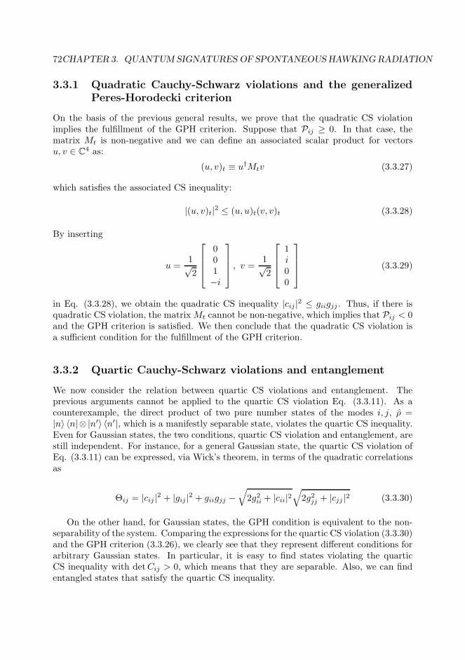
72CHAPTER 3. QUANTUM SIGNATURES OF SPONTANEOUS HAWKING RADIATION
3.3.1 Quadratic Cauchy-Schwarz violations and the generalized
Peres-Horodecki criterion
On the basis of the previous general results, we prove that the quadratic CS violationimplies the fulfillment of the GPH criterion. Suppose that Pij ≥ 0. In that case, thematrix Mt is non-negative and we can define an associated scalar product for vectorsu, v ∈ C4 as:
(u, v)t ≡ u†Mtv (3.3.27)
which satisfies the associated CS inequality:
|(u, v)t|2 ≤ (u, u)t(v, v)t (3.3.28)
By inserting
u =1√2
001−i
, v =1√2
1i00
(3.3.29)
in Eq. (3.3.28), we obtain the quadratic CS inequality |cij |2 ≤ giigjj . Thus, if there isquadratic CS violation, the matrixMt cannot be non-negative, which implies that Pij < 0and the GPH criterion is satisfied. We then conclude that the quadratic CS violation isa sufficient condition for the fulfillment of the GPH criterion.
3.3.2 Quartic Cauchy-Schwarz violations and entanglement
We now consider the relation between quartic CS violations and entanglement. Theprevious arguments cannot be applied to the quartic CS violation Eq. (3.3.11). As acounterexample, the direct product of two pure number states of the modes i, j, ρ =|n〉 〈n|⊗ |n′〉 〈n′|, which is a manifestly separable state, violates the quartic CS inequality.Even for Gaussian states, the two conditions, quartic CS violation and entanglement, arestill independent. For instance, for a general Gaussian state, the quartic CS violation ofEq. (3.3.11) can be expressed, via Wick’s theorem, in terms of the quadratic correlationsas
Θij = |cij |2 + |gij |2 + giigjj −√
2g2ii + |cii|2√
2g2jj + |cjj |2 (3.3.30)
On the other hand, for Gaussian states, the GPH condition is equivalent to the non-separability of the system. Comparing the expressions for the quartic CS violation (3.3.30)and the GPH criterion (3.3.26), we clearly see that they represent different conditions forarbitrary Gaussian states. In particular, it is easy to find states violating the quarticCS inequality with detCij > 0, which means that they are separable. Also, we can findentangled states that satisfy the quartic CS inequality.
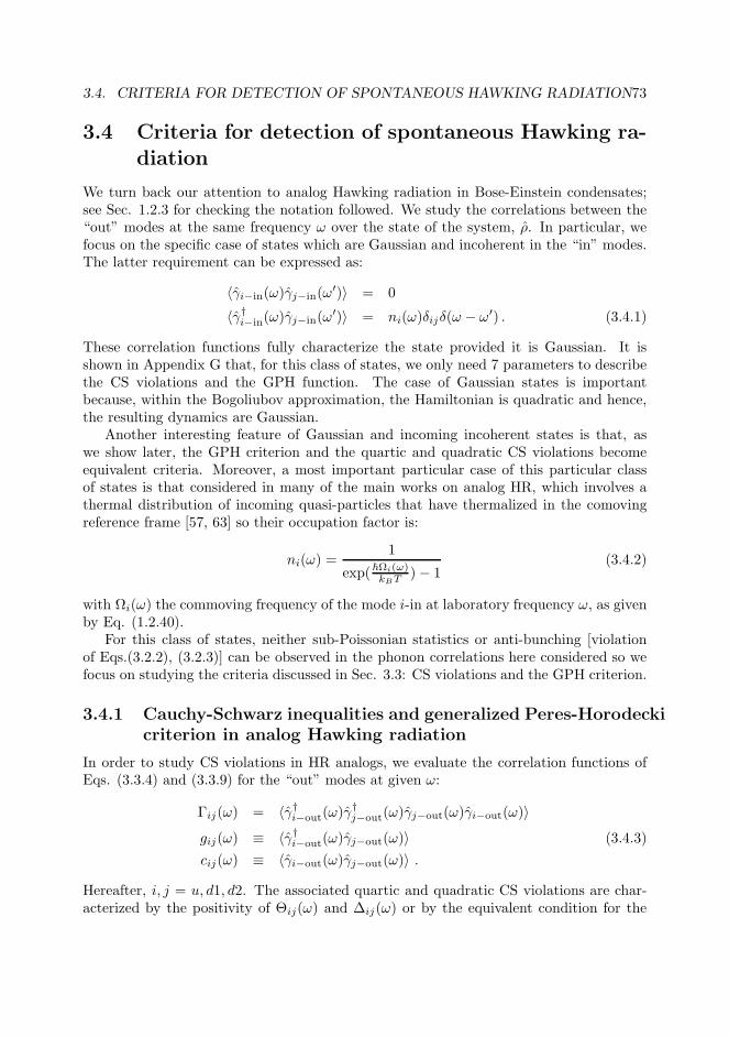
3.4. CRITERIA FOR DETECTION OF SPONTANEOUS HAWKING RADIATION73
3.4 Criteria for detection of spontaneous Hawking ra-
diation
We turn back our attention to analog Hawking radiation in Bose-Einstein condensates;see Sec. 1.2.3 for checking the notation followed. We study the correlations between the“out” modes at the same frequency ω over the state of the system, ρ. In particular, wefocus on the specific case of states which are Gaussian and incoherent in the “in” modes.The latter requirement can be expressed as:
〈γi−in(ω)γj−in(ω′)〉 = 0
〈γ†i−in(ω)γj−in(ω′)〉 = ni(ω)δijδ(ω − ω′) . (3.4.1)
These correlation functions fully characterize the state provided it is Gaussian. It isshown in Appendix G that, for this class of states, we only need 7 parameters to describethe CS violations and the GPH function. The case of Gaussian states is importantbecause, within the Bogoliubov approximation, the Hamiltonian is quadratic and hence,the resulting dynamics are Gaussian.
Another interesting feature of Gaussian and incoming incoherent states is that, aswe show later, the GPH criterion and the quartic and quadratic CS violations becomeequivalent criteria. Moreover, a most important particular case of this particular classof states is that considered in many of the main works on analog HR, which involves athermal distribution of incoming quasi-particles that have thermalized in the comovingreference frame [57, 63] so their occupation factor is:
ni(ω) =1
exp(~Ωi(ω)kBT )− 1
(3.4.2)
with Ωi(ω) the commoving frequency of the mode i-in at laboratory frequency ω, as givenby Eq. (1.2.40).
For this class of states, neither sub-Poissonian statistics or anti-bunching [violationof Eqs.(3.2.2), (3.2.3)] can be observed in the phonon correlations here considered so wefocus on studying the criteria discussed in Sec. 3.3: CS violations and the GPH criterion.
3.4.1 Cauchy-Schwarz inequalities and generalized Peres-Horodecki
criterion in analog Hawking radiation
In order to study CS violations in HR analogs, we evaluate the correlation functions ofEqs. (3.3.4) and (3.3.9) for the “out” modes at given ω:
Γij(ω) = 〈γ†i−out(ω)γ†j−out(ω)γj−out(ω)γi−out(ω)〉
gij(ω) ≡ 〈γ†i−out(ω)γj−out(ω)〉 (3.4.3)
cij(ω) ≡ 〈γi−out(ω)γj−out(ω)〉 .
Hereafter, i, j = u, d1, d2. The associated quartic and quadratic CS violations are char-acterized by the positivity of Θij(ω) and ∆ij(ω) or by the equivalent condition for the
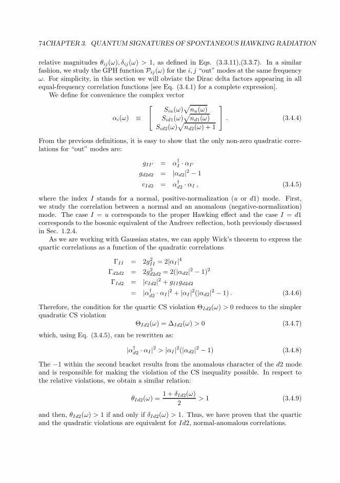
74CHAPTER 3. QUANTUM SIGNATURES OF SPONTANEOUS HAWKING RADIATION
relative magnitudes θij(ω), δij(ω) > 1, as defined in Eqs. (3.3.11),(3.3.7). In a similarfashion, we study the GPH function Pij(ω) for the i, j “out” modes at the same frequencyω. For simplicity, in this section we will obviate the Dirac delta factors appearing in allequal-frequency correlation functions [see Eq. (3.4.1) for a complete expression].
We define for convenience the complex vector
αi(ω) ≡
Siu(ω)√
nu(ω)
Sid1(ω)√
nd1(ω)
Sid2(ω)√
nd2(ω) + 1
. (3.4.4)
From the previous definitions, it is easy to show that the only non-zero quadratic corre-lations for “out” modes are:
gII′ = α†I · αI′
gd2d2 = |αd2|2 − 1
cId2 = α†d2 · αI , (3.4.5)
where the index I stands for a normal, positive-normalization (u or d1) mode. First,we study the correlation between a normal and an anomalous (negative-normalization)mode. The case I = u corresponds to the proper Hawking effect and the case I = d1corresponds to the bosonic equivalent of the Andreev reflection, both previously discussedin Sec. 1.2.4.
As we are working with Gaussian states, we can apply Wick’s theorem to express thequartic correlations as a function of the quadratic correlations
ΓII = 2g2II = 2|αI |4
Γd2d2 = 2g2d2d2 = 2(|αd2|2 − 1)2
ΓId2 = |cId2|2 + gIIgd2d2
= |α†d2 · αI |2 + |αI |2(|αd2|2 − 1) . (3.4.6)
Therefore, the condition for the quartic CS violation ΘId2(ω) > 0 reduces to the simplerquadratic CS violation
ΘId2(ω) = ∆Id2(ω) > 0 (3.4.7)
which, using Eq. (3.4.5), can be rewritten as:
|α†d2 · αI |2 > |αI |2(|αd2|2 − 1) (3.4.8)
The −1 within the second bracket results from the anomalous character of the d2 modeand is responsible for making the violation of the CS inequality possible. In respect tothe relative violations, we obtain a similar relation:
θId2(ω) =1 + δId2(ω)
2> 1 (3.4.9)
and then, θId2(ω) > 1 if and only if δId2(ω) > 1. Thus, we have proven that the quarticand the quadratic violations are equivalent for Id2, normal-anomalous correlations.
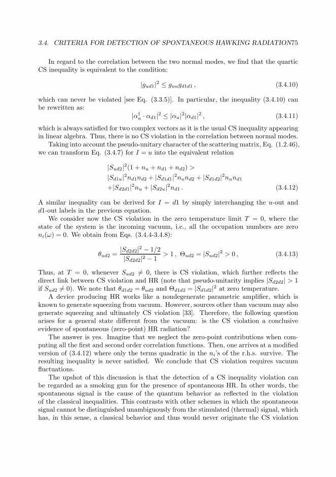
3.4. CRITERIA FOR DETECTION OF SPONTANEOUS HAWKING RADIATION75
In regard to the correlation between the two normal modes, we find that the quarticCS inequality is equivalent to the condition:
|gud1|2 ≤ guugd1d1 , (3.4.10)
which can never be violated [see Eq. (3.3.5)]. In particular, the inequality (3.4.10) canbe rewritten as:
|α†u · αd1|2 ≤ |αu|2|αd1|2 , (3.4.11)
which is always satisfied for two complex vectors as it is the usual CS inequality appearingin linear algebra. Thus, there is no CS violation in the correlation between normal modes.
Taking into account the pseudo-unitary character of the scattering matrix, Eq. (1.2.46),we can transform Eq. (3.4.7) for I = u into the equivalent relation
|Sud2|2(1 + nu + nd1 + nd2) >
|Sd1u|2nd1nd2 + |Sd1d1|2nund2 + |Sd1d2|2nund1
+|Sd2d1|2nu + |Sd2u|2nd1 . (3.4.12)
A similar inequality can be derived for I = d1 by simply interchanging the u-out andd1-out labels in the previous equation.
We consider now the CS violation in the zero temperature limit T = 0, where thestate of the system is the incoming vacuum, i.e., all the occupation numbers are zeroni(ω) = 0. We obtain from Eqs. (3.4.4-3.4.8):
θud2 =|Sd2d2|2 − 1/2
|Sd2d2|2 − 1> 1 , Θud2 = |Sud2|2 > 0 , (3.4.13)
Thus, at T = 0, whenever Sud2 6= 0, there is CS violation, which further reflects thedirect link between CS violation and HR (note that pseudo-unitarity implies |Sd2d2| > 1if Sud2 6= 0). We note that θd1d2 = θud2 and Θd1d2 = |Sd1d2|2 at zero temperature.
A device producing HR works like a nondegenerate parametric amplifier, which isknown to generate squeezing from vacuum. However, sources other than vacuum may alsogenerate squeezing and ultimately CS violation [33]. Therefore, the following questionarises for a general state different from the vacuum: is the CS violation a conclusiveevidence of spontaneous (zero-point) HR radiation?
The answer is yes. Imagine that we neglect the zero-point contributions when com-puting all the first and second order correlation functions. Then, one arrives at a modifiedversion of (3.4.12) where only the terms quadratic in the ni’s of the r.h.s. survive. Theresulting inequality is never satisfied. We conclude that CS violation requires vacuumfluctuations.
The upshot of this discussion is that the detection of a CS inequality violation canbe regarded as a smoking gun for the presence of spontaneous HR. In other words, thespontaneous signal is the cause of the quantum behavior as reflected in the violationof the classical inequalities. This contrasts with other schemes in which the spontaneoussignal cannot be distinguished unambiguously from the stimulated (thermal) signal, whichhas, in this sense, a classical behavior and thus would never originate the CS violation

76CHAPTER 3. QUANTUM SIGNATURES OF SPONTANEOUS HAWKING RADIATION
by itself. The same reasoning applies to the small perturbations around the condensatewave function since they are coherent excitations.
Now we turn our attention to the GPH criterion. From Eq. (3.3.26) we compute theGPH function for the pair of modes Id2:
PId2(ω) = (gIIgd2d2 − |cId2|2)[(gII + 1)(gd2d2 + 1)− |cId2|2] (3.4.14)
= ∆Id2(ω)[(gII + 1)(gd2d2 + 1)− |cId2|2] .
As the second (square) bracket in the r.h.s. of Eq. (3.4.14) is always positive [seeEq. (3.3.6)], we conclude that PId2 < 0 if and only if Eq. (3.4.7) is satisfied. As thestate is Gaussian, the GPH criterion is equivalent to the entanglement of the state ρ.Therefore, quadratic and quartic CS violations are equivalent to entanglement. In thisway, from the theoretical point of view, we can focus on studying the simpler quadratic CSviolation since all the extracted conclusions apply to the GPH criterion and the quarticCS violation.
We note that the equivalence between condition (3.4.7) and entanglement was alreadypointed out in Ref. [63] but the connection with the CS violation criterion was notmade explicit. A similar result appeared in Ref. [80] on the equivalence between non-separability and CS violation when studying the correlation function at two differenttimes in fluids of light.
When considering the entanglement between the two normal modes, we have |gud1| >|cud1| = 0 and thus there is no entanglement [see Eq. (3.3.26) and the ensuing discussion].
From the previous results we conclude that, when considering Gaussian and incoherentstates [i.e., Gaussian states satisfying Eq. (3.4.1)], all the here considered criteria forcharacterizing the quantum character of the system become equivalent. This result isimportant since it unifies the work of Refs. [2, 64, 63].
3.4.2 Final remarks
We briefly discuss the differences that arise when removing some restrictions. If thestate is Gaussian but not incoherent in the incoming channels, the GPH criterion is stillequivalent to the non-separability of the system. On the other hand, under the sameassumption, the quadratic CS violation is no longer equivalent to the GPH criterion;rather, it is only a sufficient condition for it, as argued in Sec. 3.3.1. Consequently, theGPH criterion is a more powerful criterion than the quadratic CS violation to detectnonseparability (it can identify nonseparability in cases where the quadratic CS violationwould fail). However, when relaxing the requirement of incoherence, the quartic CSviolation becomes independent of the GPH criterion (see Sec. 3.3.2). Even when thesetwo conditions are independent, both of them require the system to be described by anon-classical Glauber-Sudarshan function, i.e., a Glauber-Sudarshan function that takesnegative values (see discussion in Sec. 3.2).
On the other hand, if the state of the system is not Gaussian but is incoherent in theincoming channels, the quartic CS violation is also independent of the entanglement. Thequadratic CS violation and the GPH criterion are still equivalent between them, but nolonger equivalent to the entanglement of the system.

3.5. EXPERIMENTAL DETECTION SCHEMES 77
Gaussian Incoherent CS4 CS2 GPHYes Yes • ⇔ GPH • ⇔ GPH • ⇔ NSYes No • indep. NS • ⇒ GPH • ⇔ NSNo Yes • indep. NS • ⇔ GPH • ⇒ NSNo No • indep. NS • ⇒ GPH • ⇒ NS
Table 3.1: Logical relations between the different criteria studied throughout this workin the various physical cases. The three rightmost entries in the upper row indicatethe different criteria for the identification of quantum behavior: CS2, CS4 stand forquadratic and quartic CS violations, respectively, while GPH stands for generalized Peres-Horodecki criterion; NS means non-separability. The two leftmost columns define thevarious physical cases here considered. By “incoherent” state, we understand a densitymatrix which is diagonal in the representation of retarded quasiparticle scattering modes,each characterized by a single incoming channel; see Eq. (3.4.1). The symbol • stands forthe uppermost entry in the corresponding column. The abbreviation “indep.” means that,in the three lower cases, the quartic CS violation is independent of the non-separabilityof the system.
For a general state which does not satisfy any of the previous conditions, the quadraticCS violation is only a sufficient condition for the GPH criterion, which in turn is a sufficientcondition for the presence of entanglement. We summarize all these logical relations inTable 3.1.
Remarkably, the quadratic CS violation reveals at the same time two different aspectsof quantum behavior: the violation of a classical inequality and the entanglement of thesystem.
3.5 Experimental detection schemes
In this section, we discuss the possible experimental implementation of the previous cri-teria. A particular type of CS violation between two colliding condensates was measuredusing time-of-flight (TOF) detection [74]. Not long ago, a new proposal of detecting spon-taneous HR through TOF measurement of the phonon signal has been published [81]. Onthe other hand, the detection of entanglement using the GPH criterion was analyzed inRef. [64] considering density fluctuations or the optomechanical detection of phonons.Recently, it has been proposed that the entanglement of Hawking radiation in a BECcan be detected experimentally by measuring the density-density correlations through insitu imaging [65]. Following these works, we consider two detection schemes to detectspontaneous HR: TOF experiments and density-density correlations. All the results pre-sented in this section can be straightforwardly translated to study the Andreev reflectioninvolving d1, d2 modes. For the calculations, apart from stationarity and “Gaussianity”,we do not make any particular assumption on the form of the state of the system, ρ.

78CHAPTER 3. QUANTUM SIGNATURES OF SPONTANEOUS HAWKING RADIATION
3.5.1 Correlation between phonon and atomic time-of-flight sig-
nals.
In this specific detection scheme, we aim at detecting CS violation not in the phononsignal but rather in the atomic signal observed in a TOF experiment. We start byconsidering the atomic wave vectors involved for a given laboratory phonon frequencyω > 0, pu(ω) ≡ qu + ku−out(ω), pd2(ω) ≡ qd − kd2−out(ω), with qr the momentum of thewave function in the asymptotic homogeneous regions r = u, d. We require the atomicwave vectors from the upstream (downstream) region to be negative (positive), i.e., wejust consider frequencies where
pu(ω) < 0 (3.5.1)
[note that pd2(ω) > 0 is always verified for ω < ωmax since kd2−out(ωmax) < qd]. If all theseconditions are fulfilled, then there is no contribution from the condensate wave functionto the atomic signals and the corresponding wave packets travel in opposite directionswithout mixing. We suppose that the signals from the upstream and downstream regionscan be experimentally isolated.
We define the atom destruction operators localized in the asymptotic regions r as
cr (p) ≡∫
dx Ψ(x)f∗r (x) e−ipxe−iθr (3.5.2)
where we include the asymptotic phase of the condensate θr in order to get rid of it inthe resulting expressions. In the previous definition, the functions fr (x) are normalizedfunctions (
∫
dx|fr(x)|2 = 1) localized only in the corresponding asymptotic regions andtheir Fourier transforms are fr(k) =
1√2π
∫
dx e−ikxfr (x). They represent the envelope
of the Fourier transform, which has to be introduced to explicitly take into account thefact that the asymptotic subsonic and supersonic regions are placed in different spatialregions in a realistic situation. For simplicity, we assume that they are of the form
fr(x) =1√Lr
f
(
x− xrLr
)
, (3.5.3)
where f is a symmetric and real dimensionless function. We assume that Lr are sufficientlylarge for fr(k) to be well peaked at zero momentum. In this particular scenario of TOFdetection, we can understand fr(x) as the envelopes arising from the finite size, Lr, ofthe asymptotic regions and xr as the points in which they are centered. In the following,we assume that the size of the scattering region is much smaller than the size of theasymptotic regions. This implies that xu < 0 and xd > 0 and that:
xdLd
≃ − xuLu
≃ 1/2. (3.5.4)
3.5. EXPERIMENTAL DETECTION SCHEMES 79
Using Eq. (1.2.45) and following Eq. (1.2.43), we obtain the atomic operators:
cu (pu (ω)) ≃∫
dω′ f∗u(ku−out(ω
′)− ku−out(ω))uu−out(ω
′)
|wu−out (ω′)|1/2γu−out(ω
′)
+ f∗u(−ku−in(ω
′)− ku−out(ω))v∗u−in(ω
′)
|wu−in (ω′) |1/2 γ†u−in(ω
′) (3.5.5)
cd (pd2 (ω)) ≃∫ ωmax
0
dω′ f∗d (kd2−out(ω)− kd2−out(ω
′))v∗d2−out(ω
′)
|wd2−out (ω′) |1/2 γd2−out(ω′)
+
∫
dω′ f∗d (kd2−out(ω)− kd1−out(ω
′))v∗d1−out(ω
′)
|wd1−out (ω′) |1/2 γ†d1−out(ω
′),
We can now compute the corresponding atomic first-order correlation functions, namely,
〈c†u (pu (ω)) cu (pu (ω))〉 = |uu−out(ω)|2|αu(ω)|2 + |vu−in(ωuu(ω))|2[1 + nu(ωuu(ω))]
〈c†d (pd2 (ω)) cd (pd2 (ω))〉 = |vd2−out(ω)|2[|αd2(ω)|2 − 1] (3.5.6)
+ |vd1−out(ωd1d2(ω))|2[|αd1(ωd1d2(ω))|2 + 1]
〈cd (pd2 (ω)) cu (pu (ω))〉 = [α†d2(ω) · αu(ω)]uu−out(ω)v
∗d2−out(ω)F (ω),
where ωd1d2(ω) = ωd1(kd2−out(ω)) and ωuu(ω) = ωu(−ku−out(ω)), with ωi(k) the dis-persion relation of scattering channel i (see Fig. 3.1). We see that the terms related tothe direct phonon signal are weighted with the dominant component of the BdG spinor(remember that for the d2 modes, vd2−out > ud2−out as they are anomalous) while thecontribution related to the depletion cloud is weighted by the minor component of theBdG spinor.
The overlap function in the last line of Eq. (3.5.6) is:
F (ω) =
∫
dk f∗u
(
k
ζ(ω)
)
f∗d (kζ(ω)) (3.5.7)
=1√LuLd
∫
dx f∗(
ζ (ω)x+ xuLu
)
f∗(
ζ (ω)−1x− xd
Ld
)
,
with
ζ(ω) ≡∣
∣
∣
∣
wu−out(ω)
wd2−out(ω)
∣
∣
∣
∣
1/2
. (3.5.8)
From a mathematical point of view, the integral F (ω) can be regarded as the scalarproduct of two normalized functions, hence F (ω) ≤ 1. Taking into account Eq. (3.5.4)and that the f function is normalized, it easy to show that this inequality saturates forω0 such that
ζ(ω0) =
√
Lu
Ld(3.5.9)
The previous condition has a straightforward physical interpretation. The phonon op-erators are evaluated in the frequency domain. The frequency resolution near a givenfrequency ω0 for both wave packets is given by
∆ωu−out/d2−out(ω0) = |wu−out/d2−out (ω0) |∆ku/d. (3.5.10)
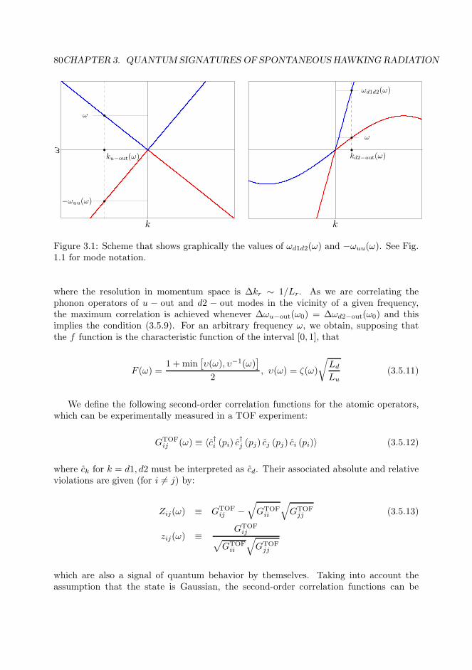
80CHAPTER 3. QUANTUM SIGNATURES OF SPONTANEOUS HAWKING RADIATION
k
ω
ω
ku−out(ω)
−ωuu(ω)
k
ω
ωd1d2(ω)
kd2−out(ω)
Figure 3.1: Scheme that shows graphically the values of ωd1d2(ω) and −ωuu(ω). See Fig.1.1 for mode notation.
where the resolution in momentum space is ∆kr ∼ 1/Lr. As we are correlating thephonon operators of u − out and d2 − out modes in the vicinity of a given frequency,the maximum correlation is achieved whenever ∆ωu−out(ω0) = ∆ωd2−out(ω0) and thisimplies the condition (3.5.9). For an arbitrary frequency ω, we obtain, supposing thatthe f function is the characteristic function of the interval [0, 1], that
F (ω) =1 +min
[
υ(ω), υ−1(ω)]
2, υ(ω) = ζ(ω)
√
Ld
Lu(3.5.11)
We define the following second-order correlation functions for the atomic operators,which can be experimentally measured in a TOF experiment:
GTOFij (ω) ≡ 〈c†i (pi) c
†j (pj) cj (pj) ci (pi)〉 (3.5.12)
where ck for k = d1, d2 must be interpreted as cd. Their associated absolute and relativeviolations are given (for i 6= j) by:
Zij(ω) ≡ GTOFij −
√
GTOFii
√
GTOFjj (3.5.13)
zij(ω) ≡GTOF
ij√
GTOFii
√
GTOFjj
which are also a signal of quantum behavior by themselves. Taking into account theassumption that the state is Gaussian, the second-order correlation functions can be

3.5. EXPERIMENTAL DETECTION SCHEMES 81
expressed, using Wick’s theorem, in terms of the first-order correlation functions as
GTOFuu (ω) = 〈c†u (pu) c†u (pu) cu (pu) cu (pu)〉
= 2| 〈c†u (pu) cu (pu)〉 |2
GTOFd2d2 (ω) = 〈c†d (pd2) c
†d (pd2) cd (pd2) cd (pd2)〉
= 2| 〈c†d (pd2) cd (pd2)〉 |2 (3.5.14)
GTOFud2 (ω) = 〈c†d (pd2) c†u (pu) cd (pd2) cu (pu)〉
= 〈c†d (pd2) c†u (pu)〉 〈cd (pd2) cu (pu)〉+ 〈c†d (pd2) cd (pd2)〉 〈c†u (pu) cu (pu)〉 .
By comparing Eqs. (3.5.6) and (3.5.14) with Eq. (3.4.5), one can infer that zud2 > 1implies δud2 > 1, i.e., that the quartic atom CS violation is a sufficient condition for thequadratic CS violation in the phonon signal.
We see that in Eq. (3.5.14) the crossed correlations of the type 〈cu (pu (ω)) cu (pu (ω))〉,〈cd (pd2) cd (pd2)〉, 〈c†u (pu (ω)) cd (pd2)〉 and so on vanish. This is of course true for anincoming incoherent state since in that case they are identically zero. Interestingly, thisresult also holds for a general state but for a very different reason: for those correlations,the appearing overlap integrals, similar to F (ω), give zero. We refer to the end of Sec.3.5.2 for the complete explanation of this phenomenon.
3.5.2 Density-density correlations
The role of the spatial density correlation function in analog models has been extensivelystudied in several works [15, 31, 23]. In the BEC context, the measurement of the spatialdensity correlations has been experimentally used to characterize the BH laser [21]. Thedensity-density correlation function also plays an important role in the polariton analog[36, 12].
We start our analysis by considering the density in the BdG approximation of Sec.1.2 and expanding it up to first order in the fluctuations of the field operator
n(x) = Ψ†(x)Ψ(x) ≃ n(x) + δn(x), δn(x) = Ψ∗0(x)ϕ(x) + Ψ0(x)ϕ
†(x) (3.5.15)
and n(x) = |Ψ0(x)|2 the usual mean-field density. The expression for the density fluc-tuations is formally similar to that of ϕ(x), see Eq. (1.2.45). Importantly, the densityfluctuation operator δn(x) in the BdG approximation is linear in the destruction opera-tors, rather than quadratic. Thus, we can extract the quadratic correlations of Sec. 3.3by measuring density-density correlations [64, 65]. For that purpose, we restrict ourselvesto the asymptotic (subsonic and supersonic) regions. By taking the Fourier transform ofthe density in the asymptotic regions at k 6= 0, we can get rid of the condensate signaland extract the phonon signal. Analogously to Eq. (3.5.2), we define:
nr (k) ≡∫
dx n(x)f∗r (x) e−ikx , (3.5.16)
with fr (x) as given in Eq. (3.5.3). However, in this case, the envelope has a differ-ent physical explanation. In a TOF experiment, we only have access to the signal in
82CHAPTER 3. QUANTUM SIGNATURES OF SPONTANEOUS HAWKING RADIATION
momentum space and thus, the envelopes arise from the finite size of the asymptoticregions. Using in situ imaging [82, 65], we have direct access to the density in real spaceso the envelopes fr (x) can be appropriately selected to extract the corresponding Fouriertransforms. In particular, this implies that we can choose freely the values of xu,d, Lu,d,in contrast to the situation of TOF detection, where they were fixed by the size of theasymptotic regions, see Eq. (3.5.4) and related discussion.
Taking into account all the previous considerations, we obtain:
nu (ku−out(ω)) ≃ √nu
[
∫
dω′ f∗u(ku−out(ω
′)− ku−out(ω))ru−out(ω
′)
|wu−out (ω′)|1/2γu−out(ω
′)
+ f∗u(−ku−in(ω
′)− ku−out(ω))ru−in(ω
′)
|wu−in (ω′) |1/2 γ†u−in(ω
′)
]
(3.5.17)
nd (−kd2−out(ω)) ≃ √nd
∫ ωmax
0
dω′ f∗d (kd2−out(ω)− kd2−out(ω
′))rd2−out(ω
′)
|wd2−out (ω′) |1/2 γd2−out(ω′)
+√nd
∫
dω′ f∗d (kd2−out(ω)− kd1−out(ω
′))rd1−out(ω
′)
|wd1−out (ω′) |1/2 γ†d1−out(ω
′),
where ra(ω) is [see Eq. (1.2.42)]
ra(ω) = ua(ω) + va(ω) =
√
k2a2Ωa(ω)
, (3.5.18)
and we have used |ω − vrka(ω)| = Ωa(ω) =√
c2rk2 + k4
4 . It is worth noting that, if we
leave freedom to choose the values of xu,d, Lu,d in the envelopes of the atomic operatorsof Eq. (3.5.2), we find:
nr(k) =√nr[cr(qr + k) + c†r(−qr − k)] (3.5.19)
where nr is the density in the asymptotic region r. Now, we can connect the correlationsstudied in Sec. 3.3 with the density correlations by taking into account that n†
r(k) =nr(−k). We obtain:
Guu(ω) ≡ 〈nu (−ku−out (ω)) nu (ku−out (ω))〉 = nur2u−out(ω)[guu(ω) + nu(ωuu(ω)) + 1]
Gd2d2(ω) ≡ 〈nd (kd2−out(ω)) nd (−kd2−out(ω))〉 = ndr2d2−out(ω)[gd2d2(ω) + gd1d1(ωd1d2(ω)) + 1]
Gud2(ω) ≡ 〈nd (−kd2−out(ω)) nu (ku−out (ω))〉 = F (ω)√nundru−outrd2−outcud2(ω) , (3.5.20)
with ωd1d2(ω) and ωuu(ω) defined after Eq. (3.5.6) and F (ω) given by Eq. (3.5.25). Wenote the strong analogy of the previous equation with its TOF equivalent (3.5.6), whichresults from the formal analogy between the expressions for the density fluctuations andthe field operator fluctuations, compare for instance Eqs. (3.5.5) and (3.5.17).
Similar to the TOF case, it is easy to prove that F (ω) = 1 when
ζ(ω) =
√
Lu
Ld=
√
∣
∣
∣
∣
xuxd
∣
∣
∣
∣
, (3.5.21)

3.5. EXPERIMENTAL DETECTION SCHEMES 83
We have extended the condition (3.5.9) to all frequencies ω since Lu,d2, xu,d are nowfree parameters and we can vary them to fulfill the previous relation for each value ofthe frequency. This condition has been interpreted in the case of TOF detection as thecondition for the wave-packets to have equal width in frequency space. However, resultingfrom the well-known properties of the spatial density correlations, Eq. (3.5.21) can be alsointerpreted as expressing that the wave packets in the subsonic and supersonic regionshave to be placed along the correlation lines that maximize the spatial density correlationfunction, see Refs. [15, 31, 23]. In the following, we take F (ω) = 1.
It is worth noting that the correlation functions Gij(ω) can never violate the CSinequality by themselves since Gud2 <
√GuuGd2d2. This is due to the fact that now the
depletion cloud contribution is weighted with the same coefficient as the direct phononsignal, in contrast to the atomic correlations of the TOF case, see discussion after Eq.(3.5.6).
In order to get over this problem, we try to relate these functions, which can bemeasured, to the phonon correlations. For that purpose, we introduce the normalizeddensity-density correlations:
Gij(ω) ≡Gij(ω)√
ninjri−out(ω)rj−out, (3.5.22)
From Eq. (3.5.20), we see that Gud2(ω) = cud2(ω). For extracting the other correlations,in a similar way to Ref. [65] we define the magnitudes:
guu(ω) ≡ guu(ω) + nu(ωuu(ω)) = Guu(ω)− 1
gd2d2(ω) ≡ gd2d2(ω) + gd1d1(ωd1d2(ω)) = Gd2d2(ω)− 1
(3.5.23)
The −1 appearing in the definitions of guu(ω), gd2d2(ω) reflects the subtraction of theatomic depletion contribution.
We see that the functions guu, gd2d2 are over-estimations of correlations guu, gd2d2,since nu, gd1d1 are always positive. From this, we can define the quantity:
∆ud2 ≡ |cud2|2 − guugd2d2 , (3.5.24)
noting that ∆ud2 > ∆ud2. Thus, measuring ∆ud2 > 0 amounts to experimentally observ-ing the quadratic CS violation, in a close analogy to case of TOF detection, where themeasurement of CS violation in the atomic signal implies the quadratic CS violation. Weremark that, for these calculations, we have only assumed that the state of the system isstationary and here, we do not even have assumed Gaussian behavior as it was done inthe TOF scheme.
The upshot of this discussion is that we can observe the violation of a quadratic CS in-equality through the measurement of the function ∆ud2. Similar claims can be made aboutthe measurement of the quadratic CS inequality involving the d1, d2 modes, where we canrepeat the same strategy of above to obtain the correlation functions gd1d1, cd1d2. However,it is not possible to obtain the correlation functions cuu, cd1d1, cd2d2, gud2, gd1d2 from thisscheme. This is due to the vanishing overlap integrals that appear when trying to obtain
84CHAPTER 3. QUANTUM SIGNATURES OF SPONTANEOUS HAWKING RADIATION
the corresponding correlations. For instance, if we compute 〈nu (ku−out (ω)) nu (ku−out (ω))〉,we face an overlap integral of the type
∫
dk f∗u (k) f∗
u (k) =
∫
dx f∗u (x) f∗
u (−x) = 0, (3.5.25)
because the fu function is, by construction, well localized in the subsonic region, far fromthe scattering region around x = 0, see Eq. (3.5.16) and the discussion below. Thus, wecannot obtain cuu by this method. A similar reasoning applies to other correlations.
It is important to note the crucial role played by the spatial location of the asymptoticregions. If we do not take into account the spatial location by introducing the envelopesin Eq. (3.5.16) and we take the Fourier transforms as ideally infinite, we would obtain:
nu (ku−out(ω)) ≃√nu × (3.5.26)
×(
ru−out(ω)
|wu−out (ω)|1/2γu−out(ω) +
ru−in(ωuu(ω))
|wu−in (ωuu(ω)) |1/2γ†u−in(ωuu(ω))
)
nd (−kd2−out(ω)) ≃√nd ×
×(
rd2−out(ω)
|wd2−out (ω) |1/2γd2−out(ω) +
rd1−out(ωd1d2(ω))
|wd1−out (ωd1d2(ω)) |1/2γ†d1−out(ωd1d2(ω))
)
,
This assumption would lead to contradictory results. For instance, the commutator
[nu (ku−out(ω)) , nu (−ku−in(ω))] = nuru−out(ω)
|wu−out (ω)|1/2ru−in(ω)
|wu−in (ω) |1/2Suu(ω) 6= 0
(3.5.27)is non-vanishing but it should be zero as [n(x), n(x′)] = 0 for every x, x′. However, whenusing the full expressions of Eq. (3.5.17) we arrive at the correct result
[nu (ku−out(ω)) , nu (−ku−in(ω))] = nuru−out(ω)
|wu−out (ω)|1/2ru−in(ω)
|wu−in (ω) |1/2× (3.5.28)
× Suu(ω)
∫
dω′ f∗u
(
− ω′ − ω
|wu−in (ω) |
)
f∗u
(
− ω′ − ω
|wu−out (ω) |
)
The integral of the r.h.s, after turning back to real space, is similar to that consideredin Eq. (3.5.25) and gives zero.
We arrive at the same conclusion when considering the density-density correlationsin real space. As noted in Ref. [31], only the terms with a stationary phase should bekept when computing 〈n(x)n(x′)〉, which yields the condition (3.5.21). In particular, onlythe “proper” correlations between out-out modes can be extracted cud2, cd1d2, gud1. Theother correlations cuu, cd1d1, cd2d2, gud2, gd1d2, cud1, even when they are non-zero, cannotbe obtained because the associated exponential terms do not present a stationary phasewhen integrating over frequencies.
Thus, an important consequence of taking into account the spatial location of thesubsonic and supersonic regions is the conclusion that only a limited number of correla-tions can be experimentally observed. In particular, this implies that we cannot measure

3.6. NUMERICAL RESULTS 85
all the correlation functions appearing in the GPH criterion (3.3.23). Moreover, and forthe same reason, if the state is Gaussian, we cannot obtain all the correlation functionsappearing in the quartic CS violation, see Eq. (3.3.30). The results here presented showthat we can only aim at observing a quadratic CS violation within this kind of detectionschemes. A similar claim can be maid about the TOF detection scheme here presented,where we can only observe indirectly the quadratic CS violation and we can never extractthe full GPH criterion from the measurements. We can expect that this phenomenon isnot exclusive of these specific procedures. Any realistic attempt to obtain the correlationfunctions between phonons has to take necessarily into account the spatial location of theasymptotic regions and thus, similar reasonings would arise.
Nevertheless, the previous considerations do not pose a problem for the detection ofthe quantum Hawking effect for two reasons: (a) if the state of the system is incoherentover the incoming channels, we have proven that the GPH criterion and the quartic CSviolation are equivalent to the quadratic CS violation and (b) even for an arbitrary statein which the previous relations do not hold, the quadratic CS violation is still a signatureof the presence of the entanglement; in particular, it is a sufficient condition for thefulfillment of the GPH criterion. More than that, as remarked at the end of Sec. 3.3, thequadratic CS violation is also by itself a clear indication of the quantum nature of thesystem, as CS inequalities are always satisfied in a classical system.
3.6 Numerical results
Here, we compute numerically the different correlation functions and the associatedphonon CS violation. We also compute the experimental magnitudes corresponding to thedifferent detection schemes. For definiteness, we consider the usual case where the stateof the system is given by a thermal distribution over the incoming modes, Eq. (3.4.2). Forthis class of states, all the discussed criteria become equivalent, as argued before. Sincewe only aim at the identification of some physical trends and not at the study of thewhole parameter space, characterized by 7 variables (see Appendix G), we study the CSviolation using the BH configurations presented in Sec. 1.3. For simplifying the results,we set units such ~ = m = cu = kB = 1, cu being the upstream sound speed.
First, we make some general theoretical remarks before showing the numerical results.In the conventional (ω = 0) peak of the Hawking spectrum |Sud2(ω)|2, the scatteringmatrix elements diverge as |Sij(ω)| ∼ 1/
√ω with i arbitrary and j = d1, d2 . By contrast,
Siu(ω) in the same limit (ω → 0+) saturates to a nonzero constant (the asymptoticbehavior of the S−matrix coefficients is discussed in Appendix C). On the other hand,the only occupation factor which diverges is nu(ω) ∼ 1/ω, because Ωu(ω) is the onlycomoving frequency that vanishes for small ω. From pseudo-unitarity it follows that|Sud2|2 − |Sd2d1|2 = |Sd2u|2 − |Sd1d2|2. We then conclude from Eq. (3.4.12) that there isno CS violation in the ω → 0+ region. This argument relies solely on the presence of auniform condensate flow connecting the subsonic and supersonic asymptotic regions, andnot on other details of the scattering structure.
In the opposite frequency region, ω → ω−max, it is easy to show from the results of
Appendix C that θud2(ω) = 1/2 + O (√ωmax − ω). This leaves us with only the central
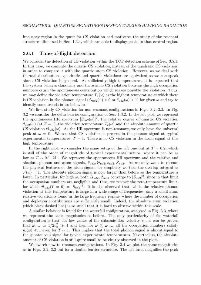
86CHAPTER 3. QUANTUM SIGNATURES OF SPONTANEOUS HAWKING RADIATION
frequency region in the quest for CS violation and motivates the study of the resonantstructures discussed in Sec. 1.3.4, which are able to display peaks in that central region.
3.6.1 Time-of-flight detection
We consider the detection of CS violation within the TOF detection scheme of Sec. 3.5.1.In this case, we compute the quartic CS violation, instead of the quadratic CS violation,in order to compare it with the quartic atom CS violation. However, as we deal withthermal distributions, quadratic and quartic violations are equivalent so we can speakabout CS violation in general. At sufficiently high temperatures, it is expected thatthe system behaves classically and there is no CS violation because the high occupationnumbers crush the spontaneous contribution which makes possible the violation. Thus,we may define the violation temperature Tv(ω) as the highest temperature at which thereis CS violation in the phonon signal (∆ud2(ω) > 0 or δud2(ω) > 1) for given ω and try toidentify some trends in its behavior.
We first study CS violation for non-resonant configurations in Figs. 3.2, 3.3. In Fig.3.2 we consider the delta-barrier configuration of Sec. 1.3.2. In the left plot, we representthe spontaneous HR spectrum |Sud2(ω)|2, the relative degree of quartic CS violationθud2(ω) (at T = 1), the violation temperature Tv(ω) and the absolute amount of quarticCS violation Θud2(ω). As the HR spectrum is non-resonant, we only have the universalpeak at ω = 0. We see that CS violation is present in the phonon signal at typicalexperimental temperatures, T = 1. There is no CS violation in the atom signal at thishigh temperature.
In the right plot, we consider the same setup of the left one but at T = 0.2, whichis still of the order of magnitude of typical experimental setups, where it can be aslow as T ∼ 0.1 [21]. We represent the spontaneous HR spectrum and the relative andabsolute phonon and atom signals, θud2,Θud2, zud2, Zud2. As we only want to discussthe physical features of the atom signal, for simplicity we take the overlap integral asF (ω) = 1. The absolute phonon signal is now larger than before as the temperature islower. In particular, for high ω, both ∆ud2, ∆ud2 converge to |Sud2|2, since in that limitthe occupation numbers are negligible and thus, we recover the zero-temperature limit,for which Θud2(T = 0) = |Sud2|2. It is also observed that, while the relative phononviolation at this temperature is large in a wide range of frequencies, only a small atomrelative violation is found in the large frequency regime, where the number of occupationand depletion contributions are sufficiently small. Indeed, the absolute atom violation(thick black dashed line) is so small that it is hard to observe within this scale.
A similar behavior is found for the waterfall configuration, analyzed in Fig. 3.3, wherewe represent the same magnitudes as before. The only particularity of the waterfallconfiguration is that, for low values of the subsonic flow velocity vu, it can be proventhat ωmax ≃ 1/2v2u ≫ 1 and then for ω . ωmax all the occupation numbers satisfyni(ω) ≪ 1 even for T ∼ 1. This implies that the total phonon signal is almost equal tothe spontaneous signal for typical experimental temperatures. Nevertheless, the absoluteamount of CS violation is still quite small to be clearly observed in the plots.
We switch now to resonant configurations. In Fig. 3.4 we plot the same magnitudesas in Figs. 3.2, 3.3 but for a double barrier structure. The left inset magnifies the peak
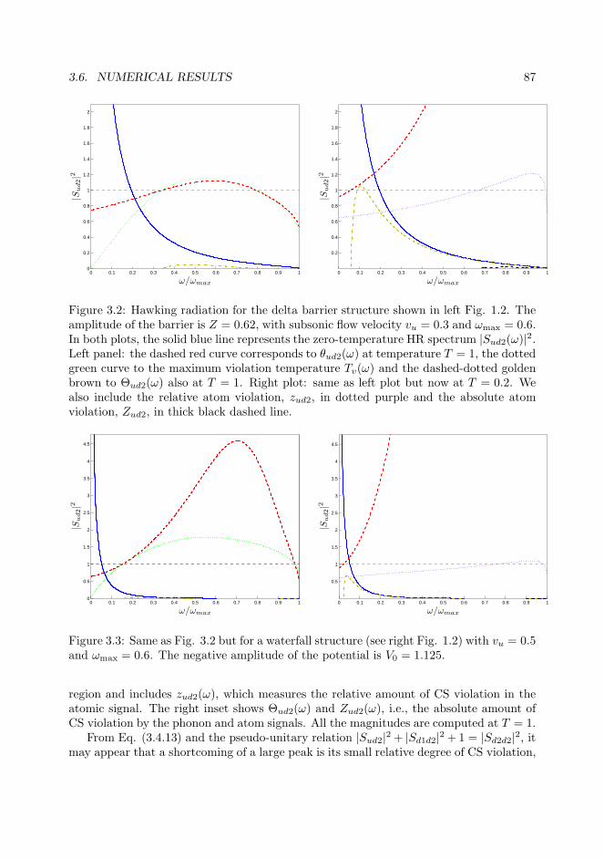
3.6. NUMERICAL RESULTS 87
0 0.1 0.2 0.3 0.4 0.5 0.6 0.7 0.8 0.9 10
0.2
0.4
0.6
0.8
1
1.2
1.4
1.6
1.8
2
ω/ωmax
|Su
d2|2
0 0.1 0.2 0.3 0.4 0.5 0.6 0.7 0.8 0.9 1
0.2
0.4
0.6
0.8
1
1.2
1.4
1.6
1.8
2
ω/ωmax
|Su
d2|2
Figure 3.2: Hawking radiation for the delta barrier structure shown in left Fig. 1.2. Theamplitude of the barrier is Z = 0.62, with subsonic flow velocity vu = 0.3 and ωmax = 0.6.In both plots, the solid blue line represents the zero-temperature HR spectrum |Sud2(ω)|2.Left panel: the dashed red curve corresponds to θud2(ω) at temperature T = 1, the dottedgreen curve to the maximum violation temperature Tv(ω) and the dashed-dotted goldenbrown to Θud2(ω) also at T = 1. Right plot: same as left plot but now at T = 0.2. Wealso include the relative atom violation, zud2, in dotted purple and the absolute atomviolation, Zud2, in thick black dashed line.
0 0.1 0.2 0.3 0.4 0.5 0.6 0.7 0.8 0.9 10
0.5
1
1.5
2
2.5
3
3.5
4
4.5
ω/ωmax
|Su
d2|2
0 0.1 0.2 0.3 0.4 0.5 0.6 0.7 0.8 0.9 1
0.5
1
1.5
2
2.5
3
3.5
4
4.5
ω/ωmax
|Su
d2|2
Figure 3.3: Same as Fig. 3.2 but for a waterfall structure (see right Fig. 1.2) with vu = 0.5and ωmax = 0.6. The negative amplitude of the potential is V0 = 1.125.
region and includes zud2(ω), which measures the relative amount of CS violation in theatomic signal. The right inset shows Θud2(ω) and Zud2(ω), i.e., the absolute amount ofCS violation by the phonon and atom signals. All the magnitudes are computed at T = 1.
From Eq. (3.4.13) and the pseudo-unitary relation |Sud2|2 + |Sd1d2|2 +1 = |Sd2d2|2, itmay appear that a shortcoming of a large peak is its small relative degree of CS violation,
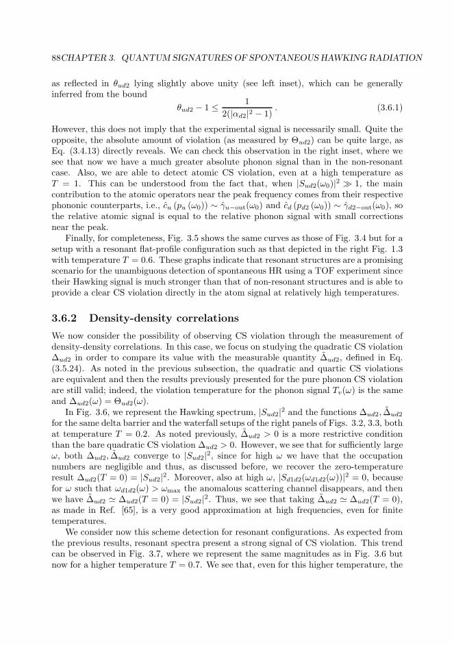
88CHAPTER 3. QUANTUM SIGNATURES OF SPONTANEOUS HAWKING RADIATION
as reflected in θud2 lying slightly above unity (see left inset), which can be generallyinferred from the bound
θud2 − 1 ≤ 1
2(|αd2|2 − 1). (3.6.1)
However, this does not imply that the experimental signal is necessarily small. Quite theopposite, the absolute amount of violation (as measured by Θud2) can be quite large, asEq. (3.4.13) directly reveals. We can check this observation in the right inset, where wesee that now we have a much greater absolute phonon signal than in the non-resonantcase. Also, we are able to detect atomic CS violation, even at a high temperature asT = 1. This can be understood from the fact that, when |Sud2(ω0)|2 ≫ 1, the maincontribution to the atomic operators near the peak frequency comes from their respectivephononic counterparts, i.e., cu (pu (ω0)) ∼ γu−out(ω0) and cd (pd2 (ω0)) ∼ γd2−out(ω0), sothe relative atomic signal is equal to the relative phonon signal with small correctionsnear the peak.
Finally, for completeness, Fig. 3.5 shows the same curves as those of Fig. 3.4 but for asetup with a resonant flat-profile configuration such as that depicted in the right Fig. 1.3with temperature T = 0.6. These graphs indicate that resonant structures are a promisingscenario for the unambiguous detection of spontaneous HR using a TOF experiment sincetheir Hawking signal is much stronger than that of non-resonant structures and is able toprovide a clear CS violation directly in the atom signal at relatively high temperatures.
3.6.2 Density-density correlations
We now consider the possibility of observing CS violation through the measurement ofdensity-density correlations. In this case, we focus on studying the quadratic CS violation∆ud2 in order to compare its value with the measurable quantity ∆ud2, defined in Eq.(3.5.24). As noted in the previous subsection, the quadratic and quartic CS violationsare equivalent and then the results previously presented for the pure phonon CS violationare still valid; indeed, the violation temperature for the phonon signal Tv(ω) is the sameand ∆ud2(ω) = Θud2(ω).
In Fig. 3.6, we represent the Hawking spectrum, |Sud2|2 and the functions ∆ud2, ∆ud2
for the same delta barrier and the waterfall setups of the right panels of Figs. 3.2, 3.3, bothat temperature T = 0.2. As noted previously, ∆ud2 > 0 is a more restrictive conditionthan the bare quadratic CS violation ∆ud2 > 0. However, we see that for sufficiently largeω, both ∆ud2, ∆ud2 converge to |Sud2|2, since for high ω we have that the occupationnumbers are negligible and thus, as discussed before, we recover the zero-temperatureresult ∆ud2(T = 0) = |Sud2|2. Moreover, also at high ω, |Sd1d2(ωd1d2(ω))|2 = 0, becausefor ω such that ωd1d2(ω) > ωmax the anomalous scattering channel disappears, and thenwe have ∆ud2 ≃ ∆ud2(T = 0) = |Sud2|2. Thus, we see that taking ∆ud2 ≃ ∆ud2(T = 0),as made in Ref. [65], is a very good approximation at high frequencies, even for finitetemperatures.
We consider now this scheme detection for resonant configurations. As expected fromthe previous results, resonant spectra present a strong signal of CS violation. This trendcan be observed in Fig. 3.7, where we represent the same magnitudes as in Fig. 3.6 butnow for a higher temperature T = 0.7. We see that, even for this higher temperature, the
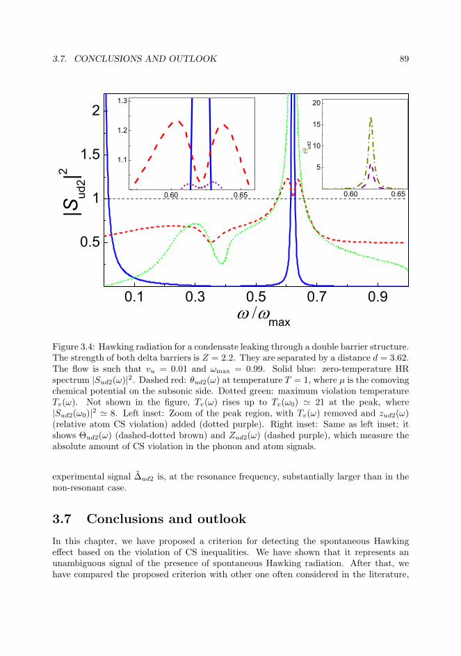
3.7. CONCLUSIONS AND OUTLOOK 89
0.1 0.3 0.5 0.7 0.9
0.5
1
1.5
2
|Sud
2|2
max
0.60 0.65
1.1
1.2
1.3
0.60 0.65
5
10
15
20
ud
2
Figure 3.4: Hawking radiation for a condensate leaking through a double barrier structure.The strength of both delta barriers is Z = 2.2. They are separated by a distance d = 3.62.The flow is such that vu = 0.01 and ωmax = 0.99. Solid blue: zero-temperature HRspectrum |Sud2(ω)|2. Dashed red: θud2(ω) at temperature T = 1, where µ is the comovingchemical potential on the subsonic side. Dotted green: maximum violation temperatureTv(ω). Not shown in the figure, Tv(ω) rises up to Tv(ω0) ≃ 21 at the peak, where|Sud2(ω0)|2 ≃ 8. Left inset: Zoom of the peak region, with Tv(ω) removed and zud2(ω)(relative atom CS violation) added (dotted purple). Right inset: Same as left inset; itshows Θud2(ω) (dashed-dotted brown) and Zud2(ω) (dashed purple), which measure theabsolute amount of CS violation in the phonon and atom signals.
experimental signal ∆ud2 is, at the resonance frequency, substantially larger than in thenon-resonant case.
3.7 Conclusions and outlook
In this chapter, we have proposed a criterion for detecting the spontaneous Hawkingeffect based on the violation of CS inequalities. We have shown that it represents anunambiguous signal of the presence of spontaneous Hawking radiation. After that, wehave compared the proposed criterion with other one often considered in the literature,

90CHAPTER 3. QUANTUM SIGNATURES OF SPONTANEOUS HAWKING RADIATION
0.1 0.3 0.5 0.7 0.9
1
2
3
4
max
|Sud
2|2
0.92 0.94 0.96 0.98
1.1
1.2
0.92 0.94 0.96 0.98
0.5
1
1.5
ud
2
Figure 3.5: Same as Fig. 3.4 but for T = 0.6 and for a resonant flat-profile structurewith two sharp variations in the local speed of sound, which takes the successive values1, 0.43, 0.6, as depicted in the right Fig. 1.3. The intermediate region has a length L = 26.The flow is such that qu = 0.95 and ωmax = 0.18.
the GPH criterion. In particular, we have shown that, under certain physical conditions(Gaussian processes and, simultaneously, incoherent incoming channels), all the consid-ered criteria are equivalent.
We have also investigated the possible measurement of the different criteria in exper-imental detection schemes. By taking into account the different spatial location of thesubsonic and supersonic regions, we have shown that only certain correlation functionscan be obtained. For simplicity we have focused on two specific detection schemes, butwe expect similar problems to arise in other kind of measurements, since in any realisticsituation the supersonic and subsonic regions are necessarily placed in different regions.However, our work also shows that this limitation is not a major problem, as we can oftenmeasure the quadratic CS violation, which is also a sufficient condition for the entangle-ment of the system. Finally, our numerical results of Sec. 3.6 show that, in typical analogconfigurations, the CS violation can be detected in an achievable range of temperatures.

3.7. CONCLUSIONS AND OUTLOOK 91
0.1 0.2 0.3 0.4 0.5 0.6 0.7 0.8 0.9
0.2
0.4
0.6
0.8
1
1.2
1.4
1.6
1.8
2
ω/ωmax
|Su
d2|2
|Sud2|2
∆ud2
∆ud2
0.1 0.2 0.3 0.4 0.5 0.6 0.7 0.8 0.9
0.1
0.2
0.3
0.4
0.5
0.6
0.7
0.8
0.9
1
ω/ωmax
|Su
d2|2
|Sud2|2
∆ud2
∆ud2
Figure 3.6: Plot of the Hawking radiation spectrum and the functions ∆ud2, ∆ud2 fora delta barrier configuration (left panel) and a waterfall configuration (right panel), attemperature T = 0.2. For the delta barrier, the subsonic flow speed is vu = 0.3 and thebarrier strength is Z = 0.62. For the waterfall setup, the subsonic flow speed is vu = 0.5and the potential depth is V0 = 1.125.
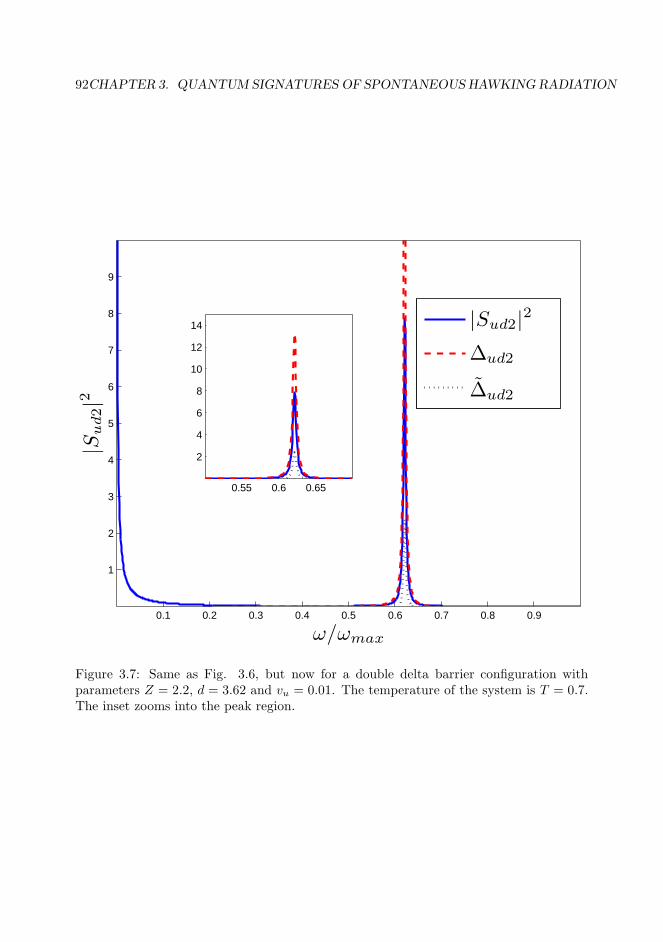
92CHAPTER 3. QUANTUM SIGNATURES OF SPONTANEOUS HAWKING RADIATION
0.1 0.2 0.3 0.4 0.5 0.6 0.7 0.8 0.9
1
2
3
4
5
6
7
8
9
ω/ωmax
|Su
d2|2
|Sud2|2
∆ud2
∆ud2
0.55 0.6 0.65
2
4
6
8
10
12
14
Figure 3.7: Same as Fig. 3.6, but now for a double delta barrier configuration withparameters Z = 2.2, d = 3.62 and vu = 0.01. The temperature of the system is T = 0.7.The inset zooms into the peak region.
Chapter 4Time-dependent study of a black-hole
laser in a flowing atomic condensate
4.1 Introduction
So far, we have focused on the emission of Hawking radiation by a single sonic black-hole.We now switch to a slightly different gravitational analog system: the so-called black-holelaser, formed by a pair of neighboring horizons and first discussed in the gravitationalcontext in Ref. [83]. Within this analog scenario, for a quantum Bose field with asuperluminal dispersion, the negative energy partner of the Hawking emission by theouter horizon can bounce on the inner horizon and travel back to the outer one, soto stimulate further Hawking emission. In suitable conditions, this process may giverise to a dynamical instability (similar to that arising in a laser system) and then tothe exponential growth of a self-amplifying coherent Hawking emission. This coherentemission contrasts with the spontaneous emission Hawking radiation from a single horizon,with unambiguously quantum features, as discussed in the previous chapter. The firstexperimental evidence of the BH laser instability has been recently reported in Ref. [21]by looking at the exponential growth in time of a complex density modulation patternbetween the horizons.
While the first works on BH laser configurations in astrophysics [83] and in analogmodels [84, 18, 20, 21] have focused on the linear dynamics at early times after the onset ofthe instability, quite interesting physics also occurs at late times when the exponentiallygrowing BH laser emission has become strong enough to exert a measurable back-reactioneffect onto the horizons [85, 86]. Although there are strong conceptual differences betweenthe two scenarios, one can reasonably expect that fully understanding this simpler case willhelp to understand the back-reaction effect by the spontaneous Hawking radiation that isresponsible for the (extremely slow and hardly observable) evaporation of astrophysicalblack-holes.
In this chapter, we present a campaign of numerical simulations of the long-time
93
94 CHAPTER 4. TIME EVOLUTION OF THE BLACK-HOLE LASER
dynamics of a Bose-Einstein condensate based on the integration of the 1D GP equationstarting from a BH laser configuration with a black hole-white hole pair of horizons.They provide a numerical confirmation of the different behaviors anticipated in Refs.[85, 86], where it was observed the quick relaxation of the BH laser configuration towards ahorizonless sub-sonic flow by “evaporating” away the horizons as well as it was pointed thepossibility of spontaneously oscillating behaviors. In addition, we perform here a detailedcharacterization of these oscillating regimes where the classical dynamics of the systemquickly forgets its initial condition and tends at late times to a limit cycle attractor. Asa consequence of these oscillations, soliton waves keep being emitted for indefinite timesin a continuous and periodic way.
While the possibility of such oscillating behaviors in astrophysics has never been pro-posed to the best of our knowledge, a physical comparison to optical laser devices suggeststhat this self-oscillating regime is the closest gravitational counterpart of the monochro-matic emission of radiation by continuous-wave laser devices [87, 33, 88, 89]: in bothcases, a highly coherent emission follows from the late-time oscillations along a limitcycle attractor in the classical dynamics.
In a similar fashion to the work presented in Chapter 2, the results of this work arealso of interest in the context of quantum transport and atomtronics since we show thata BH laser configuration is able to reach a regime of continuous emission of solitons,providing a hydrodynamic analog of an optical laser.
The scheme of the chapter is the following. In Sec. 4.2 we briefly revisit the basic the-ory of black-hole lasers in Bose-Einstein condensates. In Sec. 4.3 we present our numericalresults and we classify the different regimes according to the number of linearly unstablemodes in the initial condition (Secs. 4.3.1, 4.3.1). The continuous soliton emission isthen discussed in Sec. 4.3.2. Comparison between this mechanism of emission of solitonswith the operation of optical laser devices is given in Sec. 4.4. Conclusions and outlookare finally given in Sec. 4.5. Technical details about the method used for the numericalcalculations are presented in Appendix F.2. We discuss in detail the computation of thedynamical instabilities and of the non-linear Gross-Pitaevskii solutions of the BH laserin Appendix H. A summary of the movies and of the parameters used in each of them isgiven in Appendix I.
4.2 Black-hole laser configurations
We start by revising the basic concepts of the theory of black-hole lasers in Bose-Einsteincondensates. For further details, we refer the reader to the recent literature on the topic[84, 18, 20, 85, 86].
Following the same theoretical model presented in Chapter 1, we consider the flowof an atomic one-dimensional condensate near T = 0 in the 1D mean-field regime. Inparticular, we focus on a system in which the time evolution of the system is governed bythe following 1D time-dependent GP equation:
i~∂Ψ(x, t)
∂t=
[
− ~2
2m
∂2
∂x2+ V (x) + g(x)|Ψ(x, t)|2
]
Ψ(x, t) , (4.2.1)
4.2. BLACK-HOLE LASER CONFIGURATIONS 95
where we have allowed for a space dependence of the external potential V (x) and of thecoupling constant g(x), in the same fashion as the flat profile configuration of Sec. 1.3.1.As there explained, if g(x), V (x) satisfy the condition (1.3.1), g(x)n0 + V (x) = Eb, thenexists a stationary homogeneous plane wave GP solution given by
Ψ(x, t) =√n0e
iqxe−iµ~t, (4.2.2)
Specifically, we take here a piecewise coupling constant such g(x) = g1 for |x| > X/2 andg(x) = g2 for |x| < X/2 with the corresponding sound speed c(x) = c1,2 for |x| ≷ X/2. ABH laser configuration appears when the external regions are subsonic and the internalregion of size X is supersonic, i.e., c2 < v < c1, v = ~q/m being the (constant) velocityof the condensate. As a result, two sonic sonic horizons are formed, the upstream onelocated at x = −X/2 has a black-hole nature, while the downstream one at x = X/2 hasa white-hole nature.
This configuration is schematically illustrated in the upper panel of Fig. 4.1. Forcomputational convenience, hereafter we rescale the wave-function Ψ(x, t) → √
n0Ψ(x, t)and set ~ = m = c1 = 1. In these units, the initial condensate density is 1, the healinglength in the external sub-sonic regions is initially 1, the wavevector is q = v and thesystem is completely characterized by the three values of (c2, v,X). Also, within thischapter, we relabel the density as ρ(x) ≡ n(x) = |Ψ0(x)|2 in order to avoid confusionswith the quantum number n of the stationary non-linear solutions (see Sec. 4.2.2).
4.2.1 Unstable modes
The linear perturbations of the wave-function around the stationary solution, Ψ(x, t) =[1 + δΨ(x, t)] eivxe−iµt, are described in terms of the Bogoliubov-de Gennes (BdG) equa-tions as discussed in Sec. 1.2. In our system, the solutions of the BdG equations for theperturbation δΨ(x, t) can be written within each subsonic or supersonic region as linearcombinations of waves satisfying the dispersion relation of Eq. (1.2.40):
(ω − vk)2 = c2i k2 +
k4
4, i = 1, 2 (4.2.3)
For a given frequency ω, we obtain the global solutions to the BdG equations by matchingthe plane-wave solutions at the boundaries between the external and internal regions, ina similar way to scattering in BH configurations. However, the system here consideredis much more interesting since for sufficiently large value of X , apart from the usualscattering states with real frequency, a discrete number of dynamical instabilities can alsoappear, labeled by the quantum number n = 0, 1, 2 . . . and characterized by a complexeigenfrequency γn = ωn+iΓn, with growth rate Γn > 0. As X increases further, more andmore unstable modes appear. In particular, the critical length at which a new dynamicalinstability appears for given (v, c2) is [85, 86]:
Xn = X0 + nλ0 (4.2.4)
where
X0 =arctan
√
1−v2
v2−c22√
v2 − c22and λ0 =
π√
v2 − c22. (4.2.5)

96 CHAPTER 4. TIME EVOLUTION OF THE BLACK-HOLE LASER
x
velo
city
c(x)
v(x)
X
−10 −8 −6 −4 −2 0 2 4 6 8 100
0.5
1
1.5
2
x
ρ(x
)
n=0n=1n=2
Figure 4.1: Upper panel: Scheme of the BH laser configuration discussed in this work.The local speed of sound, c(x), is depicted (solid blue line) along with the (here constant)flow velocity, v(x) = v > 0 (red dashed line). Lower panel: Plot of the n = 0, 1, 2nonlinear stationary solutions of the GP equation, Eq. (H.2.2), for parameters v = 0.9,c2 = 0.5 and X = 10. Dashed vertical black lines represent the limits of the internalregion, |x| < X/2.

4.2. BLACK-HOLE LASER CONFIGURATIONS 97
The intermediate values X = Xn+1/2 separate qualitatively different unstable behaviors:while for Xn < X < Xn+1/2 the complex frequency γn is purely imaginary, for Xn <X < Xn+1/2 it acquires a finite oscillation frequency ωn 6= 0. Remarkably, the instabilityrate satisfy Γn = 0 right at the transition point X = Xn+1/2 [85, 86]. We refer the readerto Appendix H for the technical details on the obtention of the unstable modes.
4.2.2 Non-linear stationary solutions
Another step of crucial importance to understand the long-time behavior of the systemafter the onset of an instability is to identify and characterize the non-linear stationarysolutions of the GP equation Ψ0(x) that asymptotically match the homogeneous planewave solution Ψ0(x) = eivx far in the external sub-sonic regions at x = ±∞. The quest ofsuch solutions is motivated by the fact that the total energy and number of particles areconserved during the growth of the instabilities and only these solutions present a finiteenergy and particle number difference with respect to the initial plane wave [85].
As a criterion to choose among the many possible solutions of these equations, it isreasonable to expect that the system, when dynamically unstable, will evolve towards anew stationary solution which minimizes its grand-canonical energy K since, as explainedin Sec. 1.2.1, energetic stability implies dynamical stability. The expression for thefunctional K[Ψ] of Eq. (1.2.18) in our system of units is:
K[Ψ] = n0
∫
dx1
2∂xΨ
∗∂xΨ+ (V (x)− µ)|Ψ|2 + g(x)
2|Ψ|4 (4.2.6)
When Ψ = Ψ0 is a stationary solution, the energy difference with respect to the ho-mogeneous plane wave solution (with energy Kh) can be computed from Eq. (1.2.15)as
∆K = K[Ψ0]−Kh = −n0
∫
dxg(x)
2(|Ψ0(x)|4 − 1) . (4.2.7)
We see that the system can reduce its energy by increasing the amplitude of the wavefunction. As the amplitude of the wave function is asymptotically fixed in the externalsubsonic regions, an increase of the amplitude within the internal |x| < X/2 region leads toan overall reduction of the grand-canonical energy. This increase of the amplitude impliesan increase of the density that carries a finite increment in the number of particles:
∆N =
∫
dx (|Ψ0(x)|4 − 1) (4.2.8)
Following this reasoning, it can be shown that the family of solutions with lower grand-canonical energy are the so-called sh-sh solutions [85, 86]. They consist of a shadow-soliton solution in the external regions and of elliptic functions in the internal region (seeAppendix H for their specific expression) and they are also characterized by a discretequantum number n = 0, 1, 2..., in analogy to the discrete number of unstable modes. Thisis not a random coincidence; in fact, using the results there presented, it can be easilyshown that the minimum length at which the n non-linear solution appears coincideswith the onset of the dynamical instability at X = Xn as given by Eq. (4.2.4). Hence,
98 CHAPTER 4. TIME EVOLUTION OF THE BLACK-HOLE LASER
there is a remarkable correspondence between dynamically unstable modes and non-linearsolutions of the GP [85, 86].
The first few non-linear solutions of Eq. (H.2.2) for a given configuration are plottedin the lower panel of Fig. 4.1. The grand-canonical energies of these solutions satisfy∆K0 < ∆K1 < . . . < 0. As it was first anticipated in Ref.[85, 86] by studying linearizedfluctuations around the stationary state, only the n = 0 solution is dynamically stablewhile all other solutions are dynamically unstable. A time-dependent integration of theGP equation fully confirms this fact.
A qualitative argument justifying the fact that the n = 0 solution is the most stablesolution can be put forward as follows: the density profile of this solution, displayed inFig. 4.1, shows an accumulation of atoms in the central region at |x| < X/2, so that thelocal sound velocity increases and, according to the continuity equation, the flow velocityis reduced. As a result, the supersonic unstable character of the central region is lostand the flow becomes everywhere subsonic. This restores full dynamical stability of theconfiguration.
The situation is of course completely different for the higher n > 0 nonlinear solutionsshown in the same plot, where the density minima that are present in these solutionsin the central |x| < X/2 region correspond to a locally supersonic flow. As usual inhydrodynamics [90, 91, 92], the presence of such localized super-sonic flow regions incombination with spatial inhomogeneities is responsible for the appearance of dynamicalinstabilities of the flow.
4.3 Numerical results
We proceed to present our numerical results for the time evolution of the BH laser. Fornumerical convenience, our simulations are based on a simplified form of the GP equation
i∂Ψ(x, t)
∂t= −1
2
∂2Ψ(x, t)
∂x2+ g(x)
[
|Ψ(x, t)|2 − 1]
Ψ(x, t) (4.3.1)
where the constant Eb, Eb = g(x) + V (x) in our units, has been subtracted to Eq.(4.2.1). The size of the numerical grid is taken sufficiently large to avoid finite size effects,Lg ∼ 103 ≫ X . Spurious reflections from the boundaries of the integration box arefurther suppressed by implementing a diffusive term at the edges of the grid. This allowsus to extend the numerical simulations up to long times t ∼ 104 without suffering fromnumerical artifacts. A more detailed description of the numerical integration scheme andof the implementation of the diffusive term is given in Appendix F.
As the initial condition at t = 0, we take a plane wave of the form eivx supplementedby a weak random noise on top of it; this noise is essential to trigger the dynamicalinstabilities. We restrict ourselves to the case where g(x) and V (x) has the same formas in Sec. 4.2.1. In the next subsections, the main features of the time evolution of thesystem will be characterized as a function of the relevant parameters (c2, v,X).
4.3. NUMERICAL RESULTS 99
4.3.1 Long-time stationary state
Three regimes appear depending on whether X < X0(v, c2) or X0(v, c2) < X < X1(v, c2)or X1(v, c2) < X with X0,1 defined in (4.2.4).
The first case X < X0(v, c2) is trivial as there are no instabilities and the timeevolution reduces to the dynamics of the (very weak) noise on top of the stationarysolution. In the following we therefore focus our attention on the other two cases thatshow the most interesting physics.
Before entering into the details, some preliminary remarks are in order. First, we notethat the limit c2 → 0 is ill-defined, as in this limit the n = 0 non-linear solution presentsan infinite accumulation of particles between the two horizons, which cannot be achievedstarting from a finite condensate as that considered in our numerical simulations. Wethen restrict our simulations to finite values of c2 for which the particle accumulation∆N is much smaller than the total number of particles in the system, ∆N ≪ N .
For improving the presentation of the results, we have prepared some movies to showqualitative trends of the system. All the technical details about the simulations presentedin those movies are collected in Appendix I.
Single unstable mode X0 < X < X1
In the range X0(v, c2) < X < X1(v, c2), only one unstable mode is present, associatedwith the appearance of the lowest energy n = 0 nonlinear solution described by Eq.(H.2.2), whose energy lies below that of the homogeneous solution. After some transientgoverned by the unstable mode, we can expect that the system will expel the extra energyin the form of waves propagating to x→ ±∞ and eventually relax towards this non-linearstationary solution.
Whilst this behavior was indeed observed in Ref. [86], we have noticed that it isrestricted only to a certain region in parameter space, corresponding to sufficiently lowvalues of v and high values of c2. Outside this region, the instability of the supersonic re-gion becomes too severe and a smooth convergence towards the n = 0 stationary solutionis replaced by a time-dependent regime of continuous emission of solitons (CES). Im-portantly, we have numerically observed that the choice between the two behaviors onlydepends on the system parameters (c2, v,X) and not on the specific initial configurationof the noise used to trigger the instability. In this subsection, we focus our attention onthe first behavior while the detailed characterization of the CES regime is postponed toSec.4.3.2. The phase diagrams summarizing the parameter regions corresponding to eachof these behaviors is shown and discussed in Fig.4.2.
For given values of (v, c2) outside the CES region in the parameter space, two casesX0(v, c2) < X < X1/2(v, c2) and X1/2(v, c2) < X < X1(v, c2) can be further distin-guished. In the first one, X0(v, c2) < X < X1/2(v, c2), the frequency of the unstablemode is purely imaginary and the mode does not oscillate [see Eq. (4.2.4) and para-graph below]. As a result, the density shows for times t & Γ−1
0 a monotonic exponentialevolution of the form
ρ(x, t) ≈ 1 + α0δρ0(x)eΓ0t , (4.3.2)
where δρ0(x) is the linear density perturbation corresponding to the unstable mode and
100 CHAPTER 4. TIME EVOLUTION OF THE BLACK-HOLE LASER
α0 its initial amplitude. Depending on the sign of the real number α0, the density willeither grow or decrease: as the exponential evolution is triggered by a random noise ontop of the stationary solution, the probabilities of the occurrence of both behaviors areequal to 1/2. This fact has been numerically checked.
When the density initially increases, the system smoothly reaches the n = 0 groundstate solution. The increase of the density in the central region is associated with asmall emission of waves and a small soliton to the upstream region (x → −∞) in orderto conserve the total number of particles N . We can observe this behavior in Movie 1,which shows the result of a simulation for a choice of parameters v = 0.75, c2 = 0.3 andX = 2, satisfying X0(v, c2) < X < X1/2(v, c2). In each frame, the time-evolving spatialdensity profile is shown as a thin blue line and the n = 0 stationary solution is plotted asa thick black line.
On the other hand, when the density initially decreases, the system has to emit a largersoliton to the downstream region (x→ ∞) in order to compensate the initial decrease inthe particle density. Once the soliton has been emitted, the system is again free to evolveto the n = 0 solution by locally increasing the density in the central region. This scenariois shown in Movie 2, generated with the same parameters (c2, v,X) used in Movie 1 buta different configuration of initial noise.
For X1/2(v, c2) < X < X1(v, c2), the system also evolves towards the n = 0 stationarysolution. The only difference is the transient: as the instability keeps oscillating whilegrowing, the dependence on the initial noise condition is no longer relevant and no dis-tinction between initially increasing and decreasing cases can be made any longer. Wecan observe this behavior in Movie 3.
Our numerical results then confirm that in this stable regime the (very different)transient dynamics does not play any significant role on the long time behavior of thesystem, which is only determined by the values of (c2, v,X) and in all cases eventuallyreaches the ground-state n = 0 solution.
Several unstable modes X1 < X
For larger sizes X of the central supersonic region, several unstable modes are presentand, because of that, the dynamics is potentially much more complicated. From Eq.(4.2.4), we infer that the minimum length at which a new unstable mode appears is givenby:
Xminn = Xn(v = 1, c2 = 0) = nπ (4.3.3)
Also in this case, two strongly different behaviors are observed depending on the degreeof instability: for sufficiently slow speeds v and high values of c2, the long-time evolutionafter a (sometimes complex) transient tends to the n = 0 stationary state. On the otherhand, for sufficiently high speeds v and low values of c2, the mentioned CES regimeappears. Once more, we refer to the next subsection for the discussion about the CES.A phase diagram summarizing the regions of parameters where each of these behaviors isobserved can be found in the lower panels of Fig.4.2.
It was shown in Ref. [85] that the unstable mode with largest value of n is typicallythe dominant one in the early evolution as it has the largest growth rate Γn. This featurehas been qualitatively confirmed in our simulations by looking at the spatial profile of
4.3. NUMERICAL RESULTS 101
the density modulation at intermediate times and its oscillating/non-oscillating temporaldependence.
For what concerns the later dynamics, the situation is quite similar to that of theprevious section; the main difference is that several stationary solutions with ∆K < 0 arenow available. While on long times the system typically tries to relax to the lowest energyn = 0 solution (which is the only stable one) by emitting the extra energy and particles inthe form of solitons and small waves, at intermediate times it may or may not approacha higher n > 0 stationary solution and remain for a quite macroscopic time (t ≪ 1) inits vicinity. Of course, as such solutions are dynamically unstable, the system eventuallydeparts from them and finally converges to the stable n = 0 solution after another stageof soliton and wave emission.
When Xn(v, c2) < X < Xn+1/2(v, c2), some useful information about whether thesystem does or does not spend time in the vicinity of a higher n > 0 stationary solution canbe obtained along the lines of the discussion around Eq. 4.3.2. Two different behaviors canin fact be identified depending on the initial noise configuration: depending on the sign ofits projection onto the n dominant unstable mode, the system can smoothly evolve towardsthe n non-linear solution or it can start evolving in the opposite direction. In this lattercase, more solitons and waves need emitting to conserve the total number of particles andthe system never approaches the corresponding n non-linear stationary solution. Thesetwo behaviors can be neatly observed in Movie 4 and in Movie 5, respectively. In bothcases, after a (possibly very long) transient, the simulation ends up in the lowest energyn = 0 stationary solution.
This dramatic dependence on the initial conditions is a simplest example of the chaoticbehavior of the system dynamics for X1 < X , when many unstable modes are present.In more complicate cases, it may even happen that the system intercepts some othernonlinear stationary solution and the n = 0 solution is not reached for very long timeson the order of t = 104. An example of such a behavior is shown in Movie 6. Unlesssome CES behavior sets in at late times, as all other n > 0 stationary solutions aredynamically unstable, we can reasonably expect that the system will eventually tend tothe n = 0 ground state solution.
4.3.2 Continuous emission of solitons
This subsection expands the discussion of the CES mechanism briefly mentioned in Secs.4.3.1 and 4.3.1 and reports the main results of this work. Similar scenarios of emission oftrains of solitons have been predicted in Refs. [90, 91, 92] and experimentally observedin [93]: in these works the soliton emission process takes place in the vicinity of a localizeddefect potential where the condensate density is locally depleted and a localized supersonicflow appears. Related, but somehow different soliton emission mechanisms were discussedin [94, 34].
The first step for characterizing the CES regime is to identify the CES regions in the(X, c2, v) parameter space: cuts of such phase diagram along the (c2, v) plane are shownin the different panels of Fig. 4.2 for growing values of X . The region where CES happensis indicated by black crosses and grows with X from the upper-left corner (the region withhigh v and low c2). This result can be explained as the CES regime is qualitatively related
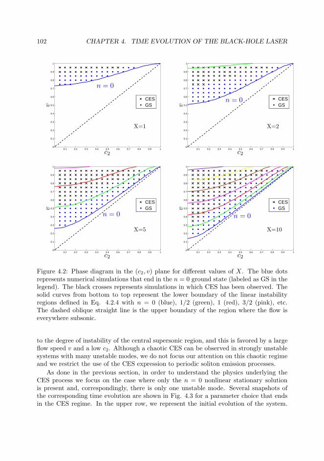
102 CHAPTER 4. TIME EVOLUTION OF THE BLACK-HOLE LASER
0.1 0.2 0.3 0.4 0.5 0.6 0.7 0.8 0.9 10
0.1
0.2
0.3
0.4
0.5
0.6
0.7
0.8
0.9
1
c2
v
X=1
CESGS
n = 0
0.1 0.2 0.3 0.4 0.5 0.6 0.7 0.8 0.9 10
0.1
0.2
0.3
0.4
0.5
0.6
0.7
0.8
0.9
1
c2
v
X=2
CESGS
n = 0
0.1 0.2 0.3 0.4 0.5 0.6 0.7 0.8 0.9 10
0.1
0.2
0.3
0.4
0.5
0.6
0.7
0.8
0.9
1
c2
v
X=5
CESGS
n = 0
0.1 0.2 0.3 0.4 0.5 0.6 0.7 0.8 0.9 10
0.1
0.2
0.3
0.4
0.5
0.6
0.7
0.8
0.9
1
c2
v
X=10
CESGS
n = 0
Figure 4.2: Phase diagram in the (c2, v) plane for different values of X . The blue dotsrepresents numerical simulations that end in the n = 0 ground state (labeled as GS in thelegend). The black crosses represents simulations in which CES has been observed. Thesolid curves from bottom to top represent the lower boundary of the linear instabilityregions defined in Eq. 4.2.4 with n = 0 (blue), 1/2 (green), 1 (red), 3/2 (pink), etc.The dashed oblique straight line is the upper boundary of the region where the flow iseverywhere subsonic.
to the degree of instability of the central supersonic region, and this is favored by a largeflow speed v and a low c2. Although a chaotic CES can be observed in strongly unstablesystems with many unstable modes, we do not focus our attention on this chaotic regimeand we restrict the use of the CES expression to periodic soliton emission processes.
As done in the previous section, in order to understand the physics underlying theCES process we focus on the case where only the n = 0 nonlinear stationary solutionis present and, correspondingly, there is only one unstable mode. Several snapshots ofthe corresponding time evolution are shown in Fig. 4.3 for a parameter choice that endsin the CES regime. In the upper row, we represent the initial evolution of the system.

4.3. NUMERICAL RESULTS 103
−50 −40 −30 −20 −10 0 10 20 30 40 500
0.2
0.4
0.6
0.8
1
1.2
1.4
1.6
1.8
2
x
ρ(x
)
t = 160
−50 −40 −30 −20 −10 0 10 20 30 40 500
0.2
0.4
0.6
0.8
1
1.2
1.4
1.6
1.8
2
x
ρ(x
)
t = 210
−50 −40 −30 −20 −10 0 10 20 30 40 500
0.2
0.4
0.6
0.8
1
1.2
1.4
1.6
1.8
2
x
ρ(x
)
t = 270
−50 −40 −30 −20 −10 0 10 20 30 40 500
0.2
0.4
0.6
0.8
1
1.2
1.4
1.6
1.8
2
x
ρ(x
)
t = 340
−20 −15 −10 −5 0 5 10 15 200
0.2
0.4
0.6
0.8
1
1.2
1.4
1.6
1.8
2
x
ρ(x
)
t = 1940
−20 −15 −10 −5 0 5 10 15 200
0.2
0.4
0.6
0.8
1
1.2
1.4
1.6
1.8
2
x
ρ(x
)
t = 1950
−20 −15 −10 −5 0 5 10 15 200
0.2
0.4
0.6
0.8
1
1.2
1.4
1.6
1.8
2
x
ρ(x
)
t = 1968
−20 −15 −10 −5 0 5 10 15 200
0.2
0.4
0.6
0.8
1
1.2
1.4
1.6
1.8
2
x
ρ(x
)
t = 1982
Figure 4.3: Snapshots of the condensate density (solid blue line) at different evolutiontimes (indicated in the panels) for a configuration with v = 0.95, c2 = 0.4 and X = 2 thateventually reaches the CES regime. The horizontal black line represent the initial ho-mogeneous condensate density. After some transient, the continuous emission of solitonsbegins. Upper row: initial evolution of the system when the initial linear instability setsin. The vertical black line marks the x = 0 position. Lower row: periodic evolution at latetimes after the system has reached the CES regime. The vertical dashed lines marks theboundaries of the supersonic region. At t = 1940, a soliton emerges near the black hole(subsonic-supersonic) interface at x < 0. This soliton cannot travel upstream and thenit bounces back, traveling to the downstream region and finally crossing the supersonicregion, see plot at t = 1950. After this soliton has left around t = 1968, the density growsagain and a new soliton starts growing near the interface. Finally, at t = 1982, the systemrecovers the same state as at t = 1940 and the process repeats.
We see that, after the onset of the initially instability, the emission of solitons begins.In the lower row, we analyze in detail the CES mechanism, which persists indefinitelyfor arbitrarily long times. The soliton that tries to be emitted in the upstream directionis dragged by the flowing condensate and bounces back. Eventually, it ends up in thedownstream region and travels towards x→ +∞. After the soliton has gone, the densitymodulation in the supersonic region begins to grow again until a new soliton is generated.Continuous periodic repetition of this process leads to the emission of a train of solitonsinto the downstream region.
In order to check quantitatively the periodicity of the soliton emission process, weintroduce the quantity tsol(N), which is defined as the time lapse between the emission ofthe consecutive (N − 1)th soliton and Nth soliton. If the emission of solitons is periodic,tsol should be constant and equal to the period. For counting solitons, we monitor thedensity at a generic point x0 ≫ X/2 in the downstream region as a function of time, asshown in the inset of Fig. 4.4. The minima of the density correspond to the passage ofa soliton. In the main panel we represent the time-evolution of the time lapse tsol(N).After some irregular transient, we see that this quantity approaches a constant value T ,

104 CHAPTER 4. TIME EVOLUTION OF THE BLACK-HOLE LASER
0 50 100 150 2000
100
200
300
400
500
600
700
Nsol
t sol
500 1000 1500 2000 2500 30000
0.2
0.4
0.6
0.8
1
1.2
1.4
1.6
1.8
2
t
ρ(x
0,t
)
Figure 4.4: Main panel: plot of tsol, the time lapse between the arrival of consecutivesolitons, as a function of the soliton number: after the emission of some solitons, thesystem reaches a regime of periodic soliton emission of period. Inset: time evolution ofthe density at a given point, ρ(x0, t) with x0 = 100. The density minima correspond tothe periodic passage of solitons. System parameters: v = 0.95, c2 = 0.4 and X = 2.
meaning that the soliton emission process becomes an almost perfectly periodic one.Interesting light on the soliton emission process can be obtained by studying the
dependence of the emission period on the system parameters. As an example, in Fig.4.5 we plot the CES period T as a function of c2 for fixed v = 0.95 and X = 2. Theplot stops at c2 = 0.77 since for larger values the CES dissapears and a sole soliton isemitted to the upstream region while the system relaxes to the n = 0 nonlinear solution,in the same line of Sec. 4.3.1. For c2 below the maximum value c2 = 0.77, the periodincreases with c2 as expected as for larger c2 the instability of the the supersonic regionbecomes weaker. The validity of this physical interpretation has been further confirmedby numerically checking that the period also increases when either v or X are decreased.
As a last ingredient before proposing a qualitative explanation of the CES mechanism,it is useful to remind a few crucial features of solitons in condensates (check Sec. (A fora detailed discussion on 1D GP solutions). As we have seen in the previous sections,solitons are often emitted into the upstream and/or downstream external regions in orderto compensate the increase of the density in the internal region. In the external region,the coupling constant is homogeneous g(x) = 1 and the condensate asymptotically flowsat a constant speed v. Hence, in the external regions, solitons are described by solutionsof the form
Ψ(x) = eivx[
ik +√
1− k2 tanh(√
1− k2 x)]
(4.3.4)
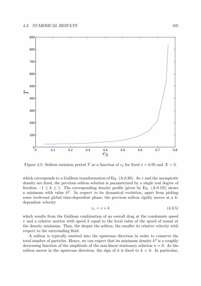
4.3. NUMERICAL RESULTS 105
0 0.1 0.2 0.3 0.4 0.5 0.6 0.7 0.80
100
200
300
400
500
600
700
800
900
c2
T
Figure 4.5: Soliton emission period T as a function of c2 for fixed v = 0.95 and X = 2.
which corresponds to a Galilean transformation of Eq. (A.0.20). As v and the asymptoticdensity are fixed, the previous soliton solution is parametrized by a single real degree offreedom −1 ≤ k ≤ 1. The corresponding density profile [given by Eq. (A.0.19)] showsa minimum with value k2. In respect to its dynamical evolution, apart from pickingsome irrelevant global time-dependent phase, the previous soliton rigidly moves at a k-dependent velocity
vs = v + k (4.3.5)
which results from the Galilean combination of an overall drag at the condensate speedv and a relative motion with speed k equal to the local value of the speed of sound atthe density minimum. Thus, the deeper the soliton, the smaller its relative velocity withrespect to the surrounding fluid.
A soliton is typically emitted into the upstream direction in order to conserve thetotal number of particles. Hence, we can expect that its minimum density k2 is a roughlydecreasing function of the amplitude of the non-linear stationary solution n = 0. As thesoliton moves in the upstream direction, the sign of k is fixed to k < 0. In particular,
106 CHAPTER 4. TIME EVOLUTION OF THE BLACK-HOLE LASER
we have numerically observed that the k parameter of the emitted soliton depends veryweakly on the initial condition so we can consider it to be a function of the systemparameters, k = k(v, c2, X). As the k parameter fixes the relative velocity of the solitonwith respect to the underlying fluid, a qualitative change of behavior is expected tooccur around v = |k(v, c2, X)|. For v < |k(v, c2, X)|, the soliton can freely travel in theupstream direction. In the opposite case, v > |k(v, c2, X)|, the flow speed v is larger thanthe relative soliton velocity |k|, so the soliton cannot travel to the upstream region andis dragged by the condensate flow into the downstream direction, originating the CESmechanism previously described.
Movies 7,8 and 9 illustrate this transition to the CES regime by reporting the result ofnumerical simulations for fixed v = 0.8, c2 = 0.4 and growing X = 2.2 (Movie 7), X = 2.4(Movie 8), and X = 2.5 (Movie 9). As X is increased, the soliton has to carry awaymore and more particles to allow the system to relax to the n = 0 nonlinear stationarystate, which implies a reduction of k. As a result, the soliton becomes slower and slower:while for X = 2.2 and X = 2.4 the soliton is able to escape to the upstream direction,compensating the higher density of the n = 0 nonlinear stationary solutions, this nolonger happens for X = 2.5, where we have in fact entered the v > k regime and thesoliton is forced to bounce back to the central region. As a result, it finally escapes in thedownstream direction leaving the system again in an unstable configuration, so that theCES process keeps periodically repeating for indefinite times.
Although this qualitative observation is in good agreement with the numerical results,it is far from offering a complete theoretical picture. In particular, finding a quantitativerelation between the minimum amplitude of the soliton emitted upstream and the param-eters of the system, i.e., the function k(v, c2, X), is still a theoretically unsettled problem.Obtaining and understanding this relation is an open question that should be addressedin future works.
The CES regime when several unstable modes are present can be much more complexdue to the appearance of other n > 0 nonlinear stationary solutions. Typically, the systememits several solitons before reaching the periodic CES regime described previously. Weshow this scenario in Movie 10, which summarizes the result of a simulation for v =0.65, c2 = 0.3, X = 8. In other situations, the system first evolves towards a n > 0solution, remains in the vicinity of such solution for quite some time, then departs againfrom it and, after some transient, reaches the CES regime. We show an example ofthis latter case in Movie 11. In this simulation, the system stays in the vicinity of thedynamically unstable n = 1 solution for quite some time before entering in the CESregime. Finally, for a large number of unstable modes, the periodicity of the solitonemission may completely disappear, with the system strongly oscillating around differentsolutions with n > 0. This chaotic scenario is illustrated in Movie 12, where the systemshows a very complicated aperiodic emission of solitons.
4.4 Discussion and comparison with optical lasers
On the basis of the results presented in the previous Sections, we are now in a positionto critically discuss the actual physical content of the widely used expression black-hole
4.4. DISCUSSION AND COMPARISON WITH OPTICAL LASERS 107
laser.Historically, when this expression was first introduced by Corley and Jacobson [83],
the authors had in mind the linear dynamical instability of the configuration with a pair ofneighbouring black- and white-hole horizons. In terms of laser devices in quantum optics,this dynamical instability corresponds to the linear instability of the electromagneticvacuum state of the cavity when the (unsaturated) gain exceeds losses. In this case,any weak signal due to, e.g., spontaneous emission, is able to trigger the instability andquickly gets coherently amplified by stimulated emission.
The actual operation of a continuous-wave laser device [87, 33, 88, 89] takes place ina very different regime, where nonlinear gain saturation brings the system to a nonlinearstationary state where (saturated) gain and losses exactly compensate each other and thefield keeps oscillating at a well-defined frequency with a well-defined amplitude. This cleanand coherent laser emission is attained at long times after switch-on once all (possiblycomplex) transient phenomena are gone: from the point of view of the field dynamics, thelong-time limit is a limit cycle in the classical dynamics, and the only observable quantumeffect are small fluctuations in the oscillation frequency, leading to a very long but finitecoherence time of the emission.
Even though from a quantum optics perspective the expression black-hole laser sug-gests a spontaneously oscillating behavior with no memory of the initial state and stronglydetermined by nonlinear effects, the complex nonlinear dynamics of analog models inthe two-horizon configurations has began being investigated only very recently in Refs.[85, 86]. Building on top of these works, we have seen in the previous sections that thelong-time behavior of such configurations is much richer than that of standard opticallasers.
In many cases (Sec. 4.3.1), the system is in fact able to quickly find a new time-independent stationary state where the instability is suppressed by a suitable redistri-bution of the density which eliminates the supersonic character of the central region.During this rapid “evaporation” of the horizons, the extra energy and particle densityare compensated by the emission of a short sequence of sound and solitons to the outerregions.
On the other hand, regimes (Sec. 4.3.2) where the density keeps oscillating in aperiodic way in time can be regarded as a hydrodynamic counterpart of a continuous-wavemonochromatic optical laser oscillation, leading to a continuous and periodic emission oftrains of solitons. The excellent periodicity and insensitivity to initial conditions of thissoliton train guarantees a very high degree of coherence of the emission, closely analogousto that of the output beam of an optical laser device. On this basis, a rigorous readermay then argue that the black-hole lasing expression should only be used to refer to thislatter case.
As a final remark, it is worth noting that in contrast to standard single-mode laserdevices which emit light of a single frequency, the solitons emitted by the BH laser deviceare intrinsically nonlinear objects containing a number of frequency components. Dif-ferently from pulsed lasers where the pulse-generating mechanism serves to modulate amuch faster carrier frequency and creates tightly spaced sidebands, here the nonlinearityprovides new frequencies at integer multiples of the fundamental one. In a qualitativepicture, these components can be understood as resulting from a phase-locking of the
108 CHAPTER 4. TIME EVOLUTION OF THE BLACK-HOLE LASER
different modes of the central, super-sonic region that are simultaneously oscillating. Theenergy for these oscillations is provided by the macroscopic flow of the condensate, andthe mechanism responsible for the phase-locking of the different components originatesfrom the hydrodynamic nonlinearities at large density modulations.
4.5 Conclusions and outlook
In this chapter, we have presented an extensive campaign of numerical simulations ofthe GP equation describing the time-evolution of a Bose-Einstein condensate in a BHlaser scenario. In agreement with existing theoretical results about linear instabilitiesand nonlinear stationary solutions, our simulations provide useful physical insight on thesystem behavior as a function of the initial system parameters. In some cases, the centralsupersonic region is eventually evaporated away and the system at late times approachesa stationary stable configuration; in other cases, the system approaches a novel regime ofcontinuous and periodic emission of solitons (CES) for indefinite times.
For different reasons, both regimes have a potentially strong interdisciplinary interest.On the one hand, the horizon evaporation process studied in our numerical simulationsis a classical counterpart of black-hole evaporation under the effect of the spontaneousHawking emission. From this point of view, a full understanding of the classical dynamicsof the black-hole laser under the back-reaction effect of the classical emission is a naturalfirst step towards a quantitative modeling of the back-reaction of quantum fluctuationson the curved space-time metric of an astrophysical black hole [95].
On the other hand, interesting analogies and differences between the continuous soli-ton emission in black-hole lasers and the operation of an optical laser device can be drawnfrom our simulations. On this basis, a more restrictive use of the black-hole laser expres-sion is proposed. While all our discussion has focussed on the classical black-hole laserdynamics, future work will address the effect of quantum fluctuations on these systems:taking again inspiration from quantum optics and laser theory, we may legitimately ex-pect that quantum effects should reduce to weak fluctuations in the emission frequencyand, therefore, to a slow decoherence of the soliton emission analogous to the long, butfinite coherence time of optical laser devices [87, 33, 88, 89]. A more deep understandingof the CES regime should be also provided by forthcoming theoretical works.
Apart from the gravitational considerations, the CES regime here described can alsorepresent an interesting scenario for the fields of quantum transport and atomtronics sinceit provides the soliton analog of an optical laser in a Bose-Einstein condensate.
From the experimental point of view, we can reasonably expect that an upgraded ver-sion of the ultracold atom experiment in [21] will soon be able to investigate the nonlineardynamics of the black-hole laser at late times after the onset of the dynamical instabilityand hopefully characterize the rich phenomenology discussed in this work. Even thoughall the discussion in this work has been carried out having an atomic implementationin mind, we expect that most conclusions can be directly transferred to analog modelsbased on fluids of light in the so-called propagating geometry, for which theoretical workson black hole configurations have recently appeared [96, 97] as well as first experimentalevidences of superfluid behaviors [98].
Part II
Thermal clouds
109

Chapter 5Thermal decay in a trapped gas
5.1 Introduction
In the first part of this thesis, we have studied the implementation of gravitational ana-logues in condensed-matter systems. In particular, we have focused on Bose gases nearT = 0, where the mean-field Gross-Pitaevskii equation is valid. In this chapter, we switchto the opposite limit: a gas of bosons above the critical temperature Tc. In particular,we analyze the response of a thermal cloud (without any condensed fraction) to the ap-plication of a short Bragg pulse. As one may expect, this process induces oscillations inthe density profile that eventually decay after removing the lattice potential. Followingthe standard textbooks on the field [26, 27], one would typically attribute the dampingmechanism to the collisional relaxation of the collective modes above Tc, described usingthe classical Boltzmann distribution function. However, we show in this chapter thatthe decay of the oscillations is actually due to the thermal disorder of the particles andshows a characteristic time scale that only depends on the temperature T , the mass of theatoms m and the wave vector of the Bragg lattice k. This result is found when using bothquantum and classical formalisms. Indeed, we show that this thermal decay is a generalfeature of the introduction of an arbitrary spatially periodic pulse. Moreover, under somegeneral assumptions, the results here presented can be applied to other systems such agas of bosons below Tc (with some condensed fraction present) or a gas of fermions athigh temperatures.
We start the chapter by describing the physical setup in Sec. 5.2. After that, undercertain specific assumptions, we provide a theoretical explanation for the phenomenon,using both classical (Sec. 5.3) and quantum (Sec. 5.4) formalisms. We discuss the validityand physical meaning of the approximations used and unify the quantum and classicalresults in Sec. 5.5. The obtained results are generalized to broader scenarios in Sec. 5.6.We finally compare the results from the calculations with actual experimental data inSec. 5.7. The conclusions are drawn in Sec. 5.8.
111
112 CHAPTER 5. THERMAL DECAY IN A TRAPPED GAS
5.2 Physical setup
We consider an initially confined cloud of N bosonic atoms at thermal equilibrium withtemperature T > Tc, so there is no condensate. The atomic cloud is confined by theharmonic trap created by the potential
Vtrap(x) =∑
i
1
2mw2
i x2i (5.2.1)
with i = 1, 2, 3 labeling the coordinates x, y, z. Then, at t = 0, a short Bragg pulse isswitched on during a time τ , inducing a sinusoidal potential in the z direction of the form
V (z, t) = −χ(
t
τ
)
V0 cos(kz) (5.2.2)
where χ is the characteristic function of the interval [0, 1].This Bragg pulse is created by two incident laser beams with same wavelength and
forming some angle between them, in the same way as the optical lattice considered inChapter 2. After time τ , the pulse is switched off and the atom cloud is left to evolvewithin the trap. As we will show in this work, the Fourier components of the formeddensity pattern decay with a Gaussian behavior and the density returns to the initialequilibrium configuration. The introduction of a short Bragg pulse was also appliedbelow Tc for measuring the phonon dispersion relation [99].
For studying the dynamics of the previous scenario, we consider both quantum andclassical descriptions. In the two models we neglect interaction between particles, see Sec.5.5.2 for a detailed discussion on the role of interactions.
5.3 Classical description
As a first step, we study the problem in a classical context. For that purpose, we usethe Boltzmann equation, which governs the time evolution of the Boltzmann distributionfunction f(x,p, t) that gives the density in both real and momentum space [26, 27]. TheBoltzmann equation, for non-interacting particles, can be written as:
∂f
∂t+
p
m∇f + Fext∇pf = 0 (5.3.1)
where ∇p denotes the gradient with respect the momentum components and Fext is theforce that acts on the particles due to the external field, Fext = −∇H , with H the totalHamiltonian. The general solution of Eq. (5.3.1) can be computed using the method ofcharacteristics:
f(x,p, t) = f0(x0(x,p, t),p0(x,p, t)) (5.3.2)
where f0(x,p) is the initial Boltzmann distribution function at t = 0. The vectorsx0(x,p, t), p0(x,p, t) are initial conditions at t = 0 such their time evolution through theclassical equations of motion will carry them to x,p in a time t or, from another pointof view, they are the result of integrating the corresponding time-reversed equations of
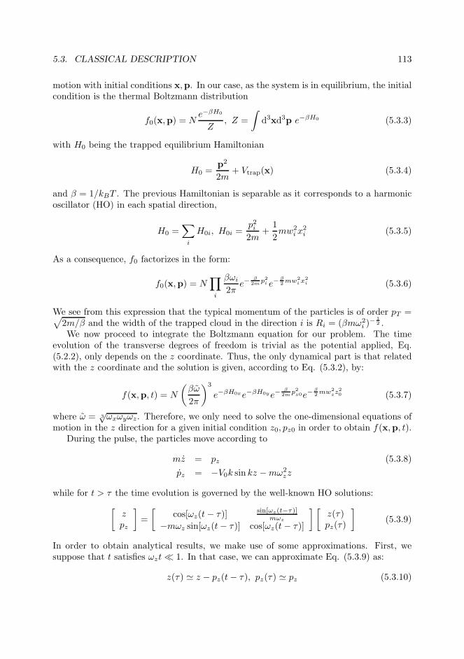
5.3. CLASSICAL DESCRIPTION 113
motion with initial conditions x,p. In our case, as the system is in equilibrium, the initialcondition is the thermal Boltzmann distribution
f0(x,p) = Ne−βH0
Z, Z =
∫
d3xd3p e−βH0 (5.3.3)
with H0 being the trapped equilibrium Hamiltonian
H0 =p2
2m+ Vtrap(x) (5.3.4)
and β = 1/kBT . The previous Hamiltonian is separable as it corresponds to a harmonicoscillator (HO) in each spatial direction,
H0 =∑
i
H0i, H0i =p2i2m
+1
2mw2
i x2i (5.3.5)
As a consequence, f0 factorizes in the form:
f0(x,p) = N∏
i
βωi
2πe−
β2mp2
i e−β2 mw2
i x2i (5.3.6)
We see from this expression that the typical momentum of the particles is of order pT =√
2m/β and the width of the trapped cloud in the direction i is Ri = (βmω2i )
− 12 .
We now proceed to integrate the Boltzmann equation for our problem. The timeevolution of the transverse degrees of freedom is trivial as the potential applied, Eq.(5.2.2), only depends on the z coordinate. Thus, the only dynamical part is that relatedwith the z coordinate and the solution is given, according to Eq. (5.3.2), by:
f(x,p, t) = N
(
βω
2π
)3
e−βH0xe−βH0ye−β
2mp2z0e−
β2 mw2
zz20 (5.3.7)
where ω = 3√ωxωyωz. Therefore, we only need to solve the one-dimensional equations of
motion in the z direction for a given initial condition z0, pz0 in order to obtain f(x,p, t).During the pulse, the particles move according to
mz = pz (5.3.8)
pz = −V0k sin kz −mω2zz
while for t > τ the time evolution is governed by the well-known HO solutions:
[
zpz
]
=
[
cos[ωz(t− τ)] sin[ωz(t−τ)]mωz
−mωz sin[ωz(t− τ)] cos[ωz(t− τ)]
] [
z(τ)pz(τ)
]
(5.3.9)
In order to obtain analytical results, we make use of some approximations. First, wesuppose that t satisfies ωzt≪ 1. In that case, we can approximate Eq. (5.3.9) as:
z(τ) ≃ z − pz(t− τ), pz(τ) ≃ pz (5.3.10)

114 CHAPTER 5. THERMAL DECAY IN A TRAPPED GAS
In the previous approximation, we have neglected the variation of momentum resultingfrom the term mωzz sin[ωz(t − τ)] as it represents a small correction to the thermalmomentum of the particles, mωzz sin[ωz(t− τ)] ∼ mωzRzωz(t− τ) ∼ pTωz(t− τ) ≪ pT .The same argument can be applied to the harmonic oscillator part of Eq. (5.3.8) and thenit is reduced to pz ≃ −V0k sin kz. This equation can be integrated in terms of ellipticfunctions, as it corresponds to a classical pendulum. In this way, we express z0 in termsof z(τ) as:
z0 =2
karcsin
(
ν sn
[
F
(
arcsin
(
kz(τ)2
ν
)
, ν
)
−√
V0mkτ, ν
])
, ν =E + V02V0
, E < V0
z0 =2
karcsin sn
[
F
(
kz(τ)
2, ν
)
−√
E + V02m
kτ, ν
]
, ν =2V0
E + V0, E > V0 (5.3.11)
with E the conserved energy during the presence of the Bragg pulse:
E =p2z(τ)
2m− U cos [kz(τ)] =
p2z02m
− U cos [kz0] (5.3.12)
from which we can also obtain the momentum pz0. For the notation of elliptic functions,see Eq. (A.0.13) and associated discussion.
If the increase in the momentum due to the force of the pulse satisfy V0kτ/pT . 1,then pT is still the typical momentum of the particles after the pulse. This implies that,as the total displacement of the z coordinate is of order z ∼ z0 + vT t, with vT = pT /mthe thermal velocity of the atoms, βmω2
zz20 ≃ βmω2
zz2 with corrections O(ωzt). Hence,
we set z0 = z in Eq. (5.3.7):
f(x,p, t) ≃ N
(
βω
2π
)3
e−βVtrap(x)e−β
2mp2xe−
β2mp2
ye−β
2mp2z0 (5.3.13)
We see that the previous approximations amount to consider the gas as locally homo-geneous, with an envelope factor e−βVtrap(x), similar to the local density approximationthat we will consider in Sec. 5.4.2. The only remaining task is to compute pz0. Althoughit can be expressed in terms of elliptic functions from the results of Eq. (5.3.11), in orderto obtain explicit formulas for the density we assume that the pulse duration τ is suffi-ciently small for a Runge-Kutta second-order approximation to be valid. In that case, wecompute the time evolution during the pulse as:
pz0 ≃ pz + V0kτ sin kz(τ
2
)
, z(τ
2
)
≃ z(τ)− pzτ
2m= z − pz
mt (5.3.14)
with t ≡ t − τ/2 and we have used that pz = pz(τ), following Eq. (5.3.10). The firstcorrections to the previous equation are O(τ3). We refer to Sec. 5.5.3 for a detailedanalysis of the validity of the previous approximation.
The density is obtained after integrating over the momentum variables of f(x,p, t) inEq. (5.3.13):
n(x, t) =
∫
d3p f(x,p, t) = N
(
βmω2
2π
)32
e−βVtrap(x)G(z, t) (5.3.15)
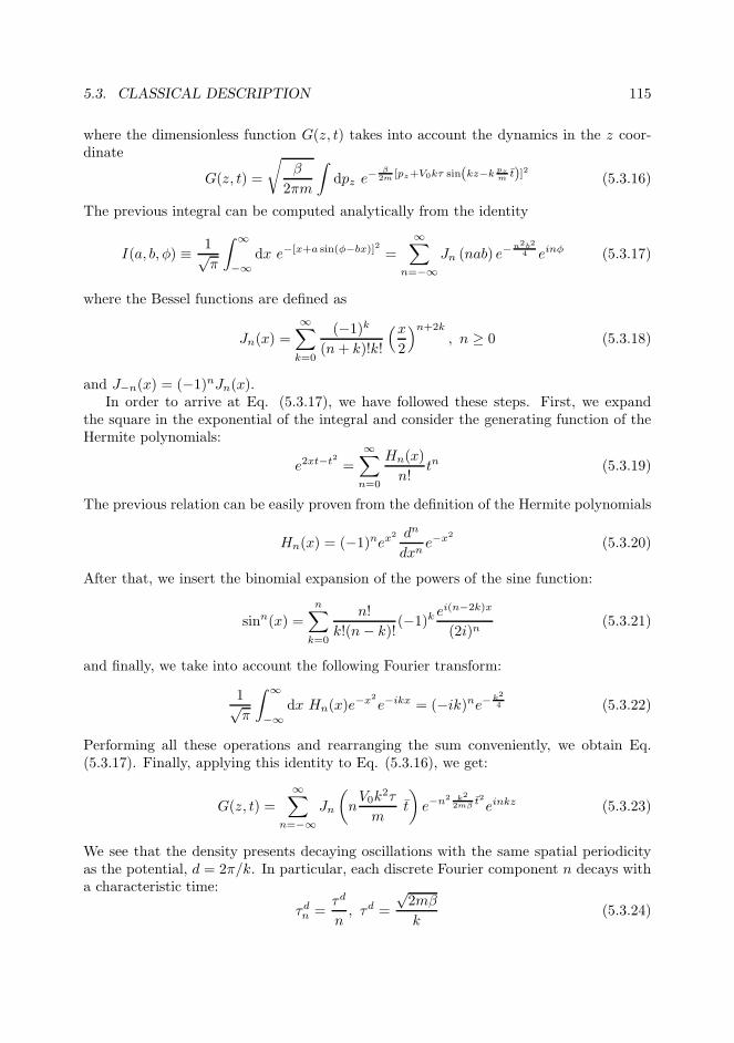
5.3. CLASSICAL DESCRIPTION 115
where the dimensionless function G(z, t) takes into account the dynamics in the z coor-dinate
G(z, t) =
√
β
2πm
∫
dpz e− β
2m [pz+V0kτ sin(kz−k pzm
t)]2 (5.3.16)
The previous integral can be computed analytically from the identity
I(a, b, φ) ≡ 1√π
∫ ∞
−∞dx e−[x+a sin(φ−bx)]2 =
∞∑
n=−∞Jn (nab) e
−n2b2
4 einφ (5.3.17)
where the Bessel functions are defined as
Jn(x) =∞∑
k=0
(−1)k
(n+ k)!k!
(x
2
)n+2k
, n ≥ 0 (5.3.18)
and J−n(x) = (−1)nJn(x).In order to arrive at Eq. (5.3.17), we have followed these steps. First, we expand
the square in the exponential of the integral and consider the generating function of theHermite polynomials:
e2xt−t2 =
∞∑
n=0
Hn(x)
n!tn (5.3.19)
The previous relation can be easily proven from the definition of the Hermite polynomials
Hn(x) = (−1)nex2 dn
dxne−x2
(5.3.20)
After that, we insert the binomial expansion of the powers of the sine function:
sinn(x) =n∑
k=0
n!
k!(n− k)!(−1)k
ei(n−2k)x
(2i)n(5.3.21)
and finally, we take into account the following Fourier transform:
1√π
∫ ∞
−∞dx Hn(x)e
−x2
e−ikx = (−ik)ne−k2
4 (5.3.22)
Performing all these operations and rearranging the sum conveniently, we obtain Eq.(5.3.17). Finally, applying this identity to Eq. (5.3.16), we get:
G(z, t) =
∞∑
n=−∞Jn
(
nV0k
2τ
mt
)
e−n2 k2
2mβt2einkz (5.3.23)
We see that the density presents decaying oscillations with the same spatial periodicityas the potential, d = 2π/k. In particular, each discrete Fourier component n decays witha characteristic time:
τdn =τd
n, τd =
√2mβ
k(5.3.24)
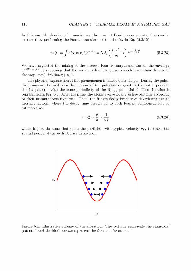
116 CHAPTER 5. THERMAL DECAY IN A TRAPPED GAS
In this way, the dominant harmonics are the n = ±1 Fourier components, that can beextracted by performing the Fourier transform of the density in Eq. (5.3.15):
nk(t) =
∫
d3x n(x, t)e−ikz = NJ1
(
V0k2τ
mt
)
e−(t
τd )2
(5.3.25)
We have neglected the mixing of the discrete Fourier components due to the envelopee−βVtrap(x) by supposing that the wavelength of the pulse is much lower than the size ofthe trap, exp(−k2/βmω2
z) ≪ 1.
The physical explanation of this phenomenon is indeed quite simple. During the pulse,the atoms are focused onto the minima of the potential originating the initial periodicdensity pattern, with the same periodicity of the Bragg potential d. This situation isrepresented in Fig. 5.1. After the pulse, the atoms evolve locally as free particles accordingto their instantaneous momenta. Then, the fringes decay because of disordering due tothermal motion, where the decay time associated to each Fourier component can beestimated as
vT τdn ∼ d
n∼ 1
nk(5.3.26)
which is just the time that takes the particles, with typical velocity vT , to travel thespatial period of the n-th Fourier harmonic.
x
V
Figure 5.1: Illustrative scheme of the situation. The red line represents the sinusoidalpotential and the black arrows represent the force on the atoms.

5.4. QUANTUM DESCRIPTION 117
5.4 Quantum description
We now consider a quantum description, using the second-quantization formalism tocompute all the desired magnitudes. We first present a general review of the initialequilibrium configuration, where many of the results can be consulted in the standardliterature of the field [26, 27]. After that, following the techniques developed for theequilibrium study, we compute the dynamical evolution of the density. Throughout thischapter, when dealing with second-quantization operators, we write them with “hats” inorder to distinguish them from their first-quantization equivalents.
5.4.1 Equilibrium properties
In equilibrium, the system is described by the density matrix
ρ =e−βK
Q, Q = Tr
(
e−βK)
(5.4.1)
where K = H0 − µN is the grand-canonical Hamiltonian and the operator H0 is thesecond-quantized version of the trap Hamiltonian (5.3.4). The equilibrium density can becomputed from:
n0(x) = 〈Ψ†(x)Ψ(x)〉 = Tr(
Ψ†(x, t)Ψ(x, t)ρ)
(5.4.2)
where the stationary field operator is given by:
Ψ(x) =∑
n
Ψn(x)an (5.4.3)
Ψn(x) being the single-particle eigenfunctions of the (first-quantized) equilibrium Hamil-tonian H0, with eigenenergy εn, and an their associated second-quantized annihilationoperators. Here, n labels any possible quantum number of the eigenfunctions.
From the previous results, it is straightforward to prove that the density is given by:
n0(x) =∑
n
|Ψn(x)|21
eβ(εn−µ) − 1(5.4.4)
which simply shows that the total density is just the sum of the Bose-Einstein occupationnumber of every state multiplied by its associated spatial probability density. Integratingover all the space, the total number of particles is:
N =
∫
d3x n0(x) =∑
n
1
eβ(εn−µ) − 1(5.4.5)
These are the usual results found in the textbooks for a Bose gas. However, for furthercalculations, it is useful to rewrite the previous identities in a more convenient way. Takinginto account the identity
x
1− x= x
∞∑
j=0
xj =
∞∑
j=1
xj (5.4.6)
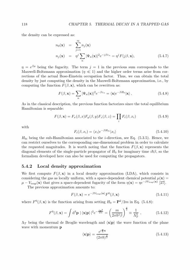
118 CHAPTER 5. THERMAL DECAY IN A TRAPPED GAS
the density can be expressed as:
n0(x) =
∞∑
j=1
nj(x)
nj(x) = ηj∑
n
|Ψn(x)|2e−jβεn = ηjF (jβ,x), (5.4.7)
η = eβµ being the fugacity. The term j = 1 in the previous sum corresponds to theMaxwell-Boltzmann approximation (η ≪ 1) and the higher order terms arise from cor-rections of the actual Bose-Einstein occupation factor. Thus, we can obtain the totaldensity by just computing the density in the Maxwell-Boltzmann approximation, i.e., bycomputing the function F (β,x), which can be rewritten as:
F (β,x) =∑
n
|Ψn(x)|2e−βεn = 〈x|e−βH0 |x〉 , (5.4.8)
As in the classical description, the previous function factorizes since the total equilibriumHamiltonian is separable:
F (β,x) = Fx(β, x)Fy(β, y)Fz(β, z) =∏
i
Fi(β, xi) (5.4.9)
withFi(β, xi) = 〈xi|e−βH0i |xi〉 (5.4.10)
H0i being the sub-Hamiltonian associated to the i-direction, see Eq. (5.3.5). Hence, wecan restrict ourselves to the corresponding one-dimensional problem in order to calculatethe requested magnitudes. It is worth noting that the function F (β,x) represents thediagonal elements of the single-particle propagator of H0 for imaginary time i~β, so theformalism developed here can also be used for computing the propagators.
5.4.2 Local density approximation
We first compute F (β,x) in a local density approximation (LDA), which consists inconsidering the gas as locally uniform, with a space-dependent chemical potential µ(x) =µ− Vtrap(x) that gives a space-dependent fugacity of the form η(x) = ηe−βVtrap(x) [27].
The previous approximation amounts to:
F (β,x) = e−βVtrap(x)F 0(β,x) (5.4.11)
where F 0(β,x) is the function arising from setting H0 = P2/2m in Eq. (5.4.8):
F 0(β,x) =
∫
d3p | 〈x|p〉 |2e− βp2
2m =
(
m
2π~2β
)32
≡ 1
Λ3T
, (5.4.12)
ΛT being the thermal de Broglie wavelength and 〈x|p〉 the wave function of the planewave with momentum p
〈x|p〉 = eip~x
(2π~)32
(5.4.13)
5.4. QUANTUM DESCRIPTION 119
Then, in the LDA,
F (β,x) =e−βVtrap(x)
Λ3T
(5.4.14)
and the total density reads
n0(x) =g 3
2[η(x)]
Λ3T
, gs(z) ≡∞∑
j=1
zj
js(5.4.15)
which is the usual relation for a homogeneous ideal gas but replacing η by its space-dependent version η(x), as previously explained. Integrating, we find:
N =g3(η)
(β~ω)3(5.4.16)
which allows us to write
n0(x) = N
(
βmω2
2π
)32 g 3
2[η(x)]
g3(η)(5.4.17)
that gives the classical expression for η ≪ 1. In the opposite limit, a phase transition toa Bose-Einstein condensate occurs at T such that η = 1. As gs(1) = ζ(s), with ζ(s) theRiemann zeta function, we find that the ideal critical temperature T 0
c is given by:
kBT0c =
(
N
ζ(3)
)13
~ω (5.4.18)
As explained later, the LDA corresponds to the ideal thermodynamic limit of aninfinite number of particles.
5.4.3 Harmonic oscillator
On the other hand, we note that for a HO-type Hamiltonian the previous magnitudescan be also computed analytically. Since the full Hamiltonian H0 is separable, we have acollection of 1D HOs so we first review the general properties of the 1D HO Hamiltonian:
H =P 2
2m+
1
2mω2X2 = ~ω
(
a†a+1
2
)
a =Xl + iP
~l√
2, l =
√
~
mω(5.4.19)
In the previous expression, X,P are the position and momentum operators and l theharmonic oscillator length. The annihilation operator a satisfies the well-known commu-tation relation [a, a†] = 1. The eigenvalues and eigenstates of the HO Hamiltonian arethe well-known number states:
H |n〉 = ~ω
(
n+1
2
)
|n〉 , |n〉 = (a†)n√n!
|0〉 , n = 0, 1, 2 . . . (5.4.20)
〈x|n〉 ≡ 1√
2nn!√πlHn(
x
l)e−
x2
2l2

120 CHAPTER 5. THERMAL DECAY IN A TRAPPED GAS
We also introduce the coherent states |α〉, where α is a complex number, as they willbe very useful for our calculations. They are the eigenstates of the annihilation operatora |α〉 = α |α〉,
|α〉 = e−|α|22
∞∑
n=0
αn
√n!
|n〉 = eαa†−α∗a |0〉 (5.4.21)
where the rightmost relation follows from Eq. (5.5.6). It is straightforward to show fromthis expression that, for any complex number z,
eza†a |α〉 = e−
(1−|e2z |)|α|22 |ezα〉 (5.4.22)
The spatial representation of the coherent states reads
〈x|α〉 =e−
(x−√
2α1l)2
2l2
π14 l
12
ei√2α2
xl e−iα1α2 =
e−x2
2l2
π14 l
12
e√2α x
l e−α21e−iα1α2
=e−
x2
2l2
π14 l
12
e√2α x
l e−|α|22 e−
α2
2 (5.4.23)
where α1,2 are the real and imaginary parts of α, α = α1 + iα2. The previous identitycan be obtained by expanding a in terms of the position and momentum operators X,Pin Eq. (5.4.21) or well by using the generating function of Eq. (5.3.19) and the spatialrepresentation of |n〉. It can also be proven, from Eq. (5.4.21), that the coherent statesform an overcomplete set of states of the Hilbert state:
1 =1
π
∫
d2α |α〉 〈α| , d2α = dα1dα2 (5.4.24)
Another useful identity follows from Eq. (5.4.23)
eγxl 〈x|α〉 = e
γ2
4 e|γ|24 e
(α+α∗)γ+(γ+γ∗)α
2√
2 〈x|α + iγ√2〉 , (5.4.25)
satisfied for any complex number γ.
The above results allow us to rewrite in a more convenient way the operator e−βH :
e−βH = e−βH 1
π
∫
d2α |α〉 〈α| = e−β~ω2
π
∫
d2α e−(1−e−2β~ω )|α|2
2 |e−β~ωα〉 〈α|
=e
β~ω2
π
∫
d2α e− sinh(β~ω)|α|2 |e− β~ω2 α〉 〈e β~ω
2 α| (5.4.26)
We are now in a position to compute the equilibrium density since it is expressed in terms
5.4. QUANTUM DESCRIPTION 121
of the spatial diagonal matrix elements of e−βH :
〈x|e−βH |x〉 =e
β~ω2 e−
x2
l2
lπ32
∫
d2α e−12α
TMα+vT α (5.4.27)
M =
[
4 cosh(β~ω) + 2 sinh(β~ω) −2i sinh(β~ω)−2i sinh(β~ω) 2 sinh(β~ω)
]
α =
[
α1
α2
]
v =√2x
l
(
e−β~ω2
[
1i
]
+ eβ~ω2
[
1−i
])
We have introduced some vectorial magnitudes in order to simplify the notation. Notethat the matrix M is a symmetric complex matrix. If we write M = A + iB, withA,B real symmetric matrices, the previous integral only converges for A > 0. In thatcase, M can be reduced to a diagonal matrix by the transformation UTMU = D, with
U = OD−1/2A OD
1/2A , being O the orthogonal matrix that diagonalizes A, DA = OTAO,
and O the orthogonal matrix that diagonalizes D−1/2A OTBOD
−1/2A . As U is a real matrix
and | detU | = 1, we arrive at the usual result for Gaussian integrals for definite positivereal matrices:
∫
d2α e−12α
T Mα+vTα =2π√detM
e12v
TM−1v (5.4.28)
The previous formula trivially generalizes to n dimensions by replacing 2π by (2π)n/2.Applying this result to Eq. (5.4.27), we find:
〈x|e−βH |x〉 =√
mω
2π~ sinh(β~ω)e− tanh(β~ω
2 )mω~
x2
(5.4.29)
Turning back to our physical problem, the last equation gives directly the values ofFi in Eq. (5.4.10) by just changing ω by ωi:
Fi(β, xi) =
√
mωi
2π~ sinh(β~ωi)e− tanh
(
β~ωi2
)
mωi~
x2i (5.4.30)
From here, after integrating and performing some straightforward manipulations, thetotal number of particles can be expressed as:
N =
∞∑
j=1
ηj
8 sinh(
j β~ωx
2
)
sinh(
jβ~ωy
2
)
sinh(
j β~ωz
2
) (5.4.31)
We note that, for the full HO Hamiltonian, the phase transition occurs when the chemicalpotential is equal to the zero-point energy
µ = ε0 =3~ωm
2, ωm =
ωx + ωy + ωz
3, (5.4.32)

122 CHAPTER 5. THERMAL DECAY IN A TRAPPED GAS
ωm being the mean frequency. Absorbing the zero-point energy in the definition of thechemical potential, η ≡ ηe−βε0 , the previous condition is equivalent to η = 1. After thisredefinition, the expression for the total number of particles reads:
N =
∞∑
j=1
ηjejβε0
8 sinh(
j β~ωx
2
)
sinh(
jβ~ωy
2
)
sinh(
j β~ωz
2
) (5.4.33)
In the limit β~ωm ≪ 1 (which implies β~ωi ≪ 1) we recover the result of Eq. (5.4.16).Moreover, we can also compute the first correction to the LDA, given by:
N =g3(η)
(β~ω)3+
3
2
ωm
ω
g2(η)
(β~ω)2(5.4.34)
This correction shifts the critical temperature by an amount δTc ≡ Tc − T 0c , with T
0c the
ideal critical temperature obtained in the LDA, which is perturbatively obtained fromthe previous equation:
δTcT 0c
= −βc~ωmζ(2)
2ζ(3)= −ωm
2ω
ζ(2)
ζ23 (3)
N− 13 ≈ −0.73
ωm
ωN− 1
3 (5.4.35)
The rightmost expression tells us that the corrections to the LDA arise from the actualfinite number of particles. For sufficiently large number of particles N , however, thesecorrections are negligible. Therefore, the LDA corresponds to the thermodynamic limitN → ∞. On the other hand, the previous relation implies that, if finite-size effects aresmall, βc~ωm ≪ 1 and then, as we are dealing with temperatures T & Tc, β~ωm ≪ 1.Thus, the LDA is valid whenever the previous finite-size correction is small. We discussin more detail these conditions in Sec. 5.5.1.
Interestingly, the previous results can also be obtained directly from the sum of theseries of Eq. (5.4.5)
N =∑
n
1
eβ(εn−µ) − 1, εn = ε0 +
∑
i
ni~ωi (5.4.36)
where n = (nx, ny, nz) are the quantum numbers of the oscillators in each direction.After absorbing the zero-point energy in the chemical potential, expanding the previousexpression using Eq. (5.4.6) and performing first the summations over the ni quantumnumbers, which are just the usual harmonic series, we arrive at Eq. (5.4.31).
5.4.4 Dynamical evolution
After reviewing the thermodynamic properties of the initial state of the trapped cloud,we return to our dynamical problem. Similar to Eq. (5.4.2), the time-dependent densityreads:
n(x, t) = 〈Ψ†(x, t)Ψ(x, t)〉 = Tr(
Ψ†(x, t)Ψ(x, t)ρ)
(5.4.37)

5.4. QUANTUM DESCRIPTION 123
where Ψ(x, t) is now the time evolution of the field operator Ψ(x) of Eq. (5.4.3) inthe Heisenberg picture while ρ is the same equilibrium state of Eq. (5.4.1). As we areneglecting interactions, the time-evolution of the field operator is:
Ψ(x, t) =∑
n
Ψn(x, t)an (5.4.38)
with Ψn(x, t) the time-evolution of the eigenfunction Ψn(x) under the total first-quantizationHamiltonian
H = H0 + V (z, t) (5.4.39)
with V (z, t) being the potential of the perturbation of Eq. (5.2.2). Following the samereasonings leading to Eq. (5.4.7), we can write the expression for the density as
n(x, t) =
∞∑
j=1
nj(x, t)
nj(x, t) = ηjF (jβ,x, t), (5.4.40)
and F (β,x, t) is now
F (β,x, t) =∑
n
|Ψn(x, t)|2e−βεn = 〈x|U(t)e−βH0U †(t)|x〉 , (5.4.41)
with U(t) being the time-evolution operator associated to the Hamiltonian (5.4.39). Fol-lowing the same reasoning as in the classical calculation, only the z-coordinate has anon-trivial time evolution and then the function F (β,x, t) factorizes in the form:
F (β,x, t) = Fx(β, x)Fy(β, y)Fz(β, z, t) (5.4.42)
where the functions associated to the transverse coordinates are those of the equilibriumstate and the dynamical part is:
Fz(β, z, t) = 〈z|Uz(t)e−βH0zU †
z (t)|z〉 (5.4.43)
with Uz(t) the time evolution operator in the longitudinal direction. For times t > τ ,Uz(t) is given by:
Uz(t) = e−iH0z~
(t−τ)Uτ (5.4.44)
Uτ = e−iH0z~
τ+iu cos(kz) (5.4.45)
u ≡ V0τ
~(5.4.46)
For the computation of the function F (β,x, t), in the same fashion as in the equilibriumstate, we first consider the local density approximation and after that we perform thecomplete calculation using the full Hamiltonian.
124 CHAPTER 5. THERMAL DECAY IN A TRAPPED GAS
Local density approximation
As previously explained, the LDA consists in considering the gas as locally homogeneouswith an space-dependent chemical potential. Following the same reasonings as in Sec.5.4.2, we take:
F (β,x, t) = e−βVtrap(x)F 0(β,x, t) (5.4.47)
where F 0(β,x, t) is the result from takingH0 = P2/2m in Eq. (5.4.41). For the transversedegrees of freedom we recover the equilibrium expressions:
Fi(β, xi) =e−
β2 mw2
i x2i
ΛT, i = 1, 2 (5.4.48)
while for the longitudinal part we get:
Fz(β, z, t) = e−β2 mw2
zz2
∫
dp e−βp2
2m | 〈z|Uz(t)|p〉 |2 (5.4.49)
with 〈z|Uz(t)|p〉 the time evolution of the 1D plane wave 〈z|p〉 = eip~
z
(2π~)12
Now, in order to obtain explicit expressions for the density, we approximate the timeevolution operator during the pulse, Uτ , using a split-step approximation (as that usedconsidered for the numerical integration of the GP equation considered in Chapter 4; seeSec. F.2):
Uτ ≃ e−iH0z~
τ2 eiu cos(kz)e−i
H0z~
τ2 (5.4.50)
Since the time evolution due to the rightmost term of Eq. (5.4.50) is trivial as it commuteswith e−βH0z , we take Uz(t) in the following as:
Uz(t) = e−iH0z~
teiu cos(kz) (5.4.51)
The Fourier expansion of eiu cos(kz) is
eiu cos(kz) =∞∑
n=−∞inJn(u)e
inz (5.4.52)
which is obtained from the integral representation of the Bessel function Jn(x):
Jn(x) =1
2π
∫ 2π
0
dϕ eix sinϕe−inϕ (5.4.53)
The previous identity is proven by using the exponential series of eix sinϕ, the binomialexpansion Eq. (5.3.21) and the definition of Jn(x), Eq. (5.3.18). Then, after making useof Eq. (5.4.51) for the time operator, we find:
〈z|Uz(t)|p〉 =ei
p~z
(2π~)12
e−i p2
2m~t
∞∑
n=−∞inJn(u)e
inkze−in pkm
te−in2 ~k2
2m t (5.4.54)

5.4. QUANTUM DESCRIPTION 125
Inserting the previous relation in Eq. (5.4.49) yields:
Fz(β, z, t) =e−
12βmw2
zz2
ΛT
∞∑
n=−∞
∞∑
n′=−∞i(n−n′)Jn(u)Jn′(u)e−i(n2−n′2) ~k2
2m te−(n−n′)2 k2
2mβt2ei(n−n′)kz
(5.4.55)Now, we conveniently rearrange the previous sum as
Fz(β, z, t) =e−
β2 mw2
zz2
ΛT
∞∑
n=−∞in
( ∞∑
n′=−∞Jn′(u)Jn′−n(u)e
−i(2nn′−n2) ~k2
2m t
)
e−n2 k2
2mβt2einkz
(5.4.56)The series between brackets can be computed analytically. For that purpose, we considerthe following Fourier series:
eiA sin(ϕ+α) =
∞∑
n′=−∞Jn′(u)ein
′αein′ϕ
eiA sin(ϕ−α)einϕ =
∞∑
n′=−∞Jn′−n(u)e
−i(n′−n)αein′ϕ (5.4.57)
and then we find∞∑
n′=−∞Jn′(u)Jn′−n(u)e
−iα(2n′−n) =1
2π
∫ 2π
0
dϕ e−2iA sinα cosϕeinϕ = (−i)nJn(2u sinα)
(5.4.58)
By setting α = n~k2
2m t in the previous identity, Eq. (5.4.56) is rewritten as:
Fz(β, z, t) =e−
β2 mw2
zz2
ΛT
∞∑
n=−∞Jn
[
2u sin
(
n~k2
2mt
)]
e−n2 k2
2mβt2einkz (5.4.59)
Putting all together, we get:
F (β,x, t) =e−βVtrap(x)
Λ3T
∞∑
n=−∞Jn
[
2u sin
(
n~k2
2mt
)]
e−n2 k2
2mβt2einkz (5.4.60)
This equation is quite similar to the classical result of Eq. (5.3.23) and presents thesame decaying oscillations. In particular, in the Maxwell-Boltzmann approximation, thedensity is:
n(x, t) ≃ n1(x, t) = N
(
βmω2
2π
)32
e−βVtrap(x)∞∑
n=−∞Jn
[
2u sin
(
n~k2
2mt
)]
e−n2 k2
2mβt2einkz
(5.4.61)where we have replaced the fugacity by its Maxwell-Boltzmann value [obtained by settingg3(η) = η in Eq. (5.4.16)]. This expression is the same as Eq. (5.3.15) except for theargument of the Bessel functions but, whenever
~k2
2mt≪ 1 , (5.4.62)
126 CHAPTER 5. THERMAL DECAY IN A TRAPPED GAS
we can approximate the sine’s argument to first order and then both expressions giveexactly the same result. The condition (5.4.62) can be simply interpreted as that thetotal phase acquired due to the recoil energy must be small. Remarkably, the physics of~ only enters through the corrections to the first order approximation of the sine. As weare dealing with times such that t ∼ τd, we find that the previous condition reads
~k2
2mτd ∼ ~k
pT≪ 1 , (5.4.63)
which means that the momentum of the photon must be much smaller than the thermalmomentum of the particles. We will return later to the relation between classical andquantum physics in Sec. 5.5.4.
In the opposite limit, T close to Tc, η . 1 and then higher corrections to the Maxwell-Boltzmann density n1 appear in Eq. (5.4.40) because of the accumulation of particles inthe lower energy states, characteristic of Bose statistics. Specifically, the total expressionfor the Fourier transform of the density reads:
nk(t) = NJ1
[
2u sin
(
~k2
2mt
)]
∑∞j=1
ηje− t2
j(τd)2
j3
g3(η)(5.4.64)
where we have taken into account the LDA result (5.4.16). Interestingly, the higher-ordercorrections decay more slowly than the first-order Maxwell-Boltzmann term.
Harmonic oscillator
We now address the complete problem by using the full Hamiltonian of the trap H0. Oncemore, when computing F (β,x, t), the transverse part is the same as that of the equilibriumstate, Eq. (5.4.30), while the dynamical part, corresponding to the z direction, is [see Eq.(5.4.26)]
Fz(β, z, t) =e
β~ω2
π
∫
d2α e− sinh(β~ω)|α|2 〈z|Uz(t) |e−β~ω2 α〉 〈e β~ω
2 α|U †z (t) |z〉 (5.4.65)
Using the same split approximation for the time evolution during the pulse as in theprevious subsection, which results in the expression for Uz(t) of Eq. (5.4.51), and takinginto account the properties (5.4.22), (5.4.52) and (5.4.25) of coherent states, we can write
〈z|Uz(t) |α〉 = e−iωz2 t
∞∑
n=−∞inJn(u)e
inα1klz√
2 〈z|e−iωz t
(
α+ inklz√2
)
〉 (5.4.66)
= e−iωz2 t
∞∑
n=−∞inJn(u)e
−n2 k2l2z4 (1−e−i2ωzt)e−
√2αe−iωz tnklz sin(ωzt)einke
−iωz tz 〈z|αe−iωz t〉
Evaluating the previous expression for αe±β~ω2 , making the change of variable αe−iωz t →
α (which is just a rotation in the complex plane) and performing the resulting Gaussian

5.5. DISCUSSION OF THE APPROXIMATIONS 127
integral in Eq. (5.4.65), we finally arrive at:
Fz(β, z, t) =
√
mωz
2π~ sinh(β~ωz)e− tanh(β~ωz
2 )mωz~
z2
∞∑
n=−∞
∞∑
n′=−∞i(n−n′)Jn(u)Jn′(u)etanh(
β~ωz2 )(n+n′)kz sin(ωz t)e−(n2+n′2) tanh(β~ωz
2 ) ~k2
2mωzsin2(ωz t)
e−i(n2−n′2) ~k2
2mωzsin(ωz t) cos(ωz t)e
−(n−n′)2 k2
2mβω2zsin2(ωz t)
ei(n−n′)kz cos(ωz t) (5.4.67)
We see that this equation reduces to the LDA expression (5.4.59) whenever β~ωz ≪ 1 andωz t≪ 1. However, for sufficiently high times, ωzt ∼ 2π, the density oscillates periodicallyin this non-interacting picture as it is characteristic of a harmonic oscillator. In the nextsection, we discuss in detail the physical meaning of these conditions.
5.5 Discussion of the approximations
In the theoretical calculations of the previous section, several approximations have beenmade in order to get analytical results. We discuss here in detail the validity and physicalmeaning of the previous conditions and with usual values of the magnitudes.
As explained in Sec. 2.4, the range of variation of the confinement frequencies isωi ∼ 2π × 10 − 103 Hz, which gives typical HO lengths li ∼ 10−6 m. In respect to thelattice period, usual values are d . 1 µm and then k ∼ 106 m. The clouds are formed bya sufficiently large number of atoms, N ∼ 104 − 107, for the finite-size effects to be small.The ideal critical temperature reads in terms of these magnitudes as
T 0c = 4.51× 10⁻⁹ ×
(
N
106
)13
×(
ω[Hz]
2π
)
K (5.5.1)
which also provides an estimation of the values for the temperature T as we are dealingwith T & Tc. From the considerations of Sec. 5.4.2, the expression for the de Brogliethermal wavelength can be written as:
ΛT = (2πζ13 (3))
12
√
T 0c
T
l
N16
= 2.585×√
T 0c
T× l
N16
, l =
√
~
mω(5.5.2)
with l being the HO length associated to ω.On the other hand, the decay time satisfies
τd = 3.81× 10−4 × 106
k[m]×√
m[kg]
10−25×√
10−7
T [K]s ∼ 10−4 s (5.5.3)
In principle, there are no tight bounds for the values of the amplitude and duration ofthe pulse U, τ . Bearing these values in mind, we analyze the approximations used in thiswork.
128 CHAPTER 5. THERMAL DECAY IN A TRAPPED GAS
5.5.1 Local density approximation
We first study the validity of the LDA. For the equilibrium state, there is a static LDA,valid whenever
β~ωm ≪ 1 , (5.5.4)
This relation is fulfilled for T & Tc if the relative finite-size shift of the critical temperatureis small; see Eq. (5.4.35) and accompanying discussion. The previous condition can berewritten as
β~ωm =β~2
m~
mωm
∼ Λ2T
l2m≪ 1 (5.5.5)
with lm the HO length associated to the mean frequency. This relation reveals moreneatly the physical meaning of the LDA: the thermal de Broglie wavelength must bemuch smaller than the length scales of the trapping potential. It can also be rewrittenas β~ωi = βmω2
i l2i ≪ 1 which just means that the size of the thermal cloud is much
greater than the HO length in each direction. These conditions imply that the gas canbe regarded as locally homogeneous. We can try to justify this last statement in a morerigorous way. Let’s consider the equilibrium density as given by Eq. (5.4.7) and inparticular the expression for the function F (β,x) of Eq. (5.4.8). The total Hamiltonianis the sum of the free Hamiltonian P2/2m and the potential of the trap Vtrap(x), so theexponent of e−βH0 is the sum of two terms. For two operators, A,B, it can be proventhe following relation:
eA+B = eAeBe−[A,B]
2 eR(A,B) (5.5.6)
where the function R(A,B) contains higher order commutators of the operators A,B.Following the basis of the split-step method, we “split” the exponential as
eA+B = eA+B
2 eA+B
2 ≃ eA2 eBe
A2 (5.5.7)
with third-order corrections O([A, [A,B]], [B, [A,B]]). The point is that if they are small,the previous approximation is valid. Formally, we define the function:
G(t) ≡ e−A2 te(A+B)te−
A2 t (5.5.8)
and inverting the relation we obtain
e(A+B)t = eA2 tG(t)e
A2 t (5.5.9)
which for t = 1 gives the desired exponential. Using standard results, G(t) can be writtenas
G(t) = eBt+R(t), R(t) =[A, [A,B]]
24t3 +
[B, [A,B]]
12t3 + . . . (5.5.10)
where the first corrections to R(t) are of fourth-order in the operators A,B. Thus, when-ever R(1) is small, the approximation (5.5.7) is valid. We note the large values of thedenominators in the expression of R(1), which make stronger the previous approximation.

5.5. DISCUSSION OF THE APPROXIMATIONS 129
Going back to our problem, we consider the 1D HO Hamiltonian of Eq. (5.4.19) and wefind that the third-order corrections satisfy:
[A, [A,B]] = −(β~ω)2βmω2X2
4∼ (β~ω)2
[B, [A,B]] = −(β~ω)2βP 2
2m∼ (β~ω)2
A = −1
2βmω2X2, B = −βP
2
2m(5.5.11)
Thus, whenever β~ω ≪ 1,
e−βH ≃ e−14βmω2X2
e−βP2
2m e−14βmω2X2
(5.5.12)
with corrections O(
[β~ω]2)
. Extending this reasoning to the HO in each direction of thetrap, we conclude that, whenever β~ωi ≪ 1,
e−βH0 ≃ e−βVtrap(x)
2 e−βP2
2m e−βVtrap(x)
2 (5.5.13)
and then, relation (5.4.11) is fulfilled, which in the end amounts to the mentioned “trick”of replacing η by η(x) = ηe−βVtrap(x). We note that this discussion only appears whenconsidering the quantum description, since in the classical regime the Boltzmann functionalready factorizes in the form of the LDA.
In addition to the previous static LDA, in our problem there is also a dynamical LDAfor the time-dependent computation and its condition of validity is
ωzt≪ 1 (5.5.14)
appearing both in the classical and quantum regimes, see discussions after Eqs. (5.3.9)and (5.4.67). In fact, when one performs a more rigorous dynamical calculation withinthe LDA using Eq. (5.5.13) from the beginning for the computation of F (β,x, t) insteadof directly Eq. (5.4.47), one arrives at the same final result (5.4.60) but with correctionsin ωz t.
Condition (5.5.14) just tells us that the LDA description is only valid for times t muchlower than the period of harmonic oscillation in the z direction 2π/ωz. Even when thestatic LDA is valid, for times ωzt & 1 the particles are able to “see” the confinementof the trap and then we can no longer regard the gas as locally homogeneous. Indeed,the condition for the dynamic LDA is the same as that of static LDA when replacing βby t/~, in the same spirit of the discussion after Eq. (5.4.10); they both represent thevalidity of using the splitting approximation (5.5.7).
In order to evaluate ωzt, as we focus on the observation of the thermal decay of theFourier components, we restrict to times t such that (t − τ) ∼ τd. Thus, Eq. (5.5.14) isfulfilled whenever:
ωzτ ≪ 1, ωzτd ≪ 1 (5.5.15)
and the latter condition reads
ωzτd ∼
√
βmω2z
k2=
√
β~ωz
(klz)2≪ 1 (5.5.16)

130 CHAPTER 5. THERMAL DECAY IN A TRAPPED GAS
The physical meaning of this relation is that the size of the cloud must be much largerthan the spatial period of the pulse (note that this condition appeared when computingthe Fourier transform of the density at the end of Sec 5.3). Since klz ∼ 1, ωzτ
d ∼√β~ωz,
and thus ωzτd ≪ 1 reduces to the condition of validity for the static LDA in the z-
direction. As a consequence, the dynamic LDA only requires ωzτ ≪ 1 provided that thestatic LDA is valid.
Although we have focused on the case of harmonic trapping for practical purposes,the analysis here presented for the validity of the LDA can be extended to arbitrary trappotentials.
5.5.2 Role of interactions
So far, we have neglected interaction between particles. Now we take them into accountby using the same contact pseudo-potential considered in the BH analogs; see Eq. (1.2.1)and discussion below. First, we consider interactions in the equilibrium state. In theclassical regime, interactions in dilute gases add a collisional term at the r.h.s of theBoltzmann equation (5.3.1):
∂f
∂t+
p
m∇f + Fext∇pf =
(
∂f
∂t
)
col
(5.5.17)
However, it can be shown that(
∂f∂t
)
colvanishes when f ∝ e−
βp2
2m and then collisions do
not modify the initial thermal Boltzmann distribution [100].On the other hand, in the quantum problem, we can estimate the magnitude of inter-
actions as g3Dn0(0), where n0(0) is the density at the center of the trap, as given by Eq.(5.4.17). Comparing with the thermal energy kBT
g3Dn0(0)
kBT∼ as
ΛT(5.5.18)
and considering that we are always dealing with temperatures of the order T 0c , we find
that interactions represent a small correction whenever
N16as
l≪ 1 (5.5.19)
Quantitatively, interactions can be taken into account to lowest order using a mean-field Hartree-Fock-Bogoliubov (HFB) approximation [101, 102]. In that case, the trapHamiltonian H0 is replaced by an effective Hamiltonian of the form:
Heff = H0 + VHFB(x), VHFB(x) = 2g3Dn0(x) (5.5.20)
As interactions represent a small correction, we can work at first order in g3D and use a
non-self-consistent HFB approximation by setting n0(x) = n(0)0 (x), n
(0)0 being the non-
interacting equilibrium density. Moreover, as the length scale of the effective mean-fieldpotential is that of the density, we can treat VHFB also in a LDA, which amounts toreplace Vtrap(x) in Eq. (5.5.13) by Veff (x) = Vtrap(x) + VHFB(x). Due to this effective
5.5. DISCUSSION OF THE APPROXIMATIONS 131
potential, the chemical potential suffers a shift VHFB(0) at the phase transition, similarto the case of finite size effects [see Eq. (5.4.32) and ensuing discussion]. Indeed, takinginto account both effects, we define η ≡ ηe−βε0e−βVHFB(0) and, considering them as smallcorrections, we find that Eq. (5.4.34) is extended to
N =g3(η)
(β~ω)3+
3
2
ωm
ω
g2(η)
(β~ω)2+
4asΛT
Φ(η)
(β~ω)3
Φ(z) ≡ g 32(z)g2(z)− f(z), f(z) =
∞∑
n=1
∞∑
m=1
zn+m
n32n
′ 12 (n+ n′)
32
(5.5.21)
In particular, the total shift to the critical temperature can be obtained from the previousexpression in a similar way to Eq. (5.4.35). Numerically, we find that f(1) ≈ 1.208 andthen, Φ(1) = ζ(32 )ζ(2)− f(1) ≈ 3.805, hence
δTcT 0c
= −ωm
2ω
ζ(2)
ζ23 (3)
N− 13 − 4Φ(1)
3√2πζ
76 (3)
N16as
l≈ −0.73
ωm
ωN− 1
3 − 1.32N16as
l(5.5.22)
From the rightmost term, we conclude that if the relative shift of the critical temperaturedue to interactions is small, Eq. (5.5.19) is fulfilled. This mean-field scheme is onlyaccurate to first order in the scattering length. Higher-order corrections in the scatteringlength arise from critical fluctuations [103].
We switch now to the dynamical problem. In the classical context, the typical rate ofcollisions can be estimated as
n(0)vTσ0 ∼ 1
τcol(5.5.23)
with n(0) the density at the center of the trap, n(0) ∼ N(βmω)3/2 and σ0 = 8πa2s the s-wave cross section for bosonic atoms [27]. Thus, for temperatures T & T 0
c , we can neglectinteractions during the time evolution if the considered times are much lower than τcol.Similar to the discussion leading to Eq. 5.5.15, this is achieved whenever τ, τd ≪ τcol.The corresponding ratios read:
τ
τcol∼
(
N13 as
l
)2
ωτ ≪ 1 (5.5.24)
τd
τcol∼ a2s
Λ2T
d
ΛT≪ 1
It is worth noting that the collisional mean life τcol indeed increases with temperature,since τcol ∼ (n(0)vTσ0)
−1 ∼ T , in contrast to the thermal decay time τd, that decreasesas T−1/2.
In the quantum problem, we can use a time-dependent HFB approximation to de-scribe the dynamics, where the mean-field potential of the effective Hamiltonian of Eq.(5.5.20) is now VHFB(x, t) = 2g3Dn(x, t). Once more, a non-self-consistent scheme isvalid up to first order in interactions and then we set n(x, t) = n(0)(x, t), n(0)(x, t) beingthe non-interacting time-dependent density computed in Sec. 5.4.4. In fact, from Eqs.

132 CHAPTER 5. THERMAL DECAY IN A TRAPPED GAS
(5.4.60),(5.4.67), we see that n(0)(x, t) = n(0)0 (x)[1+ δ(x, t)] where the dominant terms in
the relative corrections to the equilibrium density are the first Fourier components. As
they go like δ(x, t) ∝ J1
[
2u sin(
~k2 t2m
)]
, if we assume that the value of the Bessel func-
tion is small, then these relative corrections are small and, as the interacting mean-fieldpotential itself is in turn a perturbative correction, we conclude that to leading orderVHFB(x, t) ≃ VHFB(x) which means that the interactions of the particles with the cloudamount to a static trapping potential in this mean-field picture. Besides, if the dynamicLDA condition (5.5.14) is satisfied, the trapping potential does not play any dynamic roleas explained in the previous section so the effect of interactions reduces, also in the dy-namical problem, to change Vtrap(x) by Veff (x). Mean-field approaches do not give riseto damping processes [26] but, for temperatures T & T 0
c , the rate of collisional relaxationcan be also estimated through Eq. (5.5.23) [27]. Thus, as long as the conditions of Eq.(5.5.24) are satisfied, interactions do not play a significant role in our problem.
5.5.3 Pulse evolution
For the time evolution during the pulse, we have also made some approximations in orderto obtain analytical results. In the classical problem, we used a second order Runge-Kutta(RK2) approximation [see Eq. (5.3.14)] to integrate the equation for pz during the pulseinstead of the exact expression in terms of elliptic functions. The RK2 approximation isextracted from the associated Taylor series
z(τ
2
)
= z(τ)− pz(τ)
m
τ
2− V0k
msin [kz(τ)]
τ2
8+O(τ3)
pz0 = pz(τ) − pz
(τ
2
)
τ −...p z
(
τ2
)
24τ3 +O(τ5) (5.5.25)
In order to quantify the corrections to the adopted Runge-Kutta scheme, we define thedimensionless parameters:
λ ≡ V0k2τ2
m= u
~k2τ
m
θ ≡ pTkτ
m= 2
τ
τd(5.5.26)
λ represents the ratio between the distance traveled by the particles due to the momentumproportionated by the force, V0kτ , and the lattice period; θ is the same but rather consid-ering the thermal momentum pT . Taking into account that pz ∼ pT , the first derivativeand the third-order corrections of the momentum satisfy:
pz
(τ
2
)
τ = −V0kτ sin[
kz(τ
2
)]
kz(τ
2
)
= k
[
z(τ)− pz(τ)
m
τ
2
]
+O(λ) (5.5.27)
...p z
(
τ2
)
24τ3 ∼ V0kτ
24[O(λ) +O(θ2)] (5.5.28)
5.5. DISCUSSION OF THE APPROXIMATIONS 133
Gathering all the pieces, we arrive at:
pz0 ≃ pz(τ) + V0kτ
[
sin
(
kz(τ)− pz(τ)kτ
2m
)
+O(λ) +O(θ2)
24
]
(5.5.29)
We note the important role played by the 24 of the denominator since, even for θ, λ ∼ 1,the first corrections to the RK2 approximation can be still regarded as small corrections.
In the quantum case, we perform an analog approximation to the RK2 method usedin the classical problem for the time evolution during the pulse. Specifically, we considerthe splitting of Eq. (5.4.50) which is precisely the same split-step method analyzed inSec. 5.5.1. Following the same path between Eqs. (5.5.6)-(5.5.10), we write:
Uτ = e−iH0z~
τ+iu cos(kz) = e−iH0z~
τ2Gτe
−iH0z~
τ2 (5.5.30)
and now
Gτ = eiu cos(kz)+Rτ , Rτ =
(
[H0z, [H0z, V (z)]]
24+
[V (z), [H0z , V (z)]]
12
)
(τ
~
)3
+O(τ4)
(5.5.31)with V (z) = −V0 cos(kz) the potential of the Bragg pulse. In the same fashion of Eq.(5.5.11), we compute the third-order commutators
[H0z, [H0z , V (z)]](τ
~
)3
∼ uθ2[
1 +O
(
~k
pT
)]
(5.5.32)
[V (z), [H0z, V (z)]](τ
~
)3
∼ uλ
where we have taken into account that the typical momentum is Pz ∼ pT and we haveneglected the contributions from the trapping potential to [H0z, [H0z , V (z)]], since theygive rise to terms O(ω2
zτ2). We also have supposed that ~k . pT (see discussion at the
end of the next subsection). Thus, we have:
Gτ ≃ eiu
[
cos(kz)+O(λ)+O(θ2 )24
]
≃ eiu cos(kz) (5.5.33)
which is a similar result to Eq. (5.5.29). The physical meaning of the previous approxi-mation is further studied using time-dependent perturbation theory in Sec. 5.6.
We note that there is a strong analogy between the classical (RK2 method) andquantum (split-step) approximations here considered. This relation results from the factthat both methods are accurate to second-order, with corrections O(τ3). Indeed, thisresemblance is only one aspect of the more general connection between both formalisms,analyzed in detail in the next section.
5.5.4 Classical-quantum correspondence
Along this chapter we have seen that there is a close relation between the classical and thequantum problem. This connection is rigorously established through the Wigner function
134 CHAPTER 5. THERMAL DECAY IN A TRAPPED GAS
[104]. The Wigner function, which has already appeared when studying the GPH criterionin Chapter 3, is defined for our present problem as:
W (x,p, t) =
∫
d3∆x
(2π~)3ei
p∆x
~ n(x+∆x
2,x− ∆x
2, t)
n(x,x′, t) = 〈Ψ† (x, t) Ψ (x′, t)〉 (5.5.34)
where n(x,x′, t) is the so-called one-body density matrix [26] and gives the off-diagonalelements of the density matrix. In particular, the density of particles is n(x, t) = n(x,x, t).A similar expression can be written in term of momentum correlations
W (x,p, t) =
∫
d3∆p
(2π~)3ei
x∆p
~ n(p− ∆p
2,p+
∆p
2, t)
n(p,p′, t) = 〈c† (p, t) c (p′, t)〉 (5.5.35)
where c (p) is the annihilation operator of the plane wave state with momentum p. TheWigner function plays an analog role to the Boltzmann distribution function since it givesthe density and momentum distributions,
∫
d3p W (x,p, t) = 〈Ψ† (x, t) Ψ (x, t)〉 = n(x, t)
∫
d3x W (x,p, t) = 〈c† (p, t) c (p, t)〉 (5.5.36)
In the first place, we compute the Wigner function in the equilibrium state. Followingthe same considerations that lead to Eq. (5.4.7), we find that we can write the one-bodydensity matrix as
n(x,x′) =∞∑
j=1
ηjF (jβ,x′,x) (5.5.37)
F (β,x′,x) = 〈x′|e−βH0 |x〉 , (5.5.38)
which gives a similar decomposition for the Wigner function
W (x,p) =
∞∑
j=1
ηjw(jβ,x,p)
w(β,x,p) =
∫
d3∆r
(2π~)3ei
p∆x
~ F (β,x− ∆x
2,x+
∆x
2) (5.5.39)
As before, keeping just the term j = 1 corresponds to the Maxwell-Boltzmann approxi-mation. We focus as usual on the 1D HO problem of Eq. (5.4.19) and then extend theresults to each direction. Considering the 1D version of the LDA of Eq. (5.5.12), thecorresponding one-body density matrix reads, in terms of the center of mass and relative
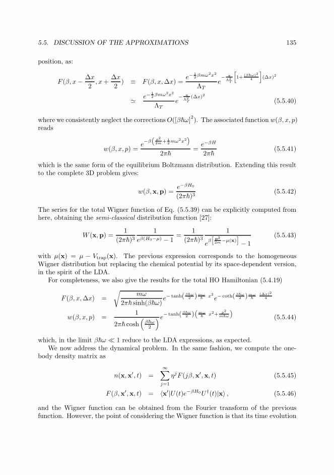
5.5. DISCUSSION OF THE APPROXIMATIONS 135
position, as:
F (β, x− ∆x
2, x+
∆x
2) ≡ F (β, x,∆x) =
e−12βmω2x2
ΛTe− π
Λ2T
[
1+(β~ω)2
4
]
(∆x)2
≃ e−12βmω2x2
ΛTe− π
Λ2T
(∆x)2
(5.5.40)
where we consistently neglect the correctionsO([β~ω]2). The associated function w(β, x, p)
reads
w(β, x, p) =e−β
(
p2
2m+ 12mω2x2
)
2π~=e−βH
2π~(5.5.41)
which is the same form of the equilibrium Boltzmann distribution. Extending this resultto the complete 3D problem gives:
w(β,x,p) =e−βH0
(2π~)3(5.5.42)
The series for the total Wigner function of Eq. (5.5.39) can be explicitly computed fromhere, obtaining the semi-classical distribution function [27]:
W (x,p) =1
(2π~)31
eβ(H0−µ) − 1=
1
(2π~)31
eβ[
p2
2m−µ(x)]
− 1
(5.5.43)
with µ(x) = µ − Vtrap(x). The previous expression corresponds to the homogeneousWigner distribution but replacing the chemical potential by its space-dependent version,in the spirit of the LDA.
For completeness, we also give the results for the total HO Hamiltonian (5.4.19)
F (β, x,∆x) =
√
mω
2π~ sinh(β~ω)e− tanh(β~ω
2 )mω~
x2
e− coth(β~ω2 )mω
~
(∆x)2
4
w(β, x, p) =1
2π~ cosh(
β~ω2
)e− tanh(β~ω
2 )(
mω~
x2+ p2
m~ω
)
(5.5.44)
which, in the limit β~ω ≪ 1 reduce to the LDA expressions, as expected.We now address the dynamical problem. In the same fashion, we compute the one-
body density matrix as
n(x,x′, t) =
∞∑
j=1
ηjF (jβ,x′,x, t) (5.5.45)
F (β,x′,x, t) = 〈x′|U(t)e−βH0U †(t)|x〉 , (5.5.46)
and the Wigner function can be obtained from the Fourier transform of the previousfunction. However, the point of considering the Wigner function is that its time evolution

136 CHAPTER 5. THERMAL DECAY IN A TRAPPED GAS
follows the differential equation
∂W
∂t+
p
m∇W −∇V ∇pW =
∞∑
n=1
∑
i1,i2...i2n+1
(−1)n~2n
22n(2n+ 1)!∇i1i2...i2n+1V∇i1i2...i2n+1
p W
∇i1i2...i2n+1p W ≡ ∂2n+1W
∂pi1∂pi2 . . . ∂pi2n+1
(5.5.47)
with V the total potential acting on the particles. We note that the l.h.s. of the previousequation is precisely the non-interacting Boltzmann equation of Eq. (5.3.1) and the r.h.s.introduces the quantum physics of ~. Interestingly, the time evolution of the Wignerfunction in a harmonic potential satisfies exactly the Boltzmann equation as the r.h.s.vanishes. As a consequence, the only possible quantum corrections in the dynamics arisefrom the Bragg pulse. The relative magnitude of the quantum corrections is O(~2k2/p2T )so they become negligible whenever Eq. (5.4.63) is fulfilled. Precisely, this conditionappeared in Sec. 5.4.4 as the condition for the smallness of the quantum corrections in~ to the classical result, in agreement with the discussion here presented. Its physicalmeaning is that the momentum of the photon has to be much smaller than the typicalmomentum of the particles, ~k ≪ pT . We can further evaluate this condition using theexperimental values presented at the beginning of this section. Since kl ∼ 1, Eq. (5.4.63)gives
~k
pT∼ kΛT ∼ N− 1
6 ≪ 1 (5.5.48)
as we are dealing with large numbers of particles N ∼ 104 − 107 and T ∼ T 0c . The above
equation provides a similar interpretation to the LDA: the scale of variation of the latticehas to be much larger than the associated thermal de Broglie wavelength.
From all the above considerations, we conclude that, as long as interactions are neg-ligible, if the cloud has a sufficiently large number of particles, the Wigner function andthe Boltzmann distribution function evolve with the same (classical) differential equation.Moreover, a large number of particles also implies that the LDA is valid, so one can usethe semi-classical distribution function of Eq. (5.5.43). In this way, quantum featuresenter only through the Bose statistics but not through the time-evolution of the particles,as their distribution obeys the classical Boltzmann equation.
5.6 Extension of the model
The theoretical model presented in the previous sections has shown that, whenever theconsidered approximations are valid, the introduction of a short Bragg pulse in a trappedcloud induces decaying oscillations in the spatial density profile. However, as we shownow, this result is in fact more general than the previous scenario. In order to address theproblem, we use the quantum description and keep assuming that the LDA is valid andinteractions do not play any dynamical role, see Secs. 5.5.1-5.5.2. In this non-interactingpicture, as the trapping potential does not enter into the dynamics, the problem is reducedto compute the time-evolution of a plane wave along the z-axis as given by Eq. (5.4.49).Since in this regime the motion after the pulse is the free one, we only need to compute

5.6. EXTENSION OF THE MODEL 137
the time evolution operator during the pulse, Uτ , given by Eq. (5.4.45). However, insteadof making use of the split-step approximation, we study more general situations. Inparticular, we first use the Dirac (or interaction) picture to compute the perturbativeseries for Uτ and after that we consider its formal expression for the general case.
5.6.1 Dirac picture
During the pulse, the motion along the z coordinate is governed (in the LDA) by theHamiltonian
Hz = H0z + V (z), H0z =P 2z
2m, (5.6.1)
with V (z) the potential created by the pulse. In order to solve the correspondingSchrodinger equation, we make use of the so-called Dirac picture, consisting in an uni-
tary transformation of the operators AD ≡ eiH0z~
tAe−iH0z~
t, with A an arbitrary quantumoperator. This implies that the time-evolution operator in the Dirac picture satisfies thedifferential equation:
V D(t)UDz (t) = i~
dUDz (t)
dt(5.6.2)
which can be simply integrated iteratively
UDz (t) = 1− i
~
∫ t
0
dt′ V D(t′)UDz (t′) =
∞∑
n=0
(−i~
)n ∫ t
0
dt1
∫ t1
0
dt2 . . .
∫ tn−1
0
dtn VD(t1) . . . V
D(tn)
(5.6.3)
In particular, for t = τ , we obtain Uτ = e−iH0z~
τUDz (τ). Comparing with Eq. (5.5.30), we
see that Gτ is an unitary transformation of UDz (τ) and is given by a similar expression
Gτ = e−iH0z~
τ2 UD
z (τ)eiH0z~
τ2 =
∞∑
n=0
(
− i
~
)n ∫ τ2
− τ2
dt1
∫ t1
− τ2
dt2 . . .
∫ tn−1
− τ2
dtn VD(t1) . . . V
D(tn)
(5.6.4)As a consequence, in analogy with Eq. (5.4.51), we rewrite the total evolution operatoras
Uz(t) = e−iH0z~
tGτ (5.6.5)
which we note that it is an exact relation for Uz(t) (apart from the trivial evolution factor
e−iH0z~
τ2 that we neglect as it does not enter into the dynamics). As argued in Sec. 5.5.3,
for a short pulse, Gτ ≃ eiu cos(kz) with corrections O(τ3). This result is easily recoveredwithin this picture by supposing that the time dependence of V D(t) is very weak andhence V D(t) ≃ V (z). Under this assumption, we get
Gτ ≃∞∑
n=0
(
−iV (z)τ~
)n
n!= e−iV (z)τ
~ (5.6.6)
We can try to understand this approximation by computing explicitly the matrix elementsof the first and second order terms of the previous perturbative series. After replacing
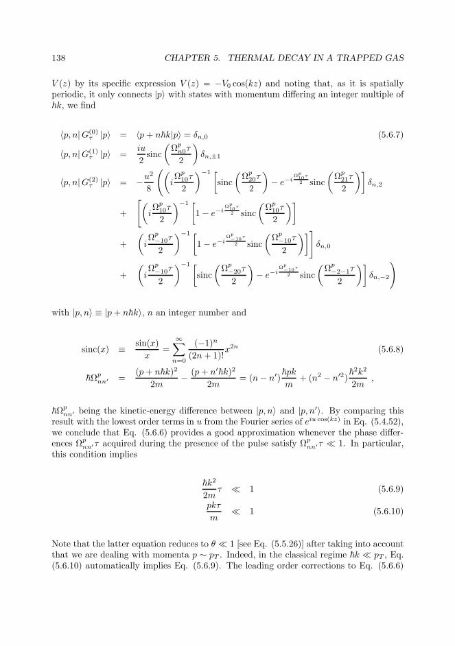
138 CHAPTER 5. THERMAL DECAY IN A TRAPPED GAS
V (z) by its specific expression V (z) = −V0 cos(kz) and noting that, as it is spatiallyperiodic, it only connects |p〉 with states with momentum differing an integer multiple of~k, we find
〈p, n|G(0)τ |p〉 = 〈p+ n~k|p〉 = δn,0 (5.6.7)
〈p, n|G(1)τ |p〉 =
iu
2sinc
(
Ωpn0τ
2
)
δn,±1
〈p, n|G(2)τ |p〉 = −u
2
8
(
(
iΩp
10τ
2
)−1 [
sinc
(
Ωp20τ
2
)
− e−iΩp10
τ
2 sinc
(
Ωp21τ
2
)]
δn,2
+
[
(
iΩp
10τ
2
)−1 [
1− e−iΩp10τ
2 sinc
(
Ωp10τ
2
)]
+
(
iΩp
−10τ
2
)−1 [
1− e−iΩp−10
τ
2 sinc
(
Ωp−10τ
2
)]
]
δn,0
+
(
iΩp
−10τ
2
)−1 [
sinc
(
Ωp−20τ
2
)
− e−iΩp−10
τ
2 sinc
(
Ωp−2−1τ
2
)]
δn,−2
)
with |p, n〉 ≡ |p+ n~k〉, n an integer number and
sinc(x) ≡ sin(x)
x=
∞∑
n=0
(−1)n
(2n+ 1)!x2n (5.6.8)
~Ωpnn′ =
(p+ n~k)2
2m− (p+ n′~k)2
2m= (n− n′)
~pk
m+ (n2 − n′2)
~2k2
2m,
~Ωpnn′ being the kinetic-energy difference between |p, n〉 and |p, n′〉. By comparing this
result with the lowest order terms in u from the Fourier series of eiu cos(kz) in Eq. (5.4.52),we conclude that Eq. (5.6.6) provides a good approximation whenever the phase differ-ences Ωp
nn′τ acquired during the presence of the pulse satisfy Ωpnn′τ ≪ 1. In particular,
this condition implies
~k2
2mτ ≪ 1 (5.6.9)
pkτ
m≪ 1 (5.6.10)
Note that the latter equation reduces to θ ≪ 1 [see Eq. (5.5.26)] after taking into accountthat we are dealing with momenta p ∼ pT . Indeed, in the classical regime ~k ≪ pT , Eq.(5.6.10) automatically implies Eq. (5.6.9). The leading order corrections to Eq. (5.6.6)
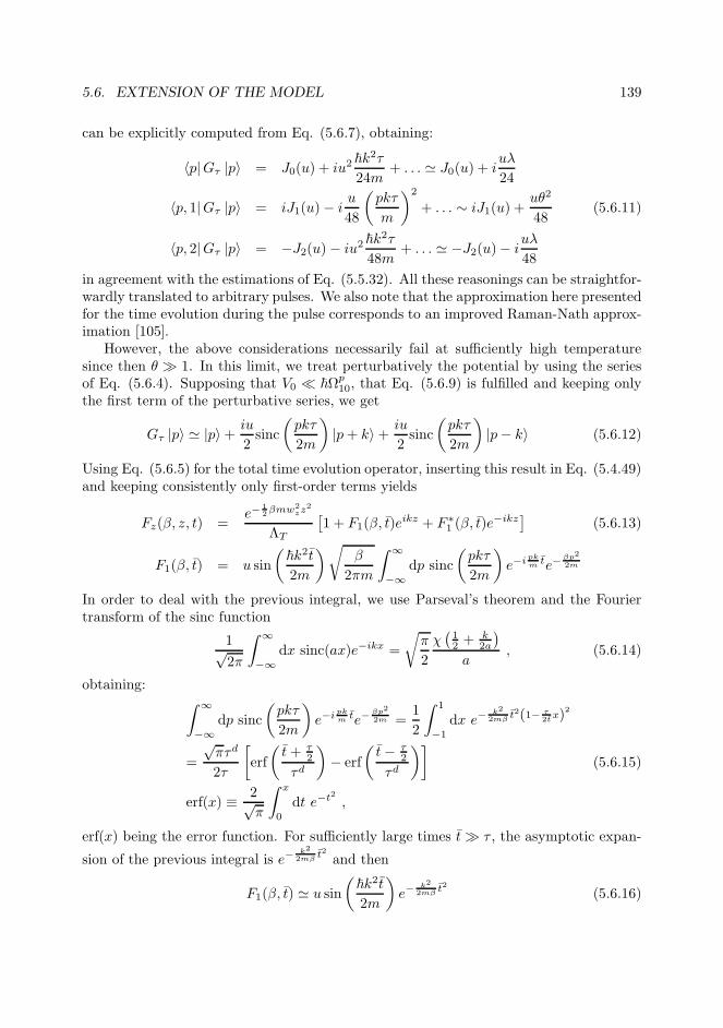
5.6. EXTENSION OF THE MODEL 139
can be explicitly computed from Eq. (5.6.7), obtaining:
〈p|Gτ |p〉 = J0(u) + iu2~k2τ
24m+ . . . ≃ J0(u) + i
uλ
24
〈p, 1|Gτ |p〉 = iJ1(u)− iu
48
(
pkτ
m
)2
+ . . . ∼ iJ1(u) +uθ2
48(5.6.11)
〈p, 2|Gτ |p〉 = −J2(u)− iu2~k2τ
48m+ . . . ≃ −J2(u)− i
uλ
48
in agreement with the estimations of Eq. (5.5.32). All these reasonings can be straightfor-wardly translated to arbitrary pulses. We also note that the approximation here presentedfor the time evolution during the pulse corresponds to an improved Raman-Nath approx-imation [105].
However, the above considerations necessarily fail at sufficiently high temperaturesince then θ ≫ 1. In this limit, we treat perturbatively the potential by using the seriesof Eq. (5.6.4). Supposing that V0 ≪ ~Ωp
10, that Eq. (5.6.9) is fulfilled and keeping onlythe first term of the perturbative series, we get
Gτ |p〉 ≃ |p〉+ iu
2sinc
(
pkτ
2m
)
|p+ k〉+ iu
2sinc
(
pkτ
2m
)
|p− k〉 (5.6.12)
Using Eq. (5.6.5) for the total time evolution operator, inserting this result in Eq. (5.4.49)and keeping consistently only first-order terms yields
Fz(β, z, t) =e−
12βmw2
zz2
ΛT
[
1 + F1(β, t)eikz + F ∗
1 (β, t)e−ikz
]
(5.6.13)
F1(β, t) = u sin
(
~k2t
2m
)
√
β
2πm
∫ ∞
−∞dp sinc
(
pkτ
2m
)
e−i pkm
te−βp2
2m
In order to deal with the previous integral, we use Parseval’s theorem and the Fouriertransform of the sinc function
1√2π
∫ ∞
−∞dx sinc(ax)e−ikx =
√
π
2
χ(
12 + k
2a
)
a, (5.6.14)
obtaining:∫ ∞
−∞dp sinc
(
pkτ
2m
)
e−i pkm
te−βp2
2m =1
2
∫ 1
−1
dx e−k2
2mβt2(1− τ
2tx)2
=
√πτd
2τ
[
erf
(
t+ τ2
τd
)
− erf
(
t− τ2
τd
)]
(5.6.15)
erf(x) ≡ 2√π
∫ x
0
dt e−t2 ,
erf(x) being the error function. For sufficiently large times t≫ τ , the asymptotic expan-
sion of the previous integral is e−k2
2mβt2 and then
F1(β, t) ≃ u sin
(
~k2t
2m
)
e−k2
2mβt2 (5.6.16)
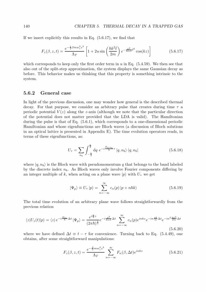
140 CHAPTER 5. THERMAL DECAY IN A TRAPPED GAS
If we insert explicitly this results in Eq. (5.6.17), we find that
Fz(β, z, t) =e−
12βmw2
zz2
ΛT
[
1 + 2u sin
(
~k2t
2m
)
e−k2
2mβt2 cos(kz)
]
(5.6.17)
which corresponds to keep only the first order term in u in Eq. (5.4.59). We then see thatalso out of the split-step approximation, the system displays the same Gaussian decay asbefore. This behavior makes us thinking that this property is something intrinsic to thesystem.
5.6.2 General case
In light of the previous discussion, one may wonder how general is the described thermaldecay. For that purpose, we consider an arbitrary pulse that creates during time τ aperiodic potential V (z) along the z-axis (although we note that the particular directionof the potential does not matter provided that the LDA is valid). The Hamiltonianduring the pulse is that of Eq. (5.6.1), which corresponds to a one-dimensional periodicHamiltonian and whose eigenfunctions are Bloch waves (a discussion of Bloch solutionsin an optical lattice is presented in Appendix E). The time evolution operators reads, interms of these eigenfunctions, as:
Uτ =∑
nb
∫ k2
− k2
dq e−iEq,nb
~τ |q, nb〉 〈q, nb| (5.6.18)
where |q, nb〉 is the Bloch wave with pseudomomentum q that belongs to the band labeledby the discrete index nb. As Bloch waves only involve Fourier components differing byan integer multiple of k, when acting on a plane wave |p〉 with Uτ we get
|Ψp〉 ≡ Uτ |p〉 =∞∑
n=−∞cn(p) |p+ n~k〉 (5.6.19)
The total time evolution of an arbitrary plane wave follows straightforwardly from theprevious relation
〈z|Uz(t)|p〉 = 〈z| e−iH0z~
∆t |Ψp〉 =ei
p~z
(2π~)12
e−i p2
2m~∆t
∞∑
n=−∞cn(p)e
inkze−in pkm
∆te−in2 ~k2
2m ∆t
(5.6.20)where we have defined ∆t ≡ t − τ for convenience. Turning back to Eq. (5.4.49), oneobtains, after some straightforward manipulations:
Fz(β, z, t) =e−
β2 mw2
zz2
ΛT
∞∑
n=−∞Fn(β,∆t)e
inkz (5.6.21)
5.7. EXPERIMENTAL DATA 141
with
Fn(β,∆t) =
√
β
2πm
∫ ∞
−∞dp fn(p,∆t)e
−in pkm
∆te−βp2
2m
fn(p,∆t) ≡∞∑
n′=−∞cn′(p)c∗n′−n(p)e
−i(2nn′−n2)~k2
2m ∆t (5.6.22)
Operating in the same fashion of Eq. (5.6.15)
Fn(β,∆t) =1√2π
∫ ∞
−∞dx fn(x,∆t)e
− n2k2
2mβ∆t2(1− m
k∆tx)2
fn(x,∆t) =1√2π
∫ ∞
−∞dp fn(p,∆t)e
−ipx (5.6.23)
with fn the Fourier transform of f(p,∆t). Once more, for sufficiently large times, theprevious integral gives
Fn(β,∆t) ≃ fn(0,∆t)e−n2k2
2mβ∆t2 (5.6.24)
which is the same asymptotic decaying behavior for the Fourier components of the maintheoretical model. Thus, this thermal decay is a general feature of a trapped gas of bosonswithin the approximated regime here considered (LDA and non-interacting dynamics).
The previous theoretical model can be further extended to the thermal componentfor temperatures below Tc since in the regime TTF < T < Tc the excitations of theuncondensed cloud are free particles to a good approximation [26, 27]. The temperatureTTF is the temperature associated to the Thomas-Fermi chemical potential µTF = kBTTF
µTF =~ω
2
(
15Nas
l
)25
(5.6.25)
Moreover, under the same general assumptions, the previous calculations can also betranslated to a fermion gas at sufficiently high temperature, where η . 1.
5.7 Experimental data
Here, we compare the previous theoretical calculations with the experimental data pro-vided by the Technion group for a setup similar to that of our model. It consists of aconfined thermal cloud of atoms of N 87Rb atoms (the same element of the simulationsof Chapter 2) with N ∼ 105− 106 ≫ 1 and trap frequencies ωx = ωy = ωr = 2π× 224 Hzand ωz = 2π×26 Hz. The mass of the atoms is the same as in Sec. 2.4, m = 1.44×10⁻²⁵
kg. Suddenly, it is introduced a short Bragg pulse of the same form of that of Eq. (5.2.2)with parameters V0 = 2.85 × 10⁻³⁰J, τ = 1.10 × 10⁻⁴s and k = 1.43 × 10⁶ m−1. Thepulse induces a periodic pattern in the density (which can be observed in Fig. 5.2) thateventually decays to the equilibrium configuration.

142 CHAPTER 5. THERMAL DECAY IN A TRAPPED GAS
Figure 5.2: Experimental in situ image of a thermal trapped cloud 0.07 ms after the pulse.This plot has been provided by Technion group.
Before of applying our theoretical model, we evaluate the relevant parameters of thesystem in order to check the considered approximations. The HO lengths are
lr =
√
~
mωr= 7.21× 10⁻⁷ m
lz =
√
~
mωz= 2.11× 10⁻⁶ m (5.7.1)
l =
√
~
mω= 1.03× 10⁻⁶ m

5.7. EXPERIMENTAL DATA 143
while we find, from Eqs. (5.5.1)-(5.5.3), that
T 0c = 4.93× 10⁻⁷ ×
(
N
106
)13
K ∼ 10−7 K
ΛT = 5.92× 10⁻⁷
√
10−7
T [K]m ∼ 10−7 m (5.7.2)
τd ∼ 10−4 s ∼ τ
We first analyze the validity of the LDA. Following the discussion of Sec. 5.5.1, thestatic LDA is valid when the relative finite-size shift of the critical temperature is small.This condition is fulfilled in our configuration as
δTcT 0c
= −0.73ωm
ωN− 1
3 ∼ 0.01 ≪ 1 (5.7.3)
On the other hand, the dynamic LDA is also a good approximation since τd ∼ τ and, asestimated after Eq. (5.5.15), ωzτ
d ∼√β~ωz ∼ 0.02 ≪ 1. In order to quantify interactions
between particles, we use the value of the scattering length for 87Rb, given in Sec. 2.4,as ∼ 100a0 = 5.29 nm. Interactions in the equilibrium configuration originate a shift inthe critical temperature given by Eq. (5.5.22)
δTcT 0c
= −1.32N16as
l∼ 0.07 (5.7.4)
which represents a small correction and consequently interactions can be treated to firstorder in a HFB approach, as done in Sec. 5.5.2. Also, as the LDA is valid, the mean-fieldHFB potential does not enter into the dynamics and only acts as an envelope. In respectto the collisional rate, we find from Eq. (5.5.24) that for T ∼ T 0
c
τd
τcol∼ a2s
Λ2T
d
ΛT∼ 5× 10⁻³ ≪ 1 (5.7.5)
Thus, we are safely in the non-interacting picture considered in the theory. In respectto the approximations for the motion during the pulse of Sec. 5.5.3, the dimensionlessimpulse parameter u of Eq. (5.4.46) is u = 2.97. The phase acquired during the pulsedue to the recoil energy is:
~k2
2mτ ≃ 0.08 ≪ 1 (5.7.6)
On the other hand, the dimensionless parameters of Eq. (5.5.26) are λ = 0.5 and θ & 1which are not strictly small. Nevertheless, the associated corrections (5.6.11) are indeedsmall:
uλ
24= 0.06,
uθ2
48& 0.1 (5.7.7)
Finally, we check that the classical picture for the motion of the particles is valid since
~k
pT∼ 0.1 (5.7.8)
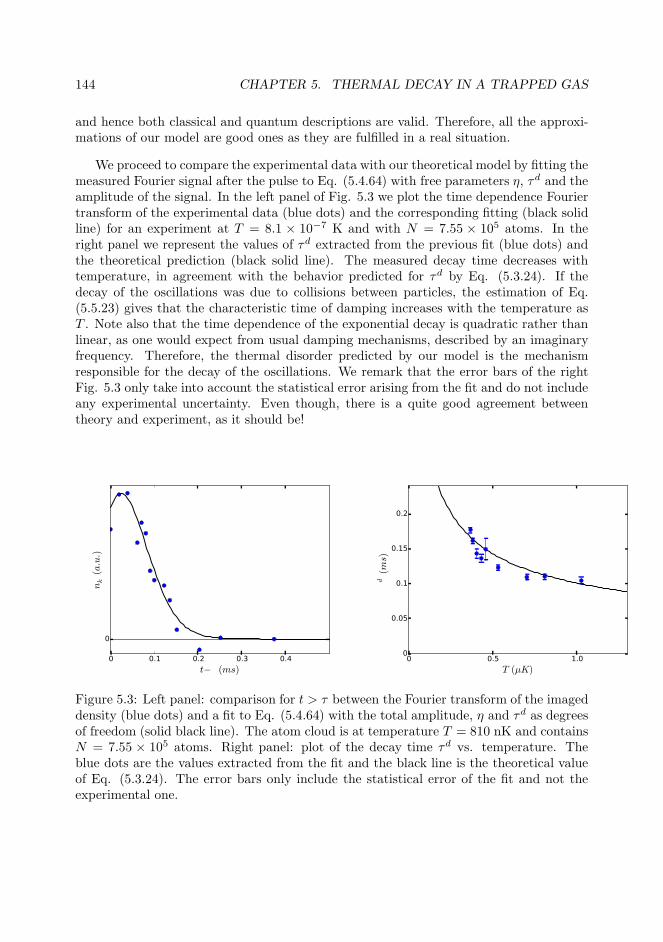
144 CHAPTER 5. THERMAL DECAY IN A TRAPPED GAS
and hence both classical and quantum descriptions are valid. Therefore, all the approxi-mations of our model are good ones as they are fulfilled in a real situation.
We proceed to compare the experimental data with our theoretical model by fitting themeasured Fourier signal after the pulse to Eq. (5.4.64) with free parameters η, τd and theamplitude of the signal. In the left panel of Fig. 5.3 we plot the time dependence Fouriertransform of the experimental data (blue dots) and the corresponding fitting (black solidline) for an experiment at T = 8.1 × 10⁻⁷ K and with N = 7.55 × 10⁵ atoms. In theright panel we represent the values of τd extracted from the previous fit (blue dots) andthe theoretical prediction (black solid line). The measured decay time decreases withtemperature, in agreement with the behavior predicted for τd by Eq. (5.3.24). If thedecay of the oscillations was due to collisions between particles, the estimation of Eq.(5.5.23) gives that the characteristic time of damping increases with the temperature asT . Note also that the time dependence of the exponential decay is quadratic rather thanlinear, as one would expect from usual damping mechanisms, described by an imaginaryfrequency. Therefore, the thermal disorder predicted by our model is the mechanismresponsible for the decay of the oscillations. We remark that the error bars of the rightFig. 5.3 only take into account the statistical error arising from the fit and do not includeany experimental uncertainty. Even though, there is a quite good agreement betweentheory and experiment, as it should be!
0 0.1 0.2 0.3 0.4
t−τ (ms)
0
nk (a.u.)
0 0.5 1.0
T (µK)
0
0.05
0.1
0.15
0.2
τd (ms)
Figure 5.3: Left panel: comparison for t > τ between the Fourier transform of the imageddensity (blue dots) and a fit to Eq. (5.4.64) with the total amplitude, η and τd as degreesof freedom (solid black line). The atom cloud is at temperature T = 810 nK and containsN = 7.55 × 10⁵ atoms. Right panel: plot of the decay time τd vs. temperature. Theblue dots are the values extracted from the fit and the black line is the theoretical valueof Eq. (5.3.24). The error bars only include the statistical error of the fit and not theexperimental one.

5.8. CONCLUSIONS AND OUTLOOK 145
5.8 Conclusions and outlook
We have proven that the introduction of a short Bragg pulse in a trapped thermal cloudinduces a periodic density pattern that, after the removal of the pulse, decays with aGaussian behavior. In particular, we have shown that this behavior is explained byboth classical and quantum descriptions of the problem and we have established the linkbetween the two formalisms. We have also checked that the approximations made forthe model are satisfied in typical setups. The physical origin of this decay is indeed asingle-particle phenomenon, arising from the thermal disorder of the particles, in contrastto the usual collisional damping mechanism of the collective modes. Finally, we havecompared the theoretical predictions with actual experimental data, finding a very goodagreement.
As argued in the main text, the obtained results can be extended to more generalsituations. In particular, as long as the local density approximation is valid and the roleof interactions can be neglected, the same behavior appears for an arbitrary spatiallyperiodic pulse. Mutatis mutandi, the theoretical model developed is translatable to othersimilar configurations such as the thermal component of a Bose gas at temperature TTF <T < Tc (with TTF the temperature of the Thomas-Fermi chemical potential) or a Fermigas at sufficiently high temperatures. A future computation could try to apply these ideasto the phonons above the condensate in the regime 0 < T < TTF .

146 CHAPTER 5. THERMAL DECAY IN A TRAPPED GAS

Part III
Quantum Hall effect on
graphene
147

Chapter 6Collective modes of the phase diagram
of the ν = 0 quantum Hall state
6.1 Introduction
We switch in the last part of the thesis to a very different system: electrons in grapheneunder the effect of a strong magnetic field. One of the main contrasts with the formerchapters arises from the fact that electrons are fermions. This implies that they obeythe Pauli exclusion principle so creation/annihilation operators anti-commute instead ofcommute. Besides, graphene is a two-dimensional system. We also have to deal withthe extra degrees of freedom corresponding to spin. Moreover, in graphene there areother extra degrees of freedom corresponding to valley and sublattice, originating a richstructure in the spectrum of excitations, as will be discussed.
We focus here on the ν = 0 quantum Hall (QH) state of bilayer graphene (BLG), inwhich the zero-energy Landau level (LL) is half-filled. Several works have been devotedto study its phase diagram, see for instance Refs. [106, 107, 108]. In particular, the latterreference [108] shows a complete study of the phase diagram by taking into account themost general spin symmetric interactions (including short-range valley/sublattice asym-metric interactions) and the introduction of a voltage between the two layers. The identi-fied phases are ferromagnetic (F), canted anti-ferromagnetic (CAF), fully layer-polarized(FLP) and partially layer-polarized (PLP) [109, 108]. The resulting phase diagram isanalog to that of monolayer graphene (MLG) [109] since the form of the short-range val-ley/sublattice asymmetric interactions is the same. On the other hand, some works havecomputed the collective modes of the ν = 0 QH state for both monolayer and bilayergraphene [110, 111, 112, 113, 114]; however, to our best knowledge, a computation of thecollective modes of the complete phase diagram of Ref. [109] using the full short-rangeHamiltonian has not been performed yet.
Thus, in this chapter we use the time-dependent Hartree-Fock approximation (TD-HFA) to compute, neglecting LL mixing, the collective modes of the ν = 0 QH phases of
149
150CHAPTER 6. COLLECTIVE MODES OF THE ν = 0 QUANTUM HALL STATE
Ref. [108]. We find that the short-range valley/sublattice interactions play a crucial rolein order to understand the stability of the different phases since for zero-momentum thelowest energy collective modes are independent of the Coulomb interaction strength. Inparticular, we prove that the boundary between the F and FLP phases presents a gaplessmode that arises from a residual U(1) symmetry, which can be regarded as a remanent ofthe full SO(5) symmetry existing for the same boundary at zero Zeeman energy in MLG[114]. A similar gapless mode appears in the boundary between the CAF and PLP phases.Besides, we show that the CAF and PLP phases can present dynamical instabilities anddiscuss possible experimental scenarios for their observation. Due to the strong analogybetween the ν = 0 QH states in bilayer and monolayer graphene, most of these resultsare straightforwardly translated to MLG. In this way, the work presented here providesa natural continuation of those of Refs. [108, 111, 112, 113, 114].
We first introduce the physical model for low energies of bilayer graphene in Sec. 6.2.We present in Sec. 6.3.1 the effective Hamiltonian considered in this work and re-derivein Sec. 6.3.2 the phase diagram of Ref. [108] within a Hartree-Fock mean-field scheme.The formalism of the TDHFA is presented in Sec. 6.4.1 and the dispersion relation of thedifferent collective modes is computed in Sec. 6.4.2. We translate the same calculationsto monolayer graphene in Sec. 6.5. We consider the effects of LL mixing in Sec. 6.6.Possible scenarios for the observation of the dynamical instabilities are discussed in Sec.6.7. The conclusions are given in Sec. 6.8. Technical details about the diagonalization ofthe Hartree-Fock equations and the TDHFA are given in Appendices J-K.
6.2 Physical model of bilayer graphene
In the first place, we briefly review the main details of the effective model of bilayergraphene at low energies. For more details on the Hamiltonian of monolayer and bilayergraphene in the presence of a magnetic field, see for instance Refs. [115, 109].
In this approximation, the field operator for the electrons has 8 components and reads:
ψ(x) =
[
ψ+(x)
ψ−(x)
]
ψσ(x) =
ψKAσ(x)
ψKBσ(x)
ψK′Bσ(x)
ψK′Aσ(x)
≡
ψKAσ(x)
ψKBσ(x)
ψK′Aσ(x)
ψK′Bσ(x)
, σ = ± (6.2.1)
where A, B represent the most far apart sublattices, K,K ′ the two valleys and σ thespin polarization. We note that the two sublattices are interchanged in the K ′ valleyso, as usually done, we will refer to the corresponding subspace as AB in order to avoidconfusions. The 8 components of the field operator then correspond to the total subspaceKK ′ ⊗ AB ⊗ s, s being the spin subspace. As electrons are fermions, the componentsµ, ν of the field operator obey the canonical anti-commutation rules:
ψµ(x), ψν (x′)
= δµνδ(x− x′) (6.2.2)
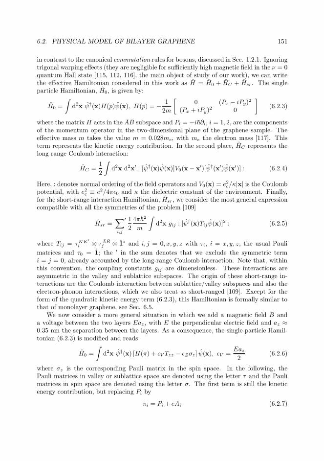
6.2. PHYSICAL MODEL OF BILAYER GRAPHENE 151
in contrast to the canonical commutation rules for bosons, discussed in Sec. 1.2.1. Ignoringtrigonal warping effects (they are negligible for sufficiently high magnetic field in the ν = 0quantum Hall state [115, 112, 116], the main object of study of our work), we can writethe effective Hamiltonian considered in this work as H = H0 + HC + Hsr. The singleparticle Hamiltonian, H0, is given by:
H0 =
∫
d2x ψ†(x)H(p)ψ(x), H(p) = − 1
2m
[
0 (Px − iPy)2
(Px + iPy)2 0
]
(6.2.3)
where the matrixH acts in the AB subspace and Pi = −i~∂i, i = 1, 2, are the componentsof the momentum operator in the two-dimensional plane of the graphene sample. Theeffective mass m takes the value m = 0.028me, with me the electron mass [117]. Thisterm represents the kinetic energy contribution. In the second place, HC represents thelong range Coulomb interaction:
HC =1
2
∫
d2x d2x′ : [ψ†(x)ψ(x)]V0(x− x′)[ψ†(x′)ψ(x′)] : (6.2.4)
Here, : denotes normal ordering of the field operators and V0(x) = e2c/κ|x| is the Coulombpotential, with e2c ≡ e2/4πǫ0 and κ the dielectric constant of the environment. Finally,for the short-range interaction Hamiltonian, Hsr, we consider the most general expressioncompatible with all the symmetries of the problem [109]
Hsr =∑′
i,j
1
2
4π~2
m
∫
d2x gij : [ψ†(x)Tij ψ(x)]
2 : (6.2.5)
where Tij = τKK′i ⊗ τ AB
j ⊗ 1s and i, j = 0, x, y, z with τi, i = x, y, z, the usual Pauli
matrices and τ0 = 1; the ′ in the sum denotes that we exclude the symmetric termi = j = 0, already accounted by the long-range Coulomb interaction. Note that, withinthis convention, the coupling constants gij are dimensionless. These interactions areasymmetric in the valley and sublattice subspaces. The origin of these short-range in-teractions are the Coulomb interaction between sublattice/valley subspaces and also theelectron-phonon interactions, which we also treat as short-ranged [109]. Except for theform of the quadratic kinetic energy term (6.2.3), this Hamiltonian is formally similar tothat of monolayer graphene, see Sec. 6.5.
We now consider a more general situation in which we add a magnetic field B anda voltage between the two layers Eaz , with E the perpendicular electric field and az ≈0.35 nm the separation between the layers. As a consequence, the single-particle Hamil-tonian (6.2.3) is modified and reads
H0 =
∫
d2x ψ†(x) [H(π) + ǫV Tzz − ǫZσz ] ψ(x), ǫV =Eaz2
(6.2.6)
where σz is the corresponding Pauli matrix in the spin space. In the following, thePauli matrices in valley or sublattice space are denoted using the letter τ and the Paulimatrices in spin space are denoted using the letter σ. The first term is still the kineticenergy contribution, but replacing Pi by
πi = Pi + eAi (6.2.7)

152CHAPTER 6. COLLECTIVE MODES OF THE ν = 0 QUANTUM HALL STATE
The second term arises from the voltage difference between the two layers. The third term
takes into account the Zeeman effect with ǫZ = µBB,B =√
B2‖ +B2
⊥. Here, we assume
that the magnetic field is not necessarily in the z direction, i.e., it can present a parallelcomponent to the graphene plane B = [B‖ cosφB , B‖ sinφB , B⊥]. The polarizationsσ = ± correspond to the spin components that are antiparallel (parallel) to the totalmagnetic field B, respectively. We may define the operator
aB =lB~
πy + iπx√2
, lB =
√
~
eB⊥=
25.7√
B⊥[T]nm, (6.2.8)
lB being the magnetic length. This operator is an annihilation-type operator that satisfiesthe usual commutation rule [aB, a
†B] = 1, similar to that of the harmonic oscillator Hamil-
tonian discussed in Sec. 5.4.3. The kinetic energy term of Eq. (6.2.6) is then rewritten
in terms of aB, a†B as
H(π) = ~ωB
[
0 a2B(a†B)
2 0
]
, ωB =eB⊥m
= 1.76×10¹¹me
mB⊥[T] Hz = 6.28×10¹²B⊥ Hz
(6.2.9)Taking into account that only the perpendicular magnetic field affects the orbital motionand using the Landau gauge, we can write the potential vector in Eq. (6.2.7) as A(x) =[0, B⊥x, 0]. In this particular gauge, the eigenstates the operator (6.2.9) are characterizedby the following quantum numbers: the magnetic index n, which is an integer numberand characterizes the energy of the corresponding Landau level, ǫn, the momentum inthe y-direction k and the polarization in the KK ′ ⊗ s subspace α. Specifically, they aregiven by Ψ0
n,k,α(x) = Ψ0n,k(x)χα, where χα is an arbitrary 4-component spinor in the
valley-spin subspace and the orbital wave function with components in the subspace ABis
Ψ0n,k(x) =
eiky√
Ly
1√2
[
sgn n φ|n|−2(x+ kl2B)φ|n|(x+ kl2B)
]
, ǫn = sgn n√
|n|(|n| − 1)~ωB (6.2.10)
for |n| 6= 0, 1 and
Ψ0n,k(x) =
eiky√
Ly
[
0φ|n|(x+ kl2B)
]
, ǫn = 0 (6.2.11)
for the degenerate levels |n| = 0, 1 with zero energy (note that n = ±1 are indeed thesame state). Hereafter, we refer to this manifold of states as the ZLL (zero Landau level).In the previous equations, Ly is the length of the system in the y direction and φn(x) isthe usual harmonic oscillator wave function, see Eq. J.1.2 for its explicit expression. Thekinetic energy does not depend on the polarization χα as it is degenerate in that sub-space. Interestingly, the wave functions in the ZLL only have non-vanishing componentsin the subspace KK ′ ⊗ B ⊗ s. The field operator is decomposed in terms of the previouseigenfunctions as
ψ(x) =
∞∑′
n=−∞
∑
k,α
Ψ0n,k,α(x)cn,k,α (6.2.12)
where ′ means that n takes every integer value except n = −1.
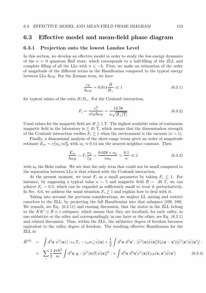
6.3. EFFECTIVE MODEL AND MEAN-FIELD PHASE DIAGRAM 153
6.3 Effective model and mean-field phase diagram
6.3.1 Projection onto the lowest Landau Level
In this section, we develop an effective model in order to study the low-energy dynamicsof the ν = 0 quantum Hall state, which corresponds to a half-filling of the ZLL andcomplete filling of all the LLs with n ≤ −2. First, we make an estimation of the orderof magnitude of the different terms in the Hamiltonian compared to the typical energybetween LLs ~ωB. For the Zeeman term, we have
ǫZ~ωB
= 0.014B
B⊥≪ 1 (6.3.1)
for typical values of the ratio B/B⊥. For the Coulomb interaction,
Fc =e2c
κlB~ωB=
13.58
κ√
B⊥[T](6.3.2)
Usual values for the magnetic field are B & 1 T. The highest available value of continuousmagnetic field in the laboratory is . 45 T, which means that the dimensionless strengthof the Coulomb interaction verifies Fc & 1 when the environment is the vacuum (κ = 1).
Finally, a dimensional analysis of the short-range terms gives an order of magnitudeestimate Esr ∼ e2caL/κl
2B with aL ≈ 0.14 nm the nearest-neighbor constant. Then:
Esr
~ωB∼ Fc
aLlB
=0.028× aL
κa0≃ 0.1
κ≪ 1 (6.3.3)
with a0 the Bohr radius. We see that the only term that could not be small compared tothe separation between LLs is that related with the Coulomb interaction.
At the present moment, we treat Fc as a small parameter by taking Fc . 1. Forinstance, by supposing a typical value κ ∼ 5 and magnetic field B ∼ 20 T , we canachieve Fc ∼ 0.5, which can be regarded as sufficiently small to treat it perturbatively.In Sec. 6.6, we address the usual situation Fc & 1 and explain how to deal with it.
Taking into account the previous considerations, we neglect LL mixing and restrictourselves to the ZLL, by projecting the full Hamiltonian into that subspace [109, 108].We remark, see Eq. (6.2.11) and ensuing discussion, that the states in the ZLL belongto the KK ′ ⊗ B ⊗ s subspace, which means that they are localized, for each valley, inone sublattice or the other and correspondingly, in one layer or the other; see Eq. (6.2.1)and related discussion. Thus, within the ZLL, the sublattice degree of freedom becomesequivalent to the valley degree of freedom. The resulting effective Hamiltonian for theZLL is:
H(0) =
∫
d2x ψ†(x) [−ǫV Tz − ǫZσz ] ψ(x) +1
2
∫
d2x d2x′ : [ψ†(x)ψ(x)]V0(x − x′)[ψ†(x′)ψ(x′)] :
+∑
i
1
2
4π~2
m
∫
d2x gi : [ψ†(x)Tiψ(x)]
2 : +
∫
d2x d2x′ψ†(x)VDS(x,x′)ψ(x′) (6.3.4)
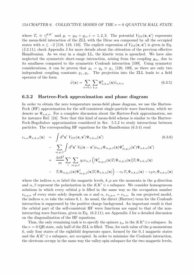
154CHAPTER 6. COLLECTIVE MODES OF THE ν = 0 QUANTUM HALL STATE
where Ti ≡ τKK′i and gi = gi0 + giz, i = 1, 2, 3. The potential VDS(x,x
′) representsthe mean-field interaction of the ZLL with the Dirac sea compound by all the occupiedstates with n ≤ −2 [118, 119, 116]. The explicit expression of VDS(x,x
′) is given in Eq.(J.2.11); check Appendix J for more details about the obtention of the previous effectiveHamiltonian. As we stay in a single LL, the kinetic term is quenched. We have alsoneglected the symmetric short-range interaction, arising from the coupling g0z, due toits smallness compared to the symmetric Coulomb interaction [109]. Using symmetryconsiderations, it can be proven that gx = gy ≡ g⊥ [120, 109], so there are only twoindependent coupling constants g⊥, gz. The projection into the ZLL leads to a fieldoperator of the form
ψ(x) =∑
n=0,1
∑
k,α
Ψ0n,k,α(x)cn,k,α (6.3.5)
6.3.2 Hartree-Fock approximation and phase diagram
In order to obtain the zero temperature mean-field phase diagram, we use the Hartree-Fock (HF) approximation for the self-consistent single-particle wave functions, which wedenote as Ψn,k,α. For a complete discussion about the Hartree-Fock approximation, seefor instance Ref. [24]. Note that this kind of mean-field scheme is similar to the Hartree-Fock-Bogoliubov approximation considered in Sec. 5.5.2 to study interactions betweenparticles. The corresponding HF equations for the Hamiltonian (6.3.4) read
ǫn,αΨn,k,α(x) =
∫
d2x′ VDS(x,x′)Ψn,k,α(x
′) (6.3.6)
−∑
m,p,β
∫
d2x′ V0(x− x′)νm,βΨm,p,β(x)Ψ†m,p,β(x
′)Ψn,k,α(x′)
+4π~2
m
∑
i
∑
m,p,β
giνm,β
(
[Ψ†m,p,β(x)TiΨm,p,β(x)]TiΨn,k,α(x)
− TiΨm,p,β(x)Ψ†m,p,β(x)TiΨn,k,α(x)
)
− ǫV TzΨn,k,α(x) − ǫZσzΨn,k,α(x)
where the indices n,m label the magnetic levels, k, p are the momenta in the y-directionand α, β represent the polarization in the KK ′ ⊗ s subspace. We consider homogeneoussolutions in which every orbital p is filled in the same way so the occupation numberνn,p,α of every state solely depends on n and α, νn,p,α = νn,α. In our projected model,the indices n,m take the values 0, 1. As usual, the direct (Hartree) term for the Coulombinteraction is suppressed by the positive charge background. An important result is thatthe orbital part of the self-consistent HF wave functions are equal to that of the non-interacting wave functions, given in Eq. (6.2.11); see Appendix J for a detailed discussionon the diagonalization of the HF equations.
Thus, the only remaining task is to specify the spinors χα in the KK ′⊗s subspace. Inthe ν = 0 QH state, only half of the ZLL is filled. Thus, for each value of the y-momentumk, only four states of the eightfold degenerate space, formed by the 0, 1 magnetic statesand the KK ′ ⊗ s subspace, are occupied. In order to minimize the Coulomb interaction,the electrons occupy in the same way the valley-spin subspace for the two magnetic levels,
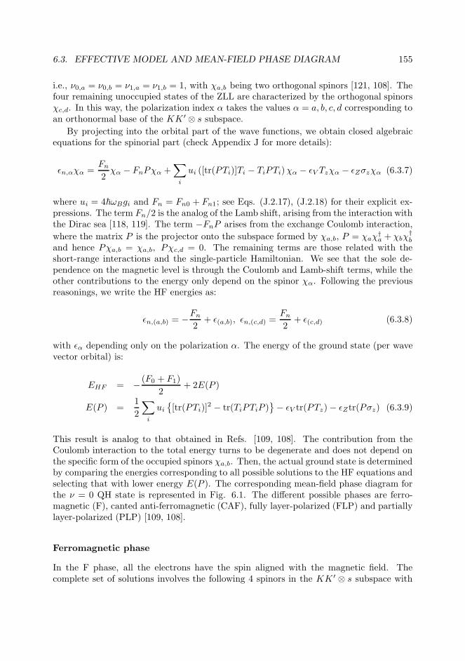
6.3. EFFECTIVE MODEL AND MEAN-FIELD PHASE DIAGRAM 155
i.e., ν0,a = ν0,b = ν1,a = ν1,b = 1, with χa,b being two orthogonal spinors [121, 108]. Thefour remaining unoccupied states of the ZLL are characterized by the orthogonal spinorsχc,d. In this way, the polarization index α takes the values α = a, b, c, d corresponding toan orthonormal base of the KK ′ ⊗ s subspace.
By projecting into the orbital part of the wave functions, we obtain closed algebraicequations for the spinorial part (check Appendix J for more details):
ǫn,αχα =Fn
2χα − FnPχα +
∑
i
ui ([tr(PTi)]Ti − TiPTi)χα − ǫV Tzχα − ǫZσzχα (6.3.7)
where ui = 4~ωBgi and Fn = Fn0 + Fn1; see Eqs. (J.2.17), (J.2.18) for their explicit ex-pressions. The term Fn/2 is the analog of the Lamb shift, arising from the interaction withthe Dirac sea [118, 119]. The term −FnP arises from the exchange Coulomb interaction,
where the matrix P is the projector onto the subspace formed by χa,b, P = χaχ†a + χbχ
†b
and hence Pχa,b = χa,b, Pχc,d = 0. The remaining terms are those related with theshort-range interactions and the single-particle Hamiltonian. We see that the sole de-pendence on the magnetic level is through the Coulomb and Lamb-shift terms, while theother contributions to the energy only depend on the spinor χα. Following the previousreasonings, we write the HF energies as:
ǫn,(a,b) = −Fn
2+ ǫ(a,b), ǫn,(c,d) =
Fn
2+ ǫ(c,d) (6.3.8)
with ǫα depending only on the polarization α. The energy of the ground state (per wavevector orbital) is:
EHF = − (F0 + F1)
2+ 2E(P )
E(P ) =1
2
∑
i
ui
[tr(PTi)]2 − tr(TiPTiP )
− ǫV tr(PTz)− ǫZtr(Pσz) (6.3.9)
This result is analog to that obtained in Refs. [109, 108]. The contribution from theCoulomb interaction to the total energy turns to be degenerate and does not depend onthe specific form of the occupied spinors χa,b. Then, the actual ground state is determinedby comparing the energies corresponding to all possible solutions to the HF equations andselecting that with lower energy E(P ). The corresponding mean-field phase diagram forthe ν = 0 QH state is represented in Fig. 6.1. The different possible phases are ferro-magnetic (F), canted anti-ferromagnetic (CAF), fully layer-polarized (FLP) and partiallylayer-polarized (PLP) [109, 108].
Ferromagnetic phase
In the F phase, all the electrons have the spin aligned with the magnetic field. Thecomplete set of solutions involves the following 4 spinors in the KK ′ ⊗ s subspace with
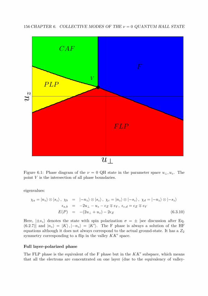
156CHAPTER 6. COLLECTIVE MODES OF THE ν = 0 QUANTUM HALL STATE
u⊥
uz
FLP
F
CAF
PLPV
Figure 6.1: Phase diagram of the ν = 0 QH state in the parameter space u⊥, uz. Thepoint V is the intersection of all phase boundaries.
eigenvalues:
χa = |nz〉 ⊗ |sz〉 , χb = |−nz〉 ⊗ |sz〉 , χc = |nz〉 ⊗ |−sz〉 , χd = |−nz〉 ⊗ |−sz〉ǫa,b = −2u⊥ − uz − ǫZ ∓ ǫV , ǫc,d = ǫZ ∓ ǫV
E(P ) = −(2u⊥ + uz)− 2ǫZ (6.3.10)
Here, |±sz〉 denotes the state with spin polarization σ = ± [see discussion after Eq.(6.2.7)] and |nz〉 = |K〉 , |−nz〉 = |K ′〉. The F phase is always a solution of the HFequations although it does not always correspond to the actual ground-state. It has a Z2
symmetry corresponding to a flip in the valley KK ′ space.
Full layer-polarized phase
The FLP phase is the equivalent of the F phase but in the KK ′ subspace, which meansthat all the electrons are concentrated on one layer (due to the equivalency of valley-
6.3. EFFECTIVE MODEL AND MEAN-FIELD PHASE DIAGRAM 157
sublattice-layer of the ZLL in BLG). The corresponding spinors are now:
χa = |nz〉 ⊗ |sz〉 , χb = |nz〉 ⊗ |−sz〉 , χc = |−nz〉 ⊗ |sz〉 , χd = |−nz〉 ⊗ |−sz〉ǫa,b = uz ∓ ǫZ − ǫV , ǫc,d = −2u⊥ − 2uz ∓ ǫZ + ǫV
E(P ) = uz − 2ǫV (6.3.11)
In analogy to the F phase, it is always a solution to the HF equations but not necessarilythe ground-state. It also has a Z2 symmetry corresponding to flip the spins. By comparingthe energies of the two phases, we can obtain the boundary between the F and FLP phases:
u⊥ + uz = ǫV − ǫZ (6.3.12)
Canted anti-ferromagnetic phase
The previous phases would be the only possible phases if there were not short-rangeinteractions, i.e., u⊥ = uz = 0. However, when taking into account these interactions, thesystem can exhibit canted anti-ferromagnetism or partially layer-polarization in order tominimize the interaction energy. In the CAF phase, we have that:
χa = |nz〉 ⊗ |sa〉 , χb = |−nz〉 ⊗ |sb〉 , χc = |nz〉 ⊗ |−sa〉 , χd = |−nz〉 ⊗ |−sb〉ǫa,b = −uz − 2u⊥ cos2 θs − ǫZ cos θs ∓ ǫV = −uz ∓ ǫV
ǫc,d = −2u⊥ sin2 θs + ǫZ cos θs ∓ ǫV = −2u⊥ ∓ ǫV
E(P ) = −uz − ǫZ cos θs (6.3.13)
where sa,b = [± sin θs cosφs,± sin θs sinφs, cos θs] and the tilting angle is cos θs = −ǫZ/2u⊥.As the azimut φs is a free parameter, we see that CAF phase has U(1) symmetry. Whenthis solutions exists, it always has lower energy than the regular F phase, hence thecondition for the presence of the CAF phase is just
cos θs < 1 ⇒ u⊥ < − ǫZ2
(6.3.14)
Partially layer-polarized phase
In analogy with the relation between the FLP and F phases, the PLP is similar to theCAF phase but in the valley subspace:
χa = |n〉 ⊗ |sz〉 , χb = |n〉 ⊗ |−sz〉 , χc = |−n〉 ⊗ |sz〉 , χd = |−n〉 ⊗ |−sz〉ǫa,b = u⊥ sin2 θv + uz cos
2 θv ∓ ǫZ − ǫV cos θv = u⊥ ∓ ǫZ
ǫc,d = −2u⊥ − uz − u⊥ sin2 θv − uz cos2 θv + ǫV cos θv ∓ ǫZ = −3u⊥ − uz ∓ ǫZ
E(P ) = u⊥ sin2 θv + uz cos2 θv − 2ǫV cos θv = u⊥ − ǫV cos θv (6.3.15)
with n = [sin θv cosφv, sin θv sinφv, cos θv] and cos θv = ǫv/(uz − u⊥). The PLP phasealso presents an U(1) symmetry. In analogy with the F-CAF phase transition, whenever
158CHAPTER 6. COLLECTIVE MODES OF THE ν = 0 QUANTUM HALL STATE
this solution exists, it has lower energy than the FLP phase. The existence condition forthe PLP phase is
cos θv < 1 ⇒ uz − u⊥ > ǫV (6.3.16)
On the other hand, the boundary between the FLP and the CAF phases is placed at
uz + u⊥ =ǫ2V
uz − u⊥+
ǫ2Z2u⊥
(6.3.17)
Critical point
The resulting phase diagram from this HF scheme, depicted in Fig. 6.1, is the same asthat of Ref. [108]. It is straightforward to show that all phase boundaries intersect at thecritical point
V = (u∗⊥, u∗z) = (−ǫZ/2, ǫV − ǫZ/2). (6.3.18)
As discussed in the previous section, we only need two parameters to characterize theasymmetric interaction, u⊥, uz. The expected phase for the ν = 0 QH state of bilayergraphene is the CAF phase at ǫV = 0 and zero in-plane component of the magneticfield [122, 123], which implies that uz > −u⊥ > 0. The exact values of these short-rangeenergies remain unknown but their order of magnitude is uz, |u⊥| ∼ 0.1~ωB [124, 114, 125].In the following, we treat them as phenomenological inputs for the theory. We note that,since u⊥ < 0, all the phases can be explored because, as Eq. 6.3.18 reveals, the criticalV point can be placed anywhere in the whole semi-plane u⊥ < 0 by just changing thein-plane component of the magnetic field or the layer voltage.
6.4 Collective modes
6.4.1 Correlation functions and the time-dependent Hartree-Fock
approximation
The collective mode frequencies are given by the poles of the set of correlation functions:
ΠA(x, x′) = −i 〈T ∆[ψ†(x)θ†Aψ(x)]∆[ψ†(x′)θAψ(x
′)]〉 (6.4.1)
where x = (x, t), T denotes time-ordering, all the expectation value are evaluated in theground state of the system and θA is an arbitrary operator in the valley-spin subspace.As in Sec. 3.3, ∆O = O − 〈O〉 denotes the fluctuations of an operator around its meanvalue.
The previous correlation functions are computed within the TDHFA. We now brieflypresent the diagrammatic formalism considered, following closely Refs. [126, 127]. The HFeigenfunctions and eigenvalues of Eq. (6.3.6) lead to the self-consistent Green’s functions:
Gµν(x,x′, ω) =∑
n,p,α
Ψµn,p,α(x)Ψ
ν∗n,p,α(x
′)Gn,α(ω) (6.4.2)
Gn,α(ω) =1− νn,α
ω − ωn,α + iη+
νn,αω − ωn,α − iη
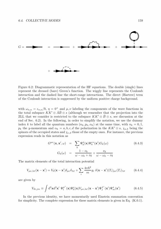
6.4. COLLECTIVE MODES 159
G = = + +
+
Figure 6.2: Diagrammatic representation of the HF equations. The double (single) linesrepresent the dressed (bare) Green’s function. The wiggly line represents the Coulombinteraction and the dashed line the short-range interactions. The direct (Hartree) termof the Coulomb interaction is suppressed by the uniform positive charge background.
with ωn,α = ǫn,α/~, η = 0+ and µ, ν labeling the components of the wave functions inthe total subspace KK ′ ⊗ AB ⊗ s (although we remember that the projection into theZLL that we consider is restricted to the subspace KK ′ ⊗ B ⊗ s, see discussion at theend of Sec. 6.2). In the following, in order to simplify the notation, we use the dummyindex k to label all the quantum numbers (nk, pk, αk) at the same time, with nk = 0, 1,pk the y-momentum and αk = a, b, c, d the polarization in the KK ′ ⊗ s, χa,b being thespinors of the occupied states and χc,d those of the empty ones. For instance, the previousexpression reads in this notation as
Gµν(x,x′, ω) =∑
k
Ψµk(x)Ψ
ν∗k (x′)Gk(ω) (6.4.3)
Gk(ω) =1− νk
ω − ωk + iη+
νkω − ωk − iη
The matrix elements of the total interaction potential
Vµν,λσ(x − x′) = V0(x− x′)δµνδλσ +∑
i
4π~2
mgi δ(x− x′)(Ti)µν(Ti)λσ (6.4.4)
are given by
Vlk,jm ≡∫
d2xd2x′ Ψµ∗
l (x)Ψνk(x)Vµν,λσ(x− x′)Ψλ∗
j (x′)Ψσm(x′) (6.4.5)
In the previous identity, we have momentarily used Einstein summation conventionfor simplicity. The complete expression for these matrix elements is given in Eq. (K.0.1).
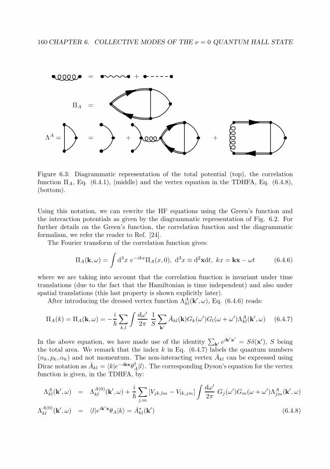
160CHAPTER 6. COLLECTIVE MODES OF THE ν = 0 QUANTUM HALL STATE
= +
ΠA =
ΛA = = + +
Figure 6.3: Diagrammatic representation of the total potential (top), the correlationfunction ΠA, Eq. (6.4.1), (middle) and the vertex equation in the TDHFA, Eq. (6.4.8),(bottom).
Using this notation, we can rewrite the HF equations using the Green’s function andthe interaction potentials as given by the diagrammatic representation of Fig. 6.2. Forfurther details on the Green’s function, the correlation function and the diagrammaticformalism, we refer the reader to Ref. [24].
The Fourier transform of the correlation function gives:
ΠA(k, ω) =
∫
d3x e−ikxΠA(x, 0), d3x ≡ d2xdt, kx = kx− ωt (6.4.6)
where we are taking into account that the correlation function is invariant under timetranslations (due to the fact that the Hamiltonian is time independent) and also underspatial translations (this last property is shown explicitly later).
After introducing the dressed vertex function ΛAkl(k
′, ω), Eq. (6.4.6) reads:
ΠA(k) = ΠA(k, ω) = − i
~
∑
k,l
∫
dω′
2π
1
S
∑
k′
Akl(k)Gk(ω′)Gl(ω + ω′)ΛA
kl(k′, ω) (6.4.7)
In the above equation, we have made use of the identity∑
k′ eik′x′
= Sδ(x′), S beingthe total area. We remark that the index k in Eq. (6.4.7) labels the quantum numbers(nk, pk, αk) and not momentum. The non-interacting vertex Akl can be expressed using
Dirac notation as Akl = 〈k|e−ikxθ†A|l〉. The corresponding Dyson’s equation for the vertexfunction is given, in the TDHFA, by:
ΛAkl(k
′, ω) = ΛA(0)kl (k′, ω) +
i
~
∑
j,m
[Vjk,lm − Vlk,jm]
∫
dω′
2πGj(ω
′)Gm(ω + ω′)ΛAjm(k′, ω)
ΛA(0)kl (k′, ω) = 〈l|eik′xθA|k〉 = A∗
kl(k′) (6.4.8)

6.4. COLLECTIVE MODES 161
The diagrams for the total bare interaction, the correlation function and the vertexequation in the TDHFA are shown in Fig. 6.3. Within this scheme, the dressed vertexfunction is the bare vertex (first term) plus the series corresponding to ladder (secondterm) and bubble (third term) diagrams. By defining the two-particle propagator
iDkl(ω) ≡∫
dω′
2πGk(ω
′)Gl(ω+ω′) = i
[
νk(1− νl)
ω + ωk − ωl + iη− νl(1− νk)
ω + ωk − ωl − iη
]
, (6.4.9)
we can rewrite Eqs. (6.4.7),(6.4.8) as:
~ΠA(k, ω) =1
S
∑
k,l
∑
k′
Akl(k)Dkl(ω)ΛAkl(k
′, ω) (6.4.10)
ΛAkl(k
′, ω) = ΛA(0)kl (k′, ω) +
1
~
∑
j,m
[Vlk,jm − Vjk,lm]Djm(ω)ΛAjm(k′, ω)
We note that the two-particle propagator Dkl(ω) does not depend on the momentapk, pl and it is only non-zero whenever the pair index kl represents one filled level andone empty. The non-interacting vertex Akl(k) is:
Akl(k) = 〈k|e−ikxθ†A|l〉 = eikxpk+pl
2 l2BAnknl(k)δpl−pk−ky
θkl (6.4.11)
with θαkαl= χ†
αkθ†Aχαl
and Anknl(k) the usual magnetic form factor given in Eq. (J.1.1).
We now simplify the correlation function as
~ΠA(k, ω) =∑
nk,nlαkαl
∑
k′
θαkαlAnknl
(k)Dkl(ω)LAkl(k,k
′, ω) (6.4.12)
LAkl(k,k
′, ω) ≡ 1
S
∑
plk,∆plk
eiplkkxl2Bδ∆plk,ky
ΛAkl(k
′, ω) (6.4.13)
In the last line, we have changed the sum in pk, pl to the variables plk = (pk + pl)/2and ∆plk = pl − pk. The function LA
kl only depends in k, l through the magnetic leveland the valley-spin polarization as we are summing over all the momenta pk, pl. Then,thanks to these manipulations, we get rid of the momentum indices and simplify the
vertex equation. For instance, for the bare vertex, ΛA(0)kl (k′, ω), we find:
L(0)Akl (k,k′, ω) =
1
S
∑
plk,∆plk
eiplkkxl2Bδ∆plk,ky
A∗kl(k) =
1
2πl2Bδk,k′A∗
nknl(k)θ∗αkαl
(6.4.14)
and we have used that the number of states pk per magnetic level nk is NB = S/2πl2B.For the ladder and bubble diagrams, we obtain, after using the expression for the matrixelements given in Eq. (K.0.1):
1
S
1
~
∑
plk,∆plk
∑
j,m
eiplkkxl2Bδ∆plk,ky
[Vlk,jm − Vjk,lm]Djm(ω)ΛAjm(k′, ω) (6.4.15)
=1
~
∑
nj ,nmαjαm
Wlk,jm(k)Djm(ω)LAjm(k,k′, ω)
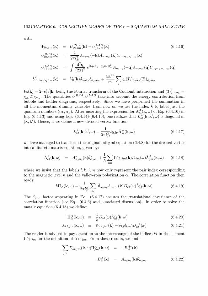
162CHAPTER 6. COLLECTIVE MODES OF THE ν = 0 QUANTUM HALL STATE
with
Wlk,jm(k) = URPAlk,jm(k)− ULAD
jk,lm(k) (6.4.16)
URPAlk,jm(k) =
1
2πl2BAnlnk
(−k)Anjnm(k)Uαlαk,αjαm
(k)
ULADjk,lm(k) =
∫
d2q
(2π)2ei(qxky−qykx)l
2BAnjnk
(−q)Anlnm(q)Uαjαk,αlαm
(q)
Uαlαk,αjαm(k) = V0(k)δαlαk
δαjαm+
4π~2
m
∑
i
gi(Ti)αlαk(Ti)αjαm
V0(k) = 2πe2c/|k| being the Fourier transform of the Coulomb interaction and (Ti)αlαk=
χ†αlTiχαk
. The quantities URPA, ULAD take into account the energy contribution frombubble and ladder diagrams, respectively. Since we have performed the summation inall the momentum dummy variables, from now on we use the index k to label just thequantum numbers (nk, αk). After inserting the expression for ΛA
kl(k, ω) of Eq. (6.4.10) inEq. (6.4.13) and using Eqs. (6.4.14)-(6.4.16), one realizes that LA
kl(k,k′, ω) is diagonal in
(k,k′). Hence, if we define a new dressed vertex function:
LAkl(k,k
′, ω) ≡ 1
2πl2Bδk,k′ΛA
kl(k, ω) (6.4.17)
we have managed to transform the original integral equation (6.4.8) for the dressed vertexinto a discrete matrix equation, given by:
ΛAkl(k, ω) = A∗
nknl(k)θ∗αkαl
+1
~
∑
jm
Wlk,jm(k)Djm(ω)ΛAjm(k, ω) (6.4.18)
where we insist that the labels l, k, j,m now only represent the pair index correspondingto the magnetic level n and the valley-spin polarization α. The correlation function thenreads:
~ΠA(k, ω) =1
2πl2B
∑
kl
θαkαlAnknl
(k)Dkl(ω)ΛAkl(k, ω) (6.4.19)
The δk,k′ factor appearing in Eq. (6.4.17) ensures the translational invariance of thecorrelation function [see Eq. (6.4.6) and associated discussion]. In order to solve thematrix equation (6.4.18) we define:
ΠAkl(k, ω) ≡ 1
~Dkl(ω)Λ
Akl(k, ω) (6.4.20)
Xkl,jm(k, ω) ≡ Wlk,jm(k) − δkjδlm~D−1kl (ω) (6.4.21)
The reader is advised to pay attention to the interchange of the indices kl in the elementWlk,jm for the definition of Xkl,jm. From these results, we find:
∑
jm
Xkl,jm(k, ω)ΠAjm(k, ω) = −BA∗
kl (k)
BAkl(k) = Anknl
(k)θαkαl(6.4.22)

6.4. COLLECTIVE MODES 163
The matrix Xkl,jm is referred as dispersion matrix in Ref. [127]. The dispersion relationof the collective modes is computed from the equation
det [X(k, ω)] = 0 (6.4.23)
as Eq. (6.4.19) can be rewritten as:
ΠA(k, ω) = − 1
2πl2B
∑
kljm
BAkl(k)X
−1kl,jmB
A∗jm(k) (6.4.24)
We clearly see from this relation that the poles of the correlation function, which give thecollective-mode energies, are given by the values at which the matrix Xkl,jm is singular.The matrices Xkl,jm(k, ω),Wlk,jm(k) present the following useful properties:
Wlk,jm(k, ω) = W ∗mj,kl(k) (6.4.25)
Xkl,jm(k, ω) = X∗lk,mj(−k,−ω∗) (6.4.26)
According to Eqs. (6.4.9),(6.4.20) and (6.4.21), the only valid matrix elements ofXkl,jm(k, ω)are those where the index pair kl correspond to one level occupied and the other levelempty (the same goes for jm). The occupation number only depend on the valley-spinindex, νk = ναk
, as argued in Section 6.3.2, and then the level unoccupied has necessar-ily different valley-spin polarization from the occupied level. This fact implies that forθA = 1, i.e., the case where ΠA is the density-density correlation function, ΠA(k, ω) = 0.This is just an artifact of our model, as we restrict ourselves to the ZLL. When we allow ar-bitrary transitions between LLs a non-vanishing density correlation function is recovered(see Sec. 6.6).
6.4.2 Dispersion relation
Preliminary remarks
In this subsection, we compute the collective mode energies using the results derived inSec. 6.4.1. As a first step, we calculate D−1
kl (ω) from Eq. (6.4.9):
D−1kl (ω) =
ω − (ωl − ωk)
νk − νl(6.4.27)
We remark that we follow the notation introduced after Eq. (6.4.16) and k labels at thesame time the magnetic index and valley-spin polarization, (nk, αk). Thus, each indexk, l takes 8 values, corresponding to the dimension of the space composed of the magneticlevels and the valley-spin subspace, |01〉⊗KK ′⊗s. As mentioned in the discussion at theend of Sec. 6.4.1, the occupation numbers of the pair kl must correspond to one filled leveland one empty level, so we have νk − νl = ±1. We remind that the occupation numbersonly depend on the valley-spin component αk and αl. Specifically, if we denote the indexpair kl as normal (anomalous) when ναk
− ναl= 1 (ναk
− ναl= −1), we have that kl is
normal for αkαl = ac, ad, bc, bd and anomalous when αkαl = ca, da, cb, db. Therefore, thecollective modes here computed correspond to intra-LL valley-spin waves [110]. A direct

164CHAPTER 6. COLLECTIVE MODES OF THE ν = 0 QUANTUM HALL STATE
consequence of this fact is that the Coulomb contribution to the RPA energy, URPA,vanishes; see Eq. (6.4.16). In respect to the orbital structure of the collective modes, it iswell known that they are described in terms of the so-called magnetoexciton wave-function[126].
The considerations of the previous paragraph induce a very special structure in the to-tal matrix Xkl,jm(k, ω), which can be expressed using the 4×4 matrices Y αkαl,αjαm(k, ω)as building blocks. These matrices result from considering all the possible values in themagnetic level subspace, nknl = 00, 01, 10, 11, for a fixed set of values of the valley-spincomponents (αkαl, αjαm), i.e.
Y αkαl,αjαm(k, ω) = (6.4.28)
=
Yαkαl,αjαm
00,00 (k, ω) Yαkαl,αjαm
00,01 (k, ω) Yαkαl,αjαm
00,10 (k, ω) Yαkαl,αjαm
00,11 (k, ω)Y
αkαl,αjαm
01,00 (k, ω) Yαkαl,αjαm
01,01 (k, ω) Yαkαl,αjαm
01,10 (k, ω) Yαkαl,αjαm
01,11 (k, ω)
Yαkαl,αjαm
10,00 (k, ω) Yαkαl,αjαm
10,01 (k, ω) Yαkαl,αjαm
10,10 (k, ω) Yαkαl,αjαm
10,11 (k, ω)Y
αkαl,αjαm
11,00 (k, ω) Yαkαl,αjαm
11,01 (k, ω) Yαkαl,αjαm
11,10 (k, ω) Yαkαl,αjαm
11,11 (k, ω)
with
Y αkαl,αjαmnknl,njnm
(k, ω) ≡ Xkl,jm(k, ω) (6.4.29)
The explicit form of Y αkαl,αjαm(k, ω) is computed from Eqs. (6.4.16), (6.4.21) andreads:
Y αkαl,αjαm(k, ω) = [(ναk− ναl
)(Eαkαl − ~ωI)− C(k)]δαkαjδαlαm
+R(k)Mαkαl,αjαm
Mαkαl,αjαm ≡∑
i
ui[(Ti)αlαk(Ti)αjαm
− (Ti)αjαk(Ti)αlαm
] , (6.4.30)
I being the identity 4 × 4 matrix. The matrix C takes into account the (ladder) con-tribution from the Coulomb interaction while short-range interactions give rise to the Rmatrix, which is the same for both ladder and bubble contributions. The expressions forthese matrices are given in Appendix K. The matrix Eαkαl is diagonal and arises fromthe term D−1
kl (ω); its elements are given by Eαkαlnknl,njnm
= (ǫnl,αl− ǫnk,αk
)δnknjδnlnm
.
On the other hand, as explained before, we only have to take into account indicesαkαl in such way that they correspond to one filled and one empty level. A simple countthen reveals that the total matrix Xkl,jm(k, ω) is 32× 32. We also see from Eq. (6.4.30)that the matrix Y αkαl,αjαm(k, ω) can be separated as
Y αkαl,αjαm(k, ω) = Y αkαl,αjαm(k)−(ναk−ναl
)~ωI, Y αkαl,αjαm(k) ≡ Y αkαl,αjαm(k, ω = 0)(6.4.31)
This relation tells us that Eq. (6.4.23) is a generalized eigenvalue equation that reduces tothe usual eigenvalue equation for ω (−ω) for normal (anomalous) indices [this fact is at theorigin of the symmetry (6.4.26)]. The conclusion reached is that the computation of thecollective-mode frequencies amounts to the obtention of the eigenvalues of the following

6.4. COLLECTIVE MODES 165
32× 32 matrix:
Xkl,jm(k) ≡ σzXkl,jm(k, 0) (6.4.32)
=
Y ac,ac Y ac,ad Y ac,bc Y ac,bd Y ac,ca Y ac,da Y ac,cb Y ac,db
Y ad,ac Y ad,ad Y ad,bc Y ad,bd Y ad,ca Y ad,da Y ad,cb Y ad,db
Y bc,ac Y bc,ad Y bc,bc Y bc,bd Y bc,ca Y bc,da Y bc,cb Y bc,db
Y bd,ac Y bd,ad Y bd,bc Y bd,bd Y bd,ca Y bd,da Y bd,cb Y bd,db
−Y ca,ac −Y ca,ad −Y ca,bc −Y ca,bd −Y ca,ca −Y ca,da −Y ca,cb −Y ca,db
−Y da,ac −Y da,ad −Y da,bc −Y da,bd −Y da,ca −Y da,da −Y da,cb −Y da,db
−Y cb,ac −Y cb,ad −Y cb,bc −Y cb,bd −Y cb,ca −Y cb,da −Y cb,cb −Y cb,db
−Y db,ac −Y db,ad −Y db,bc −Y db,bd −Y db,ca −Y db,da −Y db,cb −Y db,db
with σz a 32 × 32 diagonal matrix of the form σz = diag[I, I, I, I,−I,−I,−I,−I]. Thehorizontal and vertical lines in Eq. (6.4.32) separate the normal and anomalous sectors,yielding an analog structure to that of the bosonic BdG equations discussed along thefirst chapters. Indeed, the BdG equations can be regarded as generalized RPA equations[128].
Because the term between square brackets in Eq. (6.4.30) (which contains the electron-hole energy difference and the Coulomb interaction contributions) is multiplied by a di-agonal tensor with respect to the valley-spin indices, the different valley-spin sectors of Xare only connected through the term arising from short-range interactions Mαkαl,αjαm ,that is, for αkαl 6= αjαm
Y αkαl,αjαm(k, 0) = R(k)Mαkαl,αjαm (6.4.33)
The coefficients Mαkαl,αjαm , given in Eq. (6.4.30), present the following symmetries
Mαkαl,αjαm = (Mαjαm,αkαl)∗ = (Mαlαk,αmαj )∗ = −Mαkαj ,αlαm (6.4.34)
The point of writing the matrix X in this form is that the previous properties simplifynotably the calculations since, in practice, many of the coefficients Mαkαl,αjαm vanishand consequently we do not need to take into account the full 32× 32 matrix in order tocompute the collective modes. In particular, whenever Mαkαl,αjαm does not mix normaland anomalous sectors of the matrix Xkl,jm [i.e., the off-diagonal boxes in Eq. (6.4.32)vanish], the computation of the dispersion relation is reduced to the computation of theeigenvalues of ±Xkl,jm(k, 0) evaluated in the normal (anomalous) sector. If this is thecase, the property (6.4.25) automatically guarantees that ω is real. In Appendix K, weshow that the dispersion relation is isotropic and hence only depends on k = |k| (not tobe confused with the index k in the matrix elements).
Interestingly, at k = 0, the dispersion relation can be obtained analytically aftermaking a symmetric and antisymmetric combination of the magnetic indices of the form
S,A =00± 11√
2, (6.4.35)
that yields a simplified matrix
Y αkαl,αjαm(k = 0) = (F +∆αkαlI) δαkαjδαlαm
+QMαkαl,αjαm (6.4.36)
F = diag[0,F00 + F11
2,F00 + F11
2, 2F01], Q = diag[1, 0, 0, 0]

166CHAPTER 6. COLLECTIVE MODES OF THE ν = 0 QUANTUM HALL STATE
where the order of the magnetic indices for rows and columns is now S, 01, 10, A. Thequantity ∆αkαl = |ǫαl
− ǫαk| is the energy difference related only to the valley-spin part
[see Eq. (6.3.8)]. Thus, all matrices in Eq. (6.4.36) are already diagonal in the magneticsubspace. In particular, the only magnetic matrix element which is connected to othervalley-spin sectors is that associated to the symmetric combination S of Eq. (6.4.35).For the other magnetic matrix elements, the collective-mode frequencies are immediatelyobtained from the diagonal of F + ∆αkαlI. Hence, at k = 0, the symmetric modes Srepresent the lowest-frequency modes because they do not depend on the strength of theCoulomb interaction. We note that these modes are the same as the “even” modes of Ref.[111] and they arise due to the exact conservation of the quantum number lz ≡ |nl|− |nk|at k = 0, that corresponds to the angular momentum of the magnetoexciton at zeromomentum [110]. The prolongations for k 6= 0 of the symmetric modes frequencies,ωS(0), increase with k. Therefore, we conclude that the symmetric modes S characterizethe phase transitions as they represent the lowest energy excitations of the system and,remarkably, their calculation is always analytical. On the opposite limit, klB & 1, onlyCoulomb interactions are relevant since C(k) decays as k−1 while R(k) does it as
R(k) ∼ e−(klB )2
2 , (6.4.37)
see Appendix K for the proof. We then expect to recover in this limit the results of Refs.[111, 113] for the dispersion relation. For klB ≫ 1, the collective modes approach tothe mean-field excitations ω ≃ ωnl,αl
− ωnk,αk. For arbitrary momentum, the dispersion
relation is computed numerically.
Collective modes: numerical and analytical results
In this section, we obtain the dispersion relation for the different ground states obtainedin Sec. 6.3.2, in which the occupied (unoccupied) valley-spin polarizations were labeledas a, b (c, d), see Eqs. (6.3.10),(6.3.11),(6.3.13),(6.3.15) to check the mean-field solutionsand the notation. For all the phases, we give the values of the valley-spin energies ∆αkαl
and of the independent non-vanishing coefficientsMαkαl,αjαm and obtain analytically thesymmetric frequencies ωS(0) that represent the lowest-energy excitations. In the rest ofthis section, we only use k to denote the norm of the wave vector, k = |k|.
Ferromagnetic phase:
∆ac = ∆bd = 2ǫZ + 2u⊥ + uz, ∆ad,bc = ∆ac ± 2ǫV (6.4.38)
Mac,ac = M bd,bd = −uz, Mac,bd = −2u⊥, Mbc,bc =Mad,ad = uz
As the unoccupied levels have orthogonal spin polarizations to the occupied levels, thereis no mixing between normal and anomalous indices and the RPA contribution vanishes.The computation of the collective modes frequency then reduces to solve an eigenvalueequation that gives always real frequencies, see discussion below Eq. (6.4.33). Conse-quently, we focus on computing the dispersion relation ω(k) on the normal sector, andthe dispersion relation in the anomalous sector is just −ω(k).
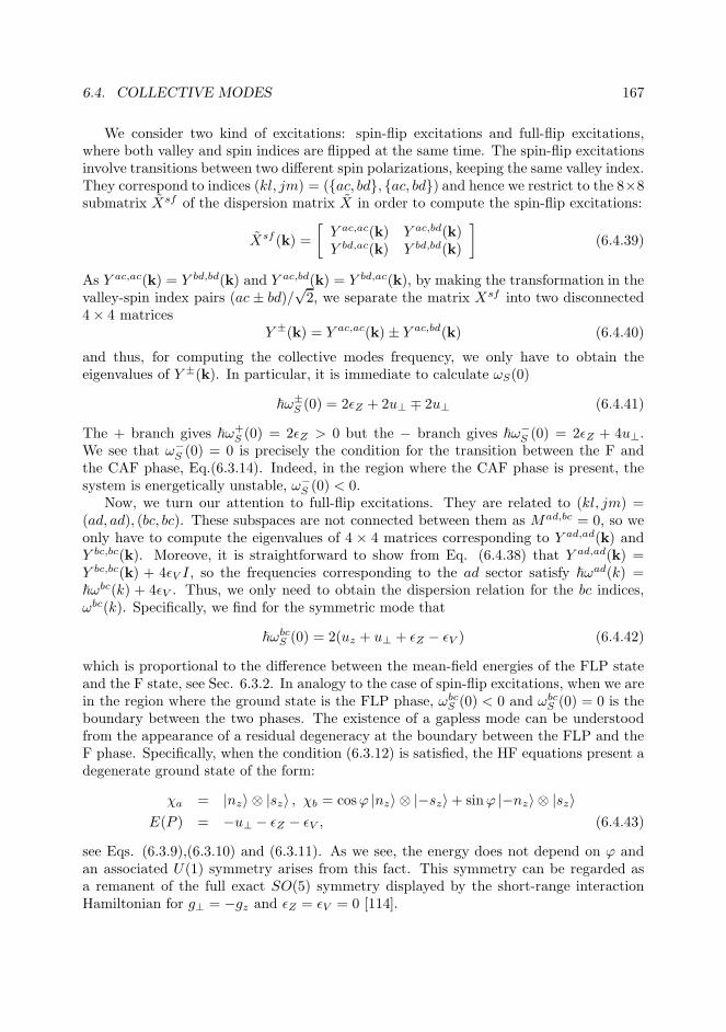
6.4. COLLECTIVE MODES 167
We consider two kind of excitations: spin-flip excitations and full-flip excitations,where both valley and spin indices are flipped at the same time. The spin-flip excitationsinvolve transitions between two different spin polarizations, keeping the same valley index.They correspond to indices (kl, jm) = (ac, bd, ac, bd) and hence we restrict to the 8×8submatrix Xsf of the dispersion matrix X in order to compute the spin-flip excitations:
Xsf (k) =
[
Y ac,ac(k) Y ac,bd(k)Y bd,ac(k) Y bd,bd(k)
]
(6.4.39)
As Y ac,ac(k) = Y bd,bd(k) and Y ac,bd(k) = Y bd,ac(k), by making the transformation in thevalley-spin index pairs (ac ± bd)/
√2, we separate the matrix Xsf into two disconnected
4× 4 matricesY ±(k) = Y ac,ac(k) ± Y ac,bd(k) (6.4.40)
and thus, for computing the collective modes frequency, we only have to obtain theeigenvalues of Y ±(k). In particular, it is immediate to calculate ωS(0)
~ω±S (0) = 2ǫZ + 2u⊥ ∓ 2u⊥ (6.4.41)
The + branch gives ~ω+S (0) = 2ǫZ > 0 but the − branch gives ~ω−
S (0) = 2ǫZ + 4u⊥.We see that ω−
S (0) = 0 is precisely the condition for the transition between the F andthe CAF phase, Eq.(6.3.14). Indeed, in the region where the CAF phase is present, thesystem is energetically unstable, ω−
S (0) < 0.Now, we turn our attention to full-flip excitations. They are related to (kl, jm) =
(ad, ad), (bc, bc). These subspaces are not connected between them as Mad,bc = 0, so weonly have to compute the eigenvalues of 4 × 4 matrices corresponding to Y ad,ad(k) andY bc,bc(k). Moreove, it is straightforward to show from Eq. (6.4.38) that Y ad,ad(k) =Y bc,bc(k) + 4ǫV I, so the frequencies corresponding to the ad sector satisfy ~ωad(k) =~ωbc(k) + 4ǫV . Thus, we only need to obtain the dispersion relation for the bc indices,ωbc(k). Specifically, we find for the symmetric mode that
~ωbcS (0) = 2(uz + u⊥ + ǫZ − ǫV ) (6.4.42)
which is proportional to the difference between the mean-field energies of the FLP stateand the F state, see Sec. 6.3.2. In analogy to the case of spin-flip excitations, when we arein the region where the ground state is the FLP phase, ωbc
S (0) < 0 and ωbcS (0) = 0 is the
boundary between the two phases. The existence of a gapless mode can be understoodfrom the appearance of a residual degeneracy at the boundary between the FLP and theF phase. Specifically, when the condition (6.3.12) is satisfied, the HF equations present adegenerate ground state of the form:
χa = |nz〉 ⊗ |sz〉 , χb = cosϕ |nz〉 ⊗ |−sz〉+ sinϕ |−nz〉 ⊗ |sz〉E(P ) = −u⊥ − ǫZ − ǫV , (6.4.43)
see Eqs. (6.3.9),(6.3.10) and (6.3.11). As we see, the energy does not depend on ϕ andan associated U(1) symmetry arises from this fact. This symmetry can be regarded asa remanent of the full exact SO(5) symmetry displayed by the short-range interactionHamiltonian for g⊥ = −gz and ǫZ = ǫV = 0 [114].
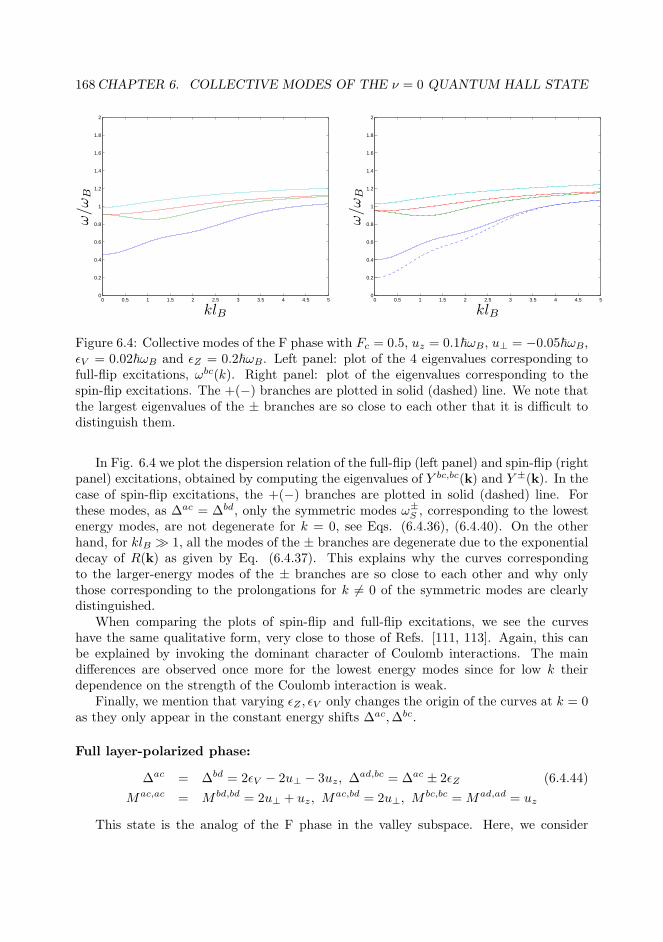
168CHAPTER 6. COLLECTIVE MODES OF THE ν = 0 QUANTUM HALL STATE
0 0.5 1 1.5 2 2.5 3 3.5 4 4.5 50
0.2
0.4
0.6
0.8
1
1.2
1.4
1.6
1.8
2
klB
ω/ω
B
0 0.5 1 1.5 2 2.5 3 3.5 4 4.5 50
0.2
0.4
0.6
0.8
1
1.2
1.4
1.6
1.8
2
klB
ω/ω
B
Figure 6.4: Collective modes of the F phase with Fc = 0.5, uz = 0.1~ωB, u⊥ = −0.05~ωB,ǫV = 0.02~ωB and ǫZ = 0.2~ωB. Left panel: plot of the 4 eigenvalues corresponding tofull-flip excitations, ωbc(k). Right panel: plot of the eigenvalues corresponding to thespin-flip excitations. The +(−) branches are plotted in solid (dashed) line. We note thatthe largest eigenvalues of the ± branches are so close to each other that it is difficult todistinguish them.
In Fig. 6.4 we plot the dispersion relation of the full-flip (left panel) and spin-flip (rightpanel) excitations, obtained by computing the eigenvalues of Y bc,bc(k) and Y ±(k). In thecase of spin-flip excitations, the +(−) branches are plotted in solid (dashed) line. Forthese modes, as ∆ac = ∆bd, only the symmetric modes ω±
S , corresponding to the lowestenergy modes, are not degenerate for k = 0, see Eqs. (6.4.36), (6.4.40). On the otherhand, for klB ≫ 1, all the modes of the ± branches are degenerate due to the exponentialdecay of R(k) as given by Eq. (6.4.37). This explains why the curves correspondingto the larger-energy modes of the ± branches are so close to each other and why onlythose corresponding to the prolongations for k 6= 0 of the symmetric modes are clearlydistinguished.
When comparing the plots of spin-flip and full-flip excitations, we see the curveshave the same qualitative form, very close to those of Refs. [111, 113]. Again, this canbe explained by invoking the dominant character of Coulomb interactions. The maindifferences are observed once more for the lowest energy modes since for low k theirdependence on the strength of the Coulomb interaction is weak.
Finally, we mention that varying ǫZ , ǫV only changes the origin of the curves at k = 0as they only appear in the constant energy shifts ∆ac,∆bc.
Full layer-polarized phase:
∆ac = ∆bd = 2ǫV − 2u⊥ − 3uz, ∆ad,bc = ∆ac ± 2ǫZ (6.4.44)
Mac,ac = M bd,bd = 2u⊥ + uz, Mac,bd = 2u⊥, M
bc,bc =Mad,ad = uz
This state is the analog of the F phase in the valley subspace. Here, we consider

6.4. COLLECTIVE MODES 169
valley-flip excitations and full-flip excitations. Again, it can be shown that there is nomixing between normal and anomalous sectors, so the computation can be carried out ina similar fashion to the F state. The computation for the valley-flip excitations is formallyequal to the F case, see Eq. (6.4.40) and related discussion. However, a peculiarity arisesfor the FLP phase. It can be shown that ~ω−(k) = ~ωbc(k) + 2ǫZ, where ω
bc(k) is thefrequency corresponding to the full-flip excitations, as explained later. Thus, half of themodes corresponding to valley-flip excitations are indeed full-flip excitations. The originof this fact can be trace back to the spin invariance of the interaction. As a consequence,we only need to compute ω+(k) for characterizing the valley-flip excitations. At k = 0,the symmetric mode is given by:
~ω+S (0) = 2u⊥ − 2uz + 2ǫV (6.4.45)
In analogy to the case of the F-CAF transition [see Eq. (6.4.41) and related discussion],ω+S (0) becomes negative in the region where the PLP phase is present. Precisely, ω+
S (0) =0 is the boundary between the two phases. Thus, the FLP state becomes energeticallyunstable in the region where the PLP phase is present, as expected.
On the other hand, as for the F phase, the full-flip excitations describe the transitionbetween the F and FLP phase. The calculation is formally analog to that of the F phaseand we also find a similar relation, ~ωad(k) = ~ωbc(k) + 4ǫV . For studying the phasetransition, we obtain the symmetric mode
~ωbcS (0) = 2(ǫV − ǫZ − u⊥ − uz) (6.4.46)
which is just −ωbcS (0) for the F state, see Eq. (6.4.42). Reasoning as before, the FLP
phase becomes unstable in the region where the F phase is present and the appearanceof the zero-frequency mode at the boundary between the two regions results from theaccidental U(1) symmetry, see Eqs. (6.4.42),(6.4.43).
In Fig. 6.5, we represent the dispersion relation of the full-flip (left panel) and propervalley-flip (right panel) excitations. The qualitative trends and properties of the curvesare similar to those of the F state.
Canted anti-ferromagnetic phase:
∆ac = ∆bd = uz − 2u⊥, ∆ad,bc = ∆ac ± 2ǫV (6.4.47)
Mac,ac = M bd,bd = −uz, Mac,bd = −2u⊥ cos2 θs
M bc,bc = Mad,ad = uz + 2u⊥ sin2 θs, Mac,db = −2u⊥ sin2 θs
In this case, the coefficientsMαkαl,αjαm mix normal and anomalous indices. In particular,for studying the equivalent of the spin-flip modes, we have to compute the eigenvalues ofthe 16× 16 matrix Xsf(k):
Xsf (k) =
Y ac,ac(k) Y ac,bd(k) 0 Y ac,db(k)Y bd,ac(k) Y bd,bd(k) Y bd,ca(k) 0
0 −Y ca,bd(k) −Y ca,ca(k) −Y ca,db(k)−Y db,ac(k) 0 −Y db,ca(k) −Y db,db(k)
(6.4.48)
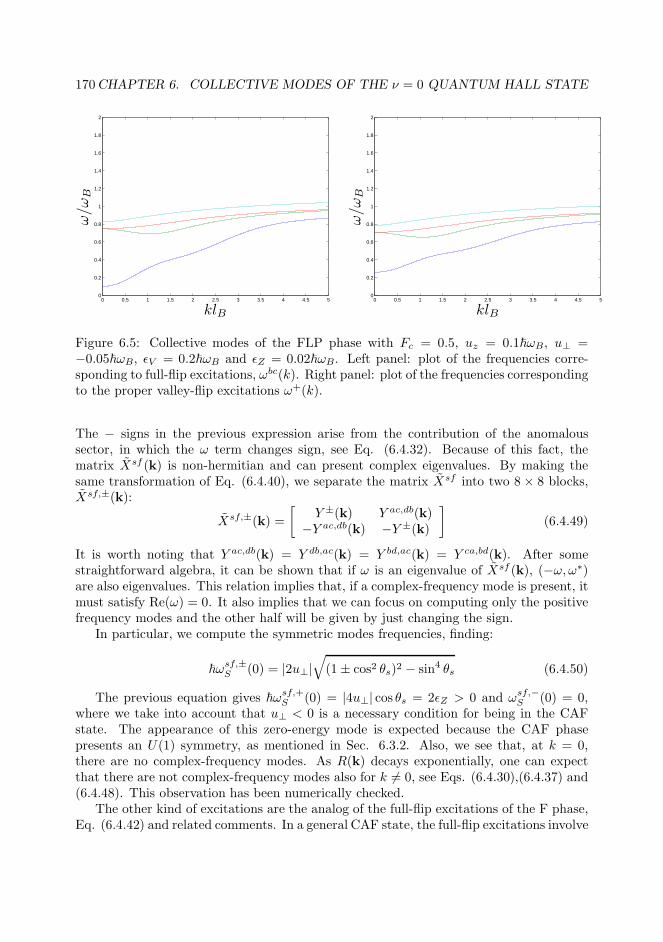
170CHAPTER 6. COLLECTIVE MODES OF THE ν = 0 QUANTUM HALL STATE
0 0.5 1 1.5 2 2.5 3 3.5 4 4.5 50
0.2
0.4
0.6
0.8
1
1.2
1.4
1.6
1.8
2
klB
ω/ω
B
0 0.5 1 1.5 2 2.5 3 3.5 4 4.5 50
0.2
0.4
0.6
0.8
1
1.2
1.4
1.6
1.8
2
klB
ω/ω
B
Figure 6.5: Collective modes of the FLP phase with Fc = 0.5, uz = 0.1~ωB, u⊥ =−0.05~ωB, ǫV = 0.2~ωB and ǫZ = 0.02~ωB. Left panel: plot of the frequencies corre-sponding to full-flip excitations, ωbc(k). Right panel: plot of the frequencies correspondingto the proper valley-flip excitations ω+(k).
The − signs in the previous expression arise from the contribution of the anomaloussector, in which the ω term changes sign, see Eq. (6.4.32). Because of this fact, thematrix Xsf (k) is non-hermitian and can present complex eigenvalues. By making thesame transformation of Eq. (6.4.40), we separate the matrix Xsf into two 8 × 8 blocks,Xsf,±(k):
Xsf,±(k) =
[
Y ±(k) Y ac,db(k)−Y ac,db(k) −Y ±(k)
]
(6.4.49)
It is worth noting that Y ac,db(k) = Y db,ac(k) = Y bd,ac(k) = Y ca,bd(k). After somestraightforward algebra, it can be shown that if ω is an eigenvalue of Xsf (k), (−ω, ω∗)are also eigenvalues. This relation implies that, if a complex-frequency mode is present, itmust satisfy Re(ω) = 0. It also implies that we can focus on computing only the positivefrequency modes and the other half will be given by just changing the sign.
In particular, we compute the symmetric modes frequencies, finding:
~ωsf,±S (0) = |2u⊥|
√
(1± cos2 θs)2 − sin4 θs (6.4.50)
The previous equation gives ~ωsf,+S (0) = |4u⊥| cos θs = 2ǫZ > 0 and ωsf,−
S (0) = 0,where we take into account that u⊥ < 0 is a necessary condition for being in the CAFstate. The appearance of this zero-energy mode is expected because the CAF phasepresents an U(1) symmetry, as mentioned in Sec. 6.3.2. Also, we see that, at k = 0,there are no complex-frequency modes. As R(k) decays exponentially, one can expectthat there are not complex-frequency modes also for k 6= 0, see Eqs. (6.4.30),(6.4.37) and(6.4.48). This observation has been numerically checked.
The other kind of excitations are the analog of the full-flip excitations of the F phase,Eq. (6.4.42) and related comments. In a general CAF state, the full-flip excitations involve
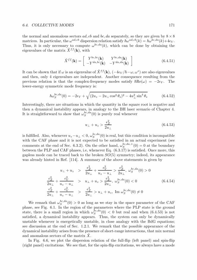
6.4. COLLECTIVE MODES 171
the normal and anomalous sectors ad, cb and bc, da separately, so they are given by 8× 8matrices. In particular, the ωad,cb dispersion relation satisfy ~ωad,cb(k) = ~ωbc,da(k)+4ǫV .Thus, it is only necessary to compute ωbc,da(k), which can be done by obtaining theeigenvalues of the matrix Xff (k), with
Xff(k) =
[
Y bc,bc(k) Y bc,da(k)−Y da,bc(k) −Y da,da(k)
]
(6.4.51)
It can be shown that if ω is an eigenvalue of Xff(k), (−4ǫV /~−ω, ω∗) are also eigenvaluesand then, only 4 eigenvalues are independent. Another consequence resulting from theprevious relation is that the complex-frequency modes satisfy ~Re(ω) = −2ǫV . Thelower-energy symmetric mode frequency is:
~ωbc,daS (0) = −2ǫV +
√
(2uz − 2u⊥ cos2 θs)2 − 4u2⊥ sin4 θs (6.4.52)
Interestingly, there are situations in which the quantity in the square root is negative andthen a dynamical instability appears, in analogy to the BH laser scenario of Chapter 4.It is straightforward to show that ωbc,da
S (0) is purely real whenever
u⊥ + uz >ǫ2Z2u⊥
(6.4.53)
is fulfilled. Also, whenever uz−u⊥ < 0, ωbc,daS (0) is real, but this condition is incompatible
with the CAF phase and it is not expected to be satisfied in an actual experiment (see
comments at the end of Sec. 6.3.2). On the other hand, ωbc,da,+S (0) = 0 at the boundary
between the PLP and CAF phases, i.e, whenever Eq. (6.3.17) is satisfied. Once more, thisgapless mode can be traced back to the broken SO(5) symmetry; indeed, its appearancewas already hinted in Ref. [114]. A summary of the above statements is given by
u⊥ + uz >ǫ2Z2u⊥
+ǫ2V
uz − u⊥>
ǫ2Z2u⊥
, ωbc,daS (0) > 0
ǫ2Z2u⊥
+ǫ2V
uz − u⊥> u⊥ + uz >
ǫ2Z2u⊥
, ωbc,daS (0) < 0 (6.4.54)
ǫ2Z2u⊥
+ǫ2V
uz − u⊥>
ǫ2Z2u⊥
> u⊥ + uz, Im ωbc,daS (0) 6= 0
We remark that ωbc,daS (0) > 0 as long as we stay in the space parameter of the CAF
phase, see Fig. 6.1. In the region of the parameters where the PLP state is the groundstate, there is a small region in which ωbc,da
S (0) < 0 but real and when (6.4.53) is notsatisfied, a dynamical instability appears. Thus, the system can only be dynamicallyunstable whenever is energetically unstable, in close analogy with the BdG equations;see discussion at the end of Sec. 1.2.1. We remark that the possible appearance of thedynamical instability arises from the presence of short-range interactions, that mix normaland anomalous sectors of the matrix X.
In Fig. 6.6, we plot the dispersion relation of the full-flip (left panel) and spin-flip(right panel) excitations. We see that, for the spin-flip excitations, we always have a mode
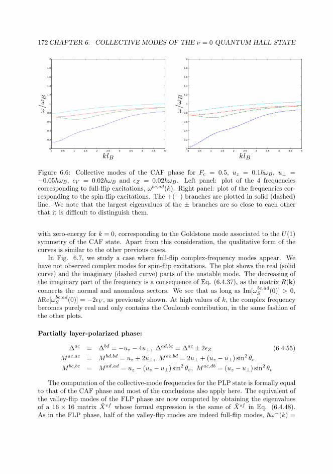
172CHAPTER 6. COLLECTIVE MODES OF THE ν = 0 QUANTUM HALL STATE
0 0.5 1 1.5 2 2.5 3 3.5 4 4.5 50
0.2
0.4
0.6
0.8
1
1.2
1.4
1.6
1.8
2
klB
ω/ω
B
0 0.5 1 1.5 2 2.5 3 3.5 4 4.5 50
0.2
0.4
0.6
0.8
1
1.2
1.4
1.6
1.8
2
klB
ω/ω
B
Figure 6.6: Collective modes of the CAF phase for Fc = 0.5, uz = 0.1~ωB, u⊥ =−0.05~ωB, ǫV = 0.02~ωB and ǫZ = 0.02~ωB. Left panel: plot of the 4 frequenciescorresponding to full-flip excitations, ωbc,ad(k). Right panel: plot of the frequencies cor-responding to the spin-flip excitations. The +(−) branches are plotted in solid (dashed)line. We note that the largest eigenvalues of the ± branches are so close to each otherthat it is difficult to distinguish them.
with zero-energy for k = 0, corresponding to the Goldstone mode associated to the U(1)symmetry of the CAF state. Apart from this consideration, the qualitative form of thecurves is similar to the other previous cases.
In Fig. 6.7, we study a case where full-flip complex-frequency modes appear. Wehave not observed complex modes for spin-flip excitations. The plot shows the real (solidcurve) and the imaginary (dashed curve) parts of the unstable mode. The decreasing ofthe imaginary part of the frequency is a consequence of Eq. (6.4.37), as the matrix R(k)
connects the normal and anomalous sectors. We see that as long as Im[ωbc,adS (0)] > 0,
~Re[ωbc,adS (0)] = −2ǫV , as previously shown. At high values of k, the complex frequency
becomes purely real and only contains the Coulomb contribution, in the same fashion ofthe other plots.
Partially layer-polarized phase:
∆ac = ∆bd = −uz − 4u⊥, ∆ad,bc = ∆ac ± 2ǫZ (6.4.55)
Mac,ac = M bd,bd = uz + 2u⊥, Mac,bd = 2u⊥ + (uz − u⊥) sin
2 θv
M bc,bc = Mad,ad = uz − (uz − u⊥) sin2 θv, M
ac,db = (uz − u⊥) sin2 θv
The computation of the collective-mode frequencies for the PLP state is formally equalto that of the CAF phase and most of the conclusions also apply here. The equivalent ofthe valley-flip modes of the FLP phase are now computed by obtaining the eigenvaluesof a 16 × 16 matrix Xvf whose formal expression is the same of Xsf in Eq. (6.4.48).As in the FLP phase, half of the valley-flip modes are indeed full-flip modes, ~ω−(k) =
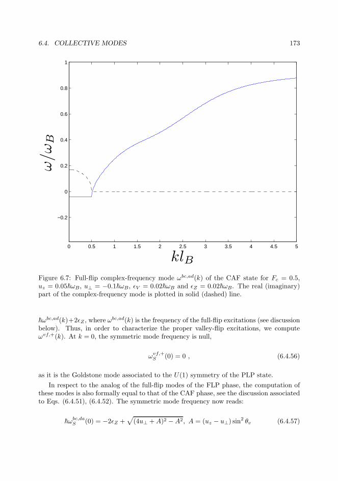
6.4. COLLECTIVE MODES 173
0 0.5 1 1.5 2 2.5 3 3.5 4 4.5 5
−0.2
0
0.2
0.4
0.6
0.8
1
klB
ω/ω
B
Figure 6.7: Full-flip complex-frequency mode ωbc,ad(k) of the CAF state for Fc = 0.5,uz = 0.05~ωB, u⊥ = −0.1~ωB, ǫV = 0.02~ωB and ǫZ = 0.02~ωB. The real (imaginary)part of the complex-frequency mode is plotted in solid (dashed) line.
~ωbc,ad(k)+2ǫZ , where ωbc,ad(k) is the frequency of the full-flip excitations (see discussion
below). Thus, in order to characterize the proper valley-flip excitations, we computeωvf,+(k). At k = 0, the symmetric mode frequency is null,
ωvf,+S (0) = 0 , (6.4.56)
as it is the Goldstone mode associated to the U(1) symmetry of the PLP state.
In respect to the analog of the full-flip modes of the FLP phase, the computation ofthese modes is also formally equal to that of the CAF phase, see the discussion associatedto Eqs. (6.4.51), (6.4.52). The symmetric mode frequency now reads:
~ωbc,daS (0) = −2ǫZ +
√
(4u⊥ +A)2 −A2, A = (uz − u⊥) sin2 θv (6.4.57)
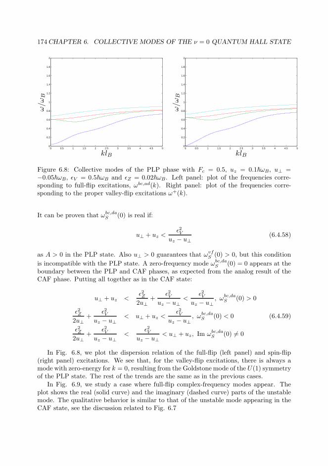
174CHAPTER 6. COLLECTIVE MODES OF THE ν = 0 QUANTUM HALL STATE
0 0.5 1 1.5 2 2.5 3 3.5 4 4.5 50
0.2
0.4
0.6
0.8
1
1.2
1.4
1.6
1.8
2
klB
ω/ω
B
0 0.5 1 1.5 2 2.5 3 3.5 4 4.5 50
0.2
0.4
0.6
0.8
1
1.2
1.4
1.6
1.8
2
klB
ω/ω
B
Figure 6.8: Collective modes of the PLP phase with Fc = 0.5, uz = 0.1~ωB, u⊥ =−0.05~ωB, ǫV = 0.5~ωB and ǫZ = 0.02~ωB. Left panel: plot of the frequencies corre-sponding to full-flip excitations, ωbc,ad(k). Right panel: plot of the frequencies corre-sponding to the proper valley-flip excitations ω+(k).
It can be proven that ωbc,daS (0) is real if:
u⊥ + uz <ǫ2V
uz − u⊥(6.4.58)
as A > 0 in the PLP state. Also u⊥ > 0 guarantees that ωvfS (0) > 0, but this condition
is incompatible with the PLP state. A zero-frequency mode ωbc,daS (0) = 0 appears at the
boundary between the PLP and CAF phases, as expected from the analog result of theCAF phase. Putting all together as in the CAF state:
u⊥ + uz <ǫ2Z2u⊥
+ǫ2V
uz − u⊥<
ǫ2Vuz − u⊥
, ωbc,daS (0) > 0
ǫ2Z2u⊥
+ǫ2V
uz − u⊥< u⊥ + uz <
ǫ2Vuz − u⊥
, ωbc,daS (0) < 0 (6.4.59)
ǫ2Z2u⊥
+ǫ2V
uz − u⊥<
ǫ2Vuz − u⊥
< u⊥ + uz, Im ωbc,daS (0) 6= 0
In Fig. 6.8, we plot the dispersion relation of the full-flip (left panel) and spin-flip(right panel) excitations. We see that, for the valley-flip excitations, there is always amode with zero-energy for k = 0, resulting from the Goldstone mode of the U(1) symmetryof the PLP state. The rest of the trends are the same as in the previous cases.
In Fig. 6.9, we study a case where full-flip complex-frequency modes appear. Theplot shows the real (solid curve) and the imaginary (dashed curve) parts of the unstablemode. The qualitative behavior is similar to that of the unstable mode appearing in theCAF state, see the discussion related to Fig. 6.7
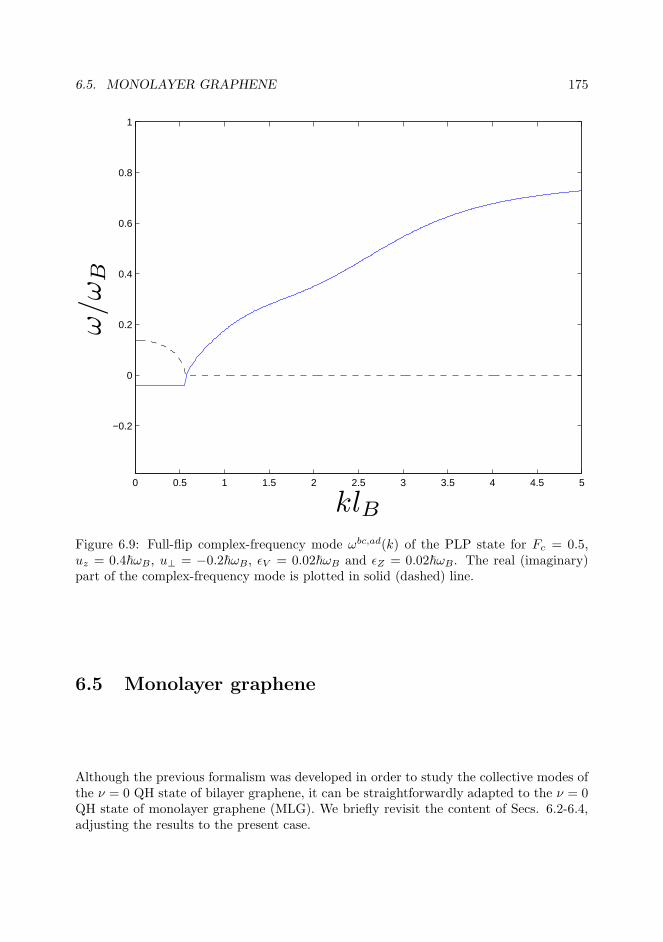
6.5. MONOLAYER GRAPHENE 175
0 0.5 1 1.5 2 2.5 3 3.5 4 4.5 5
−0.2
0
0.2
0.4
0.6
0.8
1
klB
ω/ω
B
Figure 6.9: Full-flip complex-frequency mode ωbc,ad(k) of the PLP state for Fc = 0.5,uz = 0.4~ωB, u⊥ = −0.2~ωB, ǫV = 0.02~ωB and ǫZ = 0.02~ωB. The real (imaginary)part of the complex-frequency mode is plotted in solid (dashed) line.
6.5 Monolayer graphene
Although the previous formalism was developed in order to study the collective modes ofthe ν = 0 QH state of bilayer graphene, it can be straightforwardly adapted to the ν = 0QH state of monolayer graphene (MLG). We briefly revisit the content of Secs. 6.2-6.4,adjusting the results to the present case.
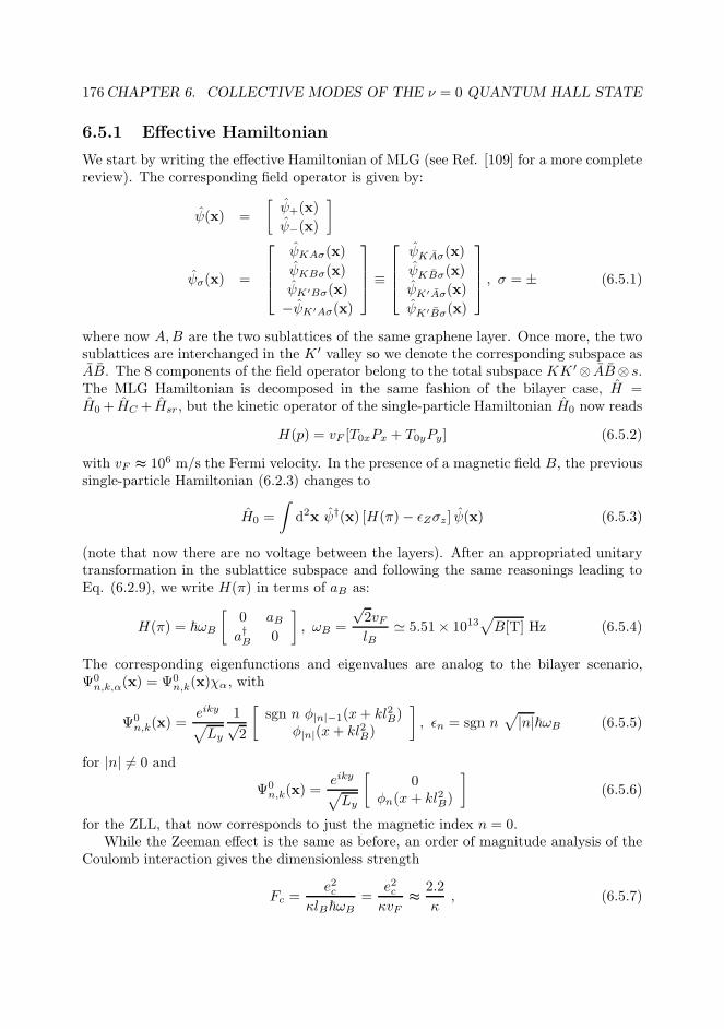
176CHAPTER 6. COLLECTIVE MODES OF THE ν = 0 QUANTUM HALL STATE
6.5.1 Effective Hamiltonian
We start by writing the effective Hamiltonian of MLG (see Ref. [109] for a more completereview). The corresponding field operator is given by:
ψ(x) =
[
ψ+(x)
ψ−(x)
]
ψσ(x) =
ψKAσ(x)
ψKBσ(x)
ψK′Bσ(x)
−ψK′Aσ(x)
≡
ψKAσ(x)
ψKBσ(x)
ψK′Aσ(x)
ψK′Bσ(x)
, σ = ± (6.5.1)
where now A,B are the two sublattices of the same graphene layer. Once more, the twosublattices are interchanged in the K ′ valley so we denote the corresponding subspace asAB. The 8 components of the field operator belong to the total subspace KK ′⊗ AB⊗ s.The MLG Hamiltonian is decomposed in the same fashion of the bilayer case, H =H0 + HC + Hsr, but the kinetic operator of the single-particle Hamiltonian H0 now reads
H(p) = vF [T0xPx + T0yPy] (6.5.2)
with vF ≈ 106 m/s the Fermi velocity. In the presence of a magnetic field B, the previoussingle-particle Hamiltonian (6.2.3) changes to
H0 =
∫
d2x ψ†(x) [H(π)− ǫZσz ] ψ(x) (6.5.3)
(note that now there are no voltage between the layers). After an appropriated unitarytransformation in the sublattice subspace and following the same reasonings leading toEq. (6.2.9), we write H(π) in terms of aB as:
H(π) = ~ωB
[
0 aBa†B 0
]
, ωB =
√2vFlB
≃ 5.51× 10¹³√
B[T] Hz (6.5.4)
The corresponding eigenfunctions and eigenvalues are analog to the bilayer scenario,Ψ0
n,k,α(x) = Ψ0n,k(x)χα, with
Ψ0n,k(x) =
eiky√
Ly
1√2
[
sgn n φ|n|−1(x+ kl2B)φ|n|(x+ kl2B)
]
, ǫn = sgn n√
|n|~ωB (6.5.5)
for |n| 6= 0 and
Ψ0n,k(x) =
eiky√
Ly
[
0φn(x+ kl2B)
]
(6.5.6)
for the ZLL, that now corresponds to just the magnetic index n = 0.While the Zeeman effect is the same as before, an order of magnitude analysis of the
Coulomb interaction gives the dimensionless strength
Fc =e2c
κlB~ωB=
e2cκvF
≈2.2
κ, (6.5.7)
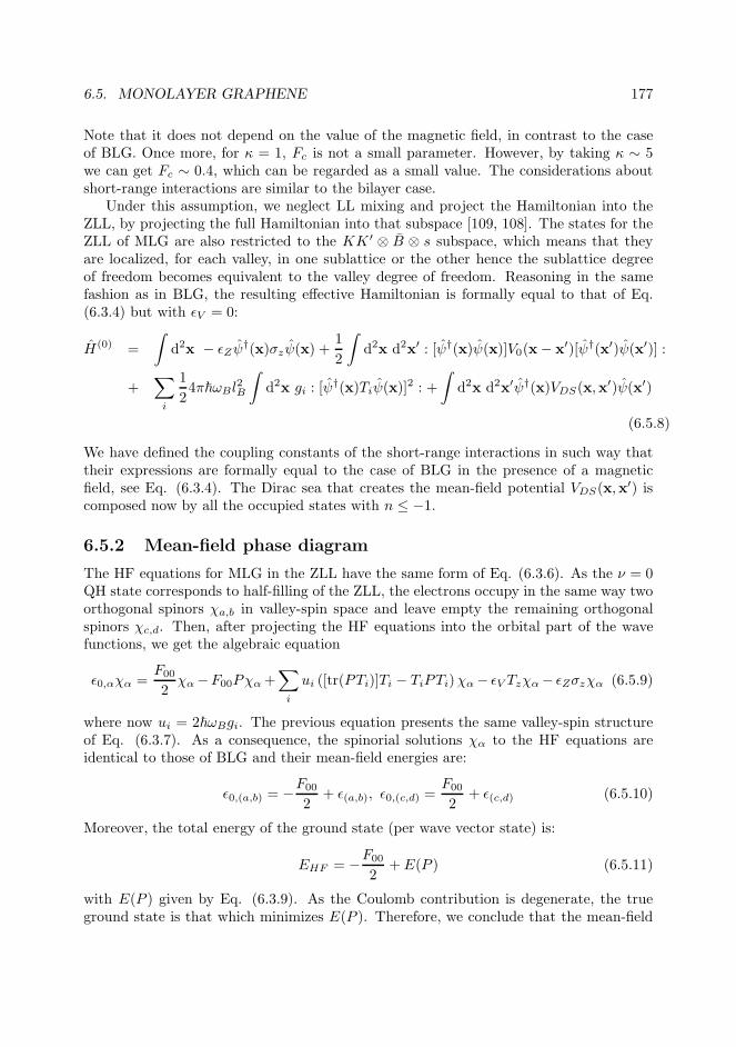
6.5. MONOLAYER GRAPHENE 177
Note that it does not depend on the value of the magnetic field, in contrast to the caseof BLG. Once more, for κ = 1, Fc is not a small parameter. However, by taking κ ∼ 5we can get Fc ∼ 0.4, which can be regarded as a small value. The considerations aboutshort-range interactions are similar to the bilayer case.
Under this assumption, we neglect LL mixing and project the Hamiltonian into theZLL, by projecting the full Hamiltonian into that subspace [109, 108]. The states for theZLL of MLG are also restricted to the KK ′ ⊗ B ⊗ s subspace, which means that theyare localized, for each valley, in one sublattice or the other hence the sublattice degreeof freedom becomes equivalent to the valley degree of freedom. Reasoning in the samefashion as in BLG, the resulting effective Hamiltonian is formally equal to that of Eq.(6.3.4) but with ǫV = 0:
H(0) =
∫
d2x − ǫZψ†(x)σzψ(x) +
1
2
∫
d2x d2x′ : [ψ†(x)ψ(x)]V0(x− x′)[ψ†(x′)ψ(x′)] :
+∑
i
1
24π~ωBl
2B
∫
d2x gi : [ψ†(x)Tiψ(x)]
2 : +
∫
d2x d2x′ψ†(x)VDS(x,x′)ψ(x′)
(6.5.8)
We have defined the coupling constants of the short-range interactions in such way thattheir expressions are formally equal to the case of BLG in the presence of a magneticfield, see Eq. (6.3.4). The Dirac sea that creates the mean-field potential VDS(x,x
′) iscomposed now by all the occupied states with n ≤ −1.
6.5.2 Mean-field phase diagram
The HF equations for MLG in the ZLL have the same form of Eq. (6.3.6). As the ν = 0QH state corresponds to half-filling of the ZLL, the electrons occupy in the same way twoorthogonal spinors χa,b in valley-spin space and leave empty the remaining orthogonalspinors χc,d. Then, after projecting the HF equations into the orbital part of the wavefunctions, we get the algebraic equation
ǫ0,αχα =F00
2χα−F00Pχα+
∑
i
ui ([tr(PTi)]Ti − TiPTi)χα− ǫV Tzχα− ǫZσzχα (6.5.9)
where now ui = 2~ωBgi. The previous equation presents the same valley-spin structureof Eq. (6.3.7). As a consequence, the spinorial solutions χα to the HF equations areidentical to those of BLG and their mean-field energies are:
ǫ0,(a,b) = −F00
2+ ǫ(a,b), ǫ0,(c,d) =
F00
2+ ǫ(c,d) (6.5.10)
Moreover, the total energy of the ground state (per wave vector state) is:
EHF = −F00
2+ E(P ) (6.5.11)
with E(P ) given by Eq. (6.3.9). As the Coulomb contribution is degenerate, the trueground state is that which minimizes E(P ). Therefore, we conclude that the mean-field

178CHAPTER 6. COLLECTIVE MODES OF THE ν = 0 QUANTUM HALL STATE
phase diagram for the ν = 0 QH state in MLG is the same of BLG for ǫV = 0. Inthat case, the PLP phase of Sec. 6.3.2 changes to a fully interlayer coherent (ILC) phasesince then θV = π/2 and the vector n pointing the polarization in the valley space isfully contained in the plane, n = [cosφv, sinφv, 0]. As the valley degree of freedom isequivalent to the sublattice in the ZLL, this state corresponds to a coherent mixture ofthe two sublattices.
There are experimental evidences that the phase for the ν = 0 QH state of monolayergraphene for zero in-plane component of the magnetic field is also the CAF phase [125],so uz > −u⊥ > 0 as in the bilayer case.
6.5.3 Collective modes
The TDHFA developed for computing the collective modes of BLG is also valid for MLG.In particular, the dispersion relation is still obtained from Eq. (6.4.23) but now thereis only one possible value for the magnetic index, nk = 0. Thus, as the structure inthe valley-spin subspace is the same of the bilayer problem, the building blocks of thedispersion matrix X , Y αkαl,αjαm(k, ω), are now scalars instead of 4× 4 matrices:
Y αkαl,αjαm(k, ω) = Y αkαl,αjαm(k)− (ναk− ναl
)~ω (6.5.12)
with
Y αkαl,αjαm(k) = [F (k) + ∆αkαl ] δαkαjδαlαm
+Q(k)Mαkαl,αjαm (6.5.13)
F (k) ≡ F00 − C00,00(k) = F00
[
1− I0
(
(klB)2
4
)
e−(klB )2
4
]
Q(k) ≡ 2R00,00(k) = e−(klB )2
2
and we have made explicit the isotropy in the wave vector dependence of Y αkαl,αjαm(k).The expression of the function C00,00(k) can be obtained from the results of Appendix K.By the same arguments of Sec. 6.4.2, the collective-mode frequencies are the eigenvalues ofthe matrix X(k) in Eq. (6.4.32), which now is reduced to a 8×8 matrix as Y αkαl,αjαm(k)are scalars. Since the ground states in MLG have the same valley-spin structure that inBLG, all the coefficients ∆αkαl , Mαkαl,αjαm remain identical for every phase. Thus, Eqs.(6.4.38), (6.4.44), (6.4.47) and (6.4.55) can be still used for computing the eigenvalues ofX(k). Moreover, as F (0) = 0 and Q(0) = 1, we recover at zero momentum the analyticalresults previously obtained for the symmetric modes ωS [see discussion accompanyingEq. (6.4.36]. In fact, for MLG, the collective modes within the ZLL can be computedexplicitly at arbitrary momentum k.
Ferromagnetic phase
Following Sec. 6.4.2, there are spin flip excitations and full-flip excitations. Mutatismutandi, the frequencies of the two branches of the spin-flip modes are [see Eq. (6.4.39)and related text]:
~ω±(k) = Y ±(k) = Y ac,ac(k)± Y ac,bd(k) = F (k) + 2ǫZ + 2u⊥ + uz +Q(k) [−uz ∓ 2u⊥](6.5.14)

6.5. MONOLAYER GRAPHENE 179
On the other hand, for the full-flip modes, we get:
~ωbc(k) = Y bc,bc(k) = F (k) + 2ǫZ + 2u⊥ + uz +Q(k)uz (6.5.15)
As ǫV = 0, ωbc(k) = ωad(k).
Full layer-polarized phase
In this phase, there are valley-flip and full-flip modes, see Sec. 6.4.2. The valley-flipmodes are
~ω±(k) = Y ±(k) = Y ac,ac(k)± Y ac,bd(k) = F (k)− 2u⊥ − 3uz +Q(k) [2u⊥ + uz ± 2u⊥](6.5.16)
while the frequency of the full-flip modes is
~ωbc(k) = Y bc,bc(k) = F (k)− 2ǫZ − 2u⊥ − 3uz +Q(k)uz = Y −(k)− 2ǫZ (6.5.17)
and ωad(k) = ωbc(k) + 4ǫZ . In correspondence with the results of Sec. 6.4.2, one of thevalley-flip modes is indeed a spin-flip mode, ωbc(k) = ~ω−(k)− 2ǫZ .
Canted anti-ferromagnetic phase
The equivalent of the spin-flip modes of the CAF phase, Sec. 6.4.2. Following the samesteps leading to the matrix of Eq. (6.4.49), we arrive at the corresponding 2× 2 matrix
Xsf,±(k) =
[
Y ±(k) Y ac,db(k)−Y ac,db(k) −Y ±(k)
]
(6.5.18)
The dispersion relation is obtained from its eigenmodes:
~ωsf,±(k) =
√
[Y ±(k)]2 − 4u2⊥ sin4 θsQ2(k) (6.5.19)
Y ±(k) = F (k) + uz − 2u⊥ +Q(k)[
−uz ∓ 2u⊥ cos2 θs]
On the other hand, for the full-flip modes of Eq. (6.4.51), one gets the analog matrix
Xff(k) =
[
Y bc,bc(k) Y bc,da(k)−Y da,bc(k) −Y da,da(k)
]
(6.5.20)
that gives:
~ωbc,da(k) =
√
[Y bc,bc(k)]2 − 4u2⊥ sin4 θsQ2(k) (6.5.21)
Y bc,bc(k) = F (k) + uz − 2u⊥ +Q(k)[
uz + 2u⊥ sin2 θs]
The remaining mode satisfy ωad,cb(k) = ωbc,da(k) as ǫV = 0.

180CHAPTER 6. COLLECTIVE MODES OF THE ν = 0 QUANTUM HALL STATE
Inter-layer coherent phase
For the ILC phase, we set ǫV = 0 and, consistently, θV = π/2 in Eq. (6.4.55). Followingthe lines of Sec. 6.4.2, an analog computation to the spin-flip modes of the CAF phasegives the equivalent of the valley-flip modes. In particular, their dispersion relation is:
~ωvf,±(k) =
√
[Y ±(k)]2 − (uz − u⊥)2Q2(k) (6.5.22)
Y ±(k) = F (k)− uz − 4u⊥ +Q(k) [uz + 2u⊥ ± (u⊥ + uz)]
Finally, for the full-flip excitations, we get
~ωbc,da(k) = −2ǫZ +
√
[Y −(k)]2 − (uz − u⊥)2Q2(k) = ~ωvf,−(k)− 2ǫZ (6.5.23)
As in the FLP phase, the valley-flip branch − is indeed a full-flip mode. The remainingfull-flip mode is ~ωad,bc(k) = ~ωvf,−(k) + 2ǫZ.
Numerical results
We display here the dispersion relations for the different phases. The results for the F(left panel) and FLP (right panel) phases are shown in Fig. 6.5.3 while the results for theCAF (left) and ILC (right) are shown in Fig. 6.5.3. Their qualitative trends are similarto the symmetric modes S of bilayer graphene; indeed, at k = 0, they have the sameexpression. The dispersion relation of the dynamical instabilities of the CAF and ILCphases, when exist, is quite similar to the case of bilayer graphene (not shown).
6.6 Effects of Landau-level mixing
In this section, we consider the case of suspended samples of bilayer graphene, where κ =1. In this case, Fc & 1 for any realistic value of the magnetic field, so we cannot neglect LLmixing. One possible way to take into account the effects of the LL mixing is the screeningof the Coulomb interaction in the large-N approximation [129, 130, 120, 131, 109], whichleads to an RPA-type screening given by:
V (k) =V0(k)
1−Π0(k, 0)V0(k)(6.6.1)
where
~Π0(k, ω) =∑′
nk,nlαkαl
δαk,αl
2πl2BD0
kl(ω)|A(2)nknl
(k)|2 (6.6.2)
is the non-interacting polarization for the ν = 0 QH state and nk, nl take values for allintegers except −1, as in Eq. (6.2.12). In the same fashion, D0
kl(ω) is the non-interactingtwo-particle propagator, with the non-interacting values for the energies and occupationnumbers. Other approaches allow for LL mixing in the Hartree-Fock formalism (see forinstance Ref. [116]); however, they are not expected to describe correctly the dispersionrelation near k = 0. The polarization Π0(k, ω) is obtained from the non-interacting

6.6. EFFECTS OF LANDAU-LEVEL MIXING 181
0 0.5 1 1.5 2 2.5 3 3.5 4 4.5 5
0.2
0.4
0.6
0.8
1
1.2
1.4
1.6
1.8
2
klB
ω/ω
B
sf, +
sf,−
bc
0 0.5 1 1.5 2 2.5 3 3.5 4 4.5 5
0.2
0.4
0.6
0.8
1
1.2
1.4
1.6
1.8
2
klB
ω/ω
B
vf, +
bc
Figure 6.10: Plot of the collective modes of the ν = 0 QH state in monolayer graphene forthe F and FLP phases. Left: dispersion relation of the F phase with parameters Fc = 0.5,uz = 0.1, u⊥ = −0.05 and ǫZ = 0.2. The two spin-flip modes are plotted in solid blue (+branch) and in dot-dashed red (− branch). The full-flip mode frequency ωbc(k) is plottedis dashed black. Right: dispersion relation of the FLP phase with parameters Fc = 0.5,uz = −0.1, u⊥ = −0.05 and ǫZ = 0.02. The solid blue line is the true valley flip mode(labeled as + in Sec. 6.5.3) and the black dashed line is the full-flip mode ωbc(k).
density-density correlation function, following an analog calculation to that leading to
Eq. (6.4.19) but using the bare vertex and allowing for LL mixing. Here, A(2)nn′(k) is the
bilayer graphene magnetic form factor:
A(2)nn′(k) =
1
2
[
a−n,n′A|n|−2,|n′|−2(k)sgn n sgn n′ + a+n,n′Ann′(k)]
a±n,n′ =√
1± (δn0 + δn1)√
1± (δn′0 + δn′1) (6.6.3)
with Ann′(k) the usual magnetic form factor, given by Eq. (J.1.5). Neglecting the smallcorrections due to the Zeeman effect and the layer voltage, the free static polarizationreads:
Π0(k, 0) = − N
2πl2B
f(klB)
~ωB(6.6.4)
f(klB) =
∞∑
nk=0
∞∑
nl=2
2|A(2)nk,−nl
(k)|2√
nk(nk − 1) +√
nl(nl − 1)
where N = 4 is the number of the valley-spin components of the field, which is expected tobe a sufficiently large value to provide a good approximation [130, 131, 109]. The function
f(x) is dimensionless as |A(2)nknl(k)|2 only depends on the value klB, with k = |k|. The
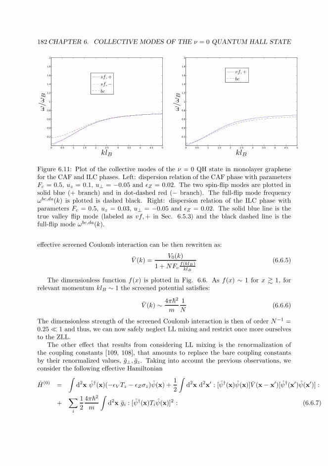
182CHAPTER 6. COLLECTIVE MODES OF THE ν = 0 QUANTUM HALL STATE
0 0.5 1 1.5 2 2.5 3 3.5 4 4.5 5
0.2
0.4
0.6
0.8
1
1.2
1.4
1.6
1.8
2
klB
ω/ω
B
sf, +
sf,−
bc
0 0.5 1 1.5 2 2.5 3 3.5 4 4.5 5
0.2
0.4
0.6
0.8
1
1.2
1.4
1.6
1.8
2
klB
ω/ω
B
vf, +
bc
Figure 6.11: Plot of the collective modes of the ν = 0 QH state in monolayer graphenefor the CAF and ILC phases. Left: dispersion relation of the CAF phase with parametersFc = 0.5, uz = 0.1, u⊥ = −0.05 and ǫZ = 0.02. The two spin-flip modes are plotted insolid blue (+ branch) and in dot-dashed red (− branch). The full-flip mode frequencyωbc,da(k) is plotted is dashed black. Right: dispersion relation of the ILC phase withparameters Fc = 0.5, uz = 0.03, u⊥ = −0.05 and ǫZ = 0.02. The solid blue line is thetrue valley flip mode (labeled as vf,+ in Sec. 6.5.3) and the black dashed line is thefull-flip mode ωbc,da(k).
effective screened Coulomb interaction can be then rewritten as:
V (k) =V0(k)
1 +NFcf(klB)klB
(6.6.5)
The dimensionless function f(x) is plotted in Fig. 6.6. As f(x) ∼ 1 for x & 1, forrelevant momentum klB ∼ 1 the screened potential satisfies:
V (k) ∼ 4π~2
m
1
N(6.6.6)
The dimensionless strength of the screened Coulomb interaction is then of order N−1 =0.25 ≪ 1 and thus, we can now safely neglect LL mixing and restrict once more ourselvesto the ZLL.
The other effect that results from considering LL mixing is the renormalization ofthe coupling constants [109, 108], that amounts to replace the bare coupling constantsby their renormalized values, g⊥, gz. Taking into account the previous observations, weconsider the following effective Hamiltonian
H(0) =
∫
d2x ψ†(x)(−ǫV Tz − ǫZσz)ψ(x) +1
2
∫
d2x d2x′ : [ψ†(x)ψ(x)]V (x− x′)[ψ†(x′)ψ(x′)] :
+∑
i
1
2
4π~2
m
∫
d2x gi : [ψ†(x)Tiψ(x)]
2 : (6.6.7)
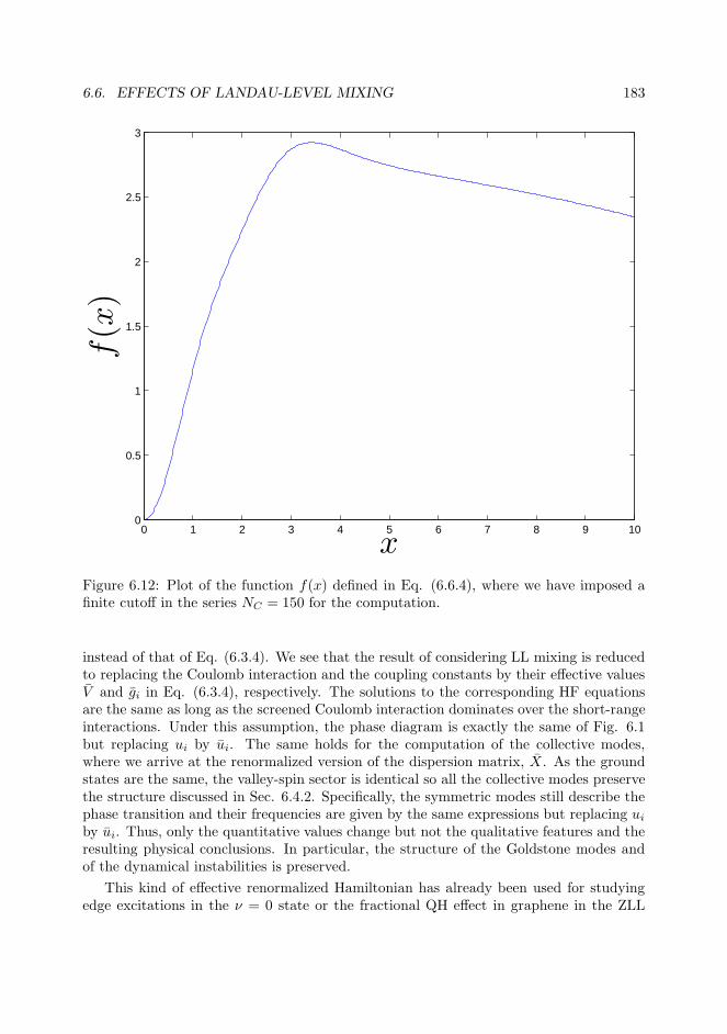
6.6. EFFECTS OF LANDAU-LEVEL MIXING 183
0 1 2 3 4 5 6 7 8 9 100
0.5
1
1.5
2
2.5
3
x
f(x
)
Figure 6.12: Plot of the function f(x) defined in Eq. (6.6.4), where we have imposed afinite cutoff in the series NC = 150 for the computation.
instead of that of Eq. (6.3.4). We see that the result of considering LL mixing is reducedto replacing the Coulomb interaction and the coupling constants by their effective valuesV and gi in Eq. (6.3.4), respectively. The solutions to the corresponding HF equationsare the same as long as the screened Coulomb interaction dominates over the short-rangeinteractions. Under this assumption, the phase diagram is exactly the same of Fig. 6.1but replacing ui by ui. The same holds for the computation of the collective modes,where we arrive at the renormalized version of the dispersion matrix, X. As the groundstates are the same, the valley-spin sector is identical so all the collective modes preservethe structure discussed in Sec. 6.4.2. Specifically, the symmetric modes still describe thephase transition and their frequencies are given by the same expressions but replacing uiby ui. Thus, only the quantitative values change but not the qualitative features and theresulting physical conclusions. In particular, the structure of the Goldstone modes andof the dynamical instabilities is preserved.
This kind of effective renormalized Hamiltonian has already been used for studyingedge excitations in the ν = 0 state or the fractional QH effect in graphene in the ZLL
184CHAPTER 6. COLLECTIVE MODES OF THE ν = 0 QUANTUM HALL STATE
[124, 132]. It can been also applied to study the ν = 0 state for MLG [109, 124].
6.7 Experimental remarks
We make here some experimental remarks, following the results quoted in Sec. 6.3.2. Thevalue of the parameters u⊥, uz is such that uz > −u⊥ > 0 so the state is in the CAFphase for ǫZ = ǫV = 0. All the phases of Fig. 6.1 can be explored by varying the in-planecomponent of the magnetic field or the layer voltage. On the other hand, we see fromEqs. (6.4.54), (6.4.59) that the conditions for the appearance of the unstable modes forboth CAF and PLP phases are
ǫ2Z2u⊥
> u⊥ + uz, (CAF) (6.7.1)
u2z > u2⊥ + ǫ2Z , (PLP)
Interestingly, the saturation of the two previous inequalities correspond to the boundarybetween the PLP and CAF phases for ǫV = 0 (ǫZ = 0). The first condition is unlikelyto be achieved from the arguments displayed above. The second condition, however, iscompatible with the values expected the coupling constants. Let’s imagine that the in-plane magnetic field and the layer voltage are such that the system is initially in the PLPphase. If we now reduce suddenly the layer voltage sufficiently enough for the instabilitycondition of the PLP phase to be fulfilled, then we would be able to observe this dynamicalinstability, in a similar way to the BH laser effect described in Chapter 4. Future workshould address this issue more deeply, exploring the possible experimental consequencesof the appearance of the dynamical instability.
On the other hand, another possible interesting feature is that the energy gap of thesymmetric modes is easily manipulable by tuning the in-plane component of the magneticfield or the layer voltage as they do not depend on the strength of the Coulomb interaction.
The above comments also apply to monolayer graphene except that, unfortunately,there is not an equivalent of the layer voltage so we cannot reproduce the mentionedprotocol for observing the dynamical instability.
6.8 Conclusions and outlook
In this chapter, we have studied the ν = 0 QH state within a mean-field Hartree-Fockapproach restricted to the zero-energy Landau level. We have reproduced the mean-field phase diagram of the ν = 0 QH state of Ref. [109] by solving the self-consistentHartree-Fock equations. Within the time-dependent Hartree-Fock approximation, wehave computed the intra-LL collective modes, that in the limit of zero momentum canbe obtained analytically. In particular, the lowest-energy modes that describe the phasetransition are the symmetric modes, corresponding to a symmetric combination of exci-tations conserving the magnetic number. We have seen that, at the boundary betweenthe ferromagnetic and the fully layer-polarized phases, there is a gapless mode, resultingfrom a residual symmetry [see Eq. (6.4.43)] that can be regarded as a remanent of the
6.8. CONCLUSIONS AND OUTLOOK 185
broken SO(5) symmetry described in Ref. [114]. In respect to the boundary between thecanted anti-ferromagnetic and the partially layer-polarized phases, a similar gapless modeappears. Interestingly, we have seen that these phases can present dynamical instabilities.Although the dynamical instability of the CAF phase is unlikely to be observed since itrequires u⊥ + uz < 0 and this condition is incompatible with the current experimentalobservations, we have discussed in Sec. 6.7 a possible protocol for the observation ofthe dynamical instability associated to the PLP phase. Importantly, we remark that thepossible appearance of such unstable modes results from the short-range valley/sublatticeinteractions. Another interesting feature is that the gap of the symmetric modes is easilytunable by varying the in-plane magnetic field or the layer voltage.
The performed calculations are straightforwardly translated to monolayer graphene,due to the formal analogy of the short-range interactions. We have found that most ofthe conclusions of the previous paragraph still hold in the monolayer scenario. We alsohave analyzed the effects of LL mixing and we have accounted them by screening thelong-range Coulomb interaction and renormalizing the coupling constants of the short-range interactions, following Ref. [109]. The resulting effective Hamiltonian is formallysimilar to that previously considered for the calculations and hence, the phase diagramand the collective modes present the same structure as that discussed above.

186CHAPTER 6. COLLECTIVE MODES OF THE ν = 0 QUANTUM HALL STATE

Part IV
Global conclusions
187


Chapter 7Global conclusions and future
perspectives
In this section we briefly summarize the content of this thesis, remarking the most im-portant results and discussing future perspectives. In the first part of the thesis, we haveexplored the implementation of gravitational analogs in Bose-Einstein condensates. Afteran introductory chapter on the matter, we have reported numerical simulations of the for-mation of a black-hole configuration in a realistic setup. Specifically, we have studied theprocess whereby an initially confined condensate starts leaking after the lowering of theoptical lattice that acts as an initial confining agent. We have first considered the prob-lem in a slightly idealized model in order to understand the main features of the system.We have seen that, under certain conditions (broad conduction bands, adiabatic evolutionand chemical potential near the bottom of the conduction band) a quasi-stationary black-hole configuration is achieved. After this training, we have switched to a realistic casewhere we have confirmed the previous observations. In addition, for the realistic opticallattice with a Gaussian envelope, we have observed and theoretically explained that thesonic horizon is precisely formed at the maximum of the envelope. Above the reachedblack-hole configuration, we have made some preliminary calculations of the Hawkingspectrum. We have seen that, whenever the top of the conduction band is below theHawking frequency, a highly non-thermal peaked structure appears near the top of theconduction band, which could be a promising scenario for an eventual detection of theHawking effect.
Thus, we conclude from the results of the simulations that the considered protocolis a good candidate to produce a quasi-stationary black-hole configuration in achievableexperimental setups. However, we remark the preliminary character of the results forthe Hawking spectrum. A more detailed work should address the problem in the future,taking into account the (weak) time-dependence of the background and the finite sizeof the subsonic region. Also, an adapted calculation should be performed for this setupas the quantum state of the system in the quasi-stationary regime is the time evolution
189
190 CHAPTER 7. GLOBAL CONCLUSIONS AND FUTURE PERSPECTIVES
of the initial thermal equilibrium state, which could probably lead to an integration ofthe time-dependent BdG equations, requiring much harder numerical computations thanthose presented here. Apart from the gravitational analogy, the quasi-stationary blackhole here studied could also be interesting in quantum transport scenarios since it providesa quasi-stationary supersonic current with a very well defined velocity.
In the third chapter of the thesis we have addressed the existence of criteria for thedetection of the spontaneous Hawking radiation. Borrowing some ideas from quantumoptics, we have proposed the violation of Cauchy-Schwarz type inequalities as a signatureof quantum behavior. In particular, we have argued that the violation of the Cauchy-Schwarz inequality involving the outgoing channels associated to the Hawking effect is asmoking gun of the presence of the spontaneous Hawking signal since stimulated Hawkingradiation or linearized coherent motion above the condensate wave function are not able toproduce such violation just by themselves. We have compared the proposed criterion withthe generalized Peres-Horodecki criterion; we have found that, under typical assumptions,both criteria become equivalent. After that, we have presented a discussion on the possibleexperimental implementation. Importantly, we have found that only the violation ofquadratic Cauchy-Schwarz violations can be detected due to the different spatial locationof the asymptotic regions. The numerical results show, however, that this does notrepresent a major limitation in practice for the detection of the Hawking effect. Also,as noticed before, all the above criteria are equivalent under general conditions and,besides, the quadratic Cauchy-Schwarz violation is indeed a signal of quantum behaviorby itself. The results of this chapter of great importance since they provide the theoreticalground for the implementation of experimental detection schemes. Apart from the directimplications for the detection of the Hawking effect, the content of this chapter can alsobe of interest for other fields such as quantum optics, quantum information physics or inthe broader topic of bosonic condensates.
The last chapter of the gravitational analog part is devoted to the study of the so-calledblack-hole laser, formed by a black hole-white hole pair. By integrating the correspondingtime-dependent Gross-Pitaevskii equation, we have analyzed the long-time behavior ofthe system, where the instability has grown up to saturation. On the one hand, we haveconfirmed the theoretical predictions for the unstable behavior at short times and forthe long-time stationary regime, in which the system reaches the non-linear ground statesolution. On the other hand, we have extensively characterized a new regime of continuousemission of solitons, where the system is sufficiently unstable to keep oscillating in such away that emits perfectly periodic trains of solitons into the upstream region. A comparisonwith standard laser devices suggests that the periodic emission of solitons is the actualblack-hole laser effect. The results here presented can be interesting in several fields. Forinstance, the “evaporation” of the horizons caused by the evolution towards the non-linearground state solution can help to understand the much complex case of the evaporationin an actual cosmological black hole due to the spontaneous Hawking effect. In respectto the continuous emission of solitons, they represent a non-linear analog of an opticallaser device, with potential interest in quantum transport or atomtronics scenarios. Inthe future, new theoretical works should provide a better understanding of the regime ofcontinuous emission of solitons. The effect of quantum fluctuations above the coherentsoliton laser regime is an open subject that should also be addressed. In respect to the
191
experimental part, it is expected that forthcoming experiments will be able to characterizethe long-time non-linear behavior of the black-hole laser. We remark that most of theresults presented in this chapter can be directly translated to other analog scenarios suchas quantum fluids of light, for instance.
In the fifth chapter, we have switched, within the same context of boson gases, to theopposite limit of a thermal cloud above the critical temperature. We have studied theresponse induced in the system by the introduction of a temporal Bragg pulse. We haveshown using both classical and quantum descriptions that, whenever the local-densityapproximation is valid, interactions are negligible and the pulse is sufficiently short, theformed periodic density pattern decays to the equilibrium configuration. However, thisdamping mechanism is not due to the collisional relaxation of the collective modes usuallydescribed in the standard literature but rather to the thermal disorder of the particles. Inparticular, the decay is given by a Gaussian function with a characteristic time that onlydepends on the temperature, the mass of the atoms and the wave vector of the latticepotential. We have discussed thoroughly the validity of the approximations made and thelink between the classical and quantum calculations. We have also shown that, indeed,this decay is a very general phenomenon that appears under quite general grounds forany spatially periodic pulse. A very good agreement is found between the theoreticalpredictions and the experimental data provided by the Technion group. The developedformalism can be translated to other systems such as Fermi gases at sufficiently hightemperature or the thermal component of a Bose gas below the critical temperaturewhenever the picture of non-interacting atoms holds. A future work could try to extendthis formalism to the phonons above the condensate.
Finally, we have devoted the content of the last chapter to a very different system:quantum Hall effect on graphene. In particular, we have studied the ν = 0 quantumHall state of bilayer graphene. Using a mean-field Hartree-Fock approach, we have re-derived the corresponding mean-field phase diagram. After that, we have computed thecollective modes within the zero Landau level trough the time-dependent Hartree-Fockapproximation. Among the most remarkable results, we have found that at the boundarybetween the full layer-polarized and the ferromagnetic phases a gapless mode appearsresulting from an accidental symmetry that can be regarded as a remanent of a brokenSO(5) symmetry. Interestingly, we have seen that the canted anti-ferromagnetic andpartially layer-polarized phases can present dynamical instabilities. We emphasize thecrucial role played by the valley/sublattice short-range interactions in the appearance ofsuch instabilities. The theoretical calculations previously developed are easily applied tomonolayer graphene. Following previous works on the field, we have discussed the effectsof LL mixing and we have taken them into account, arriving at an effective Hamiltonianformally similar to that previously considered, which preserves the structure of the phasediagram and of the collective modes and hence, the resulting physical conclusions are thesame. One interesting feature is that the gap of the symmetric modes does not dependon the strength of the Coulomb interaction and it can be easily manipulated with thehelp of the layer voltage or the in-plane component of the magnetic field. We have alsodiscussed a possible protocol to observe the dynamical instability of the PLP phase; thisissue could be further investigated in the future.
192 CHAPTER 7. GLOBAL CONCLUSIONS AND FUTURE PERSPECTIVES
Part V
Appendices
193

Appendix A1D solutions of the Gross-Pitaevskii
equation
We review in this Appendix the solutions to the 1D stationary GP equation, in similarterms to Refs. [22, 23, 85]. Using the same amplitude-phase decomposition that leads toEq. (1.2.25), we can write the 1D time-independent GP equation as:
dJ
dx= 0 (A.0.1)
µA(x) = − ~2
2m
d2A
dx2+
1
2mv2(x)A + V (x)A + gA3 ,
where v, J are the 1D velocity and current. The first equation tells us that the currentis constant. Specifically, A2(x)v(x) = J and thus we can rewrite the equation for theamplitude as:
µA(x) = − ~2
2mA′′ +
mJ2
2A3+ V (x)A+ gA3 , (A.0.2)
where ′ denotes spatial derivative. We note that, if J 6= 0, neither the amplitude or theflow velocity vanish and hence we can safely choose J > 0 so v(x) > 0 at every point.
We only consider in this Appendix the case in which the external potential is zeroor constant, where in the latter case we can absorb it in the definition of the chemicalpotential. The importance of this particular case is based on that it is the most consideredscenario in analog condensed systems due to its analytical simplicity. First, we look forhomogeneous solutions corresponding to plane waves, A(x) = A0, which are given by thezeros of:
gn30 − µn2
0 +mJ2
2= 0, n0 = A2
0 (A.0.3)
195

196 APPENDIX A. 1D SOLUTIONS OF THE GROSS-PITAEVSKII EQUATION
This equation only has real solutions whenever:
J ≤√
8µ3
27mg2(A.0.4)
Suppose now that we find one solution to the previous equation, let’s say n0 = nb. Then,after rescaling all the previous magnitudes we obtain:
0 = X3 − µX2 +v2b2
= (X − 1)
(
X2 − v2b2X − v2b
2
)
(A.0.5)
X =n0
nb=c20c2b, vb =
J
nbcb, µ = 1 +
v2b2
(A.0.6)
where c0,b is the sound speed associated to the density n0,b, c0,b =√
gn0,b/m. It isimmediate from here to obtain the other two roots for Eq. (A.0.5):
X =v2b ±
√
v4b + 8v2b4
(A.0.7)
The previous equation has two solutions for n0, one positive and one negative, the latterunphysical so we only consider the positive one, which we label as np.
As explained in the main text, a solution is subsonic whenever c > v and supersonicwhenever c < v, where c is the sound speed and v the flow velocity. Taking into accountthat nbvb = J , we find that vb =
vbcb
is the Mach number for the particular solution nb. For
vb ≷ 1 we have a supersonic (subsonic) solution. For the other one, taking into accountthat nbvb = J = npvp, we find that its Mach number is:
vpcp
=z
(1 +√1 + z)
32
(A.0.8)
where we have introduced the dimensionless quantity z ≡ 8/v2b . As the function f(z) =z2/3 − 1 −
√1 + z increases monotonically for z > 0, it only has one zero, at z = 8
or, equivalently, vb = 1. Then, if vb ≶ 1, vp/cp ≷ 1 and thus, we always have onesolution subsonic and one supersonic. The limit case vb = 1 presents a doubly degeneratedsolution. In the following, we take nb as the subsonic solution and np as the supersonicone, satisfying nb > np.
Non-homogeneous solutions can also appear. In order to compute them, we note thatEq. (A.0.2) can be regarded as the classical motion equation of a particle in a certainpotential W (A). Integrating the equation, we obtain:
1
2A′2 +W (A) = EA (A.0.9)
W (A) =m
~2
(
mJ2
2A2+ µA2 − g
2A4
)
where EA is the analogous to the mechanical energy of the particle and we denote it asthe amplitude energy. We plot the potentialW (A) in Fig. A.1. The local minimum corre-sponds to the supersonic homogeneous solution with amplitude Ap =
√np (which means

197
Ap
Ab
A
W(A
)
A
A′
Ap Ab
Figure A.1: Left plot: representation of the amplitude potential W (A) (black solid line).We depict some values of the amplitude energy EA corresponding to qualitatively differentsolutions; E =W (Ab) is plotted in black thick line, W (Ap) < EA < W (Ab) is plotted insolid blue line, EA > W (Ab) is plotted in red dashed line and EA < W (Ap) is plotted ingreen dashed-dotted line. The homogeneous solutions A = Ab and A = Ap are markedwith a black dot. Right panel: orbits in the space (A,A′) associated to the values ofthe amplitude energy shown in the left panel, which can be obtained from the identityA′2 = 2[EA −W (A)]. The horizontal black line marks A′ = 0.
that it is an stable fixed point) and the local maximum to the subsonic homogeneoussolution with amplitude Ab =
√nb (which means that it is an unstable fixed point).
We can further rewrite the previous identity in terms of the density as:
n′2 = 4g(n− n1)(n− n2)(n− n3), g ≡gm
~2(A.0.10)
where ni, i = 1, 2, 3 are the roots of the polynomial
gn3 − 2µn2 + 2~2
mEAn−mJ2 = g(n− n1)(n− n2)(n− n3) = 0 (A.0.11)
which is equivalent to find the zeros of the equation W (A) = EA. We distinguish severalcases according to the value of the amplitude energy EA.
For W (Ap) < EA < W (Ab), the three roots are real (blue line of left Fig. A.1)and we take them such 0 < n1 < n2 < n3. We first consider the oscillating solutionn1 < n(x) < n2, corresponding to the closed blue line of right Fig. A.1. Integrating Eq.(A.0.10), we find:
∫
dn
2√
(n− n1)(n2 − n)(n3 − n)= ±
√
g(x− x0) (A.0.12)
with x0 some integration constant. The solution of the previous indefinite integral is givenin term of elliptical functions [49, 133]. The phase of the wave function can be obtained

198 APPENDIX A. 1D SOLUTIONS OF THE GROSS-PITAEVSKII EQUATION
by integrating the relation ~θ′(x)/m = v(x) = J/n(x). Putting all together, we get:
Ψ0(x) = A(x)eiθ(x) (A.0.13)
n(x) = n1 + (n2 − n1)sn2(√
g(n3 − n1)(x − x0), ν), ν =n2 − n1
n3 − n1
θ(x) = θ(0) +mJ
~n1
√
g(n3 − n1)
× Θ(
√
g(n3 − n1)(x− x0),−√
g(n3 − n1)x0, n1, n2, n3, ν)
Θ(u2, u1, n1, n2, n3, ν) = Π
(
am(u2, ν), 1 −n2
n1, ν
)
−Π
(
am(u1, ν), 1−n2
n1, ν
)
For understanding better the notation in the previous equation, we briefly review someconcepts about elliptic functions. The function sn(u, ν) is a Jacobi elliptic function. It isdefined as sn(u, ν) = sin (am(u, ν)), where am(u, ν) is the inverse function of F (φ, ν),
F (φ, ν) ≡∫ φ
0
dϕ√
1− ν sin2 ϕ(A.0.14)
so u = F (am(u, ν), ν). The function F (φ, ν) is known as the incomplete elliptic integralof the first kind. As a consequence of the previous relations, sn(u, ν) is a periodic functionwith period 4K(ν), K(ν) = F (π2 , ν) being the complete elliptic integral of the first kind.The function Π(φ,m, ν) is the incomplete elliptic integral of the third kind:
Π(φ,m, ν) ≡∫ φ
0
dϕ
(1−m sin2 ϕ)√
1− ν sin2 ϕ(A.0.15)
On the other hand, for W (Ap) < EA < W (Ab) and n(x) > n3, the solution growsindefinitely, see the blue orbit for A > Ab in right plot in Fig. A.1). Moreover, for highvalues of n, we have n′ ∝ n3/2 which implies that the solution blows up at some finitevalue xbu as n(x) ∼ (x − xbu)
−2. The same reasoning holds for EA < W (Ap) (greendashed-dotted line of Fig. A.1) or EA > W (Ab) (red dashed line of Fig. A.1). We do notcare about these exploding solutions since they do not appear in this work.
Finally, we consider the degenerate cases EA = W (Ap) and EA = W (Ab). For EA =W (Ap), we have n1 = n2 = np. One possible solution corresponds to the stable fixedpoint of the homogeneous supersonic solution n(x) = np:
Ψ0(x) =√npe
iqpx, qp =mvp~
(A.0.16)
with qp the supersonic momentum. The other possible solution corresponds to n(x) > n3,which blows up as explained.
The other degenerate case is EA = W (Ab), where the roots satisfy n2 = n3 = nb andn1 = nbv
2b . For n(x) = nb, the solution is the subsonic plane wave
Ψ0(x) =√nbe
iqbx, qb =mvb~
(A.0.17)
A.1. BLACK-HOLE TYPE SOLUTIONS 199
For n(x) 6= nb, we get from Eq. (A.0.12)∫
dX
2√
(X − 1)2(X − v2b )= ±x− x0
ξb(A.0.18)
X =n
nb, ξb =
1√gnb
ξb being the healing length associated to the subsonic density. For X < 1, i.e., n(x) < nb,we obtain:
n(x) = nb
[
v2b + (1− v2b ) tanh2
(
√
1− v2bx− x0ξb
)]
(A.0.19)
which is just the same of Eq. (A.0.13) taking into account that sn(u, 1) = tanh(u). Thephase of the wave function can be obtained analytically in a simple form and we can writethe total wave function as:
Ψ0(x) = nbeiqbxeiθ0
[
√
1− v2b tanh
(
√
1− v2bx− x0ξb
)
− ivb
]
(A.0.20)
being θ0 some constant phase. This solution represents a soliton solution with zero velocity[27]. We note that vb < 1 since it is the Mach number of a subsonic solution.
On the other hand, taking X > 1 in Eq. (A.0.18), we obtain the so-called shadowsoliton solution [85], which gives:
Ψ0(x) = nbeiqbxeiθ0
[
√
1− v2bcotanh
(
√
1− v2bx− x0ξb
)
− ivb
]
(A.0.21)
Although, as previously discussed, this solution blows up at a finite value of x, it appearswhen studying the BH lasers of Chapter 4.
From all the previous solutions, the most relevant ones for BH configurations arethe supersonic wave function (A.0.16), which appears in the supersonic region of a BH;the subsonic soliton (A.0.20), which typically appears in the subsonic region and theoscillating solution of Eq. (A.0.13) that can appear in the scattering region between thetwo asymptotic regions.
A.1 Black-hole type solutions
We now compute the GP wave functions for the different BH configurations of Sec. 1.3. Inthe flat-profile type configurations, the wave function is trivial since it is a plane wave. Wefocus on the more interesting cases of non-homogeneous wave functions. In the following,we assume that the condition (A.0.4) is satisfied in both asymptotic regions. In order tosimplify the notation, we rescale the wave function to the density of the subsonic regionΨ0 → √
nuΨ0 and set units such ~ = m = cu = 1, with cu the subsonic sound speed. Inthese units, we have that the amplitude potential W (A) is determined only by the valueof the subsonic flow velocity vu, which we denote in the following as simply v, since inthese units the current is just J = v and the chemical potential is µ = 1 + v2/2:
W (A) =v2
2A2+
(
1 +v2
2
)
A2 − A4
2(A.1.1)
200 APPENDIX A. 1D SOLUTIONS OF THE GROSS-PITAEVSKII EQUATION
The amplitude of the subsonic homogeneous solution now corresponds to A = 1. As itrepresents an unstable fixed point, it can only be reached at x→ −∞. On the other hand,the stable point corresponding to the supersonic homogeneous solution can be extractedfrom Eq. (A.0.7):
Ap =
√
v2 +√v4 + 8v2
4< 1 (A.1.2)
since v < 1 is also the subsonic Mach number. In all the cases considered in the rest ofthis section, the GP wave function in the subsonic region is the soliton solution of Eq.(A.0.20), which in our units can be rewritten as:
Ψ0(x) = (γ(x) + iv) eiqxeiθ0 ,
γ(x) =√
1− v2 tanh[
√
1− v2(x0 − x)]
, (A.1.3)
where we have conveniently multiplied the original wave function by −1. The amplitudeenergy of Eq. (A.0.9) for the soliton subsonic solution is simply given by:
EA =W (1) =1
2+ v2 (A.1.4)
If we look at the x coordinate as a time coordinate, our GP solution starts at x = −∞in the subsonic solution (A.1.3) and ends at x = ∞ in the supersonic plane wave solution.As the amplitude energy EA is a conserved quantity for homogeneous problems, we needsome inhomogeneity in order to switch from one asymptotic solution to the other one.This can be achieved by introducing a scattering structure such as a potential or aninhomogeneous coupling constant.
We note that, for these models, the Hawking temperature [57, 63] can be obtainedanalytically. The expression for the Hawking temperature, after momentarily restoringdimensions, is given by:
kBTH =~
2π
d
dx[v(x) − c(x)]x=xH
(A.1.5)
where x = xH is the location of the horizon, v(xH) = c(xH). Going back to our dimen-sionless system of units, we have that c(x) = A(x) and then the continuity equation givesc2(x)v(x) = v. Thus, the local Mach number is
M(x) ≡ v(x)
c(x)=
v
c3(x)(A.1.6)
and then we find that M(xH) = 1 implies A(xH) = c(xH) = v13 , which gives the location
of the horizon. From all the previous results, we can rewrite the equation for the Hawkingtemperature as simply:
TH = − 3
2πc′(x = xH) =
3
2π
√
2[
EA −W (v13 )]
(A.1.7)

A.1. BLACK-HOLE TYPE SOLUTIONS 201
where TH is in units of mc2u/kB. In particular, if the horizon is placed in the region wherethe GP solution is given by the soliton solution of Eq. (A.1.3), we find:
TH =3
2π
(
1− v23
)
√
1− v43 <
3
2π<
1
2(A.1.8)
The importance of the Hawking temperature is that, in most non-resonant configurations,the Hawking spectrum is described reasonably well by a Planck distribution in frequencieswith effective temperature TH , see Refs. [57, 63] for further details.
A.1.1 Delta-barrier configuration
By introducing a potential of the form V (x) = Zδ(x), we create a discontinuity in thederivative of Ψ0(0), Ψ
′0(0
+)−Ψ′0(0
−) = 2ZΨ0(0), which amounts to A′0(0
+)−A′0(0
−) =2ZA0(0) in terms of the amplitudes. In the rest of the space we have the same homo-geneous problem previously discussed. In this way, for x < 0, the wave function is thesame soliton solution of Eq. (A.1.3). For x > 0, the solution is the supersonic plane wave,whose amplitude is given by Ap, see Eq. (A.1.2). Joining both solutions gives
Ψ0(x) = [γ(x) + iv] eiqxeiθ0 , x < 0
Ψ0(x) = Apeivpx, vp = v/A2
p, x > 0 (A.1.9)
We take the phase θ0 such that Ψ0(0) is real and x0 such that the amplitude of the wavefunction is continuous at x = 0,
eiθ0 =γ(0)− iv√
γ2(0) + v2, x0 =
1√1− v2
arctanh
√
A2p − v2
1− v2
(A.1.10)
A.1.2 Waterfall configuration
The potential is now a negative step function with amplitude −V0 < 0. For x < 0, wehave the same type of soliton solution. We note that, for x > 0, the amplitude potentialW (A) is different to that of the subsonic region and so its supersonic amplitude. Asthe step potential does not introduce a discontinuity in the amplitude or the derivativesof the wave function, W (A) must be such that its supersonic solution matches with thesoliton solution at x = 0. Then, A′(0) = 0, which implies that the amplitude of the wavefunction at zero must be the minimum of the soliton amplitude A(0) = v, see Eq.(A.1.3).The value of V0 must be such the supersonic amplitude for x > 0 is Ap = v and byconservation of the current J we find that vd = 1/v, vd being the value of the supersonicvelocity. From these considerations, we obtain that the total wave function can be writtenas:
Ψ0(x) =[
v + i√
1− v2 tanh(
√
1− v2x)]
eivx, x < 0
Ψ0(x) = veix/v, x ≥ 0 (A.1.11)

202 APPENDIX A. 1D SOLUTIONS OF THE GROSS-PITAEVSKII EQUATION
A.1.3 Resonant double delta-barrier configuration
This case is quite similar to the δ barrier previously considered but now with a doublebarrier V (x) = Z[δ(x) + δ(x − d)]. We divide the problem in three regions: region 1, forx < 0; region 2, for 0 < x < d and region 3, for x > d. At the boundaries between theregions, the derivative of the amplitude of the wave function is discontinuous due to theδ barriers. In each region, the GP equation reduces to the homogeneous problem given ofEq. (A.0.9), with three different values of the constant EA, labeled as Ei, i = 1, 2, 3. Forx < 0, the solution is again a soliton wave and for x > d, the solution is the homogeneoussupersonic plane wave of Eq. (A.1.9) so E1 =W (1) and E3 =W (Ap). The value of E2 canbe extracted by the discontinuity A′(d+)−A′(d−) = 2ZA(d). Since at x = d+ we have thesupersonic plane wave solution, we find E2 = 2Z2A2
p + E3. The value of E2 must satisfyE2 < E1 because if not, the solution in the region 2 cannot be matched with the solitonin the region 1 as we infer from Fig. A.1. For obtaining an equation for the amplitude atx = 0, A(0), we compute the difference between Eq. (A.0.9) in the regions 1 and 2 andtaking into account the discontinuity in the derivative, A′(0+) − A′(0−) = 2ZA(0), wearrive at:
n′(0−) =∆E
Z− 2Zn(0), ∆E = E2 − E1
n′2(0−) = 4[n(0)− 1]2[n(0)− v2] (A.1.12)
where we have rewritten the equation for A(0) and A′(0−) in terms of the density n(0) =A2(0) and its derivative at x = 0−, n′(0−) = 2A(0)A′(0−). The previous system ofequations has two solutions for n(0) provided that Z takes values in the range Z ∈(Zmin(v), Zmax(v)), where the limits of the range depend only on the value of the subsonicflow speed v. In particular, the value of Zmax(v) is the maximum value that Z can takein such way that the solution is not a exploding one, i.e., E2 ≤ E1:
Zmax(v)) =
√
E1 − E3
2A2p
(A.1.13)
The solution in the region 2 is given in terms of elliptic functions, see Eq. (A.0.13).Specifically, the inter-barrier solution can be written as:
Ψint0 (x) = A(x)eiθ(x) (A.1.14)
n(x) = n1 + (n2 − n1)sn2(√n3 − n1x+ u0, ν), ν =
n2 − n1
n3 − n1
u0 = sgn[n′(0+)] sn−1
√
n(0)− n1
n2 − n1, ν
θ(x) =v
n1√n3 − n1
×
×[
Π
(
am(√n3 − n1x+ u0, ν), 1−
n2
n1, ν
)
−Π
(
am(u0, ν), 1−n2
n1, ν
)]
A.1. BLACK-HOLE TYPE SOLUTIONS 203
where we have chosen the phase such the wave function is real at x = 0, as in the singlebarrier case. Here, sn−1(u, ν) is the inverse function of sn(u, ν), given by:
sn−1(u, ν) = F (arcsin(u), ν) (A.1.15)
By imposing n(d) = A2p, we find that for given values of v and Z, only a discrete number
of solutions exist for the value of the distance between barriers d:
dn =[2n+ 1 + sgn(u1 + u0)]K(ν)− u1 − u0√
n3 − n1
u1 = sn−1
√
A2p − n1
n2 − n1, ν
(A.1.16)
In the previous expression, n = 0, 1, 2 . . . is the number of periods of the density betweenthe barriers. Gathering the solutions of all regions:
Ψ0(x) =
[γ(x) + iv] eiqxeiθ0 , x < 0Ψint
0 (x), 0 < x < d
Apei[vpx+θ(d)], vp = v/A2
p, x > d(A.1.17)
where γ(x), θ0 are chosen such the function is continuous and real at x = 0 and θ(d) isthe phase of Eq. (A.1.14) evaluated at x = d.

204 APPENDIX A. 1D SOLUTIONS OF THE GROSS-PITAEVSKII EQUATION
Appendix BNon-homogeneous Bogoliubov-de
Gennes equations: Lax pair of
equations.
We devote this Appendix to compute the stationary BdG solutions in 1D whenever thewave function Ψ0 is inhomogeneous [when Ψ0 is a plane wave, the BdG solutions aretrivial plane waves, given by Eq. (1.2.42)]. Following Refs. [134, 135, 22], we obtain thesolutions to the 1D time-dependent BdG equations from the following system of equations,known as the Lax pair of equations of the Zhakarov-Shabat problem:
∂
∂x
[
w1(x, t)w2(x, t)
]
=
[
−iλ Ψ∗(x, t)Ψ(x, t) iλ
] [
w1(x, t)w2(x, t)
]
(B.0.1)
∂
∂t
[
w1(x, t)w2(x, t)
]
=
[
iλ2 + i |Ψ(x,t)|22
(
− i2
∂∂x − λ
)
Ψ∗(x, t)(
i2
∂∂x − λ
)
Ψ(x, t) −iλ2 − i |Ψ(x,t)|22
]
[
w1(x, t)w2(x, t)
]
where λ is some constant parameter and Ψ(x, t) a function that depends on space andtime. The previous system of equations is compatible (i.e., the mixed derivatives satisfythe Schwarz lemma) whenever Ψ(x, t) satisfy:
i∂Ψ(x, t)
∂t= −1
2
∂2Ψ(x, t)
∂x2+ |Ψ(x, t)|2Ψ(x, t) (B.0.2)
which means that Ψ(x, t) is a solution of the time-dependent GP equation, expressed ina dimensionless system of units. Moreover, it can be shown that the solutions to the Lax
205
206 APPENDIX B. LAX PAIR OF EQUATIONS
pair of equations (B.0.1) satisfy:
i∂
∂tz(x, t) =
[
− 12
∂2
∂x2 + 2|Ψ(x, t)|2 Ψ2(x, t)
Ψ∗2(x, t) 12
∂2
∂x2 − 2|Ψ(x, t)|2
]
z(x, t)
z(x, t) =
[
w22(x, t)
w21(x, t)
]
(B.0.3)
Thus, we can identify the components of the BdG spinor with the solutions of the Laxpair of equations as u = w2
2 and v = w21 .
We consider now stationary solutions of the GP equation Ψ(x, t) = Ψ0(x)e−iµt. In
that case, we look for stationary solutions to the BdG equations, which take the followingform in terms of the Lax spinors:
[
w1(x, t)w2(x, t)
]
= e−iω2 t
[
eiµ2 tw1(x)
e−iµ2 tw2(x)
]
(B.0.4)
where ω is the corresponding energy. The Lax pair of equations takes then the form:
0 =
i(
λ2 + |Ψ0(x)|22 − µ
2
)
+ iω2(
− i2
∂∂x − λ
)
Ψ∗0(x)
(
i2
∂∂x − λ
)
Ψ0(x) −i(
λ2 + |Ψ0(x)|22 − µ
2
)
+ iω2
[
w1(x)w2(x)
]
∂
∂x
[
w1(x)w2(x)
]
=
[
−iλ Ψ∗0(x)
Ψ0(x) iλ
] [
w1(x)w2(x)
]
(B.0.5)
We see that obtaining the eigenmodes of the BdG equations reduces to integratinga first order system of ODEs, which is easier than the original second order equationcorresponding to the BdG equations. Due to this fact, in some situations we can obtainanalytical solutions. Specifically, we focus on the often considered case where the station-ary GP wave function is a soliton wave, Eq. (A.0.20). For matching the dimensionlessnotation of the Lax equations, we rescale the wave function as Ψ0(x) →
√nbΨ0(x) and
set units such ~ = m = ξb. In order to unify the results with BH solutions, we relabelv = vb and multiply the wave function by −1, obtaining the same formal expression ofEq. (A.1.3). We then look for asymptotic plane wave solutions of the form:
[
w1(x)w2(x)
]
= eik2 x
[
e−i(vx+θ0)
2 w1(x)
ei(vx+θ0)
2 w2(x)
]
(B.0.6)
where w′i(x) → 0 for x→ ±∞ in order to asymptotically match the corresponding plane
wave solutions. We can identify k as the total momentum of the final BdG solution.Inserting the previous ansatz in the spatial Lax equation of (B.0.5) gives
∂
∂x
[
w1(x)w2(x)
]
=
[
−i(
λ− v2
)
− ik2 γ(x)− ivγ(x) + iv i
(
λ− v2
)
− ik2
] [
w1(x)w2(x)
]
(B.0.7)
207
In order to find non-trivial solutions, for x→ ±∞, the determinant of the previous matrixhas to be zero, which gives the condition:
λ =v
2±√
1 +k2
4(B.0.8)
Applying the same reasoning to the time Lax equation of (B.0.5), we find
ω = k(λ+ v/2) (B.0.9)
which is nothing else than the usual dispersion relation of Eq. (1.2.40). By making thefollowing change of variables
w±(x) = w1(x) ± w2(x) (B.0.10)
and deriving to arrive at a second order differential equation, we obtain:
w′′± = −ikw′
± +(
±γ′(x)− (1 − v2) + γ2(x))
w± (B.0.11)
As our soliton solution satisfy γ′(x) = −(1 − v2) + γ2(x) and w′−(−∞) = 0, it follows
w′−(x) = 0 and then, w−(x) = R, with R some constant. Going back to the Lax spatial
equation, we find:
w+(x) = iγ(x) + ik2λ+ v
2
R (B.0.12)
and inverting the relation
w1,2(x) =R
2
(
1± γ(x) + ik2λ+ v
2
)
(B.0.13)
Finally, taking the constant R such the previous solutions are properly normalized planewaves for x → ±∞, the ua,ω(x), va,ω(x) components of the BdG solutions that asymp-totically match the plane wave with wave vector ka are given by:
sa,ω =
[
ua,ω(x)va,ω(x)
]
=Cae
ikax
√
2π|wa|
[
ei(vx+θ0)[
1 + ka
ω
(
ka
2 − iγ(x))]2
e−i(vx+θ0)[
1− ka
ω
(
ka
2 − iγ(x))]2
]
Ca =ω
√
8k2a|ω − vka|(B.0.14)
As mentioned, it is easy to check that these solutions reduce to the corresponding scat-tering channel a for x→ ±∞ (apart from some trivial k-dependent phase).
When considering stationary GP solutions involving elliptic functions such Eq. (A.0.13),we are not able to find the explicit solution from this method and we have to use numeri-cal integration to find the corresponding BdG solutions, which are Bloch type waves sincethe density is periodic. We do not need to compute the BdG solutions for exploding GPsolutions as we never use them.

208 APPENDIX B. LAX PAIR OF EQUATIONS

Appendix CComputation of the scattering matrix
C.1 General case and asymptotic behavior
We explain in this Appendix how to compute the S-matrix elements. For that purpose,we study the matching of the BdG solutions in the asymptotic subsonic and supersonicregions. When considering Eq. (1.2.9) in 1D, we see that we can rewrite the eigenvalueproblem of the BdG equations as a four-dimensional linear system of ODEs:
dσ
dx= D(x, ω)σ, (C.1.1)
σ(x) = [u(x), v(x), u′(x), v′(x)]T
(C.1.2)
where D(x, ω) is a 4× 4 matrix of the form:
D(x, ω) =
[
0 I2
M(x, ω) 0
]
(C.1.3)
M(x, ω) =2m
~2
[
V (x) + 2g|Ψ0(x)|2 − µ− ~ω L(x)L∗(x) V (x) + 2g|Ψ0(x)|2 − µ+ ~ω
]
L(x) = gΨ20(x)
and I2 is the identity matrix in two dimensions. We divide the system in three regions:the subsonic region (x→ −∞), the supersonic region (x→ ∞) and the scattering region(that between the subsonic and supersonic regions). In both asymptotic regions, thesolutions are combinations of the different scattering channels, as explained in Sec. 1.2.3.Writing the matching equations at the points xu → −∞ and xd → ∞ for ω < ωmax:
209
210 APPENDIX C. COMPUTATION OF THE SCATTERING MATRIX
bu−inσu−in,ω (xu) + bu−outσu−out,ω (xu) + bevσev,ω (xu) =
4∑
j=1
bjσi,ω (xu)
4∑
j=1
bjσi,ω (xd) = bd2−inσd2−in,ω (xd) + bd1−inσd1−in,ω (xd) (C.1.4)
+ bd1−outσd1−out,ω (xd) + bd2−outσd2−out,ω (xd)
where σa,ω is a four-component vector of the form:
σa,ω(x) =
[
sa,ω(x)s′a,ω(x)
]
(C.1.5)
In Eq. (C.1.4), σi,ω (x) are four arbitrary independent solutions of the BdG equationsin the scattering region and the index ”ev” labels the real exponential evanescent wavethat exists in the subsonic region (the other real exponential solution is exploding and thenunphysical). Thus, there are 11 amplitudes and 8 restrictions so we only have 3 degrees offreedom. In particular, we can choose these independent amplitudes as the “in” scatteringchannel amplitudes. Writing Eq. (C.1.4) as a linear system of 8 equations:
d = A · bb = [bu−out, bev, b1, b2, b3, b4, bd1−out, bd2−out]
T(C.1.6)
d = bu−in
[
σu−in,ω (xu)0
]
+ bd1−in
[
0σd1−in,ω (xd)
]
+ bd2−in
[
0σd2−in,ω (xd)
]
,
A =
[
−σu−out,ω (xu) −σev,ω (xu) F (xu) 0 00 0 F (xd) −σd1−out,ω (xd) −σd2−out,ω (xd)
]
where F (x) is a 4 × 4 matrix whose columns are the four linearly independent solutionsσi(x) in the scattering region. The matrix F is often denoted in the literature as thefundamental matrix of the system of equations.
In practice, we can solve the previous matching equations by choosing the pointsxu, xd sufficiently deep in the regions where the wave function tends to a plane wave.Specifically, in the cases considered in the present work, when the wave function is notdirectly the homogeneous subsonic plane wave as in the flat profile type configurations, thewave function tends to a plane wave with exponentially small corrections in the subsonicregion [see the soliton wave function of Eq. (A.1.3)], and it is a perfect plane wave in thesupersonic region for a finite value of xd. The fundamental matrix F , if it cannot obtainedanalytically, is computed numerically by integrating the 4×4 system of equations (C.1.1)for four independent initial conditions. We note that the fundamental matrices of twopoints x1, x2 are connected through the so-called transfer matrix F (x2) = T (x2, x1)F (x1).From the previous expression, we obtain:
T (x2, x1) = F (x2)F−1(x1) (C.1.7)
C.1. GENERAL CASE AND ASYMPTOTIC BEHAVIOR 211
In particular, in order to numerically compute T (x2, x1), we can select the four inde-pendent solutions such the initial condition is F (x1) = 1 and then we simply haveT (x2, x1) = F (x2). An interesting property of the transfer matrix for any second or-der system is that
detT (x2, x1) = 1 (C.1.8)
since the Wronskian W (x) ≡ detF (x) is a conserved quantity.We now consider Cramer’s rule to solve the system of equations (C.1.6):
bl =det Al
det A, l = 1, 2...8 , (C.1.9)
bl being the l component of the vector b and Al the matrix A but with the column lchanged by the solution vector d. Although in the actual numerical computation of theS-matrix we do not use Cramer’s rule, we consider this tool for theoretical purposes.For example, using Cramer’s rule, it is straightforward to check that every amplitudeis a linear function in the amplitudes of the “in” modes. In particular, the amplitudeof the “out” modes is related to the amplitude of the “in” modes through Eq. (1.2.45)
by changing γu,d1−in/out → bu,d1−in/out and γ†d2−in/out → bd2−in/out. Then, in order to
compute the elements of the column a = u, d1, d2−in of the S-matrix, we only have toset the corresponding amplitude ba−in = 1 and the other “in” amplitudes to zero in thevector d of Eq. (C.1.6). The solution of the system gives us the corresponding S-matrixelements.
Interestingly, using Cramer’s rule we can also obtain the asymptotic behavior of theS-matrix in both limits of the HR spectrum, ω → 0+ and ω → ω−
max. First, we considerthe lower limit of the spectrum, ω → 0+. In this case, the incoming u−in and the threeoutgoing modes behave as ka ∝ ω (as can be seen in Fig. 1.1), ka being their respectivewave vector. From (1.2.42), we can prove that the four-component vectors correspondingto these modes can be written in this limit as ∝ σ0 (x) /
√ω with corrections O(
√ω),
where
σ0(x) ≡[
Ψ0(x),−Ψ∗0(x),Ψ
′0(x),−Ψ
′∗0 (x)
]T
, (C.1.10)
is the vector associated to the zero-mode of the BdG equations (1.2.10), which is solutionof Eq. (C.1.1) for ω = 0. The wave vectors corresponding to the remaining modes tendto a non-zero value in this limit (see again Fig. 1.1). From these considerations, it canbe proven, using Cramer’s rule, that |Sij (ω)| ∝ 1/
√ω for i, j = d1, d2.
Let us considerate, as an example, the computation of Sd1d1 using Cramer’s rule. Atleast, the d2-out mode has the behavior described in Eq. (C.1.10). We first consider thedeterminant of A present in the denominator of Eq. (C.1.9). As we can perform linearcombinations between columns in a determinant, by an appropriated subtraction betweenthe d2-out and d1-out columns [last two columns of the matrix A of Eq. (C.1.6)], thed1-out column gives a term O(
√ω). In the matrix of the numerator, after substituting
the column vector of the d1-out mode for that of the d1-in mode, which presents a regularbehavior near ω = 0, we can no longer perform the previous linear combination. Thus, wehave in the denominator a similar determinant to that of the numerator but with a factor∝ O(
√ω). We then conclude that the matrix element behaves as |Sd1d1 (ω)| ∝ 1/
√ω. A
very similar proof can be given for the other elements Sij for i, j = d1, d2.

212 APPENDIX C. COMPUTATION OF THE SCATTERING MATRIX
For studying the remaining S-matrix elements in the limit ω → 0+, we have to use thefact that σ0 (x) is a zero-frequency solution and also that, in the scattering region, thereexists (at least) one solution that tends to σ0 with corrections O(ω). This last propositioncan be proven using a theorem (also called Poincare’s theorem) on the analytic dependenceof the solutions on the parameters of the differential equation [136, 137]. We can applysafely this theorem in our case because ω enters as a non-singular parameter, whichmeans that it is not multiplying the highest order derivative of the ODE. In particular,this result is true for homogeneous flows (no matter if subsonic or supersonic) since twomodes are proportional to the zero-mode vector σ0(x) for ω → 0+ (the labeled as “out”modes for supersonic flows and the two propagating modes for subsonic flows). Takingthese results into account and proceeding in a similar way as before, it can be proven that|Sui (ω)| ∝ 1/
√ω for i = d1, d2 and that Siu, i = d1, d2, tend to a constant.
In the opposite limit of the spectrum, ω → ω−max, the only irregular behavior is
present in the d2 modes because in this limit their wave vectors tend to the samevalue kd2−in/out (ω) = kd2(ωmax) ± O(
√ωmax − ω). Also, the group velocity tends to
zero as ∼ √ωmax − ω. Then, the corresponding four-component vectors are in this
limit σd2−in/out,ω(x) ∝ σωmax (x) (ωmax − ω)−1/4
+ O (ωmax − ω)1/4
where σωmax (x) isthe (not normalized) vector that solves the system for ωmax. The divergent factor
(ωmax − ω)−1/4
comes from the group velocity that ensures the proper normalization forthe modes. Now, operating in a similar fashion as in the other limit, it is straightforward
to show that Sud2 (ω) , Sd1d2 (ω) , Sd2u (ω) , Sd2d1 (ω) ∝ (ωmax − ω)1/4 and Sd2d2 (ω) =−1 +O(
√ωmax − ω).
C.2 Explicit computation of the scattering matrix for
the different black-hole configurations
We make now explicit the computation of the S matrix coefficients for the different BHconfigurations considered in this work. We also verify explicitly the behavior of the Smatrix near ω = 0, since in most cases we have analytical formulas for the BdG solutionsand we do not need to make use of Poincare’s theorem.
C.2.1 Flat profile configurations
For the flat profile configuration of Sec. (1.3.1), the solutions are the correspondingscattering channels for each homogeneous region (subsonic and supersonic), given by Eq.(1.2.42). We only need to match the solutions at one point, x = 0, so we arrive at areduced system of 4 equations of the form:
d = A · bb = [bu−out, bev, bd1−out, bd2−out]
T(C.2.1)
d = bu−inσu−in,ω(0)− bd1−inσd1−in,ω(0)− bd2−inσd2−in,ω(0),
A = [−σu−out,ω(0) − σev,ω(0) σd1−out,ω(0) σd2−out,ω(0)]
C.2. EXPLICIT COMPUTATION 213
resulting from taking xu = xd = 0 in Eq. (C.1.6). As explained before, by settingba−in = 1 and the other “in” amplitudes to zero in the column vector d, we obtain thecolumn a of the S-matrix from the solution of the previous system of equations.
Since all the solutions are plane wave spinors, the verification of the previous resultson the limiting behavior of the scattering matrix is straightforward, by applying directlyCramer’s rule to the previous 4× 4 system in the same fashion as before and hence thereis no need of using Poincare’s theorem.
C.2.2 Delta-barrier configuration
From Eq. (A.1.9), we see that for x < 0 the wave function is a soliton wave, so theBdG solutions are now obtained from Eq. (B.0.14). For x > 0, the GP solution is asupersonic plane wave and then the solutions are the usual scattering channels associatedto the corresponding supersonic flow. The match between subsonic and supersonic BdGsolutions is made at x = 0, as in the previous case. However, we note that the delta barrierpotential V (x) = Zδ(x) also creates a discontinuity in the derivative of the spinors z ofthe BdG equations z′(0+) = z′(0−) + 2Zz(0), which amounts to a discontinuity in thelast two components of the vector σ(ω). Then, for the matching equations, we define thevector
σ(x) ≡ σ + 2Z
00
u(x)v(x)
(C.2.2)
We arrive at a similar system of equations to that of Eq. (C.2.1) but now
d = bu−inσu−in,ω(0)− bd1−inσd1−in,ω(0)− bd2−inσd2−in,ω(0), (C.2.3)
A = [−σu−out,ω(0) − σev,ω(0) σd1−out,ω(0) σd2−out,ω(0)]
where we remark again that the subsonic solutions are the corresponding ones to Eq.(B.0.14).
As in the flat profile configuration, we do not need Poincare’s theorem for proving thelimiting behavior of the scattering matrix near ω = 0. In this limit, it is easy to provethat the subsonic solutions satisfy:
au−out(x)σu−out,ω(x) + aev(x)σev,ω (x)
= σ0(x) +O(ω) (C.2.4)
for every point x, where au−out(x), aev(x) are some space dependent coefficients. Inparticular, this holds for x = 0. Also, it can be proven that a linear combination ofσu−out,ω and σu−in,ω gives the zero-mode of the BdG equation σ0 with corrections O(ω).These results are easily extended to the modified vectors σ. Taking into account thesepoints and using Cramer’s rule for the system of 4 equations arising from Eq. (C.2.3)in the same way as before, we find the expected behavior of the S-matrix in the limitω → 0+.

214 APPENDIX C. COMPUTATION OF THE SCATTERING MATRIX
C.2.3 Waterfall configuration
This case is very similar to the single delta barrier since the GP wave function is qual-itatively similar. Once more, for x < 0, the GP wave function is a soliton wave so theBdG solutions are obtained from Eq. (B.0.14) and for x > 0 we have another supersonicplane wave so the BdG solutions are plane waves. The matching between subsonic andsupersonic solutions is also made at x = 0 but now there are no discontinuities in thederivatives of the BdG solutions and we do not need to use the σ vectors. Following a sim-ilar reasoning to that of the delta barrier, it can be proven the correct limiting behaviorof the scattering matrix near ω = 0 without using Poincare’s theorem.
C.2.4 Resonant configurations
For the resonant flat profile described in Sec. 1.3.4, all the BdG solutions are planewaves. We match the different BdG solutions at the discontinuities at xu = 0 and xd = din Eq. (C.1.6). Once more, we can prove the limiting behavior of the scattering matrixnear ω = 0 without using Poincare’s theorem since the fundamental matrix F (x) is nowanalytic in the intermediate region 0 < x < d and, as explained before, two modes areproportional to the zero mode vector σ0(x) for ω → 0+.
In respect to the double delta-barrier configuration, similar to the single barrier case,for x > d the solutions of the BdG equations are those of Eq. (1.2.42) and for x < 0,those of Eq. (B.0.14). In the region 0 < x < d, there are no analytical solutions andthe matrix F (x) has to be computed numerically. The matching between the differentsolutions is made in an analog way as before, setting xu = 0 and xd = d in Eq. (C.1.6)but now
d = bu−in
[
σu−in,ω (xu)0
]
(C.2.5)
+ bd1−in
[
0σd1−in,ω (xd)
]
+ bd2−in
[
0σd2−in,ω (xd)
]
,
A =
[
−σu−out,ω (xu) −σev,ω (xu) F (xu) 0 0
0 0 F (xd) −σd1−out,ω (xd) −σd2−out,ω (xd)
]
where F (x) is the fundamental matrix with the 4 independent solutions σi(x) replacedby σi as given by Eq. (C.2.2). We can check explicitly again the behavior near ω = 0of the scattering matrix by using Cramer’s rule, Eq. (C.2.4) and associated results, andPoincare’s theorem for the region 0 < x < d.
These arguments and techniques can be straightforwardly extended to any black-holecreated by an arbitrary combination of delta-barriers, waterfall potentials, etc. since inthat case, the asymptotic GP solutions are either the soliton or the homogeneous planewave in the subsonic region and the homogeneous plane wave in the supersonic regionand then the asymptotic BdG solutions can be still computed explicitly.
Appendix DInitial configuration of the confined
condensate
We compute here the initial configuration of the confined condensate considered in Chap-ter 2 by computing the corresponding GP wave function and the associated BdG solutions.
D.1 Initial Gross-Pitaevskii wave function
We compute the wave function of the initial condensate, Ψ0(x), following the techniquesdeveloped in Appendix A. We require a hard-wall boundary condition at x = 0, Ψ0(0) = 0,which implies, via continuity equation [see discussion after Eq. (A.0.1)], that the phaseof the condensate is a constant since J = 0 and then v(x) = 0. For simplicity, we takethe wave function as real. The amplitude of the wave function A(x) = |Ψ0(x)| satisfiesthe equation
[
− ~2
2m∂2x + gA2
]
A = µ0A . (D.1.1)
in the region where there is no potential. The associated amplitude potential W (A), Eq.(A.0.9), is now:
1
2A′2 +W (A) = EA (D.1.2)
W (A) =m
~2
(
µA2 − g
2A4)
We can rewrite the previous identity in a similar fashion to Eq. (A.0.10):
n′2 = 4gn(n− n2)(n− n3) (D.1.3)
where now 0 = n1 < n(x) < n2 < n3 and n2,3 are the roots of:
gn2 − 2µn+ 2~2
mEA = 0 (D.1.4)
215
216APPENDIX D. INITIAL CONFIGURATION OF THE CONFINED CONDENSATE
As shown in Appendix A, the solution can be expressed in terms of elliptic functions.Imposing the boundary condition n(0) = A(0) = 0, one obtains a solution of the form
n(x) = n2sn2(√
gn3x, ν), ν =n2
n3, (D.1.5)
which is the same as Eq. (A.0.13) with n1 = 0 and x0 = 0.In order to determine n2,3, another boundary condition is needed, together with the
total particle number normalization∫
dxn(x) = N . From (D.1.2) and (D.1.4), the chem-ical potential can be obtained as
µ0 = gn2 + n3
2. (D.1.6)
Ideal confinement
The ideal confinement boundary condition is defined as A(L) = 0, with no potentialpresent, so the condensate is confined by hard walls between 0 and L. Thus, the solutionfor the whole interval [0, L] is given by Eq. (D.1.5). The condition A(L) = 0 implies
√
gn3L = 2nK(ν), n ∈ N , (D.1.7)
where we remember that K(ν) is the complete elliptic integral of the first kind:
K(ν) ≡ F (π
2, ν) =
∫ π2
0
dϕ√
1− ν sin2 ϕ(D.1.8)
Hereafter we work with the ground state, corresponding to n = 1 in Eq. (D.1.7). Theparticle number normalization is
N =
∫ L
0
dx n2 sn2(
√
gn3x, ν)
. (D.1.9)
By performing the integral in Eq. (D.1.9) and using (D.1.7), we have
N =n2√gn3
2
ν[K(ν)− E(ν)] , (D.1.10)
where E(ν) is the complete elliptic integral of the second kind [133]:
E(ν) ≡∫ π
2
0
dϕ
√
1− ν sin2 ϕ (D.1.11)
Equations (D.1.7) and (D.1.10) lead to
NgL = 4K(ν) [K(ν)− E(ν)] , (D.1.12)
or
4K(ν) [K(ν)− E(ν)] =
(
L
ξ
)2
, (D.1.13)
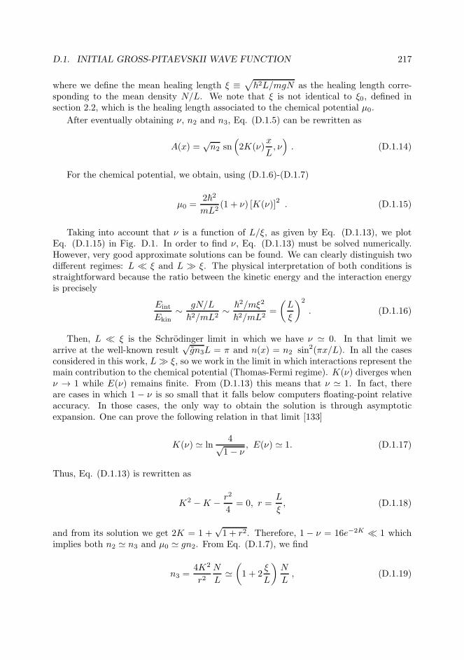
D.1. INITIAL GROSS-PITAEVSKII WAVE FUNCTION 217
where we define the mean healing length ξ ≡√
~2L/mgN as the healing length corre-sponding to the mean density N/L. We note that ξ is not identical to ξ0, defined insection 2.2, which is the healing length associated to the chemical potential µ0.
After eventually obtaining ν, n2 and n3, Eq. (D.1.5) can be rewritten as
A(x) =√n2 sn
(
2K(ν)x
L, ν)
. (D.1.14)
For the chemical potential, we obtain, using (D.1.6)-(D.1.7)
µ0 =2~2
mL2(1 + ν) [K(ν)]2 . (D.1.15)
Taking into account that ν is a function of L/ξ, as given by Eq. (D.1.13), we plotEq. (D.1.15) in Fig. D.1. In order to find ν, Eq. (D.1.13) must be solved numerically.However, very good approximate solutions can be found. We can clearly distinguish twodifferent regimes: L ≪ ξ and L ≫ ξ. The physical interpretation of both conditions isstraightforward because the ratio between the kinetic energy and the interaction energyis precisely
Eint
Ekin∼ gN/L
~2/mL2∼ ~2/mξ2
~2/mL2=
(
L
ξ
)2
. (D.1.16)
Then, L ≪ ξ is the Schrodinger limit in which we have ν ≃ 0. In that limit wearrive at the well-known result
√gn3L = π and n(x) = n2 sin2(πx/L). In all the cases
considered in this work, L≫ ξ, so we work in the limit in which interactions represent themain contribution to the chemical potential (Thomas-Fermi regime). K(ν) diverges whenν → 1 while E(ν) remains finite. From (D.1.13) this means that ν ≃ 1. In fact, thereare cases in which 1 − ν is so small that it falls below computers floating-point relativeaccuracy. In those cases, the only way to obtain the solution is through asymptoticexpansion. One can prove the following relation in that limit [133]
K(ν) ≃ ln4√1− ν
, E(ν) ≃ 1. (D.1.17)
Thus, Eq. (D.1.13) is rewritten as
K2 −K − r2
4= 0, r =
L
ξ, (D.1.18)
and from its solution we get 2K = 1 +√1 + r2. Therefore, 1 − ν = 16e−2K ≪ 1 which
implies both n2 ≃ n3 and µ0 ≃ gn2. From Eq. (D.1.7), we find
n3 =4K2
r2N
L≃(
1 + 2ξ
L
)
N
L, (D.1.19)
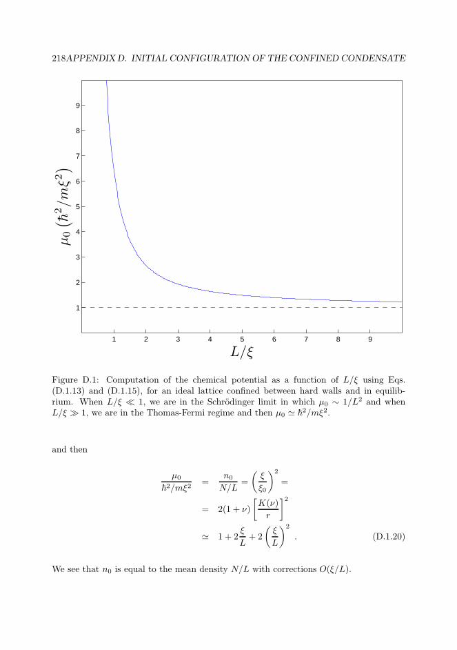
218APPENDIX D. INITIAL CONFIGURATION OF THE CONFINED CONDENSATE
1 2 3 4 5 6 7 8 9
1
2
3
4
5
6
7
8
9
L/ξ
µ0
(
h2/m
ξ2)
Figure D.1: Computation of the chemical potential as a function of L/ξ using Eqs.(D.1.13) and (D.1.15), for an ideal lattice confined between hard walls and in equilib-rium. When L/ξ ≪ 1, we are in the Schrodinger limit in which µ0 ∼ 1/L2 and whenL/ξ ≫ 1, we are in the Thomas-Fermi regime and then µ0 ≃ ~2/mξ2.
and then
µ0
~2/mξ2=
n0
N/L=
(
ξ
ξ0
)2
=
= 2(1 + ν)
[
K(ν)
r
]2
≃ 1 + 2ξ
L+ 2
(
ξ
L
)2
. (D.1.20)
We see that n0 is equal to the mean density N/L with corrections O(ξ/L).
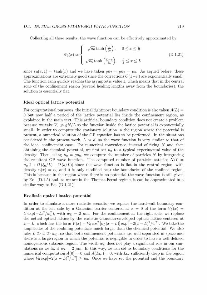
D.1. INITIAL GROSS-PITAEVSKII WAVE FUNCTION 219
Collecting all these results, the wave function can be effectively approximated by
Ψ0(x) ≃
√n0 tanh
(
xξ0
)
, 0 ≤ x ≤ L2
√n0 tanh
(
L−xξ0
)
, L2 ≤ x ≤ L
(D.1.21)
since sn(x, 1) = tanh(x) and we have taken gn2 = gn3 = µ0. As argued before, theseapproximations are extremely good since the corrections O(1−ν) are exponentially small.The function tanh quickly reaches the asymptotic value 1, which means that in the centralzone of the confinement region (several healing lengths away from the boundaries), thesolution is essentially flat.
Ideal optical lattice potential
For computational purposes, the initial rightmost boundary condition is also takenA(L) =0 but now half a period of the lattice potential lies inside the confinement region, asexplained in the main text. This artificial boundary condition does not create a problembecause we take V0 ≫ gN/L so the function inside the lattice potential is exponentiallysmall. In order to compute the stationary solution in the region where the potential ispresent, a numerical solution of the GP equation has to be performed. In the situationsconsidered in the present work, L ≫ d, so the wave function is very similar to that ofthe ideal confinement case. For numerical convenience, instead of fixing N and thenobtaining the chemical potential, we first set n0 to a typical experimental value of thedensity. Then, using µ0 = gn0, we compute the number of particles N by integratingthe resultant GP wave function. The computed number of particles satisfies N/L =n0 [1 +O (ξ0/L) +O (d/L)] since the wave function is flat in the central region, withdensity n(x) = n0 and it is only modified near the boundaries of the confined region.This is because in the region where there is no potential the wave function is still givenby Eq. (D.1.5) and, as we are in the Thomas-Fermi regime, it can be approximated in asimilar way to Eq. (D.1.21).
Realistic optical lattice potential
In order to simulate a more realistic scenario, we replace the hard-wall boundary con-dition at the left side by a Gaussian barrier centered at x = 0 of the form VL(x) =U exp(−2x2/w2
L), with wL = 2 µm. For the confinement at the right side, we replacethe actual optical lattice by the realistic Gaussian-enveloped optical lattice centered atx = L, which has the form V (x) = V0 cos
2 [kL(x− L)] exp[
−2(x− L)2/w2]
. We take theamplitudes of the confining potentials much larger than the chemical potential. We alsotake L ≫ w ≫ wL, so that both confinement potentials are well separated in space andthere is a large region in which the potential is negligible in order to have a well-definedhomogeneous subsonic region. The width wL does not play a significant role in our sim-ulations so we fix it wL = 2 µm. In this way, we can set as boundary conditions for thenumerical computation A(0) = 0 and A(Lbc) = 0, with Lbc sufficiently deep in the regionwhere V0 exp[−2(x − L)2/w2] ≥ µ0. Once we have set the potential and the boundary
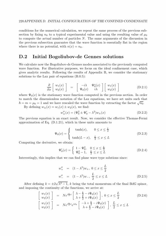
220APPENDIX D. INITIAL CONFIGURATION OF THE CONFINED CONDENSATE
conditions for the numerical calculation, we repeat the same process of the previous sub-section by fixing n0 to a typical experimental value and using the resulting value of µ0
to compute the actual number of particles N . The same arguments of the discussion inthe previous subsection guarantee that the wave function is essentially flat in the regionwhere there is no potential, with n(x) = n0.
D.2 Initial Bogoliubov-de Gennes solutions
We calculate now the Bogoliubov-de Gennes modes associated to the previously computedwave function. For illustrative purposes, we focus on the ideal confinement case, whichgives analytic results. Following the results of Appendix B, we consider the stationarysolutions to the Lax pair of equations (B.0.5):
∂
∂x
[
w1(x)w2(x)
]
=
[
−iλ Ψ∗0(x)
Ψ0(x) iλ
] [
w1(x)w2(x)
]
(D.2.1)
where Ψ0(x) is the stationary wave function computed in the previous section. In orderto match the dimensionless notation of the Lax equations, we have set units such that~ = m = µ0 = 1 and we have rescaled the wave function by extracting the factor
√n0.
By defining w±(x) = w1(x)± w2(x), we find:
w′′±(x) = (Ψ2
0 ±Ψ′0 − λ2)w±(x) (D.2.2)
The previous equation is an exact result. Now, we consider the effective Thomas-Fermiapproximation of Eq. (D.1.21), which in these units amounts to
Ψ0(x) =
tanh(x), 0 ≤ x ≤ L2
tanh(L− x), L2 ≤ x ≤ L
(D.2.3)
Computing the derivative, we obtain:
Ψ′0(x) =
1−Ψ20, 0 ≤ x ≤ L
2
Ψ20 − 1, L
2 ≤ x ≤ L(D.2.4)
Interestingly, this implies that we can find plane wave type solutions since:
w′′+ = (1 − λ2)w+, 0 ≤ x ≤ L
2
w′′− = (1 − λ2)w−,
L
2≤ x ≤ L (D.2.5)
After defining k = ±2√λ2 − 1, k being the total momentum of the final BdG spinor,
and imposing the continuity of the functions, we arrive at:[
w1(x)w2(x)
]
= Neik2 x
[
λ− k2 − iΨ0(x)
λ+ k2 + iΨ0(x)
]
, 0 ≤ x ≤ L
2(D.2.6)
[
w1(x)w2(x)
]
= Neik2 xeiφk
[
−λ+ k2 − iΨ0(x)
λ+ k2 − iΨ0(x)
]
,L
2≤ x ≤ L

D.2. INITIAL BOGOLIUBOV-DE GENNES SOLUTIONS 221
with φk = arctan 2/k and N some normalization constant. Using the temporal Laxequation of (B.0.5), we find ω = λk.
In the flat zone of the GP wave function, these plane wave solutions correspond to theusually considered BdG solutions for a condensate with zero momentum. For given ω, wehave 4 values of k that come in pairs (k,−k). One pair corresponds to plane wave typesolutions and the other pair to exponential type solutions. Now, we set the hard-wallboundary condition u(0) = v(0) = 0 which reduces the 4 independent solutions to 2.These new solutions are linear combinations of the (k,−k) pairs. Specifically, the realexponential type solutions give rise to:
[
u(x)v(x)
]
= C
(
(
ωκ − κ
2
)2+Ψ2
0(x))
sinh(κx) + 2Ψ0(x)(
ωκ − κ
2
)
cosh(κx)(
(
ωκ + κ
2
)2+Ψ2
0(x))
sinh(κx)− 2Ψ0(x)(
ωκ + κ
2
)
cosh(κx)
, 0 ≤ x ≤ L
2
[
u(x)v(x)
]
=
= C
(
(
ωκ − κ
2
)2+Ψ2
0(x))
sinh(κx+ uκ)− 2Ψ0(x)(
ωκ − κ
2
)
cosh(κx+ uκ)(
(
ωκ + κ
2
)2+Ψ2
0(x))
sinh(κx+ uκ) + 2Ψ0(x)(
ωκ + κ
2
)
cosh(κx+ uκ)
,L
2≤ x ≤ L
euκ =κ2 − 1κ2 + 1
(D.2.7)
while the stationary wave solution is:
[
u(x)v(x)
]
= C
(
(
ωk + k
2
)2 −Ψ20(x)
)
sin(kx) + 2Ψ0(x)(
ωk + k
2
)
cos(kx)(
(
ωk − k
2
)2 −Ψ20(x)
)
sin(kx)− 2Ψ0(x)(
ωk − k
2
)
cos(kx)
, 0 ≤ x ≤ L
2
[
u(x)v(x)
]
=
= C
(
(
ωk + k
2
)2 −Ψ20(x)
)
sin(kx+ 2φk)− 2Ψ0(x)(
ωk + k
2
)
cos(kx+ 2φk)(
(
ωk − k
2
)2 −Ψ20(x)
)
sin(kx+ 2φk) + 2Ψ0(x)(
ωk − k
2
)
cos(kx+ 2φk)
,L
2≤ x ≤ L
(D.2.8)
with C some normalization constant. We compute now the BdG solutions in the idealconfinement case. Using only the stationary wave solution and taking into account theother boundary condition u(L) = v(L) = 0, we find that the energies and the solutionsare quantized through:
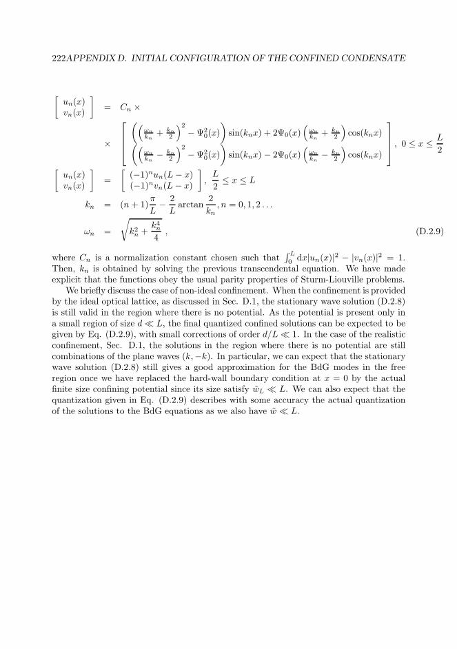
222APPENDIX D. INITIAL CONFIGURATION OF THE CONFINED CONDENSATE
[
un(x)vn(x)
]
= Cn ×
×
(
(
ωn
kn+ kn
2
)2
−Ψ20(x)
)
sin(knx) + 2Ψ0(x)(
ωn
kn+ kn
2
)
cos(knx)(
(
ωn
kn− kn
2
)2
−Ψ20(x)
)
sin(knx) − 2Ψ0(x)(
ωn
kn− kn
2
)
cos(knx)
, 0 ≤ x ≤ L
2
[
un(x)vn(x)
]
=
[
(−1)nun(L− x)(−1)nvn(L− x)
]
,L
2≤ x ≤ L
kn = (n+ 1)π
L− 2
Larctan
2
kn, n = 0, 1, 2 . . .
ωn =
√
k2n +k4n4, (D.2.9)
where Cn is a normalization constant chosen such that∫ L
0 dx|un(x)|2 − |vn(x)|2 = 1.Then, kn is obtained by solving the previous transcendental equation. We have madeexplicit that the functions obey the usual parity properties of Sturm-Liouville problems.
We briefly discuss the case of non-ideal confinement. When the confinement is providedby the ideal optical lattice, as discussed in Sec. D.1, the stationary wave solution (D.2.8)is still valid in the region where there is no potential. As the potential is present only ina small region of size d≪ L, the final quantized confined solutions can be expected to begiven by Eq. (D.2.9), with small corrections of order d/L≪ 1. In the case of the realisticconfinement, Sec. D.1, the solutions in the region where there is no potential are stillcombinations of the plane waves (k,−k). In particular, we can expect that the stationarywave solution (D.2.8) still gives a good approximation for the BdG modes in the freeregion once we have replaced the hard-wall boundary condition at x = 0 by the actualfinite size confining potential since its size satisfy wL ≪ L. We can also expect that thequantization given in Eq. (D.2.9) describes with some accuracy the actual quantizationof the solutions to the BdG equations as we also have w ≪ L.
Appendix EFlowing condensate in a nonlinear
optical lattice
E.1 General discussion
We review here the theory of a condensate in an optical lattice. Most of the results areextracted from Ref. [50]. The time-independent GP equation in an ideal infinite opticallattice whose potential has the same form of the long-time potential of Eq. (2.2.3),V (x) = V∞ cos2(kLx), reads
− ~2
2m
d2Ψ0
dx2+ V∞ cos2(kLx)Ψ0(x) + g|Ψ0(x)|2Ψ0 = µΨ0 (E.1.1)
For simplifying the calculations, we define the dimensionless length z ≡ 2kLx and rescalethe wave function as Ψ0 → √
nrΨ0, with nr the average atomic density, so it becomedimensionless. Using these quantities, we can rewrite the GP equation as:
− 1
2
d2Ψ0
dz2+ v cos(z)Ψ0 + c2|Ψ0(z)|2Ψ0 = αΨ0 (E.1.2)
with
v =V∞2EL
, c2 =gnr
EL, α =
µ− V∞/2
EL, EL =
4~2k2Lm
= 8ER (E.1.3)
Here, α is the dimensionless chemical potential, displaced −V∞/2, and c is the dimen-sionless speed of sound of the lattice in the limit of vanishing amplitude v → 0.
We look for Bloch type solutions of the form
Ψ0(z) = eiqzyq(z), (E.1.4)
with yq(z + 2π) = yq(z) periodic since the non-linear term is periodic for a Bloch-wavetype solution. The normalization condition reads now
1
2π
∫ 2π
0
dz |Ψ0(z)|2 =1
2π
∫ 2π
0
dz |yq(z)|2 = 1. (E.1.5)
223

224APPENDIX E. FLOWINGCONDENSATE IN A NONLINEAROPTICAL LATTICE
The Brillouin zone is placed in the region −1/2 < q < 1/2. The equation for yq reads:
− 1
2
(
∂
∂z+ iq
)2
yq + v cos(z)yq + c2|yq|2yq = αqyq, (E.1.6)
where we have allowed for a q - dependence of α. The linear Schrodinger regime is obtainedwhen c = 0. For c2 > v, some extra non-linear Bloch waves appear. This generates aloop structure in the conduction band. In the systems analyzed in the present work,c2 ∼ 10−3 − 10−4 and v ∼ 10−1, hence v ≫ c2. As a consequence: (a) loops do notappear; (b) the system is close to the linear Schrodinger regime.
To compute the Bloch energy eigenvalues, we follow the method developed in Ref.[50]. First, we perform a finite Fourier expansion of the periodic function yq(z) of theform:
yq(z) =M∑
n=−M
cneinz , (E.1.7)
where M is a numerically enforced cut-off. After substitution of this solution in (E.1.6)and in (E.1.5), we get 2M + 2 equations for 2M + 2 variables (the 2M + 1 values of theFourier coefficients cn plus the eigenvalue α). Instead of directly solving these non-linearequations, it is more efficient to minimize the quadratic sum of the 2M + 2 equations,
S =
2M+2∑
j=1
f2j , (E.1.8)
where fj(cn, α) = 0 (with j = 1, 2 . . . 2M +2) are the equations to be solved. It is easy tosee that all these equations are real, so the coefficients cn can be chosen as real numbersand there is no need to take the modulus in Eq. (E.1.8).
A given Bloch solution can be unstable, either dynamically or in the sense of Landau,as explained in Sec. 1.2.1. We rewrite the functional (1.2.18) in our system of units as:
K [Ψ] =
∫
dz
[
1
2
∣
∣
∣
∣
∂Ψ
∂z
∣
∣
∣
∣
2
+ v cos(z)|Ψ|2 + c2
2|Ψ|4 − α|Ψ|2
]
. (E.1.9)
Considering linear perturbations around the stationary solution Ψ0 as in Eq. (1.2.19), wefind:
δK =1
2
∫
dz [δΨ∗ δΨ]Λ
[
δΨδΨ∗
]
Λ =
[
H ′ LL∗ H ′
]
H ′ = −1
2
∂2
∂z2+ v cos(z) + 2c2|Ψ0|2 − αq
L = c2Ψ20 . (E.1.10)

E.1. GENERAL DISCUSSION 225
The appearance of negative eigenvalues in the Hermitian operator Λ indicates that thewave function is energetically unstable. The corresponding eigenvalue equation reads
Λ
[
uv
]
= λ
[
uv
]
. (E.1.11)
By absorbing the exponential plane-wave factor of the Bloch-type GP solution, u(z) =eiqzuq(z) and v(z) = e−iqzvq(z), we arrive at a new matrix operator Λq which is periodic.
Applying Bloch’s theorem in the form uq(z) = eikzuq,k(z) and vq(z) = eikzvq,k(z) withuq,k(z) and vq,k(z) periodic in [0, 2π], the final eigenvalue equation reads
Λq,k
[
uq,kvq,k
]
= λq,k
[
uq,kvq,k
]
Λq,k =
[
H′′
k+qLq
L∗q H
′′
k−q
]
H′′
k= −1
2
(
∂
∂z+ ik
)2
+ v cos(z) + 2c2|yq|2 − α
Lq = c2y2q . (E.1.12)
Dynamical instabilities correspond to modes that grow exponentially with time. Theyare computed by looking for non-real eigenvalues of the BdG equations, formally similarto Eq. (E.1.11):
M
[
uv
]
= ǫ
[
uv
]
, (E.1.13)
with M = σzΛ and ǫ is the dimensionless energy (in units of EL). Bloch’s theorem alsoapplies here and after a computation similar to that which has led to Eq. (E.1.12), theeigenvalue equation reads
Mq,k
[
uq,kvq,k
]
= ǫq,k
[
uq,kvq,k
]
, (E.1.14)
with Mq,k = σzΛq,k. As shown in the main text, the system can only be dynamicallyunstable whenever it is already Landau unstable. A plot of the parameter regions wherethe system is Landau and dynamically unstable can be found in Ref. [50].
In addition to the dynamical stability analysis, the real eigenvalues of this operator canbe used to compute the speed of sound in the optical lattice. When q = 0, it can be proventhat for small (dimensionless) wave-vector k, the eigenvalues go like ǫ = ±s|k|, with s thedimensionless speed of sound (here, in units of 2~kL/m). On the other hand, the form ofthe Bloch-type solution of the GP equation as a function of both Bloch momentum anddensity can be directly used to compute the sound speed without the need to solve forthe BdG equations [27]. Restoring dimensions with q = 2kLq, the sound speed s in thelattice is
s =
√
∂2nE∂2qE~
(E.1.15)

226APPENDIX E. FLOWINGCONDENSATE IN A NONLINEAROPTICAL LATTICE
where ∂n denotes derivative with respect the mean density, nr, ∂q is the derivative withrespect the Bloch momentum q, with both derivatives evaluated at q = 0. In the previousexpression, E is the average energy density, given by
E =nr
d
∫ d
0
dx y∗q (x)
[
− ~2
2m
(
∂
∂x+ iq
)2
+ V∞ cos2(kLx) +gnr
2|yq(x)|2
]
yq(x)
= nrµ− gn2r
4π
∫ 2π
0
dz |yq(z)|4. (E.1.16)
E.2 Perturbative treatment
We consider now a perturbative treatment of the results presented in the previous sec-tion. In Eq. (E.1.2) there are two dimensionless parameters, v and c2. The former isessentially the amplitude of the potential (v ≫ 1 is the tight-binding regime while v ≪ 1corresponds the nearly-free-particle regime) and the latter is a measure of the strength ofthe interaction or nonlinearity. In the cases studied in this work, v ≪ 1 but the followingdiscussion applies to arbitrary values of v. The quantity δ ≡ c2 ≪ 1 is the small parame-ter of our perturbation theory. We expand in powers of δ both the Bloch wave yq(z) andthe displaced and dimensionless chemical potential αq, which solve Eqs. (E.1.5)-(E.1.6).We obtain
yq(z) =
∞∑
n=0
δny(n)q (z) ,
αq =
∞∑
n=0
δnα(n)q , (E.2.1)
which transforms Eq. (E.1.6) into
H(0)q yq + δ|yq|2yq = αqyq
H(0)q ≡ −1
2
(
∂
∂z+ iq
)2
+ v cos(z) . (E.2.2)
In the following, we focus on the lowest Bloch band and keep terms up to O(δ2). The
lowest-order term solves the linear Schrodinger equation, H(0)q y
(0)q = α
(0)q y
(0)q . Therefore,
y(0)q = φq,0 and α
(0)q = εq,0, where φq,0(z) is the corresponding eigenfunction for the lowest
band, which involves Mathieu functions, and εq,0 its dimensionless eigenvalue (note theuse of the index 0 for two different purposes: perturbative order in the superindex andband index in the subindex). φq,0 is normalized according to Eq. (E.1.5).
The first-order corrections satisfy
H(0)q y
(1)q + |y(0)q |2y(0)q = α
(0)q y
(1)q + α
(1)q y
(0)q , (E.2.3)

E.2. PERTURBATIVE TREATMENT 227
which, using standard perturbation techniques, leads to
α(1)q =
1
2π
∫ 2π
0
dz|φq,0|4
y(1)q =
∞∑
n=1
βnφq,n
βn =12π
∫ 2π
0dz φ∗q,n|φq,0|2φq,0εq,0 − εq,n
, (E.2.4)
where φq,n∞n=1 are the Schrodinger eigenvectors of the rest of bands and εq,n its corre-sponding eigenvalues, for a given value of q.
The second-order equation reads
H(0)q y
(2)q + 2|y(0)q |2y(1)q + y
(0)2q y
(1)∗q = α
(0)q y
(2)q + α
(1)q y
(1)q + α
(2)q y
(0)q . (E.2.5)
We note that y(2)q is not needed to compute α
(2)q . Specifically,
α(2)q =
1
2π
∫ 2π
0
dz|φq,0|2(2φ∗q,0y(1)q + φq,0y
(1)∗q ) = −3
∞∑
n=1
|βn|2(εq,n − εq,0), (E.2.6)
which is always negative.Instead of invoking Mathieu functions and integrals of them, the numerical compu-
tation of the formulae presented in this Appendix [Eqs. (E.2.4), (E.2.6)] can be easilyperformed in a Fourier representation. As yq, φq,n are periodic functions in [0, 2π], theirFourier expansion read yq(z) =
∑∞m=−∞ cme
imz and φq,n(z) =∑∞
m=−∞ an,meimz. Both
the cm and the an,m coefficients can be chosen real [see discussion after Eq. (E.1.8)]. In
this Fourier representation, H(0)q is a tridiagonal matrix with elements Hm,m±1 = v/2
and Hm,m = (m + q)2/2. Multiplication by |φq,0|2 is represented by the matrix rm,p =∑
l a0,la0,l+m−p. The perturbative expansion of the Fourier components of solution to
the GP equation reads cm =∑∞
n=0 δnc
(n)m . In this Fourier basis, the Schrodinger equation
for all the bands is written as an eigenvalue-eigenvector matrix equation
Han = εq,nan, (E.2.7)
where matrix multiplication is understood. We can also rewrite Eqs. (E.2.4), (E.2.6) as:
α(1)q = aT0 ra0
c(1) =
∞∑
n=1
βnan
βn =aTnra0
εq,0 − εq,n
α(2)q = 3aT0 rc
(1) = −3
∞∑
n=1
|βn|2(εq,n − εq,0). (E.2.8)

228APPENDIX E. FLOWINGCONDENSATE IN A NONLINEAROPTICAL LATTICE
In practice, we impose a numerical cut-off in the Fourier series as that of Eq. (E.1.7) tocompute the previous magnitudes. Now we can use the previous perturbative results togive approximate closed expressions for some magnitudes of the optical lattice. To firstorder in δ, the energy density is given by Eq. (E.1.16)
E ≃ nr
(
µ− gnr
2α(1)q
)
. (E.2.9)
We can write
µ = ELα+V∞2
≃ ELα(0)q +
V∞2
+ ELα(1)q δ = µ(0) + ELα
(1)q δ (E.2.10)
On the other hand, for the non-interacting chemical potential we have (assuming q ≪1/2):
µ(0) = µ(0)(q) ≃ Emin +~2q2
2m∗ , (E.2.11)
where Emin is the bottom of the Schrodinger conduction band as defined in the main text,m∗ is the effective mass, and we recall q = 2kLq. Thus,
µ = Emin +~2q2
2m∗ + gnrα(1)q . (E.2.12)
Using (E.2.12) we can rewrite (E.2.9) as
E ≃ nrEmin + nr~2q2
2m∗ +gn2
r
2α(1)q . (E.2.13)
Computing the derivatives of Eq. (E.1.15) to lowest order in δ, we obtain:
(
∂2E∂q2
)
q=0
≃ nr~2
m∗ ,
(
∂2E∂n2
r
)
q=0
≃ gα(1)0 . (E.2.14)
and the speed of sound then reads
s =
√
gnr
m∗ α(1)0 =
√
gnr
m
√
m
m∗α(1)0 . (E.2.15)
Similar results appear in Ref. [138] and references therein. The first square root is thespeed of sound in the absence of the optical lattice. The second factor on the righttakes into account the presence of the optical lattice and is practically unity for v ≪ 1.Specifically, we can write:
m∗ = m[
1 + 8v2 +O(v4)]
α(1)q = 1 +
8v2
(1 − 4q2)2+O(v4), (E.2.16)
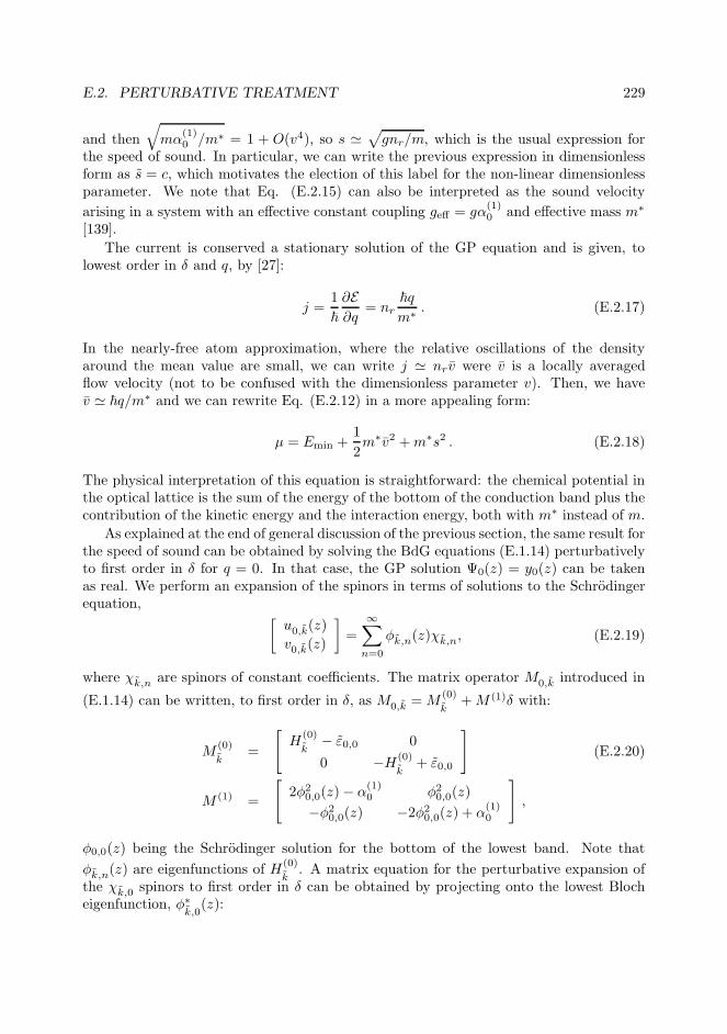
E.2. PERTURBATIVE TREATMENT 229
and then
√
mα(1)0 /m∗ = 1 + O(v4), so s ≃
√
gnr/m, which is the usual expression forthe speed of sound. In particular, we can write the previous expression in dimensionlessform as s = c, which motivates the election of this label for the non-linear dimensionlessparameter. We note that Eq. (E.2.15) can also be interpreted as the sound velocity
arising in a system with an effective constant coupling geff = gα(1)0 and effective mass m∗
[139].
The current is conserved a stationary solution of the GP equation and is given, tolowest order in δ and q, by [27]:
j =1
~
∂E∂q
= nr~q
m∗ . (E.2.17)
In the nearly-free atom approximation, where the relative oscillations of the densityaround the mean value are small, we can write j ≃ nrv were v is a locally averagedflow velocity (not to be confused with the dimensionless parameter v). Then, we havev ≃ ~q/m∗ and we can rewrite Eq. (E.2.12) in a more appealing form:
µ = Emin +1
2m∗v2 +m∗s2 . (E.2.18)
The physical interpretation of this equation is straightforward: the chemical potential inthe optical lattice is the sum of the energy of the bottom of the conduction band plus thecontribution of the kinetic energy and the interaction energy, both with m∗ instead of m.
As explained at the end of general discussion of the previous section, the same result forthe speed of sound can be obtained by solving the BdG equations (E.1.14) perturbativelyto first order in δ for q = 0. In that case, the GP solution Ψ0(z) = y0(z) can be takenas real. We perform an expansion of the spinors in terms of solutions to the Schrodingerequation,
[
u0,k(z)
v0,k(z)
]
=
∞∑
n=0
φk,n(z)χk,n, (E.2.19)
where χk,n are spinors of constant coefficients. The matrix operator M0,k introduced in
(E.1.14) can be written, to first order in δ, as M0,k =M(0)
k+M (1)δ with:
M(0)
k=
[
H(0)
k− ε0,0 0
0 −H(0)
k+ ε0,0
]
(E.2.20)
M (1) =
[
2φ20,0(z)− α(1)0 φ20,0(z)
−φ20,0(z) −2φ20,0(z) + α(1)0
]
,
φ0,0(z) being the Schrodinger solution for the bottom of the lowest band. Note that
φk,n(z) are eigenfunctions of H(0)
k. A matrix equation for the perturbative expansion of
the χk,0 spinors to first order in δ can be obtained by projecting onto the lowest Blocheigenfunction, φ∗
k,0(z):

230APPENDIX E. FLOWINGCONDENSATE IN A NONLINEAROPTICAL LATTICE
ǫ(q = 0, k)χk,0 =
[
εk,0 − ε0,0 + (2J(k)− α(1)0 )δ J(k)δ
−J(k)δ −εk,0 + ε0,0 − (2J(k)− α(1)0 )δ
]
χk,0
J(k) =1
2π
∫ 2π
0
dz|φk,0|2|φ0,0|2. (E.2.21)
Restoring units for k by using k = 2kLk, expanding to lowest order near k = 0, andneglecting corrections O(δ) to m∗, the eigenvalues are approximated as
ǫ(0, k) = ±[
(
~2k2
2m∗
)2
+ gnrα(1)0
~2k2
m∗
]12
, (E.2.22)
which for small k gives ǫ(0, k) ≃ ~sk with s given by (E.2.15). As the optical lattice issubsonic, for given ǫ, apart from the two solutions with (k,−k), we have another twosolutions with complex wave vector, similar to the subsonic region of a black-hole.
The previous results can be used to compute the corrections to the width of the lowestband, which by virtue of Eq. (E.2.21) give
∆BdGc ≃ ∆c +
[
2J(1/2)− α(1)0
]
gnr , (E.2.23)
where ∆c = EL(ε 12 ,0
− ε0,0) is the Schrodinger bandwidth and we have used ∆c ≫ gnr,which is true in all the situations considered in the present work. We see that in the limitof negligible interactions, the BdG bandwidth is equal to the linear bandwidth.

Appendix FNumerical methods
Several numerical methods have been used across the work to integrate both the GP andBdG equations. We now explain in detail those numerical schemes.
F.1 Birth of a black hole in an optical lattice
In Chapter 2, we integrate the time-dependent GP equation (2.2.1) to obtain the timeevolution of the system. After that, once in the quasi-stationary regime, we solve theresulting effective time-independent BdG equations in order to obtain the Hawking spec-trum of the formed black-hole.
F.1.1 Time-dependent GP equation
Crank-Nicolson method
The numerical computation of the time evolution of the GP wave function has beenperformed using the Crank-Nicolson method, as in Ref. [39]. The spatial interval [0, Lg]is divided into N + 2 equally spaced points separated by a distance ∆x = Lg/(N + 1),and the time interval [0, t] into steps of size ∆t. Hence, we write the grid points as
xj = j∆x j = 0, 1 . . .N + 1
tk = k∆t k = 0, 1 . . . n . (F.1.1)
For computational purposes, we work with a dimensionless GP equation so we set unitssuch that ~ = m = ξ0 = 1, and rescale the wave function by extracting the factor
√n0.
The GP equation can be then written as
i∂Ψ(x, t)
∂t= H(x, t)Ψ(x, t) (F.1.2)
H(x, t) = −1
2
∂2
∂x2+ V (x, t) + |Ψ(x, t)|2 − 1
231

232 APPENDIX F. NUMERICAL METHODS
where the ”−1” comes from subtracting the initial chemical potential µ0 and V (x, t) isthe total external time-dependent potential. Here, H(x, t) plays the role of an effectiveHamiltonian. If we define the spatial vector with the discrete values of the wave functionat a given time tk as Ψk, with components Ψj
k = Ψ(xj , tk), and using
Ψ
(
x, t+∆t
2
)
=Ψ(x, t+∆t) + Ψ(x, t)
2+O
(
∆t2)
∂Ψ
∂t
(
x, t+∆t
2
)
=Ψ(x, t+∆t)−Ψ(x, t)
∆t+O
(
∆t2)
(F.1.3)
∂2Ψ
∂x2(x, t) =
Ψ (x+∆x, t) + Ψ (x−∆x, t) − 2Ψ(x, t)
∆x2+O
(
∆x2)
,
we can write, up to second order in ∆x and ∆t, a discrete version of Eq. (F.1.2)
iΨk+1 −Ψk
∆t= Hk+ 1
2
Ψk+1 +Ψk
2(
Hk+ 12Ψ)j
= −Ψj+1 +Ψj−1 − 2Ψj
2(∆x)2+ V j
k+ 12
Ψj + |Ψj
k+ 12
|2Ψj −Ψj
V j
k+ 12
= V
(
xj , tk +∆t
2
)
. (F.1.4)
The previous equation can be rewritten as a linear system of equations:
M2Ψk+1 = M1Ψk
M1,2 = 1∓ iHk+ 12
∆t
2, (F.1.5)
where
M1,2 =
. . .. . .
. . .
±A 1∓Bjk ±A
±A 1∓Bj+1k ±A
. . .. . .
. . .
, (F.1.6)
with
A =i∆t
4∆x2, Bj
k = i∆t
2
(
1
∆x2+ V j
k+ 12
+ |Ψj
k+ 12
|2 − 1
)
. (F.1.7)
The previous method is equivalent to approximate the time evolution operator between tand t+∆t by its Cayley’s form [140], given by the unitary operator:
U(t+∆t, t) ≃[
1 + iH
(
x, t+∆t
2
)
∆t
2
]−1 [
1− iH
(
x, t+∆t
2
)
∆t
2
]
(F.1.8)
Because we ignore the value of Ψj
k+ 12
in the non-linear term, we use a corrector-predictor
method, which consists in performing an additional step in every time iteration. In the

F.1. BIRTH OF A BLACK HOLE IN AN OPTICAL LATTICE 233
first iteration, we use Ψjk instead of Ψj
k+ 12
in order to obtain a value Ψjk+1. Next, we
perform a new iteration taking Ψj
k+ 12
=(
Ψjk+1 +Ψj
k
)
/2 to obtain the final value Ψjk+1.
The main advantage of this integration scheme is that the obtention of Ψjk+1 only
requires the resolution of a tridiagonal system of equations, which is computationallyvery efficient when using the Thomas algorithm [141, 142] to solve it, since in that casethe number of operations grows like N . Another important advantage of using the Crank-Nicolson method is that it is unconditionally unstable and then we can take higher valuesof ∆x,∆t than usual.
Absorbing boundary conditions
We now discuss the implementation of the boundary conditions, which affect to the firstand last points of the numerical grid. For instance, periodic boundary conditions aregiven by:
Ψ0k = ΨN+1
k , l = 0, N + 1, (F.1.9)
so the point N + 1 is identified with the point 0 and does not play any role on thedynamics. The periodic boundary conditions are simply implemented by writing the firstand last rows of the M matrices in Eq. (F.1.6) as:
M1,2 =
1∓B0k ±A . . . ±A
. . .. . .
±A . . . ±A 1∓BNk
, (F.1.10)
so the M matrices are (N +1)× (N +1). More relevant boundary conditions for our caseare the so-called hard-wall boundary conditions, expressed by the condition
Ψlk = 0, l = 0, N + 1, (F.1.11)
These boundary conditions are easily implemented by suppressing the first and the lastcolumns of the M matrices in Eq. (F.1.6), arriving to N ×N matrices of the form:
M1,2 =
1∓B1k ±A
. . .. . .
±A 1∓BNk
(F.1.12)
As explained in the main text, we implement a hard-wall boundary condition at x = 0 inorder to simulate the confinement of the potential. Even in the realistic case of Sec. 2.5,where the left confinement is provided by a finite barrier, this boundary condition is setto truncate the otherwise infinite numerical grid. As explained in Sec. D.1, this does notpose any problem since the amplitude of the confining potential is taken sufficiently largeso the condensate has exponentially small amplitude within the barrier.
On the other hand, imposing any of the previous boundary conditions at the finalpoint of the grid (x = Lg) will induce unwanted reflections because our goal is to simulatea semi-infinite supersonic region. To minimize those spurious reflections, one can use

234 APPENDIX F. NUMERICAL METHODS
complex absorbing potentials (CAP) at the grid boundaries [143]. Other possible methodcould be the implementation of a diffusive scheme near the boundaries of the grid; weuse this method for integrating the GP equation corresponding to the BH laser scenarioof Chapter 4, see Sec. F.2. Instead of those methods, we make use of the so-called ABC(Absorbing Boundary Conditions) [144, 145]. The ABC are based on the linearization ofthe dispersion relation at the boundary in order to achieve the relation corresponding toan outgoing plane wave. All the above mentioned methods are very useful because theynot only prevent the artificial reflection of the waves but also permit to reduce the size ofthe supersonic zone.
The point x = Lg is placed in the supersonic zone, where there is no potential. Inaddition, we expect that the non-linear term in Eq. (F.1.2) is sufficiently small to beneglected. This means that the effective Hamiltonian H in this region is the usual free(Schrodinger) Hamiltonian and Eq. (F.1.2) can be written as
i∂Ψ
∂t= −1
2
∂2Ψ
∂x2−Ψ (F.1.13)
which implies the dispersion relation
ω =k2
2− 1 (F.1.14)
On the supersonic side and in the quasi-stationary regime, the wave function is wellpeaked in momentum space around a value k0 ≃
√2Emin, where Emin is the energy of
the bottom of the first conduction band. By linearizing the dispersion relation around k0and expressing this relation in terms of derivatives, one gets
i∂Ψ
∂t= −ik0
∂Ψ
∂x−(
k202
+ 1
)
Ψ . (F.1.15)
We replace the hard-wall boundary condition at j = N + 1, Eq. (F.1.11), by the discreteversion of Eq. (F.1.15) at j = N . Then there are N+1 variables (Ψj
k, j = 1 . . . N+1) andN +1 equations, corresponding to N equations resulting from Eq. (F.1.4) for j = 1 . . .Nand the ABC equation. We can regard the point xN+1 as a ghost point because theGP equation is not properly defined there and the ABC (F.1.15) is the correspondingequation for this point [145]. Following these considerations, we can easily implement theABC condition by adding a new row to the matrices M of Eq. (F.1.12), which now areof size (N + 1)× (N + 1) and of the form
M1,2 =
. . .. . .
±A 1∓BNk ±A
±C 1±D ∓C
(F.1.16)
with
C =k0∆t
4∆x, D = i
∆t
2
(
k202
+ 1
)
(F.1.17)
Due to the finite size of the grid and to the nonzero width of the momentum distribu-tion in the supersonic region, the absorption is not perfect. Nevertheless, we have foundthat, in practice, the small spurious reflections have no effect on the final results.

F.1. BIRTH OF A BLACK HOLE IN AN OPTICAL LATTICE 235
F.1.2 Numerical integration of the quasi-stationary BdG equa-
tions
In order to obtain the scattering matrix in the quasi-stationary regime, we need to solvethe system of equations (C.1.6). The numerical computation of the fundamental matrixF (x) presents some problems in the optical lattice as one of the eigenvalues of the funda-mental matrix is exponentially large, corresponding to one of the local Bloch wave solu-tions with complex wave vector (see discussion at the end of Appendix E). For sufficientlylarge optical lattices, this makes that the fundamental matrix becomes singular withincomputer’s relative accuracy, spoiling the calculation. In order to deal with this problem,we consider two methods: QR decomposition [59] and the Global Matrix method [58].Both methods are based on the following property of the transfer matrix of Eq. (C.1.7):
T (xn+1, x1) =
n∏
i=1
Ti, Ti ≡ T (xi+1, xi) (F.1.18)
with x1 < x2 < . . . < xn+1, i.e., the total transfer matrix can be decomposed as theproduct of intermediate transfer matrices. In our problem, we have to compute thetransfer matrix T (xd, xu) between the two asymptotic regions so x1 = xu and xn+1 = xd.The two techniques here considered try to compute the previous product without finallyarriving at a numerical singular matrix. The matrices Ti are obtained by integratingthe effective BdG equations (2.6.3) on top of the quasi-stationary GP wave functionbetween the intermediate points xi and xi+1. The distance between consecutive pointsxi+1 − xi cannot be taken very large since in that case the local transfer matrices Ti alsobecome numerically singular. For the integration of the BdG equations, we use a Runge-Kutta method of fourth-order where the numerical grid is chosen such it coincides withthe numerical grid corresponding to the quasi-stationary GP wave function previouslycomputed.
We have checked that both methods work correctly by comparing the results with thebrute force result, in which the total transfer matrix is computed by direct multiplicationof Eq. (F.1.18) after increasing the accuracy to 1000 digits. Of course, brute forcerepresents a much slower method than the chosen methods, motivating their use. Wehave also checked the accuracy of the previous methods to obtain the scattering matrixby confirming the smallness of the elements of the residual matrix ∆η ≡ S†ηS− η, whichmeasures the pseudo-unitarity of the S matrix. Finally, we wish to note that there areno significant differences in the computational speed of both techniques so they representgood choices to do the job.
QR decomposition
As well known from linear algebra, a given matrix M can be decomposed as M = QRwith Q orthogonal and R an upper-diagonal matrix. This is called the QR decomposition.The point is that we can perform the QR decomposition at every step of the product ofEq. (F.1.18) in order to compute the QR decomposition of the total transfer matrix. IfT (xk, x1) = QkRk, with k < n + 1, we have T (xk+1, x1) = Tk+1T (xk, x1) = Tk+1QkRk
and we can obtain the QR decomposition of T (xk+1, x1) = Qk+1Rk+1 from the following

236 APPENDIX F. NUMERICAL METHODS
QR decomposition Tk+1Qk = QkRk, which gives Qk+1 = Qk and Rk+1 = RkRk. We canstart this recursive process from k = 2 until reaching k = n.
Once we get the Q,R matrices of the global transfer matrix, T (xd, xu) = QR, wecan compute the fundamental matrix in the supersonic region from that of the subsonicregion as F (xd) = QRF (xu). If we directly multiply QR we would get a singular matrix;instead of that, we first diagonalize the R matrix R = MDM−1 with D a diagonalmatrix (this diagonalization does not present any associated numerical problem since Ris an upper-diagonal matrix). As Q is orthogonal, detR = detD = 1. The matrix D hastwo eigenvalues that are exponentially large (small), which we denote as λ+,− (associatedto the complex Bloch wave vectors) and other two eigenvalues of order ∼ 1 (associatedto the propagating Bloch wave vectors). The numerical problem arises from mixing thecolumns of D, since λ+ crushes the eigenvalues of order 1 as they are so relatively smallthat they fall under computers relative accuracy.
For fixing this numerical issue, we first rearrange D so the column corresponding toλ+ is the first one. We then choose F (xu) such F (xu) = MI+, where I+ is the 4 × 4identity but with the first diagonal element replaced by λ−1
+ . As a consequence, we obtain
F (xd) = QMD where the matrix D is the same as D but with the first diagonal elementreplaced by 1. We note that, in this form, the columns of F (xu,d) are not mixed andthe Wronskian is conserved so the possible singular behavior disappears. However, forextremely long optical lattices, a problem of overflow can appear due to the exponentiallylarge value of λ+. In that limit case, there is no problem since we make use of the GlobalMatrix method.
Global Matrix method
The previous method just rearranges the product of Eq. (F.1.18) in a clever way in orderto obtain a non-singular matrix. This method avoids the explicit computation of the totaltransfer matrix; instead of that, we simply rewrite Eq. (C.1.6) as a (4n + 4) × (4n + 4)system of equations by also considering the matching of the solutions at the intermediatepoints x = xi, i = 2, 3, . . . , n
d = A · bb = [bu−out, bev, b1, b2, . . . , b4n−1, b4n, bd1−out, bd2−out]
T (F.1.19)
d = bu−in
σu−in,ω (xu)0...0
+ bd1−in
0...0
σd1−in,ω (xd)
+ bd2−in
0...0
σd2−in,ω (xd)
,
A =
−σu−out,ω −σev,ω I 0 0 . . . 0 00 0 T1 −I 0 . . . 0 00 0 0 T2 −I 0 . . . 0
. . .. . .
. . .
0 0 0 0 Tn−1 −I 0 00 0 0 0 0 Tn −σd1−out,ω −σd2−out,ω
F.2. TIME EVOLUTION OF THE BLACK-HOLE LASER 237
where the spatial dependence of the vectors σ inside the matrix A is understood. Inthis way, we prevent the appearance of singular behavior in the total transfer matrix bysolving at one time the global problem.
F.2 Time evolution of the black-hole laser
We discuss here the numerical method used to integrate the time dependent GP equation(4.3.1) which consists of a time-splitting finite-difference (TSFD) scheme [146, 147]. Westart by rewriting the corresponding GP equation as:
i∂Ψ(x, t)
∂t= H(x, t)Ψ(x, t)
= [H0(x, t) +HC(x, t)] Ψ(x, t) (F.2.1)
where H0 is the kinetic term and HC = g(x)(|Ψ(x, t)|2 − 1) is the term associated withthe contact interaction. We divide the spatial interval [−Lg/2, Lg/2] in N + 1 steps ofsize ∆x = Lg/(N + 1) and impose periodic boundary conditions. The time interval [0, t]is divided in n steps of size ∆t = t/n. Within this scheme, the (non-linear) time evolutionoperator from tk = k∆t to tk+1 = (k+1)∆t is computed using a split-step approximation
Uk ≃ e−iH0∆t2 e−iHk
C∆te−iH0∆t2 (F.2.2)
where HkC = g(x)(|Ψ(x, tk)|2 − 1), Ψ(x, tk) = e−iH0
∆t2 Ψ(x, tk). We refer to Sec. 5.5.1 for
a detailed theoretical discussion on the split-step method. The total evolution operatorthen reads
Ψ(x, t) = U(t)Ψ(x, 0) (F.2.3)
U(t) = e−iH0∆t2 e−iHn−1
C ∆t
(
n−2∏
k=0
e−iH0∆te−iHkC∆t
)
e−iH0∆t2
In the TSFD, instead of using the usual Fourier transform to compute the kineticevolution operator e−iH0∆t, we use the Crank-Nicolson method discussed in Sec. F.1.1.The corresponding Cayley’s form [see Eq. (F.1.8] is:
e−iH0∆t ≃(
1 + iH0∆t
2
)−1(
1− iH0∆t
2
)
(F.2.4)
When the previous operator acts on a given wave function Ψ, we obtain a new wavefunction Ψ′ = e−iH0∆tΨ. In order to compute Ψ′, we rewrite the previous equation inthe same implicit form of Eq. (F.1.5):
M2Ψ′ = M1Ψ
′
M1,2 = 1∓ iH0∆t
2, (F.2.5)
238 APPENDIX F. NUMERICAL METHODS
Ψ,Ψ′ being the spatial vectors with the discrete values of the wave functions Ψ,Ψ′ andH0 the discrete matrix corresponding to the kinetic operator. Following the results ofSec. F.1.1, we find:
M1,2 =
1∓ 2A ±A . . . . . . ±A±A 1∓ 2A ±A
. . .. . .
. . .
±A 1∓ 2A ±A±A . . . . . . ±A 1∓ 2A
, (F.2.6)
where we have taken into account that we are working with periodic boundary conditions,see Eq. (F.1.10). As explained in Sec. F.1.1, the Crank-Nicolson method is uncondition-ally unstable and very cheap from the computational point of view. Importantly, wenote that the matrix HD is constant in time, so we can develop an optimized Thomasalgorithm for the associated Crank-Nicolson scheme. In particular, the specific Thomasalgorithm developed in this work is able to defeat the standard linear solver of MATLAB!Another advantage is that this scheme keeps working even when the kinetic term involvesderivatives with a spatially dependent coefficient, see the discussion below.
Since we are focusing on long time dynamics, we add a diffusive term at the boundariesof the system in order to absorb the emitted waves and solitons so they do not return tothe central supersonic region and disturb the analysis of the simulations. Specifically, wereplace H by HT = H + iHA in Eq. (F.2.1), where the absorbing term HA is given by
HA(x, t) = G(x)(
D0∂2xe
−ivx − F0[|Ψ(x, t)|2 − 1])
. (F.2.7)
The function G(x) is a function localized on the boundary of the grid (typically a Gaussiandistribution) and it is taken sufficiently smooth in order to avoid reflections. The firstterm of the r.h.s of Eq. (F.2.7) is the diffusive term that absorbs the Fourier componentsoutside the plane wave eivx while the second term is a source term that equilibrates theloss of atoms due to the diffusive term. We note that the non-linear operator HA vanisheswhen acting on the homogeneous plane wave eivx.
The new diffusive GP equation can still be integrated using the mentioned TSFDmethod by just replacing H0 and HC by HD and HX in Eqs. (F.2.1)-(F.2.3), where HD
is the term that contains the derivatives (the kinetic and diffusive terms) and HX is theterm that takes into account the non-linearities (the interaction and the source term),i.e.,
HD = −1
2
∂2
∂x2+ iD0G(x)
∂2
∂x2e−ivx (F.2.8)
HX = [g(x)− iF0G(x)][|Ψ(x, t)|2 − 1]
The only modification that we have to implement in the TSFD method is the intro-duction of a predictor-corrector method, similar to that of Sec. F.1.1, in order to improvethe estimation of the non-linear term in HX due to the non-conserving norm of the source
term. At every step, we perform a first iteration to compute Ψ′(x, tk) = e−iHkX∆tΨ(x, tk)
where Ψ(x, tk) is now Ψ(x, tk) = e−iHD∆t2 Ψ(x, tk) andH
kX = [g(x)−iF0G(x)](|Ψ(x, tk)|2−
F.2. TIME EVOLUTION OF THE BLACK-HOLE LASER 239
1). We replace Ψ(x, tk) by (Ψ′(x, tk) + Ψ(x, tk))/2 in HkX and we perform a second iter-
ation to obtain the final value of Ψ′(x, tk).We have taken the values of F0, D0 in the range 1 − 10 and we have not seen any
significant difference in the result of the simulations. We have checked that the diffusivescheme does not introduce any spurious result by integrating the GP equation withoutdiffusion in a larger spatial grid. Finally, we comment that the observation of the CESregime of Sec. 4.3.2 can require, in the most unstable cases, to place the boundariessufficiently far away in order to avoid reflections that spoil the perfect periodicity ofsoliton emission.

240 APPENDIX F. NUMERICAL METHODS
Appendix GParametrization of the scattering
matrix and correlation functions
G.1 Parametrization of the scattering matrix
We discuss in this Appendix the parameters needed to compute the correlation functionsdefined in Sec. 3. A related discussion appeared in Ref. [63]. The scattering matrix Srelates the “out” scattering states with the “in” scattering states through Eq. (1.2.45)and, as explained in the main text, it satisfies the pseudounitary relation (1.2.46) whichmeans that S ∈ U(2, 1). From there, it follows that S−1 = ηS†η and, using standardlinear algebra, it can be proven that:
S∗ij =
ηiimijηjjdet S
(G.1.1)
where mij is the minor associated to the S matrix element Sij . In order to simplify thenotation, in this section we relabel the indices u, d1, d2 as 1, 2, 3 in order to match thematrix indices ordering. With the help of the previous results, it can be proven that anyU(2, 1) matrix satisfies:
BSA = SPA =
detS 0 00 S∗
33 N0 N S33
(G.1.2)
B ≡ 1
N
−S23 S13 0S∗13 S∗
23 00 0 N
A ≡ 1
N
−S32 S∗31 0
S31 S∗32 0
0 0 N
241

242 APPENDIX G. PARAMETRIZATION
where N =√
|S13|2 + |S23|2 =√
|S31|2 + |S32|2 =√
|S33|2 − 1. We see that the matricesA,B are unitary. Inverting the previous relation, we obtain:
S = B†SPAA† (G.1.3)
Equations (G.1.2),(G.1.3) show explicitly that we only need 9 real parameters toparametrize the S matrix: |S31|, |S13|, |S33|, G, φ13, φ23, φ31, φ32, φ33, with φij the phaseof the element Sij , Sij = |Sij |eiφij , and G the phase of the determinant of the scatteringmatrix, detS = eiG. That is, we use 3 amplitudes and 6 phases to characterize thecomplete scattering matrix. Interestingly, the matrix SPA shows explicitly that Hawkingradiation acts as a non-degenerate parametric amplifier [33].
G.2 Parametrization of correlations for incoming in-
coherent states
As for practical purposes we focus only on incoherent incoming Gaussian states, we donot need all 9 parameters for computing the physical quantities considered in this work.In that case, we consider a more convenient way to write the S matrix:
S = U †outSUin (G.2.1)
Uk = diag[eiδ1−k , eiδ2−k , eiδ3−k ], k = in, out,
since we can fix the elements of Uin,out in such a way that they absorb the phases
φ31, φ32, φ13, φ23, φ33 so S31, S32, S13, S23, S33 become purely real. This means that thematrix S is characterized by only 4 parameters, |S31|, |S13|, |S33|, G, with
det S = eiG = detS e−i(φ13+φ23+φ13+φ23−φ33). (G.2.2)
We note that the CS violations of Eq. (3.4.3) are invariant under phase transforma-tions of the “out” states. It can be also shown that the GPH function is invariant underthese transformations, see Eq. (3.3.26). As we are considering incoherent incoming states,all the quantities are also invariant under phase transformations of the incoming modes.From Eq. (G.2.1), and taking into account these observations, we conclude that all therequested quantities depend only on the matrix S, which is characterized by 4 parameters,three amplitudes, |S31|, |S13|, |S33|, and one phase, G. Using Eqs. (1.2.46),(G.1.3) we canwrite S as:
S =
− sinα cosα 0cosα sinα 00 0 1
eiG 0 00 cosh γ sinh γ0 sinh γ cosh γ
− sinβ cosβ 0cosβ sinβ 00 0 1
(G.2.3)
with |S33| = cosh γ, |S13| = sinh γ cosα, |S31| = sinh γ cosβ. Thus, we only need4 parameters in order to parametrize the scattering matrix for the calculations of thiswork: α, β, γ, G. We note that this parametrization differs slightly from that used in Ref.
G.2. CORRELATIONS FOR INCOMING INCOHERENT STATES 243
[63], where 4 amplitudes were used to characterize the state of the system. Nevertheless,that election is equivalent to that used here.
Finally, taking into account that the state of the system ρ is characterized by only3 numbers, ni [with i = 1, 2, 3, see Eq. (3.4.1)], we have that the whole problem iscompletely determined by 7 parameters, 4 arising from the S matrix and 3 arising fromthe specification of the incoherent incoming Gaussian state.

244 APPENDIX G. PARAMETRIZATION
Appendix HBlack-hole laser solutions
We briefly present here the technical details of the theoretical model used for studyingBH lasers in Sec. 4.2. We first start by showing how to compute the dynamical instabilityfrequencies and after that, we compute explicitly the family of the sh-sh solutions. Fora more detailed discussion, see Refs. [85, 86]. We follow the same notation of the maintext.
H.1 Dynamical instabilities
We compute the BdG solutions associated to the homogeneous plane wave solution of Eq.(4.2.2). For that purpose, we divide the system in three regions: the upstream subsonicregion (x < −X/2), labeled here as u, the supersonic central region (|x| < X/2), labeledas int, and the downstream subsonic region (x > X/2), labeled as d. In each region,the associated BdG equation is homogeneous so the solutions for a given ω are linearcombination of plane waves with wave vector k obtained from the dispersion relation(4.2.3).
We first consider the case where ω is real and positive. In the asymptotic subsonicregions, we have two propagating modes and two real exponential type solutions, oneof them is an evanescent wave and the other one an exploding wave, which we discardas it is unphysical. Specifically, in the upstream (downstream) region the solution withpositive (negative) group velocity is an incoming scattering channel and that with negative(positive) group velocity represents an outgoing scattering channel; at the same time, theevanescent exponential solution corresponds to that with negative (positive) imaginarypart of the complex wave vector. In the central supersonic region, for ω < ωmax, the fourplane wave solutions are propagating. For ω > ωmax, only two modes are propagating.In a similar way to Appendix C, we obtain the global scattering states by matching thesupersonic solutions with the subsonic solutions at the boundaries of the central region,x = ±X/2. We can further simplify the calculations by removing the phase of the
245
246 APPENDIX H. BLACK-HOLE LASER SOLUTIONS
condensate in the plane wave spinors of Eq. (1.2.42):
sra,ω(x) ≡[
ura,ω(x)vra,ω(x)
]
, sa,ω(x) =
[
eivxura,ω(x)e−ivxvra,ω(x)
]
(H.1.1)
Setting xu = −X2 and xd = X
2 , we can write the matching equations for the previousspinors and their derivatives as:
bu−inσru−in,ω (xu) + bu−outσ
ru−out,ω (xu) + bu−evσ
ru−ev,ω (xu) =
4∑
j=1
bint,jσrint,ω (xu)
4∑
j=1
bjσri,ω (xd) = bd−inσ
rd−in,ω (xd) (H.1.2)
+ bd−outσrd−out,ω (xd) + bd−evσ
rd−ev,ω (xd)
where the four-component vectors σra,ω are the same as the σa,ω defined after Eq. (C.1.4)
but replacing s by sr. We have 10 amplitudes and 8 restrictions so there are only 2degrees of freedom which, as in BH configurations, we can choose as the amplitudes ofthe “in” scattering channels. Writing Eq. (H.1.2) as a linear system of 8 equations gives
d = A · bb = [bu−out, bu−ev, bint,1, bint,2, bint,3, bint,4, bd−out, bd−ev]
T (H.1.3)
d = bu−in
[
σru−in,ω (xu)
0
]
+ bd−in
[
0σrd−in,ω (xd)
]
,
A =
[
−σru−out,ω (xu) −σr
ev,ω (xu) F r(xu) 0 00 0 F r(xd) −σr
d−out,ω (xd) −σrd−ev,ω (xd)
]
F r(x) being now the fundamental matrix whose columns are the four independent planewave solutions σr
int,i(x) in the scattering region. Considering again Cramer’s rule (C.1.9),it can be shown that all the previous amplitudes are a linear function of the amplitude ofthe “in” modes. From the previous linear system, we can compute the coefficients of allthe plane waves and obtain the global scattering state.
We can extend now the previous calculation to complex frequencies γ = ω + iΓ. Weare looking for dynamical instabilities so we only consider the case Γ > 0. First, we studythe situation in the subsonic regions. Imagine that we add a small positive imaginary part∆Γ to a purely real frequency ω. Then, the real wave vector of the propagating modesis modified by an amount ∆k = i∆Γ/wa (ω) with wa the corresponding group velocity.For the upstream (downstream) regions, only solutions with negative (positive) imaginarypart of k are valid since they have to be asymptotically bounded. We conclude that onlythe outgoing modes satisfy this criterion. We can extend the previous argument to thewhole upper half of the complex frequency plane since for arbitrary complex frequencythe wave vector is also complex and thus, the wave vector is confined by continuity to onesemi-plane of the complex wave vector plane. Consequently, in the analysis of dynamicalinstabilities, we only take into account the analytical prolongation of the outgoing modes
H.2. STATIONARY SOLUTIONS 247
and we discard that of the incoming modes as they give rise to unbound solutions. Thesame reasoning holds for the solutions with complex wave vectors previously consideredand then, we only take the analytical prolongation of the evanescent waves. For thesupersonic solutions, we do not care about their specific character since they are restrictedto a finite spatial region. We finally remark that the expression given for the BdG planewave spinors, Eq. (1.2.42), is also valid for complex wave vector and frequency andmoreover, as they are not scattering states, the normalization factors are no longer needed,simplifying in this way the calculations.
After the previous considerations, we see that there are 2 amplitudes (the prolonga-tions of the outgoing and evanescent modes) in each subsonic region and 4 amplitudes inthe supersonic region, making 8 total degrees of freedom. Combined with the 8 restrictionsof the matching equations, we get the homogeneous version of Eq. (H.1.3):
0 = A(γ) · b(γ) (H.1.4)
where A(γ), b(γ) are now the analytic prolongation for complex frequency γ of A, b. Theprevious homogeneous system only presents non-trivial solutions whenever
det A(γ) = 0 (H.1.5)
The values of the complex frequencies of the dynamically unstable modes are obtainedfrom the previous equation. We note that we can also find solutions with Γ < 0 to theprevious equation, which correspond to quasinormal modes (QNMs). They are analyt-ical prolongations to the lower half of the complex frequency plane of scattering statesinvolving only outgoing and evanescent waves. We note that such solutions are unphys-ical as they are unbounded. An interesting point is that, taking into account Cramer’srule (C.1.9), the QNMs or instabilities appear as poles of the scattering coefficients bi ofEq. (H.1.3). The previous arguments can be translated to resonant BH configurations,explaining the appearance of resonant peaks in the Hawking spectrum [22].
H.2 Stationary solutions
We compute now the different non-linear stationary solutions to the GP equation for theBH laser configuration, using the techniques developed in Sec. A. Specifically, we onlyconsider those asymptotically matching the plane wave eivx, as explained in the main text.In each homogeneous region, we can use the potential amplitude W (A) of Eq. (A.0.9) tointegrate the equation for the amplitude:
A′2
2+
v2
2A2− gi
A4
2+ µiA
2 = Ei (H.2.1)
where Ei is the conserved amplitude energy for each i = 1, 2 region and µi ≡ µ − Vi,with Vi the constant value of the external potential in the region i. We recall that i = 1stands for the subsonic region while i = 2 does it for the supersonic one. As the solutionsasymptotically match the plane wave eivx in the subsonic regions, the current is fixed toJ = v. In our units, gi = c2i and µi = gi + v2/2; in particular, g1 = 1 and µ1 = 1 + v2/2.Similar to Eq. (A.1.4), we find that E1 = 1/2 + v2.
248 APPENDIX H. BLACK-HOLE LASER SOLUTIONS
From the analysis of Appendix A, we conclude that two choices exist for the solutionin the subsonic regions: the shadow soliton, with amplitude A(x) > 1, and the solitonsolution, with amplitude A(x) < 1. The homogeneous plane wave solution is discardedas it can only give rise to the trivial global homogeneous plane wave solution. As arguedin the main text, the solutions with lower energy are those with higher amplitude, whichimplies taking the shadow soliton solution in both subsonic regions. Because of thisreason, we denote this kind of solutions as the sh-sh solutions. Other type of solutionsare the sol-sh solutions (soliton solution for x → −∞ and shadow solution for x → ∞),the sh-sol solutions (the inverse situation to the sh-sol solutions) and the sol-sol solutions(with two soliton solutions in the subsonic regions), but they all represent higher energyfamilies of solutions.
In the internal region |x| < X/2, the GP wave function of the sh-sh solution can onlybe an oscillating elliptic solution of the form of Eq. (A.0.13) because a blowing solutionis forbidden as it monotonically increases. Joining all the pieces, we find:
ρ(x) = v2 + (1− v2) coth2[√
1− v2(δx − L/2− x)]
, x < −X2
ρ(x) = ρ1 + (ρ2 − ρ1)sn2(c2
√ρ3 − ρ1x+ (n+ 1)K(ν), ν), ν =
ρ2 − ρ1ρ3 − ρ1
, |x| < X/2
ρ(x) = v2 + (1− v2) coth2[√
1− v2(δx − L/2 + x)]
, x >X
2
θ(x) =
∫ x
0
dx′v
ρ(x′)(H.2.2)
with ρ(x) = A2(x) the density and θ(x) the phase of the wave function, Ψ0(x) =A(x)eiθ(x), which can be obtained explicitly after following the calculations of AppendixA. The number n = 0, 1, 2 . . . characterizes the solution and gives the number of peri-ods inside the supersonic region. The parameters 0 < ρ1 < ρ2 < ρ3, in analogy to Eq.(A.0.11), are obtained from the zeros of the equationW (A) = E2 in the supersonic region,which amounts to obtain the roots of the polynomial g2ρ
3 − 2µ2ρ2 + 2E2ρ− v2 = 0.
The value of E2 is obtained by imposing the continuity of the wave function and ofits derivative at x = ±X/2. On one hand, after using Eq. (H.2.1), we get:
ρm ≡= n(−X/2) = n(X/2) = 1 +
√
1− 2E1 − E2
1− c22(H.2.3)
On the other hand, using Eq. (H.2.2), one finds that the final values of δx and E2 aredetermined by:
δx =
coth−1
(
√
ρm−v2
1−v2
)
√1− v2
(H.2.4)
sn−1
(√
ρm − ρ1ρ2 − ρ1
, ν
)
= (n+ 1)K(ν)− c2√ρ3 − ρ1
X
2
The last equation is an implicit equation for E2 as ρm and the values of the three rootsρi depend on E2. As K(ν) is an increasing function of ν, the minimum length at which
H.2. STATIONARY SOLUTIONS 249
a new solution appears is found in the limit ν → 0 where the elliptic function reduces tosn(u, ν) ⋍ sin(u). From this property, it can be easily shown that the minimum lengthat which the n non-linear solution appears coincides with the onset of the dynamicalinstability at X = Xn as given by Eq. (4.2.4). The same result arises from a linearanalysis [85].

250 APPENDIX H. BLACK-HOLE LASER SOLUTIONS

Appendix IMovies
In this Appendix, we summarize the system parameters used for the Movies that arediscussed in this work. In all panels, the time-evolving spatial density profile is shown asa thin blue line.
• Movie 1: v = 0.75, c2 = 0.3 and X = 2 satisfying X0(v, c2) < X < X1/2(v, c2). Thethick black line shows the n = 0 nonlinear stationary solution.
• Movie 2: Same parameters as Movie 1. Different initial noise.
• Movie 3: v = 0.75, c2 = 0.5, X = 5, with X1/2(v, c2) < X < X1(v, c2). We observethe oscillating behavior during the growth the unstable mode.
• Movie 4: v = 0.75, c2 = 0.6, X = 10, with X1(v, c2) < X < X3/2(v, c2).
• Movie 5: Same parameters as Movie 4 but different initial noise.
• Movie 6: v = 0.9, c2 = 0.75, X = 20, with X5/2(v, c2) < X < X3(v, c2). Thethick black line represents the n = 1 stationary solution, around which the systemoscillates at the end of the simulation.
• Movie 7: v = 0.8, c2 = 0.4, X = 2.2, with X0(v, c2) < X < X1/2(v, c2). We observethat the system emits a soliton to the upstream region and reaches the ground staten = 0 solution.
• Movie 8: Same parameters as Movie 7, but with X = 2.4. We observe the samebehavior as in Movie 7, but emitting a slower soliton.
• Movie 9: Same parameters as Movie 7, but with X = 2.5. In this case, the upstreamtraveling soliton bounces back and the system reaches the CES regime.
• Movie 10: v = 0.65, c2 = 0.3, X = 8, with X1(v, c2) < X < X3/2(v, c2). The groundstate n = 0 solution is depicted with a thick black line.
251

252 APPENDIX I. MOVIES
• Movie 11: v = 0.65, c2 = 0.1, X = 8, with X1(v, c2) < X < X3/2(v, c2). We depictthe non-linear n = 1 stationary solution with a thick black line.
• Movie 12: v = 0.9, c2 = 0.2, X = 20, with X5(v, c2) < X < X11/2(v, c2). Thenon-linear n = 5 is plotted with a thick black line.
Appendix JSolution of the Hartree-Fock equations
J.1 Basic results of the 2DEG
As a first step, we define the magnetic form factors
Ann′ (k) ≡∫
dxφn
(
x− kyl2B
2
)
φn′
(
x+kyl
2B
2
)
e−ikxx (J.1.1)
where the functions φn(x) are the usual harmonic oscillator functions
〈x|n〉 = φn(x) =1
√
2nn!√πlB
Hn(x
lB)e
− x2
2l2B , (J.1.2)
corresponding to replace l by lB in Eq. (5.4.20). In order to compute the explicit expres-sion of the magnetic form factors, we rewrite Eq. (J.1.1) as:
Ann′ (k) = e−ikxkyl2B
2
∫
dxφn (x)φn′(
x+ kyl2B
)
e−ikxx = e−ikxkyl2B
2 〈n|e−ikxxeiPx~
kyl2B |n′〉
(J.1.3)and we remind that Px, the momentum operator in the x-direction, is the generator oftranslations in the x direction. Rewriting the previous expression in terms of the usualharmonic oscillator destruction operator a in the x-direction [obtained by replacing l bylB in Eq. (5.4.19)] yields
Ann′ (k) = 〈n|e(−ikx−ky)√
2lBa†
e(−ikx+ky)√
2lBa|n′〉 e−
(klB )2
4
a =xlB
+ i pxlB~√
2(J.1.4)
253
254 APPENDIX J. SOLUTION OF THE HARTREE-FOCK EQUATIONS
Then, after some straightforward manipulations, we obtain
Ann′ (k) =
√
n′!
n!
(
(−ikx − ky)lB√2
)n−n′
Ln−n′
n′
(
(klB)2
2
)
e−(klB )2
4 , n ≥ n′
Ann′ (k) = A∗n′n (−k) , n < n′ (J.1.5)
Lmn (x) = ex
x−m
n!
dn
dxnxn+me−x =
n∑
j=0
(−1)j(n+m)!
j!(n− j)!(m+ j)!xj
with Lmn (x) a generalized Laguerre polynomial. It is worth studying the dependence
on k of the magnetic form factors. If we switch to the following polar coordinates,(kx, ky) = k(sinϕk, cosϕk), we find that
Ann′ (k) =
√
n′!
n!(−1)n−n′
ei(n−n′)ϕk
(
klB√2
)n−n′
Ln−n′
n′
[
(klB)2
2
]
e−(klB)2
4 , n ≥ n′
Ann′ (k) = A∗n′n (−k) ∝ ei(n−n′)ϕk , n < n′ (J.1.6)
and thus, Ann′ (k) ∝ ei(n−n′)ϕk . As in practice we restrict to the ZLL, we give the explicitexpression of the magnetic form factors involved in the calculations:
A00 (k) = e−(klB )2
4
A10 (k) =−ikx − ky√
2e−
(klB)2
4 , A01 (k) =−ikx + ky√
2e−
(klB )2
4 (J.1.7)
A11 (k) =
[
1− (klB)2
2
]
e−(klB )2
4
Interestingly, in the context of the Wigner function, the magnetic form factors are theMoyal functions of the harmonic oscillator [104].
All the matrix elements and Green’s functions of the main text involve the magneticform factors and integrals of them. For simplicity, we first review the usual case ofinteger QH states in the 2D electron gas (2DEG), where the field operator only has twocomponents corresponding to the spin polarizations σ = ±. The extension to the graphenescenario is discussed in the next subsection. The non-interacting eigenfunctions of the2DEG are:
φ0n,k,σ(x) = φn,k(x)χσ
φn,k(x) ≡ 〈x|n, k〉 = eiky√
Ly
φn(x+ kl2B), n = 0, 1, 2 . . . (J.1.8)
where φn,p(x) are the orbital wave-functions of the magnetic levels and χσ the spin wave-function with polarization σ. The non-interacting eigenvalues of these wave functionsare
ǫ0n,σ =
(
n+1
2
)
~ωB − σǫZ (J.1.9)
J.1. BASIC RESULTS OF THE 2DEG 255
with ǫZ the corresponding Zeeman energy.We now suppose that the electrons interact through an arbitrary scalar potential V
(as it is, for instance, the Coulomb interaction V0). Its spatial matrix elements are givenin terms of the magnetic form factors:
V nlnknjnmplpkpjpm
≡ 〈nlpl njpj |V |nkpk nmpm〉 (J.1.10)
=
∫
d2x d2x′ φ∗nl,pl(x)φnk ,pk
(x)V (x− x′)φ∗nj ,pj(x′)φnm,pm
(x′)
=1
S
∑
q
δpk−pl,−qyδpm−pj ,qye−iqx(pl−pj−qy)l
2BV (q)Anlnk
(−q)Anjnm(q)
The HF equations associated to the previous interacting potential are:
ǫn,σφn,k,σ(x) =π2
2mφn,k,σ(x) +
∑
m,p,σ′
νm,σ′
([∫
d2x′ V (x− x′)φ†m,p,σ′(x′)φm,p,σ′ (x′)
]
φn,k,σ(x)
−∫
d2x′ V (x− x′)φm,p,σ′(x)φ†m,p,σ′ (x′)φn,k,σ(x
′)
)
− ǫZσzφn,k,σ(x)
(J.1.11)
with νm,σ′ the occupation number of each level and the components of the vector π givenby Eq. (6.2.7). We analyze now the spatial structure of the previous equation. For thatpurpose, we define two associated mean-field potentials denoted as V H,F , that take intoaccount the Hartree (direct) and Fock (exchange) contributions from the potential V ,respectively. We consider the non-self-consistent (NSC) problem, where the mean-fieldpotential is created by the bare (non-interacting) wave functions φ0n,k,σ . In that case, theabove HF equations are:
ǫn,σφn,k,σ(x) =π2
2mφn,k,σ(x) +
∑
m,σ′
νm,σ′
[∫
d2x′ V Hm (x,x′)− V F
m (x,x′)χσ′χ†σ′
]
φn,k,σ(x′)
− ǫZσzφn,k,σ(x) (J.1.12)
where V H,Fm are the contributions from each magnetic level to the mean-field Hartree and
Fock potentials:
V Hm (x,x′) =
∫
d2x′′ V (x − x′′)Km(x′′,x′′)δ(x − x′)
V Fm (x,x′) = V (x− x′)Km(x,x′) (J.1.13)
The function Kn(x,x′) ≡ Knn(x,x
′) is the spatial part of the Green’s function, with
Knn′(x,x′) =∑
p
φn,p(x)φ∗n′,p(x
′) (J.1.14)
We can compute explicitly Knn′(x,x′) by transforming the discrete sum over p into anintegral and by making the transformation xp = X + pl2B, with the center of mass and
256 APPENDIX J. SOLUTION OF THE HARTREE-FOCK EQUATIONS
relative coordinates defined as R ≡ (x+ x′)/2 and ∆x ≡ x− x′. The result is
Knn′(x,x′) =e−iX∆y
l2B
2πl2BAnn′
(
−∆y
l2B,−∆x
l2B
)
(J.1.15)
In particular,
Kn(x,x′) =
e−iX∆y
l2B
2πl2BLn
(
∆r2
2l2B
)
e−∆r2
4l2B , (J.1.16)
with ∆r = |∆x|. Since Knn′(x,x) = δnn′2πl2B
, (2πl2B)−1 being the homogeneous density
corresponding to a completely filled magnetic level, the Hartree contribution is uniformas
V Hm (x,x′) =
V (0)
2πl2Bδ(x− x′) , (J.1.17)
V (0) being the Fourier transform of the potential evaluated at k = 0. In the usualcase of the Coulomb interaction, the Hartree potential is canceled by the positive chargebackground. For a short-range interaction, proportional to δ(x − x′), the spatial part ofthe Hartree potential is equal to the Fock potential.
We now compute the matrix elements of the previous mean-field potentials. TheHartree potential is trivial as explained above so we focus on the Fock potential. Forgeneral purposes, we consider the following matrix elements
〈nk|V Fmm′ |n′k′〉 ≡
∫
d2xd2x′ φ∗n,k(x)V (x − x′)Kmm′(x,x′)φn′,k′(x′) (J.1.18)
The case of the Fock potential in Eq. (J.1.17) is obtained for m = m′. To compute theprevious integral, we switch to the center of mass and relative coordinates defined beforeEq. (J.1.16) and integrate along the center of mass coordinates X,Y , obtaining:
〈nk|V Fmm′ |n′k′〉 = δk,k′
2πl2B
∫
d2x An′n
(
y
l2B,x
l2B
)
Amm′
(
− y
l2B,− x
l2B
)
V (x) (J.1.19)
Now, we assume the typical situation where the potential V (x) is rotationally invariant(as the Coulomb potential, for example). The polar dependence described in Eq. (J.1.6)gives the result
〈nk|V Fmm′ |n′k′〉 = δkk′δn−n′,m−m′Fnmm′ (J.1.20)
with Fnmm′ the on-shell value of the previous integral. In particular, for the case of theFock potential, m = m′, we get
〈nk|V Fm |n′k′〉 = δkk′δnn′Fnm (J.1.21)
Fnm =1
l2B
∫ ∞
0
dr r V (r)Ln
(
r2
2l2B
)
Lm
(
r2
2l2B
)
e− r2
4l2B
Note that Fmn = Fnm. Amazingly, the Hartree and Fock potentials of Eq. (J.1.17)are diagonal in the magnetic base of the eigenfunctions of Eq. (J.1.8), which implies
J.2. DIAGONALIZATION OF THE HARTREE-FOCKEQUATIONS IN GRAPHENE257
that the self-consistent orbital wave functions are indeed the same as the non-interactingeigenfunctions. Moreover, from Eq. (J.1.12), it is easy to show that this result also holdsfor the spin part. Thus, the self-consistent wave functions are equal to the non-interactingones.
It is useful to reproduce the previous results in Fourier space by writing the matrix el-ements of the Hartree and Fock potentials in terms of the matrix elements of the potentialV in Eq. (J.1.10). For instance, for the Hartree potential we trivially find:
〈nk|V Hm |n′k′〉 =
∑
p
V nn′mmkk′pp =
V (0)
2πl2Bδkk′δnn′ (J.1.22)
On the other hand, for the generalized Fock potential of Eq. (J.1.19), we obtain
〈nk|V Fmm′ |n′k′〉 =
∑
p
V nmm′n′
kppk′ =δkk′
(2π)2
∫
d2q V (q)A∗mn(q)Am′n′(q) (J.1.23)
Again, if we consider that the potential is rotationally invariant, its Fourier transform isalso rotationally invariant, hence
〈nk|V Fmm′ |n′k′〉 = δkk′δn−n′,m−m′Fnmm′ , (J.1.24)
and for m = m′
〈nk|V Fm |n′k′〉 = δkk′δnn′Fnm (J.1.25)
Fnm =1
(2π)2
∫
d2q |Amn(q)|2V (q)
Equations (J.1.20) and (J.1.24) are related to each other through the identity:∫
d2q
(2π)2ei(qxky−qykx)l
2BAnjnk
(−q)Anlnm(q) =
1
2πl2BAnlnk
(−k)Anjnm(k) (J.1.26)
which can be proven by inserting the definition of the magnetic form factors, Eq. (J.1.1).The resulting self-consistent Green’s function of the 2DEG reads:
Gµν(x,x′, ω) =∞∑
n=0
∑
σ
Kn(x,x′)Pµν
σ Gn,σ(ω) (J.1.27)
Gn,σ(ω) =1− νn,σ
ω − ωn,σ + iη+
νn,σω − ωn,σ − iη
, (J.1.28)
with Pσ the projector corresponding to the spinor χσ, ~ωn,σ = ǫn,σ and µ, ν label thecomponents in the spin subspace.
J.2 Diagonalization of the Hartree-Fock equations in
graphene
After the previous training, obtaining the HF solutions in graphene is an (relatively)easy job. We start by considering the non-interacting problem, where we compute the

258 APPENDIX J. SOLUTION OF THE HARTREE-FOCK EQUATIONS
eigenfunctions of the first-quantization version of the Hamiltonian (6.2.6):
H0 = H(π) + ǫV Tzz − ǫZσz (J.2.1)
Its matrix elements, 〈nkα|H0|n′k′α′〉, with 〈x|nkα〉 = Ψ0n,k,α(x) the wave functions of
Eqs. (6.2.10)-(6.2.11), are given by:
〈nkα|H0|n′k′α′〉 = ǫnδnn′δkk′δαα′ − ǫV δn,−n′δkk′ (Tz)αα′ − ǫZδnn′δkk′(σz)αα′ , |n| 6= 0, 1
〈nkα|H0|n′k′α′〉 = −ǫV δnn′δkk′ (Tz)αα′ − ǫZδnn′δkk′ (σz)αα′ , n = 0, 1 (J.2.2)
with (Tz)αα′ = χ†αTzχα′ . We see that the previous Hamiltonian is diagonal in the ZLL
while it mixes the LLs±n due to the voltage layer. The reason is that, outside the ZLL, thewave functions are not localized on one specific sublattice and thus they are able to exper-iment the effect of the voltage. However, as long as ǫV ≪ ~ωB, it is a good approximationto consider that H0 is diagonal within every LL so their corresponding eigenfunctions arestill given by Ψ0
n,p,α(x). The associated eigenvalues H |nkα〉 = ~ω0n,α |nkα〉 are then
~ω0n,α ≃ ǫn − ǫZσ, |n| 6= 0, 1 (J.2.3)
~ω0n,α = −ǫZσ − ǫV nz, |n| = 0, 1
where nz, σ label the valley and spin polarizations, nz = +1 corresponding to K valleyand nz = −1 toK ′ valley. The non-interacting spinors are given by all possible orthogonalcombinations of valley-spin polarizations, χ0
α = |±nz〉 ⊗ |±sz〉; see Eq. (6.3.10) for thenotation of the wave-functions in valley-spin space.
The next step is to compute the non-interacting Green’s function, which is obtainedfrom the field operator (6.2.12),
Gµν0 (x,x′, ω) =
∑′
n,p,α
Ψ0µn,p,α(x)Ψ
0ν∗n,p,α(x
′)G(0)n,α(ω) (J.2.4)
G(0)n,α(ω) =
1− ν0n,αω − ω0
n,α + iη+
ν0n,αω − ω0
n,α − iη
where the indices µν now label the components of the wave functions in the total subspaceKK ′ ⊗ AB ⊗ s and ν0n,α is the occupation factor. For the ν = 0 QH state, ν0n,α = 1 forn ≤ −2 and ν0n,α = 0 for n ≥ 2. In the ZLL, the energy only depends on the polarizationin valley-spin space so the non-interacting occupation factors are ν0n,α = 1 for the two non-interacting lowest-energy polarizations and ν0n,α = 0 for the remaining ones. Followingthe notation of the main text, we label the occupied non-interacting spinors as χ0
a,b and
the empty ones as χ0c,d. In particular, for ǫV < ǫZ , the ZLL is filled in the same F
configuration of Eq. (6.3.10) and for ǫV > ǫZ it is filled in the FLP configuration of Eq.(6.3.11). Thus, in the non-interacting problem, these are the only two possible phases forthe ν = 0 QH state.
Following the tricks developed in the previous section, we rewrite the Green’s functionas:
Gµν0 (x,x′, ω) =
∑′
n,α
Kµνn,α(x,x
′)G(0)n,α(ω) (J.2.5)

J.2. DIAGONALIZATION 259
with Kµνn,αx,x
′) the elements of the matrix:
Kn,α(x,x′) ≡ K(2)
n (x,x′)⊗ Pα (J.2.6)
K(2)n (x,x′) =
1
2
[
K|n|−2,|n|−2(x,x′) sgn n K|n|−2,|n|(x,x
′)sgn n K|n|,|n|−2(x,x
′) K|n|,|n|(x,x′)
]
, |n| 6= 0, 1
K(2)n (x,x′) =
[
0 00 Kn,n(x,x
′)
]
, n = 0, 1
The matrix K(2)n (x,x′) belongs to the subspace AB while the matrix Pα is the projec-
tor onto the non-interacting valley-spin wave function χ0α, Pα = χ0
αχ0†α . For x = x′,
K(2)n (x,x′) = (4πl2B)
−1diag[1, 1] for |n| 6= 0, 1 and K(2)n (x,x′) = (2πl2B)
−1PB for n = 0, 1,PB = diag[0, 1] being the projector onto the subspace B.
J.2.1 Non-self consistent problem
The matrix K(2)n (x,x′) is key to understand the orbital structure of the HF equations.
With that finality, we compute as in the 2DEG case the non-self-consistent mean-fieldHamiltonian. We write
HNSCHF = H0 +HNSCDS +HNSCZLL (J.2.7)
with HNSCDS the mean-field potential created by the Dirac sea, formed by all the stateswith n ≤ −2,
HNSCDS = −∞∑
m=2
[
(V0)(2)−m(x,x′) + u
]
(J.2.8)
(V0)(2)m (x,x′) ≡ V0(x− x′)K(2)
m (x,x′), u =∑′
i,j
gij~ωB
The NSC mean-field potential created by the ZLL reads:
HNSCZLL = −∑
m=0,1
(V0)Fm(x,x′)P 0 +
∑
i
ui(
[tr(P 0Ti)]Ti − TiP0Ti)
PB − viTiP0TiPA
(J.2.9)
with P 0 = χ0aχ
0†a + χ0
bχ0†b the non-interacting analog of the matrix P [defined after
Eq. (6.3.7)] for the non-interacting spinors and PA the projector onto the subspace A,PA = diag[1, 0]. The coupling energy vi is vi = 4~ωB(gix + giy). As usual, the positivecharge background cancels the Hartree term of the Coulomb interaction. We recall that(V0)
Fm is the Fock potential associated to the Coulomb interaction for a 2DEG, as given
by Eq. (J.1.17). Since all the valley-spin polarizations are occupied in the Dirac sea, theHartree term of the short-range interactions vanishes and the corresponding Fock termis just an scalar. The matrix elements of the Fock contribution of the Coulomb potential
260 APPENDIX J. SOLUTION OF THE HARTREE-FOCK EQUATIONS
are
〈nk|(V0)(2)m |n′k′〉 ≡∫
d2xd2x′ Ψ0†n,k(x)(V0)
(2)m (x,x′)Ψ0
n′,k′(x′) (J.2.10)
= [Cnmδn,n′ +Dnmδn,−n′ ] δkk′ , |n| 6= 0, 1
〈nk|(V0)(2)m |n′k′〉 =1 + δm,0 + δm,1
2δnn′δkk′ , n = 0, 1 ,
with Cnm, Dnm some coefficients that can be expressed in terms of the values of thegeneralized matrix elements of Eq. (J.1.20); their particular expression is not interestingfor the current purposes. Thus, the Fock term of the Coulomb potential mixes n with−n outside the ZLL and it is diagonal within the ZLL, in the same fashion of the non-interacting Hamiltonian. It is easy to show that this behavior also persists in the matrixelements of the short-range terms; therefore, we conclude that the NSC HamiltonianHNSCHF only couples the LLs ±n and leaves invariant the ZLL. Moreover, even whenthe mean-field potentials are self-consistently renormalized, this structure is preserved.Thus, the orbital part of the self-consistent wave functions Ψn,k,α is a linear combination ofthe non-interacting orbital wave functions Ψ0
±n,k; in particular, the orbital wave functionsin the ZLL are equal to the non-interacting ones. In the following, we neglect the couplingbetween LLs as we are supposing that interactions are weak enough to neglect LL mixing.A very nice discussion about the coupling of the ±n LLs for strong Coulomb interactionsis presented in Ref. [116].
J.2.2 Self consistent problem
Although, as explained above, we neglect LL mixing in the HF equations and then theorbital part of the self-consistent wave functions is the same as that of the non-interactingones, we still have to determine the spin-valley structure of the solutions. For that pur-pose, we switch to the actual self-consistent HF problem, where the mean-field potentialis created by the self-consistent HF solutions, HHF = H0 + HDS + HZLL. As there isno LL mixing, we can regard the Dirac sea as frozen and hence the self-consistent HFmean-field potential created by the Dirac sea, HDS , is the same as the NSC one of Eq.(J.2.8), HDS = HNSCDS. In respect to the mean-field potential created by the ZLL, Eq.(J.2.9), we only have to replace the NSC projector P 0 by the self-consistent one, P , asthe filling of the ZLL is of the same form (see Sec. 6.3.2). Since we are focusing on theZLL, we project HHF onto the sublattice B, obtaining:
H(0)HF = PBHHFPB = H
(0)0 +H
(0)DS +H
(0)ZLL (J.2.11)
H(0)0 = −ǫV Tz − ǫZσz
H(0)DS ≡ VDS(x,x
′) = PBHDSPB = −∞∑
m=2
[
1
2(V0)
Fm(x,x′) + u
]
H(0)ZLL = −
∑
m=0,1
(V0)Fm(x,x′)P +
∑
i
ui ([tr(PTi)]Ti − TiPTi)
The term u in VDS provides an infinite constant shift that we can reabsorb in the Hamil-
tonian. The resulting self-consistent HF equations for the ZLL, H(0)HFΨn,k,α = ǫn,αΨn,k,α,

J.2. DIAGONALIZATION 261
are equivalent to those of Eq. (6.3.6) and read
ǫn,αΨn,k,α(x) = −1
2
∞∑
m=2
∫
d2x′(V0)Fm(x,x′)Ψn,k,α(x
′)−∑
m=0,1
∫
d2x′(V0)Fm(x,x′)PΨn,k,α(x
′)
+∑
i
ui ([tr(PTi)]Ti − TiPTi)Ψn,k,α(x) − ǫV TzΨn,k,α(x)− ǫZσzΨn,k,α(x)
(J.2.12)
Since the mean-field HF potentials are invariant under unitary transformations of thefilled states, the self-consistent problem is still diagonal in the orbital part as the twomagnetic levels n = 0, 1 are filled exactly in the same way. Then, the self-consistent wavefunctions have the form Ψn,k,α(x) = Ψ0
n,k(x)χα. In order to arrive at an equation for the
spinor χα, we multiply by Ψ0,†n,k(x) and integrate in Eq. (J.2.12), obtaining:
ǫn,αχα = −1
2
∞∑
m=2
Fnmχα−(Fn0+Fn1)Pχα+∑
i
ui ([tr(PTi)]Ti − TiPTi)χα−ǫV Tzχα−ǫZσzχα
(J.2.13)with Fnm the eigenvalues of the Fock potential associated to the Coulomb interaction,Eq. (J.1.21). The contribution from the mean-field interaction with the Dirac sea, whichis the origin of the analog of the Lamb shift [118], corresponds to the first term at thel.h.s. of the above equation. We rearrange the associated series as:
∞∑
m=2
Fnm =
∞∑
m=0
Fnm − Fn0 − Fn1 (J.2.14)
The completeness relation
∞∑
m=0
|Anm(k)|2 = 1 , (J.2.15)
can be proven from the definition of the magnetic form factors Eq. (J.1.1) and thecompleteness relation of the oscillator wave functions. Using the relation (J.2.15) and Eq.(J.1.25), we find that
∞∑
m=0
Fnm =1
(2π)2
∫
d2q V (q) = V (x = 0) , (J.2.16)
which represents a constant energy shift that can be absorbed in the Hamiltonian, as thatarising from the short-range interactions [see discussion below Eq. (J.2.11)]. Then, bydefining
Fn ≡ Fn0 + Fn1 (J.2.17)
262 APPENDIX J. SOLUTION OF THE HARTREE-FOCK EQUATIONS
we finally get Eq. (6.3.7). The values for the ZLL of the eigenvalues of the Fock potentialassociated to the Coulomb interaction, Fnm, are computed from Eqs. (J.1.7), (J.1.25):
F00 =
√
π
2
e2cκlB
F01 = F10 =1
2F00 (J.2.18)
F11 =3
4F00
All the above calculations can be trivially translated to the case of monolayer graphene.
Appendix KAnalytical expression of the dispersion
matrix
In this section, we compute analytically the elements of the dispersion matrix, Xkl,jm(k),given by Eq. (6.4.21). In particular, we focus on the non-trivial part arising from inter-actions, Wlk,jm(k). For that purpose, we first give the expression of the matrix elementsVlk,jm , defined in Eq. (6.4.5). As we are restricting to the ZLL, where the orbital part isfully contained in the B component and is proportional to the magnetic wave function,the matrix elements can be straightforwardly calculated through Eq. (J.1.10) as
Vlk,jm = (V0)nlnknjnmplpkpjpm
δαlαkδαjαm
+(Vsr)nlnknjnmplpkpjpm
∑
i
gi(Ti)αlαk(Ti)αjαm
, Vsr(x) ≡4π~2δ(x)
m
(K.0.1)We remind that V0 is the Coulomb interaction of Eq. (6.2.4) and (Ti)αlαk
is defined afterEq. (6.4.16). The matrix Wlk,jm(k) is obtained by performing the summation of Eq.(6.4.15) and the result is given in Eq. (6.4.16). In order to give its explicit expression, weseparate the Coulomb from the short-ranged terms
Wlk,jm(k) =WClk,jm(k) +W sr
lk,jm(k) (K.0.2)
The Coulomb term, WClk,jm(k), has not direct (RPA) contribution as it vanishes when
considering the proper elements of the dispersion matrix because, within the ZLL, theempty levels have different valley-spin polarization from that of the filled ones, see discus-sion at the beginning of Sec. 6.4.2. Thus, we only have to consider the exchange (ladder)contribution, which yields:
WClk,jm(k) = −UC
njnk,nlnm(k)δαjαk
δαlαm
UCnjnk,nlnm
(k) =
∫
d2q
(2π)2ei(qxky−qykx)l
2BAnjnk
(−q)Anlnm(q)V0(q) (K.0.3)
263

264 APPENDIX K. ANALYTICAL EXPRESSION OF THE DISPERSION MATRIX
These energies are given in terms of modified Bessel functions. For instance, we computethe element UC
00,00(k). After changing to polar coordinates, taking into account that onlythe real part of the complex exponential survives and performing the integral over theradial coordinate, we find:
UC00,00(k) = F00
1
2π
∫ 2π
0
dϕ e−(klB )2 cos2 ϕ
4 = F00I0
[
(klB)2
4
]
e−(klB)2
4 (K.0.4)
with F00 given in Eq. (J.2.18) and the modified Bessel functions In(x) defined as
In(x) ≡ (−i)nJn(ix) =1
2π
∫ 2π
0
dϕ ex cosϕe−inϕ =
∞∑
k=0
1
(n+ k)!k!
(x
2
)n+2k
, (K.0.5)
Jn(x) being the usual Bessel functions, defined in Eq. (5.3.18). The other elementsUCnjnk,nlnm
(k) can also be computed analytically. Instead of using the complicated ex-pression found in the tables, we simply take into account that Anlnm
(q) is a polynomial
in qx, qy multiplied by e−(qlB )2
4 . Then,
UCnjnk,nlnm
(k) =
∫
d2q
(2π)2Pnjnk,nlnm
(qx, qy)ei(qxky−qykx)l
2BV0(q)e
− (qlB )2
2 (K.0.6)
with Pnjnk,nlnm(qx, qy) some polynomial. For UC
00,00(k), P00,00(qx, qy) = 1. Therefore,from the usual properties of Fourier transforms, one has that
UCnjnk,nlnm
(k) = Pnjnk,nlnm
(
−i ∂∂ky
, i∂
∂kx
)
UC00,00(k) (K.0.7)
Since the Bessel functions are solutions of a second order differential equation, their higherorder derivatives can always be put in terms of themselves and their first derivatives. ForI0(x),
dI0dx = I1(x), which means that the elements UC
njnk,nlnm(k) are expressed through
combinations of I0, I1 and elemental functions. For instance, from Eq. (J.1.7), we obtain
UC10,00 =
∂∂ky
+ i ∂∂kx√
2UC00,00(k) = F00
ky + ikx
2√2
(
I1
[
(klB)2
4
]
− I0
[
(klB)2
4
])
e−(klB )2
4
(K.0.8)and so on. For large x, a saddle-point approximation of the integral in Eq. (K.0.5) givesI0(x) ∼ ex√
x. Then, for large wave vector k, klB ≫ 1, UC
00,00(k) ∼ (klB)−1. As the other
elements are obtained from derivatives of UC00,00(k), the total matrix UC decays at least
as (klB)−1 for large k.
We now turn back our attention to the short-range interactions. Using the property(J.1.26), we find that the integrals in momenta of the RPA and ladder contributions areequal and then:
W srlk,jm(k) =
1
2Anlnk
(−k)Anjnm(k)Mαkαl,αjαm (K.0.9)
with Mαkαl,αjαm defined in Eq. (6.4.30).
265
In order to simplify the notation, we define a matrix C(k) in the magnetic subspacewith the same index ordering of the main text [see Eq. (6.4.28)]:
C(k) =
C00,00 C00,01 C00,10 C00,11
C01,00 C01,01 C01,10 C01,11
C10,00 C10,01 C10,10 C10,11
C11,00 C11,01 C11,10 C11,11
(K.0.10)
and its elements containing the exchange Coulomb energies
Cnknl,njnm(k) ≡ UC
njnk,nlnm(k) (K.0.11)
We may define an analog matrix R(k) for the short-range interactions
Rnknl,njnm(k) ≡ 1
2Anlnk
(−k)Anjnm(k) (K.0.12)
With the help of these matrices, we can rewrite the expression ofWlk,jm(k) in the compactform:
Wlk,jm(k) = −C(k)δαjαkδαlαm
+R(k)Mαkαl,αjαm (K.0.13)
Finally, from these results, we show that the dispersion relation is isotropic. The keypoint is the polar structure of the magnetic form factors, displayed in Eq. (J.1.6). As(kx, ky) = k(sinϕk, cosϕk), ϕ−k = ϕk + π and then
Rnknl,njnm(k) = ei(nl−nk)ϕkei(nj−nm)ϕkRnknl,njnm
(k) (K.0.14)
with Rnknl,njnm(k) a function that only depends on k = |k|. For the Coulomb inter-
action, we switch to the following polar coordinates in the integral of Eq. (K.0.16),q = q(cosϕq, sinϕq). This gives
UCnjnk,nlnm
(k) =
∫ ∞
0
dq
(
1
2π
∫ 2π
0
dϕq eiqkl2B cos(ϕq−ϕk)e−i(nk+nm−nj−nl)ϕq
)
wnjnk,nlnm(q)
(K.0.15)with wnjnk,nlnm
(q) some function that only depends on q. The polar integral gives
1
2π
∫ 2π
0
dϕq eiqkl2B cos(ϕq−ϕk)e−i(nk+nm−nj−nl)ϕq = (K.0.16)
= i(nk+nm−nj−nl)e−i(nk+nm−nj−nl)ϕkJnk+nm−nj−nl(qkl2B)
where we have used the integral representation of the Bessel functions given in Eq.(5.4.53). This implies that the matrix C(k) has the same dependence on the polar angleof Eq. (K.0.14) and so the total matrix Wlk,jm. In particular, for the diagonal elements(nknl) = (njnm) the phase factor ei(nl−nk)ϕkei(nj−nm)ϕk is the unity. Therefore, we inferfrom Eq. (6.4.21) that we can write Xkl,jm(k, ω) as
Xkl,jm(k, ω) = e−i(nk−nl)ϕqXkl,jm(k, ω)ei(nj−nm)ϕq (K.0.17)

266 APPENDIX K. ANALYTICAL EXPRESSION OF THE DISPERSION MATRIX
with Xkl,jm(k, ω) depending only on k = |k|. Since the collective modes are given by thecondition (6.4.23), a unitary transformation does not vary the dispersion relation. Thus,by making an appropriated phase transformation in the magnetic indices, we get rid ofthe dependence on the polar angle of the momentum and obtain the matrix Xkl,jm(k, ω),which explicitly depends solely on k = |k|. Hence, the resulting dispersion relation isisotropic, ω(k) = ω(|k|).
Bibliography
[1] J. R. M. de Nova, D. Guery-Odelin, F. Sols, and I. Zapata, “Birth of a quasi-stationary black hole in an outcoupled boseeinstein condensate,” New Journal ofPhysics, vol. 16, no. 12, p. 123033, 2014.
[2] J. R. M. de Nova, F. Sols, and I. Zapata, “Violation of cauchy-schwarz inequalitiesby spontaneous hawking radiation in resonant boson structures,” Phys. Rev. A,vol. 89, p. 043808, Apr 2014.
[3] J. R. M. de Nova, F. Sols, and I. Zapata, “Entanglement and violation of classicalinequalities in the hawking radiation of flowing atom condensates,” New Journal ofPhysics, vol. 17, no. 10, p. 105003, 2015.
[4] J. R. M. de Nova, I. Zapata, and F. Sols, “Violation of classical inequalities by reso-nant hawking radiation in a sonic black hole,” Physica Scripta, vol. 2015, no. T165,p. 014035, 2015.
[5] J. R. M. de Nova, S. Finazzi, and I. Carusotto, “Time-dependent study of a black-hole laser in a flowing atomic condensate,” ArXiv e-prints, Sept. 2015.
[6] S. W. Hawking, “Black hole explosions?,” Nature, vol. 248, p. 30, 1974.
[7] W. Unruh, “Notes on black-hole evaporation,” Phys. Rev. D, vol. 14, no. 4, pp. 870–892, 1976.
[8] W. G. Unruh, “Experimental Black-Hole Evaporation?,” Phys. Rev. Lett., vol. 46,pp. 1351–1353, May 1981.
[9] L. J. Garay, J. R. Anglin, J. I. Cirac, and P. Zoller, “Sonic Analog of GravitationalBlack Holes in Bose-Einstein Condensates,” Phys. Rev. Lett., vol. 85, pp. 4643–4647,Nov. 2000.
[10] S. Giovanazzi, “Hawking radiation in sonic black holes,” Physical review letters,vol. 061302, no. February, pp. 1–4, 2005.
267
268 BIBLIOGRAPHY
[11] B. Horstmann, B. Reznik, S. Fagnocchi, and J. I. Cirac, “Hawking Radiation froman Acoustic Black Hole on an Ion Ring,” Phys. Rev. Lett., vol. 104, no. 25, p. 250403,2010.
[12] H. S. Nguyen, D. Gerace, I. Carusotto, D. Sanvitto, E. Galopin, A. Lemaıtre,I. Sagnes, J. Bloch, and A. Amo, “Acoustic black hole in a stationary hydrody-namic flow of microcavity polaritons,” Phys. Rev. Lett., vol. 114, p. 036402, Jan2015.
[13] U. Leonhardt, T. Kiss, and P. Ohberg, “Theory of elementary excitations in unstableBose-Einstein condensates and the instability of sonic horizons,” Phys. Rev. A,vol. 67, no. 3, p. 33602, 2003.
[14] U. Leonhardt, T. Kiss, and P. Ohberg, “Bogoliubov theory of the hawking effect inbose–einstein condensates,” J. Opt. B, vol. 5, no. 2, p. S42, 2003.
[15] R. Balbinot, A. Fabbri, S. Fagnocchi, A. Recati, and I. Carusotto, “Nonlocal densitycorrelations as a signature of Hawking radiation from acoustic black holes,” Phys.Rev. A, vol. 78, p. 21603, 2008.
[16] I. Carusotto, S. Fagnocchi, A. Recati, R. Balbinot, and A. Fabbri, “Numericalobservation of Hawking radiation from acoustic black holes in atomic BoseEinsteincondensates,” New J. Phys., vol. 10, no. 10, p. 103001, 2008.
[17] J. Macher and R. Parentani, “Black/white hole radiation from dispersive theories,”Phys. Rev. D, vol. 79, no. 12, p. 124008, 2009.
[18] A. Coutant and R. Parentani, “Black hole lasers, a mode analysis,” Phys. Rev. D,vol. 81, p. 84042, 2010.
[19] O. Lahav, A. Itah, A. Blumkin, C. Gordon, S. Rinott, A. Zayats, and J. Steinhauer,“Realization of a Sonic Black Hole Analog in a Bose-Einstein Condensate,” Phys.Rev. Lett., vol. 105, no. 24, p. 240401, 2010.
[20] S. Finazzi and R. Parentani, “Black hole lasers in bose-einstein condensates,” NewJ. Phys., vol. 12, no. 9, p. 095015, 2010.
[21] J. Steinhauer, “Observation of self-amplifying Hawking radiation in an analog blackhole laser,” Nature Phys., vol. 10, p. 864, Oct 2014.
[22] I. Zapata, M. Albert, R. Parentani, and F. Sols, “Resonant Hawking radiation inBoseEinstein condensates,” New J. Phys., vol. 13, no. 6, p. 63048, 2011.
[23] P. E. Larre, A. Recati, I. Carusotto, and N. Pavloff, “Quantum fluctuations aroundblack hole horizons in Bose-Einstein condensates,” Phys. Rev. A, vol. 85, p. 13621,2012.
[24] A. Fetter and J. Walecka, Quantum Theory of Many-particle Systems. Dover Bookson Physics, Dover Publications, 2003.
BIBLIOGRAPHY 269
[25] W. Dickhoff and D. Van Neck, Many-body Theory Exposed!: Propagator Descriptionof Quantum Mechanics in Many-body Systems. World Scientific, 2005.
[26] L. Pitaevskii and S. Stringari, Bose-Einstein Condensation. Oxford: ClarendonPress, 2003.
[27] C. J. Pethick and H. Smith, Bose-Einstein condensation in dilute gases. Cambridge:Cambridge University Press, 2008.
[28] P. Leboeuf and N. Pavloff, “Bose-Einstein beams: Coherent propagation through aguide,” Phys. Rev. A, vol. 64, p. 033602, Aug. 2001.
[29] C. Menotti and S. Stringari, “Collective oscillations of a one-dimensional trappedBose-Einstein gas,” Phys. Rev. A, vol. 66, p. 043610, Oct. 2002.
[30] V. Dunjko, V. Lorent, and M. Olshanii, “Bosons in Cigar-Shaped Traps: Thomas-Fermi Regime, Tonks-Girardeau Regime, and In Between,” Phys. Rev. Lett., vol. 86,pp. 5413–5416, June 2001.
[31] A. Recati, N. Pavloff, and I. Carusotto, “Bogoliubov theory of acoustic Hawkingradiation in Bose-Einstein condensates,” Phys. Rev. A, vol. 80, no. 4, p. 43603,2009.
[32] I. Zapata and F. Sols, “Andreev Reflection in Bosonic Condensates,” Phys. Rev.Lett., vol. 102, p. 180405, May 2009.
[33] D. Walls and G. Milburn, Quantum Optics. SpringerLink: Springer e-Books,Springer, 2008.
[34] A. M. Kamchatnov and N. Pavloff, “Generation of dispersive shock waves by theflow of a bose-einstein condensate past a narrow obstacle,” Phys. Rev. A, vol. 85,p. 033603, Mar 2012.
[35] S. Wuster and C. M. Savage, “Limits to the analog Hawking temperature in aBose-Einstein condensate,” Phys. Rev. A, vol. 76, p. 13608, 2007.
[36] D. Gerace and I. Carusotto, “Analog hawking radiation from an acoustic black holein a flowing polariton superfluid,” Phys. Rev. B, vol. 86, p. 144505, Oct 2012.
[37] I. Bloch, T. W. Hansch, and T. Esslinger, “Atom Laser with a cw Output Coupler,”Phys. Rev. Lett., vol. 82, no. 15, pp. 3008–3011, 1999.
[38] E. Andersson, T. Calarco, R. Folman, M. Andersson, B. Hessmo, and J. Schmied-mayer, “Multimode interferometer for guided matter waves,” Phys. Rev. Lett.,vol. 88, p. 100401, Feb 2002.
[39] T. Paul, M. Hartung, K. Richter, and P. Schlagheck, “Nonlinear transport of Bose-Einstein condensates through mesoscopic waveguides,” Phys. Rev. A, vol. 76, no. 6,p. 63605, 2007.
270 BIBLIOGRAPHY
[40] W. Guerin, J.-F. Riou, J. P. Gaebler, V. Josse, P. Bouyer, and A. Aspect, “GuidedQuasicontinuous Atom Laser,” Phys. Rev. Lett., vol. 97, p. 200402, Nov. 2006.
[41] G. L. Gattobigio, A. Couvert, M. Jeppesen, R. Mathevet, and D. Guery-Odelin,“Multimode-to-monomode guided-atom lasers: An entropic analysis,” Phys. Rev.A, vol. 80, p. 041605, Oct 2009.
[42] F. Vermersch, C. M. Fabre, P. Cheiney, G. L. Gattobigio, R. Mathevet, andD. Guery-Odelin, “Guided-atom laser: Transverse mode quality and longitudinalmomentum distribution,” Phys. Rev. A, vol. 84, p. 043618, Oct 2011.
[43] J.-P. Brantut, J. Meineke, D. Stadler, S. Krinner, and T. Esslinger, “Conductionof Ultracold Fermions Through a Mesoscopic Channel,” Science, vol. 337, no. 6098,pp. 1069–1071, 2012.
[44] J.-P. Brantut, C. Grenier, J. Meineke, D. Stadler, S. Krinner, C. Kollath,T. Esslinger, and A. Georges, “A thermoelectric heat engine with ultracold atoms,”Science, vol. 342, no. 6159, pp. 713–715, 2013.
[45] B. T. Seaman, M. Kramer, D. Z. Anderson, and M. J. Holland, “Atomtronics:Ultracold-atom analogs of electronic devices,” Phys. Rev. A, vol. 75, p. 023615, Feb2007.
[46] R. Labouvie, B. Santra, S. Heun, S. Wimberger, and H. Ott, “Negative differentialconductivity in an interacting quantum gas,” Phys. Rev. Lett., vol. 115, p. 050601,Jul 2015.
[47] C. M. Fabre, P. Cheiney, G. L. Gattobigio, F. Vermersch, S. Faure, R. Mathevet,T. Lahaye, and D. Guery-Odelin, “Realization of a Distributed Bragg Reflector forPropagating Guided Matter Waves,” Phys. Rev. Lett., vol. 107, no. 23, p. 230401,2011.
[48] P. B. Blakie, R. J. Ballagh, and C. W. Gardiner, “Theory of coherent bragg spec-troscopy of a trapped bose-einstein condensate,” Phys. Rev. A, vol. 65, p. 033602,Feb 2002.
[49] M. Abramowitz, “Handbook of Mathematical Functions with Formulas, Graphs,and Mathematical Tables,” American Journal of Physics, vol. 56, no. 10, p. 958,1988.
[50] B. Wu and Q. Niu, “Superfluidity of BoseEinstein condensate in an optical lattice:LandauZener tunnelling and dynamical instability,” New J. Phys., vol. 5, p. 104,2003.
[51] P. Cheiney, F. Damon, G. Condon, B. Georgeot, and D. Guery-Odelin, “Realizationof tunnel barriers for matter waves using spatial gaps,” EPL (Europhysics Letters),vol. 103, no. 5, p. 50006, 2013.

BIBLIOGRAPHY 271
[52] P. Cheiney, C. M. Fabre, F. Vermersch, G. L. Gattobigio, R. Mathevet, T. Lahaye,and D. Guery-Odelin, “Matter-wave scattering on an amplitude-modulated opticallattice,” Phys. Rev. A, vol. 87, p. 013623, Jan 2013.
[53] I. Carusotto and G. C. La Rocca, “Modulated optical lattice as an atomic fabry-perot interferometer,” Phys. Rev. Lett., vol. 84, pp. 399–403, Jan 2000.
[54] L. Santos and L. Roso, “Multilayer “dielectric” mirror for atoms,” Phys. Rev. A,vol. 58, pp. 2407–2412, Sep 1998.
[55] L. Santos and L. Roso, “Bloch-like quantum multiple reflections of atoms,” Phys.Rev. A, vol. 60, pp. 2312–2318, Sep 1999.
[56] S. Giovanazzi, C. Farrell, T. Kiss, and U. Leonhardt, “Conditions for one-dimensional supersonic flow of quantum gases,” Phys. Rev. A, vol. 70, no. 6,p. 63602, 2004.
[57] J. Macher and R. Parentani, “Black-hole radiation in Bose-Einstein condensates,”Phys. Rev. A, vol. 80, no. 4, p. 43601, 2009.
[58] M. Lowe, “Matrix techniques for modeling ultrasonic waves in multilayered media,”Ultrasonics, Ferroelectrics, and Frequency Control, IEEE Transactions on, vol. 42,pp. 525–542, July 1995.
[59] K. Slevin and T. Ohtsuki, “Critical exponent for the anderson transition in thethree-dimensional orthogonal universality class,” New Journal of Physics, vol. 16,no. 1, p. 015012, 2014.
[60] R. Schutzhold and W. Unruh, “Origin of the particles in black hole evaporation,”Phys. Rev. D, vol. 78, no. 4, p. 41504, 2008.
[61] N. Birrell and P. Davies, Quantum Fields in Curved Space. Cambridge Monographson Mathematical Physics, Cambridge University Press, 1984.
[62] R. Loudon, The quantum theory of light. Oxford science publications, ClarendonPress, 1983.
[63] X. Busch and R. Parentani, “Quantum entanglement in analogue hawking radiation:When is the final state nonseparable?,” Phys. Rev. D, vol. 89, p. 105024, May 2014.
[64] S. Finazzi and I. Carusotto, “Entangled phonons in atomic bose-einstein conden-sates,” Phys. Rev. A, vol. 90, p. 033607, Sep 2014.
[65] J. Steinhauer, “Measuring the entanglement of analogue hawking radiation by thedensity-density correlation function,” Phys. Rev. D, vol. 92, p. 024043, Jul 2015.
[66] D. Campo and R. Parentani, “Inflationary spectra and violations of Bell inequali-ties,” Phys. Rev. D, vol. 74, no. 2, p. 25001, 2006.
[67] E. Martın-Martınez, L. J. Garay, and J. Leon, “Quantum entanglement producedin the formation of a black hole,” Phys. Rev. D, vol. 064028, pp. 1–5, 2010.
272 BIBLIOGRAPHY
[68] N. Friis and I. Fuentes, “Entanglement generation in relativistic quantum fields,”Journal of Modern Optics, vol. 60, no. 1, pp. 22–27, 2013.
[69] B. Horstmann, R. Schutzhold, B. Reznik, S. Fagnocchi, and J. I. Cirac, “Hawkingradiation on an ion ring in the quantum regime,” New J. Phys., vol. 13, no. 6,p. 69601, 2011.
[70] E. D. Lopaeva, I. Ruo Berchera, I. P. Degiovanni, S. Olivares, G. Brida, andM. Genovese, “Experimental realization of quantum illumination,” Phys. Rev. Lett.,vol. 110, p. 153603, Apr 2013.
[71] Z. Han, P. Qian, L. Zhou, J. Chen, and W. Zhang, “Coherence time limit of thebiphotons generated in a dense cold atom cloud,” Scientific Reports, vol. 5, p. 9126,2015.
[72] C. Clausen, F. Bussires, A. Tiranov, H. Herrmann, C. Silberhorn, W. Sohler,M. Afzelius, and N. Gisin, “A source of polarization-entangled photon pairs inter-facing quantum memories with telecom photons,” New Journal of Physics, vol. 16,no. 9, p. 093058, 2014.
[73] S.-Q. Shen, M. Li, and X.-F. Duan, “Entanglement detection via some classes ofmeasurements,” Phys. Rev. A, vol. 91, p. 012326, Jan 2015.
[74] K. V. Kheruntsyan, J.-C. Jaskula, P. Deuar, M. Bonneau, G. B. Partridge, J. Ru-audel, R. Lopes, D. Boiron, and C. I. Westbrook, “Violation of the cauchy-schwarzinequality with matter waves,” Phys. Rev. Lett., vol. 108, p. 260401, Jun 2012.
[75] T. Wasak, P. Szankowski, P. Zin, M. Trippenbach, and J. Chwedenczuk, “Cauchy-schwarz inequality and particle entanglement,” Phys. Rev. A, vol. 90, p. 033616,Sep 2014.
[76] J. Adamek, X. Busch, and R. Parentani, “Dissipative fields in de sitter and blackhole spacetimes: Quantum entanglement due to pair production and dissipation,”Phys. Rev. D, vol. 87, p. 124039, Jun 2013.
[77] P. Horodecki, “Separability criterion and inseparable mixed states with positivepartial transposition,” Physics Letters A, vol. 232, no. 5, pp. 333 – 339, 1997.
[78] R. Simon, “Peres-horodecki separability criterion for continuous variable systems,”Phys. Rev. Lett., vol. 84, pp. 2726–2729, Mar 2000.
[79] M. Scully and S. Zubairy, Quantum Optics. Cambridge University Press, 1997.
[80] X. Busch, I. Carusotto, and R. Parentani, “Spectrum and entanglement of phononsin quantum fluids of light,” Phys. Rev. A, vol. 89, p. 043819, Apr 2014.
[81] D. Boiron, A. Fabbri, P.-E. Larre, N. Pavloff, C. I. Westbrook, and P. Zin, “Quan-tum signature of analog hawking radiation in momentum space,” Phys. Rev. Lett.,vol. 115, p. 025301, Jul 2015.

BIBLIOGRAPHY 273
[82] R. Schley, A. Berkovitz, S. Rinott, I. Shammass, A. Blumkin, and J. Steinhauer,“Planck distribution of phonons in a bose-einstein condensate,” Phys. Rev. Lett.,vol. 111, p. 055301, Jul 2013.
[83] S. Corley and T. Jacobson, “Black hole lasers,” Phys. Rev. D, 1999.
[84] U. Leonhardt and T. G. Philbin, “Black hole lasers revisited,” Analogues: FromPhase Transitions to Black, 2007.
[85] F. Michel and R. Parentani, “Saturation of black hole lasers in bose-einstein con-densates,” Phys. Rev. D, vol. 88, p. 125012, Dec 2013.
[86] F. Michel and R. Parentani, “Nonlinear effects in time-dependent transonic flows:An analysis of analog black hole stability,” Phys. Rev. A, vol. 91, p. 053603, May2015.
[87] C. W. Gardiner and P. Zoller, Quantum Noise. Springer Verlag, Berlin, 2004.
[88] H. P. Breuer and F. Petruccione, The theory of open quantum systems. OxfordUniversity Press, 2002.
[89] L. Mandel and E. Wolf, Optical coherence and quantum optics. Cambridge Univer-sity Press, 1995.
[90] T. Frisch, Y. Pomeau, and S. Rica, “Transition to dissipation in a model of super-flow,” Phys. Rev. Lett., vol. 69, pp. 1644–1647, Sep 1992.
[91] V. Hakim, “Nonlinear schrodinger flow past an obstacle in one dimension,” Phys.Rev. E, vol. 55, pp. 2835–2845, Mar 1997.
[92] N. Pavloff, “Breakdown of superfluidity of an atom laser past an obstacle,” Phys.Rev. A, vol. 66, p. 013610, Jul 2002.
[93] P. Engels and C. Atherton, “Stationary and nonstationary fluid flow of a bose-einstein condensate through a penetrable barrier,” Physical review letters, vol. 99,no. 16, p. 160405, 2007.
[94] A. M. Kamchatnov, R. A. Kraenkel, and B. A. Umarov, “Asymptotic soliton trainsolutions of the defocusing nonlinear schrodinger equation,” Phys. Rev. E, vol. 66,p. 036609, Sep 2002.
[95] A. Fabbri and J. Navarro-Salas, Modeling black hole evaporation. Imperial CollegePress, 2005.
[96] I. Fouxon, O. Farberovich, S. Bar-Ad, and V. Fleurov, “Dynamics of fluctuations inan optical analogue of the laval nozzle,” EPL (Europhysics Letters), vol. 92, no. 1,p. 14002, 2010.
[97] I. Carusotto, “Superfluid light in bulk nonlinear media,” in Proceedings of the RoyalSociety of London A: Mathematical, Physical and Engineering Sciences, vol. 470,p. 20140320, The Royal Society, 2014.
274 BIBLIOGRAPHY
[98] D. Vocke, T. Roger, F. Marino, E. M. Wright, I. Carusotto, M. Clerici, and D. Fac-cio, “Experimental characterization of nonlocal photon fluids,” Optica, vol. 2, no. 5,pp. 484–490, 2015.
[99] I. Shammass, S. Rinott, A. Berkovitz, R. Schley, and J. Steinhauer, “Phonon dis-persion relation of an atomic bose-einstein condensate,” Phys. Rev. Lett., vol. 109,p. 195301, Nov 2012.
[100] K. Huang, Introduction to Statistical Physics. Taylor & Francis, 2001.
[101] A. Griffin, “Conserving and gapless approximations for an inhomogeneous bose gasat finite temperatures,” Phys. Rev. B, vol. 53, pp. 9341–9347, Apr 1996.
[102] S. Giorgini, L. P. Pitaevskii, and S. Stringari, “Condensate fraction and criticaltemperature of a trapped interacting bose gas,” Phys. Rev. A, vol. 54, pp. R4633–R4636, Dec 1996.
[103] P. Arnold and B. Tomasik, “Tc for trapped dilute bose gases: A second-order result,”Phys. Rev. A, vol. 64, p. 053609, Oct 2001.
[104] W. Schleich, Quantum Optics in Phase Space. Wiley-VCH, 2001.
[105] P. Berman and V. Malinovsky, Principles of Laser Spectroscopy and Quantum Op-tics. Princeton University Press, 2010.
[106] E. V. Gorbar, V. P. Gusynin, and V. A. Miransky, “Dynamics and phase diagram ofthe ν = 0 quantum hall state in bilayer graphene,” Phys. Rev. B, vol. 81, p. 155451,Apr 2010.
[107] S. Kim, K. Lee, and E. Tutuc, “Spin-polarized to valley-polarized transition ingraphene bilayers at ν = 0 in high magnetic fields,” Phys. Rev. Lett., vol. 107,p. 016803, Jun 2011.
[108] M. Kharitonov, “Canted antiferromagnetic phase of the quantum hall state in bi-layer graphene,” Phys. Rev. Lett., vol. 109, p. 046803, Jul 2012.
[109] M. Kharitonov, “Phase diagram for the ν = 0 quantum hall state in monolayergraphene,” Phys. Rev. B, vol. 85, p. 155439, Apr 2012.
[110] A. Iyengar, J. Wang, H. A. Fertig, and L. Brey, “Excitations from filled landaulevels in graphene,” Phys. Rev. B, vol. 75, p. 125430, Mar 2007.
[111] C. Toke and V. I. Fal’ko, “Intra-landau-level magnetoexcitons and the transitionbetween quantum hall states in undoped bilayer graphene,” Phys. Rev. B, vol. 83,p. 115455, Mar 2011.
[112] J. Sari and C. Toke, “Theory of inter-landau-level magnetoexcitons in bilayergraphene,” Phys. Rev. B, vol. 87, p. 085432, Feb 2013.
[113] J. Lambert and R. Cote, “Quantum hall ferromagnetic phases in the landau leveln = 0 of a graphene bilayer,” Phys. Rev. B, vol. 87, p. 115415, Mar 2013.

BIBLIOGRAPHY 275
[114] F. Wu, I. Sodemann, Y. Araki, A. H. MacDonald, and T. Jolicoeur, “So(5) symme-try in the quantum hall effect in graphene,” Phys. Rev. B, vol. 90, p. 235432, Dec2014.
[115] E. McCann and V. I. Fal’ko, “Landau-level degeneracy and quantum hall effect ina graphite bilayer,” Phys. Rev. Lett., vol. 96, p. 086805, Mar 2006.
[116] C. Toke, “Particle-hole symmetry and bifurcating ground-state manifold in thequantum hall ferromagnetic states of multilayer graphene,” Phys. Rev. B, vol. 88,p. 241411, Dec 2013.
[117] A. S. Mayorov, D. C. Elias, M. Mucha-Kruczynski, R. V. Gorbachev, T. Tu-dorovskiy, A. Zhukov, S. V. Morozov, M. I. Katsnelson, V. Fal’ko, A. K. Geim,and K. S. Novoselov, “Interaction-Driven Spectrum Reconstruction in BilayerGraphene,” Science, vol. 333, p. 860, 2011.
[118] K. Shizuya, “Structure and the lamb-shift-like quantum splitting of the pseudo-zero-mode landau levels in bilayer graphene,” Phys. Rev. B, vol. 86, p. 045431, Jul2012.
[119] K. Shizuya, “Orbital lamb shift and mixing of the pseudo-zero-mode landau levelsin abc-stacked trilayer graphene,” Phys. Rev. B, vol. 87, p. 085413, Feb 2013.
[120] I. L. Aleiner, D. E. Kharzeev, and A. M. Tsvelik, “Spontaneous symmetry break-ing in graphene subjected to an in-plane magnetic field,” Phys. Rev. B, vol. 76,p. 195415, Nov 2007.
[121] D. A. Abanin, S. A. Parameswaran, and S. L. Sondhi, “Charge 2e skyrmions inbilayer graphene,” Phys. Rev. Lett., vol. 103, p. 076802, Aug 2009.
[122] M. Kharitonov, “Antiferromagnetic state in bilayer graphene,” Phys. Rev. B, vol. 86,p. 195435, Nov 2012.
[123] P. Maher, C. R. Dean, A. F. Young, T. Taniguchi, K. Watanabe, K. L. Shepard,J. Hone, and P. Kim, “Evidence for a spin phase transition at charge neutrality inbilayer graphene,” Nature Physics, vol. 9, pp. 154–158, Mar. 2013.
[124] M. Kharitonov, “Edge excitations of the canted antiferromagnetic phase of theν = 0 quantum hall state in graphene: A simplified analysis,” Phys. Rev. B, vol. 86,p. 075450, Aug 2012.
[125] A. F. Young, J. Sanchez-Yamagishi, B. Hunt, S. H. Choi, K. Watanabe,T. Taniguchi, R. Ashoori, and P. Jarillo-Herrero, “Tunable symmetry breaking andhelical edge transport in a graphene quantum spin hall state,” Nature, vol. 505,no. 7484, pp. 528–532, 2014.
[126] C. Kallin and B. I. Halperin, “Excitations from a filled landau level in the two-dimensional electron gas,” Phys. Rev. B, vol. 30, pp. 5655–5668, Nov 1984.
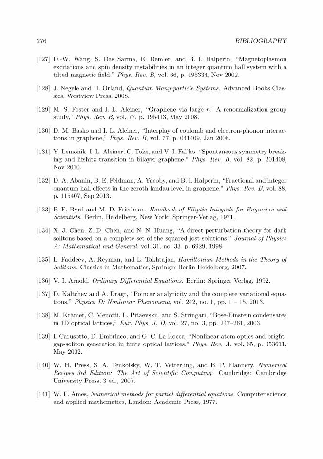
276 BIBLIOGRAPHY
[127] D.-W. Wang, S. Das Sarma, E. Demler, and B. I. Halperin, “Magnetoplasmonexcitations and spin density instabilities in an integer quantum hall system with atilted magnetic field,” Phys. Rev. B, vol. 66, p. 195334, Nov 2002.
[128] J. Negele and H. Orland, Quantum Many-particle Systems. Advanced Books Clas-sics, Westview Press, 2008.
[129] M. S. Foster and I. L. Aleiner, “Graphene via large n: A renormalization groupstudy,” Phys. Rev. B, vol. 77, p. 195413, May 2008.
[130] D. M. Basko and I. L. Aleiner, “Interplay of coulomb and electron-phonon interac-tions in graphene,” Phys. Rev. B, vol. 77, p. 041409, Jan 2008.
[131] Y. Lemonik, I. L. Aleiner, C. Toke, and V. I. Fal’ko, “Spontaneous symmetry break-ing and lifshitz transition in bilayer graphene,” Phys. Rev. B, vol. 82, p. 201408,Nov 2010.
[132] D. A. Abanin, B. E. Feldman, A. Yacoby, and B. I. Halperin, “Fractional and integerquantum hall effects in the zeroth landau level in graphene,” Phys. Rev. B, vol. 88,p. 115407, Sep 2013.
[133] P. F. Byrd and M. D. Friedman, Handbook of Elliptic Integrals for Engineers andScientists. Berlin, Heidelberg, New York: Springer-Verlag, 1971.
[134] X.-J. Chen, Z.-D. Chen, and N.-N. Huang, “A direct perturbation theory for darksolitons based on a complete set of the squared jost solutions,” Journal of PhysicsA: Mathematical and General, vol. 31, no. 33, p. 6929, 1998.
[135] L. Faddeev, A. Reyman, and L. Takhtajan, Hamiltonian Methods in the Theory ofSolitons. Classics in Mathematics, Springer Berlin Heidelberg, 2007.
[136] V. I. Arnold, Ordinary Differential Equations. Berlin: Springer Verlag, 1992.
[137] D. Kaltchev and A. Dragt, “Poincar analyticity and the complete variational equa-tions,” Physica D: Nonlinear Phenomena, vol. 242, no. 1, pp. 1 – 15, 2013.
[138] M. Kramer, C. Menotti, L. Pitaevskii, and S. Stringari, “Bose-Einstein condensatesin 1D optical lattices,” Eur. Phys. J. D, vol. 27, no. 3, pp. 247–261, 2003.
[139] I. Carusotto, D. Embriaco, and G. C. La Rocca, “Nonlinear atom optics and bright-gap-soliton generation in finite optical lattices,” Phys. Rev. A, vol. 65, p. 053611,May 2002.
[140] W. H. Press, S. A. Teukolsky, W. T. Vetterling, and B. P. Flannery, NumericalRecipes 3rd Edition: The Art of Scientific Computing. Cambridge: CambridgeUniversity Press, 3 ed., 2007.
[141] W. F. Ames, Numerical methods for partial differential equations. Computer scienceand applied mathematics, London: Academic Press, 1977.
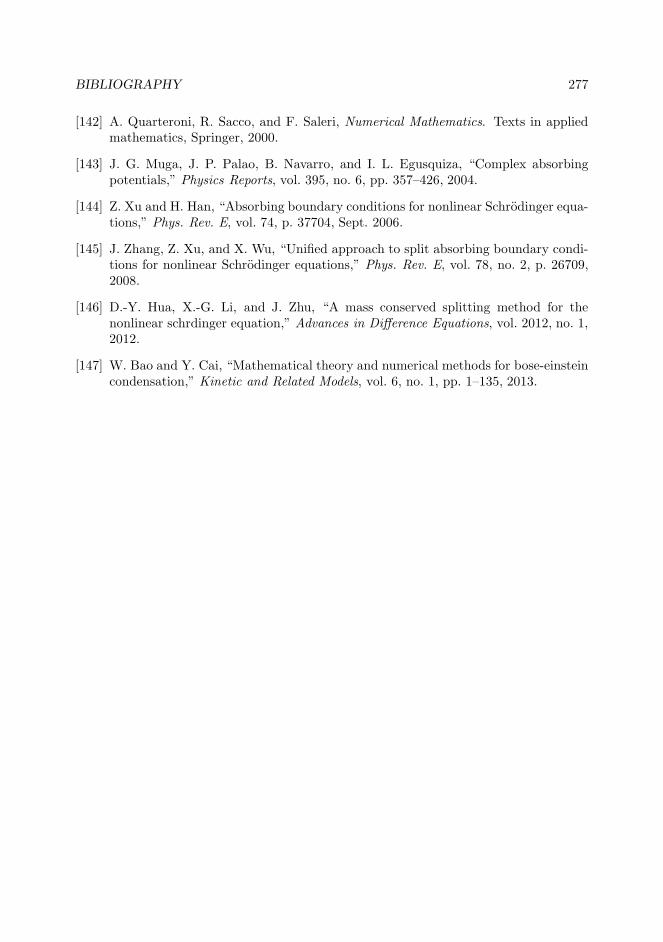
BIBLIOGRAPHY 277
[142] A. Quarteroni, R. Sacco, and F. Saleri, Numerical Mathematics. Texts in appliedmathematics, Springer, 2000.
[143] J. G. Muga, J. P. Palao, B. Navarro, and I. L. Egusquiza, “Complex absorbingpotentials,” Physics Reports, vol. 395, no. 6, pp. 357–426, 2004.
[144] Z. Xu and H. Han, “Absorbing boundary conditions for nonlinear Schrodinger equa-tions,” Phys. Rev. E, vol. 74, p. 37704, Sept. 2006.
[145] J. Zhang, Z. Xu, and X. Wu, “Unified approach to split absorbing boundary condi-tions for nonlinear Schrodinger equations,” Phys. Rev. E, vol. 78, no. 2, p. 26709,2008.
[146] D.-Y. Hua, X.-G. Li, and J. Zhu, “A mass conserved splitting method for thenonlinear schrdinger equation,” Advances in Difference Equations, vol. 2012, no. 1,2012.
[147] W. Bao and Y. Cai, “Mathematical theory and numerical methods for bose-einsteincondensation,” Kinetic and Related Models, vol. 6, no. 1, pp. 1–135, 2013.
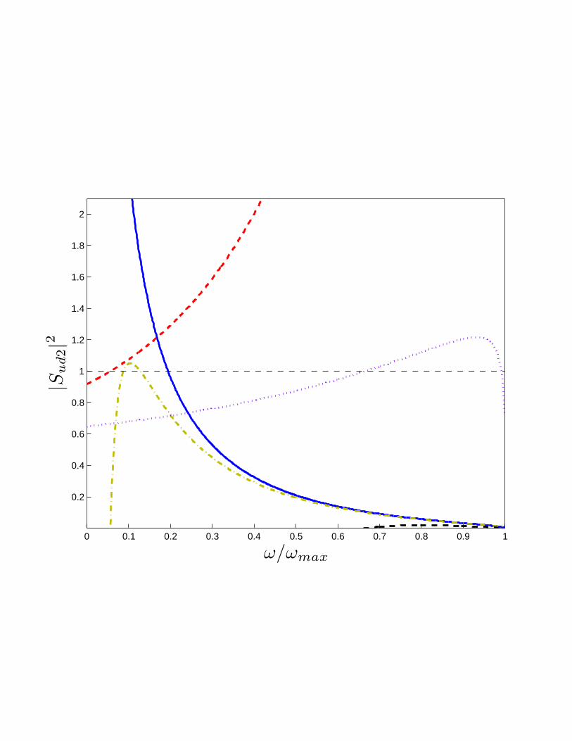
0 0.1 0.2 0.3 0.4 0.5 0.6 0.7 0.8 0.9 1
0.2
0.4
0.6
0.8
1
1.2
1.4
1.6
1.8
2
ω/ωmax
|Su
d2|2

0.1 0.3 0.5 0.7 0.9
0.5
1
1.5
2
|Sud
2|2
max

0.1 0.2 0.3 0.4 0.5 0.6 0.7 0.8 0.9
0.05
0.1
0.15
0.2
0.25
ω (mc2
0)
|Su
d2|2
0.4 0.6 0.8
0.2
0.4
0.6
0.8
ω (mc2
0)
104×
|Su
d2|2
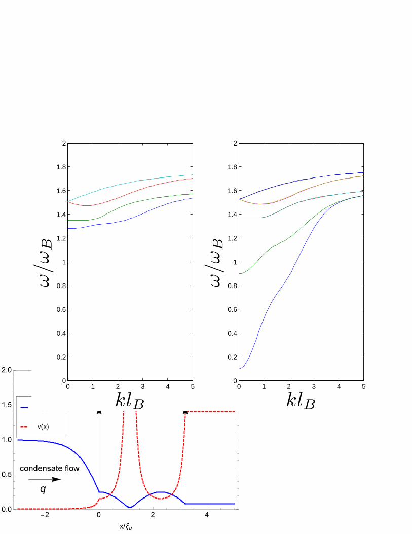
0 1 2 3 4 50
0.2
0.4
0.6
0.8
1
1.2
1.4
1.6
1.8
2
klB
ω/ω
B
0 1 2 3 4 50
0.2
0.4
0.6
0.8
1
1.2
1.4
1.6
1.8
2
klB
ω/ω
B

0.1 0.2 0.3 0.4 0.5 0.6 0.7 0.8 0.9 10
0.1
0.2
0.3
0.4
0.5
0.6
0.7
0.8
0.9
1
c2
v
X=10
CESGS
n = 0n = 1
n = 3
n = 2

0 0.5 1 1.5 2 2.5 3 3.5 4 4.5 5
−0.2
0
0.2
0.4
0.6
0.8
1
klB
ω/ω
B

1150 1200 1250 1300 1350 1400 1450 1500 1550 1600
0
0.2
0.4
0.6
0.8
1
x/ξ0
vel
oci
ty(c
0)
1150 1200 1250 1300 1350 1400 1450 1500 1550 1600
0
0.2
0.4
0.6
0.8
1
ener
gy(m
c2 0)
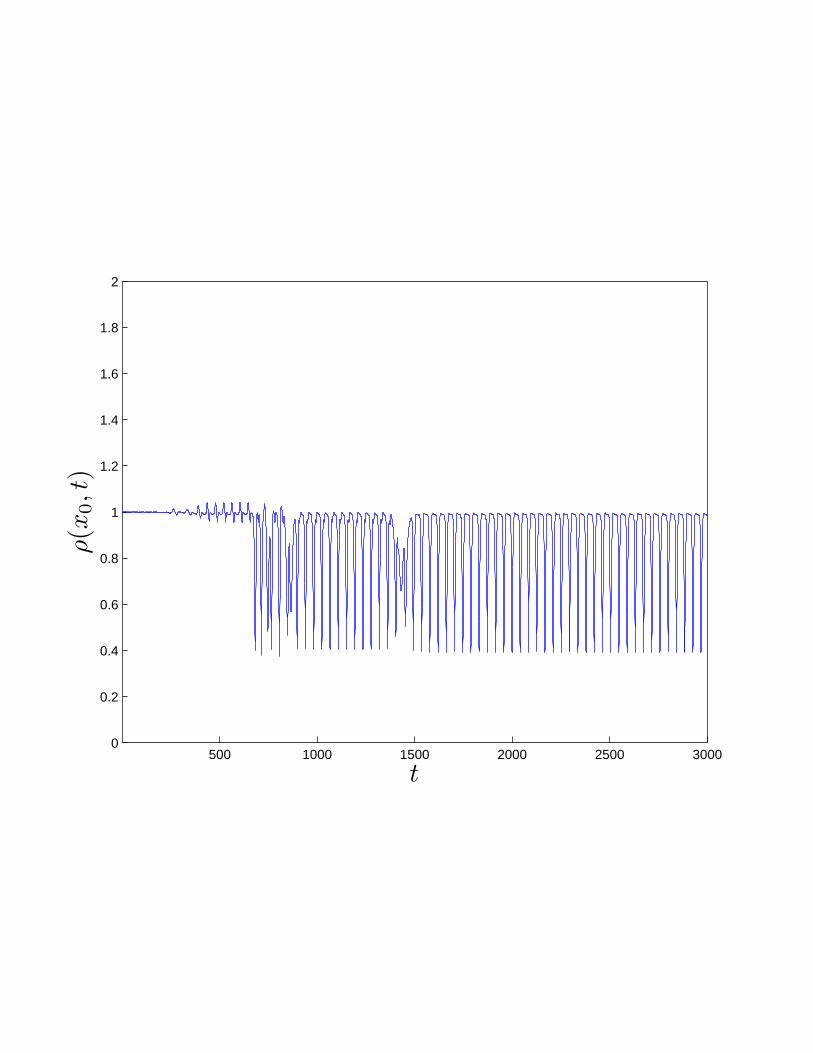
500 1000 1500 2000 2500 30000
0.2
0.4
0.6
0.8
1
1.2
1.4
1.6
1.8
2
t
ρ(x
0,t
)
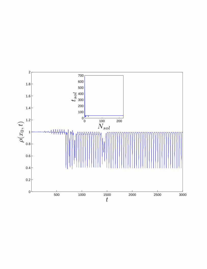
500 1000 1500 2000 2500 30000
0.2
0.4
0.6
0.8
1
1.2
1.4
1.6
1.8
2
t
ρ(x
0,t
) 0 100 2000
100
200
300
400
500
600
700
Nsol
t sol
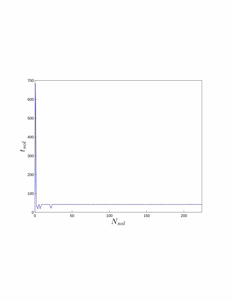
0 50 100 150 2000
100
200
300
400
500
600
700
Nsol
t sol


![arXiv:2002.10391v1 [math.DG] 24 Feb 2020SPECIAL LAGRANGIANS, LAGRANGIAN MEAN CURVATURE FLOW AND THE GIBBONS{HAWKING ANSATZ JASON D. LOTAY AND GONCALO OLIVEIRA Abstract. The Gibbons{Hawking](https://img.dokumen.tips/doc/110x75/5fb36de7a1686a5f1e5398b1/arxiv200210391v1-mathdg-24-feb-2020-special-lagrangians-lagrangian-mean-curvature.jpg)

![Black Hole EntropyandSoft Hair arXiv:1810.01847v4 [hep-th ... · arXiv:1810.01847v4 [hep-th] 13 Dec 2018 Black Hole EntropyandSoft Hair Sasha Haco∗†, Stephen W. Hawking∗, Malcolm](https://img.dokumen.tips/doc/110x75/5c7b8c8609d3f2352a8bc38d/black-hole-entropyandsoft-hair-arxiv181001847v4-hep-th-arxiv181001847v4.jpg)