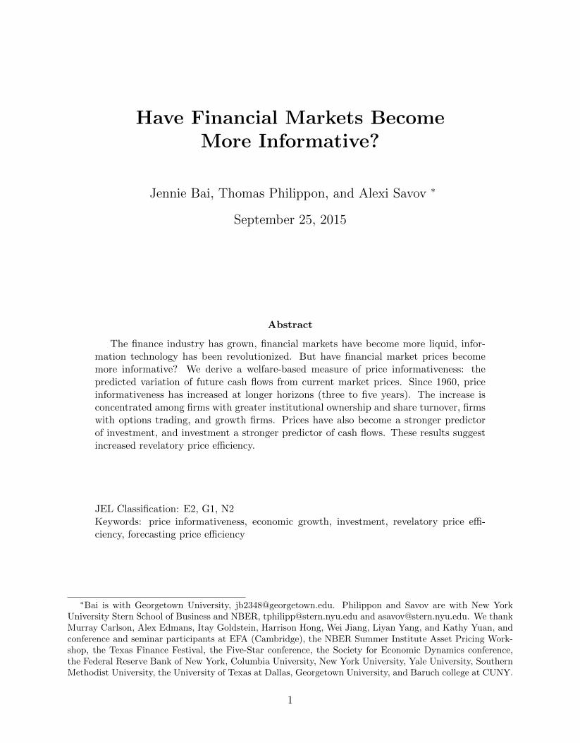
Have Financial Markets BecomeMore Informative?

Jennie Bai, Thomas Philippon, and Alexi Savov ∗

September 25, 2015

Abstract

The finance industry has grown, financial markets have become more liquid, infor-mation technology has been revolutionized. But have financial market prices becomemore informative? We derive a welfare-based measure of price informativeness: thepredicted variation of future cash flows from current market prices. Since 1960, priceinformativeness has increased at longer horizons (three to five years). The increase isconcentrated among firms with greater institutional ownership and share turnover, firmswith options trading, and growth firms. Prices have also become a stronger predictorof investment, and investment a stronger predictor of cash flows. These results suggestincreased revelatory price efficiency.

JEL Classification: E2, G1, N2Keywords: price informativeness, economic growth, investment, revelatory price effi-ciency, forecasting price efficiency

∗Bai is with Georgetown University, jb2348@georgetown.edu. Philippon and Savov are with New YorkUniversity Stern School of Business and NBER, tphilipp@stern.nyu.edu and asavov@stern.nyu.edu. We thankMurray Carlson, Alex Edmans, Itay Goldstein, Harrison Hong, Wei Jiang, Liyan Yang, and Kathy Yuan, andconference and seminar participants at EFA (Cambridge), the NBER Summer Institute Asset Pricing Work-shop, the Texas Finance Festival, the Five-Star conference, the Society for Economic Dynamics conference,the Federal Reserve Bank of New York, Columbia University, New York University, Yale University, SouthernMethodist University, the University of Texas at Dallas, Georgetown University, and Baruch college at CUNY.

1

Fama (1970) writes, “The primary role of the capital market is allocation of ownership of

the economy’s capital stock. In general terms, the ideal is a market in which prices provide

accurate signals for resource allocation: that is, a market in which firms can make production-

investment decisions . . . under the assumption that security prices at any time ‘fully reflect’

all available information.” Since these words were written, financial markets have been trans-

formed: information processing costs have plummeted, and information availability has vastly

expanded. Trading costs have fallen, and liquidity has increased by orders of magnitude. In-

stitutional investing has become dominant, and spending on price discovery has increased.1

The financial sector’s share of output has doubled. To assess whether these changes have

brought us closer to Fama’s ideal, in this paper we ask: Have financial market prices become

more informative?

To answer this question, we derive a welfare-based measure of price informativeness and

then document its evolution over time. Using U.S. stock market data from 1960 to 2014, we

find that among comparable firms price informativeness has increased substantially at medium

and long horizons (three to five years) while remaining stable at short horizons (one year).

Results from a variety of tests support the interpretation that the rise in price informativeness

is due to greater information production in financial markets. Under this interpretation, rising

price informativeness has contributed to an increase in the efficiency of capital allocation in

the economy.

We use a simple framework to derive the right, welfare-relevant measure of informativeness

and generate testable predictions. Standard q-theory (Tobin 1969) implies that investment is

proportional to the conditional expectation of future cash flows, making firm value convex in

this expectation. Intuitively, investment is an option on information, and firm value embeds

the value of this option. It follows that aggregate efficiency is increasing in information (Hayek

1945), which can be quantified by the predicted variance of future cash flows (i.e. the variance

of their conditional expectation). We are particularly interested in the information content

of prices, which is given by the predicted variance of cash flows using market prices as the

conditioning variable. Our price informativeness measure is its square root.

1Using numbers from French (2008), spending on price discovery has risen from 0.3% to 1% of GDP since1980.

2

We construct time series of price informativeness from yearly cross-sectional regressions

of future earnings on current stock market valuation ratios (we also include current earnings

and sector controls). We focus on the one-, three-, and five-year forecasting horizons and on

S&P 500 firms whose stable characteristics allow for a fairly clean comparison over time. We

show that price informativeness is increasing with horizon, consistent with prices capturing

differences in growth rates between firms. Moreover, current earnings are already a good

predictor of next year’s earnings, making prices more useful at longer horizon. From a capital

allocation perspective, the longer horizons are particularly important since the time-to-build

literature suggests that investment plans take over a year to implement, with the cash flows

materializing farther down the road.

Our key result is that price informativeness has increased substantially at the three- and

five-year horizons. The upward trend is steady throughout the fifty-year sample and its

cumulative effect is economically significant: price informativeness is about 60% higher in 2010

than 1960 at the three-year horizon and 80% higher at the five-year horizon. The increase is

highly statistically significant. Price informativeness at the one-year horizon, which is smaller

to begin with, shows a modest cumulative increase.

The increase in price informativeness is not explained by changes in return predictability.

Since valuations are driven by either cash flows or expected returns (Campbell and Shiller

1988), a decrease in cross-sectional return predictability (e.g. a drop in the value premium)

could make price informativeness rise even if information production does not. We find that

this is not the case by putting returns on the left side of our forecasting regressions, which

shows that the predictable component of returns remains stable.2

Theory suggests that the information contained in market prices for future earnings should

also be reflected in investment decisions. We therefore look at the predicted variance of in-

vestment based on market prices. We find that market prices have become stronger predictors

2For completeness, we also calculate price informativeness for firms beyond the S&P 500. We stress,however, that the composition of this sample has changed dramatically over the years (see Fama and French2004), making this comparison potentially misleading. This is readily apparent from trends in observablecharacteristics such as idiosyncratic volatility and earnings dispersion (measures of uncertainty), which haverisen drastically. By contrast, these characteristics are remarkably stable for S&P 500 firms. Likely as aresult of the compositional shift, price informativeness for firms beyond the S&P 500 appears to decline.Interestingly, the decline is concentrated at the short horizon so again there is relative improvement at thelong end. Above all, we view these results as motivating our focus on S&P 500 firms.

3

of investment as measured by R&D spending (though not CAPX). Thus, when it comes to

real decisions like R&D, for which market information is arguably particularly useful, the

information content of prices has also increased.

It is important to note that more informative prices do not necessarily imply that financial

markets have generated an improvement in welfare. Market prices contain information pro-

duced independently by investors, as well as information disclosed by the firm. It is mainly

the independent, market-produced component of price informativeness that contributes to

the efficiency of capital allocation. Bond, Edmans, and Goldstein (2012) call this component

“revelatory price efficiency” (RPE), in contrast to“forecasting price efficiency” (FPE) which

also includes information already known to decision makers inside the firm.

Although separating FPE and RPE is challenging, we can use our theoretical framework

to guide our analysis. In our framework, managers have access to internal information, some

of which they disclose to the market. Investors combine this disclosure with their own inde-

pendent information to trade, and this causes prices to incorporate both types of information

(FPE). Managers then filter out as much of the independent information contained in prices

as they can (RPE) and combine it with their own internal information to set investment op-

timally (aggregate efficiency). The rich two-way feedback between firms and markets in our

framework ensures that the predictions we formulate and test are robust to a wide range of

models proposed in the literature.

Our framework shows that it is possible to distinguish an increase in market-produced

information (RPE) from a pure increase in firm disclosure by looking at aggregate efficiency,

the predicted variation of future cash flows based on the manager’s full information set. All

else equal, an increase in disclosure causes aggregate efficiency to remain the same even as

price informativeness (FPE) rises. Although the manager’s information set is not observed, it

gets reflected in her investment decisions. Specifically, we show that we can bound aggregate

efficiency from below by the predicted variation of future cash flows from investment and

from above by the cross-sectional dispersion of investment, both of which are increasing in the

amount of information the manager has. Measuring investment as either R&D alone or R&D

and CAPX together, we find evidence that the predicted variation of earnings from investment

has increased. We also find that the cross-sectional dispersion of R&D has increased. This

4

suggests that aggregate efficiency has increased. Combined with the observed rise in price

informativeness (FPE), the increase in aggregate efficiency supports the interpretation that

market-based information production (RPE), and not just disclosure, has increased.

While we are thus able to rule out a rise in disclosure as the sole explanation for the rise

in price informativeness, a more subtle explanation remains: it could be that information

production inside firms and disclosure have both increased. The former would explain the rise

in aggregate efficiency while the latter would explain the rise in price informativeness. Teasing

out this more complicated explanation is challenging and it requires additional predictions we

can test. We construct and test four such predictions that exploit cross-sectional differences

between firms. While none of our tests is perfect, we find that the overall evidence supports

the interpretation that market-based information production (RPE) has increased.

Our first cross-sectional prediction is that market-based information production should

be higher for firms with high institutional ownership. Institutional investors have come to

dominate financial markets, their stake in the average firm rising from 20% in 1980 to 60% in

2014. Given their professional expertise, we expect them to have a large impact on market-

based information production. In our test, we compare firms with institutional ownership

above and below the median, going beyond the S&P 500 to obtain greater cross-sectional

variation. Interestingly, dispersion has increased so that the gap in institutional ownership

between the two groups has widened. We find that price informativeness is both higher and

has increased more for the group with high and increasing institutional ownership. This result

is consistent with the RPE view that information production in markets has increased.

In our second cross-sectional test, we compare the price informativeness of stocks with and

without option listings and stocks with high and low levels of options trading. The CBOE

began listing options in 1973 and has been adding new listings in a staggered manner. Our

test is based on the idea that options provide traders with leverage, the ability to hedge, and

a low-cost way to sell short, all of which increase the incentive and scope for market-based

information production. We find that price informativeness has increased more for CBOE-

listed firms than for non-listed firms and that price informativeness is higher for firms with

higher levels of option turnover. These findings are also consistent with the RPE view.

In our third test, we compare firms with high and low levels of liquidity as proxied by

5

share turnover. The idea is that greater liquidity facilitates the incorporation of private

information into prices. It also increases the incentives of market participants to produce such

information. Consistent with this idea, we find that stocks with higher turnover have higher

price informativeness. Since liquidity in general and turnover in particular have increased

strongly over the past five decades, this finding helps to explain the observed rise in overall

price informativeness and supports the view that RPE has increased.

For our final cross-sectional test, we enrich our model with cross-sectional differences be-

tween firms. Specifically, we incorporate the natural feature that a firm’s cash flows from

growth options may not be perfectly correlated with its cash flows from assets in place. The

idea is that firm insiders hold an advantage in producing information about assets in place,

after all they are the ones who put them there. Valuing growth options, on the other hand,

requires making comparisons to other firms and analyzing market trends, and here the mar-

ket may have the advantage or at least less of a disadvantage. Based on this reasoning, if

market-based information has increased we would expect price informativeness to increase

more for firms with a lot of growth options (growth firms), whereas if internal information

and disclosure have increased we would expect greater improvement among firms with fewer

growth options (i.e. value firms). Consistent with the market-based RPE view, we find that

price informativeness has risen much more for growth firms than for value firms. This result is

interesting from a broader perspective as it indicates that the increase in price informativeness

is concentrated among hard-to-value firms where it is most needed.

The rest of this paper proceeds as follows: Section 1 reviews the literature, Section 2

derives our informativeness measure, Section 3 describes the data, Section 4 presents results,

and Section 5 concludes.

1 Related literature

Levine (2005) categorizes the economic role of the financial sector into five channels: (1) infor-

mation production about investment opportunities and allocation of capital; (2) mobilization

and pooling of household savings; (3) monitoring of investments and performance; (4) financ-

ing of trade and consumption; and (5) provision of liquidity, facilitation of secondary market

6

trading, diversification, and risk management. Our focus is on documenting (1) empirically.

The information production role of financial markets is part of a classic literature in eco-

nomics going back at least to Schumpeter (1912) and Hayek (1945). Greenwood and Jovanovic

(1990) and King and Levine (1993b) provide endogenous growth models in which informa-

tion production in financial markets enables efficient investment. We derive a welfare-based

measure of price informativeness that is in the spirit of this literature, one that can be easily

taken to the data.

The empirical literature on finance and growth largely relies on cross-country comparisons.

Examples include King and Levine (1993a), Rajan and Zingales (1998), Morck, Yeung, and

Yu (2000), and Bekaert, Harvey, and Lundblad (2001). Our novel methodology exploits firm-

level variation, which allows us to examine the information production channel within a single

country, in our case the U.S., over time.

The U.S. time series represents a particularly important setting because over the last few

decades the U.S. financial sector has grown six times faster than GDP (Philippon 2015). At

its peak in 2006, it contributed 8.3% to U.S. GDP compared to 2.8% in 1950 (see Philippon,

2015, and Greenwood and Scharfstein, 2012, for in-depth discussions). Finance has also drawn

in a large share of human capital (Philippon and Reshef 2012). The question arises whether

these changes have led to an increase in economic efficiency. While it is difficult to discern

such a relationship in aggregate U.S. data, we provide a partial answer to this question by

using cross-sectional data to examine the informativeness of financial market prices.

The answer is by no means clear a priori. The dot-com bust of 2000 and the financial crisis

of 2008 have called the benefits of financial development into question (e.g. Zingales 2015).

Prices can be distorted due to behavioral biases (e.g. Hong and Stein 1999; Shiller 2000),

or incentives (e.g. Rajan 2005). Gennaioli, Shleifer, and Vishny (2012) argue that financial

innovation can increase fragility. Bolton, Santos, and Scheinkman (2011) provide a model in

which rents in the financial sector attract an excessive share of the economy’s human capital.

Philippon and Reshef (2012) document a potentially distorting wage premium in the financial

sector and Philippon (2015) finds that the unit cost of financial intermediation has remained

relatively high in recent decades. Quantifying information production as we do in this paper

contributes to this important effort of measuring value added in the financial sector.

7

A large theoretical literature with seminal papers by Grossman and Stiglitz (1980), Glosten

and Milgrom (1985), Kyle (1985), and Holmstrom and Tirole (1993) studies the incentives of

traders to produce information. As financial technology develops and the cost of producing

information shrinks, the information content of prices increases. The information revolution

and the growth of financial markets suggest that the premise of this proposition is in place.

Our contribution is to assess its implication.

Bond, Edmans, and Goldstein (2012) survey the literature on information production in

financial markets, emphasizing the challenge of separating the genuinely new information pro-

duced in markets, which they call revelatory price efficiency (RPE), from what is already

known and merely reflected in prices which they call forecasting price efficiency (FPE). This

distinction can be traced back to Hirshleifer (1971) and Tobin (1984). We follow this con-

ceptual framework and seek to disentangle RPE and FPE by measuring the efficiency of

investment and by comparing groups of firms where RPE or FPE is expected to prevail.

Recent theoretical work on asset prices and real efficiency includes Dow and Gorton (1997),

Subrahmanyam and Titman (1999), Goldstein and Guembel (2008), Ozdenoren and Yuan

(2008), Bond, Goldstein, and Prescott (2010), Goldstein, Ozdenoren, and Yuan (2013), Kurlat

and Veldkamp (2015), and Edmans, Goldstein, and Jiang (2015). While these papers share

the basic feedback from market prices to investment that is the subject of our paper, each

focuses on a particular form of more advanced feedback such as that from investment to

market prices. In Section 2, we use our theoretical framework to discuss these papers in some

detail, and we derive the predictions we test based on their common features.

On the empirical side, Chen, Goldstein, and Jiang (2007) and Bakke and Whited (2010)

find that the relationship between stock prices and investment is stronger for firms with more

informative stock prices, whereas Baker, Stein, and Wurgler (2003) find that it is stronger for

firms that issue equity more often. Turley (2012) exploits a regulatory change to show that

lower transaction costs increase short-term (one to three month) stock price informativeness.

Our contribution here is to examine the evolution of price informativeness over a long period

of time characterized by unprecedented growth in the financial sector.

The most common measure of informativeness is price non-synchronicity (Roll 1988), which

is based on the correlation between a firm’s return and a market or industry benchmark (a

8

high correlation is interpreted as lower informativeness). Papers that adopt this measure

include Morck, Yeung, and Yu (2000), Durnev, Morck, Yeung, and Zarowin (2003), and

Chen, Goldstein, and Jiang (2007). Durnev, Morck, Yeung, and Zarowin (2003) show that

price non-synchronicity is positively related to the correlation between returns and future

earnings at the industry level, which helps to validate it as a measure of informativeness. A

second popular measure comes from the microstructure literature: the probability of informed

trading or PIN (Easley, Kiefer, O’Hara, and Paperman 1996), which is based on order flow.

Our contribution here is to derive a welfare-based measure which quantifies the information

contained in prices for real outcomes and is easily computed from widely available data.

Our paper is also related to the accounting literature on disclosure (see surveys by Healy

and Palepu (2001) and Beyer, Cohen, Lys, and Walther (2010)). Our sample includes some

significant changes in disclosure requirements, most prominently Regulation Fair Disclosure

in 2000 and Sarbanes-Oxley in 2002. Considerable debate remains regarding the effects of

these reforms; even their sign is unsettled.3 We find no evidence of structural breaks in

informativeness around their passage. In addition, our result that aggregate efficiency has

increased makes it unlikely that changes in disclosure alone can explain the observed rise in

price informativeness.

A second related strand of the accounting literature studies value relevance, the impact of

accounting metrics on market values (see e.g. Holthausen and Watts (2001) and Dechow, Zha,

and Sloan (2014)). This literature establishes both that earnings information drives returns

and that returns do not always fully incorporate earnings information. This is one reason

why we include current earnings as a control in our forecasting regressions. There is also

evidence that the value relevance of earnings has actually declined over our sample (Collins,

Maydew, and Weiss 1997), which would bias our results downward. We show that our main

result holds under a variety of accounting metrics, including different measures of earnings

and operating cash flows. The broader difference between this literature and our paper is that

we measure the extent to which market values predict—as opposed to react to—accounting

3Heflin, Subramanyam, and Zhang (2003) find no evidence of increased earnings surprises in returns afterReg. FD, suggesting that the information available to market participants was not reduced. On the otherhand, Wang (2007) reports that firms cut back on issuing earnings guidance reports after Reg. FD. YetBushee, Matsumoto, and Miller (2004) provide evidence that disclosure remained constant or even increasedafter Reg. FD.

9

metrics, specifically earnings and investment.

In sum, our paper lies at the intersection of the finance-and-growth literature and the

literature on information production in financial markets. Its underlying premise is that

measuring price informativeness over time helps to assess the economic value of a growing

financial sector.

2 Theoretical framework and discussion

We present a theoretical framework with two goals in mind. The first is to derive a welfare-

based measure of price informativeness that we can use in our empirical analysis. The second

is to formulate testable predictions that we can use to interpret our results. We also discuss

these predictions in the context of the existing literature.

Our framework has two essential components: a q-theory/aggregate efficiency block and

an information environment block.

Q-theory and aggregate efficiency: Consider a firm with ex-post fundamental value as in stan-

dard q-theory following Hayashi (1982):

v (z, k) = (1 + z)(k + k

)− k − γ

2kk2, (1)

where k represents assets in place, k is investment in new capital, z is a productivity shock,

and γ is an adjustment cost parameter.

Investment is chosen to maximize firm value under the manager’s (more generally, the

decision maker’s) information set Im: k? = argmaxk E [v (z, k)| Im]. We have normalized the

discount rate to zero for simplicity (we address discount rates in Section 4.3). This leads to

the well-known q-theory investment equation

γk?

k= E [z | Im] . (2)

The investment rate k?/k is proportional to the conditional expectation of net productivity z

10

given the manager’s information set. The maximized ex-post firm value is then

v (z, k?)

k= 1 + z +

z

γE [z| Im]− 1

2γE [z| Im]2 . (3)

We can also write the expected firm value conditional on investment and the information

available to the manager as

E[v (z, k?)

k

∣∣∣∣ Im] = 1 + E [z| Im] +1

2γ(E [z | Im])2 . (4)

We are interested in the efficiency of capital allocation across firms, so we consider a large

number of ex-ante identical firms (same k) that draw different signals about z. We normalize

z to have mean of zero across these firms. Aggregate efficiency is then defined by the ex-ante

(or cross-sectional average) firm value

E [v (z, k?)] = k +k

2γVar (E [z| Im]) . (5)

Aggregate efficiency is a function of the variance of the forecastable component of net pro-

ductivity z. This is the first key theoretical point that we use in our empirical analysis. The

next step is to think about how Im is determined in equilibrium.

Information environment: In practice, managers have access to information produced inside

the firm, as well as to outside information contained in market prices. We summarize the

internal information with the signal

η = z + εη, (6)

where εη ∼ N(0, σ2

η

). The price-based information is contained in the price p of a security

linked to the firm’s payoff. This information contained in p is itself derived from the private

information of informed traders in the market for this security. We summarize the information

of these informed traders with the signal

s = z + εs, (7)

11

where εs ∼ N (0, σ2s). We assume that εη and εs are independent, so we can think of η and s

as the two fundamental sources of information that society can use to improve efficiency.

In practice market participants and managers also share common sources of information

other than prices, most prominently through disclosure. To take this into account, we assume

that traders observe an additional signal coming from the manager:

η′ = η + εη′ , (8)

where εη′ ∼ N(0, σ2

η′

)is orthogonal to εη and εs. The disclosure signal η′ captures the flow

of information from the firm to the market, which runs in the opposite direction of the flow

of information from the market to the firm in the form of the price p. To summarize, the

information set of the manager is Im = {η, η′, p} and the information set of informed traders

is Iτ = {η′, s}.

Feedback and equilibrium: A full-fledged model needs to specify the objectives of the traders

(e.g. CARA or mean variance preferences, constraints, etc.) as well as a trading protocol (e.g.

competitive or strategic, with or without market makers, etc.). We present one such model in

Appendix A, but for the purpose of this discussion it is more important to focus on the key

features shared by nearly all models.

We must first specify exactly which security is traded in financial markets. Recall that v

is the total value of the firm. In practice, it can be the case that equity is publicly traded but

debt it not, or perhaps that the traded security is an option or a credit derivative. So let us

define F (z, k) as the payoff of the claim that is traded in financial markets. An important

particular case is of course F (z, k) = v (z, k) with v (·) as in equation (3). Since the informed

traders’ information set consists of η′ and s, the equilibrium price typically takes the form

p = αE [F (z, k?)| η′, s] + βu, (9)

where u is noise trading demand, and α and β are endogenous coefficients that are part of the

rational expectations equilibrium. Exactly how to solve for these coefficients, and whether

we actually obtain a linear price function depends on the details of the model. The more

12

tractable models, including our appendix model, result in pricing functions of the form in (9).

Equilibrium and basic feedback: To summarize, most models in the literature boil down to

two equations which we restate for convenience:

k? =k

γE [z| η, η′, p] (10)

p = αE [F (z, k?)| η′, s] + βu. (11)

The basic feedback is that managers learn from prices and so k? depends on p. It implies that

the informativeness of prices matters for firm value, aggregate efficiency, and welfare. This

feature, which is the most important one for our analysis, is common to all models we discuss

below, even though they differ in the complexity of the other interactions between value and

prices.

Advanced feedback: The more advanced feedback channels depend on the nature of the traded

claim and on the trading protocol. For instance, Subrahmanyam and Titman (1999) make the

simplifying assumption F (z, k?) = z to ensure linearity of the conditional expectations. In

that case the pricing equation (11) does not depend on the mapping k? in (10) and the model

remains linear and tractable. Our model in Appendix A adopts this approach and discusses

its implications. It can be interpreted as a linear approximation to a more complex model

when k?/k is not too large as is the case in the data.

Other papers (e.g. Goldstein, Ozdenoren, and Yuan 2013) use the more complex but also

richer case F = v. In that case, p can be interpreted as the market value of the firm. Firm

value is a nonlinear function of z and k?, so finding p involves solving a complex fixed-point

problem. The traders need to form beliefs about the function k?, i.e. about how the manager

uses prices to decide on investment. Traders then use these beliefs to forecast total firm value

and this determines the equilibrium price. Dow and Gorton (1997) show that this can lead to

multiple equilibria.4 In one equilibrium managers invest based on prices and this gives traders

4In their model managers are clueless, σ2η =∞, and returns on assets in place are independent of z, which

is indeed precisely the opposite assumption from Subrahmanyam and Titman (1999). Ozdenoren and Yuan(2008) work with another tractable alternative, F = k? + z, similarly assuming σ2

η =∞. In Bond, Goldstein,and Prescott (2010), σ2

η <∞ but σ2s = 0 so traders have perfect information.

13

an incentive to gather information. In the other equilibrium prices are not informative and

managers do not invest. Goldstein and Guembel (2008) show that the basic feedback can

give incentives to a large uninformed speculator to manipulate the stock price by short-selling

the stock, inducing inefficient disinvestment, reducing firm value, and thereby making the

short-selling strategy profitable. Conversely, Edmans, Goldstein, and Jiang (2015) emphasize

the strategic behavior of a large informed trader who knows that whatever information she

reveals will be used to increase firm value. This leads to asymmetric revelation of good and

bad news. These effects rely on the basic feedback and on the strategic behavior of large

traders who understand that they influence prices.

Empirical predictions: The framework outlined above offers a precise overview of the existing

literature. Our next task is to formulate specific predictions that we can test empirically.

We begin by quantifying price informativeness, i.e. the forecasting power of prices for

future cash flows, which Bond, Edmans, and Goldstein (2012) call forecasting price efficiency

(FPE). We scale by k to allow for meaningful comparisons across firms, and we define a firm’s

market to book ratio q = p/k. FPE is given by the variance of the predictable component

of firm value v/k given q. From (3), v/k has some nonlinear terms in z, but to a first-order

approximation v/k ≈ 1 + z, so we will focus on

VFPE ≡ Var (E [z| q]) . (12)

FPE measures the total amount of information about future payoffs contained in market

prices. At the same time, it is only a forecasting concept. As explained above, aggregate

efficiency depends on the information of the manager:

VM ≡ Var (E [z| η, η′, q]) . (13)

We are interested in the part of VM that comes from market prices. This is what Bond,

Edmans, and Goldstein (2012) call revelatory price efficiency (RPE). It is given by

VRPE ≡ Var (E [z| η, η′, q])− Var (E [z| η, η′]) . (14)

14

RPE measures the extent to which prices improve real allocations. When prices are uninfor-

mative or when managers already know the information they contain, RPE is low. On the

other hand, when prices provide managers with information that is useful for improving the

efficiency of investment, RPE is high. This is the core idea of Hayek (1945).

Each of the theoretical models discussed above gives an explicit mapping from the funda-

mental information structure (σ2s , σ

2η, σ

2η′) into the objects of interest, VFPE and VRPE. We

cannot do justice to all the subtle predictions based on advanced feedback, but we can focus

on the predictions that are robust across models. In particular, we test the following:

Prediction 1. All else equal,

(i) a decrease in σ2s (traders produce more information) increases VFPE, VRPE and VM .

(ii) a decrease in σ2η (firms produce more information) increases VFPE and VM but not VRPE.

(iii) a decrease in σ2η′ (firms disclose more information) increases VFPE but neither VM nor

VRPE.

When traders produce more information (their signal s becomes less noisy), prices become

more informative and so FPE goes up. RPE also goes up because the additional information

in prices is new to managers. As managers use this information, aggregate efficiency increases.

Aggregate efficiency also increases when managers produce more information (η becomes less

noisy), and this again causes FPE to go up through disclosure. However, in this case prices are

merely reflecting information already available managers and so RPE does not rise. Finally,

an improvement in disclosure (η′ becomes less noisy) leaves aggregate efficiency and RPE

unchanged because it does not affect the amount of information available to managers. It,

does, however, raise FPE because the additional disclosure gets reflected in prices.

Prediction 1 allows us to interpret an observed trend in FPE as coming from internal

information, from market participants, or from disclosure by looking for parallel trends in

aggregate efficiency. For instance, an increase in VFPE and VM rules out a pure disclosure

explanation (part (iii)). Separating parts (i) and (ii) then requires additional testable predic-

tions. We construct such predictions by enriching the model with cross-sectional differences

across firms after we have established the basic trends in FPE.

15

Our empirical analysis centers on Prediction 1. As we noted, this prediction is common

throughout the literature. To motivate it further, we derive Prediction 1 formally in the model

we present in Appendix A.

3 Data and summary statistics

We now describe the main aspects of our data and how we construct our sample.

Data sources: Our main sample is annual from 1960 to 2014. We obtain stock prices from

CRSP. All accounting variables are from Compustat. Institutional ownership is from 13-F

filings provided by Thomson Reuters. The test on option listings uses listing dates from

the CBOE (available after 1973 when single-name option trading began) and the test on

option turnover uses option volume data from OptionMetrics (available after 1996). The

GDP deflator used to adjust for inflation is from the Bureau of Economic Analysis.

We take stock prices as of the end of March and accounting variables as of the end of

the previous fiscal year, typically December. This timing convention ensures that market

participants have access to the accounting variables that we use as controls.

Sample selection: For most of the paper we limit attention to S&P 500 non-financial firms.

These firms represent the bulk of the value of the U.S. corporate sector. As we show, their

characteristics have remained remarkably stable, which makes them comparable over time.

This is in contrast to the broader universe of all firms, whose characteristics have changed

drastically. We report results for these firms in the appendix and summarize them in the text.

Measures: Our main equity valuation measure is the log-ratio of market capitalization M

to total assets A, logM/A.5Our main cash flow variable is earnings measured as EBIT. In

Appendix B we show that our main results are robust to using alternative measures such as

EBITDA, net income, and cash flows from operations (CFO). We focus on EBIT because it

is most widely available in Compustat and because it is the focus of analyst research. For

5The correct functional form is whichever one managers use to extract information from prices. Withidentical firms and normal shocks one could use q, the ratio of the market price to existing assets (see Section2). In practice, we find that taking logs works slightly better because it mitigates skewness in the data.

16

investment we use both research and development (R&D) and capital expenditure (CAPX).

We scale both current and future cash flows and investment by current total assets. For

instance, in a forecasting regression for earnings with horizon h years, the left-side variable

is Et+h/At. This specification is implied by our framework (see Section 2; we are predicting

v/k ≈ 1 + z). In particular, it incorporates growth between t and t+ h. Unlike prices, we do

not take logs because it is the level of cash flows that matters for aggregate efficiency.

Correcting for delisting: We must account for firm delisting to ensure that our forecasting

regressions are free of survivorship bias.6 We do so as follows: When a firm is delisted, we

invest the delisting proceeds (calculated using the delisting price and dividend) in a portfolio

of firms in the same two-digit SIC industry. We use the earnings accruing to this portfolio to

fill in the earnings of the delisted firm. We do the same for investment.

Adjusting for inflation: We adjust for inflation with the GDP deflator. This is necessary be-

cause it is real price informativeness that matters for welfare. Since inflation is multiplicative,

differences in future nominal cash flows between firms are larger than differences in real cash

flows. This biases the forecasting coefficient up during high-inflation periods like the 1970s.7

Summary statistics: Table I presents summary statistics for our main sample of S&P 500 firms.

The first set of columns covers the full period from 1960 to 2014, whereas the second and third

sets cover its first and second half. They show that firms have become larger and their profits

have grown with the economy. Yet profitability (earnings over assets) is stable both in terms

of levels and cross-sectional dispersion. This is true of current as well as future profitability

(measured against current assets), our key left-side variables. Market valuations, our key

right-side variable, have risen with the overall market but their cross-sectional dispersion is

6Survivorship bias would arise if the relationship between market valuations and future earnings is differentamong firms that are delisted (their future earnings and investment appear as missing in our sample) thanamong firms that are not delisted. Since our focus is on trends, it is changes in delisting rates that are ofconcern. In our sample of S&P 500 firms, the delisting rate is slightly higher (3.2% per year) in the secondhalf of the sample than in the first half (2.3%). This is because most delistings occur when a firm is acquired,so delisting tracks the merger waves of the 1980s and 1990s.

7In the first circulated draft of the paper (dated December 2013) we incorrectly inferred that price informa-tiveness had remained stable. This was due to the combined effect of three differences in methodology. First,we did not adjust for inflation. This led price informativeness to be overstated in the high-inflation years ofthe 1970s and early 1980s. Second, we did not correct for delistings, which have increased somewhat in thelatter part of our sample. And third, we did not consider the long five-year horizon.

17

only slightly higher. Investment has shifted a bit from CAPX to R&D and R&D has become

more right-skewed, but overall investment rates are stable.

Figure 1 depicts the cross-sectional distribution of several characteristics over time by

plotting their median (red line) and their 10th to 90th percentile range (gray shading) in a

given year. The top two panels confirm that the distributions of the valuation ratio logM/A

and profitability E/A have remained stable, and the bottom two panels confirm that R&D

has become more right-skewed and CAPX has declined in importance.

While the underlying characteristics of these firms have changed little, their trading en-

vironment has changed drastically. As Table I shows, share turnover has increased five-fold,

institutional ownership has risen by about half, and a large majority of firms now have their

options trading on the CBOE in significant volume. These changes reflect the broader trans-

formation in financial markets that serves as the backdrop for our investigation of price infor-

mativeness. We return to them in Sections 4.5 to 4.7 below.

The stability among S&P 500 firms stands in sharp contrast to the broader sample of

all firms, whose characteristics are presented in Table A.IV and discussed in Appendix C.

Among all firms profitability has both fallen and become much more disperse. Consistent

with Campbell, Lettau, Malkiel, and Xu (2001), median idiosyncratic volatility has increased

from 9.8% to 12.3% per month (for S&P 500 firms the change is negligible from 6.4% to

6.8%). Fama and French (2004) show that these changes are related to the listing of smaller

and younger firms and to the emergence of NASDAQ. Besides being more uncertain, these

firms are arguably also harder to value since many lack a consistent earnings record. These

compositional changes imply that the sample of firms outside the S&P 500 is not comparable

over time. We present results for these firms in Appendix C for completeness.

4 Empirical results

Estimation: We construct our measure of price informativeness (FPE) by running cross-

sectional regressions of future earnings on current market prices. We include current earnings

and industry sector as controls to avoid crediting markets with obvious public information.

18

Specifically, in each year t = 1960, . . . , 2014 and at every horizon h = 1, . . . , 5, we run

Ei,t+hAi,t

= at,h + bt,h log

(Mi,t

Ai,t

)+ ct,h

(Ei,tAi,t

)+ dst,h1

si,t + εi,t,h, (15)

where i is a firm index and 1s is a sector (one-digit SIC code) indicator. Table A.I discussed

in Appendix B provides an example from 2009. These regressions give us a set of coefficients

indexed by year t and horizon h.

From Section 2, price informativeness VFPE is the predicted variance of future cash flows

from market prices (equation (12)). We compute it here with the minor change of taking a

square root, which gives meaningful units (dollars of future cash flows per dollar of current

total assets). From regression (15), price informativeness in year t at horizon h is the fore-

casting coefficient bt,h multiplied by σt (log (M/A)), the cross-sectional standard deviation of

the forecasting variable logM/A in year t:

(√VFPE

)t,h

= bt,h × σt (log (M/A)) . (16)

We are interested in how this measure has evolved over time.

Price informativeness by horizon: Figure 2 gives a first look by plotting average price infor-

mativeness by horizon and sub-period. We cap the horizon at five years to ensure that we

have enough data to produce reliable estimates. The range between one and five years also

covers the time span over which information can plausibly affect investment and investment

can produce cash flows. For instance, the time-to-build literature finds that investment plans

take about two years to implement with cash flows following in the years after that (Koeva

2000). From a capital allocation perspective, it is therefore the medium and long horizons we

look at that are especially important.

The red line in Figure 2 plots price informativeness at each horizon averaged over the

full length of the sample (from 1960 to 2014). As expected, informativeness is positive;

market prices are positive predictors of future earnings. Informativeness is also increasing

with horizon. The reason is that while current earnings are already a good predictor of

19

earnings one year fro now, prices are useful for predicting earnings farther out.8 This provides

further motivation for focusing on the longer horizons as we do.

The dashed black and dash-dotted blue lines in Figure 2 plot average price informativeness

for the first and second half of our sample. Informativeness is higher in the later half at every

horizon. The increase is itself increasing with horizon: one-year informativeness is only slightly

higher while three- and five-year informativeness show a much larger increase (we look closely

at the magnitude and significance of these increases in the next section). From here on, for

conciseness we focus on horizons of one, three, and five years (h = 1, 3, 5).

4.1 Price informativeness over time

Figure 3 plots the time series of our estimates. Each panel holds horizon fixed and looks

across time, ending in 2010 because the last years for which we have three- and five-year

estimates are 2009 and 2011, respectively (recall our sample ends in 2014). The two left

panels show the forecasting coefficients bt,h from regressions (15), the two middle panels show

price informativeness bt,h×σt (logM/A) from (16), and the two right panels show the marginal

contribution of market prices to the regression R2, which measures the fraction of the ex post

variation in future earnings that market prices capture. Above the panels are the fitted

equations for linear time trends for the three- and five-year horizon estimates. The time

trends are normalized so that the intercept measures the value of a given series in 1960 and

the slope measures its cumulative change over the full sample period. Adjacent are p-values

for the trend coefficients based on Newey-West standard errors with five lags to account for

potential autocorrelation.9

We begin by noting that the coefficients, informativeness, and marginal R2 series are always

positive, indicating that market prices are consistently positive predictors of future earnings.

8Formally, Figure A.1 in the appendix shows that while the forecasting coefficient on prices bt,h is increasingwith horizon, the forecasting coefficient on current earnings ct,h is decreasing with horizon (see Appendix Bfor details). Thus, current earnings are relatively more informative at short horizons and prices are relativelymore informative at long horizons.

9Our choice of lag is based on two considerations. The first is that our estimates come from overlappingregressions, which can induce autocorrelation (for instance our five-year estimate for 1960 uses data from 1960to 1965, that for 1961 uses data from 1961 to 1966, and so on). The longest overlap is from the five-yearhorizon, and this is why we use a lag of five (for consistency we apply the same lag at all horizons). Thesecond consideration is that the optimal lag selection procedure of Newey and West (1994) implies an optimallag of between four and five. Our results are robust to alternative choices.

20

All series are typically higher at the longer horizons, consistent with what we saw in Figure 2.

We note a drop in the three-year series at the end of the NASDAQ boom in 2000 when many

high-valuation firms turned out to have low earnings ex post, but this drop is short-lived and

does not influence the long-run trend.

Our key result is that the coefficients, marginal R2, and most importantly, the price in-

formativeness series in Figure 3 all show clear upward trends at both the three- and five-year

horizons. By contrast, the one-year series show only a mild increase. In terms of magnitudes,

three-year price informativeness is about 60% higher in 2010 than in 1960, and the increase is

highly statistically significant. Five-year informativeness is about 80% higher, also highly sig-

nificant. Although the estimates can be noisy from year to year, the upward trend is steady

throughout the five decades of our sample.10 These results show that the extent to which

market prices can be used to distinguish firms that will deliver high earnings in the future

from those that will not has increased over the past five decades.

For a more detailed look, we run regressions of price informativeness at each horizon on a

set of indicator variables, one for each decade in our sample:

(√VFPE

)t,h

= ah +∑d

bd,h × 1dt + εt,h, d = 1970–79, . . . , 2010–14 (17)

The baseline, omitted decade is 1960–69 and it is absorbed by the constant ah. Each coefficient

bd,h thus measures the difference in means between decade d and the 1960s. As before, we

compute Newey-West standard errors with five lags.

The first three columns of Table II present the results. Overall, they confirm the pattern

in Figure 3. The intercepts are positive, significant, and increasing with horizon. At the one-

year horizon (h = 1), the coefficients on the decade dummy variables tend to be small, never

larger than a quarter of the intercept, and often insignificant. Thus, one-year informativeness

has increased only mildly over the course of our sample. Looking at three- and five-year

informativeness (h = 3 and 5), on the other hand, we see coefficients that are much larger,

highly significant, and in some cases over half the size of the intercept, especially in the later

10Indeed, there is no evidence of structural breaks anywhere in our sample, including the years 2000, 2001,and 2002 when Regulation Fair Disclosure, decimalization, and the Sarbanes-Oxley Act were implemented.We report the results of structural break tests in Table A.III and discuss them in Appendix B.

21

decades of the sample. For instance, five-year price informativeness is about fifty percent

higher in the 2000s than in the 1960s. Since our measure is welfare-based, this represents

a substantial increase. Table II thus confirms that the increase in medium- and longer-term

price informativeness is both statistically and economically significant.

Alternative baseline: The last three columns of Table II run regression (17) but with 1980–

89 as the baseline decade. This allows us to gauge whether changes in price informativeness

have accelerated or decelerated in the latter half of the sample. Interestingly, most, though

not all, of the increase takes place before 1990. From Figure 3, this is likely due to the dip in

informativeness around 2000. The trend is otherwise steady and close to linear.

Table A.II in the appendix shows the full set of differences in means between each pair

of decades in the sample. Nearly all differences between two subsequent decades are positive

and those between decades that are farther apart are typically significant (see Appendix B).

Robustness: Figure A.2 in the appendix shows that the increase in price informativeness

is robust to a number of variations. First, we add debt to the valuation ratio to control

for possible leverage effects.11 Second, we use alternative cash flow measures, specifically

EBITDA, net income, and cash flows from operations. All measures show an increase in price

informativeness ranging between 25% and 75% at the three-year horizon and 50% and 150%

at the five-year horizon. Appendix B provides more details.

Beyond the S&P 500: Figure A.3 and Table A.V with discussion in Appendix C repli-

cate the analysis of this section for the universe of all firms. As we saw in Table A.IV, the

composition of these firms has changed dramatically. Likely as a result of these changes,

price informativeness beyond the S&P 500 appears to decrease. The decline occurs precisely

in the years in which observable characteristics change the most, which is consistent with a

composition effect. This is best seen around the rise of NASDAQ in the 1980s, and indeed as

Fama and French (2004) show, the observable changes are to a significant degree driven by the

growing numbers of NASDAQ stocks. Interestingly, short-horizon informativeness drops much

more than long-horizon informativeness, so again there is relative improvement at the long

end. We return to this sample in Section 4.5 below when we look at institutional ownership.

For now, the important point is that these observations motivate our focus on the S&P 500.

11We do not adopt this as our main specification because debt is measured at book value not market value.

22

4.2 Market prices and investment

Having established that price informativeness has increased for comparable firms, a natural

follow-up question is whether the greater informativeness extends to real firm decisions. Our

framework predicts that as prices become more informative, they should also predict invest-

ment more strongly. To test this prediction, we calculate the predicted variation of investment

from prices. Following the procedure for calculating price informativeness (the predicted vari-

ation of earnings from prices), we run our forecasting regressions (15) but with investment

on the left instead of earnings. We also add current investment as an additional control. We

look at both R&D and CAPX. To be precise, in the case of R&D we run

R&Di,t+h

Ai,t= at,h + bt,h log

(Mi,t

Ai,t

)+ ct,h

(Ei,tAi,t

)+ dt,h

(R&Di,t

Ai,t

)+ est,h1

si,t + εi,t,h. (18)

Mandatory disclosure of R&D began in 1972 and so we restrict the sample for the R&D

regression accordingly (prior to 1972 only about 50 S&P 500 firms report R&D). The predicted

variation of investment from prices is then bt,h×σt (log (M/A)). The results of this estimation

are presented in Figure 4 and Table III.

Figure 4 confirms that prices are positively related to future investment measured as either

R&D or CAPX. Looking closely at CAPX first (right two panels), there is no trend in the

predicted variation. Table III shows this formally. As we saw in Table I and Figure 1, CAPX

has been trending down while R&D has been trending up. Thus, structural forces appear to

be leading the importance of CAPX to diminish.

The key result of Figure 4 is that the predicted variation of R&D from prices has increased

by a large factor over our sample (left two panels); it is about four times higher in 2010 than in

1960 and the trend is highly significant. Table III confirms this result by computing differences

in means relative to the baseline decade 1972–79. The differences are large, significant, and

increasing over time. The upward trend here can be seen even at the short one-year horizon.

This is predicted by our theory because investment precedes earnings.

Market prices have thus become more informative about real firm decisions such as R&D.

This finding is of particular interest because intangible capital is by nature harder to value,

making any additional information especially valuable.

23

4.3 Market prices and returns

Our results so far show that price informativeness has risen. Our next task is to investigate

the source of this result. As a first possibility, the increase could be due to a decrease in the

cross-sectional predictability of returns. Asset prices are a combination of expected cash flows

and expected returns (Campbell and Shiller 1988). A drop in the cross-sectional variation of

expected returns could cause the predicted variation of cash flows to rise. In other words,

prices could become more informative about cash flows if they become less informative about

returns. The cross-sectional variation of expected returns could decline for several reasons:

risk prices might fall, the distribution of risk loadings (betas) might become more compressed,

or there could be less “noise trading” in the language of models in the literature. The question

for us is whether such a decline has occurred at all.

We can test for it by measuring the predicted variation of returns from prices and examining

whether it has declined over time. We do so by running our usual forecasting regressions (15)

but with returns on the left instead of earnings:

logRi,t→t+h = at,h + bt,h log

(Mi,t

Ai,t

)+ ct,h

(Ei,tAi,t

)+ dst,h1

si,t + εi,t,h, (19)

where logRi,t→t+h is firm i’s log return at horizon h starting in year t. The predicted variation

of returns from prices in year t at horizon h is bt,h × σt (logM/A). The results from this

estimation are presented in Figure 5 and Table IV.

As Figure 5 shows, market prices predict returns with a negative sign. This is the well-

known value effect: firms with high valuations, i.e. growth firms, tend to have lower average

returns (e.g. Fama and French 1992). There are many theories, both rational and behavioral,

to explain the value effect. What matters for us is whether the value effect has become weaker

over time in a way that could explain the observed increase in price informativeness.

The key result in Figure 5 is that the predicted variation of returns from prices (solid red

lines) does not exhibit a trend at any horizon. While the year-to-year estimates are noisy (since

returns are volatile), the series are essentially flat at all horizons and the trend estimates are

insignificant. For comparison, we have also plotted our price informativeness series (dashed

black lines), which climb steadily throughout the sample as we saw in Figure 3.

24

Table IV looks at the differences in means by decade relative to the 1960s. We see a

couple of significant decade-indicator coefficients, but their signs alternate between positive

and negative. Thus, we find no evidence of a change in the relationship between prices and

expected returns that can account for the observed increase of price informativeness.

4.4 Aggregate efficiency

Our results so far indicate that price informativeness has risen, and that this is driven by

greater information about cash flows, not lower return predictability. The next question we

ask is where the added information is coming from. As a first step, we want to know whether

it is coming from greater information production or simply improved disclosure. For instance,

total information may have remained unchanged but the amount of information firms disclose

may have increased, perhaps due to more accurate financial reporting. This would make prices

more informative (forecasting price efficiency, FPE, would go up) but it would not significantly

improve real allocations (revelatory price efficiency, RPE, would remain the same).

We can test the disclosure hypothesis using Prediction 1 of our framework in Section 2.

Prediction 1 says that while an increase in disclosure increases price informativeness (FPE),

it leaves aggregate efficiency unchanged. This is because aggregate efficiency depends on

the information available to the firm’s manager, which is unaffected by disclosure. Thus, to

test the disclosure hypothesis we need to see if aggregate efficiency has increased with price

informativeness. Of course this exercise is of interest more broadly as aggregate efficiency is

a key factor in economic growth.

Although aggregate efficiency is not observed, we can use our theoretical framework to

bound it between two measurable quantities:

Claim 1. Aggregate efficiency VM is bounded by the predicted variance of cash flows from

investment, Var(E[v/k∣∣ k?]), and the cross-sectional variance of investment, γVar

(k?/k

):

Var(E[v

k

∣∣∣∣ k?]) ≤ VM ≤ γVar(k?

k

). (20)

The inequality on the right comes from the first-order condition (2). In our framework,

since γk?/k = E [z | η, η′, p], investment perfectly reveals the information of the manager and

25

we get an equality. In practice, investment is noisy and lumpy and there might be shocks to

investment costs that increase the measured variance. In this case we get a strict inequality.

The inequality on the left simply reflects the fact that investment is chosen by the manager,

hence it is included in the manager’s information set. When the cash flows of assets in place

and growth options are perfectly correlated as in (1), investment is an optimal forecast of

total cash flows and we get an equality. When this is not the case, investment is an optimal

forecast only of cash flows from growth options, and not overall cash flows, and we get a strict

inequality (we explore this case in Section 4.8 below).

From Figure 1 and Table I, the cross-sectional dispersion in investment rates has risen in

the case of R&D but not CAPX. Yet the average rate of CAPX has fallen (so the dispersion

has risen relative to the mean). Thus we are seeing a general decline in importance of CAPX.

By contrast, for R&D we see a dramatic increase in dispersion. The cross-sectional stan-

dard deviation of R&D over assets has nearly doubled from 2.8% in the first half of our sample

to 5.0% in the second half. From Figure 1, R&D has also become much more skewed: firms

in the 90th percentile now spend 10% of assets on R&D each year compared to 5% in the

1960s (the 10th percentile remains close to zero). The increased cross-sectional variation in

investment as measured by R&D is consistent with managers having more information and

allocating investment accordingly.

From Claim 1, the variation in investment rates represents an upper bound on aggregate

efficiency. To calculate the lower bound, we need to measure the predicted variation of earn-

ings from investment. We do this by replacing market prices with investment in our usual

forecasting regressions:

Ei,t+hAi,t

= at,h + bt,h log

(R&Di,t

Ai,t

)+ ct,h log

(CAPXi,t

Ai,t

)+ dt,h

(Ei,tAi,t

)+ est,h1

si,t + εi,t,h,

(21)

We include R&D and CAPX side by side to extract as much information from investment as

possible.12 The predicted variation of earnings from investment is the standard deviation of

12We did not take logs of investment rates in Section 4.2 because investment there served as a real outcomevariable and not an information signal. We take logs here just like we did with market prices because itmitigates skewness and hence it improves forecastability.

26

the fitted value based on investment:

σt

(bt,h log

(R&Di,t

Ai,t

)+ ct,h log

(CAPXi,t

Ai,t

)). (22)

The results are presented in Figure 6 and Table V. We include a specifications with R&D as

the sole predictor (equivalent to imposing ct,h = 0 above) and one with both R&D and CAPX.

Figure 6 shows a modest and insignificant increase in the predicted variation of earnings

from investment at the three-year horizon. The increase are the five-year horizon is larger and

significant at the 10% level. The marginal significance is due to the high level of noisiness

in the estimates, perhaps as a result of measurement error and the lumpiness of investment.

Yet the magnitudes are comparable to the increase in price informativeness: about 50% at

the five-year horizon over a somewhat shorter period (1972–2010 versus 1960–2010). Table V

looks at differences in means by decade. The increase in five-year investment informativeness

between 1972–79 and 2000–09 is statistically significant at the 10% level with R&D only and

at the 5% level with both R&D and CAPX. In the case of R&D and CAPX, there is also

significance for the earlier decades.

Our results thus show that the variation in investment and the predicted variation of

earnings from investment have both increased, at least when it comes to R&D.13 Based on the

logic of Claim 1, these findings suggest that aggregate efficiency has increased. This evidence

favors the view that information production has increased over the view that the increased

price informativeness is due to improved firm disclosure.

4.5 Institutional ownership and price informativeness

The key remaining question is whether the increased information production has taken place

in markets or inside firms. In the framing of Section 2, we want to distinguish between parts

(i) and (ii) of Prediction 1. Under part (i), as market participants produce more information,

FPE, aggregate efficiency, and RPE all increase. Under part (ii), as firms produce more

information, FPE and aggregate efficiency increase but RPE does not.

13Looking at both measures is especially useful because it makes it unlikely that the results are driven bychanges in measurement error because they tend to push the two measures in opposite directions whereas wesee them moving in the same direction.

27

Pinpointing exactly where information is produced is a challenging task. The ideal ex-

periment would randomize firms’ exposure to market-based information production or their

capacity to produce information internally and determine which source of variation results

in the biggest increase in price informativeness. This ideal experiment is not available to us

because our analysis takes place at a high level of aggregation over a long period of time. Our

best alternative is to cut the data in ways that proxy for one type of variation or the other.

In the remaining sections of the paper we do this in four different ways.

Our first test cuts the data by institutional ownership. Among the most salient trends

in financial markets in recent decades is the rise of institutional ownership. The median

institutional share has increased from 12% in 1980 to 69% in 2014 among all firms and from

39% to 80% among S&P 500 firms. The difference between the two groups comes from the

low end of the distribution: the 10th and 90th percentiles among all firms in 2014 are 12%

and 94%, whereas among S&P 500 firms they are 61% and 94%. Hence, while both groups

have seen a large increase in average institutional share, the set of all firms offers much more

cross-sectional variation. For this reason, in this test we use the sample of all firms.

Our test is predicated on the idea that institutional investors are more likely than retail

investors to produce independent information due to their greater scale, expertise, and pro-

fessional resources. Based on this idea, if higher institutional ownership is associated with

higher price informativeness, then that would provide evidence consistent with the hypothesis

that the rise in institutional ownership has contributed to the rise in price informativeness.

This would then suggest that RPE has increased.

For this test, we split firms into groups with high and low institutional share with the

median institutional share in each year as the cutoff. We then run the forecasting regressions

(15) separately for each group and calculate price informativeness as in (16).

Figure 7 presents the results. The left panel shows the average institutional share for the

high and low groups over time. While both have been trending up, the high group has seen a

somewhat larger increase (solid red line) so that the gap between them has actually grown.

The second and third panels of Figure 7 plot price informativeness. Recall from Section

4.1 that price informativeness outside the S&P 500 firms appears to decline, likely due to

compositional changes. Figure 7 shows that the decline is entirely contained among firms

28

with low institutional ownership (dashed black lines). The high group has much higher price

informativeness and it shows no sign of a decrease. The differences are very large: three-

year price informativeness is three times larger for the high group than the low group. At

the five-year horizon it is 50% larger. The two groups are far enough apart that their price

informativeness series never cross.

Table VI provides a formal test. Specifically, we regress the difference in price informative-

ness between the high and low groups on decade dummies. The large and highly significant

constants indicate that informativeness is much larger for firms with high institutional own-

ership at all horizons. Since institutional ownership data is only available after 1980, it is

harder to test for trends, yet from the three- and five-year horizons we see that the gap in

informativeness has expanded just as the gap in institutional share in Figure 7 has grown.

The results of this section demonstrate a strong relationship between institutional owner-

ship and price informativeness. This is consistent with the view that institutional investors

engage in information production and by doing so contribute to a rise in revelatory price

efficiency (RPE).

4.6 Option trading and price informativeness

In the second cross-sectional test we examine the relationship between price informativeness

and option trading. The CBOE has been listing firms in a staggered manner since 1973.

Our test is predicated on the idea that options facilitate the incorporation of market-based

information into prices by providing liquidity, opportunities to hedge, embedded leverage,

and a low-cost way to short sell. Based on this idea, a positive relationship between price

informativeness and option trading would suggest an increase in RPE.

The top two plots of Figure 8 compare price informativeness for S&P 500 firms with and

without option listings. While the two groups have similar levels of price informativeness, the

upward trend is only visible for the listed firms where it is large and highly significant. The

flatness of the series for the unlisted group may be due to its declining membership, from 461

in 1973 to just 78 at the end of our sample (indeed the series becomes quite noisy in later

years). We are thus mainly interested in the difference between the two groups, and here the

upward trend can be seen more clearly: In Panel A of Table VII we again regress the difference

29

in price informativeness between the two groups on decade dummies. The negative intercept

says that listed firms actually had lower price informativeness in the 1970s when options began

trading. In later decades, however, we see positive and significant coefficients, indicating that

the rise in price informativeness is concentrated among firms with traded options.

In part to control for the changing composition of the listed and unlisted groups, we look

at the intensive margin by comparing price informativeness for firms with high and low levels

of option turnover. We calculate option turnover as option volume over a year divided by

equity shares outstanding. Intuitively, the impact of option trading on price informativeness

should depend on the size of the option market relative to the equity market. Since option

volume data (from OptionMetrics) is only available after 1996, we cannot evaluate trends.

It is nevertheless useful to look at the level of price informativeness for the two groups and

consider it against the overall positive trend in option trading over our sample.

The results are shown in the bottom two plots of Figure 8. We see that price informative-

ness tends to be higher for firms with high levels of option turnover. Panel B of Table VII

confirms that the difference is highly statistically significant. Thus, option trading is positively

related to price informativeness.

Based on the idea that options facilitate market-based information production, these re-

sults are also consistent with the view that the increased price informativeness we see is

associated with greater revelatory price efficiency (RPE).

4.7 Liquidity and price informativeness

In our third cross-sectional test we examine the relationship between liquidity and price in-

formativeness. The past five decades have witnessed an enormous expansion of liquidity in

financial markets. As one metric, the typical S&P 500 firm had monthly share turnover of just

1.6% in 1960 versus 20% in 2014 (turnover peaked at 42% in 2009). The increase in liquidity

motivates us to ask whether financial market prices have become more informative. After all,

it is through trading that private information enters the market. The opportunity to trade in

a liquid market also increases the incentive to produce information in the first place.

In this section we split our sample into high and low turnover groups using the median

turnover rate in each year as the cutoff. Under the view that liquidity facilitates information

30

production, price informativeness should be higher for the high turnover group.

Figure 9 shows the results. The first panel plots average log turnover, which has increased

strongly for both groups. There is also some convergence as the gap has narrowed over time.

The main result in Figure 9 is that price informativeness is on average higher for the high-

turnover group. This is true at both the three- and five-year horizons. Price informativeness

also rises for both groups over time, consistent with the rise in their turnover rates.

The last three columns of Table VIII run a formal test. We are mainly interested in

the constant, which measures the difference in price informativeness between the high- and

low-turnover groups. This constant is positive and highly statistically significant. In terms

of magnitudes, five-year informativeness is two points or 50% higher for the high-turnover

group than the low-turnover group. Most of the decade dummies are negative though few are

statistically significant. The negative coefficients confirm that the price informativeness of the

two groups has become more similar just as their turnover rates have been converging.

These results show that higher liquidity is associated with higher price informativeness. As

liquidity has risen significantly over time, this finding supports the view that rising liquidity

has contributed to the observed rise in price informativeness and an increase in RPE.

4.8 Growth options and price informativeness

In disentangling RPE and FPE we have so far exploited variation in information production

in markets. In this section we exploit variation in information production inside firms. To

do this we first extend our framework from Section 2 by incorporating firm heterogeneity.

A particularly relevant source of heterogeneity empirically are differences in growth options

versus assets in place. To capture such differences, we relax the assumption that growth

options and assets in place are perfectly correlated by replacing (1) with

v (z, z, k) = (1 + z) k + zk − γ

2kk2, (23)

where z and z are not perfectly correlated. We call firms with low assets in place (k) growth

firms and those with high k value firms as is customary. To derive a specific testable prediction,

we make the following assumption:

31

Assumption 1. Managers know relatively more about assets in place while traders know

relatively more about about growth options. Formally, s = z + εs and η = z + εη.

The assumption that managers (firm insiders) possess an information advantage with re-

spect to assets in place is widely used in the literature. For instance, a large literature on

asymmetric information in corporate finance is based on this assumption (e.g Myers and Ma-

jluf 1984). In practice, firms have detailed internal reports on costs and sales of existing

products that outsiders simply do not have. This type of advantage is likely smaller for future

products. For firms that depend on future growth, the relevant information valuation methods

rely on comparisons to other firms and analysis of market trends. Here market participants

might have an advantage or at least less of a disadvantage. We can now state

Prediction 2. Under Assumption 1, all else equal

(i) a decrease in σ2s (traders produce more information) increases VFPE more for growth

firms (low k) than value firms (high k).

(ii) a decrease in σ2η (firms produce more information) increases VFPE more for value firms

(high k) than value firms (low k).

Under Assumption 1, traders focus on valuing growth options. As their information in-

creases, the FPE of growth firms rises more than value firms. Managers, on the other hand,

focus on assets in place, so an increase in their information has the opposite effect. Hence,

Prediction 2 allows us to distinguish RPE and FPE by comparing the trends in FPE of growth

and value firms. Of course, this is not a perfect test but we think it contributes to the overall

picture that emerges from all of our tests.14

To implement it, we split S&P 500 firms into high- and low-valuation groups, using the

median value of the valuation ratio logM/A in each year as the cutoff. The high-valuation

group are the growth stocks and the low-valuation group are the value stocks. We then

calculate price informativeness separately for each group.

14For instance, growth firms are more uncertain and may be less transparent. Note, however, that our testis not about the overall difficulty of valuing growth firms versus value firms. Rather, Prediction 2 says thatwhen market-based information production changes, the change in price informativeness should be bigger forgrowth firms than for value firms.

32

The results are presented in Figure 10 and Table VIII. Looking at Figure 10, value stocks

have relatively low and flat price informativeness over the whole sample. In contrast, for

growth firms price informativeness has increased steadily, roughly doubling over the sample.

Consistent with Figure 10, Table VIII (first three columns) shows that the difference in in-

formativeness between growth and value firms is generally higher in the latter decades of the

sample, especially at the five-year horizon (the drop in the 2000s is due to the year 2000).

Thus the increase in price informativeness is concentrated among growth firms.

Under the view that the market has a relative advantage in producing information about

growth firms, these results support the interpretation that RPE has increased. They are also

of interest more broadly as the prospects of growth firms are inherently harder to assess so

any additional information is likely of high value.

5 Conclusion

The past few decades have seen enormous changes in financial markets: Information costs have

plummeted, liquidity has deepened, spending on price discovery has increased, and institu-

tional investing has become dominant. Against this backdrop, we ask a simple question: Have

financial market prices become more informative? This question is important for economic

efficiency and for assessing the value of a growing financial sector.

To answer it, we derive a welfare-based measure of price informativeness, the predicted

variation of future cash flows from current market prices. This measure is easily calculated

from firm-level stock prices and cash flows. Our measure quantifies the extent to which markets

can separate firms that will be profitable in the future from those that will not.

We find that financial market prices have become more informative, specifically at the key

medium and long horizons of three and five years. Price informativeness at these horizons

is 60% to 80% higher in 2014 than in 1960. We present further evidence to suggest that

the increase reflects greater revelatory price efficiency; that markets today produce more

information that is useful for allocating investment, and in doing so are contributing to the

efficiency of capital allocation in the economy.

33

References

Baker, Malcolm, Jeremy Stein, and Jeffrey Wurgler, 2003, When does the market matter?stock prices and the investment of equity-dependent firms, Quarterly Journal of Economics118, 969–1006.

Bakke, Tor-Erik, and Toni M. Whited, 2010, Which firms follow the market? an analysis ofcorporate investment decisions, Review of Financial Studies.

Bekaert, Geert, Campbell R. Harvey, and Christian Lundblad, 2001, Emerging equity marketsand economic development, Journal of Development Economics 66, 465 – 504 12th Inter-American Seminar on Economics.

Beyer, Anne, Daniel A. Cohen, Thomas Z. Lys, and Beverly R. Walther, 2010, The financialreporting environment: Evidence from the last decade, Journal of Accounting and Eco-nomics 50, 296–343.

Bolton, Patrick, Tano Santos, and Jose Scheinkman, 2011, Cream skimming in financial mar-kets, Working Paper, Columbia University.

Bond, Philip, Alex Edmans, and Itay Goldstein, 2012, The real effects of financial markets,The Annual Review of Financial Economics 4, 339–360.

Bond, Philip, Itay Goldstein, and Edward Simpson Prescott, 2010, Market-based correctiveactions, Review of Financial Studies 23, 781–820.

Bresnahan, Timothy, Paul Milgrom, and J Paul, 1992, Output Measurement in the ServiceSectors . chap. The real output of the stock exchange, pp. 195–216 (Chicago UniversityPress).

Bushee, B., D. Matsumoto, and G. Miller, 2004, Managerial and investor responses to dis-closure regulation: The case of reg fd and conference calls, The Accounting Review 79,617–643.

Campbell, John Y., Martin Lettau, Burton Malkiel, and Yexiao Xu, 2001, Have individualstocks become more volatile? an empirical exploration of idiosyncratic risk, Journal ofFinance 56, 1–43.

Campbell, John Y, and Robert J Shiller, 1988, The dividend-price ratio and expectations offuture dividends and discount factors, Review of financial studies 1, 195–228.

Chen, Qi, Itay Goldstein, and Wei Jiang, 2007, Price informativeness and investment sensi-tivity to stock price, Review of Financial Studies 20, 619–650.

Collins, Daniel W., Edward L. Maydew, and Ira S. Weiss, 1997, Changes in the value-relevanceof earnings and book values over the past forty years, Journal of Accounting and Economics24, 39 – 67 Properties of Accounting Earnings.

Dechow, Patricia, Jenny Zha, and Richard Sloan, 2014, Stock prices & earnings: A history ofresearch, Annual Review of Financial Economics 6.

Dechow, Patricia M, Sagar P Kothari, and Ross L Watts, 1998, The relation between earningsand cash flows, Journal of accounting and Economics 25, 133–168.

34

Dechow, Patricia M, Richard G Sloan, and Amy P Sweeney, 1995, Detecting earnings man-agement, Accounting review pp. 193–225.

Dow, James, and Gary Gorton, 1997, Stock market efficiency and economic efficiency: is therea connection?, The Journal of Finance 52, 1087–1129.

Durnev, Artyom, Randall Morck, Bernard Yeung, and Paul Zarowin, 2003, Does greater firm-specific return variation mean more or less informed stock pricing?, Journal of AccountingResearch 41, 797–836.

Easley, David, Nicholas M Kiefer, Maureen O’Hara, and Joseph B Paperman, 1996, Liquidity,information, and infrequently traded stocks, The Journal of Finance 51, 1405–1436.

Edmans, Alex, Itay Goldstein, and Wei Jiang, 2015, Feedback effects, asymmetric trading,and the limits to arbitrage and the limits to arbitrage, American Economic Review.

Fama, Engene, 1970, Efficient capital markets: A review of theory and empirical work, Journalof Finance 25(2), 383–417.

Fama, Eugene F, and Kenneth R French, 1992, The cross-section of expected stock returns,the Journal of Finance 47, 427–465.

, 2004, New lists: Fundamentals and survival rates, Journal of Financial Economics73, 229 – 269.

French, Kenneth R, 2008, Presidential address: The cost of active investing, The Journal ofFinance 63, 1537–1573.

Gennaioli, Nicola, Andrei Shleifer, and Robert Vishny, 2012, Neglected risks, financial inno-vation, and financial fragility, Journal of Financial Economics 104, 452 – 468.

Glosten, Lawrence R, and Paul R Milgrom, 1985, Bid, ask, and transaction prices in a spe-cialist market with heterogeneously informed traders, Journal of Financial Economics 14,71–100.

Goldstein, Itay, and Alexander Guembel, 2008, Manipulation and the allocational role ofprices, Review of Economic Studies 75, 133–164.

Goldstein, Itay, Emre Ozdenoren, and Kathy Yuan, 2013, Trading frenzies and their impacton real investment, Journal of Financial Economics 109, 566–582.

Greenwood, Jeremy, and Boyan Jovanovic, 1990, Financial development, growth, and thedistribution of income, Journal of Political Economy 98, 1076–1107.

Greenwood, Robin, and David Scharfstein, 2012, The growth of modern finance, WorkingPaper, Harvard Business School.

Grossman, Sanford J., and Joseph E. Stiglitz, 1980, On the impossibility of informationallyefficient markets, American Economic Review 70, 393–408.

Hayashi, Fumio, 1982, Tobin’s marginal q and average q: A neoclassical interpretation, Econo-metrica 50, 213–24.

Hayek, Friedrich August, 1945, The use of knowledge in society, The American economicreview 35, 519–530.

35

Healy, P. M., and K. G. Palepu, 2001, A review of the empirical disclosure literature, Journalof Accounting and Economics 31, 405–440.

Heflin, F., K. Subramanyam, and Y. Zhang, 2003, Regulation fd and the financial informationenvironment: Early evidence, The Accounting Review 78, 1–37.

Hirshleifer, Jack, 1971, The private and social value of information and the reward to inventiveactivity, The American Economic Review 61, 561–574.

Holmstrom, Bengt, and Jean Tirole, 1993, Market liquidity and performance monitoring,Journal of Political Economy pp. 678–709.

Holthausen, Robert W., and Ross L. Watts, 2001, The relevance of the value-relevance litera-ture for financial accounting standard setting, Journal of Accounting and Economics 31, 3– 75.

Hong, Harrison, and Jeremy C Stein, 1999, A unified theory of underreaction, momentumtrading, and overreaction in asset markets, The Journal of Finance 54, 2143–2184.

King, Robert G, and Ross Levine, 1993a, Finance and growth: Schumpeter might be right,Quarterly Journal of Economics 108, 717–737.

, 1993b, Finance, entrepreneurship and growth, Journal of monetary Economics 32,513–542.

Koeva, Petya, 2000, The facts about time-to-build, IMF Working Paper.

Kurlat, Pablo, and Laura Veldkamp, 2015, Should we regulate financial information?, .

Kyle, Albert S, 1985, Continuous auctions and insider trading, Econometrica 53, 1315–1335.

Levine, Ross, 2005, Finance and growth: theory and evidence, Handbook of economic growth1, 865–934.

Morck, Randall, Bernard Yeung, and Wayne Yu, 2000, The information content of stockmarkets: Why do emerging markets have synchronous stock price movements?, Journal ofFinancial Economics 58, 215–260.

Myers, Stewart C, and Nicholas S. Majluf, 1984, Corporate financing and investment decisionswhen firms have information that investors do not have, Journal of Financial Economics13, 187–221.

Newey, Witney, and Kenneth West, 1994, Automatic lag selection in covariance matrix esti-mation, Review of Economic Studies 61, 631–653.

Ozdenoren, Emre, and Kathy Yuan, 2008, Feedback effects and asset prices, Journal of Fi-nance 63, 1939–1975.

Philippon, Thomas, 2009, The bond market’s q, The Quarterly Journal of Economics 124,1011–1056.

, 2015, Has the u.s. finance industry become less efficient? on the theory and mea-surement of financial intermediation, American Economic Review pp. 1408–1438.

, and Ariell Reshef, 2012, Wages and human capital in the us finance industry: 1909–2006, The Quarterly Journal of Economics 127, 1551–1609.

36

Rajan, R.G., and L. Zingales, 1998, Financial dependence and growth, American EconomicReview pp. 559–586.

Rajan, Raghuram G., 2005, Has finance made the world riskier?, Proceedings of the 2005Jackson Hole Conference organized by the Kansas City Federal Reserve Bank.

Roll, Richard, 1988, R2, The Journal of Finance 43, 541–566.

Schumpeter, Joseph A., 1912, Theorie der wirtschaftlichen Entwicklung (Dunker & Humblot:Leipzig).

Shiller, Robert J, 2000, Irrational Exuberance (Princeton University Press: Princeton).

Subrahmanyam, Avanidhar, and Sheridan Titman, 1999, The going-public decision and thedevelopment of financial markets, Journal of Finance 54, 1045–1082.

Tobin, James, 1969, A general equilibrium approach to monetary theory, Journal of Money,Credit and Banking 1, 15–29.

, 1984, On the efficiency of the financial system, Lloyds Bank Annual Review pp. 1–15.

Turley, Robert, 2012, Informative prices and the cost of capital markets, working paper.

Wang, I., 2007, Private earnings guidance and its implications for disclosure regulation, TheAccounting Review pp. 1299–1332.

Zingales, Luigi, 2015, Presidential address: Does finance benefit society?, forthcoming, TheJournal of Finance.

37

Appendix

A Appendix model

In this section we provide a full-fledged model of information production and trading as anexample of the framework in Section 2. The model shares the basic setup of equations (1)–(8). Following Subrahmanyam and Titman (1999), we assume the traded claim has payoffz.15 There are n informed traders who choose their demand x to maximize a standard mean-variance objective:

maxx

xE [z − p| η′, s]− ρ

2x2Var [z| η′, s] , (A.1)

which leads to the usual demand curve

x =E [z| η′, s]− pρVar [z| η′, s]

. (A.2)

From (7) and (8),

E [z| η′, s] =hss+ hη′η

′

hz + hs + hη′(A.3)

where hz = 1σ2z

and hs = 1σ2εs

and hη′ = 1σ2εη+σ

2εη′

are the precisions of s and η′. We also get that

Var [z| η′, s] =1

hz + hs + hη′. (A.4)

Therefore, the demand of each trader is

x =1

ρ[hss+ hη′η

′ − p (hz + hs + hη′)] (A.5)

We assume a random supply u of shares (equivalently noise traders) so the equilibrium con-dition is

nx = u (A.6)

and we get the equilibrium price

(hz + hs + hη′) p = hss+ hη′η′ − ρ

nu. (A.7)

15Formally, they assume a perfect correlation between growth options and assets in place, and they assumethat the markets trade a claim on the existing assets F = zk. This is obviously equivalent to assuming thatz is traded directly. Subrahmanyam and Titman (1999) justify their assumption by the fact that there is adeterministic relation in the model between the cash flows of the assets in place and the cash flows of theentire firm. However, because this relation is nonlinear, the cash flow of the total firm is non-normal, whichprecludes a closed-form solution to the security market equilibrium in a model where a claim on the totalfirm’s cash flow is sold. But since a claim on existing assets provides the same information as would the priceof the entire firm, they conclude that this is a sensible assumption.

38

Next we want to understand what the manager learns. Since she knows η′ she can observe

s′ = s− ρ

nhsu = z + εs −

ρ

nhsu (A.8)

Therefore her information set is in fact {η, s′} and she sets

γk?

k= E [z| Im] =

hηη + hs′s′

hz + hη + hs′, (A.9)

where

hs′ =1

σ2εs +

(ρnhs

)2σ2u

=hs

1 +(ρn

)2σ2u

. (A.10)

To compute the efficiency of the economy as in (13), we substitute (6) and (A.8) into (A.9)and obtain

E [z| Im] =(hη + hs′) z + hηεη + hs′

(εs − ρ

nhsu)

hz + hη + hs′, (A.11)

and so aggregate efficiency is

Var (E [z| Im]) =(hη + hs′)

2 σ2z + hη + hs′

(hz + hη + hs′)2 =

(hη + hs′

hz + hη + hs′

)h−1z . (A.12)

We can thus state

Proposition A.1. Aggregate efficiency is increasing in internal information hη, externalinformation hs, and uncertainty h−1z .

Proof. Recall from (13) that aggregate efficiency is Var (E [z| Im]). The proof follows bysubstituting (A.10) into (A.12) and taking derivatives.

The informativeness of prices, on the other hand, depends on all the noises. We have

(hz + hs + h′) p = hss+ h′η′ − ρ

nu (A.13)

= (hs + h′) z + hsεs + h′ (εη + εη′)−ρ

nu (A.14)

so observing the price is equivalent to observing

π =

(1 +

hzhs + h′

)p = z +

hshs + hη′

εs +hη′

hs + hη′(εη + εη′)−

ρ

(hs + hη′)nu (A.15)

and we have

E [z| p] =hππ

hπ + hz, (A.16)

39

where

hπ =1

Var(

hshs+hη′

εs +hη′

hs+hη′(εη + εη′)− ρ

(hs+hη′)nu

) =(hs + hη′)

2

hs + hη′ + ρ2

n2σ2u

. (A.17)

The predicted variance of cash flows (z) from prices (FPE) is

Var (E [z| p]) = Var

hπ(z + hs

hs+hη′εs +

hη′

hs+hη′(εη + εη′)− ρ

(hs+hη′)nu

)hπ + hz

(A.18)

=hπ

hπ + hzh−1z . (A.19)

So FPE depends on internal information and disclosure via hη′ , on RPE via hs and on noisetrading. As for RPE, we have

Var (E [z| η, η′, s′])− Var (E [z| η, η′]) =

(hη + hs′

hz + hη + hs′− hηhz + hη

)h−1z . (A.20)

We have the following comparative statics:

Proposition A.2. All else equal,

(i) an increase in hs leads to an increase in aggregate efficiency, price informativeness(FPE), and revelatory price efficiency (RPE);

(ii) an increase in hη leads to an increase in aggregate efficiency, an increase in the predictedvariance of cash flows from investment, and, if disclosure is positive, to an increase inFPE but not RPE; and

(iii) an increase in hη′, holding hη constant, only leads to an increase in FPE.

Proof. The results follow by taking derivatives in the expressions for aggregate efficiency,(A.12), FPE, (A.19), and RPE, (A.20). For the predicted variance of cash flows from invest-ment, in this model it is equal to aggregate efficiency because investment is proportional tothe conditional expectation of cash flows based on the manager’s information.

Proposition A.2 formalizes Prediction 1 in Section 2.

Free entry There are several ways to capture changes in information technology. We cansimply assume that signals become more informative, as in the previous proposition. Or wecan solve for equilibrium learning and assume the cost of information decreases. We can dothis for both managers and traders. In the case of traders, for instance, we can pin down nwith a free entry condition. The utility of the informed trader is

U =1

2ρ

(E [z − p| η′, s])2

Var [z| η′, s]=

1

2ρ

(hss+hη′η

′

hz+hs+hη′− p)2

1hz+hs+hη′

. (A.21)

40

Substituting for the price from (A.13), we get

U =

(ρnu)2

2ρ (hz + hs + hη′). (A.22)

So expected utility of becoming an informed trader is

E [U ] =ρσ2

u

2 (hz + hs + hη′)

1

n2. (A.23)

Let ψ be the cost of becoming informed. Then in equilibrium E [U ] = ψ and we have

n =

√1

ψ

ρσ2u

2 (hz + hs + hη′). (A.24)

The number of traders who enter depends on the cost of information, the amount of noisetrading, and the signal precisions.16 This shows how a lower cost of information increasesRPE and how we can tease it out from RPE. These predictions map into the framework wepresented in Section 2.

B Price informativeness over time, robustness

Example cross-sectional regression: Table A.I shows the estimates of our cross-sectional re-gressions (15) for 2009, the last year for which we have data at the five-year horizon. Wefocus on horizons of one, three, and five years. As Table A.I, the coefficient of market pricesis positive and statistically significant. It is also increasing with horizon from 0.039 at theone-year horizon to 0.061 at the five-year horizon. The coefficient on current earnings is alsopositive and significant coefficient. As Figure A.1 shows, the coefficient on current earningson typically declines with horizon. The year 2009 is somewhat unusual since it coincides withthe trough of the Great Recession. This is why the one-year coefficient on current earnings islower than in other years.

Forecasting coefficients by horizon: Figure A.1 plots the average coefficients from our cross-sectional forecasting regressions (15) by horizon. The format of the figure follows Figure 2.Like the coefficients on prices, the coefficients on earnings are slightly higher in the secondhalf of the sample, but since the cross-sectional standard deviation of earnings is the same(see Figure 1), the predicted variation of future earnings from current earnings is flat over oursample. Unlike the coefficients on prices, the coefficients on earnings are decreasing in horizon.The long-horizon earnings coefficient is about 0.6, indicating a quasi-permanent effect. Theseresults support the view that current earnings are relatively more informative at short horizonswhereas prices are relatively more informative at long horizons. They thus provide furthermotivation for focusing on price informativeness at longer horizons.

16We note that in this simple model disclosure increases entry because it is assumed that disclosure is onlyobserved by informed traders and not noise traders. We could make an alternative assumption that disclosurereduces noise trading so this is not a robust prediction.

41

Controlling for debt: Figure A.2 replicates the analysis in Section 4.1 under a number ofvariations. In the first variation, we replace the market value of equity M with the sumof the market value of equity and the book value of long-term debt D in calculating thevaluation ratio in the forecasting regressions 15. This ensures that our measure is not pickingup changes in the cross-sectional relationship between firm leverage and future earnings. Asthe first column of Figure A.2 shows, price informativeness continues to increase at the three-and five-year horizons even when we adjust for debt. The cumulative growth is 50% at threeyears and 70% at five years, which is about the same as in our baseline specification and highlysignificant.

Alternative cash flow measures: The remaining columns of Figure A.2 show robustness toalternative measures of firm cash flows. In the main text we use EBIT because it is mostwidely available and because it is the focus of market analysts. Here we consider EBITDA,net income, and cash flows from operations (CFO) as alternatives. CFO is calculated followingDechow, Sloan, and Sweeney (1995). This method derives CFO from the balance sheet ratherthan the cash flow statement. We do this because cash flow statements are not availableprior to the promulgation of FASB rule 95 in 1987. The two ways of measuring CFO have92% correlation where they overlap. As in Dechow, Sloan, and Sweeney (1995) and Dechow,Kothari, and Watts (1998), we take the balance sheet-based measure for the whole sample toensure our results are comparable over time.

Figure A.2 shows that price informativeness is increasing at three- and five-year horizonsusing any of these alternative measures. The increase is smallest using net income, 25% atthe three-year horizon and 50% at the five-year horizon, and largest with CFO, 75% at thethree-year horizon and 150% at the five-year horizon. All are highly significant except netincome which has p-values of 0.12 and 0.13. Overall, these results suggest that the observedincrease in price informativeness is not driven by a change in the extent to which managerssmooth earnings or other issues related to accounting.

Pairwise differences in means: Table A.II presents pairwise differences in means for priceinformativeness at the three- and five-year horizons (the underlying series are presented inFigure 3 and Table II). In each column, we regress price informativeness on decade-basedindicator variables using a different decade as the baseline. The coefficients therefore representpairwise differences in means between a given decade along a row and the baseline decade alonga column. Looking at three years, the sign of most differences is consistent with increasinginformativeness throughout the sample. Differences relative to the 1960s are significant. Thisis because the upward trend takes several decades to accumulate. Looking at five years, thesigns are again consistent with increasing informativeness. Differences relative to the 1960sand 1970s are significant.

Structural break tests: We examine the evidence for a structural break in price informativeness.The adoption of Regulation Fair Disclosure in 2000 and the passage of the Sarbanes-OxleyAct in 2002 are likely candidates. These reforms had a large impact on firms’ disclosurerequirements. Another potentially important reform is decimalization which occurred in 2001.If the observed increase in price informativeness is due to changes in disclosure, then thesereforms should lead to detectable changes in our price informativeness series. More broadly,we check whether there is evidence of a structural break at any point in our sample.

42

To test for structural breaks, we first form the null hypothesis that price informativenesshas increased linearly over our sample from 1960 to 2014. Specifically, we run a regressionof price informativeness at each horizon (shown in Figure 3) on a constant and a linear timetrend. We normalize the linear time trend to zero in 1960 and one in 2014. This allows usto interpret the constant as the value of price informativeness in 1960 and the sum of theconstant and slope coefficient as the value of price informativeness in 2014. The results are inTable A.III. The coefficients on the time trend are positive and significant. The point estimateis that the one-year informativeness series is only about 30% higher in 2014 than 1960, whilethe three- and five-year informativeness series are 62% and 85% higher, respectively.

Next, we run a Supremum Wald test for an unknown break point in the coefficients fromthe regression on a linear time trend. This test calculates a Wald statistic for the hypothesisthat the intercept and slope of this regression are different before and after each year in oursample. It then reports the year with the highest Wald statistic and a p-value that takes intoaccount the search over all years. The results are below the regression estimates in TableA.III. The most likely break point years differ by horizon and none has a p-value below 10%(the lowest p-value is for the five-year series in 1980).

Since the test for an unknown break point has relatively low power, we also perform testsfor known break points in 2000 (Reg. FD), 2001 (decimalization), and 2002 (Sarbanes-Oxley).The results are also reported in Table A.III. The p-values are again high, the lowest (0.15) isfor the three-year price series in 2002.

Overall, we find no evidence of a structural break point in our price informativeness series.Rather, informativeness has been increasing steadily throughout our fifty-year sample. Thismakes it less likely that the increase is driven by changes in disclosure requirements which arediscrete in nature.

C Beyond the S&P 500

Table A.IV presents summary statistics for the universe of firms. Compared to the S&P500, these firms are smaller, less profitable, and have lower market valuation ratios. Theyalso exhibit much greater uncertainty as indicated by their idiosyncratic volatility and cross-sectional dispersion of profitability at all horizons. More importantly, this dispersion hasincreased between the first and second halves of our sample. For instance, the dispersion ofcurrent earnings to assets has nearly doubled. The average level of profitability has also fallenfrom 9% of total assets to -0.6%. The drop in the median is smaller, from 10.2% to 6.1%,indicating increased left-skewness. Indeed, many of these firms have consistently negativeearnings.

Next, we replicate the analysis from Section 4.1 for firms beyond the S&P 500. The resultsare presented in Figure A.3 and Table A.V. The top two panels of Figure A.3 show that the twogroups differ greatly on observable characteristics. From the top left panel, uncertainty hasincreased drastically among all firms as suggested by the increase in their earnings dispersion.This dispersion has grown from about the same level as for S&P 500 firms in 1960 to aboutfour times as high by 2000. From the top right panel, there has been a parallel rise in thedispersion of market valuations among all firms versus a steady, much less pronounced riseamong S&P 500 firms.

The upswings in the dispersion series for all firms correspond to the growth of NASDAQ

43

in the late 1970s and 80s and the dot-com boom in the 1990s. (Indeed, if we remove NASDAQfirms from the sample the changes are a lot less pronounced.) Both episodes are associatedwith a large inflow of younger, smaller, and more uncertain firms (see Fama and French 2004).Therefore, the sample of all firms has seen large compositional shifts that imply it is notcomparable over time. For S&P 500 firms, there is no evidence of such changes. In particular,their earnings dispersion is virtually constant over the whole fifty-year period.

To see the effects of the compositional changes among all firms, we can look at our infor-mativeness measures, which are shown in the bottom two panels of Figure A.3 (the middletwo panels show the forecasting coefficients). In contrast to S&P 500 firms whose price infor-mativeness has risen, for the set of all firms it appears to have declined. The decline occursin the same years as the rise in the dispersion measures in the top panels. This suggests thatit is indeed due to changing firm composition.

Interestingly, the apparent decline is more pronounced at the short horizon. As Table A.Vshows, one-year informativeness for all firms falls by a highly significant 73% from the 1960sto the 2000s, whereas five-year informativeness falls by an insignificant 17% (at three yearsthe drop is 60%). Recall from Table II that for S&P 500 firms one-year informativeness is flat,whereas the increase at five years is about 50%. Thus, for both samples there is a comparablerelative improvement at the long end. This suggests that the one-year informativeness serieshelps to tease out the confounding compositional changes.

44

Table

I.Sum

mary

stati

stic

s

Mea

ns,

med

ians,

and

stan

dar

ddev

iati

ons

ofke

yva

riab

les,

S&

P50

0firm

s.M

arke

tca

pit

aliz

atio

nis

from

CR

SP

inm

illion

sof

dol

lars

asof

the

end

ofM

arch

.T

otal

asse

ts,

rese

arch

and

dev

elop

men

t(R

&D

),ca

pit

alex

pen

dit

ure

(CA

PX

),an

dea

rnin

gs(E

BIT

)ar

efr

omC

ompust

atin

million

sof

dol

lars

asof

the

end

ofth

epre

vio

us

fisc

alye

ar.

All

quan

titi

esar

ead

just

edfo

rin

flat

ion

usi

ng

the

GD

Pdefl

ator

(=10

0in

2010

).N

ext,

log

(M/A

)is

the

log-

rati

oof

mar

ket

cap

toas

sets

,R

&D/A

isR

&D

over

asse

ts,CAPX/A

isC

AP

Xov

eras

sets

,E/A

isE

BIT

over

asse

ts,

andE

(t+h

)/A

,h

=1,

3,5,

isea

rnin

gsin

yeart+h

over

asse

tsin

yeart.

All

rati

osar

ew

inso

rize

dat

the

1%le

vel.

Idio

syncr

atic

vola

tility

isth

est

andar

ddev

iati

onof

retu

rns

over

the

last

twel

vem

onth

saf

ter

subtr

acti

ng

the

mar

ket

retu

rn.

Shar

etu

rnov

eris

volu

me

div

ided

by

shar

esou

tsta

ndin

g.In

stit

uti

onal

shar

eis

the

frac

tion

ofsh

ares

hel

dby

inst

ituti

onal

inve

stor

s(f

rom

13-F

filings

).O

pti

onlist

ings

isan

indic

ator

vari

able

for

whet

her

afirm

has

opti

ons

trad

ing

onth

eC

BO

E(a

vailab

leaf

ter

1973

).O

pti

ontu

rnov

eris

100×

opti

onvo

lum

eov

era

year

div

ided

by

equit

ysh

ares

outs

tandin

g(f

rom

Opti

onM

etri

cs,

1996

to20

14).

The

sam

ple

consi

sts

ofS&

P50

0non

-finan

cial

firm

s,19

60to

2014

.

Full

sam

ple

1960

-198

519

86-2

014

Mea

nM

edia

nSt.

Dev

.M

ean

Med

ian

St.

Dev

.M

ean

Med

ian

St.

Dev

.

Mar

ket

Cap

ital

izat

ion

10,4

203,

213

28,0

273,

793

1,48

110

,562

17,0

436,

796

37,0

32T

otal

Ass

ets

11,1

133,

931

30,4

495,

304

2,19

413

,434

16,3

846,

426

39,3

24R

&D

390

9099

616

454

403

529

133

1,20

5C

AP

X74

422

41,

978

512

145

1,65

694

331

52,

198

Ear

nin

gs1,

101

402

2,75

059

723

31,

713

1,54

464

63,

348

log

(M/A

)-0

.166

-0.1

970.

879

-0.3

83-0

.410

0.82

40.

032

0.03

70.

881

R&D/A

0.03

80.

024

0.04

40.

029

0.02

00.

028

0.04

40.

026

0.05

0CAPX/A

0.07

10.

060

0.05

00.

080

0.07

00.

051

0.06

30.

052

0.04

7E/A

0.11

60.

107

0.07

50.

120

0.11

00.

073

0.11

30.

104

0.07

7E

(t+

1)/A

0.12

40.

111

0.08

70.

127

0.11

30.

083

0.12

20.

108

0.09

0E

(t+

3)/A

0.13

90.

117

0.11

50.

140

0.11

90.

106

0.13

90.

114

0.12

3E

(t+

5)/A

0.15

50.

123

0.14

50.

155

0.12

60.

131

0.15

50.

118

0.15

9

Idio

syncr

atic

vola

tility

0.07

50.

066

0.04

00.

071

0.06

40.

033

0.07

90.

068

0.04

5Shar

etu

rnov

er0.

098

0.04

90.

146

0.03

10.

020

0.03

80.

164

0.10

90.

180

Inst

ituti

onal

shar

e0.

635

0.65

10.

207

0.42

90.

446

0.17

20.

668

0.68

50.

193

Opti

onlist

ings

0.63

51.

000

0.48

10.

259

0.00

00.

438

0.89

51.

000

0.30

7O

pti

ontu

rnov

er0.

351

0.12

21.

100

0.35

10.

122

1.10

0

Fir

m-y

ear

obs.

24,7

0112

,350

12,3

51

45

Table

II.P

rice

info

rmati

veness

over

tim

e

Tim

ese

ries

regr

essi

ons

ofpri

cein

form

ativ

enes

sby

hor

izon

.P

rice

info

rmat

iven

ess

isca

lcula

ted

asin

form

ula

(16)

usi

ng

esti

mat

esfr

omth

ecr

oss-

sect

ional

fore

cast

ing

regr

essi

ons

(15)

.T

he

resu

ltin

gpri

cein

form

ativ

enes

sse

ries

are

show

nin

Fig

ure

3.F

orth

ista

ble

we

regr

ess

the

tim

ese

ries

ofpri

cein

form

ativ

enes

sat

agi

ven

hor

izon

h=

1,3,

5ye

ars

ona

set

ofin

dic

ator

vari

able

sco

rres

pon

din

gto

each

dec

ade

inou

rsa

mple

.T

he

bas

elin

edec

ade,

1960

–69

inth

efirs

tth

ree

colu

mns

and

1980

–89

inth

ela

stth

ree

colu

mns,

isca

ptu

red

by

the

const

ant.

Sin

ceou

rsa

mple

ends

in20

14,

ther

ear

eno

five

-yea

rpri

cein

form

ativ

enes

ses

tim

ates

for

the

per

iod

2010

–201

4.W

ere

por

tN

ewey

-Wes

tst

andar

der

rors

wit

h5

lags

inpar

enth

eses

.T

he

sam

ple

consi

sts

ofS&

P50

0non

-finan

cial

firm

sfr

om19

60to

2014

.

Pri

cein

form

ativ

enes

s(×

100)

1960

–69

bas

elin

e19

80–8

9bas

elin

e

Hor

izon

h(y

ears

):h

=1

h=

3h

=5

h=

1h

=3

h=

5

Con

stan

t(1

960–

69le

vel)

2.00

1***

3.11

1***

4.12

3***

(0.0

59)

(0.1

84)

(0.1

11)

Con

stan

t(1

980–

89le

vel)

2.40

6***

4.18

6***

5.99

7***

(0.1

88)

(0.2

76)

(0.0

75)

1960

–69

-0.4

05**

-1.0

75**

*-1

.874

***

(0.1

97)

(0.3

32)

(0.1

34)

1970

–79

0.02

00.

707*

-0.1

06-0

.385

*-0

.367

-1.9

80**

*(0

.092

)(0

.417

)(0

.378

)(0

.209

)(0

.441

)(0

.352

)

1980

–89

0.40

5**

1.07

5***

1.87

4***

(0.1

97)

(0.3

32)

(0.1

34)

1990

–99

0.41

3*1.

406*

**1.

489*

**0.

008

0.33

1-0

.385

(0.2

40)

(0.3

31)

(0.3

97)

(0.2

59)

(0.3

96)

(0.3

91)

2000

–09

0.50

3***

1.56

1**

2.14

3***

0.09

80.

487

0.26

9(0

.185

)(0

.583

)(0

.311

)(0

.257

)(0

.618

)(0

.300

)

2010

–14

0.31

40.

840*

**-0

.091

-0.2

35(0

.288

)(0

.253

)(0

.339

)(0

.327

)

R2

12.2

%19

.5%

53.3

%12

.2%

19.5

%53

.3%

Obs.

5452

5054

5250

46

Table

III.

Mark

et

pri

ces

and

invest

ment

Tim

ese

ries

regr

essi

ons

ofth

epre

dic

ted

vari

atio

nof

inve

stm

ent

from

pri

ces

by

hor

izon

.T

he

pre

dic

ted

vari

atio

nof

inve

stm

ent

from

pri

ces

isca

lcula

ted

asb t,h×σt(l

ogM/A

),w

her

eb t,h

isth

efo

reca

stin

gco

effici

ent

ofpri

ces

(logM/A

)in

regr

essi

on(1

8)an

dσt(l

ogM/A

)is

the

cros

s-se

ctio

nal

stan

dar

ddev

iati

onof

logM/A

inye

art.

The

resu

ltin

gpre

dic

ted

vari

atio

nof

inve

stm

ent

from

pri

ces

seri

esar

esh

own

inF

igure

4.F

orth

ista

ble

we

regr

ess

the

pre

dic

ted

vari

atio

nse

ries

ata

give

nhor

izon

h=

1,3,

5ye

ars

ona

set

ofin

dic

ator

vari

able

sco

rres

pon

din

gto

each

dec

ade

inou

rsa

mple

(the

bas

elin

edec

ade,

1960

–69

for

CA

PX

and

1972

–79

for

R&

D,

isca

ptu

red

by

the

const

ant)

.Sin

ceou

rsa

mple

ends

in20

14,

ther

ear

eno

five

-yea

rpre

dic

ted

vari

atio

nes

tim

ates

for

the

per

iod

2010

–201

4.W

ere

por

tN

ewey

-Wes

tst

andar

der

rors

wit

h5

lags

inpar

enth

eses

.T

he

sam

ple

consi

sts

ofS&

P50

0non

-finan

cial

firm

sfr

om19

60to

2014

.D

ata

onR

&D

star

tsin

1972

.

Pre

dic

ted

vari

atio

nof

inve

stm

ent

from

pri

ces

(×10

0)

R&

DC

AP

X

Hor

izon

h(y

ears

):h

=1

h=

3h

=5

h=

1h

=3

h=

5

Con

stan

t(1

960–

69le

vel)

0.94

2***

1.86

7***

2.20

6***

(0.2

12)

(0.3

57)

(0.3

25)

Con

stan

t(1

972–

79le

vel)

0.13

4***

0.37

9***

0.63

6***

(0.0

27)

(0.0

76)

(0.1

53)

1970

–79

-0.3

25-0

.238

-0.2

44(0

.232

)(0

.396

)(0

.353

)

1980

–89

0.15

3***

0.66

9***

0.90

8***

0.41

11.

209*

*1.

930*

**(0

.048

)(0

.091

)(0

.160

)(0

.250

)(0

.541

)(0

.610

)

1990

–99

0.14

70.

779*

*0.

920*

**-0

.166

0.63

00.

813*

*(0

.088

)(0

.287

)(0

.249

)(0

.216

)(0

.470

)(0

.337

)

2000

–09

1.02

8***

1.26

4***

1.76

1***

-0.2

66-0

.911

**-0

.903

**(0

.097

)(0

.127

)(0

.298

)(0

.302

)(0

.370

)(0

.344

)

2010

–14

0.40

1***

1.16

6***

-0.4

53*

-0.4

55(0

.040

)(0

.077

)(0

.226

)(0

.365

)

R2

63.7

%50

.6%

51.0

%24

.9%

46.8

%64

.3%

Obs.

4240

3854

5250

47

Table IV. Market prices and returns

Time series regressions of the predicted variation of returns from prices by horizon. Thepredicted variation of returns from prices is calculated as bt,h×σt (logM/A) where bt,h is theforecasting coefficient of prices (logM/A) in regression (19) and σt (logM/A) is the cross-sectional standard deviation of logM/A in year t. The resulting series are shown in Figure 5.For this table we regress the predicted variation series at a given horizon h = 1, 3, 5 years ona set of indicator variables corresponding to each decade in our sample (the baseline decade,1960–69, is captured by the constant). Since our sample ends in 2014, there are no five-yearestimate for the period 2010–2014. We report Newey-West standard errors with 5 lags inparentheses. The sample consists of S&P 500 non-financial firms from 1960 to 2014.

Predicted variation of returnsfrom prices (×100)

Horizon h (years): h = 1 h = 3 h = 5

Constant (1960–69 level) -3.214*** -8.712*** -11.101***(0.274) (0.907) (2.162)

1970–79 -1.197 -0.884 -4.449(0.983) (3.054) (4.081)

1980–89 0.395 4.686** 5.894*(0.607) (1.787) (3.416)

1990–99 1.172** 3.416** 4.592(0.502) (1.371) (2.888)

2000–09 -6.421* -3.947 -4.987(3.196) (6.322) (9.293)

2010–14 2.491*** 5.189***(0.371) (0.934)

R2 23.2% 13.6% 14.4%Obs. 54 52 50

48

Table

V.A

ggre

gate

effi

ciency

Tim

ese

ries

regr

essi

ons

ofth

epre

dic

ted

vari

atio

nof

earn

ings

from

inve

stm

ent

by

hor

izon

.T

he

pre

dic

ted

vari

atio

nof

earn

ings

from

inve

stm

ent

isca

lcula

ted

asσt(bt,h

logR

&D/A

+c t,h

logCAPX/A

),th

ecr

oss-

sect

ional

stan

dar

ddev

iati

onof

the

fitt

edlinea

rco

mbin

atio

nofR

&D/A

andCAPX/A

inye

art

from

regr

essi

on(2

1).

We

also

show

resu

lts

for

R&

Don

ly,

obta

ined

by

imp

osin

gc t,h

=0

inre

gres

sion

(21)

and

inth

eca

lcula

tion

ofth

epre

dic

ted

vari

atio

nab

ove.

The

resu

ltin

gpre

dic

ted

vari

atio

nse

ries

are

show

nin

Fig

ure

6.F

orth

ista

ble

we

regr

ess

the

pre

dic

ted

vari

atio

nse

ries

ata

give

nhor

izon

h=

1,3,

5ye

ars

ona

set

ofin

dic

ator

vari

able

sco

rres

pon

din

gto

each

dec

ade

inou

rsa

mple

(the

bas

elin

edec

ade,

1972

–79,

isca

ptu

red

by

the

const

ant)

.Sin

ceou

rsa

mple

ends

in20

14,

ther

ear

eno

five

-yea

res

tim

ate

for

the

per

iod

2010

–201

4.W

ere

por

tN

ewey

-Wes

tst

andar

der

rors

wit

h5

lags

inpar

enth

eses

.T

he

sam

ple

consi

sts

ofS&

P50

0non

-finan

cial

firm

sfr

om19

72to

2014

(R&

Ddat

ast

arts

in19

72).

Pre

dic

ted

vari

atio

nof

earn

ings

from

inve

stm

ent

(×10

0)

R&

Don

lyR

&D

and

CA

PX

Hor

izon

h(y

ears

):h

=1

h=

3h

=5

h=

1h

=3

h=

5

Con

stan

t(1

972–

79le

vel)

0.43

8***

0.91

1***

1.29

9***

0.67

8***

1.24

3***

1.70

0***

(0.1

11)

(0.2

60)

(0.2

07)

(0.0

57)

(0.2

05)

(0.2

25)

1980

–89

-0.0

180.

192

0.59

60.

283*

*0.

600

1.01

8***

(0.1

89)

(0.4

73)

(0.3

61)

(0.1

24)

(0.4

09)

(0.2

99)

1990

–99

0.22

7*0.

533*

0.39

60.

287*

0.64

6**

0.55

9**

(0.1

21)

(0.2

99)

(0.3

44)

(0.1

59)

(0.2

90)

(0.2

45)

2000

–09

0.14

60.

540

0.99

2*0.

386

0.58

7**

0.90

7**

(0.1

49)

(0.4

95)

(0.5

20)

(0.2

70)

(0.2

52)

(0.3

89)

2010

–14

-0.0

32-0

.431

-0.0

14-0

.421

(0.2

35)

(0.2

99)

(0.2

02)

(0.2

65)

R2

5.2%

10.0

%15

.0%

7.3%

13.2

%20

.2%

Obs.

4240

3842

4038

49

Table VI. Institutional ownership and price informativeness

Time series regressions of the difference in price informativeness between firms with highand low institutional ownership, using the median institutional share in each year as thecutoff. Price informativeness is obtained separately for each group by running the forecastingregressions (15) and calculating the product of the forecasting coefficient and the cross-sectional standard deviation of market prices in year t, bt,h × σt (logM/A). The resultingprice informativeness series are shown in Figure 7. For this table we regress the differencein price informativeness between the high and low institutional share groups at a givenhorizon h = 1, 3, 5 years on a set of indicator variables corresponding to each decade in oursample (the baseline decade, 1980–89, is captured by the constant). Since our sample endsin 2014, there are no five-year price informativeness estimates for the period 2010–2014. Wereport Newey-West standard errors with 5 lags in parentheses. The sample consists of allnon-financial firms from 1980 to 2014 when institutional ownership data is available.

Price informativeness (×100)high − low institutional ownership

Horizon h (years): h = 1 h = 3 h = 5

Constant (1980–89 level) 2.526*** 2.842*** 2.376***(0.304) (0.123) (0.255)

1990–99 0.805** 1.996*** 2.981***(0.387) (0.309) (0.452)

2000–09 0.700 1.401*** 1.623**(0.522) (0.331) (0.650)

2010–14 -0.249 2.040***(0.312) (0.129)

R2 22.6% 49.6% 56.3%Obs. 33 31 29

50

Table VII. Option trading and price informativeness

Time series regressions of the difference in price informativeness between firms with andwithout option listings (Panel A), and difference in means test of price informativeness offirms with high and low option turnover (Panel B). Option turnover is 100× option volumeover a year divided by equity shares outstanding. Price informativeness is obtained separatelyfor each group by running the forecasting regressions (15) and calculating the product of theforecasting coefficient and the cross-sectional standard deviation of market prices in year t,bt,h × σt (logM/A). The resulting price informativeness series are shown in Figure 8. InPanel A we regress the difference in price informativeness between the listed and unlistedgroups at a given horizon h = 1, 3, 5 years on a set of indicator variables corresponding toeach decade in our sample (the baseline decade, 1973–79, is captured by the constant). Sinceour sample ends in 2014, there are no five-year price informativeness estimates for the period2010–2014. In Panel B we run a difference in means test for the price informativeness ofhigh and low option turnover firms. Both panels report Newey-West standard errors with 5lags in parentheses. The sample consists of S&P 500 non-financial firms from 1973 to 2014for Panel A (the CBOE began listing firms in 1973) and 1997 to 2014 for Panel B (optionvolume is from OptionMetrics which begins coverage in 1996).

Panel A: Price informativeness (×100)listed − unlisted firms

Horizon h (years): h = 1 h = 3 h = 5

Constant (1973–79 level) -0.873*** -1.491*** -1.623***(0.162) (0.446) (0.390)

1980–89 0.682** 1.111** 0.573(0.285) (0.498) (0.780)

1990–99 1.335*** 2.136** 2.188(0.294) (0.906) (1.601)

2000–09 1.077*** 2.455*** 2.445**(0.376) (0.759) (0.961)

2010–14 1.217*** 1.810***(0.199) (0.457)

R2 22.0% 21.7% 13.0%Obs. 41 39 37

Panel B: Price informativeness (×100)high − low option turnover firms

Horizon h (years): h = 1 h = 3 h = 5

Difference in means 1.151*** 1.800*** 2.949***(0.212) (0.443) (0.564)

Obs. 17 15 13

51

Tab

leV

III.

Liq

uid

ity,

gro

wth

opti

ons,

and

pri

cein

form

ati

veness

Tim

ese

ries

regr

essi

ons

ofth

ediff

eren

cein

pri

cein

form

ativ

enes

sb

etw

een

hig

h-t

urn

over

and

low

-turn

over

firm

s(fi

rst

thre

eco

lum

ns)

and

bet

wee

nva

lue

and

grow

thfirm

s(l

ast

thre

eco

lum

ns)

.H

igh-

(low

-)tu

rnov

erfirm

sar

edefi

ned

asth

ose

wit

ha

hig

h(l

ow)

mon

thly

shar

etu

rnov

erusi

ng

the

med

ian

shar

etu

rnov

erin

each

year

asth

ecu

toff

.G

row

th(v

alue)

firm

sar

edefi

ned

asth

ose

wit

ha

hig

h(l

ow)

valu

atio

nra

tio

(logM/A

)usi

ng

the

med

ian

valu

atio

nra

tio

inea

chye

aras

the

cuto

ff.

Pri

cein

form

ativ

enes

sis

obta

ined

separ

atel

yfo

rea

chgr

oup

by

runnin

gth

efo

reca

stin

gre

gres

sion

s(1

5)an

dca

lcula

ting

the

pro

duct

ofth

efo

reca

stin

gco

effici

ent

and

the

cros

s-se

ctio

nal

stan

dar

ddev

iati

onof

mar

ket

pri

ces

inye

art,b t,h×σt(l

ogM/A

).T

he

resu

ltin

gpri

cein

form

ativ

enes

sse

ries

are

show

nin

Fig

ure

s9

and

10.

For

this

table

we

regr

ess

the

diff

eren

cein

pri

cein

form

ativ

enes

sb

etw

een

hig

h-

and

low

-turn

over

firm

san

db

etw

een

grow

than

dva

lue

firm

sat

agi

ven

hor

izon

h=

1,3,

5ye

ars

ona

set

ofin

dic

ator

vari

able

sco

rres

pon

din

gto

each

dec

ade

inou

rsa

mple

(the

bas

elin

edec

ade,

1960

–69,

isca

ptu

red

by

the

const

ant)

.Sin

ceou

rsa

mple

ends

in20

14,

ther

ear

eno

five

-yea

rpri

cein

form

ativ

enes

ses

tim

ates

for

the

per

iod

2010

–201

4.W

ere

por

tN

ewey

-Wes

tst

andar

der

rors

wit

h5

lags

inpar

enth

eses

.T

he

sam

ple

consi

sts

ofS&

P50

0non

-finan

cial

firm

sfr

om19

60to

2014

.

Pri

cein

form

ativ

enes

s(×

100)

Hig

h−

low

turn

over

firm

sG

row

th−

valu

efirm

s

Hor

izon

h(y

ears

):h

=1

h=

3h

=5

h=

1h

=3

h=

5

Con

stan

t(1

960–

69le

vel)

1.29

8***

2.01

2***

2.10

9**

0.84

7**

2.59

1***

3.81

3***

(0.4

64)

(0.6

34)

(0.8

02)

(0.4

03)

(0.3

93)

(0.3

15)

1970

–79

-0.6

83-0

.057

-0.1

860.

031

-0.5

21-1

.574

***

(0.4

75)

(0.6

48)

(1.0

68)

(0.3

95)

(0.5

35)

(0.4

37)

1980

–89

-0.6

14-2

.294

**-2

.646

*0.

862*

0.83

71.

599*

(0.5

00)

(0.9

20)

(1.5

68)

(0.4

42)

(0.5

84)

(0.8

00)

1990

–99

0.22

70.

560

0.37

51.

588*

**2.

987*

**3.

029*

**(0

.561

)(0

.776

)(0

.849

)(0

.450

)(0

.586

)(0

.497

)

2000

–09

-0.1

99-0

.832

-0.5

840.

759*

0.86

71.

465*

*(0

.506

)(0

.960

)(0

.942

)(0

.449

)(0

.730

)(0

.676

)

2010

–14

-0.5

93-2

.064

***

0.13

60.

484

(0.5

99)

(0.6

51)

(0.4

57)

(0.4

74)

R2

13.1

%23

.6%

17.9

%40

.5%

36.4

%49

.3%

Obs.

5452

5054

5250

52

Table A.I. Example cross-sectional regression from 2009

We report a sample cross-sectional forecasting regression (15) for the year 2009, the last yearfor which we have data at the five-year forecasting horizon:

Ei,2009+hAi,2009

= a2009,h + b2009,h log

(Mi,2009

Ai,2009

)+ c2009,h

(Ei,2009Ai,2009

)+ ds2009,h1

si,2009 + εi,2009,h,

where E is earnings (EBIT), A is total assets, M is market cap, and 1s is an indicator variablefor sector s. Standard errors are clustered at the industry level (two-digit SIC code). Notehowever that these standard errors are not used in subsequent analysis since we use the timeseries variation in the estimates to form standard errors in our time series regressions (thisis equivalent to a Fama-Macbeth regression). The sample consists of S&P 500 non-financialfirms for 2009.

E2009+h/A2009

Horizon h (years): h = 1 h = 3 h = 5

Constant 0.044 0.134*** 0.094**(0.032) (0.036) (0.037)

logM2009/A2009 0.039*** 0.058*** 0.061***(0.008) (0.009) (0.010)

E2009/A2009 0.454*** 0.481*** 0.461***(0.100) (0.127) (0.163)

Sector fixed effects Yes Yes Yes

R2 62.9% 50.4% 37.9%Obs. 424 423 420

53

Table A.II. Price informativeness, pairwise differences in means

Differences in means of price informativeness at horizons of three and five years acrossdecades. Price informativeness is calculated as in formula (16) using estimates from the cross-sectional forecasting regressions (15). The resulting price informativeness series are shown inFigure 3. For this table, in each column we regress the time series of price informativeness ata given horizon h = 3, 5 years on a set of indicator variables corresponding to each decade inour sample. The baseline decade varies by column. Since our sample ends in 2014, there areno five-year price informativeness estimates for 2010–2014. We report Newey-West standarderrors with 5 lags in parentheses. S&P 500 non-financial firms, 1960 to 2014.

Price informativeness (×100), horizon h = 3 years

Baseline decade: 1960–69 1970–79 1980–89 1990–99 2000–09 2010–14

1960–69 -0.707 -1.075** -1.406*** -1.561* -0.840**(0.417) (0.332) (0.331) (0.583) (0.253)

1970–79 0.707 -0.367 -0.699 -0.854 -0.133(0.417) (0.441) (0.475) (0.675) (0.424)

1980–89 1.075** 0.367 -0.331 -0.487 0.235(0.332) (0.441) (0.396) (0.618) (0.327)

1990–99 1.406*** 0.699 0.331 -0.155 0.566(0.331) (0.475) (0.396) (0.716) (0.326)

2000–09 1.561* 0.854 0.487 0.155 0.721(0.583) (0.675) (0.618) (0.716) (0.548)

2010–14 0.840** 0.133 -0.235 -0.566 -0.721(0.253) (0.424) (0.327) (0.326) (0.548)

Price informativeness (×100), horizon h = 5 years

Baseline decade: 1960–69 1970–79 1980–89 1990–99 2000–09

1960–69 0.106 -1.874*** -1.489*** -2.143***(0.378) (0.134) (0.397) (0.311)

1970–79 -0.106 -1.980*** -1.595** -2.249***(0.378) (0.352) (0.523) (0.461)

1980–89 1.874*** 1.980*** 0.385 -0.269(0.134) (0.352) (0.391) (0.300)

1990–99 1.489*** 1.595** -0.385 -0.654(0.397) (0.523) (0.391) (0.563)

2000–09 2.143*** 2.249*** 0.269 0.654(0.311) (0.461) (0.300) (0.563)

54

Table A.III. Tests for a structural break in price informativeness

We test for structural breaks in the evolution of price informativeness over time. Priceinformativeness is calculated as in formula (16) using estimates from the cross-sectionalforecasting regressions (15). The resulting series are shown in Figure 3. For this tablewe regress each series on a constant and a linear time trend. The linear time trend isnormalized to 0 in 1960 and 1 in 2014, hence the constant can be interpreted as the valueof price informativeness in 1960 and the sum of the constant and the slope coefficient canbe interpreted as the value of price informativeness in 2014. Newey-West standard errorswith 5 lags are reported in parentheses. We then run a Supremum Wald test for a breakin the estimated coefficients at an unknown break date and a Wald test for a break inthe estimated coefficients in 2000, 2001, and 2002 (the adoption years of Regulation FairDisclosure, decimalization, and the Sarbanes-Oxley Act). For each test we report the Waldstatistic and associated p-value. For the test for an unknown break point we also report theyear with the highest break point likelihood. The sample consists of S&P 500 non-financialfirms from 1960 to 2014.

Price informativeness (×100)

Horizon h (years): h = 1 h = 3 h = 5

Constant 1.976*** 3.140*** 3.755***(0.097) (0.254) (0.224)

Time trend 0.605*** 1.940*** 3.190***(0.224) (0.451) (0.343)

R2 8.74% 18.93% 43.01%Obs. 54 52 50

Test for an unknown break point:Highest likelihood break point 1996 1974 1980Supremum Wald statistic (χ2) 4.548 3.767 8.799p-value 0.633 0.767 0.152

Test for a known break point in 2000:Wald statistic (χ2) 0.830 2.059 0.454p-value 0.660 0.358 0.797

Test for a known break point in 2001:Wald statistic (χ2) 1.741 0.878 0.021p-value 0.419 0.645 0.989

Test for a known break point in 2002:Wald statistic (χ2) 0.678 3.762 1.076p-value 0.712 0.152 0.584

55

Table

A.I

V.Sum

mary

stati

stic

s,all

firm

s

Mea

ns,

med

ians,

and

stan

dar

ddev

iati

ons

ofke

yva

riab

les,

all

firm

s.M

arke

tca

pit

aliz

atio

nis

from

CR

SP

inm

illion

sof

dol

lars

asof

the

end

ofM

arch

.T

otal

asse

ts,

rese

arch

and

dev

elop

men

t(R

&D

),ca

pit

alex

pen

dit

ure

(CA

PX

),an

dea

rnin

gs(E

BIT

)ar

efr

omC

ompust

atin

million

sof

dol

lars

asof

the

end

ofth

epre

vio

us

fisc

alye

ar.

All

quan

titi

esar

ead

just

edfo

rin

flat

ion

usi

ng

the

GD

Pdefl

ator

(=10

0in

2010

).N

ext,

log

(M/A

)is

the

log-

rati

oof

mar

ket

cap

toas

sets

,R

&D/A

isR

&D

over

asse

ts,

CAPX/A

isC

AP

Xov

eras

sets

,E/A

isE

BIT

over

asse

ts,

andE

(t+h

)/A

,h

=1,

3,5,

isea

rnin

gsin

yeart

+h

over

asse

tsin

yeart.

All

rati

osar

ew

inso

rize

dat

the

1%le

vel.

Idio

syncr

atic

vola

tility

isth

est

andar

ddev

iati

onof

retu

rns

over

the

last

twel

vem

onth

saf

ter

subtr

acti

ng

the

mar

ket

retu

rn.

Shar

etu

rnov

eris

volu

me

div

ided

by

shar

esou

tsta

ndin

g.In

stit

uti

onal

shar

eis

the

frac

tion

ofsh

ares

hel

dby

inst

ituti

onal

inve

stor

s(f

rom

13-F

filings

).O

pti

onlist

ings

isan

indic

ator

vari

able

for

whet

her

afirm

has

opti

ons

trad

ing

onth

eC

BO

E(a

vailab

leaf

ter

1973

).O

pti

ontu

rnov

eris

100×

opti

onvo

lum

eov

era

year

div

ided

by

equit

ysh

ares

outs

tandin

g(f

rom

Opti

onM

etri

cs,

1996

to20

14).

The

sam

ple

consi

sts

ofnon

-finan

cial

firm

s,19

60to

2014

.

Full

sam

ple

1960

-198

519

86-2

014

Mea

nM

edia

nSt.

Dev

.M

ean

Med

ian

St.

Dev

.M

ean

Med

ian

St.

Dev

.

Mar

ket

Cap

ital

izat

ion

1,61

112

410

,283

795

904,

430

2,10

615

312

,545

Tot

alA

sset

s1,

893

165

11,4

991,

297

172

6,11

42,

200

161

13,4

52R

&D

594

371

332

178

694

421

CA

PX

125

874

811

710

718

129

776

2E

arnin

gs17

010

1,04

113

416

753

188

81,

159

log

(M/A

)-0

.198

-0.2

161.

066

-0.4

75-0

.513

0.97

2-0

.057

-0.0

521.

084

R&D/A

0.07

80.

031

0.12

70.

035

0.01

80.

059

0.09

40.

042

0.14

1CAPX/A

0.07

00.

048

0.07

20.

084

0.06

20.

075

0.06

40.

042

0.07

0E/A

0.02

70.

076

0.21

70.

092

0.10

20.

137

-0.0

060.

061

0.24

2E

(t+

1)/A

0.05

20.

080

0.19

70.

106

0.10

60.

137

0.02

50.

065

0.21

7E

(t+

3)/A

0.08

80.

084

0.21

80.

129

0.11

00.

170

0.06

60.

068

0.23

7E

(t+

5)/A

0.11

90.

087

0.25

20.

151

0.11

40.

210

0.10

00.

070

0.27

1

Idio

syncr

atic

vola

tility

0.14

00.

112

0.11

10.

117

0.09

80.

077

0.15

30.

123

0.12

4Shar

etu

rnov

er0.

107

0.04

90.

238

0.03

60.

021

0.05

20.

139

0.07

40.

279

Inst

ituti

onal

shar

e0.

398

0.34

40.

307

0.23

40.

148

0.25

00.

419

0.37

60.

308

Opti

onlist

ings

0.52

91.

000

0.49

90.

131

0.00

00.

337

0.66

41.

000

0.47

2O

pti

ontu

rnov

er0.

245

0.06

30.

785

0.24

50.

063

0.78

5

Fir

m-y

ear

obs.

211,

984

80,5

6113

1,42

3

56

Table A.V. Price informativeness over time, all firms

Time series regressions of price informativeness by horizon for all firms. Price informative-ness is calculated as in (16) using estimates from the cross-sectional forecasting regressions(15). The resulting price informativeness series are shown in Figure A.3. We then regressthe time series of price informativeness at a given horizon h = 1, 3, 5 years on a set of indi-cator variables corresponding to each decade in our sample (the baseline decade, 1960–69,is captured by the constant). Since our sample ends in 2014, there are no five-year priceinformativeness estimates for the period 2010–2014. We report Newey-West standard errorswith 5 lags in parentheses. The sample consists of all non-financial firms from 1960 to 2014.

Price informativeness (×100)

Horizon h (years): h = 1 h = 3 h = 5

Constant (1960–69 level) 2.526*** 3.813*** 4.982***(0.214) (0.644) (0.807)

1970–79 0.305 0.711 0.854(0.220) (0.709) (0.978)

1980–89 -1.276*** -1.188* -0.317(0.274) (0.654) (0.868)

1990–99 -1.902*** -1.882*** -0.466(0.221) (0.679) (0.980)

2000–09 -1.944*** -1.907** -0.852(0.277) (0.759) (0.880)

2010–14 -1.854*** -2.266***(0.292) (0.653)

R2 81.8% 61.3% 19.3%Obs. 54 52 50

57

Figure 1. Summary statistics

The sample consists of non-financial firms in the S&P 500 index from 1960 to 2014. Eachpanel shows medians (red line) and 10th to 90th percentile range (gray shading). logM/A isthe log ratio of market capitalization to total assets. E/A is EBIT over assets. R&D/A andCAPX/A are research and development and capital expenditure over assets. All quantitiesare adjusted for inflation.

logM/A E/A

R&D/A CAPX/A

58

Figure 2. Average price informativeness by horizon and sub-sample

This figure shows average price informativeness calculated from the cross-sectional forecast-ing regressions (15):

Ei,t+h/Ai,t = at,h + bt,h log (Mi,t/Ai,t) + ct,h (Ei,t/Ai,t) + dst,h1si,t + εi,t,h,

where M is market cap, A is total assets, E is earnings (EBIT), and 1s is a sector (one-digitSIC code) indicator variable. We run a separate regression for each year t = 1960, . . . , 2014and horizon h = 1, . . . , 5. Price informativeness for year t and horizon h is bt,h×σt (logM/A),where σt (logM/A) is the cross-sectional standard deviation of logM/A in year t. Thehorizontal axis represents horizon h. The solid red line shows price informativeness at horizonh averaged over the full sample, i.e. 1

55

∑2014t=1960 bt,h × σt (logM/A). The dashed black line is

for the first half, 1960 to 1985, and the dash-dotted blue line is for the second half, 1986 to2014. The sample consists of S&P 500 non-financial firms from 1960 to 2014.

Average price informativeness 1T

∑t bt,h × σt (logM/A)

59

Fig

ure

3.

Pri

cein

form

ati

veness

over

tim

e

Res

ult

sfr

omth

ecr

oss-

sect

ional

fore

cast

ing

regr

essi

ons

(15)

:

Ei,t+h/A

i,t

=at,h

+b t,h

log

(Mi,t/Ai,t)

+c t,h

(Ei,t/Ai,t)

+ds t,h1s i,t+ε i,t,h,

wher

eM

ism

arke

tca

p,A

isto

tal

asse

ts,E

isea

rnin

gs(E

BIT

),an

d1s

isa

sect

or(o

ne-

dig

itSIC

code)

indic

ator

.W

eru

na

separ

ate

regr

essi

onfo

rea

chye

art

=19

60,...,2

014

and

hor

izon

h=

1,3,

5(f

orh

=5

the

last

avai

lable

esti

mat

eis

for

2009

).T

he

coeffi

cien

tsb t,h

are

plo

tted

insi

de

a95

%co

nfiden

cein

terv

al.

Pri

cein

form

ativ

enes

sisb t,h×σt(l

ogM/A

),w

her

eσt(l

ogM/A

)is

the

cros

s-se

ctio

nal

stan

dar

ddev

iati

onof

logM/A

inye

art.

Ab

ove

each

plo

tis

alinea

rti

me

tren

dτ

nor

mal

ized

toze

roan

don

eat

the

beg

innin

gan

den

dof

the

sam

ple

(plo

tted

inbla

ckdot

s)w

ithp-

valu

ebas

edon

New

ey-W

est

stan

dar

der

rors

wit

hfive

lags

.T

he

mar

ginalR

2is

the

diff

eren

ceb

etw

een

the

full-r

egre

ssio

nR

2an

dth

eR

2fr

oma

regr

essi

onth

atom

its

logM/A

.T

he

sam

ple

consi

sts

ofS&

P50

0non

-finan

cial

firm

sfr

om19

60to

2014

.

Coeffi

cien

tsb t,h

Pri

cein

form

ativ

enes

sb t,h×σt(l

ogM/A

)M

argi

nalR

2

60

Figure 4. Market prices and investment

The predicted variation of investment from prices calculated from the cross-sectional fore-casting regressions (18):

R&Di,t+h

Ai,t= at,h + bt,h log

(Mi,t

Ai,t

)+ ct,h

(R&Di,t

Ai,t

)+ dt,h

(Ei,tAi,t

)+ est,h1

si,t + εi,t,h,

where M is market cap, A is total assets, R&D is research and development spending, Eis earnings (EBIT), and 1s is a sector (one-digit SIC code) indicator. We run the sameregressions for CAPX (capital expenditure). We run a separate regression for each yeart = 1960, . . . , 2014 and horizon h = 1, 3, 5 (for h = 5 the last available estimate is for 2009).Informativeness of prices for investment is bt,h × σt (logM/A), where σt (logM/A) is thecross-sectional standard deviation of logM/A in year t. Above each plot is a linear timetrend τ normalized to zero and one at the beginning and end of the sample (plotted in blackdots) with p-value based on Newey-West standard errors with five lags. The sample consistsof S&P 500 non-financial firms from 1960 to 2014. Data on R&D starts in 1972.

Predicted variation of investment from prices bt,h × σt (logM/A)

R&D CAPX

61

Fig

ure

5.

Mark

et

pri

ces

and

retu

rns

The

pre

dic

ted

vari

atio

nof

retu

rns

from

pri

ces

calc

ula

ted

from

the

cros

s-se

ctio

nal

retu

rnpre

dic

tabilit

yre

gres

sion

s(1

9):

logRi,t→

t+h

=at,h

+b t,h

log

(Mi,t/Ai,t)

+c t,h

(R&Di,t/Ai,t)

+dt,h

(Ei,t/Ai,t)

+es t,h

1s i,t+ε i,t,h,

wher

elo

gRt→

t+h

isth

elo

gre

turn

from

ttot

+h

,M

ism

arke

tca

p,A

isto

tal

asse

ts,E

isea

rnin

gs(E

BIT

),an

d1s

isa

sect

or(o

ne-

dig

itSIC

code)

indic

ator

vari

able

.W

eru

na

separ

ate

regr

essi

onfo

rea

chye

art

=19

60,...,2

014

and

hor

izon

h=

1,3,

5(f

orh

=5

the

last

avai

lable

esti

mat

eis

for

2009

).T

he

pre

dic

ted

vari

atio

nof

retu

rns

from

pri

ces

(sol

idre

dlines

)isb t,h×σt(l

ogM/A

),w

her

eσt(l

ogM/A

)is

the

cros

s-se

ctio

nal

stan

dar

ddev

iati

onof

logM/A

inye

art.

Ab

ove

each

plo

tis

alinea

rti

me

tren

dτ

nor

mal

ized

toze

roan

don

eat

the

beg

innin

gan

den

dof

the

sam

ple

(plo

tted

inbla

ckdot

s)w

ithp-

valu

ebas

edon

New

ey-W

est

stan

dar

der

rors

wit

hfive

lags

.W

eal

soplo

tpri

cein

form

ativ

enes

s(t

he

pre

dic

ted

vari

atio

nof

earn

ings

from

pri

ces)

for

com

par

ison

(das

hed

bla

cklines

).T

he

sam

ple

consi

sts

ofS&

P50

0non

-finan

cial

firm

sfr

om19

60to

2014

.

Pre

dic

ted

vari

atio

nof

retu

rns

from

pri

cesb t,h×σt(l

ogM/A

)

h=

1h

=3

h=

5

62

Figure 6. Aggregate efficiency

The predicted variation of earnings from investment calculated from the forecasting regres-sions (21):

Ei,t+hAi,t

= at,h + bt,h log

(R&Di,t

Ai,t

)+ ct,h log

(CAPXi,t

Ai,t

)+ dt,h

(Ei,tAi,t

)+ est,h1

si,t + εi,t,h,

where R&D is research and development, CAPX is capital expenditure, M is market cap, Ais total assets,E is earnings (EBIT), and 1s is a sector (one-digit SIC code) indicator variable.We run a separate regression for each year t = 1972, . . . , 2014 and horizon h = 1, 3, 5 (forh = 5 the last available estimate is for 2009). The predicted variation of earnings from invest-ment (solid red lines) is σt (bt,h logR&D/A+ ct,h logCAPX/A), the cross-sectional standarddeviation of the fitted linear combination of R&D/A and CAPX/A in year t. Above eachplot is a linear time trend τ normalized to zero and one at the beginning and end of thesample (plotted in black dashes) with p-value based on Newey-West standard errors withfive lags. The sample consists of S&P 500 non-financial firms from 1972 to 2014 (R&D datais not available prior to 1972).

Predicted variation of earnings from investment

R&D only R&D and CAPX

63

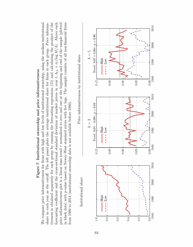
Fig

ure

7.

Inst

ituti

onal

ow

ners

hip

and

pri

cein

form

ati

veness

We

com

par

epri

cein

form

ativ

enes

sfo

rfirm

sw

ith

hig

han

dlo

wle

vels

ofin

stit

uti

onal

owner

ship

,usi

ng

the

med

ian

inst

ituti

onal

shar

ein

each

year

asth

ecu

toff

.T

he

left

pan

elplo

tsth

eav

erag

ein

stit

uti

onal

shar

efo

rfirm

sin

each

grou

p.

Pri

cein

form

a-ti

venes

sis

obta

ined

separ

atel

yfo

rea

chgr

oup

by

runnin

gth

efo

reca

stin

gre

gres

sion

s(1

5)an

dca

lcula

ting

the

pro

duct

ofth

efo

reca

stin

gco

effici

ent

and

the

cros

s-se

ctio

nal

stan

dar

ddev

iati

onof

mar

ket

pri

ces

inye

art,b t,h×σt(l

ogM/A

).A

bov

eea

chpri

cein

form

ativ

enes

splo

tis

alinea

rti

me

tren

dτ

nor

mal

ized

toze

roan

don

eat

the

beg

innin

gan

den

dof

the

sam

ple

(plo

tted

inbla

ckdot

s)w

ithp-

valu

ebas

edon

New

ey-W

est

stan

dar

der

rors

wit

hfive

lags

.T

he

sam

ple

consi

sts

ofal

lnon

-finan

cial

firm

sfr

om19

80to

2014

(inst

ituti

onal

owner

ship

dat

ais

not

avai

lable

bef

ore

1980

).

Inst

ituti

onal

shar

eP

rice

info

rmat

iven

ess

by

inst

ituti

onal

shar

e

h=

3h

=5

64

Figure 8. Option trading and price informativeness

We compare price informativeness for firms with and without option listings and for firmswith high and low option turnover, using median option turnover in each year as the cutoff.Option turnover is 100× option volume over a year divided by equity shares outstanding.Price informativeness is obtained separately for each group by running the forecasting regres-sions (15) and calculating the product of the forecasting coefficient and the cross-sectionalstandard deviation of market prices in year t, bt,h×σt (logM/A). Above each plot is a lineartime trend τ normalized to zero and one at the beginning and end of the sample (plotted inblack dots) with p-value based on Newey-West standard errors with five lags. The sampleconsists of S&P 500 non-financial firms from 1973 to 2014 for the option listing test (theCBOE began listing firms in 1973) and from 1997 to 2014 for the option turnover test (optionvolume is from OptionMetrics, which begins coverage in 1996).

Price informativeness by option listings (1973–2010)

h = 3 h = 5

Price informativeness by option turnover (1997–2010)

h = 3 h = 5

65

Fig

ure

9.

Liq

uid

ity

and

pri

cein

form

ati

veness

We

com

par

epri

cein

form

ativ

enes

sfo

rfirm

sw

ith

hig

han

dlo

wle

vels

ofsh

are

turn

over

,usi

ng

the

med

ian

turn

over

inea

chye

aras

the

cuto

ff.

The

left

pan

elplo

tsth

eav

erag

elo

gtu

rnov

erfo

rfirm

sin

each

grou

p.

Pri

cein

form

ativ

enes

sis

obta

ined

separ

atel

yfo

rea

chgr

oup

by

runnin

gth

efo

reca

stin

gre

gres

sion

s(1

6)an

dca

lcula

ting

the

pro

duct

ofth

efo

reca

stin

gco

effici

ent

and

the

cros

s-se

ctio

nal

stan

dar

ddev

iati

onof

mar

ket

pri

ces

inye

art,b t,h×σt(l

ogM/A

).A

bov

eea

chpri

cein

form

ativ

enes

splo

tis

alinea

rti

me

tren

dτ

nor

mal

ized

toze

roan

don

eat

the

beg

innin

gan

den

dof

the

sam

ple

(plo

tted

inbla

ckdot

s)w

ithp-

valu

ebas

edon

New

ey-W

est

stan

dar

der

rors

wit

hfive

lags

.T

he

sam

ple

consi

sts

ofS&

P50

0non

-finan

cial

firm

sfr

om19

60to

2014

.

Log

turn

over

Pri

cein

form

ativ

enes

sby

turn

over

h=

3h

=5

66

Figure 10. Growth options and price informativeness

We compare price informativeness for firms with high and low valuation ratios, using themedian value of the valuation ratio logM/A in each year as the cutoff. We refer to high-valuation firms as growth firms and low-valuation firms as value firms. Price informativenessis obtained separately for each group by running the forecasting regressions (15) and calcu-lating the product of the forecasting coefficient and the cross-sectional standard deviationof market prices in year t, bt,h × σt (logM/A). Above each plot is a linear time trend τnormalized to zero and one at the beginning and end of the sample (plotted in black dots)with p-value based on Newey-West standard errors with five lags. The sample consists ofS&P 500 non-financial firms from 1960 to 2014.

Price informativeness by level of valuation

Low valuation (value firms) High valuation (growth firms)

67

Figure A.1. Average cross-sectional coefficients by horizon and sub-sample

This figure shows average coefficients calculated from the cross-sectional forecasting regres-sions (15):

Ei,t+h/Ai,t = at,h + bt,h log (Mi,t/Ai,t) + ct,h (Ei,t/Ai,t) + dst,h1si,t + εi,t,h,

where M is market cap, A is total assets, E is earnings (EBIT), and 1s is a sector (one-digitSIC code) indicator variable. We run a separate regression for each year t = 1960, . . . , 2014and horizon h = 1, . . . , 5. We report average of the coefficients bt,h for prices and ct,h forearnings. The horizontal axis represents horizon h. The solid red line shows coefficients athorizon h averaged over the full sample, i.e. 1

55

∑2014t=1960 bt,h and 1

55

∑2014t=1960 ct,h. The dashed

black line is for the first half, 1960 to 1985, and the dash-dotted blue line is for the secondhalf, 1986 to 2014. The sample consists of S&P 500 non-financial firms from 1960 to 2014.

Coefficients on prices bt,h Coefficients on earnings ct,h

68

Fig

ure

A.2

.P

rice

info

rmati

veness

,ro

bust

ness

We

rep

ort

pri

cein

form

ativ

enes

sunder

seve

ral

vari

atio

ns.

Pri

cein

form

ativ

enes

sis

calc

ula

ted

by

runnin

gth

efo

reca

stin

gre

gres

-si

ons

(15)

and

takin

gth

epro

duct

ofth

efo

reca

stin

gco

effici

ent

and

the

cros

s-se

ctio

nal

stan

dar

ddev

iati

onof

mar

ket

pri

ces

inye

art,b t,h×σt(l

ogM/A

).In

the

firs

tco

lum

n,

we

add

the

book

valu

eof

deb

tin

calc

ula

ting

the

valu

atio

nra

tio

(that

isw

euse

M+D

inst

ead

ofM

).In

the

seco

nd

colu

mn,

we

use

EB

ITD

Ain

stea

dof

EB

ITto

mea

sure

earn

ings

.In

the

thir

dan

dfo

urt

hco

lum

ns

we

use

net

inco

me

and

cash

flow

from

oper

atio

ns

(CF

O).

Ab

ove

each

plo

tis

alinea

rti

me

tren

dτ

nor

mal

ized

toze

roan

don

eat

the

beg

innin

gan

den

dof

the

sam

ple

(plo

tted

inbla

ckdot

s)w

ithp-

valu

ebas

edon

New

ey-W

est

stan

dar

der

rors

wit

hfive

lags

.T

he

sam

ple

consi

sts

ofS&

P50

0non

-finan

cial

firm

sfr

om19

60to

2014

.

Adju

stin

gfo

rdeb

tE

BIT

DA

Net

inco

me

Cas

hflow

from

oper

atio

ns

69

Figure A.3. Price informativeness, all firms

Earnings dispersion σt (E/A), valuation dispersion σt (logM/A), coefficients bt,h, and priceinformativeness bt,h × σt (logM/A) from the forecasting regressions (15), run separately forS&P 500 firms and all firms between 1960 and 2014. Above each of the bottom four plotsis a linear time trend τ normalized to zero and one at the beginning and end of the sample(plotted in black dots) with p-value based on Newey-West standard errors with five lags.The dispersion series are measured as the cross-sectional standard deviations in each year.

Earnings dispersion σt (E/A) Valuation dispersion σt (logM/A)

Coefficients bt,h

h = 3 h = 5

Price informativeness bt,h × σt (logM/A)

h = 3 h = 5

70