Embed Size (px)
Citation preview

Harvey, Thomas (2009) Noise in a dynamical open quantum system: coupling a resonator to an artificial atom. PhD thesis, University of Nottingham.
Access from the University of Nottingham repository: http://eprints.nottingham.ac.uk/10829/1/Thomas_Harvey_thesis.pdf
Copyright and reuse:
The Nottingham ePrints service makes this work by researchers of the University of Nottingham available open access under the following conditions.
This article is made available under the University of Nottingham End User licence and may be reused according to the conditions of the licence. For more details see: http://eprints.nottingham.ac.uk/end_user_agreement.pdf
For more information, please contact [email protected]

Noise in a Dynamical Open Quantum
System: Coupling a Resonator to an
Artificial Atom
by Thomas Harvey
Thesis submitted to the University of Nottingham
for the degree of Doctor of Philosophy, April 2009

Abstract
The subject of this thesis is the study of a particular open quantum system consisting
of a resonator coupled to a superconducting single electrontransistor (SSET). The the-
oretical model we use is applicable to both mechanical and superconducting stripline
resonators leading to a large parameter regime that can be explored. The SSET is tuned
to the Josephson quasi-particle resonance, in which the transport occurs via Cooper
pairs coherently tunnelling across one junction followed by the incoherent tunnelling
of quasi-particles across the other. The SSET can be thoughtof as an artificial atom
since it has a similar energy level structure and transitions to an atom. We investigate
to what extent the current and current noise through the SSETcan be used to infer the
state of the resonator. In order to carry out these investigations we describe the system
with a Born-Markov master equation, which we solve numerically. The evolution of
the density matrix of the system is described by a Liouvillian superoperator. In order to
better understand the results we perform an eigenfunction expansion of the Liouvillian,
which is useful in connecting the behaviour of the resonatorto the current noise. The
mixture of coherent and incoherent processes in the SSET leads to interesting back ac-
tion effects on the resonator. For weak coupling the SSET acts as an effective thermal
bath on the resonator. Depending on the operating point the resonator can be either
heated or cooled in comparison to its surroundings. In this regime we can use a set
of mean field equations to describe the system and also capture certain aspects of the
behaviour with some simple models. For sufficient coupling the SSET can drive the
resonator into states of self-sustained oscillations. At the transition between stable and
oscillating states of the resonator we also find regions of co-existence between oscillat-
ing and fixed point states of the resonator. The current noiseprovides a way to identify
these transitions and the state of the resonator. The systemalso shows analogies with
quantum optical systems such as the micromaser. We calculate the linewidth of the
resonator and find deviations from the expected behaviour.
i

Acknowledgements
I would like to thank my supervisor Andrew Armour. Without his help and support
this PhD would not have been possible. Also Denzil Rodrigueshas been like a second
supervisor and I have enjoyed working with them both.
I also want to thank Jane for giving me support home, where I have a life outside
of physics. Finally I would like to thank my fellow PhD students who have made the
last few years so enjoyable.
ii

Contents
Abstract i
Acknowledgements ii
Contents iii
List of Figures v
1 Introduction 11.1 Outline . . . . . . . . . . . . . . . . . . . . . . . . . . . . . . . . . 5
2 SSET and Resonator System 72.1 The single electron transistor. . . . . . . . . . . . . . . . . . . . . . 72.2 The superconducting single electron transistor. . . . . . . . . . . . . 9
2.2.1 Current Processes. . . . . . . . . . . . . . . . . . . . . . . . 102.2.2 Model of a SSET at the JQP resonance. . . . . . . . . . . . 15
2.3 Coupling a resonator to a SET. . . . . . . . . . . . . . . . . . . . . 182.4 Master equation description of the coupled system. . . . . . . . . . . 202.5 Liouville space and the steady state solution of the master equation. . 222.6 Formalism for calculating the noise spectrum of a pair ofoperators. . 232.7 Calculating the current noise of a SSET at the JQP resonance . . . . . 26
3 Signatures of the Dynamical State of the Resonator 293.1 Determining the dynamical state of the resonator. . . . . . . . . . . 293.2 Current and current noise of a SSET. . . . . . . . . . . . . . . . . . 323.3 Frequency regimes of operation. . . . . . . . . . . . . . . . . . . . 323.4 High frequency resonatorΩ ≫ Γ . . . . . . . . . . . . . . . . . . . . 363.5 Low frequency resonatorΩ ≪ Γ . . . . . . . . . . . . . . . . . . . . 403.6 Strongly interacting regimeΩ ∼ Γ . . . . . . . . . . . . . . . . . . . 433.7 Analogy with a micromaser. . . . . . . . . . . . . . . . . . . . . . . 44
4 Resonator in a Thermal State 504.1 SSET as an effective thermal bath. . . . . . . . . . . . . . . . . . . 504.2 Fluctuating gate model. . . . . . . . . . . . . . . . . . . . . . . . . 544.3 Mean field equations. . . . . . . . . . . . . . . . . . . . . . . . . . 564.4 Simple model of the resonator contribution to the current noise . . . . 634.5 Finite frequency current noise in the thermal state. . . . . . . . . . . 66
iii

5 Transitions in the Dynamical State of the Resonator 735.1 A review of the behaviour of the system for moderate coupling . . . . 735.2 A model of a generic bistable system. . . . . . . . . . . . . . . . . . 775.3 Proving the presence of a bistability. . . . . . . . . . . . . . . . . . 785.4 Quantum trajectories. . . . . . . . . . . . . . . . . . . . . . . . . . 805.5 Transitions and time-scales. . . . . . . . . . . . . . . . . . . . . . . 85
6 Finite Frequency Resonator Noise Spectra 936.1 Calculation of the resonator linewidth. . . . . . . . . . . . . . . . . 936.2 Phase Diffusion forΩ ≫ Γ . . . . . . . . . . . . . . . . . . . . . . . 966.3 Phase Diffusion in theΩ ≃ Γ regime. . . . . . . . . . . . . . . . . . 103
7 Conclusion 107
A Details of the Numerical Method 109
B Quantum Trajectories 111
C Mean Field Equations 115C.1 Forming a closed set of equations. . . . . . . . . . . . . . . . . . . 116C.2 Current noise. . . . . . . . . . . . . . . . . . . . . . . . . . . . . . 117
D Calculation of Sx,x(ω) and Sx2,x2(ω) 122
E Adding Qubit Dephasing 125
Bibliography 129
iv

List of Figures
1.1 Images of experimental NEMS. . . . . . . . . . . . . . . . . . . . . 21.2 Images of superconducting resonators coupled to electronic devices . 4
2.1 Schematic diagram of a SET. . . . . . . . . . . . . . . . . . . . . . 82.2 Coulomb diamonds. . . . . . . . . . . . . . . . . . . . . . . . . . . 102.3 Cooper pair resonance lines. . . . . . . . . . . . . . . . . . . . . . . 122.4 Double Josephson quasi-particle cycle. . . . . . . . . . . . . . . . . 132.5 Josephson quasi-particle cycle. . . . . . . . . . . . . . . . . . . . . 142.6 Γ21, Γ10 for varyingVds and〈I〉 not sensitive to different rates.. . . . 17
3.1 Resonator states – Wigner distributions. . . . . . . . . . . . . . . . 303.2 Resonator states –P (n) distributions. . . . . . . . . . . . . . . . . . 313.3 〈I〉 andFI(0) of a SSET . . . . . . . . . . . . . . . . . . . . . . . . 333.4 〈n〉 as a function of∆E andΩ . . . . . . . . . . . . . . . . . . . . . 343.5 Fn as a function of∆E andΩ . . . . . . . . . . . . . . . . . . . . . 353.6 〈I〉 as a function of∆E andΩ . . . . . . . . . . . . . . . . . . . . . 353.7 Current Fano factor,FI(0), as a function of∆E andΩ . . . . . . . . 363.8 〈n〉, Fn, 〈I〉 andFI(0) as a function of∆E andκ for Ω ≫ Γ . . . . . 383.9 P (n) distribution for a continuous transition. . . . . . . . . . . . . . 393.10 〈I〉 / 〈n〉 as a function of∆E andκ for Ω ≫ Γ . . . . . . . . . . . . 393.11 〈n〉 as a function of∆E andκ for Ω ≪ Γ . . . . . . . . . . . . . . . 413.12 〈I〉 as a function of∆E andκ for Ω ≪ Γ . . . . . . . . . . . . . . . 413.13 Fn as a function of∆E andκ for Ω ≪ Γ . . . . . . . . . . . . . . . 423.14 FI(0) as a function of∆E andκ for Ω ≪ Γ . . . . . . . . . . . . . . 423.15 〈n〉 as a function of∆E andκ for Ω ∼ Γ . . . . . . . . . . . . . . . 433.16 〈I〉 as a function of∆E andκ for Ω ∼ Γ . . . . . . . . . . . . . . . 443.17 Fn as a function of∆E andκ for Ω ∼ Γ . . . . . . . . . . . . . . . . 453.18 FI(0) as a function of∆E andκ for Ω ∼ Γ . . . . . . . . . . . . . . 453.19 〈n〉 as a function ofκ for 3 values ofγext . . . . . . . . . . . . . . . 473.20 Fn as a function ofκ for 3 values ofγext . . . . . . . . . . . . . . . . 473.21 ChangingP (n) distribution with increasingκ for smallγext . . . . . 483.22 ChangingP (n) distribution with increasingκ for largeγext . . . . . . 48
4.1 γSSET andnSSET . . . . . . . . . . . . . . . . . . . . . . . . . . . . 524.2 〈I〉 for thermal state resonator. . . . . . . . . . . . . . . . . . . . . 534.3 FI(0) for thermal state resonator. . . . . . . . . . . . . . . . . . . . 534.4 Comparison of
⟨
x2⟩
values . . . . . . . . . . . . . . . . . . . . . . . 584.5 FI(0) for thermal state resonator and very smallκ . . . . . . . . . . . 614.6 Eigenvalue contributions toFI(0) . . . . . . . . . . . . . . . . . . . 62
v

4.7 Fit of eigenvalue contributions to model. . . . . . . . . . . . . . . . 664.8 Current noise spectrum for thermal state. . . . . . . . . . . . . . . . 684.9 Lorentzian fit toω = 0 peak . . . . . . . . . . . . . . . . . . . . . . 694.10 FI(ω) peak atω = 0 for varying∆E . . . . . . . . . . . . . . . . . 694.11 ω = ΩR peak for increasingnext . . . . . . . . . . . . . . . . . . . . 704.12 FI(ω) peak atω = ΩR for varying∆E . . . . . . . . . . . . . . . . 714.13 FI(ω) peak atω = 2ΩR for varying∆E . . . . . . . . . . . . . . . . 724.14 FI(ω) peak atω = 2ΩR comparison of simple model and mean field. 72
5.1 Current for varying∆E in three frequency regimes. . . . . . . . . . 745.2 FI(0) for Ω = 0.12 Γ with approximations. . . . . . . . . . . . . . . 755.3 FI(0) for Ω = Γ with approximations . . . . . . . . . . . . . . . . . 765.4 FI(0) for Ω = 10 Γ with approximations. . . . . . . . . . . . . . . . 765.5 Proof of bistability using〈〈I3〉〉 and peak inSI,I(ω) . . . . . . . . . . 795.6 Quantum trajectories. . . . . . . . . . . . . . . . . . . . . . . . . . 825.7 Quantum trajectory of〈n〉t andP (n) distribution for a bistable system 845.8 First few real eigenvalues forΩ = 0.12 Γ . . . . . . . . . . . . . . . 875.9 Fn and approximations forΩ = 0.12 Γ . . . . . . . . . . . . . . . . . 875.10 Variance part of current noise forΩ = 0.12 Γ . . . . . . . . . . . . . 895.11 Fn and approximations forΩ = Γ . . . . . . . . . . . . . . . . . . . 905.12 First few real eigenvalues forΩ = Γ . . . . . . . . . . . . . . . . . . 905.13 First few terms in
⟨
n2⟩
expansion forΩ = Γ . . . . . . . . . . . . . . 915.14 Fn and approximations forΩ = 10 Γ . . . . . . . . . . . . . . . . . . 925.15 First few real eigenvalues forΩ = 10 Γ . . . . . . . . . . . . . . . . 92
6.1 Saa†(ω)and〈n〉Spp†(ω) for ω ≃ Ω in the limit cycle region . . . . . 956.2 Use of eigenvalues to give width of finite frequency spectra . . . . . . 976.3 〈n〉, m1
e andm1p as a function of∆E for Ω = 10 Γ . . . . . . . . . . 98
6.4 γn and real part of two eigenvalues nearest−iΩ . . . . . . . . . . . . 996.5 〈n〉 as a function ofκ andγext . . . . . . . . . . . . . . . . . . . . . 1006.6 −ℜλΩ as a function ofκ andγext . . . . . . . . . . . . . . . . . . . 1006.7 〈n〉 for varying∆E andκ . . . . . . . . . . . . . . . . . . . . . . . 1016.8 Fn for varying∆E andκ . . . . . . . . . . . . . . . . . . . . . . . . 1026.9 γΩ for varying∆E andκ . . . . . . . . . . . . . . . . . . . . . . . . 1026.10 Height of peak in emission spectrum. . . . . . . . . . . . . . . . . . 1036.11 γn for varying∆E andκ . . . . . . . . . . . . . . . . . . . . . . . . 1046.12 FI(0) for varying∆E andκ . . . . . . . . . . . . . . . . . . . . . . 1046.13 〈n〉, m1
e andm1p as a function of∆E for Ω = Γ . . . . . . . . . . . . 105
6.14 −ℜλp for −iΩ eigenvalues. . . . . . . . . . . . . . . . . . . . . . . 106
E.1 Comparison of current with experiment. . . . . . . . . . . . . . . . 127
vi

Chapter 1
Introduction
There is always a desire to scale down devices to ever smallerscales. An example, of
relevance to this thesis, is electromechanical systems, which consist of an electronic
device coupled to a mechanical degree of freedom. The first such device is thought to
be Coulomb’s electrical torsion balance in 1785 [1]. The idea of an electromechanical
system is simply to act as a transducer, converting mechanical motion into a measurable
electrical signal or conversely to convert an applied electrical signal into mechanical
motion.
Devices at the micron-scale are known as microelectromechanical systems (MEMS).
MEMS devices are common place and find applications in tiny moveable mirrors in
digital projectors, motion sensors for car air bags, video game controllers and micro-
biology [1–3]. With the great successes of devices at the micron-scale the natural
continuation is to the nano-scale and the creation of nanoelectromechanical systems
(NEMS) [1, 2, 4–6].
At the nano-scale the mechanical part may be, a carbon nanotube [7], a small pil-
lar [8], a cantilever [9] or a beam [10]. In figure1.1we show some examples of a few
of these devices. The device in figure1.1ais a shuttle device [8]. An ac voltage is
applied to the pillar (labelled I) via the source and drain electrodes (labelled S and D).
When the pillar is driven at the correct frequency an enhancement of the current is seen
corresponding to electrons tunnelling onto the pillar whennear the source electrode
and off again when near the drain electrode. Devices of this kind may see applications
as a mechanical switch [8].
In this thesis we are interested in devices of the type shown in figure1.1c [10].
This consists of a single electron transistor (SET) [11, 12] where a freely suspended
beam is capacitively coupled to the island (see Section2.3). The current through the
device is sensitive to the position of the beam and so could see applications in position
detection [13].
Due to the small size of the mechanical parts they have very high fundamental
1

Figure 1.1. (a) Transistor with the island formed from from a nanome-chanical pillar reproduced from [8]a. (b) Suspended carbon nanotubeforming the island of a transistor reproduced from [7]b. (c) Single elec-tron transistor where one of the plates of the gate capacitoris a doublyclamped beam, reproduced from [10]c. The scale bar shows 1µm
aReprinted from Superlattices and Microstructures,33, R. H. Blick and D. V. Scheible, A quantum elec-tromechanical device: the electromechanical single-electron pillar, p397, copyright (2003), with permissionfrom Elsevier
bReprinted by permission from Macmillan Publishers Ltd: Nature (431284), copyright (2004)cReprinted by permission from Macmillan Publishers Ltd: Nature (424291), copyright (2003)
2

frequencies, of the order 10Hz–1GHz. At these frequencies the device can be suffi-
ciently cooled, in a dilution fridge, that the thermal fluctuations in energy of the beam,
kBT , are less than the spacing between energy states of a quantumharmonic oscillator,
~Ω [6]. This suggests that a quantum mechanical description is necessary for these de-
vices and that in the future it should be possible to observe interesting quantum effects
in NEMS [6].
At the nano-scale charging effects cannot be neglected whenconsidering metallic
objects [11]. These lead to discrete energy levels in the metallic island at the centre
of the SET. The device we consider in this thesis is a superconducting SET (SSET),
so Cooper pairs as well as quasi-particle excitations take part in the transport through
the system, which leads to resonances in the current (see Section 2.2). We focus on a
particular resonance known as the Josephson quasi-particle (JQP) resonance [14–17],
where Cooper pair tunnelling takes place at one junction andquasi-particle tunnelling
at the other. Theoretical investigations of the SSET-resonator system at this resonance
have led to predictions of a range of interesting effects of the SSET on the resonator
including cooling, driving into states of self-sustained oscillations and the formation
of non-classical states [18–24]. Experimental efforts have so far have focused on cool-
ing [21] and position detection [25].
Although an interesting field of study NEMS have yet to unambiguously show
quantum behaviour [26–28]. However, the theoretical methods we use can equally be
applied to other systems where a SSET couples to a harmonic mode. Superconduct-
ing stripline resonators support harmonic modes that at dilution fridge temperatures are
almost unaffected by thermal noise. The strong coupling of electronic devices to super-
conducting stripline resonators has also been an area of active research experimentally,
first with qubits [29], and more recently with a SSET at the JQP resonance [30], ex-
amples of which are shown in figure1.2. It is thought that a superconducting stripline
resonator could provide a bus between qubits in a quantum computer [31].
Electronic devices such as the SSET are often known as artificial atoms. This is
because the energy level structure and transitions that occur in the solid state devices
are similar to those in atoms. We can therefore use many techniques and ideas from
quantum optics to investigate our device. The SSET interacting with a resonator shows
many similarities with an atom interacting with a light field. In later chapters of this
thesis we make some comparisons between features we find and those seen in quantum
optical systems.
In a realistic model of any device it is important to take account of the surroundings
of the system we are interested in. Within a quantum formulation this field is known as
open quantum systems [32, 33]. Interaction with the environment leads to dissipation
and can destroy the quantum nature of the device. However, interaction with the en-
vironment is also essential to perform measurements on the system, for instance there
would be no dc current at the JQP resonance without dissipation.
3

Figure 1.2. (a–c) False colour image of a qubit coupled to a supercon-ducting stripline resonator reproduced from [29]a. (a) Green regions arethe silicon substrate and beige the central conductor and ground planesforming the cavity. (b) An expansion of one of the capacitorsat the endof the cavity. (c) The qubit is shown in blue fabricated in thegap betweenthe central conductor and ground plane. (d,e) Superconducting striplineresonator coupled to a SSET, reproduced from [30]b. (d) Micrograph ofone end of the resonator showing an aluminium strip that extends from themiddle of the resonator to the SSET. (e) Scanning electron micrograph ofthe SSET.
aReprinted by permission from Macmillan Publishers Ltd: Nature (431162), copyright (2004)bReprinted by permission from Macmillan Publishers Ltd: Nature (449588), copyright (2007)
4

1.1. Outline
Experimentally the state of the resonator is not directly accessible. The state must
be inferred, either from measurements performed on the SSETor, for the case of the
superconducting stripline resonator, emission from the cavity can be measured. As we
show later the current through the SSET is only sensitive to average properties of the
system, but the current noise can be used to reveal information about the dynamics of
the resonator.
1.1 Outline
Chapter2 of this thesis contains the background material and methodsused in the
following chapters to investigate the SSET-resonator system that is the subject of this
thesis. It begins with a discussion of both normal and superconducting single electron
transistors and the transport processes that occur. The coupling of the electronic device
to a resonator is also described along with a discussion of two of the types of resonator
(mechanical and superconducting) that we can consider. Theremainder of the chapter
is devoted to the master equation description of the system and the methods by which
it can be used to calculate the steady-state and noise properties of the device.
Chapter3 begins with a discussion of how the state of the resonator is determined
and the types of dynamical state that occur. The simplest state of the resonator is
the fixed point state, where the resonator is damped by the SSET. For weak coupling
(between the SSET and resonator) the fixed point state is a thermal state, since the
SSET behaves like an effective thermal bath for the resonator. If the system is tuned
so that the SSET gives energy to the resonator during the JQP cycle then, for sufficient
coupling, the resonator is driven into states of self-sustained oscillations, which we
refer to as a limit cycle state. We also observe states where fixed point and limit cycle
states co-exist. An overview of the behaviour for a range of parameters is given in
Chapter3, in order to identify regions of common behaviour. In particular we identify
three frequency regimes of operation corresponding to the resonator being either much
faster, much slower or on the same time-scale as the SSET. Thechapter finishes with a
comparison of the SSET-resonator system and the particularquantum optical device of
a micromaser.
Chapter4 is devoted to an analysis of the regime, in which the resonator remains
in a thermal like state. The current through the SSET can be captured by a very sim-
ple model that assumes that the fluctuations in the position of the resonator cause a
smearing out of the JQP current peak and a shift in the averageposition of the res-
onator causes a shift in the current peak. However, this simple model is not sufficient
to capture the current noise, since it neglects both the dynamics of the resonator and
the correlations between the SSET and resonator. Mean field equations can be used to
describe the system but they do not form a closed set. Due to the Gaussian nature of the
resonator distribution we can form a closed set of equationsby assuming that all third
5

1.1. Outline
order cumulants of the operators used to describe the systemare zero. These equations
provide an accurate description of the system in this regime. We then derive a second
simple model for the current noise that also includes the dynamics of the resonator,
but still neglects correlations between the SSET and resonator. This second model is
valid for a large external temperature or large external damping of the resonator. Fi-
nally we investigate the finite frequency current noise in this regime. It is found that a
combination of the simple models and an eigenfunction expansion of the current noise
expressions can be used to understand the spectrum.
The focus of Chapter5 is the transitions between dynamical states of the resonator
as a function of the parameters. We pay particular attentionto the region where the dy-
namics of the resonator is approximately bistable. In this regime the resonator switches
slowly between two different dynamical states, which are associated with two different
average currents through the SSET. Extensive use is made of an eigenfunction expan-
sion of the current noise in this chapter in order to connect fluctuations in the resonator
to the current noise.
Chapter6 is the final major chapter of the thesis. It is concerned with further laser
analogies that can be explored in the device by focusing on the limit cycle region. For
a laser the rate of phase diffusion is inversely proportional to the energy of the laser
cavity. Although we find this to be true to some extent, calculations of the rate of phase
diffusion for the SSET-resonator system show deviations from the simple relationship
for the laser.
Chapter7 gives the conclusions of the thesis. There are also a number of ap-
pendixes that give further details of various parts of the thesis and in addition a com-
parison with some recent experimental results in AppendixE.
Following Section2.5 and with the exception of Section4.1, the contents of this
thesis are the result of new investigations carried out by the author in collaboration with
Andrew Armour and Denzil Rodrigues. The main publication ofthe results contained
in this thesis is in [24]. This publication focused on the zero frequency current noise
and contained some of the numerical results from Chapter3. In the thermal regime it
included the results from Sections4.2and4.3. Also introduced was the eigenfunction
expansion of the current noise along with most of the resultsof Chapter5. In an
earlier publication, [22], some of the numerical methods as described in Section2.5
and AppendixA were used. The work on phase diffusion described in Chapter6 and
the work on quantum trajectories described in Section5.4will be the subject of future
publications.
6

Chapter 2
SSET and Resonator System
This chapter begins with a discussion of the normal state single electron transistor
as this introduces many of the concepts required to understand the superconducting
device. Section2.2 then looks at a superconducting single electron transistor(SSET)
and describes the resonant transport regimes. In particular the Josephson quasi-particle
(JQP) resonance, which form the focus of this thesis, is discussed in detail. The master
equation for transport at the JQP resonance is also given. Section 2.3 describes the
coupling of a resonator to a single electron transistor. In Section2.4 we give the full
master equation description of the coupled SSET-resonatorsystem. The way in which
the master equation can be solved numerically is described in Section2.5together with
details of the Liouville space description of the system. InSection2.6we introduce a
formalism for calculating the noise spectrum of a pair of operators in a general system.
Finally in Section2.7 we apply this formalism to the SSET at the JQP resonance to
calculate the current noise.
2.1 The single electron transistor
A single electron transistor (SET) [34] consists of a metal island linked to two leads
by two tunnel junctions with capacitancesCL andCR, as shown schematically in fig-
ure2.1. The left and right junctions form the source and drain of thetransistor and a
voltageVds is applied across them. A capacitor,Cg, forms a gate and has a voltageVg
applied to it. The island has a charging energy,Ec, which is the electrostatic energy
required to add an additional electron to the island [11],
Ec =e2
2CT, (2.1.1)
whereCT = CL +CR +Cg is the total capacitance of the island ande = 1.6×10⁻¹⁹C
is the elementary charge. For a large device the charging energy is small and can easily
7

2.1. The single electron transistor
CL CR
Vds
Cg
Vg
Figure 2.1.Schematic diagram of a SET.CL andCR are tunnel junctionsacross which a voltageVds is applied.Cg is the gate capacitor, which hasa voltageVg applied.
be overcome by thermal effects (i.e.Ec ≪ kBT ). For a small island, however, the total
capacitance is small and we can haveEc ≫ kBT , so for an electron to tunnel onto the
island a sufficiently large voltage bias must be applied in order to overcome this energy
cost.
To understand the transport in the device we must consider the energy change of
the system due to the tunnelling of a charge across each of thejunctions. For the device
shown in figure2.1, assuming a positive bias (Vds > 0) and zero temperature so that
electrons only flow from left to right, the relevant energy changes∆EL and∆ER for
a single electron to tunnel across the left and right junctions are [12],
∆EL(n) =e
CT
[
−e
2+ CgVg + Vds
(
CR +1
2Cg
)
− ne
]
= −Ec (2n + 1 − 2ng) + cReVds, (2.1.2)
∆ER(n) =e
CT
[
−e
2− CgVg + Vds
(
CL +1
2Cg
)
+ ne
]
= Ec (2n − 1 − 2ng) + cLeVds, (2.1.3)
wheren is the initial number of excess charges on the island.ng ≡ CgVg
e is the
effective change in the number of charges on the island due tothe applied gate voltage.
cL ≡ 2CL+Cg
2CTandcR ≡ 2CR+Cg
2CTgive the symmetry of the device and always sum
to unity [35, 36]. Tunnelling across the left hand junction changesn → n + 1 and
tunnelling across the right hand junctionn → n − 1. In order for an electron to
tunnel across a junction the energy change, as given by equation 2.1.2or 2.1.3, must
be positive, which corresponds to the system moving to a state of lower energy. The
conditions on the bias that must be applied (for tunnelling in the forward direction) for
8

2.2. The superconducting single electron transistor
each of the two junctions are,
∆EL : cReVds ≥ Ec (2n + 1 − 2ng) , (2.1.4)
∆ER : cLeVds ≥ −Ec (2n − 1 − 2ng) , (2.1.5)
Taking the simple example of an initially neutral island (n = 0), zero gate voltage
(Vg = 0) and symmetric junctions (cL = cR = 12 ). A drain source voltage ofeVds ≥
2Ec is required for an electron to tunnel across either junction. For a second electron to
tunnel across the same junction (and so change the island charge by two) will require
eVds ≥ 6Ec. Further increasingVds allows states with larger numbers of electrons on
the island to be accessed. So long as the tunnelling conditions for one junction are
met the current can flow. The reason being that increasingn, by an electron tunnelling
across the left hand junction, results in a reduction of the energy required to tunnel
across the right hand junction. Similarly decreasingn, by an electron tunnelling across
the right hand junction, reduces the energy requirement fortunnelling across the left
hand junction. The restriction of the allowed charge statesof the island due to charging
effects is known as Coulomb blockade.
A clear signature of these charging effects can be observed experimentally as steps
in the current for increasing drain source voltage known as the Coulomb staircase [37].
In order to observe the Coulomb staircase the junctions should be asymmetric [11].
To achieve this asymmetry we can still use equal capacitances but have the junction
resistances very different. For example if the resistance of the right hand junction is
small then any electrons that tunnel onto the island via the left hand junction can rapidly
tunnel off again through the right hand junction. The current is then controlled by the
ease with which electrons can tunnel across the left hand junction. The result is a jump
in the current when a new island charge state becomes accessible [11].
By tuning the gate voltage the conditions for tunnelling aremodified. For exam-
ple if ng = 1/2 an electron can tunnel from the left lead to the island atVds = 0
and so the blockade is removed entirely. A stability plot, shown in figure2.2, can be
produced showing the regions where the Coulomb blockade restricts the charge state
of the island to a fixed value. Small adjustments in the gate voltage switch the device
from almost no current to a finite value. This allows the device to act as a very sen-
sitive electrometer [38], the sensitivity of which is limited by the temperature of the
device [11].
2.2 The superconducting single electron transistor
Single electron transistors are typically made of Aluminium [34, 38] and so at a low
enough temperature become superconducting. A single electron transistor made en-
tirely from superconducting material and below the transition temperature is known
9

2.2. The superconducting single electron transistor
ng
eVds2Ec
-1 -1/2 1/2 1
1
-1
n=-1 n=0 n=1
Figure 2.2.Coulomb diamonds for a single electron transistor, withcL =cR = 1
2 . Within the diamond shapes the island has a fixed charge (ne) andno current can flow. ForVds > 0 the Coulomb blockade conditions aregiven in equations2.1.4and2.1.5. Equivalent conditions can be found fortransport in the opposite direction (Vds < 0) [11].
as a superconducting single electron transistor (SSET) [39]. In a superconductor the
main charge carriers are Cooper pairs. The tunnelling of Cooper pairs across the junc-
tions is described by the Josephson effect [40]. In order for this tunnelling to occur the
Fermi energies on each side of the junction must be close to alignment. Cooper pair
tunnelling is a resonant process as opposed to the tunnelling of electrons in the SET,
which has a threshold energy requirement.
In bulk superconductor electrons exist as quasi-particle excitations [39]. At a bar-
rier it is the electron that tunnels through, although it exists as a quasi-particle on either
side. We are not concerned with the details of this process here and just refer to the
tunnelling of quasi-particles, see [39] for a detailed treatment.
The combination of the resonant tunnelling of Cooper pairs and incoherent tun-
nelling of quasi-particles leads to a number of different current processes in the SSET.
We discuss some of these in Section2.2.1. In this thesis we focus on a particular one
of these current processes, that of the Josephson quasi-particle (JQP) cycle [14–17]. A
model of which is discussed in Section2.2.2.
2.2.1 Current Processes
In a superconductor a gap in the density of states opens at theFermi energy of width
2∆, where∆ is the superconducting gap. Thus for a quasi-particle (as opposed to
a Cooper pair) to tunnel across a junction between two superconductors requires an
10

2.2. The superconducting single electron transistor
applied bias of at least this energy. For a pair of junctions the energy requirements
calculated for the normal state SET will still hold, but an additional energy of4∆
is required (2∆ for each junction). There is a region of large current above adrain
source voltage of4∆, the border of which shows the Coulomb diamond shape seen in
figure2.2, see for example [41, 42]. The lowest value of the drain-source voltage at
which the quasi-particle current can flow corresponds tong = 12 .
Other features occur for lower bias voltages than that required for pure quasi-
particle current to flow. These are resonances involving thetransport of Cooper pairs in
the system, which is described by Josephson tunnelling [40, 43]. The following Hamil-
tonian can be used to describe the Cooper pair tunnelling across one of the junctions,
between the states withn andn + 2 excess charges on the island [43],
Hcp = ∆En,n+2 |n + 2〉〈n + 2| − EJ
2
(
|n〉〈n + 2| + |n + 2〉〈n|)
, (2.2.1)
whereEJ is the Josephson coupling energy between the two superconductors and
∆En,n+2 is the electrostatic energy difference between the two charge states. Typi-
cally,EJ and∆En,n+2 will be different for each of the two junctions. Evolution under
the Hamiltonian describes an oscillation between then andn + 2 charge states of the
island, which corresponds to an AC current across the junction. When∆En,n+2 = 0
the eigenstates of the Hamiltonian consist of a superposition of equal amounts of the
two charge states, which corresponds to the resonant tunnelling of Cooper pairs.
For the left hand junction,∆ELn,n+2 can be calculated by using equation2.1.2,
which gives the energy to add an electron to the island.∆ELn,n+2 will be the energy
required to add two electrons onto the island of the SET separately, across the left hand
junction,
∆ELn,n+2 = ∆EL(n) + ∆EL(n + 1) = −4Ec (n + 1 − ng) + 2cReVds. (2.2.2)
For the right hand junction equation2.1.3gave the energy to remove an electron from
the island across the right hand junction and so∆ERn,n+2 is,
∆ERn,n+2 = ∆ER(n + 2) + ∆ER(n + 1) = 4Ec (n + 1 − ng) + 2cLeVds. (2.2.3)
The Cooper pair resonance conditions are satisfied for linesin the Vg–Vds plane for
different values of the initial island charge,ne, as shown in figure2.3.
Cooper pair tunnelling alone will not lead to a DC current here. It is necessary
to also have tunnelling of quasi-particles. AteVds = 2Ec, as indicated in figure2.3,
there is a crossing between the Cooper pair resonance lines differing by n = 1. At this
crossing a particular current resonance known as the doubleJosephson quasi-particle
(DJQP) or3e resonance occurs [44]. At the DJQP resonance only one junction is
close to resonance for Cooper pair tunnelling at any one time. The current flows in
11

2.2. The superconducting single electron transistor
−0.1 −0.05 0 0.05 0.10
0.2
0.4
0.6
0.8
1
x 10−3
Vg (V )
Vds(m
V)
4Ec/e
2Ec/e
2∆+ Ec/e
n=-4n=-3n=-2n=-1n=0n=1
Figure 2.3. The lines indicate the positions of Cooper pair resonances intheVg–Vds plane, as given by equations2.2.2and2.2.3. The resonancesoccur between the charge statesn andn + 2. The parameters used aretaken from the experiment in [42], CL = 210 aF, CR = 117 aF, Cg =3.15 aF, Ec = 240 µeV and∆ = 198 µeV. Note that the system has anegative bias applied in [42] and there is a shift in the gate voltage dueto background charges that is not included here. Also indicated are theJQP cycle threshold (2∆+Ec), the position of the DJQP resonance (2Ec)and the crossing point of the JQP resonances with the same island charge(4Ec).
12

2.2. The superconducting single electron transistor
0 2
1-1Figure 2.4.Double Josephson quasi-particle cycle (DJQP).|−1〉, |0〉, |1〉and|2〉 correspond to−1, 0, 1 and2 excess electrons on the island.
the following cycle, which is shown in figure2.4. First one junction is on resonance
for Cooper tunnelling. A quasi-particle then tunnels across the second junction, which
switches the Cooper pair resonance to the second junction. Asecond quasi-particle
tunnelling across the first junction then switches the system back to the initial state of
the Cooper pair resonance at the first junction. It is known asthe3e resonance as three
electrons are transported through the SSET during the cycle.
In this thesis we are going to study the Josephson quasi-particle (JQP) resonance [14–
17]. For this resonance Cooper pair tunnelling is close to resonance at only one junc-
tion. For a sufficiently large drain source voltage two quasi-particles can tunnel se-
quentially across the other junction. Taken together the Cooper pair and quasi-particle
tunnelling lead to a cycle, in which 2 charges are transferred through the SSET. The
cycle is shown schematically in figure2.5 for Cooper pair tunnelling at the left hand
junction.
In addition to being near a resonance for Cooper pair tunnelling the JQP reso-
nance requires that the tunnelling of the two quasi-particles is energetically favourable.
Throughout this thesis we choose the left hand junction to beclose to the Cooper pair
resonance and consider quasi-particle tunnelling only at the right hand junction, al-
though the results would be equally valid for the reverse case. The energy require-
ments for the quasi-particle tunnelling can be calculated from equation2.1.3with an
additional penalty of2∆ due to the superconducting gap. For an initial island charge
of ne, and following the tunnelling of a Cooper pair onto the island across the left hand
junction there will ben + 2 excess electrons on the island. The energy changes for the
two quasi-particles to tunnel across the right-hand junction and return the island to the
13

2.2. The superconducting single electron transistor
0 2
1Figure 2.5.The JQP cycle, Cooper pairs tunnel across the left hand junc-tion, which is interrupted by the splitting of the Cooper pair and the tun-nelling of two quasi-particles through the right hand junction. |0〉, |1〉 and|2〉 correspond to zero, one or two electrons on the island.
n state are,
∆ER(n + 2) − 2∆ = Ec (2n + 3 − 2ng) + cLeVds − 2∆, (2.2.4)
∆ER(n + 1) − 2∆ = Ec (2n + 1 − 2ng) + cLeVds − 2∆. (2.2.5)
As before these changes must be positive. The second quasi-particle tunnelling requires
the higher voltage so as long as this condition is satisfied the first will also be satisfied.
For the JQP resonance there are two conditions that need to bemet,
cReVds ≃ 2Ec (n + 1 − ng) , (2.2.6)
eVds ≥ Ec + 2∆. (2.2.7)
The first is the condition for the Cooper pair resonance at theleft hand junction and
the second is the threshold voltage for quasi-particle tunnelling whenon resonance,
which is found by combining equations2.2.5and2.2.6. Notice that the threshold is
independent of the island charge, gate charge and capacitances and is indicated on
figure2.3.
Other processes such as Andreev reflection [45] can also be observed in this system.
Throughout this thesis we assume that only the conditions for the JQP resonance are
met and ignore all other transport processes.
There are several advantages of the JQP resonance that aid its experimental inves-
tigation. The cycle is periodic ine so unlike the supercurrent due to Cooper pair tun-
nelling alone it is not affected by quasi-particle poisoning, where an unwanted quasi-
particle tunnels onto the island and blocks the supercurrent [39]. The periodicity also
14

2.2. The superconducting single electron transistor
means that it does not matter what the initial value ofn is. The Cooper pair and quasi-
particle tunnelling occur at different junctions so the parameters for the two processes
can be individually tuned by constructing a very asymmetricdevice. For example the
device in [46] allowed the adjustment of the Josephson coupling energy atone junc-
tion by applying a magnetic field. A high resistance tunnel junction formed the second
junction, so the current could be used as a probe of the strongJosephson tunnelling.
2.2.2 Model of a SSET at the JQP resonance
A full master equation description of the SSET tuned to the JQP resonance can be de-
rived from a Hamiltonian for the microscopic degrees of freedom of the system [47].
The Hamiltonian is split into two parts, the system consisting of the island charge and
the reservoir consisting of the unwanted degrees of freedomof the SSET. To obtain
the master equation the reservoir is traced out making Born and Markov approxima-
tions [32, 33, 48]. The approximation made is that correlations in the reservoir decay
fast in comparison to the time scales in the system.
The JQP resonance is periodic in the island charge as is clearfrom equation2.2.6
and figure2.3. We label the states for an initially neutral island for simplicity, and
so consider just the three charge states|0〉, |1〉 and|2〉. As mentioned previously we
choose the Cooper pair tunnelling to be at the left hand junction. From equation2.2.1
the Hamiltonian for the Cooper pair tunnelling part of the evolution is,
HSSET = ∆E |2〉〈2| + EJ
2(|0〉〈2| + |2〉〈0|) (2.2.8)
where∆E ≡ ∆EL0,2 = −4Ec(1 − ng) + 2cReVds, is the detuning from the Cooper
pair resonance (equation2.2.2) andEJ is the Josephson coupling energy for the left
hand junction. This Hamiltonian describes an effective qubit between the zero and two
charge states. The evolution of the system is given by the master equation [17],
ρ(t) = − i
~[HSSET, ρ(t)] + Lqpρ(t), (2.2.9)
whereρ(t) is the reduced density matrix of the system [33], describing just the three
charge states andLqp is a superoperator describing the quasi-particle tunnelling. We
will come back to a full description of superoperators in Section 2.5.
The quasi-particle part of the evolution is dissipative andcauses decoherence of the
qubit. It must include the two quasi-particle decays to takethe system from the|2〉
15

2.2. The superconducting single electron transistor
state back to the|0〉 state incoherently. The quasi-particle term is given by [16, 22],
Lqpρ(t) = Γ21
[
|1〉〈2| ρ(t) |2〉〈1| − 1
2|2〉〈2| , ρ(t)
]
+ Γ10
[
|0〉〈1| ρ(t) |1〉〈0| − 1
2|1〉〈1| , ρ(t)
]
+Γ21 + Γ10
2
[
|1〉〈2| ρ(t) |1〉〈0| + |0〉〈1| ρ(t) |2〉〈1|]
, (2.2.10)
whereΓ21, Γ10 are the tunnelling rates for the two processes and· , · is the anti-
commutator. The terms on the first two lines describe the quasi-particle decays from
|2〉 → |1〉 and|1〉 → |0〉 respectively and are of Lindblad form [49]. The final term is
often omitted (e.g. [47]). It describes part of the evolution of the off-diagonal density
matrix elements corresponding to the coherence between the|1〉 state and the other two
charge states. Since the Hamiltonian (equation2.2.8) does not generate any coherence
between the|1〉 state and the|0〉 or |2〉 states these elements rapidly decay to zero and
have no influence on the dynamics of the rest of the system, as we show below.
The quasi-particle tunnelling rate from left to right through a barrier is [50],
Γ(ε) =1
e2RN
∫ ∞
−∞
dEiL(Ei)f(Ei)R(Ei + ε) [1 − f(Ei + ε)] , (2.2.11)
whereRN is the junction resistance,L(R)(Ei) are the normalized density of states on
the left (right) of the barrier,ε is the electrostatic energy change of the system (given
by equation2.1.3) andf(Ei) is the Fermi function,
f(Ei) =1
1 + exp (Ei/kBT ). (2.2.12)
For a superconductor the density of states has a gap of width2∆ at the Fermi energy
Ei = 0,
(Ei) =|Ei|
√
E2i − ∆2
Θ (|Ei| − ∆) , (2.2.13)
whereΘ(x) is the Heaviside step function.
Near the JQP resonance the energy changes, for the two transitions, are given by,
ε21 = ∆ER(2) = eVds + Ec −1
2∆E, (2.2.14)
ε10 = ∆ER(1) = eVds − Ec −1
2∆E, (2.2.15)
where we have incorporated the definition of∆E into equation2.1.3. For the quasi-
particle tunnelling rates to be non-zero sufficient voltagemust be applied in order to
overcome the superconducting gap as shown in figure2.6a. For the first quasi-particle
tunnelling the threshold is ateVds = 2∆ − Ec + 12∆E and the second ateVds =
16

2.2. The superconducting single electron transistor
0 0.5 10
10
20
30
40
50
60
Vds (mV)
Γ21,Γ
10
(ns−
1)
(a)
−0.2 −0.1 0 0.1 0.20
0.1
0.2
0.3
0.4
0.5
0.6
0.7
∆E/eVds〈I〉(
nA
)
(b)Γ21
Γ10
exactapprox
Figure 2.6. (a) Tunnelling rates at JQP resonance for varying drain sourcevoltage at zero temperature obtained from a numerical integration of equa-tion 2.2.11. (b) Current at the JQP resonance.exactis the current usingrates calculated from equation2.2.11andapproxis the current assumingthat the rates are given byΓ21 at∆E = 0. Parameters are the same as infigure2.3.
2∆ + Ec + 12∆E. After the threshold is reached the increase in the tunnelling rates
are, to a good approximation, linear and given byΓ21,10 = (eVds ± Ec)/e2RN where
the plus sign is forΓ21 [42].
From the master equation it is straightforward to write downa set of equations for
the SSET island charge and the coherence between the|0〉 and|2〉 charge states. There
are five equations in total for which we use the notationρab(t) ≡ Tr [|a〉〈b| ρ(t)],
ρ00(t) = 1 − ρ11(t) − ρ22(t) (2.2.16)
ρ11(t) = Γ21ρ22(t) − Γ10ρ11(t) (2.2.17)
ρ22(t) = −iEJ
2~(ρ02(t) − ρ20(t)) − Γ21ρ22(t) (2.2.18)
ρ02(t) =
(
−i∆E
~− Γ21
2
)
ρ02(t) + iEJ
2~(ρ00(t) − ρ22(t)) (2.2.19)
ρ20(t) = ρ02(t)† (2.2.20)
Two of the equations have been expressed in terms of the otherthree. This can be done
because of the Hermitian nature of the density matrix (equation2.2.20) and the normal-
isation of the density matrix Tr[ρ(t)] = ρ00(t)+ρ11(t)+ρ22(t) = 1 (equation2.2.16).
Notice also that, as discussed below equation2.2.10, we do not require equations for
ρ10(t), ρ01(t), ρ12(t) or ρ21(t) in order to describe the evolution of the island charge.
The set of equations can be easily solved to find the steady-state probabilities for
17

2.3. Coupling a resonator to a SET
each of the charge states. The current through the SSET at theJQP resonance is
then [14, 51],
〈I〉 = Γ21ρ22(∞) + Γ10ρ11(∞)
=2eE2
JΓ21
4∆E2 + ~2Γ221 + E2
J
(
2 + Γ21
Γ10
) , (2.2.21)
where the∞ indicates that the probabilities are evaluated in the steady-state. In this
thesis we will typically work in the regime ofEJ < ~Γ so the width of the peak is
dominated by the quasi-particle tunnelling rate. Our choice of smallEJ is motivated
by the fact that this is the typical experimental regime for this device [21, 42] and is
convenient since we can assume that the quasi-particle tunnelling process is the dom-
inant source of decoherence in the system. Another source ofdissipation is quantum
leakage due to the coupling to other charge states of the island [52], however, near to
∆E = 0 these couplings should be weak [53]. In AppendixE we do consider a larger
value ofEJ in order to perform a comparison with recent experiments [30] and include
some additional qubit dephasing as well.
In equation2.2.21the tunnelling rateΓ10 only appears in theEJ term so it is the
first quasi-particle rate that is most important. The rates also have only a weak depen-
dence on the detuning. As shown in figure2.6bthe current peak is well approximated
by using only the rateΓ21 evaluated at∆E = 0. Due to the insensitivity of the current
to a difference in rates we assume equal tunnelling rates,Γ = Γ21 = Γ10, throughout
and also neglect any dependence of the rate on the detuning.
2.3 Coupling a resonator to a SET
In Section2.1 it was stated that a SET is a very sensitive electrometer. Because of
the sharp variation in current as a function of the SET operating point changes in gate
charge can be detected to a high accuracy. The gate charge depends on both the gate
voltage and the gate capacitance. By allowing one of the capacitor plates to move the
device becomes a transducer converting the mechanical motion of the capacitor plate
into a measurable change in current [13]. This method is applicable to nanomechanical
beams that are too small for other detection methods such as optical interference [54].
Nanomechanical resonators can be fabricated at the same time as the SET as shown
in figure1.1d. The beam is fabricated either from metal or from semiconductor with a
metal coating. The beam must then be under-etched to allow itto move freely [2].
There are a number of different mechanical deformations of ananomechanical res-
onator [55]. It is the flexural modes in the plane of the substrate to which the SET is
sensitive. The frequencies of the flexural modes for a doublyclamped beam are given
18

2.3. Coupling a resonator to a SET
by [55],
ωi =α2
i t
l2
√
E
12αi = 4.73, 7.85, 11.00, 14.14, . . . (2.3.1)
where the beam has thicknesst, length l, Young’s modulusE and density . The
beam is effectively stiffer to higher order modes of the beamas they require more
bending [56] and hence more energy to produce a significant displacement. For a SET
coupled to the centre of the resonator, such as the device in figure1.1d, all even modes
will have a node at the position of the SET. We can assume that the SET couples only to
the fundamental mode. We also assume that the resonator is perfectly elastic so that the
modes are independent and we need only consider the fundamental harmonic mode.
So long as the displacement of the resonator,x, is much less than the initial sepa-
ration of the gate capacitor plates,d, we can assume that there is a linear dependence
of the capacitance on the displacement [57].
Cg(x) =εA
d + x≃ Cg(0)
(
1 − x
d
)
, (2.3.2)
whereε is the permittivity of the dielectric andA the plate area.
The best sensitivity that can be obtained for continuous position detection is the
quantum limit [25, 58, 59],
xQL =
√
~
ln 3mΩ(2.3.3)
The calculation of the quantum limit includes not only the uncertainty in the position
due to the uncertainty principle but also the back action of the measuring device. In
terms ofxQL the best sensitivity achieved for a SET is∼100 xQL [10].
During transport through the SET the charges tunnel on and off the island randomly
causing a fluctuating force on the resonator. This acts like an additional thermal bath
on the resonator. The thermal bath is characterized by an effective temperature that is
proportional toVds and always damps the resonator [57]. This back-action ultimately
limits the sensitivity of the device so that the quantum limit cannot be reached [13, 60].
In a superconducting device the back-action is much richer.In order for DC current
to flow through the SSET energy must be lost or gained through dissipation. In the
absence of the resonator this dissipation occurs in the leads of the SSET. Instead energy
can be exchanged with the resonator leading to energy loss inthe resonator for positive
detuning and energy gain for negative detuning. In the weak coupling regime, like the
SET, the SSET acts on the resonator like an effective thermalbath [18, 19], which is
the focus of Chapter4. The effective temperature of the SSET can be much lower
than that of the SET, which can lead to cooling of the resonator [21]. In terms of
position detection, the reduced back-action has allowed sensitivities of∼ 4 xQL to be
achieved [21, 25].
On the negative detuning side and for sufficiently strong coupling the transfer of
19

2.4. Master equation description of the coupled system
energy into the resonator leads to driving into states of self-sustained oscillations. This
stronger coupling regime is investigated in Chapters5 and6. In Chapter3 we describe
the various states of the resonator in more detail.
Mechanical resonators have typical frequencies 10–1000MHz and quality factors
103–106 [2]. Compared with the time-scale of the SSET (Γ ∼ 30 GHz from fig-
ure 2.6a) the resonator is slow, which does not allow us to explore theregime of a
fast resonator in comparison to the SSET. However, a number of devices have been
fabricated, in which a qubit is strongly coupled to a cavity mode in a superconducting
stripline resonator [29] as shown in figures1.2a–c. The cavity is formed from a strip
of superconducting material patterned onto semiconductorwith ground planes either
side. Capacitors at each end are the equivalent of the mirrors in an optical cavity and
allow the resonator to be probed.
The superconducting cavity supports a number of modes due tothe electric field
between the central conductor and the ground planes. These modes are similar to the
harmonic flexural modes in the mechanical resonator. The qubit is fabricated in the gap
between the central conductor and the ground plane as shown in figure1.2c. A gate
capacitance is formed between the qubit and the central conductor which provides the
coupling. Just like for the mechanical device we can assume that only the fundamental
mode is important.
Recently a SSET has also been coupled to a superconducting stripline resonator
experimentally [30]. These resonators typically have frequencies∼10 GHz and by
using a high resistance tunnel junctionΓ can be sufficiently reduced that we are in the
regime of a fast resonator. We are therefore justified in exploring all frequency regimes
for our device as both these types of resonator are describedby the same Hamiltonian.
Typically we will use language and notation appropriate fora mechanical resonator
and use the terms phonons and photons interchangeably to refer to excitations.
2.4 Master equation description of the coupled system
Having introduced the device, that is the subject of this thesis, we now devote the
remainder of this chapter to methods used in the solution. Weuse a master equation
approach to describe the coupled dynamics of the SSET and resonator system, the
derivation of which is outlined in [22]. The derivation is carried out in the same manner
described in Section2.2.2for the SSET alone, in that the full Hamiltonian is first split
into system and reservoir parts. The reservoir is then traced over by making Born and
Markov approximations. We make the assumption that both thecoupling between the
system and reservoir and the coupling between the SSET and resonator is sufficiently
weak that the baths corresponding to the SSET and resonator are independent [61].
The full master equation is then a combination of the master equations for a SSET
(described in Section2.2.2) and for a resonator, with the addition of a coupling term
20

2.4. Master equation description of the coupled system
between them in the Hamiltonian part.
The master equation describing the evolution of the reduceddensity matrix,ρ(t),
of the SSET and resonator at the JQP resonance is given by [22, 23],
ρ(t) = − i
~[Hco, ρ(t)] + Lqpρ(t) + Ldρ(t)
= Lρ(t). (2.4.1)
The first term describes the coherent evolution of the density matrix under the Hamil-
tonianHco, while the second and third terms describe the dissipative effects of quasi-
particle tunnelling and the resonator’s environment respectively. We define the follow-
ing operators in terms of the three accessible charge statesof the SSET for convenience,
p0 ≡ |0〉〈0| , p1 ≡ |1〉〈1| , p2 ≡ |2〉〈2| ,c ≡ |0〉〈2| , q1 ≡ |0〉〈1| , q2 ≡ |1〉〈2| . (2.4.2)
The Hamiltonian,Hco, written in terms of these operators takes the form,
Hco = ∆Ep2 −EJ
2
(
c + c†)
+p2
2m+
1
2mΩ2x2 + mΩ2xsx (p1 + 2p2) , (2.4.3)
where∆E is the detuning from the JQP resonance,EJ is the Josephson energy and
the resonator has frequencyΩ, massm, momentum operatorp and position operatorx.
The final term represents the linear coupling of the resonator to the charge on the SSET
island. The length scalexs is the shift in the resonator position due to the addition of a
single electronic charge to the island. The coupling strength is conveniently expressed
in terms of the dimensionless parameterκ =mΩ2x2
s
eVds.
Quasi-particle decay at the right hand junction is described by the superoperator
Lqp given in equation2.2.10. In terms of the new SSET operators and forΓ = Γ21 =
Γ10 this becomes,
Lqpρ(t) = Γ(
q1 + q2
)
ρ(t)(
q†2 + q†1
)
− Γ
2p1 + p2, ρ(t) , (2.4.4)
whereΓ is the quasi-particle tunnelling rate and· , · is the anticommutator. Note that
as discussed below equation2.2.10the termsq1ρ(t)q†2 andq2ρ(t)q†1 can be neglected.
Due to our assumption that the SSET bath is unmodified, we haveneglected the (weak)
dependence ofΓ on the position of the resonator [22]. The final term in equation2.4.1
represents the damping of the resonator by its external environment.
Ldρ(t) = −γextmΩ
2~(1 + 2next) [x, [x, ρ(t)]] − iγext
2~[x, p, ρ(t)] , (2.4.5)
whereγext is the damping rate andnext = (e~Ω/kBText − 1)−1 whereText is the
21

2.5. Liouville space and the steady state solution of the master equation
temperature of the resonator’s surroundings.next gives the average occupation number
the resonator would have in the absence of coupling to the SSET. The resonator bath
used here is the Brownian motion bath. An alternative choiceis obtained by making
the rotating wave approximation (RWA). The advantage of theRWA bath is that the
master equation will be of Lindblad form and so guarantee positivity of the density
matrix. However, this is at the cost of losing translationalinvariance [62]. For weak
external damping, which is always the case here, the Brownian motion bath will give a
positive density matrix and it is useful to keep translational invariance in order to derive
the correct mean field equations of the system [22, 62, 63].
In the main part of this thesis we do not include any source of decoherence in the
SSET other than the quasi-particles. We justify this in terms of the values of the pa-
rameters chosen. We choose a relatively small junction resistance ofr = RNe2/h = 1
throughout, whereRN is the junction resistance.Γ ≃ Vds/eRN as shown in Sec-
tion 2.2.2. Also EJ/eVds = 1/16 is used throughout so thatEJ . ~Γ corresponding
to strong dephasing by the quasi-particles. In this parameter regime the quasi-particle
decay should be the dominant source of decoherence. These parameters are similar
to those used in the SSET-resonator experiments of Naik et al. [21]. In AppendixE
we investigate a recent experiment [30] whereEJ > ~Γ and so include an additional
source of decoherence to show what effect this has on the results. In terms of the res-
onator parameters we choose the external damping and frequency such that we can
solve the problem over the range of parameters we vary whilststill observing a range
of behaviours.
2.5 Liouville space and the steady state solution of the
master equation
The whole master equation can be represented by the single superoperatorL, known
as the Liouvillian. The Liouvillian operates in Liouville space where a Hilbert space
operatora becomes a vector|a〉〉 and both pre- (left) and post- (right) multiplication of
the operatora can be represented by an appropriate matrix multiplying|a〉〉 [33, 63–67].
The inner product for two vectors in Liouville space is defined as〈〈a|b〉〉 ≡ Tr[
a†b]
.
Using this notation equation2.4.1takes the form,
d
dt|ρ(t)〉〉 = L |ρ(t)〉〉 . (2.5.1)
22
2.6. Formalism for calculating the noise spectrum of a pair of operators
Since we are dealing with an open system, the Liouvillian is non-Hermitian and hence
has different right,|rp〉〉, and left,|lp〉〉, eigenvectors,
L |rp〉〉 = λp |rp〉〉 ,
〈〈lp| L = λp 〈〈lp| . (2.5.2)
We choose to label the set of eigenvalues such that|λ0| < |λ1| < . . .. Neglecting
the possibility of degeneracy, we assume that the eigenvectors form a complete or-
thonormal set,〈〈lp|rq〉〉 ≡ Tr[
l†prq
]
= δpq [65]. The solution of equation2.5.1can be
expanded in terms of the eigenvectors ofL to give,
|ρ(t)〉〉 =∑
p=0
〈〈lp|ρ(0)〉〉eλpt |rp〉〉
= |r0〉〉 +∑
p=1
〈〈lp|ρ(0)〉〉eλpt |rp〉〉 , (2.5.3)
whereρ(0) is an initial density matrix. For a master equation with a well-defined
steady state (such as the one we consider here) the lowest eigenvalue will beλ0 = 0,
a property which we used to obtain the second line above. The other eigenvalues must
obeyℜ (λp>0) < 0 [65], whereℜ indicates the real part, and the steady state density
operator is|ρ(∞)〉〉 = |r0〉〉. The normalization of|r0〉〉 is determined by Tr[ρ(t)] = 1,
which gives〈〈l0| = 〈〈I |, whereI is the identity operator (in Hilbert space). While
|r0〉〉 corresponds to the steady state, the eigenvectors|rp〉〉 for p > 0 each represent a
change to the steady state density matrix that decays exponentially with rate−ℜ (λp).
The problem of finding the steady state density matrix is reduced to finding the
right hand eigenvector ofL corresponding to the eigenvalueλ0 = 0. By truncating
the oscillator basis, equation2.5.1can be solved numerically to find a few eigenvalues
and eigenvectors ofL. The numerical method and approximations that are made are
described in AppendixA.
2.6 Formalism for calculating the noise spectrum of a
pair of operators
The steady-state of a system only gives information about average quantities. By also
calculating noise spectra, information about the dynamicsof the system can be ob-
tained. Of particular interest is the noise in the current ofthe system as this directly
measurable in experiment and can provide important information about the dynamics
of the resonator. In this section we discuss noise spectra ingeneral and show how they
are calculated for system operators. In Section2.7we will apply this general formalism
to a calculation of the current noise through the SSET at the JQP resonance.
23

2.6. Formalism for calculating the noise spectrum of a pair of operators
The symmetrized noise spectrum for any two operatorsa andb is [68],
Sa,b(ω) = limt→∞
∫ ∞
−∞
dτ⟨
a(t + τ), b(t)⟩
eiωτ , (2.6.1)
wherea(t) = a(t) − 〈a〉 and〈a〉 = 〈a(∞)〉, which is the expectation value ofa in the
steady-state. The symmetrized noise spectrum has the property Sa,b(ω) = Sb,a(−ω).
For a pair of operators the problem is to evaluate the correlation function in Fourier
space. Note that we are discussing fluctuations about the steady-state of the system
represented by the limitt → ∞. Also note that here we have taken the Fourier trans-
form with a factor of 2 in front as in [68]. Factors of 1 are used elsewhere (e.g. [63])
which lead to different numerical factors for the noise.
For system operators the quantum regression theorem (QRT) [32, 48] can be used
to evaluate the correlation function. A system operator is one that acts only on the
system Hilbert space. In order to apply the QRT we must rewrite the expression so that
τ ≥ 0,
Sa,b(ω) = limt→∞
∫ ∞
0
dτ(
⟨
a(t + τ), b(t)⟩
eiωτ +⟨
b(t + τ), a(t)⟩
e−iωτ)
= S+a,b(ω) + S−
a,b(ω), (2.6.2)
where we have defined,
S+a,b(ω) = lim
t→∞
∫ ∞
0
dτ⟨
a(t + τ), b(t)⟩
eiωτ (2.6.3)
S−a,b(ω) = lim
t→∞
∫ ∞
0
dτ⟨
b(t + τ), a(t)⟩
e−iωτ . (2.6.4)
The QRT states that the two-time correlation function can berewritten in the following
way [48],
limt→∞
〈a(t + τ)b(t)〉 = Tr[
aeLτbρ(∞)]
, τ ≥ 0 (2.6.5)
wherea andb are system operators.
We first evaluateS+a,b(ω). The integral to be performed is a Laplace transform [69],
S+a,b(ω) =
∫ ∞
0
dτeiωτ limt→∞
[〈a(t + τ)b(t)〉 + 〈b(t)a(t + τ)〉 − 2 〈a〉〈b〉]
=
∫ ∞
0
dτeiωτ[
Tr[
aeLτbρ(∞)]
+ Tr[
aeLτρ(∞)b]
− 2 〈a〉〈b〉]
= Tr[
a (−iω − L)−1
(bρ(∞) + ρ(∞)b)]
+2
iω〈a〉〈b〉 , (2.6.6)
where we have used the QRT and taken thet → ∞ limit in the second line and then
performed the Laplace transform in the final line. We continue using the Liouville
space notation introduced in Section2.5. We define symmetrized superoperators fora
24

2.6. Formalism for calculating the noise spectrum of a pair of operators
andb,
A|ρ(t)〉〉 ≡ 1
2(aρ(t) + ρ(t)a) , (2.6.7)
B |ρ(t)〉〉 ≡ 1
2(bρ(t) + ρ(t)b) . (2.6.8)
In Liouville space equation2.6.6becomes,
S+a,b(ω) = 2 〈〈l0|A (−iω − L)
−1 B |r0〉〉 +2
iω〈〈l0|A|r0〉〉〈〈l0|B |r0〉〉 . (2.6.9)
As in Section2.5 we now perform an eigenfunction expansion of the Liouvillian and
obtain the result,
S+a,b(ω) =
∞∑
p=1
2
−iω − λp〈〈l0|A|rp〉〉〈〈lp|B |r0〉〉 (2.6.10)
We can see now the importance of calculating the noise spectrum of the operators about
their steady-state values. The constant terms cancel with thep = 0 term corresponding
to λ0 = 0. Without this cancellation we would have a singularity asω → 0. The spec-
trum can also be written in matrix form, in terms of projection operators as introduced
by Flindt et al. [63],
S+a,b(ω) = 2 〈〈l0|AR(ω)B |r0〉〉 , (2.6.11)
whereR(ω) is the psuedo-inverse of the Liouvillian given by,
R(ω) = W (−iω − L)−1 W , (2.6.12)
where,
W ≡ 1 − |r0〉〉〈〈l0| . (2.6.13)
The matrix formulation is advantageous for numerical evaluation since we do not have
to calculate the eigenspectrum of the Liouvillian, which isa non-trivial task. The
eigenfunction expansion is used extensively in the interpretation of the noise spectra in
later sections.
Similarly theS−a,b(ω) part of the noise spectrum is found using the same method to
be,
S−a,b(ω) =
∞∑
p=1
2
iω − λp〈〈l0|B |rp〉〉〈〈lp|A|r0〉〉
= 2 〈〈l0|BR(−ω)A|r0〉〉 . (2.6.14)
25

2.7. Calculating the current noise of a SSET at the JQP resonance
The full spectrum is given by,
Sa,b(ω) = 2 〈〈l0|AR(ω)B + BR(−ω)A|r0〉〉 . (2.6.15)
For a = b†, which is normally the case, it can be shown in a straightforward manner
from equations2.6.3and2.6.4thatS−a,b(ω) = S+
a,b(ω)† and the full spectrum has the
particularly simple form,
Sa,b(ω) = 4ℜ 〈〈l0|AR(ω)B |r0〉〉 ,
= 4ℜ[
∞∑
p=1
1
−iω − λp〈〈l0|A|rp〉〉〈〈lp|B |r0〉〉
]
(2.6.16)
whereℜ indicates the real part.
2.7 Calculating the current noise of a SSET at the JQP
resonance
In this section we use the formalism introduced in the previous section to show how
the current noise through the SSET can be calculated. For a SSET alone an analytical
solution of the current noise is possible [17], which has a simple form in theω → 0
limit and is discussed in Section3.2. The total current through the SSET at some time
t is given by the Ramo-Shockley theorem,
I(t) = cLIL(t) + cRIR(t), (2.7.1)
whereIL andIR are the current at the left and right junctions respectivelyandcL and
cR were introduced in Section2.1. cL andcR must obeycL + cR = 1, we assume
a symmetric SSET so takecL = cR = 1/2 [35]. Using this splitting and the charge
conservation conditionQ(t) = IL(t) − IR(t), whereQ is the charge operator for the
SSET island, the total current noise can be split into three parts [70],
SII(ω) =1
2SILIL
(ω) +1
2SIRIR
(ω) − 1
4ω2SQQ(ω). (2.7.2)
To find the full current noise spectrum we need to evaluate thecurrent noise at each of
the two junctions and also the charge noise of the island.
The charge operator isQ = p1 + 2p2. This is a system operator and so we define
26

2.7. Calculating the current noise of a SSET at the JQP resonance
the superoperatorQ and from equation2.6.16write the result,
Q|ρ(t)〉〉 =1
2(Qρ(t) + ρ(t)Q) , (2.7.3)
SQ,Q(ω) = 4ℜ 〈〈l0|QR(ω)Q|r0〉〉
= 4ℜ[
∞∑
p=1
1
−iω − λp〈〈l0|Q|rp〉〉〈〈lp|Q|r0〉〉
]
. (2.7.4)
In order to determine the current operators for the two junctions we must consider the
flow of charge into and out of the island [63]. This gives for the left hand junction the
current operator,
IL = ieEJ
~
(
c† − c)
. (2.7.5)
This is again a system operator so we can write down the result,
IL |ρ(t)〉〉 =1
2(ILρ(t) + ρ(t)IL) (2.7.6)
SIL,IL(ω) = 4ℜ 〈〈l0|ILR(ω)IL |r0〉〉
= 4ℜ[
∞∑
p=1
1
−iω − λp〈〈l0| IL |rp〉〉〈〈lp|IL |r0〉〉
]
. (2.7.7)
The current operator at the right hand junction is a non-system operator as it involves
the leads, which we have traced out. The definition of the current operator comes from
the quasi-particle part of the dissipation (equation2.4.4) and is given by,
IR |ρ(t)〉〉 = eΓ(
q1 + q2
)
ρ(t)(
q†1 + q†2
)
(2.7.8)
In AppendixB we use the quantum trajectories method to derive the correctcorrelation
function for the right hand junction, which is given by,
limt→∞
〈IR(t + τ), IR(t)〉 = 2eδ(τ) 〈〈l0|IR |r0〉〉 + 2 〈〈l0|IReLτIR |r0〉〉 (2.7.9)
By comparison with the result from the QRT (equation2.6.5), the correlation func-
tion is the same as that obtained for system operators but with the addition of a self-
correlation term. The resulting spectrum is,
SIR,IR(ω) = 2e 〈〈l0| IR |r0〉〉 + 4ℜ 〈〈l0|IRR(ω)IR |r0〉〉
= 2e 〈〈l0| IR |r0〉〉 + 4ℜ[
∞∑
p=1
1
−iω − λp〈〈l0|IR |rp〉〉〈〈lp|IR |r0〉〉
]
.
(2.7.10)
The same result was obtained by using an electron counting variable approach in [63].
27

2.7. Calculating the current noise of a SSET at the JQP resonance
The current noise is typically given in terms of the current Fano factor [68]. This is
defined as,
FI(ω) =SII(ω)
2e 〈I〉 . (2.7.11)
The factor on the bottom is the Poissonian or shot noise limitof the current noise. This
corresponds to the current noise through a single tunnel junction (i.e. the electrons
are independent). A Fano factor of less than one means that the electrons tend to be
more evenly separated, which issub-Poissoniannoise, and occurs in systems such as
a quantum dot in the Coulomb blockade regime [71]. Super-Poissoniannoise, on the
other hand, indicates bunching of the transport electrons and a Fano factor greater than
one. The definition of the Fano factor must be consistent withthe definition of the
current noise and so Fano factors can be easily compared.
We mainly consider the zero frequency current noise, which is the same for the
two junctions due to charge conservation and so can be calculated using either equa-
tion 2.7.7or 2.7.10. The charge noise does not contribute to the zero frequency current
noise as can be seen from equation2.7.2.
28

Chapter 3
Signatures of the Dynamical
State of the Resonator
With the numerical tools described in Chapter2 we are now in a position, in this chap-
ter, to find the steady-state of the SSET-resonator system and analyse how it behaves.
We then go on to show how the current and current noise can be a useful probe of
the resonator state. In Section3.1 we describe how the state of the resonator can be
inferred from the steady-state solution. Section3.2gives a summary of the current and
zero frequency current noise for a SSET alone, which are useful as a comparison to the
results for the coupled system. The parameter space for the SSET-resonator system can
be divided into regions of similar behaviour in a number of ways. In Section3.3 we
describe three frequency regimes of operation that we use throughout this thesis. Sec-
tions3.4–3.6each focus on a particular frequency regime for the system and describe
the overall behaviour as the detuning and coupling are varied. Finally in Section3.7
we make a comparison between the SSET-resonator system and the particular quantum
optical system of a micromaser.
3.1 Determining the dynamical state of the resonator
The interaction between the SSET and resonator leads to a modification of the steady-
state of the resonator. Cooper pairs can exchange energy with the resonator when they
tunnel between the lead and island. When the SSET is biased sothat ∆E < 0 the
Cooper pairs lose energy when tunnelling from the lead to theisland and so energy
can be given to the resonator. In contrast,∆E > 0 corresponds to the Cooper pairs
needing to gain energy to go from the lead to the island and so energy can be removed
from the resonator. For sufficiently large coupling the resonator can be driven into
states of self-sustained oscillations. States of multi-stability can also be observed, nor-
29

3.1. Determining the dynamical state of the resonator
−10 0 10
−10
0
10
x/xfp
p/m
Ω
−10 0 10
x/xfp
−10 0 10
−10
0
10
x/xfp
p/m
Ω
0 0.137
(a)0 0.00329
(b)0 0.00316
(c)
Figure 3.1. Wigner distributions, (a) fixed point, (b) limit cycle and(c) bistable. The parameters used areΩ = Γ, κ = 0.005, γext =8×10⁻⁴ Γ, EJ = 1/16 eVds, r = 1, next = 0 and the values of∆E/eVds
are (a) -0.7, (b) -0.486 and (c) -0.4.
mally consisting of both an oscillating and a fixed point state. Regions where multiple
oscillating states can also be observed [23], which we investigate in Section3.7.
The method described in Section2.5 and AppendixA can be used to find the
steady-state density matrix of the system,ρ(∞). We then perform a partial trace over
the SSET Hilbert space to obtain the reduced density matrix for the resonator alone,
ρR(∞) = TrSSET [ρ(∞)]. ρR(∞) contains the full information about the steady-state
of the resonator, but further methods are required to visualise the solution and ulti-
mately characterize the state. The first method we use is the Wigner function [72]. This
is a quasi-probability distribution in position-momentumspace and is defined by [73],
W (x, p) ≡ 1
2π~
∫ ∞
−∞
⟨
x +1
2y
∣
∣
∣
∣
ρR(∞)
∣
∣
∣
∣
x − 1
2y
⟩
eipy/~dy (3.1.1)
The Wigner function is not a true probability distribution as it can be negative, which
is an indication of non-classical behaviour [23]. For the parameters considered in this
thesis the Wigner function is always positive.
Figure3.1 shows the Wigner functions for the three dynamical states ofthe res-
onator that we discuss for the majority of this thesis. Distributions such as that shown
in figure 3.1awe refer to as a fixed point state. It is characterized by a single peak
in the Wigner function. The state corresponds to fluctuations of the resonator about
some average position and momentum. The resonator would be in a state of this kind
if it were uncoupled from the SSET and the fluctuations would then be thermal. When
coupled to the SSET we can interpret the state as one in which the conditions to drive
the resonator into self-sustaining oscillations are not met, which occurs for∆E > 0 or
for insufficient coupling for∆E < 0.
30
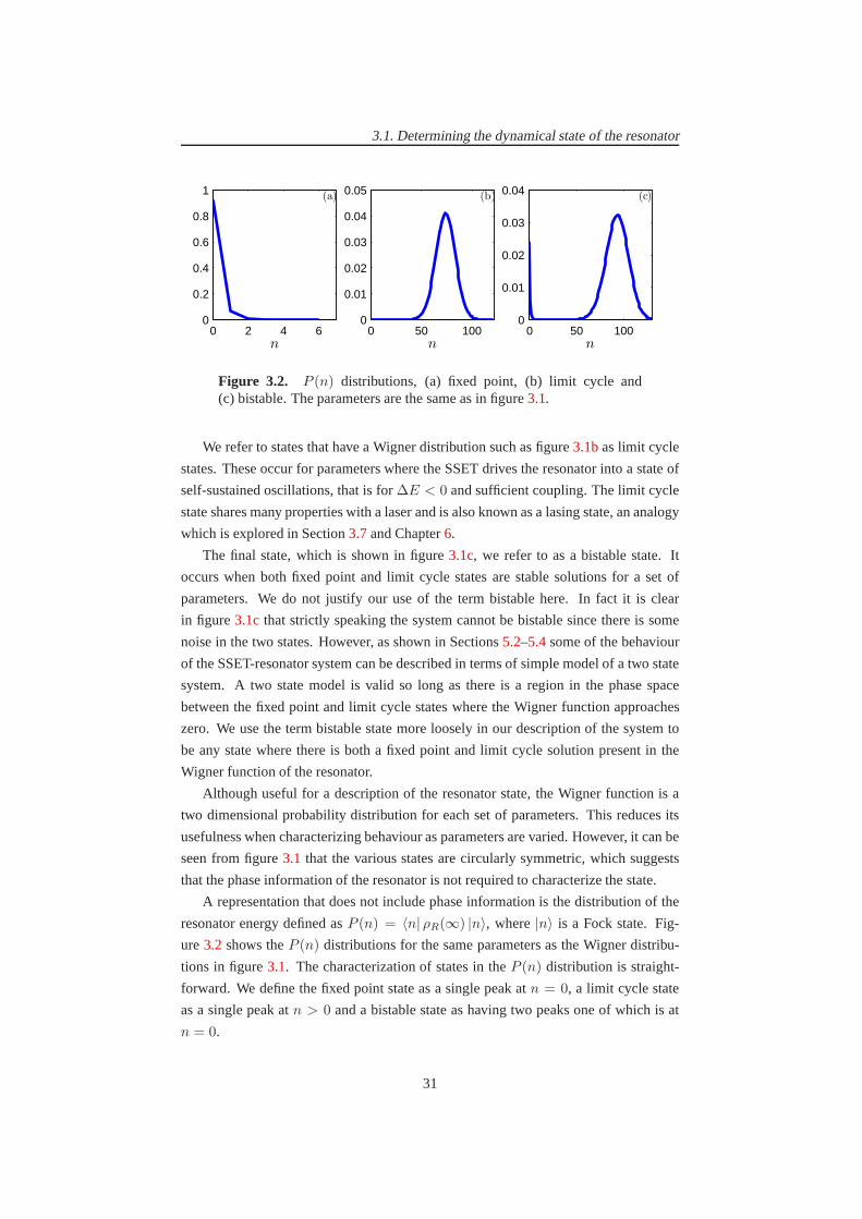
3.1. Determining the dynamical state of the resonator
0 2 4 60
0.2
0.4
0.6
0.8
1
n
(a)
0 50 1000
0.01
0.02
0.03
0.04
0.05
n
(b)
0 50 1000
0.01
0.02
0.03
0.04
n
(c)
Figure 3.2. P (n) distributions, (a) fixed point, (b) limit cycle and(c) bistable. The parameters are the same as in figure3.1.
We refer to states that have a Wigner distribution such as figure3.1bas limit cycle
states. These occur for parameters where the SSET drives theresonator into a state of
self-sustained oscillations, that is for∆E < 0 and sufficient coupling. The limit cycle
state shares many properties with a laser and is also known asa lasing state, an analogy
which is explored in Section3.7and Chapter6.
The final state, which is shown in figure3.1c, we refer to as a bistable state. It
occurs when both fixed point and limit cycle states are stablesolutions for a set of
parameters. We do not justify our use of the term bistable here. In fact it is clear
in figure3.1cthat strictly speaking the system cannot be bistable since there is some
noise in the two states. However, as shown in Sections5.2–5.4some of the behaviour
of the SSET-resonator system can be described in terms of simple model of a two state
system. A two state model is valid so long as there is a region in the phase space
between the fixed point and limit cycle states where the Wigner function approaches
zero. We use the term bistable state more loosely in our description of the system to
be any state where there is both a fixed point and limit cycle solution present in the
Wigner function of the resonator.
Although useful for a description of the resonator state, the Wigner function is a
two dimensional probability distribution for each set of parameters. This reduces its
usefulness when characterizing behaviour as parameters are varied. However, it can be
seen from figure3.1 that the various states are circularly symmetric, which suggests
that the phase information of the resonator is not required to characterize the state.
A representation that does not include phase information isthe distribution of the
resonator energy defined asP (n) = 〈n| ρR(∞) |n〉, where|n〉 is a Fock state. Fig-
ure3.2 shows theP (n) distributions for the same parameters as the Wigner distribu-
tions in figure3.1. The characterization of states in theP (n) distribution is straight-
forward. We define the fixed point state as a single peak atn = 0, a limit cycle state
as a single peak atn > 0 and a bistable state as having two peaks one of which is at
n = 0.
31

3.2. Current and current noise of a SSET
Plots can be made of theP (n) distribution as a parameter is varied (e.g. fig-
ure 3.21). However, as we show in Sections3.3–3.6 the state of the resonator can
be inferred quite effectively by looking at just the first twocumulants of theP (n)
distribution, which are the average energy,〈n〉 and the variance⟨
n2⟩
.
3.2 Current and current noise of a SSET
We start by reviewing the characteristics of the SSET in the uncoupled limit,κ → 0.
The current,〈I〉κ=0, and zero frequency Fano factor of the current noise,Fκ=0I (0), for
a SSET tuned to the JQP resonance are given by [17, 47],
〈I〉κ=0=
2eE2JΓ
4∆E2 + ~2Γ2 + 3E2J
, (3.2.1)
Fκ=0I (0) = 2 − 8E2
J
(
E2J + 2~
2Γ2)
(4∆E2 + ~2Γ2 + 3E2J )
2 , (3.2.2)
and are shown in figure3.3. The current has a peak at the centre of the resonance
∆E = 0, which has a width determined byΓ andEJ and was discussed previously in
Section2.2.2. Far from resonanceFκ=0I (0) has a value of 2. This is because for large
detuning the probability to be in the|2〉 state is always small (it is proportional to the
current). Due to the low current the charge is effectively transported in pairs, since the
time between the two quasi-particles in each JQP cycle will always be small. Due to
the large time between the breaking up of the Cooper pairs each pair is independent and
so follows Poissonian statistics. The transport is equivalent to a single tunnel junction
with a charge carrier of2e. This result is more general and in any transport process
that has Poissonian statistics the zero frequency current Fano factor can be used to find
the effective charge of the carrier, an example of which is the fractional quantum hall
effect [74–76].
Close to the centre of the resonance there is a strong interplay between the coherent
transfer of Cooper pairs and the quasi-particle tunnellingwhich results in a suppression
of the noise. The reason being that the probability of the|2〉 state no longer remains
small and so the time it takes for the system to evolve from the|0〉 state to the|2〉 state
is reflected in a more ordered transport process. This suppression is strongest at the
centre of the resonance where the coherent motion of Cooper pairs is most important.
3.3 Frequency regimes of operation
There is a large parameter space for the system that can be explored. We will not
attempt to investigate all of this here, but instead try to split the parameter space into
smaller regions that can be investigated more closely. As discussed in Section2.4we
32

3.3. Frequency regimes of operation
−0.2 0 0.20
0.05
0.1
0.15
0.2
0.25
∆E/eVds
〈I〉/
eΓ
(a)
−0.2 0 0.2
0.8
1
1.2
1.4
1.6
1.8
2
∆E/eVdsF
I(0
)
(b)
Figure 3.3. current (a) and current noise (b) of a SSET tuned to the JQPresonance. The parameters used areEJ = 1/16 eVds andr = 1.
user = 1 andEJ = 1/16 eVds throughout. We give the time-scales of the system in
terms ofΓ, which we can think of as the typical time-scale of the SSET sinceEJ . ~Γ.
For the resonator parameters we must choose the external damping, γext, to be
somewhat larger than what would be expected in experiment inorder to ensure the
resonator can be described by a limited number of energy states. For the frequency of
the resonator we identify three regimes in comparison to thetime-scale of the SSET.
These are whereΩ ≫ Γ, whereΩ ≪ Γ and whereΩ ≃ Γ. In this section we look at
how they are connected before we discuss each of them in detail in Sections3.4, 3.5
and3.6.
In Section3.1 it was shown how theP (n) distribution can be used to characterize
the state of the resonator. To explore a wide range of parameters it is easier to work
with a few cumulants of theP (n) distribution. The full set of cumulants contains the
same information as theP (n) distribution, but we do not necessarily need them all to
gain a lot of information about the system. In fact the first two, the average energy〈n〉and the variance
⟨
n2⟩
=⟨
n2⟩
− 〈n〉2, wheren is the number operator,n ≡ a†a, are
sufficient for our purposes. Rather than the variance we plotthe resonator Fano factor
Fn =⟨
n2⟩
/ 〈n〉. Just like the current Fano factor the Fano factor here is an indication
of the relationship of the distribution to a Poissonian distribution. A sub-Poissonian
resonator Fano factor indicates number squeezing of the resonator distribution, which
is a non-classical state [48, 73, 77].
We will look at these moments as a function of the detuning,∆E, and the resonator
frequency in relation to the SSET time-scale,Ω/Γ. Figure3.4provides an overview of
how the resonator behaves in terms of the average occupationnumber〈n〉. The average
33

3.3. Frequency regimes of operation
−1.5 −1 −0.5 0 0.5
0.5
1
1.5
2
2.5
3
3.5
4
4.5
5
∆E/eVds
Ω/Γ
0.00021
0.0029
0.039
0.52
7
94
Figure 3.4. Average energy,〈n〉, of the resonator as a function of thedetuning from resonance and resonator frequency forκ = 0.005, EJ =1/16 eVds, γext = 8 × 10⁻⁴ Γ, r = 1 and next = 0. Colours are on alog10 scale.
energy of the resonator is~Ω 〈n〉, so we also refer to〈n〉 as the average energy. For
negative detuning large values of〈n〉 are seen, which correspond to the driving of the
resonator into limit cycle states. From the average energy it is not clear where the
transitions occur or how they occur. Generally we see two kinds of transition. The
most common is a continuous transition, where the system evolves smoothly between
dynamical states. The second is a discontinuous transitionwhere the system changes
state via a bistability and we see a rapid change in the state.
The location of the transitions and what type they are is indicated quite faithfully
by the resonator Fano factor,Fn, as shown in figure3.5. It can be seen that this has
a peak around the region of large〈n〉. The peak to the left of the central limit cycle
region is rather large compared to the peak on the right of theregion. This large peak
corresponds to the bistable region and elsewhere we have a continuous transition. Other
features of the plot will be explained in the following sections. The location and nature
of the transition can be confirmed by use of theP (n) distribution.
We can compare the resonator moments with the current and current noise for the
same parameters as shown in figures3.6 and3.7. Broadly speaking〈I〉 shares many
similar features with〈n〉 andFI(0) with Fn. We will discuss further the extent to
which this is true by looking at the three frequency regimes in more detail.
34

3.3. Frequency regimes of operation
−1.5 −1 −0.5 0 0.5
0.5
1
1.5
2
2.5
3
3.5
4
4.5
5
∆E/eVds
Ω/Γ
0.73
1.9
5.1
14
36
94
Figure 3.5.Resonator Fano factor,Fn, as a function of the detuning fromresonance and resonator frequency for the same parameters as figure3.4.Colours are on alog10 scale.
−1.5 −1 −0.5 0 0.5
0.5
1
1.5
2
2.5
3
3.5
4
4.5
5
∆E/eVds
Ω/Γ
0.00022
0.00085
0.0034
0.013
0.052
0.21
Figure 3.6.Average SSET current,〈I〉, as a function of the detuning fromresonance and resonator frequency for the same parameters as figure3.4.Colours are on alog10 scale.
35

3.4. High frequency resonatorΩ ≫ Γ
−1.5 −1 −0.5 0 0.5
0.5
1
1.5
2
2.5
3
3.5
4
4.5
5
∆E/eVds
Ω/Γ
0.99
21
430
9100
190000
4000000
Figure 3.7. Current noise,FI(0), as a function of the detuning from res-onance and resonator frequency for the same parameters as figure 3.4.Colours are on alog10 scale.
3.4 High frequency resonatorΩ ≫ Γ
In the high frequency regime discrete peaks are seen in〈n〉 for ∆E < 0, as shown
in figure 3.4. These correspond to resonant absorption of energy by the resonator.
Less clear are the dips in〈n〉 that are observed for∆E > 0, which correspond to the
resonant emission of energy by the resonator i.e. the resonator can be cooled here if the
external temperature is large [18, 19]. For the weak coupling values that we consider
here, the resonances can be located by the matching of the resonator frequency to a
multiple of the eigenenergy of the SSET.
k~Ω = ±√
∆E2 + E2J , (3.4.1)
wherek is a non-zero integer and the sign on the right hand side should be the same as
the sign of∆E, so that resonances fork < 0 correspond to driving of the resonator.
For largeΩ we will have∆E ≫ EJ at these resonances and so their location is almost
entirely determined by∆E.
To see in more detail the effect of this resonance on the resonator state, figure3.8
shows〈n〉, Fn, 〈I〉 andFI(0) around thek = −1 resonance as∆E and the coupling,
κ, are varied. From figure3.8it can be seen that as the coupling is increased the system
undergoes a transition, which is from a fixed point to a limit cycle state. The limit cycle
region grows for larger couplings to occur further from the exact resonance condition.
36

3.4. High frequency resonatorΩ ≫ Γ
The value of〈n〉 indicates the size of the limit cycle, which grows with the coupling
strength and is largest on resonance. However, the value of〈n〉 only gives an indication
of where a transition occurs as it increases steadily through the transition.
Fn is better indicator of the position of the transition as it isstrongly peaked at the
transition. To move from a fixed point state to a limit cycle state involves a transition
through a state with a large variance. This transition can occur in two ways. The first
is a bistable transition where there are two peaks in theP (n) distribution. A bistable
state must have a high variance since〈n〉 will be somewhere in between the peaks. The
second type of transition is a continuous transition where the fixed point state smoothly
evolves to a limit cycle state with a small amplitude which then grows progressively as
we move further into the limit cycle region. During the transition we will go through
states which have the bell shape of figure3.2b but at small amplitude so that there
will be a sharp cut-off in the distribution atn = 0, an example of which is shown in
figure3.9. This type of state will also have a large variance although smaller than the
bistability.
In the limit cycleFn can become very low even becoming sub-Poissonian by drop-
ping below 1 suggesting a non-classical state. The current noise is very similar toFn
and can also become sub-Poissonian. However, there is no direct correlation between
Fn < 1 andFI(0) < 1 they may occur at the same time or separately [24]. A sim-
ilar result was obtained in [78] for a SET coupled to a resonator. They found that by
changing the bias voltage and the asymmetry of the junctionsany combination of sub-
and super-Poissonian values ofFn andFI(0) could be obtained.
The plot of〈I〉 takes a very similar form to that for〈n〉. Indeed a plot of〈I〉 / 〈n〉shows that, to a good approximation, there is a constant multiplier relating the two
within the limit cycle region as shown by figure3.10. The factor can be found by a
simple argument due to energy conservation. In order for a Cooper pair to move from
the lead to the island it must dissipate an amount of energy√
∆E2 + E2J ≃ |∆E|.
Without the coupling to the resonator the current at this large detuning is negligibly
small. We can therefore assume that the energy is entirely absorbed by the resonator.
The rate of energy gain by the resonator is therefore,〈I〉2e |∆E|. In the steady-state this
must be balanced by the energy loss of the resonator due to damping by the environ-
ment, which occurs at a rateγext~Ω 〈n〉. We therefore expect the relationship,
〈I〉 =~Ω
|∆E|2eγext 〈n〉 ≃2eγext
|k| 〈n〉 , (3.4.2)
where we have used the resonance condition given by equation3.4.1. It can be seen in
figure3.10that this is indeed the case.
A peak in〈n〉 is also seen in figure3.4at ∆E = 0, but this has a different origin.
It is due to heating of the resonator by the charge noise on theSSET island and there is
no dynamical transition in the state of the resonator. The peak corresponds to the JQP
37

3.4. High frequency resonatorΩ ≫ Γ
10
15
20
25
30
∆E/eVds
κ
10
15
20
25
30
∆E/eVds
κ
-1.7 -1.7-1.47 -1.47
0.26 1.3140 9.4〈n〉 Fn
×10−4 ×10⁻⁴
10
15
20
25
30
∆E/eVds
κ
10
15
20
25
30
∆E/eVds
κ
-1.7 -1.7-1.47 -1.47
0.00083 2.20.081 330〈I〉 FI
×10−4 ×10⁻⁴
Figure 3.8. 〈n〉, Fn, 〈I〉 andFI(0) as a function of the detuning fromresonance and coupling strength forΩ = 10 Γ, EJ = 1/16 eVds, γext =3×10⁻⁴ Γ, r = 1 andnext = 0. The dashed line indicates the transition indynamical state from fixed point to limit cycle via a continuous transitionas the coupling is increased.
38

3.4. High frequency resonatorΩ ≫ Γ
0 50 100 1500
0.005
0.01
0.015
0.02
0.025
n
P(n
)
Figure 3.9. P (n) distribution for a continuous transition for∆E =−1.59 andκ = 1.3 × 10⁻³, with the other parameters the same as fig-ure3.8.
−1.7 −1.65 −1.6 −1.55 −1.51
1.2
1.4
1.6
1.8
2
2.2
2.4
2.6
2.8
3x 10
−3
∆E/eVds
κ
0.98
2
3.1
4.1
5.2
6.3
Figure 3.10. 〈I〉 /2eΓ 〈n〉 γext as a function of the detuning from reso-nance and coupling strength. The parameters are the same as figure3.8.The dashed line indicates the transition from fixed point to limit cyclestate as the coupling is increased.
39

3.5. Low frequency resonatorΩ ≪ Γ
peak seen in the current in figure3.6. We will discuss in Chapter4 how the SSET acts
as an effective thermal bath for the resonator in the low frequency and low coupling
regime.
3.5 Low frequency resonatorΩ ≪ Γ
The resonances described by equation3.4.1will have a width related to the coupling,
κ, and quasi-particle tunnelling rate,Γ. In the regimeΩ ≪ Γ the resonances will
no longer be distinguishable. Also note that as the frequency is reduced some of the
resonances become disallowed. This occurs whenk~Ω < EJ but will not be observed
here sinceEJ < ~Γ.
Transfer of energy between the SSET and resonator still occurs in this regime with
the direction given by the sign of∆E but is now non-resonant [20]. Figure3.11shows
the average energy,〈n〉, as the detuning and coupling are varied. The transitions be-
tween the three different dynamical states of the resonatorare indicated by dashed
lines in the figure. For∆E < 0 energy is transferred to the resonator and for strong
enough coupling the resonator is driven into the limit cyclestate which grows in size
as∆E becomes more negative. Forκ & 0.0011 when∆E is sufficiently negative
(∆E ≃ −0.15 eVds) the resonator enters the bistable regime and then undergoes a
transition back to the fixed point state in which the limit cycle disappears abruptly [23].
Unlike the high frequency case there is not a strong correspondence between〈n〉and〈I〉 as can be seen by comparing figures3.11and3.12. In fact the current is always
dominated by the JQP current peak of the SSET. There is some modification, however,
which can be seen more clearly by subtracting off the background (uncoupled) current
as given by equation3.2.1, which is what we do in Chapter4.
As in the high frequency case,Fn is peaked around the transitions between the fixed
point and limit cycle states, figure3.13. The strongest feature occurs in the vicinity of
the bistable region. The peak at the continuous transition is not as clear as theΩ ≫ Γ
case.
Fn can be compared with the zero frequency current noise shown in figure3.14as
before. For weak coupling a dip can be seen inFI(0) along the∆E = 0 line, which is
due to the suppression of the current noise present in the uncoupled case (figure3.3).
For stronger coupling, peaks are seen at the transitions as seen in theFn plot. However,
the correspondence betweenFI(0) andFn is not as strong as for the high frequency
case. In particular we see a minimum inFI(0) to the right of the bistable region that
extends down to zero coupling. This feature will be explained in Section4.5, but here it
demonstrates that the zero frequency noise contains more information about the system
than just measuring average properties or moments.
40

3.5. Low frequency resonatorΩ ≪ Γ
−0.3 −0.2 −0.1 0 0.1 0.2 0.3
0.2
0.4
0.6
0.8
1
1.2
1.4
1.6
1.8
2x 10
−3
∆E/eVds
κ
1.8
20
37
55
73
91
Figure 3.11.Average energy of the resonator as a function of the detuningfrom resonance and coupling strength forΩ = 0.12 Γ, EJ = 1/16 eVds,γext = 1 × 10⁻⁴ Γ, r = 1 and next = 2. The dashed lines indicatetransitions between dynamical states: for most of the rangeconsideredthe resonator is in the fixed point state, but for large enoughcoupling atransition to the limit cycle state occurs close to the centre of the reso-nance. The bistable region is the smallest and occurs forκ > 0.0011 and∆E ≃ −0.15 eVds.
−0.3 −0.2 −0.1 0 0.1 0.2 0.3
0.2
0.4
0.6
0.8
1
1.2
1.4
1.6
1.8
2x 10
−3
∆E/eVds
κ
0.02
0.058
0.096
0.13
0.17
0.21
Figure 3.12.Current through the SSET as a function of the detuning fromresonance and coupling strength. The dashed lines indicatetransitions inthe resonator’s state and the parameters are the same as in figure3.11.
41

3.5. Low frequency resonatorΩ ≪ Γ
−0.3 −0.2 −0.1 0 0.1 0.2 0.3
0.2
0.4
0.6
0.8
1
1.2
1.4
1.6
1.8
2x 10
−3
∆E/eVds
κ
2.9
5.1
9.1
16
29
51
Figure 3.13.Resonator Fano factor,Fn as a function of the detuning fromresonance and coupling strength. The dashed lines indicatetransitions inthe resonator’s state and the parameters are the same as in figure3.11andthe colours are on alog10 scale.
−0.3 −0.2 −0.1 0 0.1 0.2 0.3
0.2
0.4
0.6
0.8
1
1.2
1.4
1.6
1.8
2x 10
−3
∆E/eVds
κ
0.76
3
12
48
190
770
Figure 3.14. Current noise,FI(0), as a function of the detuning fromresonance and coupling strength. The dashed lines indicatetransitions inthe resonator’s state and the parameters are the same as in figure3.11andthe colours are on alog10 scale.
42

3.6. Strongly interacting regimeΩ ∼ Γ
−1 −0.5 0 0.5
1
2
3
4
5
6
7
8x 10
−3
∆E/eVds
κ
0.00021
17
34
52
69
86
Figure 3.15.Average energy of the resonator as a function of the detuningfrom resonance and coupling strength forΩ = 2 Γ, EJ = 1/16 eVds,γext = 8 × 10⁻⁴ Γ, r = 1 andnext = 0.
3.6 Strongly interacting regimeΩ ∼ Γ
The final operating regime we consider for the device is whereΩ ∼ Γ. At this point
the matching of the electrical and mechanical time-scales leads to a relatively strong
mutual interaction.
Figure3.15show the average energy of the resonator as the detuning and coupling
are varied. The resonances corresponding to the absorptionof one or two photons
(k = −1 andk = −2 in equation3.4.1) can clearly be seen in the figure. Thek = −2
resonance requires a stronger coupling than thek = −1 resonance to be allowed since
it is a higher order process. Figure3.16shows the current for the same parameters.
Peaks are seen in the current due to the same resonances as in〈n〉. An additional peak
is seen due to the JQP peak of the SSET. The JQP current peak canbe seen to be
modified more strongly as the coupling is increased. The current for thek = −1 and
k = −2 resonances can be seen to be approximately equal. In contrast the average
energy of the resonator is larger for thek = −2 resonance. This can be understood
qualitatively from equation3.4.1. The equation states that if the current is the same at
thek = −1 andk = −2 resonances then the average energy should be twice as big for
thek = −2 resonance, which is seen to be the case. However, it is not understood why
the two currents are the same.
Figures3.17and3.18showFn andFI(0) respectively. A strong enhancement is
seen in both these quantities around the resonant peaks. Forthe k = −1 peak this
43

3.7. Analogy with a micromaser
−1 −0.5 0 0.5
1
2
3
4
5
6
7
8x 10
−3
∆E/eVds
κ
0.0019
0.044
0.085
0.13
0.17
0.21
Figure 3.16. Current as a function of the detuning from resonance andcoupling strength for the same parameters as figure3.15.
corresponds to a continuous transition from fixed point to limit cycle state. For the
k = −2 peak the noise is much larger at the transition and corresponds to a bistable
transition. Evidence of thek = −3 resonance is also seen in the noise although the
coupling is not sufficiently strong to observe a feature in〈n〉 or 〈I〉. The plots ofFn
andFI(0) are generally in agreement with two notable exceptions. For∆E ≃ −0.2
andκ ≃ 2 × 10⁻³ a peak is seen inFn that is not present inFI(0). A similar feature
was also observed in the low frequency case and will be explained in Section4.5.
Also within thek = −1 resonanceFn can be seen to reduce on resonance to a sub-
Poissonian value. However, a peak is seen inFI(0) on the resonance. We will return
to this feature in Section6.3.
3.7 Analogy with a micromaser
The instabilities seen in this system are similar to those seen in quantum optical sys-
tems. In particular we find close analogies with the micromaser system [22, 23]. The
micromaser [79] consists of a superconducting cavity resonator through which a beam
of two level atoms prepared in the excited state is sent. The beam is of low intensity
so that only one atom is in the cavity at any one time. While in the cavity the atoms
can exchange energy with the resonator and so excite or cool it when on resonance.
This is analogous to the SSET resonator system where the Cooper pairs are transported
through the system one at a time and so play the role of the atoms.
44

3.7. Analogy with a micromaser
−1 −0.5 0 0.5
1
2
3
4
5
6
7
8x 10
−3
∆E/eVds
κ
0.78
1.9
4.8
12
30
74
Figure 3.17. Resonator Fano factor,Fn as a function of the detuningfrom resonance and coupling strength. The parameters are the same as infigure3.15and the colours are on alog10 scale.
−1 −0.5 0 0.5
1
2
3
4
5
6
7
8x 10
−3
∆E/eVds
κ
0.76
9.1
110
1300
15000
190000
Figure 3.18. Current Fano factor,FI(0), as a function of the detuningfrom resonance and coupling strength. The parameters are the same as infigure3.15and the colours are on alog10 scale.
45

3.7. Analogy with a micromaser
There is, however, an important difference between the two systems. In the mi-
cromaser the rate at which the atoms travel through the cavity is controlled externally
and so is not influenced by the interaction with the resonator. In our solid state sys-
tem, however, the back-action of the resonator on the SSET modifies the current. This
makes the system more complex, but also allows us to use the current as a probe of the
behaviour of the system, which cannot be done in the micromaser.
A series of dynamical transitions in the resonator state occur in the micromaser as
the coupling between the atoms and cavity is increased as shown in [79]. The transi-
tions are accompanied by jumps in the average energy of the resonator that correspond
to the formation of new stable limit cycle states. There is also an accompanying peak
in the variance of the resonator energy at the transition [79]. The transitions become
sharper as the number of atoms to pass through the cavity during the cavity lifetime is
increased. The transitions also become less sharp at highercoupling strengths.
We can carry out a similar analysis for the SSET-resonator system. The equivalent
of the rate of atoms through the cavity is the current and the lifetime of the cavity mode
is given by the external damping. Unlike the micromaser we cannot easily increase
the current without modifying the interaction between the SSET and resonator. It is
therefore easier to alter the external damping of the resonator, although this will also
cause a shift in the position of the transitions. We are also limited by the finite number
of resonator states and so cannot reach the limit where the transitions become sharp.
In figure3.19the normalized average energy is shown as the coupling is varied for
three values of the external damping. As the coupling is increased the resonator first
goes through a transition from fixed point to limit cycle state to reach a maximum value.
Further increasing the coupling causes the average energy to reduce until an increase
is seen corresponding to the formation of a second limit cycle state. The increase in
the average energy becomes sharper as the damping is reduced. The behaviour is also
observed in the variance of the energy as shown in figure3.20. The first peak is at
the transition from fixed point to limit cycle state. The second peak becomes much
more pronounced as the external damping is reduced. Also note that in-between the
two peaksFn < 1 indicating a sub-Poissonian distribution in the resonatorenergy as
previously observed [23].
The nature of the transitions is made clearer by observing the change in theP (n)
distribution as the coupling is varied. This is shown for thesmallest and largest values
of γext from figure3.19, in figures3.21and3.22respectively. It can be seen in the
figures that as the coupling is increased more stable limit cycle states of the system are
formed. For smallγext, as in figure3.21, it can be seen that the first limit cycle state
vanishes soon after the second is formed. It is for this reason that the jump in〈n〉 is
seen. For the larger value ofγext, shown in figure3.22, and for the further transitions
in figure3.21, it can be seen that the limit cycle states co-exist and so a sharp jump in
〈n〉 is not seen.
46

3.7. Analogy with a micromaser
0 0.05 0.1 0.15 0.2 0.250
0.1
0.2
0.3
0.4
0.5
0.6
0.7
0.8
0.9
1
√κ
〈n〉/
max(〈n
〉)
3 × 10⁻⁴
5 × 10⁻⁴
10 × 10−4
Figure 3.19.Normalized average energy of the resonator as a function ofthe coupling for 3 values of the external damping. The other parametersare∆E = −0.1 eVds, Ω = Γ, EJ = 1/16 eVds, r = 1 andnext = 0. Atransition is seen for
√κ ≃ 0.12 that becomes sharper for reducedγext
0 0.05 0.1 0.15 0.2 0.250
2
4
6
8
10
12
√κ
Fn
3 × 10⁻⁴
5 × 10⁻⁴
10 × 10−4
Figure 3.20.Fn as a function of the coupling for 3 values of the externaldamping. The parameters are the same as figure3.19. A transition is seenfor
√κ ≃ 0.12 that becomes sharper for reducedγext
47

3.7. Analogy with a micromaser
0.05 0.1 0.15 0.2 0.250
20
40
60
80
100
120
140
√κ
n
0
0.04
0.08
0.12
0.16
0.2
Figure 3.21.ChangingP (n) distribution as a function of the coupling forγext = 3×10⁻⁴ Γ. The other parameters are given in figure3.19. Dashedlines indicate the locations of peaks in the distribution.
0.05 0.1 0.15 0.2 0.250
10
20
30
40
50
60
√κ
n
0
0.05
0.1
0.15
0.2
0.25
Figure 3.22.ChangingP (n) distribution as a function of the coupling forγext = 0.001 Γ. The other parameters are given in figure3.19. Dashedlines indicate the locations of peaks in the distribution.
48

3.7. Analogy with a micromaser
The origin of the co-existing limit cycle states was explained in terms of the semi-
classical dynamics of the system in [22]. The driving of the resonator by the SSET
can be described by an effective damping rate. A stable limitcycle solution occurs
when this effective damping matches the external damping bythe resonator bath. The
effective damping is an oscillating function with the amplitude of the resonator and so
a number of solutions can co-exist.
49

Chapter 4
Resonator in a Thermal State
In the previous chapter we gave an overview of the behaviour of the system for a range
of parameters. In this chapter we remain in the regime of weakcoupling between the
SSET and resonator so that the resonator remains in the fixed point state throughout. In
this regime the SSET acts as an effective thermal bath for theresonator as described in
Section4.1. We focus on just one of the frequency regimes introduced in the previous
chapter, that ofΩ ≪ Γ, where the effective bath parameters have a simple analyti-
cal form. When this is the case the current and current noise can be described using
much simpler models than the solution of the full master equation. The first of these,
which is described in Section4.2, calculates the current and current noise by assuming
that the gate voltage fluctuates with statistics given by thethermal bath model of Sec-
tion 4.1. This simple model accurately describes the current, but not the current noise.
A full description of the system in this regime can be obtained from a set of mean field
equations as shown in Section4.3. The mean field equations for this system do not
form a closed set, but they can be truncated with little errorin the thermal regime by
making sensible approximations. The final model, describedin Section4.4, attempts
to capture the part of the current noise due to the dynamics ofthe resonator. Finally, in
Section4.5, the finite frequency current noise in this regime is calculated and to what
extent its behaviour is captured by the simple models is discussed.
4.1 SSET as an effective thermal bath
For sufficiently weak coupling, the steady-state of the resonator can be described an-
alytically. Based on the Born-Markov master equation that was described in Sec-
tion 2.4the SSET degrees of freedom can be traced over and the state ofthe resonator
found [18]. Alternatively general linear response methods [80] can be applied to the
system to describe the resonator [19].
The result from these two approaches is that for weak coupling and small mechan-
50
4.1. SSET as an effective thermal bath
ical displacement the SSET acts on the resonator as an effective thermal bath. The
thermal bath is characterized by three parameters, an effective damping,γSSET, an ef-
fective occupation number,nSSET, and a renormalization of the resonator frequency
to ΩR. Using either the Born-Markov or linear response methods the values of these
parameters in the regimeΩ ≪ Γ are [18, 19],
γSSET =16mx2
sΩ4E2
J∆E
Γ
[
4∆E2 + 13~2Γ2 + 10E2
J
(4∆E2 + ~2Γ2 + 3E2J)
3
]
, (4.1.1)
nSSET =~
2Γ2 + 4∆E2
16∆E~Ω, (4.1.2)
Ω2R = Ω2
(
1 − 48mΩ2xsE2J∆E
(4∆E2 + ~2Γ2 + 3E2J)
2
)
. (4.1.3)
We focus on theΩ ≪ Γ regime here where the parameters have the simple form
above. However, the effective thermal bath description canbe extended to all frequency
regimes, so long as the coupling is weak [81].
In the same manner as a resonator coupled to a standard thermal bath, the steady-
state of the resonator will have the form of a thermal state (i.e. the Wigner function will
take a Gaussian form). In practice there is also the thermal bath due to the resonators
surroundings and the average occupation number of the resonator,n, is found from a
weighted average of the two baths [57],
n =γextnext + γSSETnSSET
γext + γSSET. (4.1.4)
The total damping rate of the resonator,γ, is given by a sum of the damping due to the
SSET and the external damping due to the resonators surroundings,
γ = γext + γSSET (4.1.5)
In figure4.1 the shape ofγSSET andnSSET are shown as a function of the detuning.
γSSET is negative for∆E < 0 and so in this region the total damping of the resonator
is reduced. For sufficiently strong coupling the total damping can become negative and
this weak coupling description clearly breaks down since the fluctuations in the position
of the resonator are no longer small. To ensure that the modelaccurately describes the
state of the resonator we require thatγext > |γSSET|. nSSET is also negative for
∆E < 0 so the productγSSETnSSET appearing in equation4.1.4is always positive.
When∆E < 0 the coupling with the SSET must increase the value ofn abovenext.
However, for∆E > 0, n can be reduced due to the coupling with the SSET and so the
resonator can be cooled [18, 19, 21].
The coupling to the SSET also leads to a shift in the average position of the res-
onator which has a simple relationship to the average chargeon the SSET island,
51

4.1. SSET as an effective thermal bath
−0.2 0 0.2−3
−2
−1
0
1
2
3x 10
−6
∆E/eVds
γSSE
T(a)
−0.2 0 0.2−100
−50
0
50
100
∆E/eVds
nSSE
T
(b)
Figure 4.1. (a)γSSET (b) nSSET as a function of∆E as calculated fromequations4.1.1and4.1.2. Parameters areκ = 1 × 10⁻⁴, Ω = 0.05 Γ,EJ = 1/16 eVds, γext = 1 × 10⁻⁴ Γ andnext = 2
which is in turn proportional to the average (steady-state)current flowing through the
SSET [18, 22]. The average displacement is given by,
〈x〉 = − 3xs
2eΓ〈I〉 . (4.1.6)
In Section4.3we derive this relationship using the mean field equations.
For weak SSET-resonator coupling the changes in the transport properties of the
SSET due to the resonator are relatively small so it makes sense to examine just the
difference between the values for the coupled and uncoupledcases. The uncoupled
current,〈I〉κ=0, and zero frequency current Fano factor,Fκ=0I (0), were given in equa-
tions3.2.1and3.2.2respectively.
The change in the SSET current due to the coupling with the resonator (calculated
numerically) is shown in figure4.2. We consider a slow resonatorΩ ≪ Γ and very
weak coupling so that although the SSET has quite a strong influence on the resonator
state, the resonator nevertheless remains in a thermal state which is well described by
equations4.1.1–4.1.5. From figure4.2we see that near the centre of the resonance the
current is suppressed by the resonator, but on either side ofthis there is an enhancement.
The current noise is modified in a similar way to the current, but in the opposite sense,
as shown in figure4.3, thus there is an increase in the noise near to the resonance with
a decrease on either side.
Although it is relatively easy to calculate the current and current noise numerically
it is helpful to develop simple analytical models of the coupled system so that the
results can be better understood. The starting point for these models is that a thermal
52

4.1. SSET as an effective thermal bath
−0.3 −0.2 −0.1 0 0.1 0.2 0.3−2.5
−2
−1.5
−1
−0.5
0
0.5
1x 10
−4
∆E/eVds
(
〈I〉−
〈I〉κ
=0)
/eΓ
numfl
Figure 4.2.Change in current through the SSET as a function of∆E. Thecurves are labelled asnumfor the numerical results andfl for the changein the current calculated using equation4.2.3. The parameters used are thesame as in figure4.1. [Note that for these parametersn varies from a valueof 2 far from resonance to a peak value of 2.28 at∆E = −0.01 eVds.γSSET/γext has maxima and minima of±0.029 at∆E = ±0.044 eVds.]
−0.3 −0.2 −0.1 0 0.1 0.2 0.3−3
−2
−1
0
1
2
3
4
5
6x 10
−3
∆E/eVds
FI(0
)−
Fκ=
0
I(0
)
numflmean2mean3
Figure 4.3.Change in the zero frequency current Fano factor of the SSETdue to the resonator. The curves are labelled asnum for the numericalresults,fl is obtained from equation4.2.6, mean2is calculated using thesecond order mean field equations andmean3using the third order meanfield equations. The parameters used are the same as in figure4.1.
53

4.2. Fluctuating gate model
state has a Gaussian distribution in position and momentum space [82]. A Gaussian
distribution is entirely described by second order moments, a fact which we can use to
our advantage.
4.2 Fluctuating gate model
The simplest way of including the influence of the resonator on the SSET is to include
the effect of fluctuations in the position of the resonator onthe current [24]. Because
the resonator acts as a gate for the SSET island, a shift of theposition of the resonator
leads to an effective change in the detuning energy∆E (equation2.4.3). Hence, when
the resonator position fluctuates so will the detuning energy. We can incorporate the
effect of the mechanical motion into the expression for the current, equation3.2.1, by
calculating it for a fixed position before averaging over theresonator state, an approach
that was also used in [83]. We make the replacement∆E → ∆E+2mΩ2xsx to obtain
the current,
I(x) =2eE2
JΓ
4 (∆E + 2mΩ2xsx)2 + ~2Γ2 + 3E2J
=2eE2
JΓ
β + α(x)(4.2.1)
where we have definedβ ≡ 4∆E + ~2Γ2 + 3E2
J andα(x) = 16mΩ2xs(∆Ex +
mΩ2xsx2). Assuming the shift term is small, we perform a Taylor expansion of the
current aboutα(0) = 0 to second order.
I(x) ≃ I(0) + α∂I(x)
∂α(x)
∣
∣
∣
∣
α(x)=0
+ α2 ∂2I(x)
∂α(x)2
∣
∣
∣
∣
α(x)=0
, (4.2.2)
and then take the average over the resonator position. Keeping terms up to orderx2s we
obtain,
〈I〉fl = I(0)
[
1 − 16mΩ2xs
β
∆E 〈x〉 + mΩ2xs
⟨
x2⟩
(
1 − 16∆E2
β
)]
= I(0)β2 − 16(mΩ2xs)
2⟨
x2⟩ (
β − 16∆E2)
β2 − 48mΩ2x2s∆EE2
J
, (4.2.3)
where the averages are taken over the (Gaussian) steady state probability distribution
of the resonator. In the second line we have used equation4.1.6to eliminate〈x〉. The
value of⟨
x2⟩
≃⟨
x2⟩
is calculated using equation4.1.4. Although we have eliminated
〈x〉 we can also approximate it to high accuracy using the uncoupled current in place
of the actual current in equation4.1.6.
It is clear from figure4.2 that equation4.2.3accurately describes the modification
54

4.2. Fluctuating gate model
to the current due to the presence of the resonator. Thus in this weak coupling regime
where the resonator remains in a thermal state, the modification of the current is simply
due to two affects. A shift in the resonator’s position givesan asymmetric shape. From
equation4.1.6this position shift will be negative so from equation4.2.3the current
will increase for∆E > 0 and decrease for∆E < 0. Secondly a smearing out of the
JQP current peak due to fluctuations in the resonator position will tend to reduce the
current near to the peak and increase it either side. We see from equation4.2.3that the
decrease will be when12∆E2 < ~2Γ2 + 3E2
J .
For the current noise we naively replace∆E → ∆E +2mΩ2xsx in equation3.2.2
to obtain,
SI(x) = 4eI(x) − 32e2E4JΓ(
E2J + 2~
2Γ2)
(
4 (∆E + 2mΩ2xsx)2+ ~2Γ2 + 3E2
J
)3
= 4eI(x) − 4e2E2JΓφ
(β + α(x))3 , (4.2.4)
whereφ ≡ 8E2J
(
E2J + 2~
2Γ2)
. As for the current this expression is expanded about
α(0) keeping terms up to second order inxs and then the resonator position averaged
over.
SflI,I(0) =4e 〈I〉fl
− 4e2E2JΓφ
β3
[
1 − 48mΩ2xs
β
∆E 〈x〉 − mΩ2xs
⟨
x2⟩
(
1 − 32∆E2
β
)
]
,
(4.2.5)
=4e 〈I〉fl
[
1 − 72mΩ2x2sE
2Jφ∆E
β4
]
− 4e2E2JΓφ
β5
[
β2 − 48(
mΩ2xs
)2 ⟨x2⟩ (
β − 32∆E2)
]
(4.2.6)
The modification to the current noise is similar to that of thecurrent in that there is
an asymmetry due to a shift in the position of the resonator and a smearing out due to
fluctuations in the resonator position. However, sinceFI(0) is a dip rather than a peak
the changes in the current noise are in the opposite sense.
In contrast to the current, it can be seen from figure4.3 that for the Fano factor,
equation4.2.6does not capture the behaviour correctly. Although the qualitative shape
is the same with a central peak with dips either side, the curves do not match and the
asymmetry of the numerical curve is in the opposite direction to that predicted by the
simple model.
The reason for the disagreement in the current noise is that the simple model of a
fluctuating gate neglects both the correlations between theelectrical and mechanical
55

4.3. Mean field equations
motion and the dynamics of the resonator. The current noise (in contrast to the average
current) is sensitive to the correlations between the SSET charge and the resonator
motion and hence to describe it accurately we need to includethem in some way.
4.3 Mean field equations
A straightforward and systematic way to include correlations and information about the
resonator dynamics are the mean field equations of the system, namely the equations
of motion for the expectation values of the SSET and resonator operators. The mean
field equations are generated in turn by multiplying the master equation by an operator
(or product of operators) and taking the trace over the full system [22].
For the SSET operators we have the five equations,
〈p0〉t = iEJ
2~
(
〈c〉t −⟨
c†⟩
t
)
+ Γ 〈p1〉t , (4.3.1)
〈p1〉t = −Γ 〈p1〉t + Γ 〈p2〉t , (4.3.2)
〈p2〉t = −iEJ
2~
(
〈c〉t −⟨
c†⟩
t
)
− Γ 〈p2〉t , (4.3.3)
〈c〉t =
(
−i∆E
~− Γ
2
)
〈c〉t + iEJ
2~
(
〈p0〉t − 〈p2〉t)
− i2mΩ2xs
~〈xc〉t , (4.3.4)
⟨
c†⟩
t=
(
i∆E
~− Γ
2
)
⟨
c†⟩
t− i
EJ
2~
(
〈p0〉t − 〈p2〉t)
+ i2mΩ2xs
~
⟨
xc†⟩
t, (4.3.5)
where〈O〉t = Tr [Oρ(t)]. The coupling to the resonator appears in the last two of these
equations. We can also write down equations of motion for theresonator operators,
given here up to second order,
〈x〉t = 〈v〉t , (4.3.6)
〈v〉t = −Ω2 〈x〉t − xsΩ2(
〈p1〉t + 2 〈p2〉t)
− γext 〈v〉t , (4.3.7)⟨
x2⟩
t= 〈xv〉t + 〈vx〉t , (4.3.8)
⟨
v2⟩
t= −Ω2
(
〈xv〉t + 〈vx〉t)
− 2xsΩ2 (〈vp1〉t + 2 〈vp2〉t)
− 2γext
⟨
v2⟩
t+
γext~Ω
m(1 + 2next) , (4.3.9)
〈xv〉t + 〈vx〉t = 2⟨
v2⟩
t− 2Ω2
⟨
x2⟩
t− 2xsΩ
2(
〈xp1〉t + 2 〈xp2〉t)
− γext
(
〈xv〉t + 〈vx〉t)
. (4.3.10)
From these equations we can derive some useful relationships and obtain equation4.1.6.
From a trace over the charge and right hand junction current operators in the steady-
56

4.3. Mean field equations
state (equations2.7.3and2.7.8) we find,
〈Q〉 = e (〈p1〉 + 2 〈p2〉) , (4.3.11)
〈I〉 = eΓ (〈p1〉 + 〈p2〉) . (4.3.12)
Equation4.3.2gives that〈p1〉 = 〈p2〉 in the steady-state so the current and charge are
related by,
〈Q〉 =3
2Γ〈I〉 . (4.3.13)
Then, from equations4.3.6and4.3.7, the relationship between the average position
and average charge in the steady-state is established,
〈x〉 = −xs
e〈Q〉 , (4.3.14)
which when combined with equation4.3.13, leads immediately to equation4.1.6.
No matter what order we go to the set of mean field equations forthe SSET-
resonator system never forms a closed set. The equation for〈c〉 (equation4.3.4) con-
tains the second order term〈xc〉. Calculating the the equation of motion for〈xc〉 then
introduces a term⟨
x2c⟩
(see equationC.0.4) and so forth.
One approach to form a closed set of equations is to perform the semi-classical
approximation from quantum optics. In this approximation correlations between the
SSET and resonator are neglected (atom and field in quantum optics). The replacement
〈xc〉 → 〈x〉〈c〉 would therefore be made. It is known as the semi-classical approxima-
tion since the set of equations now describe a quantum mechanical device coupled to a
classical harmonic oscillator. The semi-classical approximation was used to investigate
the SSET-resonator system in [22].
In making the semi-classical approximation we remove some of the noise in the
system [22, 84]. From the mean field equations it is clear that higher order moments
of the resonator such as⟨
x2⟩
will not be involved. It is essential to include⟨
x2⟩
since
we know from the fluctuating gate model, in the previous section, that it is required
to describe the current. The state of the resonator is Gaussian to a very good approxi-
mation in the thermal regime. Any third order cumulants of resonator operators must
therefore be zero. It therefore seems sensible to extend theapproximation to include
the correlations of pairs of operators. In analogy to the semi-classical approximation,
in which it is assumed that second order cumulants of the system operators are zero,
we instead assume that third order cumulants are zero. The resulting replacements are
of the kind,⟨
x2c⟩
t→ 2 〈x〉t〈xc〉t +
(
⟨
x2⟩
t− 2 〈x〉2t
)
〈c〉t . (4.3.15)
Crucially the correlations between products of two operators are retained. Further de-
tails of the method and the resulting second order mean field equations are given in
57

4.3. Mean field equations
−0.3 −0.2 −0.1 0 0.1 0.2 0.35
5.1
5.2
5.3
5.4
5.5
5.6
∆E/eVds
〈x2〉
numappmean
Figure 4.4.Value of⟨
x2⟩
in the steady-state as given by the full numericalsolution (num), solving the second order non-linear mean field equations(mean) and from the analytical expression in equation4.1.4(app). Theparameters used are the same as in figure4.1.
AppendixC.
The resulting set of equations is closed, but is non-linear because of the terms gener-
ated by the approximation. The steady-state of the system can be found by numerically
solving the set of equations. In figure4.4 it is shown that the state of the resonator
as given by the value of⟨
x2⟩
is the same for the mean field equations as the full nu-
merical solution. Also shown in figure4.4 is the predicted value from equation4.1.4
(⟨
x2⟩
= x2zp (1 + 2n) for a thermal state), which also shows good agreement. The
value of the current in the steady-state obtained from the mean field equations is indis-
tinguishable from the results of the full numerical solution and fluctuating gate models,
shown in figure4.2, so is not shown here.
Although the set of non-linear equations fully describe theevolution of the system
the calculation of the current noise can be simplified by forming a set of linear equa-
tions. With a linear set of equations we can use a method equivalent to that described
in Section2.6 to find the noise spectrum. We can also calculate the eigenvalues of the
evolution, which we make use of below.
The non-linearity in the equations comes from the use of the cumulants to break
correlations in the system. Without breaking these correlations the evolution of the
SSET variables does not depend on equations for resonator operators alone. This sug-
gests that the equations of motion for the resonator variables alone are not required to
capture the resonator dynamics. The evolution of the resonator is included in the equa-
58

4.3. Mean field equations
tions of the form〈xc〉. To recover a set of linear equations we replace the expectation
values of resonator operators alone by their steady-state values. The steady-state values
can be determined either from the non-linear set of equations, the numerical results or
the thermal bath model described in Section4.1.
The new set of linear equations retains the correlations between the SSET operators
and position of the resonator and the dynamics of the resonator position. However, the
set of second order non-linear equations also contained thedynamics of⟨
x2⟩
t. To
include the same dynamics in the linearized equations we therefore have to extend the
equations to third order, so that the dynamics of⟨
x2⟩
tare included in terms such as
⟨
˙x2c⟩
t. We then apply the approximation to products of four operators. Note that
this extension to higher order is only to include the correctdynamics of the resonator
it is not because the resonator state is not Gaussian (we still use only second order
moments to describe the resonator state). The third order set of linearized equations
includes both the dynamics and correlations that are present in the set of second order
non-linear equations.
The linearized equations can be written in the form,
p(t) = Ap(t), (4.3.16)
wherep(t) is a vector of the moments of the system andA is a matrix that describes
the evolution. The moments should be in a dimensionless formso thatA then has
dimensions oftime−1. The form of this equation is similar to equation2.4.1with A
analogous to the Liouvillian,L. Both equations describe the evolution of the same
system but equation4.3.16describes the evolution of a number of mean quantities and
is approximate. The steady-state of the linear equations isgiven by the null right hand
eigenvector ofA, r0, and should of course have the same result as the second order
non-linear equations.
The calculation of the charge noise spectrum and current noise spectrum for the
left hand junction can be carried out by use of the quantum regression theorem. For
the right hand junction we use an electron counting variableapproach [36, 61, 85] that
we previously used in [24]. In AppendixC we describe in detail the approach for the
charge noise spectrum and give the relevant operators for the current noise spectrum at
59

4.3. Mean field equations
each of the junctions. The resulting spectra are,
SmQ,Q(ω) = 4ℜ
[
30∑
p=1
lT0QmrplT
pQmr0
−iω − λmp
]
, (4.3.17)
SmIL,IL
(ω) = 4ℜ[
30∑
p=1
lT0ImL rplT
pImL r0
−iω − λmp
]
, (4.3.18)
SmIR,IR
(ω) = 2elT0ImR r0 + 4ℜ
[
30∑
p=1
lT0ImR rplT
pImR r0
−iω − λmp
]
, (4.3.19)
whereλmp are the eigenvalues ofA with associated right and left eigenvectorsrp and
lp. Qm, ImL and Im
R are matrices that act as charge and current operators on the
mean field equations. Equations4.3.17–4.3.19are analogous to equations2.7.4, 2.7.7
and2.7.10for the full system.
In figure4.3the zero frequency current noise as predicted by the mean field model
is shown. The first thing to note is that the set of third order mean field equations
(mean3in the plot) reproduce the numerical values exactly. Also shown for comparison
is the current noise as predicted by the set of linearized second order equations (mean2),
which only include the first order dynamics of the resonator.It can be seen that in
comparison to the fluctuating gate model they get the correctsymmetry but quantitative
agreement is lacking. However, we also note that reducing the coupling reduces the
importance of the higher order dynamics which the second order mean field calculation
neglects. Figure4.5provides a clear illustration of this as it shows that the second order
calculation becomes accurate for low enoughκ.
If the mean field model is an accurate description of the system then the eigenvalues
of A will be a small subset of those of the full system. The eigenvalues from the
expansion give the time-scales of the system and can be used to understand the mean
field equations better.
The eigenvalues for a resonator in a thermal state can be calculated exactly [86].
The first few of which are given in table4.1. The SSET eigenvalues can also be cal-
culated but they do not have a simple analytic form. In the interacting system the
eigenvalues are somewhat modified and further eigenvalues will be introduced. How-
ever, the eigenvalues can be separated into two groups basedon the real part of the
eigenvalues. SSET eigenvalues have a real part∼ Γ and resonator eigenvalues have
a real part∼ γext. We always haveΓ ≫ γext for our system and so there is a clear
separation.
The linearized third order mean field equations include the resonator dynamics up
to second order and so, as shown in table4.1, we should expectA to contain the res-
onator eigenvalues−γ2 ± iΩR, −γ and−γ ± 2iΩR. The total damping,γ, and renor-
malized frequency in the eigenvalues are given by equations4.1.5and4.1.3.
60

4.3. Mean field equations
−0.3 −0.2 −0.1 0 0.1 0.2 0.3−1.5
−1
−0.5
0
0.5
1
1.5x 10
−4
∆E/eVds
FI(0
)−
Fκ=
0
I(0
)
numflmean2
Figure 4.5. Change in the zero frequency Fano factor of the SSET dueto the resonator forκ = 5 × 10⁻⁶. All other parameters and labelling ofcurves are the same as in figure4.1.
Order Eigenvalues0 01 −γ
2 ± iΩR
2 −γ −γ ± i2ΩR
3 − 3γ2 ± iΩR − 3γ
2 ± i3ΩR
4 −2γ −2γ ± i2ΩR −2γ ± i4ΩR
Table 4.1. Eigenvalues for a damped harmonic oscillator. First orderdescribes the dynamics ofx(t) andv(t), second orderx2(t), v2(t) andx, v(t), etc. . .
61

4.3. Mean field equations
−0.2 −0.1 0 0.1 0.2 0.3−2
−1
0
1
2
3
4x 10
−3
∆E/eVds
FI(0
)
−γ− γ
2± iΩR
−γ ± 2iΩR
SSET
Figure 4.6. Contributions to the current noise from different eigenvaluesusingmean3model. −γ, −γ
2 ± iΩR and−γ ± 2iΩR are the resonatoreigenvalues andSSET is the total contribution from the SSET eigenval-ues. The parameters are the same as in figure4.1.
In figure 4.6 we plot the contributions to the current noise due to each of these
eigenvalues. The eigenvalues−γ2 ± iΩR give an asymmetry in the zero frequency
current noise. Complex eigenvalues correspond to featuresat finite frequency, which is
better understood by looking at the finite frequency currentnoise spectrum, which we
do in Section4.5. The eigenvalue−γ also has an important contribution to the current
noise and is the energy relaxation rate of the resonator. Theeigenvalues−γ ± 2iΩR
have a negligible contribution to the zero frequency noise since they correspond to a
noise feature far fromω = 0. The second order linearized mean field equations include
only the−γ2 ± iΩR eigenvalues which explains why they get the correct asymmetry
but not quantitative agreement for the zero frequency current noise.
Also shown in figure4.6 is the contribution from the rest of the terms in the ex-
pansion of the current noise. The other eigenvalues are of the SSET type and have a
contribution equal to equation4.2.6(the fluctuating gate model). This shows that the
fluctuating gate model accurately captures the modificationto the SSET current noise
that that occurs on the SSET time-scale,1/Γ.
62

4.4. Simple model of the resonator contribution to the current noise
4.4 Simple model of the resonator contribution to the
current noise
The mean field equations as described in Section4.3 provide a complete description
of the system in the thermal regime. Using the fluctuating gate model described in
Section4.2we can fully understand the part of the current noise that acts on the SSET
time-scale. In this section we develop a simple model to describe the part of the current
noise on the resonator time-scale. In terms of the mean field equations we would like
to capture the part of the current noise due to the resonator eigenvalues−γ, −γ2 ± iΩR
and−γ ± 2iΩR.
In the thermal regime the resonator undergoes small fluctuations about some aver-
age positionxfp = 〈x〉. We assume that the current is just a function of the positionof
the resonator, and time, and perform an expansion aboutxfp. We work to second order
in position, which is sufficient due to the Gaussian nature ofthe resonator state.
I(x, t) = I(xfp, t) + x(t)∂I(x, t)
∂x(t)
∣
∣
∣
∣
x(t)=xfp
+1
2x(t)2
∂2I(x, t)
∂x(t)2
∣
∣
∣
∣
x(t)=xfp
, (4.4.1)
wherex(t) = x(t) − xfp as usual. We make the assumption that the gradient of the
current is a constant in the steady-state and use the notation,
I ′ ≡ limt→∞
∂I(x, t)
∂x(t)
∣
∣
∣
∣
x(t)=xfp
,
I ′′ ≡ limt→∞
∂2I(x, t)
∂x(t)2
∣
∣
∣
∣
x(t)=xfp
. (4.4.2)
I ′ gives the response of the current to a change in the position of the resonator (i.e.
the linear response).I ′′ is the response of the current due to position fluctuations of
the resonator. To obtain expressions forI ′ andI ′′ we differentiate equation4.2.1and
retain terms up to second order inxs,
I ′ = −32eE2JΓmΩ2xs
β2
(
∆E + 2mΩ2xsxfp
)
(4.4.3)
I ′′ = −64eE2JΓ(
mΩ2xs
)2
β2
(
1 − 16∆E2
β
)
(4.4.4)
where as beforeβ ≡ 4∆E2 + ~2Γ2 + 3E2
J . I ′ has a zero at∆E = −2mΩ2xsxfp,
which is near to the peak in the JQP current, sincexfp is small.I ′′ has two zeros when,
∆E = ±√
1
12(~2Γ2 + E2
J ). (4.4.5)
Performing an average over equation4.4.1, in the steady-state, we obtain the average
63

4.4. Simple model of the resonator contribution to the current noise
current,〈I〉ex,
〈I〉ex = 〈I(xfp)〉 +1
2
⟨
x2⟩
I ′′. (4.4.6)
If 〈I(xfp)〉 is also expanded to second order inxs then this equation is exactly equa-
tion 4.2.3 for the fluctuating gate model. However, we have retained thedynamics
of the resonator in equation4.4.1and so can directly calculate the current noise from
the relevant correlation function. The current noise is defined for operators about their
steady-state value and so we subtract equation4.4.6from equation4.4.1to obtain,
I(x, t) = I(xfp, t) + x(t)I ′ +1
2x2(t)I ′′, (4.4.7)
Note that the last term now containsx2(t) = x2(t) −⟨
x2⟩
rather thanx(t)2 =
(x(t) − 〈x〉)2. We now perform the expansion of the current correlation function used
in the current noise,
⟨
I(x, t + τ), I(x, t)⟩
=⟨
I(xfp, t + τ), I(xfp, t)⟩
+ I ′2 〈x(t + τ), x(t)〉 +1
4I ′′2
⟨
x2(t + τ), x2(t)⟩
+ I ′[
⟨
I(xfp, t + τ), x(t)⟩
+⟨
x(t + τ), I(xfp, t)⟩
]
+1
2I ′′[
⟨
I(xfp, t + τ), x2(t)⟩
+⟨
x2(t + τ), I(xfp, t)⟩
]
+1
2I ′I ′′
[
⟨
x(t + τ), x2(t)⟩
+⟨
x2(t + τ), x(t)⟩
]
.
(4.4.8)
For a resonator in a thermal (Gaussian) statex(t) andx2(t) are uncorrelated so the
last line here is zero. To obtain a simple model we also neglect the third and fourth
lines, which means neglecting the correlations between theSSET and resonator. By
neglecting correlations we are also neglecting the back action contribution. For the
model to be valid any fluctuations that are caused in the resonator due to the SSET
must be dissipated in the external bath of the resonator rather than be reflected back to
the SSET. This condition is satisfied for a large external temperature and large external
damping of the resonator. Performing the required integration we obtain the current
noise spectrum,
SexI,I(ω) = SI(xfp),I(xfp) + I ′2Sx,x(ω) +
1
4I ′′2Sx2,x2(ω). (4.4.9)
The calculation ofSx,x(ω) andSx2,x2(ω) for a thermal state is straightforward though
64

4.4. Simple model of the resonator contribution to the current noise
somewhat involved, it is described in AppendixD. We obtain the following spectra,
Sx,x(ω) =4γΩ2
R
⟨
x2⟩
(ω2 − Ω2R)
2+ ω2γ2
, (4.4.10)
Sx2,x2(ω) =16γΩ2
R
(
ω2 + 4γ2 + 4Ω2R
)
[
⟨
x2⟩2 − 〈x〉4
]
(ω2 + γ2)(
(4Ω2R − ω2)
2+ 4ω2γ2
) . (4.4.11)
Sx,x(ω) consists of a peaks atω = ±ΩR andSx2,x2(ω) of peaks atω = 0,±2ΩR.
The positions of these peaks are the same as we expect for the resonator eigenvalues,
−γ2 ± iΩR, −γ and−γ ± 2iΩR. In Section4.3 we noted that the−γ
2 ± iΩR eigen-
values describe the first order dynamics of the resonator whilst the−γ and−γ± 2iΩR
eigenvalues describe the second order dynamics (table4.1). Similarly Sx,x(ω) is the
spectrum of position fluctuations andSx2,x2(ω) the spectrum ofx2 fluctuations.
It is helpful to study the behaviour ofSx2,x2(ω) near toω = 0 so that its contribu-
tion to the zero frequency current noise can be better understood. We can use the fact
that⟨
x2⟩2 ≫ 〈x〉4, since the displacement of the resonator must be small. For our sys-
tem it is always the case, from our choice of parameters, thatγ ≪ ΩR. Near toω = 0
it will also be true thatω ≪ ΩR. The bracket on the top ofSx2,x2(ω) can therefore
be reduced to4Ω2R and the right hand bracket on the bottom can be reduced to16Ω4
R
since all other terms added to these will be much smaller. With these approximations
the peak aroundω = 0 is given by,
Sω≃0x2,x2(ω) =
4γ
ω2 + γ2
⟨
x2⟩2
, (4.4.12)
which is a Lorentzian of widthγ and height4⟨
x2⟩2
/γ. For the zero frequency cur-
rent noise the contribution from the−γ eigenvalue term should be compared with
I ′′2⟨
x2⟩2
/γ. In figure4.7 it can be seen that good agreement is obtained. Notice that
I ′′ = 0 at the steepest point on the JQP current curve, which from equation4.4.5is at
∆E = ±0.056 eVds for these parameters. At this point the current noise is insensitive
to fluctuations in the noise of the resonator. This means thatthe current noise loses
some of the strong dependence on the variance in the resonator position. The effect of
the smearing out of the current noise peak as captured by the fluctuating gate model in
Section4.2will still be present but we will lose the part due to the energy relaxation of
the resonator described by the−γ eigenvalue.
A striking example of this behaviour is shown in figures3.13and3.14for a low
frequency resonator. Observe that there are two minima inFI(0) in the thermal regime.
The minimum for∆E < 0 extends upwards in coupling through the transition to the
limit cycle regime. In contrastFn is increasing here as the coupling is increased and
the transition to limit cycle occurs. Although we do not prove this here, it would appear
65

4.5. Finite frequency current noise in the thermal state
−0.2 −0.1 0 0.1 0.2 0.3−2
−1
0
1
2
3
4x 10
−3
∆E/eVds
FI(0
)
−γ
I ′′2〈x2〉2/γ− γ
2± iΩR
I ′2Sx,x(0)
Figure 4.7. Eigenvalue contributions to the zero frequency current noise.−γ and −γ
2 ± iΩR are from themean3model andI ′′⟨
x2⟩2
/γ andI ′2Sx,x(0) are the predictions for the same contributions using equa-tion 4.4.9. The parameters are the same as in figure4.1
that the result holds through the transition even though thestate is no longer thermal.
A similar feature can also be observed in the strongly interacting regime as shown in
figures3.17and3.18.
As shown by figure4.6, the other important contribution toFI(0) to include is from
the−γ2 ± iΩR eigenvalues. In this model the termI ′2Sx,x(0) is the relevant approx-
imation. However, as shown in figure4.7 this term goes no way towards describing
the feature in the zero frequency noise. This is unsurprising sinceI ′2Sx,x(0) is always
positive so can clearly not describe a decrease in the noise.In the following section we
will study the finite frequency noise spectrum to better understand the reasons for this.
4.5 Finite frequency current noise in the thermal state
Based on the mean field equations and the simple model in Section 4.4 we expect
5 peaks in the current noise spectrum as a result of the interaction with the resonator.
These correspond to the eigenvalues−γ2±iΩR,−γ and−γ±2iΩR. Since the spectrum
is symmetric we will just investigate theω > 0 peaks, of which there should be 3.
An example of the current noise spectrum calculated numerically (using the method
described in Section2.7) is shown in figure4.8a. Just like the zero frequency current
noise, the finite frequency current noise shows only weak modifications from the case
of an uncoupled SSET. We have therefore subtracted the current noise spectrum for an
66

4.5. Finite frequency current noise in the thermal state
uncoupled SSET from the results. See [17, 47] for a discussion of the finite frequency
current noise of a SSET at the JQP resonance.
In figures4.8b–dwe compare the full numerical solution with the current noise
spectrum obtained from the third order mean field equations.It can be seen that good
agreement is obtained for all 3 peaks. To further confirm thateach of the peaks can
be associated with a single term in the eigenfunction expansion we should look at the
shape of the peak due to a single term,
SpI,I(ω) =
γpℜ[mpI(ω)] + (Ωp − ω)ℑ[mp
I(ω)]
γ2p + (Ωp − ω)2
(4.5.1)
whereγp = −ℜ[λp], Ωp = −ℑ[λp] and,
mpI(ω) = 2 〈〈l0|IL |rp〉〉〈〈lp|IL |r0〉〉 + 2 〈〈l0|IR |rp〉〉〈〈lp|IR |r0〉〉
− ω2 〈〈l0|Q|rp〉〉〈〈lp|Q|r0〉〉 (4.5.2)
This expression is obtained by taking equation2.7.2and then adding a single term
in the eigenfunction expansions ofSQ,Q(ω), SIL,IL(ω) andSIR,IR
(ω) given in equa-
tions2.7.4, 2.7.7and2.7.10. The feature described bySpI,I(ω) will have a widthγp.
For the resonator eigenvaluesγp is small and so the dependence ofmpI(ω) on ω can
be neglected. The feature consists of a Lorentzian peak of height ℜ[mpI(ω)]/γp and
width γp and a resonance anti-resonance shape, which has a size givenby the imagi-
nary part ofmpI(ω). If λp is real thenmp
I must also be real so that overall the current
noise is symmetric. From equation4.5.1if the peak atω = 0 is described by the single
eigenvalue,−γ then it should have a Lorentzian shape of widthγ, which we confirm
in figure4.9.
In addition to the three peaks there is a slowly varying background, which we as-
sociate with the modification to the SSET eigenvalue terms, that was captured in the
zero frequency noise by the fluctuating gate model of Section4.2. The background
contribution is essentially constant over the width of the peaks in the spectrum (since
Γ ≫ γ) but varies with∆E. In the following results we remove this shift as well and
just show the contributions from the resonator eigenvalues.
We now investigate the change in the peaks with varying∆E. Figure4.10shows
theω = 0 peak, which we established in figure4.9to be a Lorentzian shape of widthγ.
This peak is entirely described by the simple model of Section 4.4, which predicted a
Lorentzian peak of widthγ and from an investigation of the zero frequency noise (see
figure4.7) we established that the model also correctly captures the height of the peak.
The shape in figure4.10is therefore a Lorentzian of widthγ and heightI ′′2⟨
x2⟩2
/γ.
The peak atω = ΩR is related to the position noise of the resonator. As shown by
figure4.8cit does not have the simple Lorentzian shape predicted by thesimple model,
67

4.5. Finite frequency current noise in the thermal state
0 1 2 31
2
3
4
5
6x 10
−3
ω/Ω
FI(ω
)−
Fκ=
0
I(ω
)
(a)
−0.04 −0.02 0 0.02 0.042
3
4
5
6x 10
−3
ω/Ω
FI(ω
)−
Fκ=
0
I(ω
)
(b)
0.96 0.98 1 1.02 1.041.6
1.8
2
2.2
2.4
2.6
2.8
3x 10
−3
ω/Ω
FI(ω
)−
Fκ=
0
I(ω
)
(c)
1.98 1.99 2 2.01 2.022
2.5
3
3.5
4x 10
−3
ω/Ω
FI(ω
)−
Fκ=
0
I(ω
)
(d)
Figure 4.8.Finite frequency current noise spectrum for thermal state res-onator for∆E = 0 with the other parameters the same as in figure4.1.The finite frequency current noise spectrum for an uncoupledSSET hasbeen subtracted from the results. (a) shows the full range calculated nu-merically and (b–d) show the numerical solution (–) and third order meanfield equations solution (- -) around each of the peaks
68

4.5. Finite frequency current noise in the thermal state
−0.02 −0.01 0 0.01 0.022
2.5
3
3.5
4
4.5
5
5.5
6x 10
−3
ω/Ω
FI(ω
)−
Fκ=
0
I(ω
)
numfit
Figure 4.9. Peak atω = 0 comparing the full numerical solution (num)with a Lorentzian fit (fit). Here∆E = 0 and the other parameters are thesame as in figure4.1. The eigenvalue gives a width−γ = 10.0 × 10⁻⁵ Γand the Lorentzian fit has a width9.95 × 10−5 Γ.
−0.3 −0.2 −0.1 0 0.1 0.2 0.3−0.02
−0.015
−0.01
−0.005
0
0.005
0.01
0.015
0.02
∆E/eVds
ω/Ω
−1.9e−007
0.00073
0.0015
0.0022
0.0029
0.0037
Figure 4.10. FI(ω) peak atω = 0 for varying∆E from the third ordermean field equations. Only the contribution from the−γ eigenvalue isshown. The parameters are the same as in figure4.1
69

4.5. Finite frequency current noise in the thermal state
0.99 0.995 1 1.005 1.01−1
0
1
2
3
4
5
6
7
8
ω/Ω
Fres
I(ω
)
next = 0next = 4next = 8
Figure 4.11. ω = ΩR peak for increasingnext. ∆E = −0.055 eVds
and the other parameters are the same as in figure4.1. Solid lines arethe−γ/2 − iΩR eigenvalue contribution to the current noise calculatedfrom the third order mean field equations and the dashed linesare fromthe corresponding term from the simple model (I ′2Sx,x(ω)).
I ′2Sx,x(ω). However, the shape is given by a single term in the eigenvalue expansion
so the shape is described by equation4.5.1. The peak consists of a resonance part and
a resonance anti-resonance part. In [87] this feature was explained as a resonance peak
at the renormalized resonator frequency and an anti-resonance at the bare frequency of
the resonator. The anti-resonance part is due to the back-action of the resonator on the
SSET in the system, which was neglected in the simple model. The effects of the back-
action can be reduced by increasing the external temperature or external damping of
the resonator. As shown in figure4.11by increasing the temperature we can accurately
describe the peak using the termI ′2Sx,x(ω).
In figure4.12we investigate theω = ΩR peak for varying detuning. As shown from
equation4.1.3 the renormalized frequency is less than the bare resonator frequency
when∆E > 0 and larger for∆E < 0. Although the change in frequency is small here
the change in the asymmetry of the peak is evidence for the frequency shift. The peak
vanishes at∆E ≃ 0, which is predicted by the simple model as due to the vanishing
linear response (i.e.I ′ = 0). Note that in figure4.8awe are very near this point so the
ω = ΩR peak appears quite small. By comparing figures4.10and4.12it can be seen
that in general theω = ΩR peak is much larger than the one atω = 0.
In terms of the zero frequency current noise, we can now understand the effect of
the−γ/2 ± iΩR eigenvalue terms that was shown in figure4.6. The variation in the
70
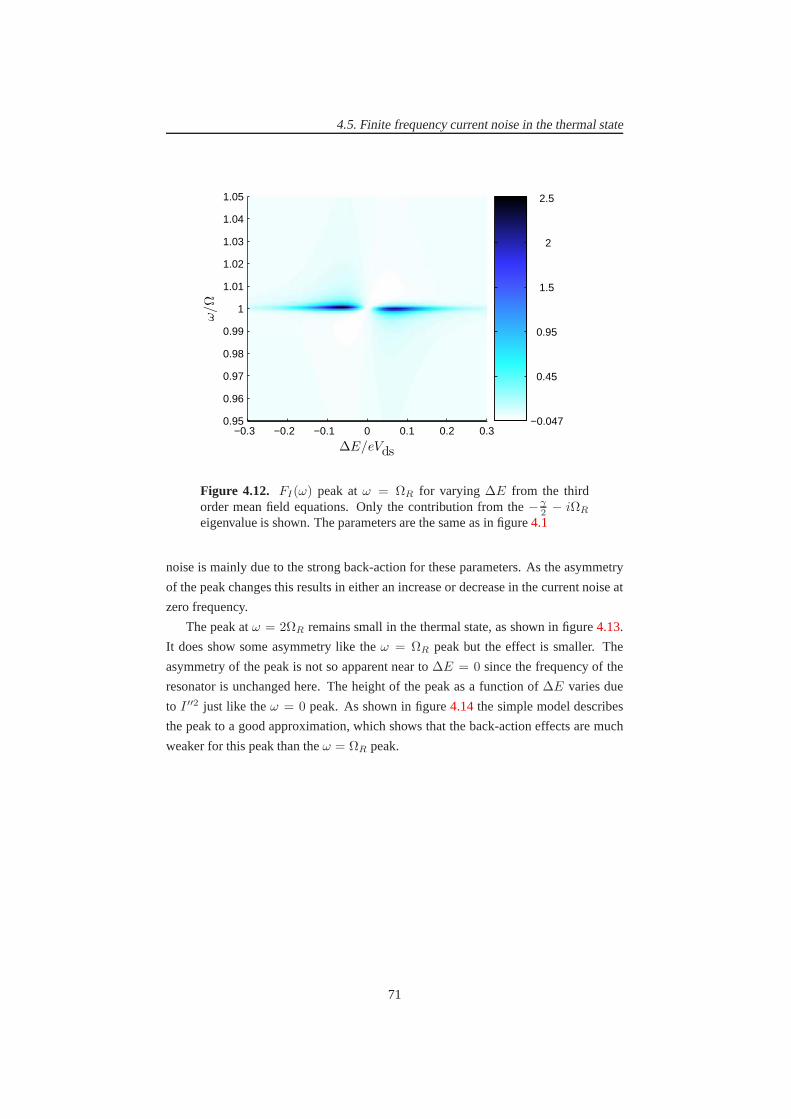
4.5. Finite frequency current noise in the thermal state
−0.3 −0.2 −0.1 0 0.1 0.2 0.30.95
0.96
0.97
0.98
0.99
1
1.01
1.02
1.03
1.04
1.05
∆E/eVds
ω/Ω
−0.047
0.45
0.95
1.5
2
2.5
Figure 4.12. FI(ω) peak atω = ΩR for varying ∆E from the thirdorder mean field equations. Only the contribution from the−γ
2 − iΩR
eigenvalue is shown. The parameters are the same as in figure4.1
noise is mainly due to the strong back-action for these parameters. As the asymmetry
of the peak changes this results in either an increase or decrease in the current noise at
zero frequency.
The peak atω = 2ΩR remains small in the thermal state, as shown in figure4.13.
It does show some asymmetry like theω = ΩR peak but the effect is smaller. The
asymmetry of the peak is not so apparent near to∆E = 0 since the frequency of the
resonator is unchanged here. The height of the peak as a function of ∆E varies due
to I ′′2 just like theω = 0 peak. As shown in figure4.14the simple model describes
the peak to a good approximation, which shows that the back-action effects are much
weaker for this peak than theω = ΩR peak.
71

4.5. Finite frequency current noise in the thermal state
−0.3 −0.2 −0.1 0 0.1 0.2 0.31.98
1.985
1.99
1.995
2
2.005
2.01
2.015
2.02
∆E/eVds
ω/Ω
−2e−005
0.00035
0.00071
0.0011
0.0014
0.0018
Figure 4.13. FI(ω) peak atω = 2ΩR for varying ∆E from the thirdorder mean field equations. Only the contribution from the−γ − 2iΩR
eigenvalue is shown. The parameters are the same as in figure4.1
1.98 1.99 2 2.01 2.020
0.2
0.4
0.6
0.8
1
1.2
1.4
1.6
1.8
2x 10
−3
ω/Ω
FI(ω
)−
Fκ=
0
I(ω
)
mean31
4I ′′2Sx2,x2(ω)
Figure 4.14. Peak atω = 2ΩR comparing the−γ − 2iΩR term fromthe third order mean field equations (mean3) with the corresponding termfrom the simple model (14I ′′2Sx2,x2(ω)) at∆E = 0 with the other param-eters the same as in figure4.1.
72

Chapter 5
Transitions in the Dynamical
State of the Resonator
In Chapter4 we investigated the regime of weak coupling, where the resonator re-
mained in a thermal state, and found that the features seen inthe current noise could
be understood entirely. In this chapter we no longer restrict ourselves to weak cou-
pling and investigate the regime where the SSET drives the resonator into states of
self-sustained oscillations. We focus mainly on the zero frequency current noise, in
particular, we discuss the transition regions in detail.
In Section5.1we give a brief review of transitions that occur and the typesof states
for the three frequency regimes of interest by looking at plots of the current and current
noise. It will become apparent that the current noise in the bistable state is particularly
simple. The noise properties of a generic bistable system are given in Section5.2.
The results of Section5.2 are applied to our system in Section5.3 to show that we
have a true bistability for certain choices of the parameters. The quantum trajectories
method (described in AppendixB) can be used to model an experiment on an individual
quantum system. In Section5.4 this method is applied to the SSET-resonator system.
Finally in Section5.5we generalise some of the results from the bistable transition to
better understand the current noise at the continuous transition and in the limit cycle
state. In doing so we form a better understanding of the eigenfunction expansion of the
Liouvillian.
5.1 A review of the behaviour of the system for moder-
ate coupling
In this section we review the behaviour of the system in the three frequency regimes by
calculating the current and current noise for some typical parameters as a function of
73

5.1. A review of the behaviour of the system for moderate coupling
−1.5 −1 −0.5 00
0.05
0.1
0.15
0.2
0.25
∆E/eVds
〈I〉/
eΓ
Ω = 0.12ΓΩ = ΓΩ = 10Γ
Figure 5.1. Current as a function of∆E for different resonator frequen-ciesΩ/Γ = 0.12, 1, 10. In each case the values ofκ andγext have beenchosen to ensure that the system reaches the limit cycle state for at leastsome values of∆E whilst still remaining at low enough energies to al-low a numerical calculation. ForΩ = 0.12 Γ, κ = 1.5 × 10⁻³ andγext = 1×10⁻⁴ Γ; for Ω = Γ, κ = 5×10⁻³ andγext = 8×10⁻⁴ Γ; andfor Ω = 10 Γ, κ = 3×10⁻³ andγext = 3×10⁻⁴ Γ. The other parametersare the same throughout:EJ = 1/16 eVds, r = 1 andnext = 0.
the detuning. We do this for moderate coupling, by which we mean that the parameters
are such that the resonator is driven into the limit cycle state for ∆E < 0 but the
coupling is insufficient to form any of the more complex states such as the multiple
limit cycles discussed in Section3.7. The current is shown in figure5.1 for resonator
frequencies ofΩ = 0.12 Γ, Ω = Γ andΩ = 10 Γ. The current forΩ = 10 Γ and
Ω = 0.12 Γ are slices through the 2D plots in figures3.8and3.12respectively.
For Ω = 10 Γ the current is almost unmodified around the JQP peak and on the
scale of the plot can be taken as the uncoupled current, when considering the other fre-
quency regimes. At∆E ≃ −1.55 eVds the resonance corresponding to the absorption
of one photon per Cooper pair tunnelling is observed. The resonator is in a limit cycle
state near to the resonance, which is reached via a continuous transition on either side.
ForΩ = 0.12 Γ the current is suppressed near to resonance and enhanced forlarger
negative detuning. This behaviour is the same as seen for theweak coupling case
in Chapter4, but the change is much larger, particularly for∆E < 0. For negative
detuning the resonator is in a limit cycle state in the regionwhere the current is seen
to be strongly modified (the location of the transition will become clearer shortly).
The transition between the fixed point and limit cycle statesoccurs via a continuous
74

5.1. A review of the behaviour of the system for moderate coupling
−0.2 −0.1 0 0.1 0.2 0.30
50
100
150
200
250
300
350
∆E/eVds
FI(0
)
−0.2 −0.15 −0.1 −0.05 0 0.050
10
20
30
40
50
numappapp5+F κ=0
I (0)
Figure 5.2.FI(0) for Ω = 0.12 Γ, with the other parameters given in fig-ure5.1. The curve labellednumshows the numerical value of the noise,app is the approximate value of the noise using the first term in equa-tion 5.3.2, andapp5+Fκ=0
I (0) is the first five terms plusFI(0) for anuncoupled SSET (equation5.5.2).
transition for∆E ≃ 0 and a bistable transition at∆E ≃ 0.12 eVds. The current is
also modified on the positive detuning side but the change is much smaller and so not
apparent in figure5.1. The state of the resonator on the∆E > 0 side is thermal and so
the models of Chapter4 can be applied.
For Ω = Γ the JQP current is strongly altered for∆E < 0. There is a strong
suppression of the JQP peak and peaks are seen correspondingto the1, 2 and3 photon
resonances. The resonator is driven into a limit cycle stateon the∆E < 0 side. Similar
to theΩ = 0.12 Γ case this transition occurs via a continuous transition at∆E ≃ 0. A
bistable transition is then seen at∆E ≃ −0.5 eVds corresponding to a sharp change in
the current.
Figures5.2–5.4show the current noise calculated numerically for the same param-
eters. ForΩ = 0.12 Γ andΩ = Γ the two peaks in the current noise correspond in
both cases to a continuous transition from a fixed point stateto a limit cycle at∆E ≃ 0
and the presence of a region of bistability near the second (larger) peak inFI(0). In
between these two peaks the system is in a limit cycle state. For theΩ = 10 Γ case the
two peaks inFI(0) both correspond to continuous transitions (from fixed pointto limit
cycle state) with the resonator in a limit cycle state between the peaks. Also shown on
the plots are various approximations to the current noise that are introduced later in this
chapter.
75

5.1. A review of the behaviour of the system for moderate coupling
−0.5 −0.4 −0.3 −0.2 −0.1 0 0.10
1
2
3
4
5
6
7
8
9
10x 10
5
∆E/eVds
FI(0
)
−0.4 −0.2 00
10
20
30
40
numappapp5+F κ=0
I (0)
Figure 5.3. FI(0) for Ω = Γ, with the other parameters given in fig-ure5.1. The curve labellednumshows the numerical value of the noise,app is the approximate value of the noise using the first term in equa-tion 5.3.2, andapp5+Fκ=0
I (0) is the first five terms plusFI(0) for anuncoupled SSET (equation5.5.2).
−1.5 −1 −0.5 00
50
100
150
200
250
∆E/eVds
FI(0
)
−1.8 −1.7 −1.6 −1.5 −1.40
2
4
6
8
10
numappapp5+F κ=0
I (0)
Figure 5.4. FI(0) for Ω = 10 Γ, with the other parameters given in fig-ure5.1. The curve labellednumshows the numerical value of the noise,app is the approximate value of the noise using the first term in equa-tion 5.3.2, andapp5+Fκ=0
I is the first five terms plusFI(0) for an uncou-pled SSET (equation5.5.2).
76
5.2. A model of a generic bistable system
5.2 A model of a generic bistable system
The current noise for bistable regions in nanoelectromechanical systems, such as the
charge shuttle, have been studied extensively [88–91]. Before discussing the bistable
region for the SSET-resonator system we describe, in this section, the features of a
generic system that has two current states. This generic bistable system is truly bistable
in the sense that there are only two accessible internal states as opposed to the SSET-
resonator system, where this can only ever be approximatelytrue. The current char-
acteristics of a bistable system can be described by a model specified in terms of four
parameters, which are the currents associated with the two statesI1 andI2, and the
switching rates between them ofΓ12 andΓ21. The current and current noise for this
two-state model take the simple form [90, 92],
〈I〉bi =Γ21I1 + Γ12I2
Γ21 + Γ12, (5.2.1)
SbiI,I(ω) =
4⟨
I2⟩
(Γ21 + Γ12)
ω2 + (Γ21 + Γ12)2, (5.2.2)
where⟨
I2⟩
= Γ21Γ12(I1 − I2)2/(Γ21 + Γ12)
2, is thevariance in the steady-state
current. It is helpful here to make a distinction between thevariance of the current and
the current noise. The variance of the current is the second cumulant of the steady-state
current. The zero frequency current noise on the other hand is the zero frequency limit
of the spectrum of current fluctuations. The latter includesinformation about dynamics
of the system since it considers correlations in the currentat two times.
The simple two-state model can be applied to a more complex system if it can
be described by two metastable states that are well enough separated such that the
switching rate between the states is much slower than the other relevant time-scales [90,
91]. From equation5.2.2we can see how slow switching rates between the two states
can lead to a large value for the current noise in this regime.However, we also note
that when the two metastable states give rise to very different currents the large variance
that results can also make an important contribution to the current noise.
To test the applicability of the simple two state model we canuse the current and
zero frequency current noise together with estimates of thecurrent in the two states to
calculate the switching rates from equations5.2.1and5.2.2. In order to confirm that
the model then works we need a third expression. The current noise involves a two
time correlation function of the current. We can extend thisto higher orders and define
a three time current correlation function. Calculating a double Fourier transform over
this correlation function will result in the third order current noise,
S3I (ω1, ω2) = lim
t→∞
∫ ∞
−∞
dτ1
∫ ∞
−∞
dτ2
⟨
I(t + τ2), I(t + τ1), I(t)⟩
eiω1τ1eiω2τ2 ,
(5.2.3)
77
5.3. Proving the presence of a bistability
where· , · , · is the symmetrized combination of the three operators. The result will
in general depend on two frequencies and although calculable the interpretation is dif-
ficult [93]. Here we require only the zero frequency limit of the the third order current
noise, which we will denote〈〈I3〉〉 following the notation of [90].
〈〈I3〉〉 = limω1→0ω2→0
S3I (ω1, ω2) (5.2.4)
Just likeSI,I(0), 〈〈I3〉〉 is independent of the junction, at which it is measured. For a
bistable system〈〈I3〉〉bi is given by [90, 92],
〈〈I3〉〉bi =6⟨
I2⟩
(I1 − I2)(Γ12 − Γ21)
(Γ21 + Γ12)3. (5.2.5)
Agreement between the bistable model and a calculation of〈〈I3〉〉 provides good evi-
dence that the system is bistable [90].
Another prediction of equation5.2.2is that the finite frequency current noise peak,
atω = 0 is a Lorentzian of widthΓ21 + Γ12. The presence of such a feature provides
further evidence of a bistability [91, 94].
5.3 Proving the presence of a bistability
In this section we use the methods developed in the previous section in order to prove
the presence of a bistability in the SSET-resonator system.We then go on to show how
this relates to the eigenvalue expansion of the current noise. The required parameters
for the two state model can be extracted numerically as follows. The relative probabili-
ties of the two statesΓ21/(Γ21 +Γ12) andΓ12/(Γ21 +Γ12) are obtained by inspection
of the steady state probability distributionP (n). Setting those elements of the steady
state density matrix, which correspond to just one of the twostates, to zero and recal-
culating the current then allows the currentsI1 andI2 to be obtained. Finally, the sum
of the ratesΓ12 +Γ21, and hence the individual rates, can be determined by comparing
the current noise (calculated numerically) with equation5.2.2.
To calculate〈〈I3〉〉 we use the result given in [90], which is valid for the right hand
junction,
〈〈I3R〉〉 = 〈〈l0|IR |r0〉〉 − 6 〈〈l0|IRR(0)IR |r0〉〉 + 6 〈〈l0| IRR(0)IRR(0)IR |r0〉〉
− 6 〈〈l0|IRR(0)R(0)IR |r0〉〉〈〈l0|IR |r0〉〉 (5.3.1)
whereR(ω) andIR were defined in equations2.6.12and2.7.8respectively. We can
only apply the two state model when two meta-stable states can unambiguously be de-
fined (i.e. theP (n) distribution for the resonator steady state should have twopeaks
78

5.3. Proving the presence of a bistability
−0.51 −0.5 −0.49 −0.48−4
−3
−2
−1
0
1
2
3x 10
10
∆E/eVds
〈〈I3〉〉
(a)
−5 0 5
x 10−7
0
1
2
3
4
5
6
x 104
ωS
I,I
(ω)
(b)num
binumbi
Figure 5.5. Comparison of numerical results (num) with the predictionsfor a bistable system (bi) for Ω = Γ, with the other parameters given infigure5.1. (a) Value of〈〈I3〉〉 as a function of∆E. (b) Finite frequencycurrent noise peak aroundω = 0 for ∆E = −0.497.
with a vanishingly small probability for some range ofn values in between). If this is
not the case then it is not possible to separate the density matrix into parts correspond-
ing to each of the states. Generally we can apply the method whenΩ&Γ. The method
can be applied to the bistable state seen at∆E ≃−0.5 eVds in figure5.3 (Ω = Γ) but
not to the bistable state at∆E ≃−0.12 eVds in figure5.2(Ω=0.12 Γ), where there is
significant overlap between the limit cycle and fixed point states.
In figure 5.5awe compare the value of〈〈I3〉〉 obtained numerically with the two
state model by following the above procedure. It can be seen that the values obtained
for the third cumulant from the full numerical solution and the bistable model are in
agreement. Shown in figure5.5bis the finite frequency current noise peak calculated
numerically atω = 0 (see Section2.7) compared with a Lorentzian given by equa-
tion 5.2.2, for a value of∆E near the middle of figure5.5a, which is also in agreement.
These results show that the simple two state model is valid for this set of parameters.
To better understand the bistable model it is helpful to use the eigenfunction expan-
sion of the current noise (see Section2.7). For the zero frequency current noise at the
left hand junction this is (see equation2.7.7),
SILIL(0) = −4
∞∑
p=1
1
λp〈〈l0|IL |rp〉〉〈〈lp|IL |r0〉〉 . (5.3.2)
For comparison a similar expansion of the variance in the steady-state current, also for
79

5.4. Quantum trajectories
the left hand junction, is,
⟨
IL2⟩
=⟨
I2L
⟩
− 〈IL〉2
=
∞∑
p=1
〈〈l0|IL |rp〉〉〈〈lp|IL |r0〉〉 . (5.3.3)
The variance is given by a sum over the same matrix elements asthe current noise,
but this time unmodified by the eigenvalues,λp. Each of the eigenvectors of the Li-
ouvillian |rp〉〉 describe a change to (or fluctuation away from) the steady state that
decays with a purely exponential rate−Re(λp) (see equation2.5.3). Thus, the matrix
element〈〈l0|IL |rp〉〉〈〈lp|IL |r0〉〉 can be thought of as thevariance in the current due
to a fluctuation of typep. We then see that the current noise consists of a sum over
the variances due to each type of fluctuation, each divided bythe rate at which that
fluctuation decays.
It is clear from equation5.3.2that if |λ1|≪ |λ2|, then we expect the current noise
to be dominated by the first term, which corresponds to the slowest time-scale in the
system. This is in indeed what happens when the system has a well-defined bista-
bility. In this case an obvious connection can be made with the two state model de-
scribed in Section5.2 (i.e. equation5.2.2). The smallest eigenvalue corresponds to
the sum of the rates−λ1 = Γ12 +Γ21 and the numerator gives the current variance,
〈〈l0|IL |r1〉〉〈〈l1|IL |r0〉〉=⟨
I2⟩
.
The relationship between the two state model and eigenfunction expansion also
extends to the finite frequency current noise. The first term of the expansion of the finite
frequency current noise at the left hand junction is (see equation2.7.7and discussion
below equation4.5.1),
S1IL,IL
(ω) = − 4λ1
λ21 + ω2
〈〈l0|IL |r1〉〉〈〈l1|IL |r0〉〉 (5.3.4)
Using−λ1 = Γ12 +Γ21 and〈〈l0|IL |r1〉〉〈〈l1|IL |r0〉〉 =⟨
I2⟩
this is identical to equa-
tion 5.2.2.
Although we have used the current noise at the left hand junction here an identi-
cal result can be obtained for the right hand junction. This is becauseSIL,IL(0) =
SIR,IR(0) so if a single term of the expansion describesSIL,IL
(0) then we must have
〈〈l0|IL |r1〉〉〈〈l1|IL |r0〉〉 = 〈〈l0|IR |r1〉〉〈〈l1|IR |r0〉〉. The2e 〈I〉 part ofSIR,IR(ω) can
be neglected when the current noise is large.
5.4 Quantum trajectories
In an experiment, on the SSET-resonator system in the bistable regime, one would hope
to be able to monitor the current with sufficient time resolution to observe the slow
80
5.4. Quantum trajectories
switching between two distinct values of the current directly. By using the method of
quantum trajectories we can model what might occur in an ideal experiment [32, 95,
96].
A full description of the method is given in AppendixB. The basics of the method
are that we have an ideal detector that can detect when a quasi-particle tunnels across
the right hand junction. By use of the quantum trajectories method we can obtain a
density matrix conditioned on a particular measurement record (i.e. the times at which
detections are made). The measurement record could be obtained from an experiment
but, as described in the appendix we can make use of random numbers to perform a
simulation. We will first use the example of a SSET alone to illustrate how information
is gained about the system based on the detection of quasi-particles.
In figure5.6awe show the values of〈p1〉t and〈p2〉t for the beginning of a typical
trajectory. We assume that the experiment is set up att = −∞ and then the detector is
switched on att = 0 so that the initial density matrix is the steady-state density matrix
of the system. The probabilities for the two states are initially the same, since this is
the case for a steady-state. Then over time the probability to be in the|1〉 state rapidly
decays. The reason for this is that there is no way of accessing the|1〉 state except for
a quasi-particle tunnelling and so unless a quasi-particleis detected the probability of
this state must decay away. The probability for the|2〉 state shows strongly damped os-
cillations before coming to a steady value. These oscillations are due to the Josephson
coupling between the|0〉 and|2〉 states and are damped by the quasi-particle tunnelling.
At t = 19.2 Γ a quasi-particle is detected. The detection of a quasi-particle tun-
nelling event corresponds to a rapid change in our knowledgeof the state of the system.
Before the quasi-particle tunnelled across the junction the SSET must have been either
in the |1〉 or the|2〉 state (see figure2.5). After the quasi-particle tunnelling the SSET
must now be either in the|0〉 or the |1〉 state. The expectation values of the charge
states are changed according to,
〈p0〉t+dt =〈p1〉t
〈p1〉t + 〈p2〉t, 〈p1〉t+dt =
〈p2〉t〈p1〉t + 〈p2〉t
, 〈p2〉t+dt = 0, (5.4.1)
where the terms on the bottom ensure the density matrix remains normalized. Since
before the jump〈p1〉t was small the SSET is most likely in the|1〉 state following
the first jump. A second quasi-particle is detected a short time later (t = 20.4 Γ).
Following the second jump the SSET is most likely to be in the state |0〉 state since
before the jump〈p1〉t was large. In between the pairs of quasi-particles we again see
strongly damped oscillations of〈p2〉t due to the Josephson effect, which are strongly
damped due to the large dissipation.
It can be seen in figure5.6athat after detecting a small number of quasi-particles
we can be sure of when the SSET is in the|1〉 state and when it is in a superposition
of the |0〉 and|2〉 states. In a more realistic experiment we should also include things
81

5.4. Quantum trajectories
0 50 1000
0.02
0.04
0.06
0.08
0.1
0.12
t/Γ
(a)
0 50 1000
0.02
0.04
0.06
0.08
0.1
0.12
t/Γ
(b)
0 50 100−15
−10
−5
0
5
10
15
t/Γ
〈x〉 t/
xfp
(c)
0 50 10085
85.5
86
86.5
87
87.5
t/Γ
〈n〉 t
(d)
0.1〈p1〉t〈p2〉t
0.1〈p1〉t〈p2〉t
Figure 5.6.Quantum trajectories: (a)〈p1〉t and〈p2〉t for SSET alone, (b)〈p1〉t and〈p2〉t with resonator, (c) and (d)〈x〉t and〈n〉t for the same tra-jectory as (b). Parameters for (a) are∆E = −0.15 eVds, EJ = 1/16 eVds
andr = 1. Parameters for (b–c) are∆E = −0.45 eVds, κ = 0.005,Ω = Γ, EJ = 1/16 eVds, γext = 8 × 10⁻⁴ Γ, r = 1 andnext = 0.
such as the efficiency of the detector [97], which would lead to some uncertainty in the
state of the SSET.
The method can be extended to include the resonator as well. We could assume that
each photon or phonon that is absorbed and emitted by the resonator can be detected.
For a superconducting stripline resonator the main loss mechanism is through the ca-
pacitors at the ends of the resonator so this detection mightbe feasible experimentally.
For a mechanical resonator, however, the losses cannot be detected and so this would be
an unrealistic model. We therefore assume that we have the same detector but the evo-
lution now includes the resonator also. Calculating the expectation values of resonator
operators will tell us the information we have gained about the state of the resonator
from the detection of quasi-particles.
82

5.4. Quantum trajectories
In figure5.6bwe again show〈p1〉t and〈p2〉t for the beginning of the evolution but
now with coupling to the resonator. For the parameters chosen the resonator is in a limit
cycle state.〈p1〉t behaves as before by initially going rapidly to zero and between the
two quasi-particle tunnellings during each cycle to a valueof one. However,〈p2〉t now
shows continual oscillations rather than the strongly damped oscillations observed in
the uncoupled case. These oscillations become more apparent following the detection
of the quasi-particles. We can understand this from the nature of the coupling in the
device. The charge of the island is coupled to the position ofthe oscillator. The res-
onator therefore oscillates about a different fixed point depending on the charge of the
island. Any knowledge we gain about the island charge must therefore give us some
information about the position of the resonator. As seen in figure5.6c〈x〉t is initially
zero since we have no knowledge about the phase of the oscillator. From the initial
changes in the island charge we gain some knowledge about thephase of the resonator
so we see oscillations in〈x〉t. The position of the resonator modifies the detuning of the
SSET so the oscillations are also present in〈p2〉t. Following the detection of a quasi-
particle we see much larger oscillations in the〈x〉t since we gain additional knowledge
about the phase of the oscillations due to our increased knowledge of the charge. Fi-
nally we can investigate the average energy of the resonatorshown in figure5.6d. For
these parametersnext = 0 so the resonator can only gain energy from the SSET. We
therefore observe an initial decay of〈n〉t. The current through the SSET here would
be almost zero in the absence of coupling to the resonator so following the detection
of the first quasi-particle in the cycle it is very likely thatsome energy is transferred
from the SSET to the resonator. We therefore see a jump in the energy following the
detection of the first quasi-particle but not the second since this does not give us any
further information.
We now investigate the case of a bistable region. The currents for the limit cycle
and fixed point states are very different, which leads to a large variance in the overall
current as seen in the previous sections. In terms of the trajectories, the limit cycle state
has higher energy than the fixed point state, which must be sustained by the detection
of a large number of quasi-particles. Conversely for a fixed point state there must be a
sufficient gap between tunnelling events in order for the resonator to relax. The limit
cycle state is therefore the state with the higher current. The two states here are less
well separated here than the bistability we studied in Section 5.3. The reason being
that numerical time evolution is slow and needs to be carriedout for a long enough
time that a large number of switches between the fixed point and limit cycle occur. In
figure5.7awe show the evolution of〈n〉t for these parameters and the associatedP (n)
distribution in figure5.7b. The value of〈n〉t spends time mainly aroundn = 0 and
n = 25, which correspond to the peaks in theP (n) distribution, this confirms that the
quasi-particle detection tells us when the resonator is in the fixed point or limit cycle
states.
83

5.4. Quantum trajectories
0 5 10
x 104
0
5
10
15
20
25
30
35
40
45
t/Γ
〈n〉 t
(a)
0 10 20 30 40 500
0.05
0.1
0.15
0.2
0.25
0.3
0.35
nP
(n)
(b)
Figure 5.7. (a) Quantum trajectory of〈n〉t for bistable region. (b) Asso-ciatedP (n) distribution. Parameters are∆E = −0.473 eVds, κ = 0.016,Ω = Γ, EJ = 1/16 eVds, γext = 0.003 Γ, r = 1 andnext = 0.
The trajectory of〈n〉t can be used to calculate the waiting times in the limit cycle
and fixed point states and hence calculate the switching rates between the two. As seen
in figure5.7ait is not always clear which state the system is in. By choosing a better
separated bistable state the situation is improved, however, the tunnelling rate between
the two states can then become very slow and so the length of time taken to simulate
the trajectory is too long. First the centre of each state is determined, either from the
P (n) distribution or estimated from the trajectory. The system is then said to have
entered the state when〈n〉t passes this mid-point.
The tunnelling rate out of a state is given by the inverse of the average time the
system spends in the state. Adding up the number of quasi-particles detected while in
each state gives an estimate of the current in each of the states. This provides another
method of determining the rates and currents in equations5.2.1and5.2.2. Using the
parameters in figure5.7we obtain the following results from the trajectories.
I1 = 0.0127 I2 = 0.049
Γ12 = 6.99 × 10⁻⁵ Γ21 = 5.13 × 10⁻⁵ (5.4.2)
Then by use of equations5.2.1and5.2.2we can calculate,
〈I〉bi = 0.034 SbiI,I(0) = 10.66
Γ12 + Γ21 = 1.21 × 10⁻⁴ (5.4.3)
84

5.5. Transitions and time-scales
The numerically obtained values are,
〈I〉 = 0.033 SI,I(0) = 14.5
−λ1 = 1.20 × 10⁻⁴ (5.4.4)
The bistability here is not sufficiently good to get the correct current noise but we obtain
good agreement for the current and between the eigenvalue and sum of the switching
rates.
5.5 Transitions and time-scales
In general, we cannot describe our system in the vicinity of the dynamical transitions
by a simple two-state model. As we have seen, even where the transition involves a
region of coexistence between the limit cycle and fixed pointstates the states may not
be well enough separated for a two-state model to apply. Nearthe continuous transi-
tions between the limit cycle and fixed point states there areclearly not just two states
involved. However, one element of the two state model which might be expected to
apply more widely is the emergence of a single very slow time-scale, which dominates
the current noise. In the case of the continuous transition such a slow time-scale might
result from the vanishing effective damping (γsset+γext) of the system at the transition.
In what follows we use the eigenfunction expansion of the Liouvillian to investigate the
extent to which the current noise can be described by a singleterm of this expansion.
More generally, it is not just a slow time-scale that is important. For a single term
in the eigenfunction expansion (equation5.3.2) to accurately describe the noise, the
matrix element divided by the eigenvalue〈〈l0|IL |rp〉〉〈〈lp|IL |r0〉〉 /λp for p = 1 must
be much larger than for allp ≥ 2. In figures5.2–5.4 we compare the full current
Fano factor with approximations using just the first term in equation5.3.2. The peaks
at the transitions are described quite well by just the first term in the eigenfunction
expansion. Away from the peaks, however, we find that the noise is not captured by
the approximation based on the first term. It is particularlyclear in figure5.4 that
something is missing from this approximation. The featuresthat are simply due to
the SSET alone are not captured, such as the dip at∆E = 0 and the Fano factor
of 2 far from resonance. We can understand this better by considering the meaning
of the eigenvectors and eigenvalues of the Liouvillian [64, 86]. The meaning of the
eigenvalues when the resonator can be described by a thermalstate was previously
discussed in Chapter4. We repeat some of this here for clarity.
In the limit κ → 0 the SSET-resonator system becomes uncoupled and the eigen-
vectors and eigenvalues of the system can be expressed in terms of those of the indi-
vidual subsystems, namely the SSET and the resonator. When the resonator is decou-
85

5.5. Transitions and time-scales
pled from the SSET it still remains coupled to the external bath and its smallest (non-
zero) eigenvalues are integer multiples ofγext (Section4.3) [86]. Thus the smallest of
these eigenvalues corresponds to the energy relaxation rate of the resonator,−γext, and
hence we can infer that the corresponding eigenfunction describes fluctuations in the
resonator’s energy. There are also a set of eigenfunctions (and corresponding eigenval-
ues) that describe fluctuations in the SSET charge state. In the uncoupled regime the
current noise of the SSET can be obtained using equation5.3.2, with the sum running
over just the SSET eigenvalues, though we already know the result will be given by
equation3.2.2.
For the coupled SSET-resonator system we can still identifythe eigenvalues and
eigenvectors as corresponding to one or other of the subsystems by looking at their
behaviour for large detunings (i.e. large|∆E|) where the systems are effectively de-
coupled. The first few eigenvalues, which correspond to the resonator, are shown (for
the slow resonator caseΩ=0.12 Γ) in figure5.8as a function of∆E. These first few
eigenvalues indeed converge towards−γext, −2γext, . . . for large detunings. Thus at
least for large detunings the first eigenstate,|r1〉〉, should therefore represent fluctu-
ations which change the resonator energy. This can be confirmed by performing an
eigenfunction expansion of the variance in the resonator energy,
⟨
n2⟩
=∑
p=1
〈〈l0|N |rp〉〉〈〈lp|N |r0〉〉 , (5.5.1)
whereN |ρ(t)〉〉 ≡ nρ(t) = a†aρ(t). As before we plot the resonator Fano factor,
Fn =⟨
n2⟩
/ 〈n〉, rather than the variance. The full numerical calculation of the energy
variance is compared with approximations based on the first term and first 5 terms in
the eigenfunction expansion in figure5.9. It is clear that only the first term is needed
to describe the energy fluctuations for large detunings as weexpect. However, the
approximation based on the first term also describes the energy fluctuations rather well
at the peaks where the transitions occur, but not in between where the resonator is in
a limit cycle state. However, figure5.9 also shows that we can describe the energy
fluctuations throughout by using more terms in the eigenfunction expansion.
We are now in a position to understand why the calculation of the current noise
using just the first term of the eigenvector expansion works as well as it does and to see
how this can be easily improved upon. Comparing figures5.2 and5.9 it is clear that
the single-term approximation to the current noise matchesthe numerical results well
around the two peaks marking the transitions (between the fixed point and limit cycle
states) where the first term in the eigenfunction expansion also describes the energy
fluctuations in the resonator accurately. The fact that the first term in the expansion
does not capture the current noise far from resonance is not surprising as it only de-
scribes fluctuations in the resonator state and does not include the fluctuations of the
86

5.5. Transitions and time-scales
−0.3 −0.2 −0.1 0 0.1 0.2 0.30
2
4
6
8
10
12
14
∆E/eVds
−λp/γex
t
−0.2 0 0.2−2
−1
0
1
2
Figure 5.8. The five smallest (non-zero) eigenvalues as a function of thedetuning,∆E for Ω = 0.12 Γ, with the other parameters given in fig-ure5.1. The inset showslog10(−λp/γext). The eigenvalues differ fromeach other by less than one order of magnitude throughout andconvergetowards integer multiples ofγext for large|∆E|.
−0.2 −0.1 0 0.1 0.2 0.30
5
10
15
20
25
30
35
∆E/eVds
Fn
−0.2 −0.15 −0.1 −0.05 0 0.050
2
4
6
8
10
num
app
app5
Figure 5.9. Energy fluctuations of the resonator,Fn, as a function of∆E for Ω = 0.12 Γ, with the other parameters given in figure5.1. Thethree curves show the full numerical calculation,num, and approxima-tions using just the first term,app and the first five terms,app5, of theeigenfunction expansion (equation5.5.1) respectively.
87

5.5. Transitions and time-scales
SSET degrees of freedom. We can easily obtain better agreement for large detunings
by extending our approximation to include the contributionof an uncoupled SSET,
Fκ=0I (0), given by equation3.2.2. Better agreement within the limit cycle region can
be attained by using sufficient terms in our approximation toensure that the fluctu-
ations in the resonator energy are described accurately. Thus we arrive at our final
approximate expression for the zero frequency current noise
FI(0) ≃ Fκ=0I − 2
m∑
p=1
〈〈l0|IL |rp〉〉〈〈lp|IL |r0〉〉λpe 〈I〉
, (5.5.2)
wherem should be large enough so that the corresponding number of terms can be
used to calculate⟨
n2⟩
accurately (via equation5.5.1). In this case we findm = 5 is
sufficient, and the current noise calculated this way agreesvery well at almost all points
as shown in figures5.2–5.4. The one area where good agreement is still lacking using
equation5.5.2is within the limit cycle region forΩ = 10 Γ, shown in figure5.4. This
is because we have approximated the contribution to the current noise arising from the
SSET terms by the uncoupled value. In fact these SSET terms are strongly modified
due to the resonant absorption of energy by the resonator from the Cooper pairs at this
point.
From these approximations it is clear that in the vicinity ofthe resonator transitions
the current noise is largely determined by the slow fluctuations in the energy of the
resonator. This is because the current depends in the first instance on the resonator
position and hence on the latter’s energy (as this is slowly changing compared to its
period). Thus the current fluctuations depend strongly on the fluctuations of the res-
onator energy, rather than those of higher moments of the resonator. Thus when⟨
n2⟩
depends on more than one term in the expansion, the current noise does also.
It is important to note that even in the regions where including just the first term
in the eigenfunction expansion describes the current noisefairly well this is not simply
because the associated eigenvalue is very much smaller thanall the others. We can
see from figure5.8that (for these parameters) an overwhelming difference between the
slowest two eigenvalues never develops and from figure5.10, that the relative size of
the corresponding matrix elements is important in causing the first term in the eigen-
function expansion to dominate.
The other frequency regimes also show interesting featuresin the expansion of the
resonator Fano factor. As shown in figure5.11we again require more than one term to
fully describeFn in the limit cycle region for the case ofΩ=Γ. In the low frequency
regime (figure5.9) there was a smooth deviation of the one term approximation from
the actual value in the limit cycle region. In the inset of figure5.11it is clear that instead
there are abrupt changes seen in the one term approximation,at∆E ≃ −0.2 eVds and
also just to the right of∆E = 0. Note that these changes are also seen in the one term
88

5.5. Transitions and time-scales
−0.2 −0.1 0 0.1 0.2 0.3−0.5
0
0.5
1
1.5
2
2.5
3x 10
−4
∆E/eVds
〈〈l0|I
L|r p
〉〉〈〈l p|I
L|r 0
〉〉
p=1p=2p=3
Figure 5.10. Variance part of the current noise for the first 3 terms ofthe expansion (equation5.3.2) for Ω = 0.12 Γ, with the other parametersgiven in figure5.1. Thep = 1 variance is much larger in the same regionsas the peaks in the corresponding plot of the current noise, figure5.2.
approximation of the current noise, although they cannot beclearly seen in figure5.3.
The reason for this can be understood from a plot of the eigenvalues that correspond
to the terms used in the expansion. As shown in figure5.12 there are a number of
crossings present in the eigenvalues. There is a crossing at∆E ≃ −0.2 eVds and also
for ∆E > 0 (although less clear). The point at which the single term approximation
fails corresponds exactly to these crossings.
From a plot of the first few terms in the eigenfunction expansion of Fn, which
is shown in figure5.13, it can be seen that for the majority of the limit cycle region
only one term is required. However, this term does not necessarily correspond to the
smallest magnitude eigenvalue. At the crossing for∆E ≃ −0.2 eVds the new smallest
eigenvalue develops into the bistable switching rate and correctly captures the noise
in the bistable region. However, when the system is not bistable it is not the correct
term to describeFn or FI(0). It can be seen from figures5.12and5.13that it is the
same eigenvalue that leads to the correct single term approximation toFn but that it
undergoes a number of crossings.
For the case ofΩ = 10 Γ, as shown in figure5.14, the smallest eigenvalue is
sufficient to captureFn except for near to the transitions. The eigenvalues do not cross
at this point, as shown in figure5.15, but the smallest two become close. During the
transition region the first few terms have an important contribution. The one term
approximation to the current noise at the transition was still quite good since the first
89
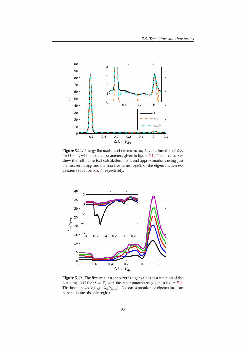
5.5. Transitions and time-scales
−0.5 −0.4 −0.3 −0.2 −0.1 0 0.10
10
20
30
40
50
60
70
80
90
100
∆E/eVds
Fn
−0.4 −0.2 00
1
2
3
4
num
app
app5
Figure 5.11.Energy fluctuations of the resonator,Fn, as a function of∆Efor Ω = Γ, with the other parameters given in figure5.1. The three curvesshow the full numerical calculation,num, and approximations using justthe first term,appand the first five terms,app5, of the eigenfunction ex-pansion (equation5.5.1) respectively.
−0.8 −0.6 −0.4 −0.2 0 0.20
5
10
15
20
25
30
35
40
∆E/eVds
−λp/γex
t
−0.8 −0.6 −0.4 −0.2 0 0.2−6
−4
−2
0
2
Figure 5.12.The five smallest (non-zero) eigenvalues as a function of thedetuning,∆E for Ω = Γ, with the other parameters given in figure5.1.The inset showslog10(−λp/γext). A clear separation of eigenvalues canbe seen in the bistable region.
90

5.5. Transitions and time-scales
−0.5 −0.4 −0.3 −0.2 −0.1 0 0.10
10
20
30
40
50
60
70
80
90
100
∆E/eVds
〈〈l0|N
|r p〉〉〈〈
l p|N
|r 0〉〉
p=1p=2p=3p=4p=5
Figure 5.13.First five terms in the expansion of⟨
n2⟩
(equation5.5.1) forΩ = Γ, with the other parameters given in figure5.1. One term generallydominates but it does not always correspond to the smallest eigenvalue.
term captures most of the peak and the eigenvalues provide a large scaling. The state
of the system during the transition is similar to that in the limit cycle for Ω = 0.12 Γ
where more than one term was also required to describeFn. The state of the resonator
at these points was previously described in Section3.4where a discussion of the state
of the resonator during the continuous transition was made.In these cases theP (n)
distribution consists of a Gaussian like shape with a sharp cut-off at n = 0 due to
the width being larger than〈n〉, an example of which was shown in figure3.9. For
Ω = 10 Γ andΩ = Γ we obtain ’good’ limit cycle states (i.e.P (0) ≃ 0) in the regions
where only one term is required to describeFn. ForΩ = 0.12 Γ this is not the case for
the parameters used here.
In conclusion, for the regimes studied in this chapter, the majority of states of the
system have a value ofFn that can be described by a single term in an eigenfunction
expansion of the Liouvillian. The exception to this is limitcycle states whereP (0) 6≃0. The corresponding term in an eigenfunction expansion of the current noise also
describes the dominant contribution toFI(0) that is different from the current noise of
an uncoupled SSET.
91

5.5. Transitions and time-scales
−1.5 −1 −0.5 01
2
3
4
5
6
7
8
∆E/eVds
Fn
−1.7 −1.575 −1.45
2
4
6
8
num
app
app5
Figure 5.14. Energy fluctuations of the resonator,Fn, as a function of∆E for Ω = 10 Γ, with the other parameters given in figure5.1. Thethree curves show the full numerical calculation,num, and approxima-tions using just the first term,app and the first five terms,app5, of theeigenfunction expansion (equation5.5.1) respectively.
−1.8 −1.7 −1.6 −1.5 −1.40
0.2
0.4
0.6
0.8
1
1.2x 10
−3
∆E/eVds
−λp/γex
t
−1.7 −1.6 −1.5 −1.4−4.5
−4
−3.5
−3
−2.5
Figure 5.15.The five smallest (non-zero) eigenvalues as a function of thedetuning,∆E for Ω = 10 Γ, with the other parameters given in figure5.1.The inset showslog10(−λp/γext).
92

Chapter 6
Finite Frequency Resonator
Noise Spectra
In this chapter we discuss the dynamics of the limit cycle region in some more detail.
In order to do this we make use of several finite frequency noise spectra of resonator
operators. Throughout we make comparisons between the SSET-resonator system and
a laser. In particular we investigate the linewidth of the resonator, which is introduced
in Section6.1. We show that as for a laser the linewidth in the limit cycle region
is dominated by phase diffusion. In Sections6.2 and6.3 we give the results for the
Ω ≫ Γ andΩ ≃ Γ regimes respectively.
6.1 Calculation of the resonator linewidth
The linewidth of a laser,γΩ, is defined as the width of the peak in the emission spec-
trum, at the frequency of the resonator [77]. Above threshold the linewidth of a laser
becomes very narrow indicating an almost monochromatic light source. The emission
spectrum is defined as,
Sa,a†(ω) = limt→∞
∫ ∞
−∞
dτ⟨
a(t + τ), a†(t)⟩
eiωτ . (6.1.1)
The numerical calculation of spectra such as these was described in Section2.6. We
could equally useSa†,a(ω), in the definition of the emission spectrum, since for sym-
metrized noiseSa,a†(ω) = Sa†,a(−ω). We chooseSa,a†(ω), since it has the peak for
ω > 0. The correlation function, in the emission spectrum, corresponds to putting in
a photon at timet then removing it att + τ . The spectrum was measured in the ex-
periment of a SSET coupled to a superconducting stripline resonator [30]. To do this a
small microwave drive was applied to the cavity and the emission from the cavity was
93

6.1. Calculation of the resonator linewidth
measured as the frequency of the drive was varied.
We can identify two sources of noise in the resonator that contribute to the finite
linewidth. These are the amplitude noise and the phase noise. The amplitude noise is
characterized by the amplitude relaxation rate,γn. In the limit cycle region the ampli-
tude noise leads to the finite width of of the ring in the Wignerdistribution (figure3.1b).
The phase noise is characterized by the phase diffusion rate, γφ. In a laser the phase
noise is due to jumps in phase associated with spontaneous emission [77]. The equiva-
lent process in the SSET-resonator system is the energy exchange between the Cooper
pairs and resonator.
The linewidth can depend on one or both of the diffusion rates. In order to show,
on which one it depends it is helpful to be able to calculate the two rates indepen-
dently. The amplitude relaxation rate can be found from the spectrum of amplitude
fluctuations,
Sn,n(ω) = limt→∞
∫ ∞
−∞
dτ 〈n(t + τ), n(t)〉 eiωτ , (6.1.2)
which will have a peak atω = 0 with a widthγn.
In order to calculate the spectrum of phase fluctuations we must first define an
operator for the phase. There is much debate over the correctform for the phase op-
erator [73]. We choose to use the Susskind-Glogower operators [98, 99], which are
valid so long as the occupation of the vacuum state is negligible [73]. This condition is
not restrictive since for a limit cycle state, where the phase is of interest, the condition
must be met. The two operators are analogous to the exponential phase factors,e±iφ,
and are defined,
p ≡ (n + 1)−12 a = (aa†)−
12 a =
∞∑
N=0
|N〉〈N + 1| ,
p† ≡ a†(n + 1)−12 = a†(aa†)−
12 =
∞∑
N=0
|N + 1〉〈N | . (6.1.3)
We define the phase noise spectrum in a similar manner to the emission spectrum,
Sp,p†(ω) = limt→∞
∫ ∞
−∞
dτ⟨
p(t + τ), p†(t)⟩
eiωτ . (6.1.4)
For a laser above threshold the linewidth is dominated by thephase noise [77]. In order
to show that this is also true for the SSET-resonator system we derive a relationship
between the emission and phase noise spectra that is valid for a laser. Under the as-
sumption thatγφ ≪ γn, the amplitude relaxation occurs on a much faster time-scale
than the phase relaxation. If this is true then we can neglectfluctuations in the ampli-
tude and assume that it takes its steady-state value. The following relationship between
94

6.1. Calculation of the resonator linewidth
−15 −10 −5 0 5
x 10−6
0
0.5
1
1.5
2
2.5x 10
9
ω −Ω
Saa†(ω)
〈n〉Spp†(ω)
Figure 6.1. Shows thatSaa†(ω) = 〈n〉Spp†(ω) which means thatamplitude and phase noise are uncorrelated as discussed around equa-tion 6.1.5. Parameters areΩ = 10 Γ, ∆E = −1.58 eVds, κ = 0.003,γext = 3 × 10⁻⁴ Γ, EJ = 1/16 eVds, r = 1 andnext = 0
the emission and phase noise spectra in the limit cycle region can then be derived,
Sa,a†(ω) = limt→∞
∫ ∞
−∞
dτ⟨
(n(t + τ) + 1)1/2p(t + τ), (n(t) + 1)
1/2p†(t + τ)⟩
eiωτ
= limt→∞
∫ ∞
−∞
dτ⟨
〈n〉1/2p(t + τ), 〈n〉1/2
p†(t + τ)⟩
eiωτ
= 〈n〉Sp,p†(ω). (6.1.5)
In the first line we have used the definition of the phase operators given in equa-
tion 6.1.3to replacea anda†. In the second line we have replacedn(t) andn(t + τ)
with the steady-state value,〈n〉, and additionally assumed〈n〉 ≫ 1, which is true for
the limit cycle state. Removing〈n〉 from the integral then leads directly to the final
line. In figure6.1we show the relationship to hold for the SSET-resonator system for
a set of parameters in the limit cycle region. Below we will show in a different manner
that the relationship holds throughout the limit cycle region.
It can also be seen in figure6.1that the peak in the emission spectrum is symmetric.
We would expect this to be the case for all peaks in resonator spectra. The reason for
this is that, as discussed in Section4.5, the asymmetric shape in the current noise peaks
is due to the back-action of the resonator on the SSET. The asymmetry was removed
by the addition of a large external damping or temperature for the resonator. Since the
dissipation in the SSET is large (due to the large value ofΓ in comparison to other time-
95

6.2. Phase Diffusion forΩ ≫ Γ
scales) any back-action effects will be removed and peaks inthe spectra of resonator
operators will be symmetric. A small renormalization of theresonator frequency to the
valueΩR can also be seen in the figure.
6.2 Phase Diffusion forΩ ≫ Γ
In Section5.5we found that the⟨
n2⟩
could be described by a single term of an eigen-
function expansion when the resonator was in a fixed point or good limit cycle state. If
this is true thenSn,n(ω) is also described by a single term in an eigenfunction expan-
sion since the same matrix element part will appear. Where the single term approxima-
tion is valid,Sn,n(ω) will be given by a Lorentzian peak of the form,
Sn,n(ω) = 4ℜ∞∑
p=1
1
−iω − λp〈〈l0|N |rp〉〉〈〈lp|N |r0〉〉
≃ 4ℜ[
1
−iω − λ1
]
〈〈l0|N |r1〉〉〈〈l1|N |r0〉〉
=4⟨
n2⟩
γn
ω2 + γ2n
. (6.2.1)
If the single term approximation is valid then−λ1 = γn and so the amplitude diffusion
rate can be calculated without resorting to a calculation ofthe full spectrum of ampli-
tude fluctuations. In figure6.2we compare the width of theω = 0 peak in theSn,n(ω)
spectrum as determined from a Lorentzian fit to the smallest non-zero eigenvalue of
the Liouvillian. They are in agreement except for around thetransition region where
we do not expect the expansion to work (see Section5.5).
Similarly the peak in the emission spectrum is also likely tobe described by a
Lorentzian with a width determined by the real part of the eigenvalue nearest−iΩ.
The emission spectrum will be of the form,
Sa,a†(ω) = 4ℜ∞∑
p=1
1
−iω − λp〈〈l0|A|rp〉〉〈〈lp|A† |r0〉〉
≃ 4ℜ[
1
−iω − λ1
]
〈〈l0|A|r1〉〉〈〈l1|A† |r0〉〉
=4 〈n〉 γΩ
(ω − ΩR)2 + γ2Ω
. (6.2.2)
whereA |ρ(t)〉〉 = 12 (aρ(t) + ρ(t)a). As shown in figure6.2 the width of the peak in
the emission spectrum is in agreement with the eigenvalue. If the single term approxi-
mation is valid we should also find thatm1e = 〈〈l0|A|r1〉〉〈〈l1|A† |r0〉〉 = 〈n〉, which is
confirmed in figure6.3a. For bothSn,n(ω) andSa,a†(ω) we can also check the size of
the next term in the eigenfunction expansion to ensure that it is small. For the results
96

6.2. Phase Diffusion forΩ ≫ Γ
−1.7 −1.585 −1.47−6.5
−6
−5.5
−5
−4.5
−4
∆E/eVds
log 1
0γ
γn/2 fitγn/2 eigγΩ fitγΩ eig
Figure 6.2. Width of zero frequency peak in theSn,n(ω) spectrum asdetermined from a Lorentzian fit (γn/2 fit) and from the smallest nonzeroeigenvalue (γn/2 eig). Linewidth of the resonator as determined from aLorentzian fit (γΩ fit) and from the eigenvalue (γΩ eig). Parameters arethe same as in figure6.1. Within the pairs of vertical dashed lines theP (n) distribution has a peak atn 6= 0 but P (0) ≥ 1 × 10⁻⁵, which wedefine here as the transition regions.
97

6.2. Phase Diffusion forΩ ≫ Γ
−1.7 −1.585 −1.470
20
40
60
80
100
120
140
160
∆E/eVds
(a)
−1.7 −1.585 −1.470.8
0.85
0.9
0.95
1
1.05
1.1
∆E/eVds
(b)〈n〉
m1e
m1p
Figure 6.3. (a) shows the agreement of〈n〉 andm1e as explained in the
text. (b) showsm1p = 1 and the vertical dashed lines indicate the good
limit cycle region as defined in figure6.2. Parameters are the same as infigure6.1.
in this chapter, unless otherwise stated, this check has been made and the contributions
from other terms can be neglected.
For a thermal state (which is the case away from the resonancepeak) we expect,
from Section4.3, thatγΩ = γn/2. At the edges of figure6.2 it can be seen that this is
indeed the case. Within the limit cycle region there is a separation betweenγn andγΩ
of at least one order of magnitude. Additionally following the transitionγn increases
while γΩ continues to decrease to a minima at the resonance.
Within the limit cycle region we can also perform an eigenfunction expansion of
Sp,p†(ω). Just like forSn,n(ω) andSa,a†(ω) only a single term is required. We obtain,
Sp,p†(ω) = 4ℜ∑
p=1
1
−iω − λp〈〈l0|P |rp〉〉〈〈lp|P† |r0〉〉
≃ 4⟨
pp†⟩
γΩ
(ω − ΩR)2 + γ2Ω
, (6.2.3)
whereP |ρ(t)〉〉 = 12 (pρ(t) + ρ(t)p). Clearly we must haveγΩ = γφ within the limit
cycle region for bothSp,p†(ω) andSa,a†(ω) to be described by a single term in the
expansion. As further confirmation of the relationship in equation6.1 we should also
find thatm1p = 〈〈l0|P |r1〉〉〈〈l1|P† |r0〉〉 =
⟨
pp†⟩
= 1, which is shown in figure6.3b.
Note that the value ofm1p has no meaning outside the limit cycle region.
In figure 6.4 we again showγn andγΩ. Also shown is the real part of the next
closest eigenvalue to−iΩ (labelledγΩ(2)). It can be seen that outside the limit cycle
98

6.2. Phase Diffusion forΩ ≫ Γ
−1.8 −1.7 −1.6 −1.5 −1.40
0.2
0.4
0.6
0.8
1
1.2
1.4
∆E/eVds
−γn/γext−γΩ/γext−γΩ(2)/γext
Figure 6.4. Amplitude relaxation rateγn and the real part of the twoeigenvalues nearest−iΩ, γΩ andγΩ(2). Parameters are the same as infigure6.1
region it approaches the expected value, from Section4.3, of − 32γn. Within the limit
cycle region it is equal toγn. This suggests that this next term in the expansion is the
contribution to the linewidth due to the amplitude noise in the limit cycle, which is
small due to the large separation of the eigenvalues.
For a laser the phase diffusion rate has a particularly simple form [48],
γlaserφ =
G
8 〈n〉 , (6.2.4)
whereG is the gain of the laser. However, it is not entirely clear what the gain is for the
SSET-resonator system and〈n〉 cannot be varied independently from the parameters of
the system, on which the gain will depend. However, we can at least show qualitatively
that there is an inverse relationship between〈n〉 andγφ. In figures6.5and6.6we show
〈n〉 andγφ for varying values ofκ andγext. The detuning is chosen to be at the one
photon resonance in the centre of figure6.2. It can be seen that as〈n〉 increasesγφ
does indeed reduce.
In examining the off-resonant behaviour of〈n〉 andγφ we observe a striking devi-
ation from the expected relationship between the two values. We now fixγext and vary
the detuning about the one photon resonance for a range of coupling strengths. Similar
plots were produced in figure3.8 but here we go to higher coupling strengths. The
value of〈n〉 is shown in figure6.7. For increasing coupling〈n〉 reaches a maximum
and then shows a decrease. The peak also becomes wider for larger coupling as this
99

6.2. Phase Diffusion forΩ ≫ Γ
0.005 0.01 0.015 0.021
1.5
2
2.5
3
3.5
4
4.5
5x 10
−4
κ
γex
t
3.1
39
75
110
150
180
Figure 6.5.Value of〈n〉 as a function of the coupling and external damp-ing with the other parameters given in figure6.1. The green region in thebottom left has no results due to an insufficient number of resonator states.Except for a small strip for largeγext and smallκ (top left) the resonatoris in the limit cycle state.
0.005 0.01 0.015 0.021
1.5
2
2.5
3
3.5
4
4.5
5x 10
−4
κ
γex
t
3.8e−007
1.3e−005
2.5e−005
3.7e−005
4.9e−005
6.2e−005
Figure 6.6. Value of−ℜλΩ as a function of the coupling and externaldamping with the other parameters given in figure6.1. The green regionin the bottom left has no results due to an insufficient numberof resonatorstates. Except for a small strip for largeγext and smallκ (top left) theresonator is in the limit cycle state and so−ℜλΩ = γφ.
100

6.2. Phase Diffusion forΩ ≫ Γ
−1.8 −1.6 −1.4 −1.2
0.005
0.01
0.015
0.02
0.025
0.03
0.035
∆E/eVds
κ
0.035
30
60
90
120
150
Figure 6.7.Value of〈n〉 for varying∆E andκ with the other parametersgiven in figure6.1.
maximum is approached.
In figure 6.8 the value ofFn is shown for the same parameters. Peaks are seen
in Fn at the transitions between fixed point and limit cycle behaviour as discussed in
previous chapters. Beyond the peak in〈n〉 the value ofFn continues to decrease and in
doing so drops below one. This corresponds to a sub-PoissonianP (n), which is also
observed in the micromaser (see Section3.7) but not a conventional laser.
In figure6.9the linewidth,γΩ, as calculated from the eigenvalues is shown. Within
the limit cycle region this can be interpreted asγφ where we focus our attention. The
region in whichγΩ = γφ is indicated in figure6.9. For low coupling the peak in〈n〉corresponds to a minimum inγφ. But for large coupling we see a deviation from this
behaviour. Two minima are seen inγφ with the peak in〈n〉 now corresponding to a
local maximum inγφ.
For the parameters here the single term approximation, given in equation6.2.2,
always describes the peak in the emission spectrum. We show the effect of the changing
eigenvalue on the height of the peak in the emission spectrumin figure6.10. It can be
seen that the increased coupling causes a splitting of the peak in the emission spectrum.
This splitting is not responsible for the double peak seen inthe emission spectrum of
the experiment [30]. In the experiment a matching feature was observed in the current,
which is not the case here (the current follows〈n〉 as discussed in Section3.4). Note
also that the splitting is only as a function of the detuning,there is still just a single
Lorentzian peak in the emission spectrum.
The amplitude relaxation rate, shown in figure6.11, does not show any unexpected
101

6.2. Phase Diffusion forΩ ≫ Γ
−1.8 −1.6 −1.4 −1.2
0.005
0.01
0.015
0.02
0.025
0.03
0.035
∆E/eVds
κ
0.49
2.2
3.9
5.7
7.4
9.1
Figure 6.8. Value ofFn for varying∆E andκ with the other parametersgiven in figure6.1.
−1.8 −1.6 −1.4 −1.2
0.005
0.01
0.015
0.02
0.025
0.03
0.035
∆E/eVds
κ
4.5e−007
1.5e−006
4.8e−006
1.6e−005
5.2e−005
0.00017
Figure 6.9.Linewidth of the resonator,γΩ, for varying∆E andκ with theother parameters given in figure6.1. Colours are on alog10 scale. Withinthe region given by the dashed lines the resonator is in a limit cycle stateandP (0) ≤ 1 × 10⁻⁵ soγΩ = γφ.
102

6.3. Phase Diffusion in theΩ ≃ Γ regime
−1.8 −1.7 −1.6 −1.5 −1.4 −1.3 −1.20
1
2
3
4
5
6
7
8
9
10x 10
8
∆E/eVds
4〈n〉/
γΩ
κ = 0.002κ = 0.006κ = 0.009κ = 0.015κ = 0.02
Figure 6.10.Height of peak in emission spectrum given by4 〈n〉 /γΩ fora few values ofκ as a function of the detuning with the other parametersgiven in figure6.1.
behaviour and shows an increase with increasing coupling. The fast relaxation rate
can be associated with the low value ofFn. We know the term associated withγn to
be responsible for the modifications to the zero frequency current noise in the limit
cycle region as discussed in Section5.5. It may then be surprising that as shown in
figure6.12there is a clear splitting of the minimum inFI(0) into two minima as the
coupling is increased. The variance part of the current noise must therefore depend on
the phase diffusion rate, which leads to an experimental signature of this behaviour.
6.3 Phase Diffusion in theΩ ≃ Γ regime
In this section we look at the finite frequency eigenvalues and phase diffusion for the
strongly interacting regime. We do not investigate phase diffusion in the slow resonator
case since, as discussed at the end of Section5.5, we do not obtain a good limit cycle
and so cannot define a phase operator in this regime. In figure6.13we repeat figure6.3
but this time forΩ = Γ. The figure confirms that the emission spectrum can be de-
scribed by a single term in the eigenfunction expansion and that the linewidth in the
limit cycle region will be given by the phase diffusion rate.
Figure6.14shows the real part of the eigenvalues nearest to−iΩ for Ω = Γ. The
parameters are chosen to be the same as those used in Chapter5 for easy comparison. In
particular the smallest few real eigenvalues, shown in figure5.12, should be compared
with figure6.14. It can be observed in figure6.14that within the limit cycle region there
103

6.3. Phase Diffusion in theΩ ≃ Γ regime
−1.8 −1.6 −1.4 −1.2
0.005
0.01
0.015
0.02
0.025
0.03
0.035
∆E/eVds
κ
2.7e−005
0.00028
0.00054
0.00079
0.001
0.0013
Figure 6.11.Value ofγn for varying∆E andκ with the other parametersgiven in figure6.1.
−1.8 −1.6 −1.4 −1.2
0.005
0.01
0.015
0.02
0.025
0.03
0.035
∆E/eVds
κ
1
3.3
10
32
100
320
Figure 6.12.Value ofFI(0) for varying∆E andκ with the other param-eters given in figure6.1. Colours are on alog10 scale
104

6.3. Phase Diffusion in theΩ ≃ Γ regime
−0.4 −0.2 00
20
40
60
80
100
∆E/eVds
(a)
−0.4 −0.2 00.8
0.85
0.9
0.95
1
1.05
1.1
∆E/eVds
(b)〈n〉
m1e
m1p
Figure 6.13. (a) shows the agreement of〈n〉 andm1e as explained in the
text. (b) showsm1p = 1 and the vertical dashed lines indicate the good
limit cycle region as previously defined.Ω = Γ with the other parametersgiven in figure5.1.
is a large separation between one of the eigenvalues and the rest. We can associate this
eigenvalue with the phase diffusion rate. The other eigenvalues can be associated in
some way with the energy relaxation eigenvalues in that theyshow crossings in the
same places.
For decreasing∆E, 〈n〉 increases andγφ is seen to decrease as for theΩ ≫ Γ
case. Unlike forΩ ≫ Γ there is a large overlap between resonances so that it cannot
be seen ifγφ shows an increase for increasing〈n〉 at any point. However, figures3.17
and3.18provide some evidence for the behaviour. Along the one photon resonanceFn
becomes sub-Poissonian andFI(0) shows a peak in same region in a similar manner
to figures6.8and6.12.
105

6.3. Phase Diffusion in theΩ ≃ Γ regime
−0.8 −0.6 −0.4 −0.2 0 0.20
5
10
15
20
25
30
35
∆E/eVds
−λp/γex
t
−0.8 −0.6 −0.4 −0.2 0 0.2−3
−2
−1
0
1
2
Figure 6.14.−ℜλp for the 5 eigenvalues closest in magnitude to−iΩ asa function of the detuning forΩ = Γ with the other parameters given infigure5.1. Inset shows the same as the main plot but on alog10 scale.
106

Chapter 7
Conclusion
The subject of this thesis has been the study of a particular open quantum system con-
sisting of a resonator coupled to a SSET at the JQP resonance.The device has a large
parameter regime, of which we have restricted ourselves to where the tunnelling of
quasi-particles through the device is the dominant source of decoherence, which is a
common experimental regime [20, 21]. In Chapter2 we introduced the SSET before
describing how coupling to both mechanical and superconducting stripline resonators
could be achieved. We also introduced the Born-Markov master equation description
of the system. Throughout this thesis we have made use of the Liouville space for-
malism in our description of the system. This allows the complex superoperators that
appear in Hilbert space to be replaced with matrices, although of large size. By making
use of Liouville space we could derive expressions in a straight forward manner for the
current noise in the system.
The energy exchange between the SSET and resonator in the system leads to a vari-
ety of different steady-states for the resonator. In Chapter 3 we explored the behaviour
of the system as the relative frequencies of the two sub-systems, coupling and detuning
from the JQP resonance were varied. We found that the resonator could be driven into
states of self-sustained oscillations reminiscent of a laser and made some comparisons
with the micromaser system.
In the weak coupling regime the SSET acts on the resonator like a thermal bath.
In Chapter4 we explored this regime in detail. We found that the current through the
SSET in this regime could be captured by a very simple model with the result that
the change in the current due to the coupling was a smearing out of the JQP peak
due to fluctuations in the position of the resonator and a shift in the detuning due to
a shift in the average position of the resonator. For the current noise, in the thermal
regime, this same smearing and shift in the detuning was found to only describe part
of the change due to the coupling with the resonator. We foundthat a simple set of
mean field equations was sufficient to fully describe the system in this regime. By
107

looking at the eigenvalues of the Liouvillian we found that there was an important
contribution to the current noise due to the energy relaxation of the resonator. This was
confirmed in a further simple model that also included the dynamics of the resonator.
We also investigated the finite frequency current noise in this regime and could explain
the shape of the peaks seen at multiples of the resonator frequency in terms of the
eigenfunction expansion of the current noise. For either a large external temperature or
large external damping of the resonator, the finite frequency current noise was captured
by our second simple model.
In Chapter5 we investigated more closely the transitions between dynamical states
of the resonator. In some situations where the system was bistable, we could use a
model for a generic bistable system to describe the SSET-resonator system. We then
found that the slow switching rate between the two metastable states was present in
the eigenvalues of the system. We studied the behaviour of the eigenvalues in other
regimes and found that the main change in the current noise due to the interaction with
the resonator could usually be captured by a single term in aneigenfunction expansion
of the current noise. In the chapter we also gave the results of some quantum trajectory
simulations on the device. It was found that based on a detection of the tunnelling of
quasi-particles the switching of the resonator between thetwo states of a bistability
could be observed.
A characteristic feature of a laser is a narrow linewidth when above threshold. In
Chapter6 we investigated the linewidth of the resonator coupled to the SSET. We
showed how it is not necessary to calculate the full emissionspectrum to extract the
linewidth, but that it could be obtained from the eigenvalues of the Liouvillian. We gave
the criteria for when this could be done and showed that within the limit cycle region
the linewidth was determined by the phase diffusion rate of the resonator. We then
investigated the change of the linewidth with varying coupling and detuning around the
one photon resonance in the high frequency resonator regime. In doing so, we found an
anomalous result (in comparison to a laser), in that the linewidth was no longer smallest
on the resonance but showed minima when detuned slightly. This feature showed up
clearly in the current noise. We also investigated the linewidth in the regime of similar
frequencies for the SSET and resonator.
Further work based on this thesis is to obtain an explanationof the features seen in
the phase diffusion rate in Chapter6. Also by making use of a high performance com-
puting facility further results could be obtained from the quantum trajectories method.
On the experimental side it would be interesting for measurements to be made of the
current noise through the SSET-resonator system so that comparisons could be made.
108

Appendix A
Details of the Numerical Method
This appendix gives some more details on the numerical method that was used to find
selected eigenvalues and the associated eigenvectors of the Liouvillian. Also described
are the approximations made in order to simplify the problem.
To describe the system numerically, the basis of the resonator must be truncated.
External damping sets a limit on the resonator energy. We therefore use a Fock state
basis for the oscillator truncated toN states, whereN is chosen to be large enough
that the probability for the resonator to have an energy larger than~ΩN is negligible.
In Liouville space the density matrix is a vector andL is a matrix with dimensions
9N2×9N2. The quantum optics toolbox [100] can be used to investigate open quantum
systems. However, for our purposes it was necessary to develop our own code in order
to carry out different analyses and make the necessary approximations that we describe
below.
To obtain the steady state density matrix we need to find the right hand eigenvector
corresponding to the zero eigenvalue, or null eigenvector,of the Liouvillian. We also
make use of some of the non-zero eigenvalues along with theiraccompanying left and
right eigenvectors in Chapters4–6. The solution of the full eigenspectrum is unneces-
sary and difficult due to the large size of the Liouvillian matrix. We make use of the
eigsfunction in Matlab [101] to solve the eigen problem. The Matlab function makes
use of the ARPACK linear solver [102], which is operated in the shift-invert mode, and
UMFPACK [103] to carry out the matrix inversion. The Matlab function findsthe few
nearest eigenvalues in magnitude to a given number with the associated eigenvectors.
It is important that the number given is not the exact eigenvalue as the matrix to invert
then becomes singular.
To find the steady-state and eigenvalues near zero the function is used to find the
few eigenvalues closest to a small number which should ideally be closer to zero than
the smallest non-zero eigenvalue,λ1, in order to achieve rapid convergence. A good
starting value is−γext/20, since for the uncoupled systemλ1 = −γext. If a parameter
109

is being varied then the value can be updated toλ1/20 each iteration. For complex
eigenvalues a search is made to find eigenvalues closest to−if , wheref is the fre-
quency required (e.g. the resonator frequency). Apart fromthe zero eigenvalue there
are no eigenvalues with zero real part so singularities are not a problem. The right hand
eigenvectors of the Liouvillian are also returned by theeigsfunction. To find the left
hand eigenvectors the function must be called a second time with the transpose of the
Liouvillian.
In order to use the largest possible value ofN we need to reduce the size of the
Liouvillian matrix for a given value ofN . If certain elements of the density matrix are
known to be zero in the steady state then they can be omitted from the calculation by
removing the appropriate rows and columns of the Liouvillian. These terms must also
be rapidly decaying for the current noise not to be affected by their omission.
In the electronic basis the density matrix elements corresponding to theq1, q2,
q†1 andq†2 operators can be neglected. As discussed below equation2.2.10, there is no
coherence generated between the|1〉 state and the|0〉 or |2〉 states of the SSET, so these
elements must decay to zero in the steady state. That these operators do not affect the
dynamics can clearly be seen in the mean field equations for the SSET (equations4.3.1–
4.3.5), in which the neglected operators do not play a role. Since these elements of the
density matrix are effectively decoupled from the rest of the system and do not interact
with the resonator they can be neglected with no approximation. Neglecting these
elements reduces the dimensions of the Liouvillian to5N2 × 5N2.
In terms of the oscillator basis neglecting terms results inan approximate solution.
For a damped harmonic oscillator the steady-state density matrix is diagonal in the
Fock state basis for weak damping. Coherence between Fock states is only generated
by the coupling to the SSET. Since the coupling is linear the coherence must decrease as
the energy separation is increased (i.e. the further from the main diagonal the smaller
the value). Note that this is only the case for linear coupling (e.g. in the quantum
shuttle device the coupling can be exponential in position [104] and this approximation
cannot be used). Based on this reasoning elements of the oscillator density matrix far
from the diagonal can be neglected. To check the validity of the approximation the
largest value on the last included diagonal of the resonatordensity matrix is found
and treated as the error. The maximum error allowed depends on the quantity being
calculated, we generally find that so long as it is below10−11 the results are found to
be indistinguishable from the exact solution.
After making these approximations the problem can be solvedfor N & 200 using
the above method on a desktop computer. The exact value ofN that can be used de-
pends on the number of diagonals required as it is the size of the final matrix that is
important, the limiting factor being the memory required toperform the matrix inver-
sion.
110

Appendix B
Quantum Trajectories
In this appendix we introduce the concept of quantum trajectories [32, 96, 105, 106]
and make use of them to calculate the current noise at the right hand junction of the
SSET. In the theory of quantum trajectories measurements onthe system are repre-
sented as operators. These operators describe the change inthe system that must have
occurred in order for the detector to have measured something. For example the de-
tector may be a photon detector and the change in the system might be a particular
transition between energy levels. A successful detection causes a rapid change in our
knowledge of the system. Less obvious is that the absence of adetection can also tell
us something about the state of the system. The quantum trajectories method tells us
the state of the system conditioned on a particular set of measurement results, known
as the measurement record.
For the SSET-resonator system we assume that we have a detector that can tell us
when a quasi-particle tunnels across the right hand junction. Experiments of this type
have been carried out by coupling a quantum point contact to aquantum dot which
allowed the current noise to be measured to high order [107–109].
To introduce the quantum trajectory model we follow the introduction of [105],
but in the context of the SSET. The detection of a quasi-particle is associated with the
tunnelling operator,
C =√
Γ (q1 + q2) . (B.0.1)
The operator corresponds to the change in the system that leads to the detection of
a quasi-particle. The operator is analogous to the destruction operator of a harmonic
oscillator in that it does not tell us which transition occurred. The change to the density
matrix due to the detection is written in terms of the superoperator,LJ ,
LJ |ρ(t)〉〉 = Cρ(t)C† (B.0.2)
111

As would be expected the trace over this gives the current at aparticular time,
〈〈l0|LJ |ρ(t)〉〉 =⟨
C†C⟩
t=
〈I〉te
(B.0.3)
The superoperatorLJ forms the first part of the quasi-particle tunnelling superoper-
ator,Lqp, in the master equation as defined in equation2.4.4. We can split the full
Liouvillian asL = L0 + LJ , whereL0 = L − LJ . By making use of the generalized
Dyson expansion [110] the evolution of the density matrix can be written as,
|ρ(t)〉〉 = e(L0+LJ )t |ρ(0)〉〉
=
∞∑
m=0
∫ t
0
dtm . . .
∫ t2
0
dt1 eL0(t−tm)LJ . . .LJeL0(t2−t1)LJeL0t1 |ρ(0)〉〉 .
(B.0.4)
The expansion is valid for any choice of operators and would appear to make a rel-
atively simple equation quite complicated. However, for the particular definition of
LJ it has an important physical meaning.m gives the number of occurrences ofLJ
and the evolution operatoreL0t is the evolution of the density matrix when no quasi-
particles are detected. The part under the integrals can therefore be interpreted as the
un-normalized density matrix conditioned on a particular measurement record,M. Mconsists of the detection ofm quasi-particles in the non-overlapping time intervals,
[t1, t1 + dt1) , . . . , [tm, tm + dtm). We denote this density matrixρMc (t), which is
defined,
∣
∣ρMc (t)⟩⟩
= eL0(t−tm)LJ . . .LJeL0(t2−t1)LJeL0t1 |ρ(0)〉〉 , (B.0.5)
The probability,P (M), to obtain the measurement recordM is [110],
P (M) = 〈〈l0|ρMc (t)〉〉, (B.0.6)
which is just the normalization ofρMc (t). We define the normalized conditioned den-
sity matrix as,∣
∣ρMc (t)⟩⟩
=
∣
∣ρMc (t)⟩⟩
〈〈l0|ρMc (t)〉〉 (B.0.7)
using this definition, equationB.0.4can be written in the form,
|ρ(t)〉〉 =
∞∑
m=0
∫ t
0
dtm . . .
∫ t2
0
dt1 P (M)∣
∣ρMc (t)⟩⟩
. (B.0.8)
Written in this formρMc (t) can be interpreted as the actual state of the system given
the measurement recordM. The unconditioned density matrix is then obtained by the
112

ensemble average of all the conditional density matrices weighted by the probability
for each one to occur.
In practice we could set up an experiment a sufficiently long time (t = −∞) before
we switch on the detector att = 0 then the initial density matrix will be the steady-
state one. We would then aim to measure the times at which individual quasi-particles
tunnel, which would form our measurement record and we can use the above to obtain
the conditioned density matrix of the system.
We can perform a simulation of an experiment by making use of random numbers.
From now on we will drop the superscriptM and takeρc(t) to be the density matrix
conditioned on the previous measurement results. The probability for a quasi-particle
to tunnel across the right hand junction between a timet andt + dt, will be given by,
PJ (t) = 〈〈l0|LJ |ρc(t)〉〉 dt. (B.0.9)
dt is chosen to be sufficiently small that the probability for two quasi-particles to tunnel
across the junction in a single step is negligible. For each time step a random number
R, between 0 and 1, is chosen. If the number is less thanPJ (t) then a quasi-particle is
detected and the system is changed usingLJ , otherwise it evolves withL0,
|ρc(t + dt)〉〉 =
LJ |ρc(t)〉〉PJ (t) PJ < R
eL0dt|ρc(t)〉〉1−PJ (t) PJ > R
(B.0.10)
By following this procedure we can find a conditioned densitymatrix, where the mea-
surement record has the correct statistics. The time evolution, by the operatoreL0dt,
is carried out using a 4-5 embedded Runge-Kutta method with adaptive step size con-
trol [111].
We can use the quantum trajectories method to find the correlation function re-
quired for the calculation of the current noise at the right hand junction, based on the
theory presented in this appendix. An alternative derivation also using quantum trajec-
tories can be found in [106] or using an electron counting variable in [63], which have
the same solution. We require,
limt→∞
〈IR(t + τ), IR(t)〉 = limt→∞
2e2 〈LJ (t + τ)LJ (t)〉 . (B.0.11)
The ordering of the operators does not matter here so we can remove the anti-commutator.
The correlation function is the ensemble average over all trajectories starting from
the steady-state density matrix, in which a quasi-particleis detected at the times0
and τ . The correlation function will be given by a trace over equation B.0.4 with
|ρ(0)〉〉 = |r0〉〉 and botht1 = 0 and tn = τ . Clearly there must be at least one
quasi-particle detected in the time period so we can also neglect them = 0 term. The
113

correlation function is,
limt→∞
2e2 〈LJ (t + τ)LJ (t)〉
= 2
∞∑
m=1
∫ τ
0
dtm . . .
∫ t2
0
dt1 〈〈l0|eL0(τ−tm)LJ . . .LJeL0t1 |r0〉〉 δ(t1)δ(τ − t1)
= 2e2
∫ τ
0
dt1 〈〈l0|eL0(τ−t1)LJeL0t1 |r0〉〉 δ(t1)δ(τ − t1)
+ 2e2∞∑
m=2
∫ τ
0
dtm−1 . . .
∫ t2
0
dt2 〈〈l0|LJeL0(τ−tm−1)LJ . . .LJeL0t2LJ |r0〉〉
= 2e2δ(τ) 〈〈l0|LJ |r0〉〉 + 2e2 〈〈l0|LJeLτLJ |r0〉〉 (B.0.12)
where we have separated out them = 1 contribution and used the expansion from
equationB.0.4in reverse to get the final line.
114

Appendix C
Mean Field Equations
The mean field equations up to first order in the system operators were calculated
in [22]. The equations for the SSET operators alone were given in equations4.3.1–
4.3.5and the equations for the resonator operators alone were given in equations4.3.6–
4.3.10. Below are written the remaining equations to complete the set up to second
order in the operators.
˙〈xp0〉t = iEJ
2~
(
〈xc〉t −⟨
xc†⟩
t
)
+ Γ 〈xp1〉t + 〈vp0〉t (C.0.1)
˙〈xp1〉t = −Γ 〈xp1〉t + Γ 〈xp2〉t + 〈vp1〉t (C.0.2)
˙〈xp2〉t = −iEJ
2~
(
〈xc〉t −⟨
xc†⟩
t
)
− Γ 〈xp2〉t + 〈vp2〉t (C.0.3)
˙〈xc〉t =
(
−i∆E
~− Γ
2
)
〈xc〉t + iEJ
2~(〈xp0〉t − 〈xp2〉t) + 〈vc〉t
− i2mΩ2xs
~
⟨
x2c⟩
t(C.0.4)
˙〈xc†〉t =
(
i∆E
~− Γ
2
)
⟨
xc†⟩
t− i
EJ
2~(〈xp0〉t − 〈xp2〉t) +
⟨
vc†⟩
t
+ i2mΩ2xs
~
⟨
x2c†⟩
t(C.0.5)
˙〈vp0〉t = iEJ
2~
(
〈vc〉t −⟨
vc†⟩
t
)
+ Γ 〈vp1〉t − Ω2 〈xp0〉t − γext 〈vp0〉t (C.0.6)
˙〈vp1〉t = − (Γ + γext) 〈vp1〉t + Γ 〈vp2〉t − Ω2 〈xp1〉t − xsΩ2 〈p1〉t (C.0.7)
˙〈vp2〉t = −iEJ
2~
(
〈vc〉t −⟨
vc†⟩
t
)
− (Γ + γext) 〈vp2〉t − Ω2 〈xp2〉t − 2xsΩ2 〈p2〉t(C.0.8)
˙〈vc〉t =
(
−i∆E
~− Γ
2− γext
)
〈vc〉t − Ω2 〈xc〉t + iEJ
2~(〈vp0〉t − 〈vp2〉t)
− i2mΩ2xs
~〈vxc〉t (C.0.9)
115

C.1. Forming a closed set of equations
˙〈vc†〉 =
(
i∆E
~− Γ
2− γext
)
⟨
vc†⟩
t− Ω2
⟨
xc†⟩
t− i
EJ
2~(〈vp0〉t − 〈vp2〉t)
+i2mΩ2xs
~
⟨
xvc†⟩
t, (C.0.10)
where here the averages imply a trace over the SSET and resonator weighted by the
density operator,〈O〉t = Tr [Oρ(t)].
C.1 Forming a closed set of equations
As discussed in Section4.3 the mean field equations never form a closed set. In order
to obtain a closed set of equations at second order we need to eliminate the third order
terms (e.g.⟨
x2c†⟩
t, 〈vxc〉t) appearing in equationsC.0.4, C.0.5, C.0.9 and C.0.10.
This is done by setting the third order cumulant [112] to zero, which means to products
of three operatorsa, b andc we apply the approximation,
〈abc〉 = 〈a〉〈bc〉 + 〈b〉〈ac〉 + 〈c〉〈ab〉 − 2 〈a〉〈b〉〈c〉 , (C.1.1)
provideda, b andc all commute. Where the operators involved do not commute the
expectation value should be symmetrized appropriately in order for the commutation
relations to be preserved. Consider, for simplicity, the example of the expectation value
〈xv〉 and assuming the second order cumulant is zero. This would result in 〈xv〉 →〈x〉〈v〉, but also〈vx〉→ 〈x〉〈v〉. This is not consistent with the commutation relations
since we could also write〈xv〉 = 〈vx〉+i~/m→ 〈x〉〈v〉+i~/m. The approximation
should only be applied to a symmetrized combination of the operators,12 (〈xv〉 + 〈vx〉),which ensures that the approximation is consistent with thecommutation relations.
Applying the approximation to the term⟨
x2c⟩
t, in equationC.0.4, we make the
replacement,⟨
x2c⟩
t→2〈x〉t〈xc〉t+
(
⟨
x2⟩
t− 2 〈x〉2t
)
〈c〉t (C.1.2)
and similarly for⟨
x2c†⟩
tin equationC.0.5. The resulting approximate equations are,
˙〈xc〉t =
(
−i∆E + 4mΩ2xs 〈x〉t
~− Γ
2
)
〈xc〉t + iEJ
2~(〈xp0〉t − 〈xp2〉t) + 〈vc〉t
− i2mΩ2xs
~
(
⟨
x2⟩
t− 2 〈x〉2t
)
〈c〉t (C.1.3)
˙〈xc†〉t =
(
i∆E + 4mΩ2xs 〈x〉t
~− Γ
2
)
⟨
xc†⟩
t− i
EJ
2~(〈xp0〉t − 〈xp2〉t) +
⟨
vc†⟩
t
+ i2mΩ2xs
~
(
⟨
x2⟩
t− 2 〈x〉2t
)
⟨
c†⟩
t. (C.1.4)
The other third order terms we need to consider are〈vxc〉t and⟨
xvc†⟩
t, which arise
in equationsC.0.9andC.0.10respectively. Sincex andv do not commute we must
116

C.2. Current noise
first rewrite the expectation values in the following way before expansion so that the
commutation relations are obeyed.
〈vxc〉t =1
2〈(vx + xv) c〉t − i
~
2m〈c〉t . (C.1.5)
Performing the expansion as before we can make the replacement,
1
2〈(vx + xv) c〉t → 〈x〉t〈vc〉t +〈v〉t〈xc〉t +
1
2〈c〉〈xv + vx〉t−2 〈x〉t〈v〉t〈c〉t . (C.1.6)
The same procedure can be followed for the⟨
xvc†⟩
tterm to give
˙〈vc〉t =
(
−i∆E + 2mΩ2xs 〈x〉t
~− Γ
2− γext
)
〈vc〉t + iEJ
2~(〈vp0〉t − 〈vp2〉t)
− Ω2
(
1 + i2mxs
~〈v〉t
)
〈xc〉t
− xsΩ2(
1 + im
~(〈xv〉t + 〈vx〉t − 4 〈x〉t〈v〉t)
)
〈c〉t (C.1.7)
˙〈vc†〉t =
(
i∆E + 2mΩ2xs 〈x〉t
~− Γ
2− γext
)
⟨
vc†⟩
t− i
EJ
2~(〈vp0〉t − 〈vp2〉t)
− Ω2
(
1 − i2mxs
~〈v〉t
)
⟨
xc†⟩
t
− xsΩ2(
1 − im
~(〈xv〉t + 〈vx〉t − 4 〈x〉t〈v〉t)
)
⟨
c†⟩
t, (C.1.8)
which completes the closure of the second order equations. This method is readily ex-
tended to obtain the third order mean field equations by instead setting the fourth order
cumulant to zero and following the same procedure. For the fourth order cumulant the
replacement for the operatorsa, b, c andd is,
〈abcd〉 →[
〈a〉〈bcd〉 + 〈b〉〈acd〉 + 〈c〉〈abd〉 + 〈d〉〈abc〉 + 〈ab〉〈cd〉 + 〈ac〉〈bd〉
+ 〈ad〉〈bc〉]
− 2[
〈a〉〈b〉〈cd〉 + 〈a〉〈c〉〈bd〉 + 〈a〉〈d〉〈bc〉 + 〈b〉〈c〉〈ad〉
+ 〈b〉〈d〉〈ac〉 + 〈c〉〈d〉〈ab〉]
+ 6 〈a〉〈b〉〈c〉〈d〉 (C.1.9)
C.2 Current noise
We describe in this section the calculation of the current noise spectrum by use of the
mean field equations. We do this for the SSET operators only inorder to simplify the
notation, but the extension to include the resonator is straightforward. We again make
use of the quantum regression theorem (QRT) [32, 48], but in a different form to that
given in Section2.6. If the system can be described by a set of equations for the average
117
C.2. Current noise
values of the form [48],⟨
Yi
⟩
t=∑
j
Aij 〈Yi〉t , (C.2.1)
then the equation of motion for the two time correlation functions obeys the same
equation,
∂
∂τ
⟨
Yi(t + τ), Yl(t)⟩
=∑
j
Aij
⟨
Yj(t + τ), Yl(t)⟩
. (C.2.2)
The evolution of the system is written in terms of the vector of expectation values,p(t),
and the matrix,A,
p(t) = Ap(t), p(t) =
〈p0〉t〈p1〉t〈p2〉t〈c〉t⟨
c†⟩
t
, (C.2.3)
which is of the form of equationC.2.1. As an example we calculate the charge noise
spectrum. We define the vector of correlation functions withthe charge operator,
pQ(t + τ, t), which by the QRT obeys the same equation asp(t),
∂
∂τpQ(t + τ, t) = ApQ(t + τ, t), pQ(t + τ, t) =
⟨
p0(t + τ), Q(t)⟩
⟨
p1(t + τ), Q(t)⟩
⟨
p2(t + τ), Q(t)⟩
⟨
c(t + τ), Q(t)⟩
⟨
c†(t + τ), Q(t)⟩
.
(C.2.4)
The Laplace transform is defined [69],
f(z) =
∫ ∞
0
dτ ezτf(τ) (C.2.5)
Taking the Laplace transform of equationC.2.4with z = −iω and thet → ∞ limit
will give,
− iωpQ(−iω) − pQ(∞,∞) = ApQ(−iω) (C.2.6)
⇒ pQ(−iω) = (−A − iω)−1pQ(∞,∞) (C.2.7)
118

C.2. Current noise
wherepQ(−iω) is a vector of noise spectra andpQ(∞,∞) is a vector of expectation
values in the steady-state. They are given by,
pQ(−iω) =
S+p0,Q(ω)
S+p1,Q(ω)
S+p2,Q(ω)
S+c,Q(ω)
S+c†,Q
(ω)
, pQ(∞,∞) =
⟨
p0, Q⟩
⟨
p1, Q⟩
⟨
p2, Q⟩
⟨
c, Q⟩
⟨
c†, Q⟩
. (C.2.8)
We can calculateSQ,Q(ω) from,
SQ,Q(ω) = Sp1,Q(ω) + 2Sp2,Q(ω)
= 2ℜ[
S+p1,Q(ω) + 2S+
p2,Q(ω)]
. (C.2.9)
The charge noise spectrum is found from the addition of the relevant elements of
pQ(−iω). However, we can go further and expressSQ,Q(ω) in a form very similar
to that for the full system given in equation2.7.4. We first define a matrixQm that
when acting onp(∞) givespQ(∞,∞),
pQ(∞,∞) = 2 (Qm − 〈Q〉)p(∞), (C.2.10)
The form ofQm can be found by calculating the commutators ofQ with each of the
operators that make upp(t) as required for the elements ofpQ(∞,∞),
1
2Q, p0 = 0,
1
2Q, p1 = p1,
1
2Q, p2 = 2p2,
1
2Q, c = c,
1
2Q, c† = c†, (C.2.11)
where we have included a factor of12 to make the operator analogous to the charge
superoperator,Q, that acts on the full system (equation2.7.3). This shows thatQm is
a diagonal matrix of the form,
Qm = diag[0, 1, 2, 1, 1] (C.2.12)
We also define a vector corresponding to the trace operatort = [1, 1, 1, 0, 0]T , whereT
is the transpose. This is clearly the correct trace sincetT p(t) = 〈p0〉t+〈p1〉t+〈p2〉t =
Tr [ρ(t)]. From the definition ofQm we will have,
〈Q〉 = tT Qmp(∞) (C.2.13)
119

C.2. Current noise
Using these definitions the charge noise spectrum is given by,
SmQ,Q(ω) = 4ℜ
[
tT Qm (−iω − A)−1
(Qm − 〈Q〉)p(∞)]
(C.2.14)
A has a set of right eigenvectors,rp, and left eigenvectors,lp,
Arp = λmp rp (C.2.15)
lTpA = λm
p lTp
(C.2.16)
whereλmp are the associated eigenvalues. Just like for the LiouvillianA must have an
eigenvalue,λm0 = 0, with corresponding right and left eigenvectors,r0 = p(∞) and
l0 = t. By performing this eigenvector expansion onA in equationC.2.14we obtain
the result,
SmQ,Q(ω) = 4ℜ
[
5∑
p=1
lT0QmrplT
pQmr0
−iω − λmp
]
(C.2.17)
which is analogous to equation2.7.4for the full system.
We can easily follow the same procedure to find the current noise at the left hand
junction. The current operator wasIL = i eEJ
~
(
c† − c)
(equation2.7.5). Calculating
the commutators as before,
1
2IL, p0 = i
eEJ
2~
(
c† − c)
,1
2IL, p1 = 0,
1
2IL, p2 = i
eEJ
2~
(
c† − c)
,1
2IL, c = i
eEJ
2~(p0 + p2) ,
1
2IL, c† = −i
eEJ
2~(p0 + p2) . (C.2.18)
ImL therefore takes the form,
ImL = i
eEJ
2~
0 0 0 −1 1
0 0 0 0 0
0 0 0 −1 1
1 0 1 0 0
−1 0 −1 0 0
. (C.2.19)
The spectrum is given by,
SmIL,IL
(ω) = 4ℜ[
5∑
p=1
lT0ImL rplT
pImL r0
−iω − λmp
]
. (C.2.20)
For the current noise at the right hand junction the quantum regression theorem
cannot be used directly. In [24] we used an electron counting variable approach [36,
61, 85] to calculate the current noise at the right hand junction. The final result can be
120

C.2. Current noise
written in a similar form to the equations for the charge noise and left hand junction
noise, derived in this section,
SmIR,IR
(ω) = 2elT0ImR r0 + 4ℜ
[
5∑
p=1
lT0ImR rplT
pImR r0
−iω − λmp
]
, (C.2.21)
whereImR is defined,
ImR =
0 Γ 0 0 0
0 0 Γ 0 0
0 0 0 0 0
0 0 0 0 0
0 0 0 0 0
. (C.2.22)
to include the resonator is a straightforward extension. The charge and current opera-
tors commute with the resonator operators, so the commutation relations are simple to
calculate. The trace operator (orl0) will still have just the three non-zero elements in
the positions of〈p0〉t, 〈p1〉t and〈p2〉t. Finally the sums in equationsC.2.17, C.2.21
andC.2.21should be extended to all eigenvalues ofA, except for the zero one.
121

Appendix D
Calculation of Sx,x(ω) and
Sx2,x2(ω)
In this appendix we calculateSx,x(ω) and Sx2,x2(ω) for an oscillator in a thermal
state. For the calculation ofSx,x(ω) we begin from the mean field equations for〈x〉tand〈v〉t. As before we use the notationa(t) = a(t) − 〈a〉, where〈a〉 ≡ 〈a〉∞,
〈 ˙x〉t = 〈v〉t ,
〈 ˙v〉t = −Ω2 〈x〉t − γ 〈v〉t . (D.0.1)
By use of the quantum regression theorem (equationC.2.2) we can write down the
evolution of the correlation functions,
∂
∂τ〈x(t + τ), x(t)〉 = 〈v(t + τ), x(t)〉 ,
∂
∂τ〈v(t + τ), x(t)〉 = −Ω2 〈x(t + τ), x(t)〉 − γ 〈v(t + τ), x(t)〉 . (D.0.2)
We then perform a Laplace transform as defined in equationC.2.5with z = −iω to
obtain equations for theS+a,b(ω) part of the noise defined in equation2.6.3, with the
result,
−iωS+x,x(ω) − 2
⟨
x2⟩
= S+v,x(ω),
−iωS+v,x(ω) − 〈v, x〉 = −Ω2S+
x,x(ω) − γS+v,x(ω), (D.0.3)
122

For a thermal state〈v, x〉 = 0. Solving the two equations we obtain the result,
Sx,x(ω) = 2ℜ[
S+x,x(ω)
]
= 2ℜ[
2 (γ − iω)⟨
x2⟩
Ω2 − ω2 − iωγ
]
=4γΩ2
⟨
x2⟩
(Ω2 − ω2)2+ ω2γ2
. (D.0.4)
For theSx2,x2(ω) spectrum we begin from the equations for the second order mean
field equations again about the steady-state,
⟨
˙x2⟩
t= 〈xv+〉t ,
⟨
˙v2⟩
t= −Ω2 〈xv+〉t − 2γ
⟨
v2⟩
t,
⟨
˙xv+
⟩
t= 2
⟨
v2⟩
t− 2Ω2
⟨
x2⟩
t− γ 〈xv+〉t , (D.0.5)
wherexv+ ≡ xv + vx. Making the transformation as before we obtain,
−iωS+x2,x2(ω) −
⟨
x2, x2⟩
= S+xv+,x2(ω),
−iωS+v2,x2(ω) −
⟨
v2, x2⟩
= −Ω2S+xv+,x2(ω) − 2γS+
v2,x2(ω),
−iωS+xv+,x2(ω) −
⟨
xv+, x2⟩
= 2S+v2,x2(ω) − 2Ω2S+
x2,x2(ω) − γS+xv+,x2(ω).
(D.0.6)
Since we have a Gaussian state we can use the method describedin SectionC.1 to
reduce the expectation values to ones of second order. In doing this we find,
⟨
x2, x2⟩
= 2[
⟨
x2⟩2 − 〈x〉4
]
,
⟨
v2, x2⟩
= 0,⟨
xv+, x2⟩
= 0. (D.0.7)
First eliminatingS+xv+,x2(ω) from equationsD.0.6we obtain,
[2γ − iω]S+v2,x2(ω) = iωΩ2S+
x2,x2(ω) + 2Ω2[
⟨
x2⟩2 − 〈x〉4
]
,
[
2Ω2 − ω2 − iωγ]
S+x2,x2(ω) = 2S+
v2,x2(ω) + 2 (γ − iω)[
⟨
x2⟩2 − 〈x〉4
]
. (D.0.8)
123

The final solution is then,
Sx2,x2(ω) = 2ℜ
(
4Ω2 + 4γ2 − 2ω2 − 6iωγ)
[
⟨
x2⟩2 − 〈x〉4
]
γ (4Ω2 − 3ω2) − iω (4Ω2 − ω2 + 2γ2)
=16γΩ2
(
ω2 + 4γ2 + 4Ω2)
[
⟨
x2⟩2 − 〈x〉4
]
γ2 (4Ω2 − 3ω2)2
+ ω2 (4Ω2 − ω2 + 2γ2)2
=16γΩ2
(
ω2 + 4γ2 + 4Ω2)
[
⟨
x2⟩2 − 〈x〉4
]
(ω2 + γ2)(
(4Ω2 − ω2)2
+ 4ω2γ2) . (D.0.9)
TheSx2,x2(ω) spectrum has peaks atω = 0 andω = ±2Ω.
124

Appendix E
Adding Qubit Dephasing
In this appendix we compare our model with the experimental results of Astafiev et
al. [30]. The Hamiltonian,HA, given in [30] is,
HA = −1
2
(
εσAz + EJσA
x
)
+ ~Ω
(
a†a +1
2
)
+ ~g0
(
a† + a)
σAz , (E.0.1)
where the Pauli spin operatorsσAz ≡ p2 − p0 andσA
x ≡ c + c† are used. The form of
the Hamiltonian is different to that of equation2.4.3. However, as we now show they
are equivalent. By use of the normalization of the density matrix, σAz = p1 + 2p2 − 1,
and also returning tox andp operators to describe the resonator we obtain,
HA = −εp2 −ε
2(p1 − 1) − EJ
2
(
c + c†)
+p2
2m+
1
2mΩ2x2
+~g0
xzpx (p1 + 2p2) −
~g0
xzpx (E.0.2)
The last term,−~g0
xzpx, is the result of a shift in the resonator coordinate betweenthe
two models as we will now show. Defining a new position coordinatex′ = x − x0 the
Hamiltonian becomes,
HS =
(
−ε + 2~g0
xzpx0
)
p2 +
(
−ε
2+
~g0
xzp
)
p1 +ε
2− EJ
2
(
c + c†)
+p2
2m
+1
2mΩ2x′2 +
~g0
xzpx′ (p1 + 2p2) +
1
2mΩ2x2
0 +
(
~Ω2x0 −~g0
xzp
)
x′. (E.0.3)
Constants in the Hamiltonian can always be neglected since they do not affect the
dynamics of the system. Any constant shift in the energy of the |1〉 state can also be
neglected since the state is only accessed via incoherent tunnelling and so has no effect
on the evolution. The value ofx0 is chosen to eliminate the final term in equationE.0.3.
125

The Hamiltonian is then the same as equation2.4.3with the following definitions,
∆E = −ε + 2~g0
xzpx0, (E.0.4)
g0 =mΩ2xzp
~xs, (E.0.5)
x0 =~g0
mΩ2xzp= xs, (E.0.6)
It can be seen that in [30] the resonator position is chosen to be zero when the island
charge is one whilst in our model we use an island charge of zero resulting in a position
shift of xs between the two Hamiltonians. For the quasi-particle tunnelling rate we use
the model described in Section2.2.2to find the value ofΓ21 on resonance and use this
as the value ofΓ, which as described in Section2.2.2is sufficient. We have checked
the calculation below by using the exact rates from the modeland it is found to give
the same results. The values given in [30] result in the following values for the model
parameters.
Γ = 4.17 GHz Ω = 14.9 Γ
κ = 8.23 × 10⁻⁶ EJ = 0.0344 eVds
r = 38.74 next = 0.3
γext = 1.96 × 10⁻³ Γ (E.0.7)
In figureE.1a comparison of our model with the experimental curve for thecurrent is
shown. The JQP peak is fitted quite well by the model. The modelalso predicts a peak
in the current at around the same position as the observed peak in the experiment. This
peak corresponds to the condition~Ω = −√
∆E2 + E2J . However, the peak is not of
the correct width and is too large. We also do not observe the additional features seen
in the experiment for larger negative detuning.
For the experimental parameters given in equationE.0.7, EJ ≃ 8.1 ~Γ and so the
conditionEJ . ~Γ, that is assumed for our master equation (see Section2.4) is not
met. It is therefore possible that some other source of dissipation other than the quasi-
particle tunnelling is important to correctly describe theSSET. In order to include extra
dissipation in the qubit part of the Hamiltonian we include apure dephasing term. For
an uncoupled system this is defined in the eigenbasis of the qubit. We assume that it is
unmodified by the interaction with the resonator. In order tocalculate the correct form,
in the charge basis, we should first diagonalize the qubit part of the Hamiltonian,Hq,
Hq = ∆Ep2 −EJ
2
(
c + c†)
(E.0.8)
126

−0.1 −0.05 0 0.05 0.1 0.150
0.1
0.2
0.3
0.4
0.5
0.6
0.7
∆E/eVds
〈I〉/
eΓ
AstafievΓφ = 0Γφ = 0.5Γ
Figure E.1. A comparison of our model with the experiment in [30].Astafievis the current from the experiment shifted down by0.08/eΓ,Γφ = 0 is the current by using the model from this thesis andΓφ = 0.5 Γis the current with the addition of pure dephasing of the qubit as describedin this appendix. The parameters used are given in equationE.0.7.
127

It is diagonalized by the basis vectors,
|↓〉 = cos(χ
2
)
|0〉 − sin(χ
2
)
|2〉
|↑〉 = sin(χ
2
)
|0〉 + cos(χ
2
)
|2〉 (E.0.9)
With χ set to the value,
tan (χ) = − EJ
∆E, (E.0.10)
The diagonalized Hamiltonian is,
Hq =δε
2(|↑〉〈↑| − |↓〉〈↓|) +
∆E
2(|↑〉〈↑| + |↓〉〈↓|) , (E.0.11)
whereδε =√
∆E2 + E2J , is the energy level separation. The second term above is
just a constant shift of the two levels due to our particular choice of initial Hamiltonian.
The pure dephasing term uses the operatorσz ≡ |↑〉〈↑| − |↓〉〈↓| which is given by,
σz = cos (χ) (p2 − p0) + sin (χ)(
c + c†)
=∆E
δε(p2 − p0) −
EJ
δε
(
c + c†)
(E.0.12)
The pure dephasing superoperator,Lφ, is of Lindblad form [49] and is defined by,
Lφρ(t) = Γφ
(
σzρ(t)σz − 1
2
σ2z , ρ(t)
)
, (E.0.13)
whereΓφ is the dephasing rate. FigureE.1shows the effect of additional dephasing on
the current. It can be seen that the dephasing has little effect on the JQP current peak.
The peak seen at the resonance is both broadened and reduced in size to be closer to that
seen experimentally. However, the broadening of the peak issmall in comparison to
the reduction in size. The peak will therefore have disappeared before it becomes of the
correct width. The addition of dephasing also does not go anyway towards explaining
the second feature seen in the current. We can conclude that our model is insufficient
to describe this particular experiment.
128

Bibliography
[1] M. Roukes, Physics World14, 25 (2001).
[2] K. L. Ekinci and M. L. Roukes, Rev. Sci. Instrum.76, 061101 (2005).
[3] K. Petersen, inThe 8th International Conference on Solid-State Sensors andActuators, and Eurosensors IX(1995), pp. 894–897.
[4] M. P. Blencowe, Contemporary Physics46, 249 (2005).
[5] M. L. Roukes, inTechnical Digest of the 2000 Solid-State Sensor and ActuatorWorkshop(2000).
[6] M. P. Blencowe, Physics Reports395, 159 (2004).
[7] V. Sazonova, Y. Yaish, H.Ustunel, D. Roundy, T. A. Arias, and P. L. McEuen,Nature431, 284 (2004).
[8] R. H. Blick and D. V. Scheible, Superlattices and Microstructures33, 397(2003).
[9] A. Erbe, R. H. Blick, A. Tilke, A. Kriele, and J. P. Kotthaus, Appl. Phys. Lett.73, 3751 (1998).
[10] R. G. Knobel and A. N. Cleland, Nature424, 291 (2003).
[11] D. K. Ferry and S. M. Goodnick,Transport in Nanostructures(Cambridge Uni-versity Press, 1997), 1st ed.
[12] H. Grabert and M. H. Devoret,Single Charge Tunneling Coulomb BlockadePhenomena in Nanostructures(Plenum Press, New York, 1992).
[13] M. P. Blencowe and M. N. Wybourne, Appl. Phys. Lett.77, 3845 (2000).
[14] D. V. Averin and V. Y. Aleshkin, JETP Lett.50, 367 (1989).
[15] T. A. Fulton, P. L. Gammel, D. J. Bishop, L. N. Dunkleberger, and G. J. Dolan,Phys. Rev. Lett.63, 1307 (1989).
[16] M.-S. Choi, R. Fazio, J. Siewert, and C. Bruder, Europhys. Lett.53, 251 (2001).
[17] M.-S. Choi, F. Plastina, and R. Fazio, Phys. Rev. B67, 045105 (2003).
[18] M. P. Blencowe, J. Imbers, and A. D. Armour, New J. Phys.7, 236 (2005).
[19] A. A. Clerk and S. Bennett, New J. Phys.7, 238 (2005).
129

BIBLIOGRAPHY
[20] S. D. Bennett and A. A. Clerk, Phys. Rev. B74, 201301(R) (2006).
[21] A. Naik, O. Buu, M. D. LaHaye, A. D. Armour, A. A. Clerk, M.P. Blencowe,and K. C. Schwab, Nature443, 193 (2006).
[22] D. A. Rodrigues, J. Imbers, T. J. Harvey, and A. D. Armour, New J. Phys.9, 84(2007).
[23] D. A. Rodrigues, J. Imbers, and A. D. Armour, Phys. Rev. Lett. 98, 067204(2007).
[24] T. J. Harvey, D. A. Rodrigues, and A. D. Armour, Phys. Rev. B 78, 024513(2008).
[25] M. D. LaHaye, O. Buu, B. Camarota, and K. C. Schwab, Science304, 74 (2004).
[26] A. Gaidarzhy, G. Zolfagharkhani, R. L. Badzey, and P. Mohanty, Phys. Rev. Lett.94, 030402 (2005).
[27] K. C. Schwab, M. P. Blencowe, M. L. Roukes, A. N. Cleland,S. M. Girvin, G. J.Milburn, and K. L. Ekinci, Phys. Rev. Lett.95, 248901 (2005).
[28] A. Gaidarzhy, G. Zolfagharkhani, R. L. Badzey, and P. Mohanty, Phys. Rev. Lett.95, 248902 (2005).
[29] A. Wallraff, D. I. Schuster, A. Blais, L. Frunzio, S. K. R.–S. Huang, J. Majer,S. M. Girvin, and R. J. Schoelkopf, Nature431, 162 (2004).
[30] O. Astafiev, K. Inomata, A. O. Niskanen, T. Yamamoto, Y. A. Pashkin, Y. Naka-mura, and J. S. Tsai, Nature449, 588 (2007).
[31] A. Blais, R.-S. Huang, A. Wallraff, S. M. Girvin, and R. J. Schoelkopf, Phys.Rev. A69, 062320 (2004).
[32] H. Carmichael,An Open Systems Approach to Quantum Optics(Springer-Verlag, 1993).
[33] K. Blum, Density Matrix Theory and Applications(Plenum Press, 1996).
[34] T. A. Fulton and G. J. Dolan, Phys. Rev. Lett.59, 109 (1987).
[35] U. Hanke, Y. Galperin, K. A. Chao, M. Gisselfalt, M. Jonson, and R. I. Shekhter,Phys. Rev. B51, 9084 (1995).
[36] A. D. Armour, Phys. Rev. B70, 165315 (2004).
[37] R. Wilkins, E. Ben-Jacob, and R. C. Jaklevic, Phys. Rev.Lett. 63, 801 (1989).
[38] G. Zimmerli, T. M. Eiles, R. L. Kautz, and J. M. Martinis,Appl. Phys. Lett.61,237 (1992).
[39] P. Joyez, Ph.D. thesis, L’Universite Paris 6 (1995).
[40] B. D. Josephson, Physics Letters1, 251 (1962).
[41] A. Naik, Ph.D. thesis, University of Maryland (2006).
130

BIBLIOGRAPHY
[42] Y. Nakamura, C. D. Chen, and J. S. Tsai, Phys. Rev. B53, 8234 (1996).
[43] M. Tinkham,Introduction to Superconductivity(McGraw-Hill, 1996), 2nd ed.
[44] A. Maassen van den Brink, G. Schon, and L. J. Geerlings,Phys. Rev. Lett.67,3030 (1991).
[45] R. J. Fitzgerald, S. L. Pohlen, and M. Tinkham, Phys. Rev. B 57, R11073 (1998).
[46] Y. Nakamura, Y. A. Pashkin, and J. S. Tsai, Nature398, 786 (1999).
[47] M.-S. Choi, F. Plastina, and R. Fazio, Phys. Rev. Lett.87, 116601 (2001).
[48] D. F. Walls and G. J. Milburn,Quantum Optics(Springer (Berlin), 1994).
[49] G. Lindblad, Commun. Math. Phys.48, 119 (1976).
[50] S. Pohlen, Ph.D. thesis, Harvard University (1999).
[51] V. Y. Aleshkin and D. V. Averin, Physica B165&166, 949 (1990).
[52] R. Fazio, G. M. Palma, and J. Siewert, Phys. Rev. Lett.83, 5385 (1999).
[53] Y. Makhlin, G. Schon, and A. Shnirman,New Directions in Mesoscopic Physics(Towards Nanoscience)(Kluwer, 2003), chap. Dissipation in Josephson qubits.
[54] A. Abramovici, W. Althouse, J. Camp, D. Durance, J. A. Giaime, A. Gillespie,S. Kawamura, A. Kuhnert, T. Lyons, F. J. Raab, et al., PhysicsLetters A218,157 (1996).
[55] A. N. Cleland,Foundations of Nanomechanics: From Solid State Theory to De-vice Applications(Springer-Verlag, 2003).
[56] M. D. LaHaye, Ph.D. thesis, University of Maryland (1995).
[57] A. D. Armour, M. P. Blencowe, and Y. Zhang, Phys. Rev. B69, 125313 (2004).
[58] C. M. Caves, K. S. Thorne, R. W. P. Drever, V. D. Sandberg,and M. Zimmer-mann, Rev. Mod. Phys.52, 341 (1980).
[59] C. M. Caves, Phys. Rev. D26, 1817 (1982).
[60] M. H. Devoret and R. J. Schoelkopf, Nature406, 1039 (2000).
[61] C. Flindt, Master’s thesis, Technical University of Denmark (2004).
[62] D. Kohen, C. C. Marston, and D. J. Tannor, J. Chem. Phys.107, 5236 (1997).
[63] C. Flindt, T. Novotny, and A.-P. Jauho, Phys. Rev. B70, 205334 (2004).
[64] H.-J. Briegel and B.-G. Englert, Phys. Rev. A47, 3311 (1993).
[65] M. Jakob and S. Stenholm, Phys. Rev. A69, 042105 (2004).
[66] I. Djuric, B. Dong, and H. L. Cui, J. Appl. Phys.99, 063710 (2006).
[67] T. Brandes, Ann. Phys.17, 477 (2008).
[68] Y. M. Blanter and M. Buttiker, Phys. Rep.336, 1 (2000).
131

BIBLIOGRAPHY
[69] G. Doetsch,Guide to the Applications of the Laplace and Z Transforms(VanNostrand Reinhold Company, 1967), 2nd ed.
[70] D. Mozyrsky, L. Fedichkin, S. A. Gurvitz, and G. P. Berman, Phys. Rev. B66,161313 (2002).
[71] L. Y. Chen and C. S. Ting, Phys. Rev. B43, 4534 (1991).
[72] T. Novotny, A. Donarini, and A.-P. Jauho, Phys. Rev. Lett. 90, 256801 (2003).
[73] C. C. Gerry and P. L. Knight,Introductory Quantum Optics(Cambridge Univer-sity Press, 2005).
[74] L. Saminadayar, D. C. Glattli, Y. Jin, and B. Etienne, Phys. Rev. Lett.79, 2526(1997).
[75] R. de Picciotto, M. Reznikov, M. Heiblum, V. Umansky, G.Bunin, and D. Ma-halu, Nature389, 162 (1997).
[76] M. Reznikov, R. de Picciotto, T. G. Griffiths, M. Heiblum, and V. Umansky,Nature399, 238 (1999).
[77] M. O. Scully and M. S. Zubairy,Quantum Optics(Cambridge University Press,1997).
[78] M. Merlo, F. Haupt, F. Cavaliere, and M. Sassetti, New J.Phys.10, 023008(2008).
[79] P. Filipowicz, J. Javanainen, and P. Meystre, Phys. Rev. A 34, 3077 (1986).
[80] A. A. Clerk, Phys. Rev. B70, 245306 (2004).
[81] D. A. Rodrigues and G. J. Milburn, Phys. Rev. B78, 104302 (2008).
[82] C. Cohen-Tannoudji, B. Diu, and F. Laloe,Quantum Mechanics: Volume One(Hermann and John Wiley & Sons Inc., 1977).
[83] F. Pistolesi, Y. M. Blanter, and I. Martin, Phys. Rev. B78, 085127 (2008).
[84] M. A. Armen and H. Mabuchi, Phys. Rev. A73, 063801 (2006).
[85] R. Aguado and T. Brandes, Eur. Phys. J. B40, 357 (2004).
[86] B.-G. Englert and G. Morigi, inCoherent Evolution in Noisy Environments. Lec-ture Notes in Phys. (Springer, Berlin)611, 55 (2002).
[87] D. A. Rodrigues, Phys. Rev. Lett.102, 067202 (2008).
[88] A. Isacsson and T. Nord, Europhys. Lett.66, 708 (2004).
[89] T. Novotny, A. Donarini, C. Flindt, and A.-P. Jauho, Phys. Rev. Lett.92, 248302(2004).
[90] C. Flindt, T. Novotny, and A.-P. Jauho, Europhys. Lett. 69, 475 (2005).
[91] O. Usmani, Y. M. Blanter, and Y. V. Nazarov, Phys. Rev. B75, 195312 (2007).
[92] A. N. Jordan and E. V. Sukhorukov, Phys. Rev. Lett.93, 260604 (2004).
132

BIBLIOGRAPHY
[93] C. Emary, D. Marcos, R. Aguado, and T. Brandes, Phys. Rev. B 76, 161404(R)(2007).
[94] C. Flindt, T. Novotny, and A.-P. Jauho, Physica E29, 411 (2005).
[95] M. B. Plenio and P. L. Knight, Rev. Mod. Phys.70, 101 (1998).
[96] H. M. Wiseman, Quantum Semiclass. Opt.8, 205 (1996).
[97] H. M. Wiseman and G. J. Milburn, Phys. Rev. A49, 1350 (1994).
[98] L. Susskind and J. Glogower, Physics1, 49 (1968).
[99] P. Carruthers and M. M. Nieto, Rev. Mod. Phys.40, 411 (1968).
[100] S. M. Tan, J. Opt. B: Quantum Semiclass. Opt.1, 424 (1999).
[101] The Mathworks,www.mathworks.com, Website.
[102] R. B. Lehoucq, D. C. Sorensen, and C. Yang,ARPACK Users’ Guide: Solutionof Large-Scale Eigenvalue Problems with Implicitly Restarted Arnoldi Methods(SIAM, 1998).
[103] T. A. Davies, ACM Transactions on Mathematical Software30, 165 (2004).
[104] L. Y. Gorelik, A. Isacsson, M. V. Voinova, B. Kasemo, R.I. Shekhter, andM. Jonson, Phys. Rev. Lett.80, 4526 (1998).
[105] H. M. Wiseman and G. J. Milburn, Phys. Rev. A47, 642 (1993).
[106] H. M. Wiseman and G. J. Milburn, Phys. Rev. A47, 1652 (1993).
[107] S. Gustavsson, R. Leturcq, B. Simovic, R. Schleser, P.Studerus, T. Ihn, K. En-sslin, D. C. Driscoll, and A. C. Gossard, Phys. Rev. B74, 195305 (2006).
[108] S. Gustavsson, I. Shorubalko, R. Leturcq, T. Ihn, K. Ensslin, and S. Schon, Phys.Rev. B78, 035324 (2008).
[109] C. Flindt, C. Fricke, F. Hohls, T. Novotny, K. Netocn´y, T. Brandes, and R. J.Haug, arXiv:0901.0832v1 (2009).
[110] H. J. Carmichael, S. Singh, R. Vyas, and P. R. Rice, Phys. Rev. A 39, 1200(1989).
[111] W. H. Press, S. A. Teukolsky, W. T. Vetterling, and B. P.Flannery,NumericalRecipes in C: The Art of Scientific Computing(Cambridge University Press,1992).
[112] C. W. Gardiner,Handbook of Stochastic Methods: for Physics, Chemistry andthe Natural Sciences(Springer-Verlag, 2004), 3rd ed.
133


![Symmetry breaking and strong coupling in planar optical ...double split-ring resonator (SRR) initially introduced by Pendry for operation at microwave frequencies [13]. Split-ring](https://img.dokumen.tips/doc/110x75/6048117d247d862a0e50c08f/symmetry-breaking-and-strong-coupling-in-planar-optical-double-split-ring-resonator.jpg)

![A MINIATURIZED OPEN-LOOP RESONATOR FILTER … · loop resonator ends [7]. A circuit adopts the structure of the °oating plate overlays to efiectively increase the capacitive coupling](https://img.dokumen.tips/doc/110x75/5cd83eaa88c9938f428b45b1/a-miniaturized-open-loop-resonator-filter-loop-resonator-ends-7-a-circuit.jpg)