Handbook of the Shapley Value

Encarnacion Algaba, Vito Fragnelli, Joaquın Sanchez-Soriano

Handbook of the ShapleyValue

Contents

17 The Shapley rule for loss allocation in energy transmissionnetworks 1

Gustavo Bergantinos, Julio Gonzalez-Dıaz, and Angel M. Gonzalez-Rueda17.1 Introduction . . . . . . . . . . . . . . . . . . . . . . . . . . . 217.2 The model . . . . . . . . . . . . . . . . . . . . . . . . . . . . 4

17.2.1 The mathematical model . . . . . . . . . . . . . . . . 517.3 The Shapley rule . . . . . . . . . . . . . . . . . . . . . . . . . 817.4 Properties . . . . . . . . . . . . . . . . . . . . . . . . . . . . 9

17.4.1 Cost reflective properties . . . . . . . . . . . . . . . . 917.4.2 Non-discriminatory properties . . . . . . . . . . . . . . 1017.4.3 Properties to foster competition . . . . . . . . . . . . 11

17.5 Axiomatic behavior of the Shapley rule . . . . . . . . . . . . 1117.6 Application to the Spanish gas transmission network . . . . 14

17.6.1 Case study with real data . . . . . . . . . . . . . . . . 1417.6.2 Simulation study building upon the real data . . . . . 17

17.7 Conclusions . . . . . . . . . . . . . . . . . . . . . . . . . . . . 18

Bibliography 21

iii

Chapter 17

The Shapley rule for loss allocationin energy transmission networks

Gustavo Bergantinos

Department of Statistics and Operations Research, University of Vigo

Julio Gonzalez-Dıaz

Department of Statistics, Mathematical Analysis and Optimization and Re-search group MODESTYA, University of Santiago de Compostela and IT-MATI

Angel M. Gonzalez-Rueda

Department of Statistics, Mathematical Analysis and Optimization and Re-search group MODESTYA, University of Santiago de Compostela

17.1 Introduction . . . . . . . . . . . . . . . . . . . . . . . . . . . . . . . . . . . . . . . . . . . . . . . . . . . . . . 217.2 The model . . . . . . . . . . . . . . . . . . . . . . . . . . . . . . . . . . . . . . . . . . . . . . . . . . . . . . . . 4

17.2.1 The mathematical model . . . . . . . . . . . . . . . . . . . . . . . . . . . . . . . . 517.3 The Shapley rule . . . . . . . . . . . . . . . . . . . . . . . . . . . . . . . . . . . . . . . . . . . . . . . . . 817.4 Properties . . . . . . . . . . . . . . . . . . . . . . . . . . . . . . . . . . . . . . . . . . . . . . . . . . . . . . . . 9

17.4.1 Cost reflective properties . . . . . . . . . . . . . . . . . . . . . . . . . . . . . . . . 917.4.2 Non-discriminatory properties . . . . . . . . . . . . . . . . . . . . . . . . . . . 1017.4.3 Properties to foster competition . . . . . . . . . . . . . . . . . . . . . . . . . 11

17.5 Axiomatic behavior of the Shapley rule . . . . . . . . . . . . . . . . . . . . . . . . . 1117.6 Application to the Spanish gas transmission network . . . . . . . . . . . 14

17.6.1 Case study with real data . . . . . . . . . . . . . . . . . . . . . . . . . . . . . . . 1417.6.2 Simulation study building upon the real data . . . . . . . . . . 17

17.7 Conclusions . . . . . . . . . . . . . . . . . . . . . . . . . . . . . . . . . . . . . . . . . . . . . . . . . . . . . . . 18Acknowledgements . . . . . . . . . . . . . . . . . . . . . . . . . . . . . . . . . . . . . . . . . . . . . . . . . 19

Published as a chapter in the Handbook of the Shapley Value, by CRC Press (Taylor &Francis Group), Chapter 17, 369-391 (2019).

Published version available at https://www.crcpress.com/Handbook-of-the-Shapley-

Value/Algaba-Fragnelli-Sanchez-Soriano/p/book/9780815374688

Abstract

We consider the problem of loss allocation in energy transmission networks.We introduce the Shapley rule defined as the Shapley value of an associated

1

2 Handbook of the Shapley Value

cooperative game. We study the properties satisfied by the Shapley rule. Wecompare this rule, in terms of the principles mentioned in the EU regula-tions, with the rules studied in [1]. Finally we apply this rule to the Spanishgas transmission network and carry out a simulation analysis to explore newconnections between the different allocation rules.

JEL classification. C7, L95, R48

Keywords. Gas transmission networks, loss allocation, cost al-location, management

17.1 Introduction

The analysis and modeling of different aspects of energy transmission net-works is a prevalent topic in papers across a wide variety of disciplines. Inparticular, one important aspect is the study of energy losses in these net-works. This issue was recently tackled in [1], where the authors say:

“A common problem is that, in virtually any network, thereare losses whose sources are normally difficult to identify.Thus, one must anticipate them so that they do not lead todeficit in the system. In many cases the transmission networkis owned by different agents and, typically, the authoritiesthat manage the network decide how much energy each agentis allowed to lose. This decision should follow some generalprinciples, which would then appear in the relevant regula-tions. For instance, one would like that the loss allocated toeach agent takes into account characteristics of the agents,such as the size of its subnetwork or the amount of energymanaged.”

Although the analysis of this paper could be applied to any energy trans-mission network, we develop it using a gas transmission network because ourleading example is the Spanish gas transmission network. It is worth notingthat the use of natural gas as a source of energy has been rapidly increas-ing over the past few years. According to a review by British Petroleum in2013 ([6]), the consumption of natural gas world wide was around the 23.9%of global primary energy consumption. A more recent report published byEnerdata in 2017 (see [8]) also reports a share over 20% of natural gas.

The Shapley rule for loss allocation in energy transmission networks 3

Going back to the issue of energy losses and, more specifically, energy lossesin gas networks, [1] go on to say:

“Different networks have different estimates on the percent-age of gas/electricity that is lost during transportation. InSpain, for instance, this estimate is 0.2% for the gas trans-ported in the high pressure gas network and similar figureshave been reported in other countries. In order to preventthe ensuing monetary losses, a standard approach in energynetworks is to withhold at the entry points a pre-set per-centage of the gas/electricity entering the network; by doingthis, the energy companies that use the network for trans-portation are the ones effectively assuming the associatedcost in the first instance. In particular, in the Spanish highpressure gas network the pre-set percentage withhold to an-ticipate the estimated losses is precisely 0.2%. In monetaryterms, the annual cost of the gas entering the Spanish gasnetwork is around 12000 millions of Euro, which results inapproximately 25 millions of Euro in losses in the transmis-sion network.It is precisely at this point where the main question we try toaddress in this paper arises. Since a gas network is typicallyowned by different agents, called haulers, it must be decidedhow to share the withhold gas among them. More precisely,it must be decided, for each agent, the percentage of thegas entering his subnetwork that he can lose. Note that itis not possible to let each agent lose the same percentagethat has been withhold for the entire network. Since mostgas entering the network crosses several subnetworks, thisnaive approach would result in allowing the agents to lose,in aggregate, more gas than the withhold amount.”

The Spanish regulation presents an incentive mechanism to induce haulersto reduce the losses (see [5, page 106656]). On a yearly basis the followingvalues are computed: Ah is the ‘allowed’ loss assigned to each hauler h; Lh isthe real loss of each hauler h (it is computed as the balance between entriesand exits of gas in his subnetwork); given a price p per unit of gas, the haulerspay p (Lh −Ah) when Lh−Ah > 0 and receive p

2 (Ah − Lh) when Lh−Ah ≤ 0.Therefore, the definition of the rule to assign the ‘allowed’ losses is a relevantissue for the management of gas transmission networks.

Regulation (EC)(no. 55/2003, [13]), from the European Union mentions


some principles that should be followed by the national and internationalregulations regarding the natural gas market. The analysis in [1] starts withthe definition of four different allocation rules for energy losses, which arethen compared conducting a thorough axiomatic analysis that builds uponthe above principles. Besides, an application using data from the Spanish gastransmission network is presented, comparing the allocation proposed by thedifferent rules. The main conclusion of that paper is that the rule that behavesworst (in terms of the EU principles) is the so called aggregate edge’s rule. Thisrule was replaced in Spain by the flow’s rule because of the strong opposition ofthe small haulers (on the grounds that it favored big haulers). The proportionaltracing rule and the edge’s rule behave better than the flow’s rule (in termsof the EU principles), with the former seeming slightly preferable.

In this paper we present a new rule, the Shapley rule, obtained as theShapley value of a cooperative game with transferable utility that can be as-sociated to each gas loss problem. Then, we closely follow the analysis in [1].We first study the axiomatic behavior of the Shapley rule with respect tothe same set of axioms, finding that this new rule is not as good as thoseperforming best in the original paper: the proportional tracing rule and theedge’s rule. Second, we find that, in the application from the Spanish net-work, the allocation proposed by the Shapley rule is very similar to thatproposed by the proportional tracing rule. Motivated by this similarity, webuild upon the real data from the Spanish network to conduct a simulationanalysis over 10000 randomly generated modifications of it. The analysis ofthe resulting loss allocations shows that the average correlation between theallocation proposed by the Shapley rule the one proposed by the proportionaltracing rule is over 0.99, while the minimum correlation between these tworules found in those 10000 simulations is still over 0.9. This reinforces the ideathat there must be some common mechanism underlying both rules, whichshould definitely be explored more deeply. This is specially so if we take intoaccount that the second highest average correlation, although still very high,is at 0.97, whereas the second highest minimum correlation for any other pairof tariffs across the 100000 simulations is just over 0.6.

The use of the Shapley value in this kind of settings is not new. It hasalready been used in many allocation problems. The basic idea is always thesame. One starts associating to each problem a cooperative game with trans-ferable utility. Then, the Shapley rule for the given problem is defined as theShapley value of the associated cooperative game. This approach has beenfollowed, for instance, in airport problems (see [11]), queuing problems (see[12] and [7]), and minimum cost spanning tree problems (see [10] and [2]).The current paper contributes to this strand of literature by defining, andstudying, the Shapley rule for energy transmission networks.

In the associated cooperative game with an energy transmission networkthe agents are the haulers. The value of a coalition T of haulers should bedefined as the loss that haulers in T can have by “themselves”. Several def-initions are possible. We give a definition inspired in the approach taken in


[9] for flow games. In their model there is also a set of agents who own thedifferent edges of the network and the value of a group of agents T is definedas the maximum amount of flow that can be transported (from the sourceto the sink) using only edges belonging to agents in T . We apply the sameprinciple to our model. We define the value of coalition T as loss associatedwith the maximum demand that can be satisfied using only edges of haulersin T , i.e., the loss associated with the maximum amount of gas that can betransported from suppliers to consumers without exceeding the capacities anddemands of suppliers and consumers, respectively.

The paper is structured as follows. In Section 17.2 we summarize the rel-evant characteristics of the management and operation of a gas transmissionnetwork and the formal mathematical model. In Section 17.3 we introducethe Shapley rule. In Section 17.4 we present different properties, motivatedby some principles stated in EU regulations. In Section 17.5 we discuss thebehavior of the Shapley rule with respect to these properties and principles.In Section 17.6 we present the application to the Spanish gas transmissionnetwork.

17.2 The model

In this section we introduce the mathematical model associated with aloss energy problem. In order to make this paper self-contained, we formallyintroduce all the elements of the model, but we do so in a very concise way.Also, to facilitate the comparison with the analysis in [1], we closely follow thenotations and formal definitions in that paper. We refer the reader to sections 2and 3 of [1] for a more detailed explanation of all concepts introduced below.

Since our motivating example comes from the Spanish gas transmissionnetwork, the exposition is carried out for gas networks. Yet, our analysis andresults may be applied to other energy transmission networks. As far as thispaper is concerned, a gas network may be seen as a graph, composed of nodesand edges. There are three types of nodes: demand nodes, in which some gasleaves the network; supply nodes, in which some gas enters the network; andthe rest of the nodes, in which the gas that enters and leaves coincide. Edgesrepresent pipes. Each pipe belongs to a hauler and a hauler may own severalpipes.

In order to develop our analysis we assume that, for each pipe, its volumeand the amount of gas flowing through it are known. The flow represents thetotal amount of energy each pipe carries during a given period of time (whichwe measure in GWh/d). The Technical System Manager decides how the gasflows through the network. The first step is to obtain the demands at thedifferent nodes. Then, following some criteria, the Technical System Managerdecides the gas that should be introduced at each supply node and how the


gas should be routed so that the total demand is fulfilled. The volume of apipe just depends on its length and its diameter. It is worth noting that thetotal amount of gas that can flow through a pipe is not just a function ofits volume. Since natural gas is a compressible fluid, the capacity of a pipecrucially depends on the construction materials and the maximum pressurethey can support.

A flow configuration, based on some realistic scenario of demands, is animportant part of the input to a loss allocation rule. In energy networks, itis usual to work with reference scenarios with high/peak demand. This is thecase of the data of the Spanish gas network analyzed in Section 17.6. The wayto choose the reference scenario, although crucial to obtain cost-reflective lossallocations, is not important for the theoretical analysis of this paper. Once amethodology is chosen to allocate the losses, it can be applied to individualscenarios and also to compute averages over sets of reference scenarios to getmore representative allocations.

Given a gas network configuration, we can estimate the total loss of thesystem, say L, during a given year. This total loss L has to be assigned tothe haulers. Let Ah be the loss assigned to hauler h. Let Lh be the realloss measured in the subnetwork of hauler h during this year. In the Spanishnetwork, given a price p per unit of gas, the haulers pay p(Lh − Ah) whenLh −Ah > 0 and receive p

2 (Ah − Lh) when Lh −Ah ≤ 0.

17.2.1 The mathematical model

Let U = {1, 2, 3, . . .} be the (infinite) set of possible nodes. A graph is apair g = (N,E) where N ⊂ U is the (finite) set of nodes and E is a set ofedges, defined as ordered pairs in N , i.e., E ⊂ {(i, j) : (i, j) ∈ N × N andi 6= j}. More generally, a multigraph is also a pair g = (N,E), but where theset of edges is a multiset E ⊂ N ×N ×N. In particular, we say that two edges(i, j, n) and (i′, j′, n′) are part of a multiedge if i = i′, j = j′, and n 6= n′.We say that E does not have multiedges if the projection of E on N × N isinjective.

A path in g between i and j is a sequence of l > 1 nodes {k1, . . . , kl} suchthat i = k1, j = kl, and (kq−1, kq) ∈ E for all q ∈ {2, . . . , l}. A simple pathin g between i and j is a path where all nodes are different. For the sake ofnotation we often identify a path with the set of edges {(kq−1, kq)}q∈{2,...,l}. Agraph g is connected if for each pair of nodes i and j there is a path betweeni and j in the undirected version of g. We omit the trivial extension of thesedefinitions for multigraphs.

A gas loss problem G is a 5-tuple (g, v, f,H, α) consisting in the followingelements:

1. The multigraph g = (N,E) represents the gas network.

We assume that g is a directed and connected graph without cycles,where the directions of the edges are determined by the gas flows in the


given scenario. If e = (i, j, l) ∈ E, then there may be gas flowing from ito j.

2. v = (ve)e∈E where, for each e ∈ E, ve > 0 denotes the volume of e.

3. f = (fe)e∈E is the flow configuration where, for each e ∈ E, fe ≥ 0denotes the flow of gas through e. We assume that

∑e∈E fe > 0.

4. H = (H, {Eh}h∈H) is the hauler structure, where H denotes the set ofhaulers and, for each h ∈ H, Eh denotes the (possibly empty) set ofedges of hauler h. In particular, E =

⊔h∈H Eh.

5. α ∈ [0, 1] denotes the proportion of gas allowed to be lost by the set ofhaulers.

For the sake of notation, graphs are used for most of the exposition, withmultigraphs being used only when they make a difference. Further, we assumethat the set H is infinite, although in each given problem only a finite numberof them will own edges. This is convenient in the study of some properties ofallocation rules. Yet, in the examples we just mention those haulers who ownsome edge in the given problem.

The example below is borrowed from [1]:

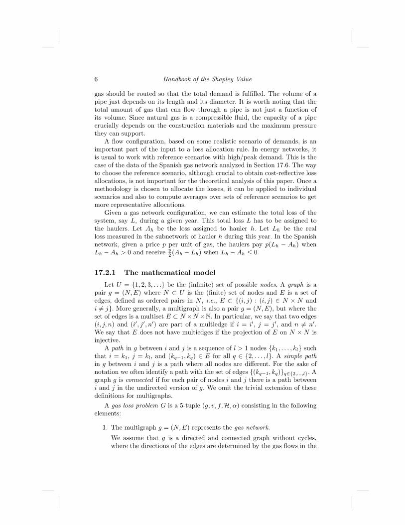
Example 1 Let G be the gas problem where

1. g = (N,E), where the set of nodes is N = {s1, s2, 1, c1, c2} and the setof edges is E = {(s1, 1), (1, c1), (s2, 1), (1, c2)}.

2. v(s1,1) = v(s2,1) = v(1,c1) = v(1,c2) = 100.

3. f(s1,1) = 20, f(s2,1) = 80, f(1,c1) = 60, and f(1,c2) = 40.

4. H = (H, {Eh}h∈H), where H = {h1, h2, h3} and Eh1 = {(s1, 1), (1, c1)},Eh2 = {(s2, 1)}, and Eh3 = {(1, c2)}.

5. α = 0.1.

This gas problem is represented in Figure 17.1 and will be used as a runningexample to illustrate some concepts and definitions. ♦

We now introduce some terminology. For each i ∈ N , we denote by Qi thegas balance at node i, i.e., the amount of gas leaving node i minus the amountof gas arriving at node i. Formally,

Qi =∑

(i,j)∈E

f(i,j) −∑

(j,i)∈E

f(j,i).

The set of suppliers S ⊂ N of the gas problem G is defined as the setof nodes s ∈ N such that Qs > 0. On the other hand, the set of consumers


s1

s2

1

c1

c2

f = 20

v = 100

f = 80

v = 100

f = 60

v = 100

f = 40

v = 100

h1

h2

h3

FIGURE 17.1: Representation of the gas problem in Example 1.

C ⊂ N is defined as the set of nodes c ∈ N such that Qc < 0. For the rest ofnodes i ∈ N \ (S ∪C), we have that Qi = 0. We make the natural assumptionthat total supply and total demand are balanced, namely,∑

s∈SQs = −

∑c∈C

Qc or, equivalently,∑i∈N

Qi = 0.

The total loss allowed to the haulers is L = α∑

s∈S Qs. The flow carried byeach hauler h ∈ H, denoted by fh, is defined as the gas that reaches one ofthe edges of hauler h from outside, that is, from some provider s ∈ S or froman edge of another hauler. Formally, we first define, for each node i ∈ N andeach hauler h ∈ H, Qh

i = max{∑

(i,j)∈Ehf(i,j)−

∑(j,i)∈Eh

f(j,i), 0}; if no edge

of hauler h contains node i we define Qhi = 0. Then, for each h ∈ H,

fh =∑i∈N

Qhi .

In particular, fh = 0 whenever Eh = ∅.1Given a gas problem G and a pair (s, c) ∈ S × C, we define P (s, c) as the

set of simple paths in g from s to c. We denote by P (S,C) the set of all simplepaths from suppliers to consumers. Namely,

P (S,C) =⋃

(s,c)∈S×C

P (s, c).

We now want to define an important notion for our analysis that we callhauler’s influence network, which, given a hauler h, would contain all edgeswhose gas might either reach some edge in Eh or come from some edge in Eh.Formally, for each h ∈ H, we define N h = (gh, vh, fh), as the subnetwork of

1There are alternative ways to define the notion of “flow carried by a hauler”, but, asfar as our analysis is concerned, they would lead to similar results. Our formulation is theone implicit in the Spanish Regulations ([3, 5]).


(g, v, f) where gh = (Nh, Eh) and

Eh = {e ∈ E : there is p ∈ P (S,C) with e ∈ p and p ∩ Eh 6= ∅},Nh = {i ∈ N : i ∈ e for some e ∈ Eh},vh = (ve)e∈Eh ,

fh = (fe)e∈Eh .

Sometimes we slightly abuse language and refer to an edge’s influence network,to mean the influence network that would have a hauler who owned only thatedge.

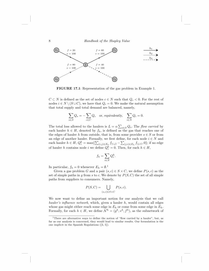
Example 1 (cont.) Going back to the gas problem in Figure 17.1, we havethat Qs1 = 20, Qs2 = 80, Q1 = 0, Qc1 = −60, and Qc2 = −40. Thus,S = {s1, s2} and C = {c1, c2}. The table below contains the different Qh

i flowbalances and Figure 17.2 represents the influence networks corresponding tothis example.

Qhi s1 s2 1 c1 c2 fhh1 20 0 40 0 0 60h2 0 80 0 0 0 80h3 0 0 40 0 0 40 ♦

Nh1

s1

s2

1

c1

c2

f = 20

v = 100

f = 80

v = 100

f = 60

v = 100

f = 40

v = 100

Nh2

s1

s2

1

c1

c2

f = 80

v = 100

f = 60

v = 100

f = 40

v = 100

Nh3

s1

s2

1

c1

c2

f = 20

v = 100

f = 80

v = 100

f = 40

v = 100

FIGURE 17.2: Illustration of the hauler’s influence networks of Example 1.

17.3 The Shapley rule

In [1] the authors study four rules that provide, for each gas loss problem,an allocation of the allowed loss among the different haulers. These rules,whose definitions can be seen in [1], are the following: the flow’s rule, Rflow,the aggregate edge’s rule, RAedge, the edge’s rule, Redge, and the proportionaltracing rule, RΓpt

.In this section we introduce a new allocation rule: the Shapley rule. In

order to do it we first associate, to each gas loss problem a cooperative game


with transferable utility, and then study the Shapley value of the associatedgame.

We start with some preliminaries on cooperative games. A cooperativegame with transferable utility, briefly a TU game, is a pair (H, l) where H isthe set of agents and, for each T ⊂ H, l(T ) denotes the amount that agentsin T can obtain by themselves. We assume that l(∅) = 0.

The Shapley value introduced in [14] is, by far, the most studied allocationrule in cooperative game theory. It associates, to each TU game (H, l) a vectorSh(H, l) ∈ RH such that, for each h ∈ H,

Shh(H, l) =∑

T⊂H\{h}

|T |! (|H| − |T | − 1)!

|H|!(l(T ∪ {h})− l(T )) .

In our context H represents the set of haulers and, for each T ⊂ H, l(T ),is the loss that haulers in T can have by “themselves”. Although there areseveral ways in which the l(T ) values can be defined, we present a naturalone inspired in the approach taken in [9] for flow games. In their model thereis also a set of agents who own the different edges of the network and thevalue of a group of agents T is defined as the maximum amount of flow thatcan be transported (from the source to the sink) using only edges belongingto agents in T . We apply the same principle to our model. Let fG(T ) denotethe maximum demand that can be satisfied using only edges of haulers inT , i.e., the maximum amount of gas that can be transported from suppli-ers to consumers without exceeding the capacities and demands of suppliersand consumers, respectively. We also assume that the capacity of an edgeis bounded by fe, the total amount of gas flowing through that edge in thegas problem under study. Then, we define lG(T ) = αfG(T ); in particular,lG(H) = αfG(H) = α

∑s∈S Qs = L. When no confusion arises we write l

instead of lG.The Shapley rule, RSh. For each gas problem G we define the Shapley

rule as RSh(G) = Sh(H, lG).Note that RSh(G) = αSh(H, fG).

Consider our running example. We first compute the associated cooper-ative game l. Hauler 1 can transport by himself 20 units. Since α = 0.1,lG (1) = 0.1 · 20 = 2. Haulers 1 and 2 can transport by themselves no morethan 60 units. They can do in several ways. For instance, 20 units through thepath {(s1, 1) , (1, c1)} and 40 units through the path {(s2, 1) , (1, c1)}. Sinceα = 0.1, lG (1, 2) = 0.1 · 60 = 6. Analogously we can obtain that

T {1} {2} {3} {1, 2} {1, 3} {2, 3} {1, 2, 3}lG (T ) 2 0 0 6 2 4 10

Thus the Shapley rule is RSh(G) = (4, 4, 2). In the table below we show, for


this example, the Shapley rule and the four rules defined in [1]:

h fh Rflow RAedge Redge RΓpt

RSh

1 60 3.33 5 4 4 42 80 4.44 3.33 4 4 43 40 2.22 1.66 2 2 2

Although in this example several rules lead to the same allocation, in generalthe five rules are all different from one another.

17.4 Properties

The main objective of this paper is to study the axiomatic behavior of theShapley rule, and compare this behavior with that of the other rules stud-ied in [1]. In order to do so, we focus our analysis in precisely the propertiesintroduced in that paper, and refer the reader to the discussions therein foradditional insights. Since these properties are inspired in the principles men-tioned in different regulations and directives of the European Union regulation,the authors in [1] present the following discussion to provide some additionalmotivation to the properties and their underlying principles:

In Directive 2003/55/EC of the European parliament andthe council of 26 June 2003 ([13]), concerning common rulesfor the internal market in natural gas, establishes some gen-eral principles that must be pursued. Some of them are thefollowing:

1. “tariffs are published prior to their entry into force”.

2. “the provision of adequate economic incentives, using, whereappropriate, all existing national and Community tools. These toolsmay include liability mechanisms to guarantee the necessary invest-ment”.

3. “national regulatory authorities should ensure that transmission anddistribution tariffs are non-discriminatory and cost-reflective”.

4. “Progressive opening of markets towards full competition shouldas soon as possible remove differences between Member States.”

The Spanish regulation ensures that tariffs are publishedprior to their entry into force. Moreover, since the amount


received or paid by each hauler depends monotonically ontheir loss (the larger is the loss, the larger is the amountthe hauler pays) we can argue that it provides the adequateeconomic incentives.Regarding the principles of being non-discriminatory, cost-reflective, and foster competition. We introduce some prop-erties related to these principles.”

17.4.1 Cost reflective properties

The first property requires that haulers that do not transport gas do nothave any assigned loss and the second one says that if two gas problems onlydiffer on edges without flow, then the losses assigned to each hauler shouldcoincide.

Null hauler (NH). Let G = (g, v, f,H, α) and h ∈ H be such that, foreach e ∈ Eh, fe = 0. Then, Rh(G) = 0.

Independence of unused edges (IUE). Let the gas problems G =(g, v, f,H, α) and G = (g, v, f , H, α) be such that H = H and, for each h ∈ H,Eh = Eh \ E, where E ⊂ E satisfies that, for each e ∈ E \ E, fe = fe andve = ve, and, for each e ∈ E, fe = 0. Then, R(G) = R(G).

A cost-reflective rule should not be sensitive to “equivalent” representa-tions of the same network. The next two properties try to capture this idea.

Independence of edge sectioning (IES). Let the gas problems G =

(g, v, f,H, α) and G = (g, v, f , H, α) be such that H = H and there are h ∈ Hand (i, j) ∈ Eh satisfying

• g = (N , E), where N = N ∪ {l} and l /∈ N , Eh = (Eh\{(i, j)}) ∪{(i, l), (l, j)} and, for each h ∈ H\{h}, Eh = Eh, and

• f(i,l) = f(l,j) = f(i,j), v(i,l) + v(l,j) = v(i,j), and, for each e ∈ E\{(i, j)},fe = fe and ve = ve.

2

Then, for each h ∈ H, Rh(G) = Rh(G).Independence of edge multiplication (IEM). Let G = (g, v, f,H, α)

and G = (g, v, f , H, α) be such that H = H and there are h ∈ H, e =(i, j,m) ∈ E, e1 = (i, j, l1) ∈ E, and e2 = (i, j, l2) ∈ E satisfying

• g = (N, E), where Eh = (Eh \ {e}) ∪ {e1, e2} and, for each h ∈ H\{h},Eh = Eh, and

2The condition v(i,l) + v(l,j) = v(i,j) just reflects that, when a pipe is transversely cut(orthogonally to the direction of the flow), the volume of the resulting two pipes adds upto the volume of the original pipe (and the same flow that was crossing the original pipe iscrossing the two pipes in which it has been divided f(i,l) = f(l,j) = f(i,j)).


• fe = fe1 + fe2 , ve = ve1 = ve2 , and, for each e ∈ E\{e}, fe = fe andve = ve.

3

Then, for each h ∈ H, Rh(G) = Rh(G).To prevent haulers from artificially distorting the final allocation of losses,

if two haulers engage in some trades affecting their own edges, then the restof the haulers should not be affected. This implies, in particular, that the lossallocated to a hauler does not depend on who owns the edges different fromhis own.

Independence by sales (IS). Let G = (g, v, f,H, α), G = (g, v, f, H, α),h1 and h2 in H, and e ∈ E be such that Eh1

= Eh1\{e}, Eh2

= Eh2∪ {e},

and, for each h ∈ H\{h1, h2}, Eh = Eh. Then, for each h ∈ H\{h1, h2},Rh(G) = Rh(G).4

Independence of irrelevant changes (IIC). Consider the gas problemsG = (g, v, f,H, α) and G = (g, v, f , H, α) and let h ∈ H ∩ H be such thatN h = N h. Then, Rh(G) = Rh(G).

17.4.2 Non-discriminatory properties

The most standard non-discriminatory principle says that we should offeran equal treatment to equal agents. Some of the following properties deal withformalizations of this general notion.

Symmetry on edges (SE). Let G = (g, v, f,H, α) and h, h ∈ H be suchthat Eh = {e}, Eh = {e}, fe = fe, and ve = ve. Then, Rh(G) = Rh(G).

Symmetry on paths (SP). Let G = (g, v, f,H, α) and h, h ∈ H be suchthat Eh = {e}, Eh = {e}, ve = ve, and N h = N h. Then, Rh(G) = Rh(G).

The following properties build upon the idea that there should be somekind of proportionality on flow and volume.

Flow proportionality on edges (FPE). Let G = (g, v, f,H, α) andh, h ∈ H be such that Eh = {e}, Eh = {e}, and ve = ve. Then, if fe > 0, wehave

Rh(G) =fefeRh(G).

Volume proportionality on edges (VPE). Let G = (g, v, f,H, α) andh, h ∈ H be such that Eh = {e}, Eh = {e}, and fe = fe. Then,

Rh(G) =veveRh(G).

3In this case, the condition ve = ve1 = ve2 just reflects that the original pipe e is beingreplaced by two pipes identical to it: same volume and same endpoints. The total flow inthe network remains unchanged, so these two new pipes, together, carry the same flow as e(fe = fe1 + fe2 ).

4The rules satisfying IS have an interesting property, which in [1] is referred to as edgedecomposability. Namely, these rules can be computed in a two stage procedure. We firstdecide the allowed loss on each edge and later compute the allowed loss to each hauleradding the amount assigned to each of his edges.


Volume proportionality on paths (VPP). Let G = (g, v, f,H, α) andh, h ∈ H be such that Eh = {e}, Eh = {e}, and N h = N h. Then,

Rh(G) =veveRh(G).

17.4.3 Properties to foster competition

The way in which losses are allocated among haulers should not harmcompetition among agents. In particular, two haulers should not be better offby merging together.

Merging proofness (MP). Let G = (g, v, f,H, α), G = (g, v, f, H, α),

h1, h2 ∈ H, and h ∈ H be such that Eh = Eh1∪ Eh2

and, for each h ∈H \ {h1, h2}, Eh = Eh . Then Rh(G) ≤ Rh1

(G) +Rh2(G).

17.5 Axiomatic behavior of the Shapley rule

We present now the main result of this paper, which shows what propertiesare satisfied by the the Shapley rule.

Proposition 1 1. The Shapley rule satisfies NH, IUE, IES, IEM, and SP.

2. The Shapley rule does not satisfy IS, SE, FPE, VPE, VPP, IIF, IIC,and MP.

Proof 1 We start by proving statement 1.• NH. Let G = (g, v, f,H, α) and h ∈ H be such that, for each e ∈ Eh fe =

0. Since the edges of hauler h do not carry flow, they never help to increasethe total flow that can be carried between a supplier and a consumer. Thus,for each T ⊂ H\{h}, we have that lG(T ) = lG(T ∪ {h}) and the definition ofthe Shapley value implies that RSh

h = 0.• IUE. Let G = (g, v, f,H, α) and G = (g, v, f , H, α) be as in the definition

of IUE, that is, there is E ⊂ E such that, for each h ∈ H, Eh = Eh \ E and,for each e ∈ E, fe = 0.

Let T ⊂ H be a set of players. Again, the edges that do not carry flownever help to increase the total flow that can be carried between a supplierand a consumer. Thus, they can be removed for the computation of the TUgame associated with G and, therefore, for each T ⊂ H, lG(T ) = lG(T ). Thus,RSh(G) = RSh(G).• IES. Let G = (g, v, f,H, α) and G = (g, v, f , H, α) be two problems that

only differ because there are h ∈ H and (i, j) ∈ Eh satisfying that (i, j) issectioned in two consecutive edges (i, l), (l, j) ∈ Eh.


Since f(i,j) = f(i,l) = f(l,j), edge sectioning does not change the maximumflow that can be carried from consumers to suppliers. Then, for each T ⊂ H,lG(T ) = lG(T ) and, therefore, for each h ∈ H, RSh

h (G) = RShh (G).

• IEM. Let G = (g, v, f,H, α) and G = (g, v, f ,H, α) be two problems that

only differ because there are h ∈ H and e ∈ Eh satisfying that e is duplicatedin two multiedges e1, e2 ∈ Eh, with ve = ve1 = ve2 .

Since fe = fe1 +fe2 , edge multiplication does not change the maximum flowthat can be carried from consumers to suppliers because we only have to splitamong fe1 and fe2 the maximum flow that went through fe. Then, for eachT ⊂ H, lG(T ) = lG(T ) and, therefore, for each h ∈ H, RSh

h (G) = RShh (G).

• SP. Let G = (g, v, f,H, α) and h, h ∈ H be such that Eh = {e}, Eh ={e}, ve = ve and N h = N h.

Since N h = N h we have that fe = fe and, for each p ∈ P (S,C), e ∈ p ifand only if e ∈ p. Then, for each T ⊂ H\{h, h} we have lG(T ∪h) = lG(T ∪h).Thus, the definition of the Shapley value implies that RSh

h (G) = RShh

(G).

Next, we present some counterexamples to prove statement 2.• IS. Since IS is stronger than MP (Proposition 1 in [1]) and RSh does

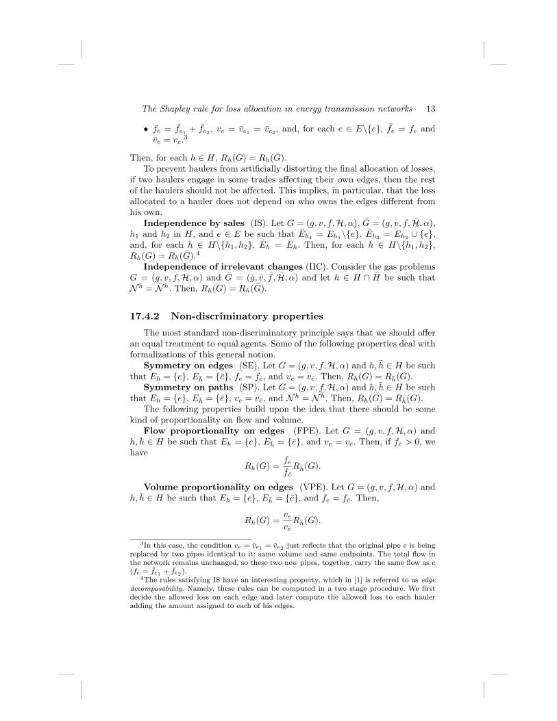
not satisfy MP (see below), RSh does not satisfy IS.• SE. Let G = (g, v, f,H, α) be as in the picture below.

G2

1

1

2

h1

h2

h3

Problem G is as in the definition of SE, since h1 = {e1} and h3 = {e2} withfe1 = fe2 = 2 and ve1 = ve2 . However, h3 can satisfy some demand on hisown, while h1 needs h2. In particular, we get RSh

h1(G) = α 6= 2α = RSh

h3(G).

• FPE and VPE. Since FPE and VPE are stronger than SE (Proposition 1in [1]) and RSh does not satisfy SE, RSh satisfies neither FPE nor VPE.• VPP. Let G = (g, v, f,H, α), h1 and h2 as in the picture below.

Gf = 1v = 1

f = 1v = 2

h1

h2

Clearly, RShh2

(G) = RShh1

(G) 6= 2RShh1

(G) =vh2

vh1RSh

h1(G).

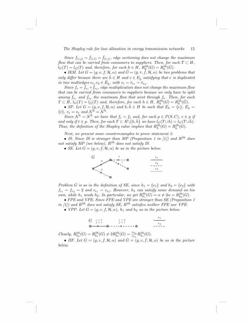
• IIF. Let G = (g, v, f,H, α) and G = (g, v, f ,H, α) be as in the picturebelow.


G

1

3 7 1

5 1

7

G

1

3 7 11

5 11

7

h1

h2

h3

Problems G and G are as in the definition of IIF. Note that there are twoedges where the flow increases and N h1 = N h1 . In this case we get the games

– lG({h1}) = 0, lG({h2}) = α, lG({h3}) = α, lG({h1, h2}) = 2α,lG({h1, h3}) = 2α, lG({h2, h3}) = 8α, lG({h1, h2, h3}) = 9α and

– lG({h1}) = 0, lG({h2}) = 3α, lG({h3}) = 7, lG({h1, h2}) = 3α,lG({h1, h3}) = 8α, lG({h2, h3}) = 18α, lG({h1, h2, h3}) = 19α.

The corresponding Shapley values are so that

RShh1

(G) = α4

66= α

3

6= RSh

h1(G).

The key is that the marginal contribution of hauler h1 to hauler h2 changesfrom G to G.• IIC. Since IIC is stronger than IIF (Proposition 1 in [1]) and RSh does

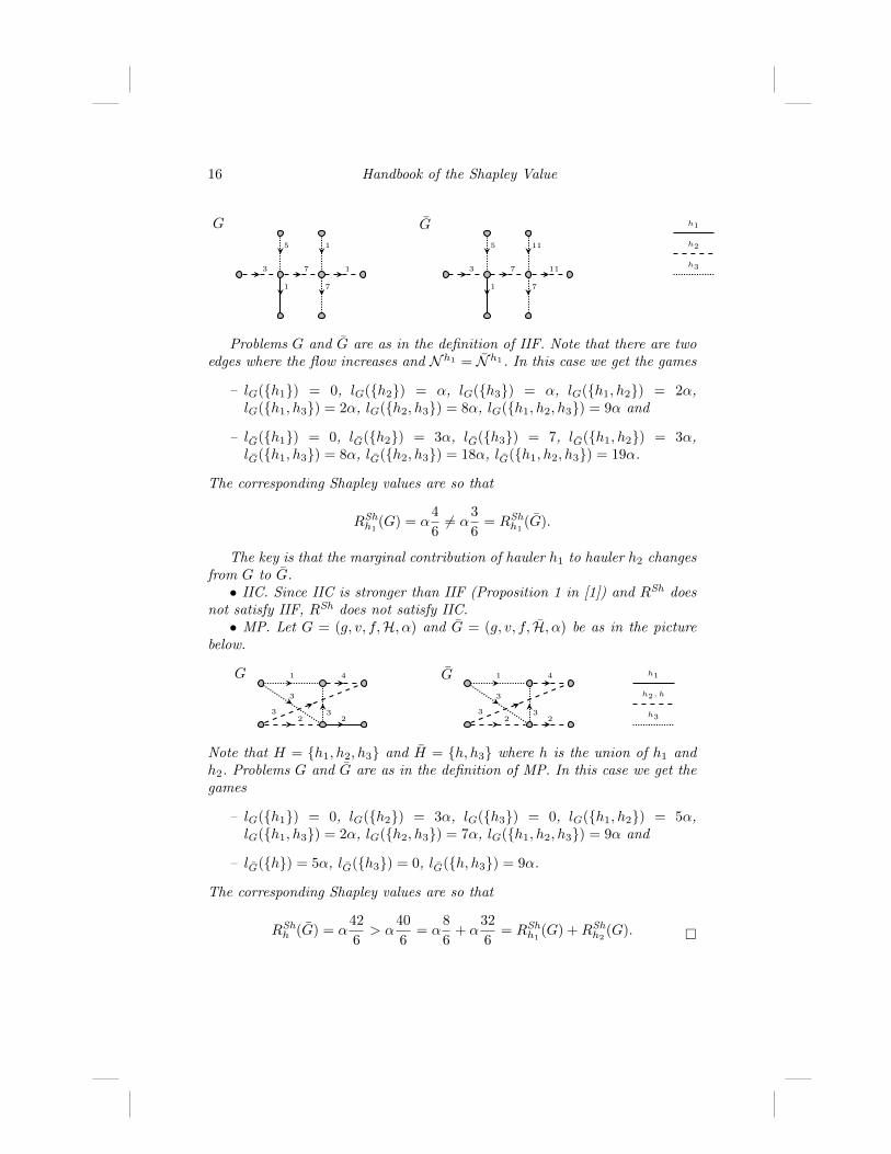
not satisfy IIF, RSh does not satisfy IIC.• MP. Let G = (g, v, f,H, α) and G = (g, v, f, H, α) be as in the picture

below.

G

223

41

3

3

G

223

41

3

3

h1

h2, h

h3

Note that H = {h1, h2, h3} and H = {h, h3} where h is the union of h1 andh2. Problems G and G are as in the definition of MP. In this case we get thegames

– lG({h1}) = 0, lG({h2}) = 3α, lG({h3}) = 0, lG({h1, h2}) = 5α,lG({h1, h3}) = 2α, lG({h2, h3}) = 7α, lG({h1, h2, h3}) = 9α and

– lG({h}) = 5α, lG({h3}) = 0, lG({h, h3}) = 9α.

The corresponding Shapley values are so that

RShh (G) = α

42

6> α

40

6= α

8

6+ α

32

6= RSh

h1(G) +RSh

h2(G). �


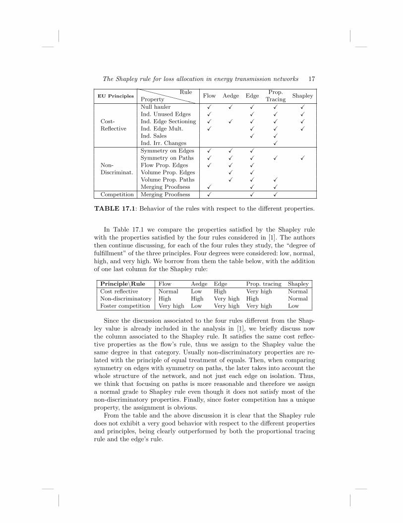
EU Principles

XXXXXXXXXPropertyRule

Flow Aedge EdgeProp.

TracingShapley

Null hauler X X X X XInd. Unused Edges X X X X

Cost- Ind. Edge Sectioning X X X X XReflective Ind. Edge Mult. X X X X

Ind. Sales X XInd. Irr. Changes XSymmetry on Edges X X XSymmetry on Paths X X X X X

Non- Flow Prop. Edges X X XDiscriminat. Volume Prop. Edges X X

Volume Prop. Paths X X XMerging Proofness X X X

Competition Merging Proofness X X X

TABLE 17.1: Behavior of the rules with respect to the different properties.

In Table 17.1 we compare the properties satisfied by the Shapley rulewith the properties satisfied by the four rules considered in [1]. The authorsthen continue discussing, for each of the four rules they study, the “degree offulfillment” of the three principles. Four degrees were considered: low, normal,high, and very high. We borrow from them the table below, with the additionof one last column for the Shapley rule:

Principle\Rule Flow Aedge Edge Prop. tracing Shapley

Cost reflective Normal Low High Very high NormalNon-discriminatory High High Very high High NormalFoster competition Very high Low Very high Very high Low

Since the discussion associated to the four rules different from the Shap-ley value is already included in the analysis in [1], we briefly discuss nowthe column associated to the Shapley rule. It satisfies the same cost reflec-tive properties as the flow’s rule, thus we assign to the Shapley value thesame degree in that category. Usually non-discriminatory properties are re-lated with the principle of equal treatment of equals. Then, when comparingsymmetry on edges with symmetry on paths, the later takes into account thewhole structure of the network, and not just each edge on isolation. Thus,we think that focusing on paths is more reasonable and therefore we assigna normal grade to Shapley rule even though it does not satisfy most of thenon-discriminatory properties. Finally, since foster competition has a uniqueproperty, the assignment is obvious.

From the table and the above discussion it is clear that the Shapley ruledoes not exhibit a very good behavior with respect to the different propertiesand principles, being clearly outperformed by both the proportional tracingrule and the edge’s rule.


There are many problems where the Shapley value of an associated coop-erative game has many interesting properties compared with other rules inthe same setting. We can mention, for instance, airport problems (see [11]),queuing problems (see [12] and [7], and minimum cost spanning tree problems(see [10] and [2]). Nevertheless in our case the Shapley value satisfies less prop-erties than other rules. Of course it could be possible that, if we define theassociated cooperative game lG in a different way, we could obtain a Shapleyvalue with more properties.

In the next section we take a different approach to assess the performanceof the Shapley rule, which can be seen as complementary to the one developedin this section. More precisely, we study the allocations the Shapley rule pro-poses in different problems, a case study with real data and a set of variationsof it, and comparing these allocations with the ones proposed by the otherfour rules.

17.6 Application to the Spanish gas transmission net-work

17.6.1 Case study with real data

In this section we apply the Shapley rule to the Spanish gas transmissionnetwork. We compare the allocation proposed by the Shapley rule with theallocations proposed by the four rules considered in [1]. We build upon theanalysis there, and take as benchmark scenario one in which demands fol-low from reported figures for a hypothetical day of very high demand in theSpanish gas network.5

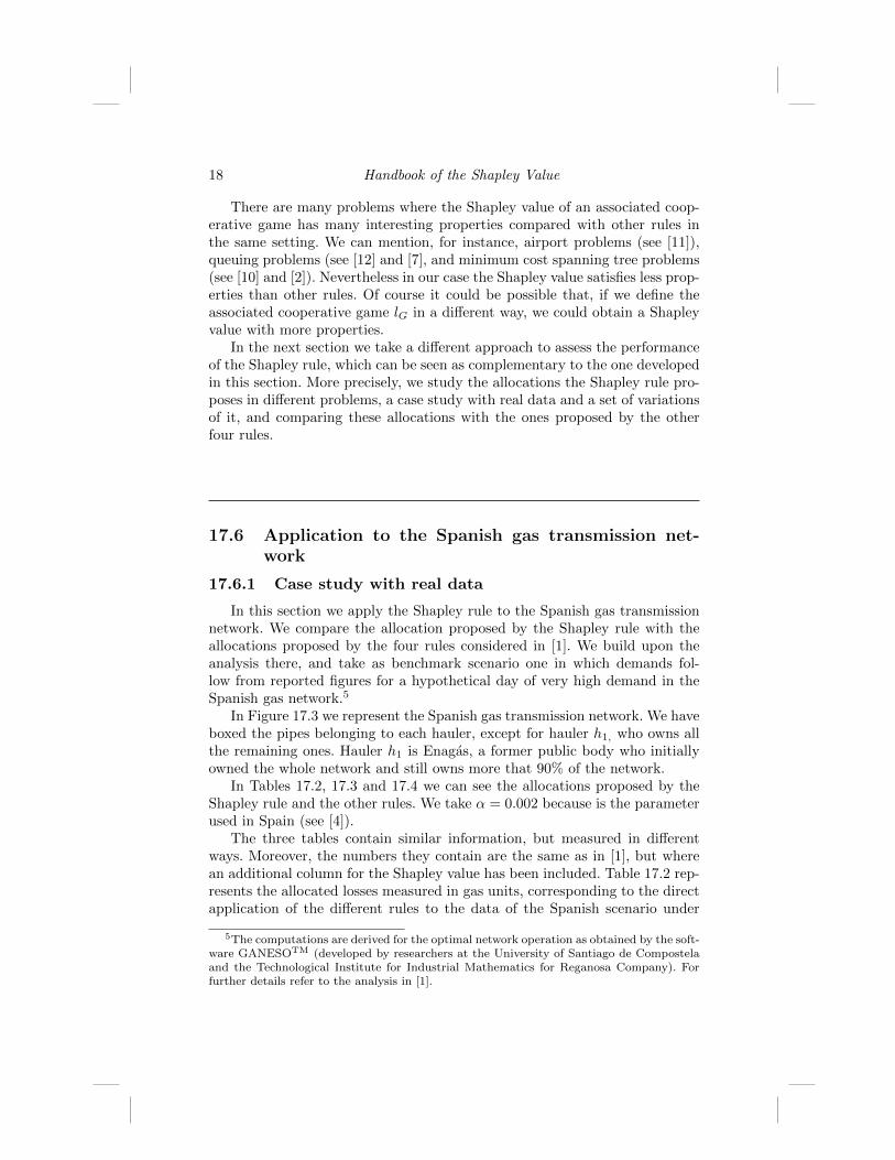
In Figure 17.3 we represent the Spanish gas transmission network. We haveboxed the pipes belonging to each hauler, except for hauler h1, who owns allthe remaining ones. Hauler h1 is Enagas, a former public body who initiallyowned the whole network and still owns more that 90% of the network.

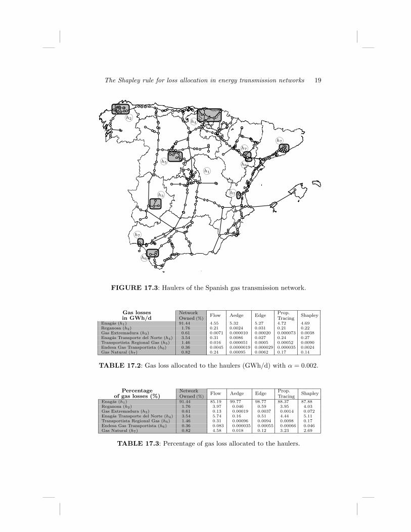
In Tables 17.2, 17.3 and 17.4 we can see the allocations proposed by theShapley rule and the other rules. We take α = 0.002 because is the parameterused in Spain (see [4]).

The three tables contain similar information, but measured in differentways. Moreover, the numbers they contain are the same as in [1], but wherean additional column for the Shapley value has been included. Table 17.2 rep-resents the allocated losses measured in gas units, corresponding to the directapplication of the different rules to the data of the Spanish scenario under

5The computations are derived for the optimal network operation as obtained by the soft-ware GANESOTM (developed by researchers at the University of Santiago de Compostelaand the Technological Institute for Industrial Mathematics for Reganosa Company). Forfurther details refer to the analysis in [1].


h1

h2

h3

h4

h5 h6

h6

h7

h7

h7

h7

FIGURE 17.3: Haulers of the Spanish gas transmission network.

Gas losses NetworkFlow Aedge Edge

Prop.Shapley

in GWh/d Owned (%) TracingEnagas (h1) 91.44 4.55 5.32 5.27 4.72 4.69Reganosa (h2) 1.76 0.21 0.0024 0.031 0.21 0.22Gas Extremadura (h3) 0.61 0.0071 0.000010 0.00020 0.000073 0.0038Enagas Transporte del Norte (h4) 3.54 0.31 0.0086 0.027 0.24 0.27Transportista Regional Gas (h5) 1.46 0.016 0.000051 0.0005 0.00052 0.0090Endesa Gas Transportista (h6) 0.36 0.0045 0.0000019 0.000029 0.000035 0.0024Gas Natural (h7) 0.82 0.24 0.00095 0.0062 0.17 0.14

TABLE 17.2: Gas loss allocated to the haulers (GWh/d) with α = 0.002.

Percentage NetworkFlow Aedge Edge

Prop.Shapley

of gas losses (%) Owned (%) TracingEnagas (h1) 91.44 85.19 99.77 98.77 88.37 87.88Reganosa (h2) 1.76 3.97 0.046 0.59 3.95 4.03Gas Extremadura (h3) 0.61 0.13 0.00019 0.0037 0.0014 0.072Enagas Transporte del Norte (h4) 3.54 5.74 0.16 0.51 4.44 5.11Transportista Regional Gas (h5) 1.46 0.31 0.00096 0.0094 0.0098 0.17Endesa Gas Transportista (h6) 0.36 0.083 0.000035 0.00055 0.00066 0.046Gas Natural (h7) 0.82 4.58 0.018 0.12 3.23 2.69

TABLE 17.3: Percentage of gas loss allocated to the haulers.


Monetary equivalent NetworkFlow Aedge Edge

Prop.Shapleyin millions of e Owned (%) Tracing

Enagas (h1) 91.44 49.77 58.30 57.71 51.64 51.35Reganosa (h2) 1.76 2.32 0.027 0.34 2.31 2.36Gas Extremadura (h3) 0.61 0.077 0.00011 0.0022 0.00080 0.042Enagas Transporte del Norte (h4) 3.54 3.35 0.095 0.30 2.60 2.99Transportista Regional Gas (h5) 1.46 0.18 0.00056 0.0055 0.0057 0.098Endesa Gas Transportista (h6) 0.36 0.049 0.000020 0.00032 0.00039 0.027Gas Natural (h7) 0.82 2.68 0.010 0.068 1.89 1.57

TABLE 17.4: Annual monetary equivalent, assuming 1 GWh/d = 30000 e.

consideration. Table 17.3 represents the percentage allocated to each hauler.Finally, Table 17.4 represents the estimation of the annual monetary equiva-lent, provided that the same demands repeat each and every day. Since thescenario under consideration comes from a peak day, whose demand is aroundtwice the demand of an average day, one would get more realistic estimationsafter dividing by two the amounts in Table 17.4. In practice one might applythe chosen rule on a daily basis and then add up the daily allocations to getthe annual loss allocation.

The aggregate edge’s rule assign 99.77% of the allocated losses to Enagas,which we believe is unfair. As it was argued in [1] the aggregate edge’s rulesize discriminates, penalizing small haulers and favoring mergers, which hurtscompetition. This probably explains why most Spanish haulers strongly op-posed to the aggregate edges rule until it was finally replaced by the flow’srule.

In this case we can see that the allocation proposed by the Shapley ruleis quite similar to the one proposed by the proportional tracing rule. In thenext section we further explore this connection.

17.6.2 Simulation study building upon the real data

Given the results in the analysis above, it is natural to wonder whether ornot the similarity between the allocations proposed by the Shapley rule andthe proportional tracing rule is just a coincidence for the given data. In order toget additional evidence, we have run a simulation study based on the originalscenario, but where relevant data of the problem are randomly modified. Moreprecisely, we have generated 10000 scenarios from the benchmark using thefollowing procedure:

• The only information that is modified from scenario to scenario is theownership relation between edges and haulers, with pipes being ran-domly assigned to haulers.

• In order to get reasonably connected networks, the random assignmentis not performed on individual pipes, but on some predetermined groupsof pipes. More precisely, the pipes are divided in 16 groups, correspond-ing to the 16 Spanish autonomous communities (setting aside CanaryIslands, which contain no pipes of the high-presure network).


• Then, each of the 16 groups is randomly assigned to one of the 7 availablehaulers. We keep the same number of haulers of the Spanish networkwhich should provide enough richness to the random generating pro-cess (note that a hauler might end up with no assigned pipes in somerealizations).

• This random process is repeated 10000 times, with the goal of obtain-ing very diverse realizations: homogeneous haulers, a single dominanthauler, split between medium haulers and small ones,. . .

• For each realization we obtain the resulting loss allocation for the fiverules discussed in this paper. Finally, we compute the matrix of correla-tions between the allocations proposed by these five rules and also withthe vector of the length of pipes owned by each hauler.6

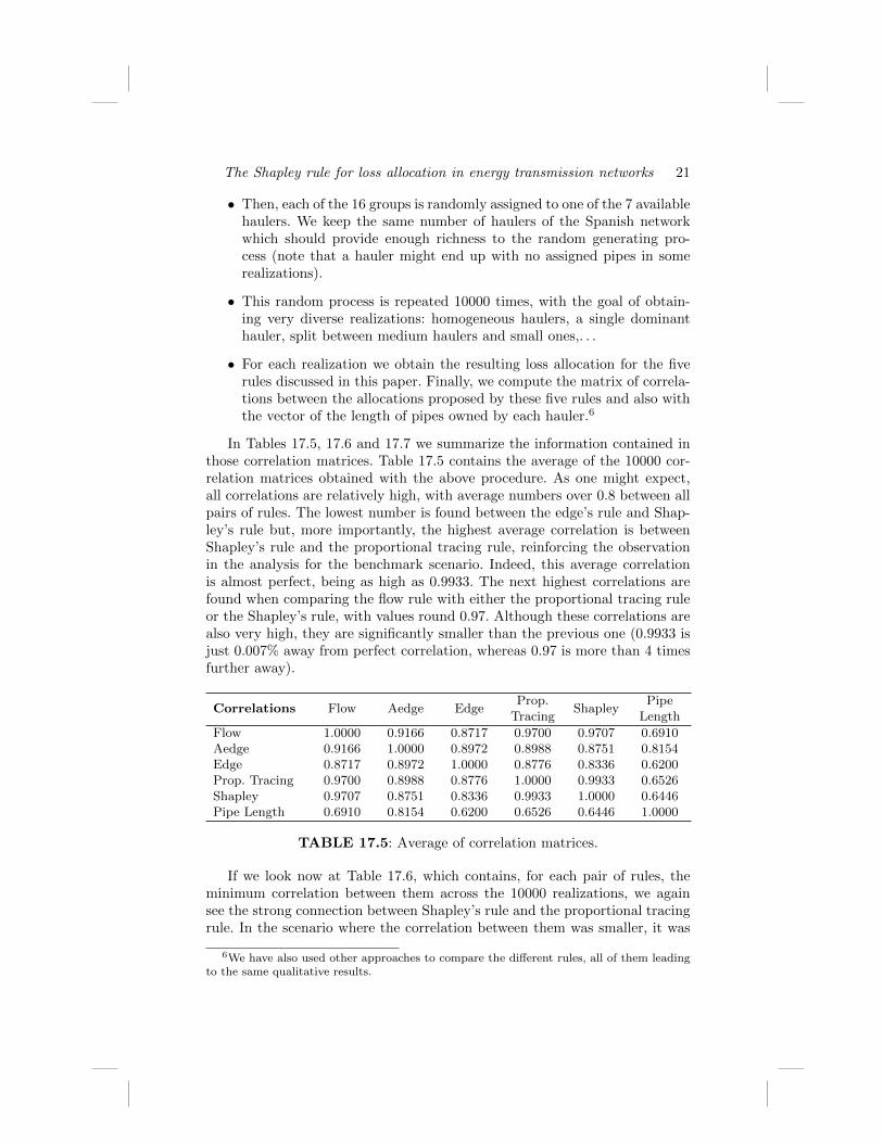
In Tables 17.5, 17.6 and 17.7 we summarize the information contained inthose correlation matrices. Table 17.5 contains the average of the 10000 cor-relation matrices obtained with the above procedure. As one might expect,all correlations are relatively high, with average numbers over 0.8 between allpairs of rules. The lowest number is found between the edge’s rule and Shap-ley’s rule but, more importantly, the highest average correlation is betweenShapley’s rule and the proportional tracing rule, reinforcing the observationin the analysis for the benchmark scenario. Indeed, this average correlationis almost perfect, being as high as 0.9933. The next highest correlations arefound when comparing the flow rule with either the proportional tracing ruleor the Shapley’s rule, with values round 0.97. Although these correlations arealso very high, they are significantly smaller than the previous one (0.9933 isjust 0.007% away from perfect correlation, whereas 0.97 is more than 4 timesfurther away).

Correlations Flow Aedge EdgeProp.

TracingShapley

PipeLength

Flow 1.0000 0.9166 0.8717 0.9700 0.9707 0.6910Aedge 0.9166 1.0000 0.8972 0.8988 0.8751 0.8154Edge 0.8717 0.8972 1.0000 0.8776 0.8336 0.6200Prop. Tracing 0.9700 0.8988 0.8776 1.0000 0.9933 0.6526Shapley 0.9707 0.8751 0.8336 0.9933 1.0000 0.6446Pipe Length 0.6910 0.8154 0.6200 0.6526 0.6446 1.0000

TABLE 17.5: Average of correlation matrices.

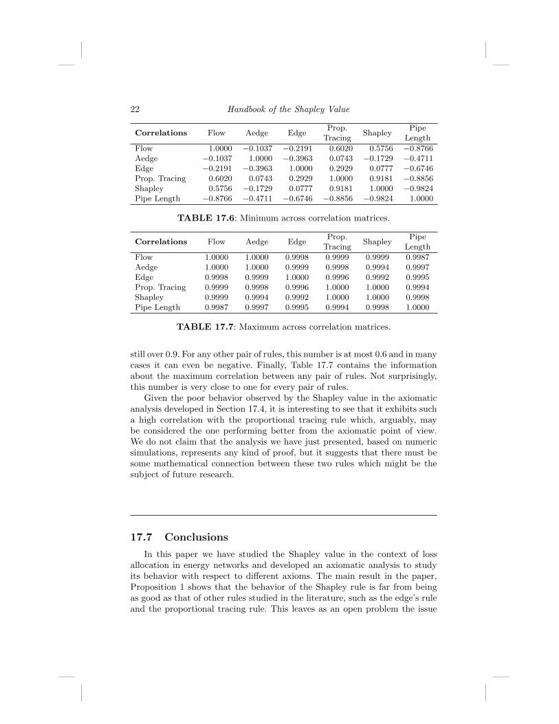
If we look now at Table 17.6, which contains, for each pair of rules, theminimum correlation between them across the 10000 realizations, we againsee the strong connection between Shapley’s rule and the proportional tracingrule. In the scenario where the correlation between them was smaller, it was

6We have also used other approaches to compare the different rules, all of them leadingto the same qualitative results.



TracingShapley

PipeLength

Flow 1.0000 −0.1037 −0.2191 0.6020 0.5756 −0.8766Aedge −0.1037 1.0000 −0.3963 0.0743 −0.1729 −0.4711Edge −0.2191 −0.3963 1.0000 0.2929 0.0777 −0.6746Prop. Tracing 0.6020 0.0743 0.2929 1.0000 0.9181 −0.8856Shapley 0.5756 −0.1729 0.0777 0.9181 1.0000 −0.9824Pipe Length −0.8766 −0.4711 −0.6746 −0.8856 −0.9824 1.0000

TABLE 17.6: Minimum across correlation matrices.


TracingShapley

PipeLength

Flow 1.0000 1.0000 0.9998 0.9999 0.9999 0.9987Aedge 1.0000 1.0000 0.9999 0.9998 0.9994 0.9997Edge 0.9998 0.9999 1.0000 0.9996 0.9992 0.9995Prop. Tracing 0.9999 0.9998 0.9996 1.0000 1.0000 0.9994Shapley 0.9999 0.9994 0.9992 1.0000 1.0000 0.9998Pipe Length 0.9987 0.9997 0.9995 0.9994 0.9998 1.0000

TABLE 17.7: Maximum across correlation matrices.

still over 0.9. For any other pair of rules, this number is at most 0.6 and in manycases it can even be negative. Finally, Table 17.7 contains the informationabout the maximum correlation between any pair of rules. Not surprisingly,this number is very close to one for every pair of rules.

Given the poor behavior observed by the Shapley value in the axiomaticanalysis developed in Section 17.4, it is interesting to see that it exhibits sucha high correlation with the proportional tracing rule which, arguably, maybe considered the one performing better from the axiomatic point of view.We do not claim that the analysis we have just presented, based on numericsimulations, represents any kind of proof, but it suggests that there must besome mathematical connection between these two rules which might be thesubject of future research.

17.7 Conclusions

In this paper we have studied the Shapley value in the context of lossallocation in energy networks and developed an axiomatic analysis to studyits behavior with respect to different axioms. The main result in the paper,Proposition 1 shows that the behavior of the Shapley rule is far from beingas good as that of other rules studied in the literature, such as the edge’s ruleand the proportional tracing rule. This leaves as an open problem the issue


of finding new desirable properties that the Shapley rule might satisfy andwhich might ultimately lead to an axiomatic characterization.

Interestingly, we then develop a comparative analysis of the different allo-cation rules on a set of problems originated from real data and observe thatthe Shapley rule has a very high correlation (over 0.99) with the proportionaltracing rule. This may seem a bit contradictory with the fact that these tworules exhibit a very different behavior with respect to the set of axioms dis-cussed in Section 17.4. Then, an open question for future research would beto understand the mechanism driving this unusually high correlation.

Acknowledgements

The authors acknowledge support from Ministerio de Economıa y Com-petitividad and FEDER through projects MTM2014-60191-JIN, ECO2014-52616-R, and ECO2015-70119-REDT and from Xunta de Galicia throughprojects INCITE09-207-064-PR, GRC 2015/014 and ED431C 2017/38. Gus-tavo Bergantinos acknowledges support from Fundacion Seneca de la Regionde Murcia through project 19320/PI/14. Angel M. Gonzalez-Rueda acknowl-edges support from Ministerio de Educacion through Grant FPU13/01130.

Bibliography

[1] G. Bergantinos, J. Gonzalez Dıaz, A. M. Gonzalez-Rueda, andM. P. Fernandez de Cordoba. Loss allocation in energy transmissionnetworks. Games and Economic Behavior, 102:69–97, 2017.

[2] G. Bergantinos and J. Vidal-Puga. A fair rule in minimum cost spanningtree problems. Journal of Economic Theory, 137:326–352, 2007.

[3] Boletın Oficial del Estado. Incentivo a la reduccion de mermas en la red detransporte. In Orden ITC/3128/2011, volume 278. Spanish Government,2011.

[4] Boletın Oficial del Estado. Coeficientes de mermas en las instalacionesgasistas. In Orden IET/2446/2013, volume 312. Spanish Government,December 2013.

[5] Boletın Oficial del Estado. Incentivo a la reduccion de mermas en lared de transporte (amendment). In Orden IET/2446/2013, volume 312.Spanish Government, December 2013.

[6] British Petroleum. Bp statistical review of world energy. Annual report,2013.

[7] Y. Chun. A pessimistic approach to the queueing problem. MathematicalSocial Sciences, 51:171–181, 2006.

[8] Enerdata. Global energy statistical yearkbook. Annual report, 2017.

[9] E. Kalai and E. Zemel. Totally balanced games and games of flow. Math-ematics of Operations Research, 7:476–478, 1982.

[10] A. Kar. Axiomatization of the Shapley value on minimum cost spanningtree games. Games and Economic Behavior, 38:265–277, 2002.

[11] S. C. Littlechild and G. Owen. A simple expression for the Shapley valuein a special case. Management Science, 20:370–372, 1973.

[12] F. Maniquet. A characterization of the Shapley value in queueing prob-lems. Journal of Economic Theory, 109:90–103, 2003.

25

26 Bibliography

[13] Regulation (EC). Common rules for the internal market in natural gasand repealing directive 98/30/ec. Official Journal of the European Union(Legislation Series), 176:57–77, no. 55/2003.

[14] L. S. Shapley. A value for n-person games. In H. Kuhn and A. Tucker,editors, Contributions to the theory of games II, volume 28 of Annals ofMathematics Studies. Princeton University Press, Princeton, 1953.

Documents

Handbook of the Shapley Value