Hamiltonians for Quantum Computing

Vladimir Privmana, Dima Mozyrskya, and Steven P. Hotalingb

aDepartment of Physics, Clarkson University, Potsdam, New York 13699-5820

bAir Force Materiel Command, Rome Laboratory/Photonics Division25 Electronic Parkway, Rome, New York 13441-4515

ABSTRACT

We argue that the analog nature of quantum computing makes the usual design approach of constructing complicatedlogical operations from many simple gates inappropriate. Instead, we propose to design multi-spin quantum gatesin which the input and output two-state systems (spins) are not necessarily identical. We outline the design criteriafor such devices and then review recent results for single-unit Hamiltonians that accomplish the NOT and XORfunctions.

Keywords: Quantum computing, Analog computing, Hamiltonians for quantum gates

1. INTRODUCTION

One of the great challenges of the physics of nanoscale systems has been the design of atomic-size devices oper-ating in a quantum-coherent fashion. Dimensions of semiconductor computer components will soon reach1 about0.25µm = 2500 A, which is well above the atomic sizes at which quantum-mechanical effects are important. How-ever, it is generally expected that as the miniaturization continues, atomic dimensions will be reached. This articleconcerns with quantum computing, i.e., nanoscale devices that perform logical operations while maintaining quan-tum coherence. Some early studies2–4,8,9 considered how quantum mechanics affects the foundations of computerscience; issues such as limitations on classical computation due to quantum fluctuations, etc., have been raised. Amore recent development4–32 has been to utilize the quantum nature of components of atomic dimensions for moreefficient computations involving quantum-coherent evolution.

Quantum computing has attracted a lot of interest recently owing to several new features. Firstly, it maybe faster than classical computing: new fast quantum algorithms have been proposed.33–37 Error correction tech-niques,10,27,33,38–42 unitary operations corresponding to the simplest logic gates,5–32 and some Hamiltonians for gateoperation10,11,14,24,28–32,43 have been explored. Ideas on how to combine the simplest quantum gates have been putforth.7,15,44 Experimentally, there are several atomic-scale systems where the simplest quantum-gate functions havebeen recently realized26,45,46 or contemplated.19

There remain, however, many conceptual difficulties with quantum computing.4,18 The reversibility of coherentquantum evolution implies that the time scale ∆t of the operation of quantum logic gates must be built into theHamiltonian. As a result, all the proposals available to date assume that computation will be externally timed, i.e.,interactions will be switched on and off, for instance, by laser radiation.

This means that if logical operations are constructed from one or few simple universal gates, then each such gatewill have to be precisely controlled from outside. In ordinary classical (i.e., macroscopic, irreversible) computing, theNAND gate is an example of a universal gate. From it complicated logical operations can be constructed. In theclassical case, however, it is the internal relaxation processes in the basic gate(s) that determine the time scale of theiroperation (equilibration) ∆t. We consider it extremely unlikely that one would ever be able to control externally, ina coordinated fashion, millions of simple reversible quantum gates in order to operate a macroscopic computer.

Furthermore, quantum computers are naturally analog22 in their operation. Indeed, in order to use the powerof quantum interference (superposition of states), one has to allow any linear combination of the basis qubit states|1〉 and |0〉. Analog errors are difficult to correct. By analog errors we mean those minor variations in the inputand output variables which cannot on their own be identified as erroneous in an analog device because its operationinvolves continuous values of variables (so that the fluctuated values are as legal as the original ones). By noise errorswe term those that result from single-event problems with device operation, or from external influences (including

decoherence in the quantum case), or from other failures in operation. All errors in a digital device (i.e., deviationsfrom discrete values) can be systematically decreased or eliminated in each step of a calculation. Similarly, the noiseerrors in analog devices can be corrected or decreased.

However, the analog errors cannot be corrected. Consider a state α|1〉 + β|0〉 and a nearby state α′|1〉+ β′|0〉+∑j ζj |j〉, where α′ is close to α, β′ is close to β, while ζj are small. The latter terms represent admixture of quantum

states |j〉 other than the two qubit states. Both states are equally legal as input and output quantum states. We couldrestrict input or output to a vicinity of certain states, for instance, the basis states |1〉 and |0〉, thus moving towardsdigitalization. However, we then loose the quantum-interference property. Another important effect: decoherence,that would require a density matrix description, falls in the noise-error category.

Modern error-correction techniques10,27,33,38–42 can handle the noise errors but not the analog errors. To illustrate,consider this quote42 from the article entitled Quantum Error Correction for Communication: “To achieve this thesender can add two qubits, initially both in state |0〉, to the original qubit and then perform an encoding unitarytransformation. . .”. The problem here is that the states actually encountered in the system during error correctionare not available as basis qubit states (such as |0〉) with infinite precision. Typically, by qubits we mean a set of twoorthogonal quantum states selected from the energy eigenstates of the system. Even assuming that the thermal noisecan be reduced at low temperatures to make the ground state sufficiently long-lived, the excited states of any system,especially if it is a part of a macroscopic computer, will not be defined sharply enough to provide ideal stationarystates |1〉 and |0〉. External interactions, spontaneous emissions, etc., will generate both noise- and analog-errorsin the basis states, i.e., the actual state (disregarding decoherence) will be α|1〉 + β|0〉 +

∑j ζj |j〉, with α ' 1 and

β, ζj ' 0, instead of the ideal |1〉 which is an eigenstate of an ideal, isolated-system Hamiltonian.

Furthermore, analog errors will be magnified when separate simple-gate operations are combined to yield acomplex logical function. Thus, the conventional picture of a quantum computer is unrealistic: it assumes a multitudeof simple-gate units each being externally controlled by laser beams (one needs a lot of graduate students for that!).Such computers will magnify analog errors which cannot be corrected in principle because the error state is as legalas the original state.

In this work we therefore adopt a view typical of the analog-computer approach, of designing the computer asa single unit performing in one shot a complex logical task instead of a chain of simple gate tasks. This approachwill not repair all the ailments outlined earlier. For instance, the computer as a whole will still be subject to analogerrors. However, these will not be magnified by proliferation of sub-steps each of which must be exactly controlled.

In fact, we consider it likely that technological advances might first allow design and manufacturing of limited-sizeunits, based on several tens of atomic two-level systems, operating in a quantum-coherent fashion over a sufficientlylarge time interval to function as parts of a larger classical (dissipative) computer which will not maintain a quantum-coherent operation over its macroscopic dimensions. We would like these to function as single analog units ratherthen being composed of many gates.

The outline of this review is as follows. In Section 2 we continue our discussion of the design of quantum gates.In Section 3 we review known results for the simplest NOT gate mainly to set the notation and nomenclature.A more complicated, two-spin NOT gate is studied in Section 4. Section 5 addresses the time-dependence of theHamiltonians. Finally, Sections 6, 7, 8 review results for a three-spin XOR gate.

2. DESIGN CONSIDERATIONS FOR MULTI-SPIN QUANTUM GATES

In order to make connections with the classical computer-circuitry design and identify, at least initially, which multi-qubit systems are of interest, we propose to consider spatially extended multi-spin quantum gates with input andoutput qubits possibly different. The reason for emphasizing this property is that multi-spin devices will have spatialextent. The interactions that feed the input need not be identical to those interactions/measurements that read offthe output. Furthermore, for systems with short-range interactions one can only access the boundary spins in a largecluster. Thus we may use only part of the spins to specify the input and another subset to contain the output. Thetwo sets may be identical, partially overlapping, or nonoverlapping.

Reversibility of coherent quantum evolution makes the distinction between the input and output less importantthan in irreversible computer components. However, we consider the notion of separate (or at least not necessarily

fully identical) input and output useful within our general goals: to learn what kind of interactions are involved andto consider also units that might be connected to/as in classical (dissipative) computer devices.

Our goal is to be able to design interaction parameters, presumably by numerical simulations, to have such gatesperform useful Boolean operations. This is not an easy task. Actually, it must be broken into several steps. First,we must identify those interactions which can be realized in solid state or other experimental arrangements. Asexamples below illustrate for several simplest gates the form of the interaction Hamiltonians is quite unusual by thesolid-state standards.

Secondly, we expect interactions to be short-range and two-particle (two-spin) when several two-state systems(termed qubits, spins) are involved.

Thirdly, incorporating designed coherent computational units in a larger classical computer will require a wholenew branch of computer engineering because the built-in Boolean functions will be complicated as compared to theconventional NOT, AND, OR, NAND, etc., to which computer designers are accustomed. Furthermore, the rulesof their interconnection with each other and with the rest of the classical computer will be different from today’sdevices.

Our initial studies have been analytical. In the future we foresee numerical studies of systems of order 20 to25 two-state (spin) atomic components with variable general-parameter interactions. In this review we summarizeresults28,31,32 for interaction Hamiltonians required for operation of the NOT (Sections 3,4) and XOR (Sections 6,7, 8) logic gates. Other results presently available include Hamiltonians for certain NOT14,28 and controlled-NOTgates,10,30,43 and for some copying processes,29,30 as well as general analyses of possibility of construction of quantumcomputing systems.8,22

Quantum logics and the dynamics of quantum gates should be fully reversible. Implications of this property havebiased recent literature on the quantum logic gates. Firstly, the distinction between the input and the output parts ofthe system has been blurred. A typical configuration involves a quantum-mechanical system that is “programmed”with the input and then after the time interval ∆t it will be in the output state. We note that the time interval∆t is fully determined by the parameters of the Hamiltonian; in order to effect the quantum gate operation, theinteraction energies associated with both the internal and external-field parts of the Hamiltonian must be of orderh/∆t.

Consideration of multi-spin quantum gates requires a large number of basis states. However, it is also useful tostudy few-spin exactly solvable systems. These provide explicit examples of what the actual interaction Hamiltoniansshould look like. A notable exactly solvable system, known before the quantum-computing field became active, isthe NOT gate operation in a two-state qubit14 obtained by applying a constant external magnetic field to a singlespin. Then another field is applied, oscillating in time, in a direction perpendicular to the constant field. Thisparamagnetic resonance problem is a textbook example of time-dependent quantum-mechanical evolution.

An accepted approach has been to consider interactions switched on only for the duration of the gate operation∆t. If the gate is actually the whole computer then one can regard the interaction as time-independent. However, forspecific tasks in components with a limited number of basis states, it may be appropriate to view the interaction ascontrolled externally to be switched on and off. While general ideas of externally timed computation are not new,4

actual realizations in quantum computation with many sub-unit gates will encounter difficulties outlined earlier.General developments for the latter type of interaction (time-independent or on/off) have included8,22 identificationof unitary operators that correspond to quantum computer operation and establishment of the existence of theappropriate interaction Hamiltonians.

A quantum gate performs an operation whereby the input state determines the output state after a time interval∆t. The interactions must be controlled, i.e., switched on and off, in order to have the gate operation during theinterval ∆t independent of the interactions with the computer parts external to the gate. This control of interaction,i.e., external timing of the computer operation already mentioned earlier, can be possibly accomplished by theexternal interactions while the internal interactions be reserved for the gate operation. However, we would like toconsider multi-spin gates in order to avoid too many such controlling external influences.

With regards to the requirement to control the interactions externally, with the time dependence given by theon/off protocol, we will show in Section 5 how to extend this approach to certain time-dependent interactions(protocols) which are more smooth than the on/off shape.

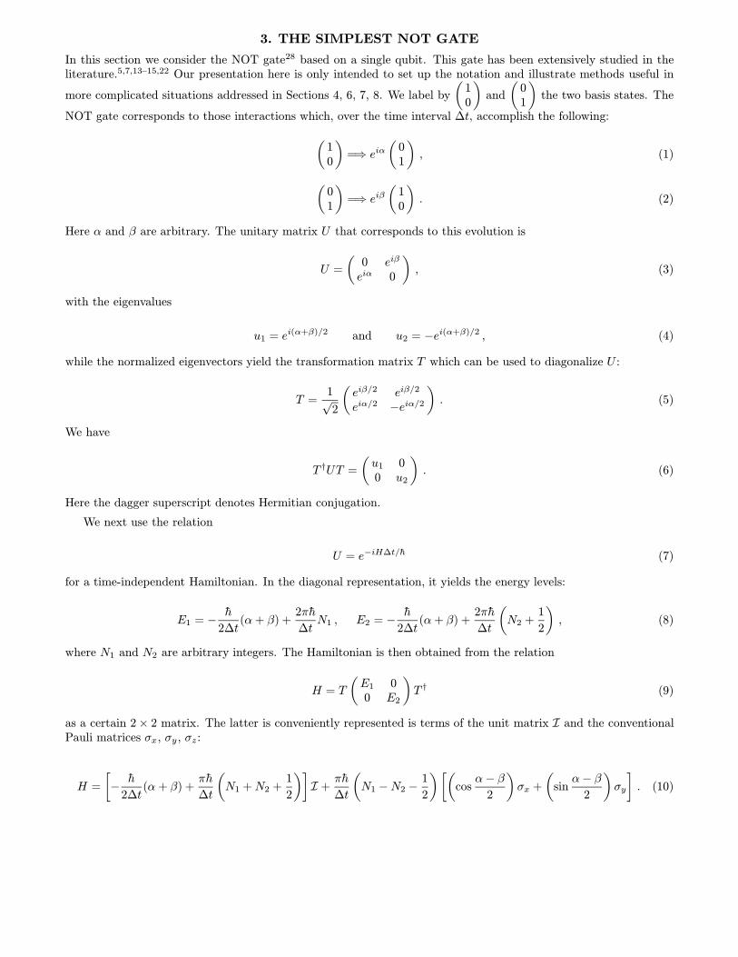
3. THE SIMPLEST NOT GATE

In this section we consider the NOT gate28 based on a single qubit. This gate has been extensively studied in theliterature.5,7,13–15,22 Our presentation here is only intended to set up the notation and illustrate methods useful in

more complicated situations addressed in Sections 4, 6, 7, 8. We label by

(10

)and

(01

)the two basis states. The

NOT gate corresponds to those interactions which, over the time interval ∆t, accomplish the following:(10

)=⇒ eiα

(01

), (1)

(01

)=⇒ eiβ

(10

). (2)

Here α and β are arbitrary. The unitary matrix U that corresponds to this evolution is

U =

(0 eiβ

eiα 0

), (3)

with the eigenvalues

u1 = ei(α+β)/2 and u2 = −ei(α+β)/2 , (4)

while the normalized eigenvectors yield the transformation matrix T which can be used to diagonalize U :

T =1√

2

(eiβ/2 eiβ/2

eiα/2 −eiα/2

). (5)

We have

T †UT =

(u1 00 u2

). (6)

Here the dagger superscript denotes Hermitian conjugation.

We next use the relation

U = e−iH∆t/h (7)

for a time-independent Hamiltonian. In the diagonal representation, it yields the energy levels:

E1 = −h

2∆t(α+ β) +

2πh

∆tN1 , E2 = −

h

2∆t(α+ β) +

2πh

∆t

(N2 +

1

2

), (8)

where N1 and N2 are arbitrary integers. The Hamiltonian is then obtained from the relation

H = T

(E1 00 E2

)T † (9)

as a certain 2× 2 matrix. The latter is conveniently represented is terms of the unit matrix I and the conventionalPauli matrices σx, σy , σz :

H =

[−

h

2∆t(α + β) +

πh

∆t

(N1 +N2 +

1

2

)]I +

πh

∆t

(N1 −N2 −

1

2

)[(cos

α− β

2

)σx +

(sin

α− β

2

)σy

]. (10)

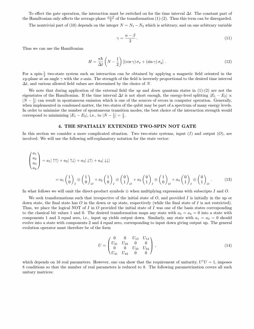
To effect the gate operation, the interaction must be switched on for the time interval ∆t. The constant part ofthe Hamiltonian only affects the average phase α+β

2 of the transformation (1)-(2). Thus this term can be disregarded.

The nontrivial part of (10) depends on the integer N = N1−N2 which is arbitrary, and on one arbitrary variable

γ =α− β

2. (11)

Thus we can use the Hamiltonian

H =πh

∆t

(N −

1

2

)[(cos γ)σx + (sin γ)σy] . (12)

For a spin- 12 two-state system such an interaction can be obtained by applying a magnetic field oriented in the

xy-plane at an angle γ with the x-axis. The strength of the field is inversely proportional to the desired time interval∆t, and various allowed field values are determined by the choice of N .

We note that during application of the external field the up and down quantum states in (1)-(2) are not theeigenstates of the Hamiltonian. If the time interval ∆t is not short enough, the energy-level splitting |E1 − E2| ∝|N − 1

2 | can result in spontaneous emission which is one of the sources of errors in computer operation. Generally,when implemented in condensed matter, the two states of the qubit may be part of a spectrum of many energy levels.In order to minimize the number of spontaneous transition modes, the best choice of the interaction strength wouldcorrespond to minimizing |E1 −E2|, i.e., to |N − 1

2 | =12 .

4. THE SPATIALLY EXTENDED TWO-SPIN NOT GATE

In this section we consider a more complicated situation. Two two-state systems, input (I) and output (O), areinvolved. We will use the following self-explanatory notation for the state vector:

a1

a2

a3

a4

= a1| ↑↑〉+ a2| ↑↓〉+ a3| ↓↑〉+ a4| ↓↓〉

= a1

(10

)I

⊗

(10

)O

+ a2

(10

)I

⊗

(01

)O

+ a3

(01

)I

⊗

(10

)O

+ a4

(01

)I

⊗

(01

)O

. (13)

In what follows we will omit the direct-product symbols ⊗ when multiplying expressions with subscripts I and O.

We seek transformations such that irrespective of the initial state of O, and provided I is initially in the up ordown state, the final state has O in the down or up state, respectively (while the final state of I is not restricted).Thus, we place the logical NOT of I in O provided the initial state of I was one of the basis states correspondingto the classical bit values 1 and 0. The desired transformation maps any state with a3 = a4 = 0 into a state withcomponents 1 and 3 equal zero, i.e., input up yields output down. Similarly, any state with a1 = a2 = 0 shouldevolve into a state with components 2 and 4 equal zero, corresponding to input down giving output up. The generalevolution operator must therefore be of the form

U =

0 0 U13 U14

U21 U22 0 00 0 U33 U34

U41 U42 0 0

, (14)

which depends on 16 real parameters. However, one can show that the requirement of unitarity, U †U = 1, imposes8 conditions so that the number of real parameters is reduced to 8. The following parametrization covers all suchunitary matrices:

U =

0 0 eiχ sin Ω eiβ cos Ω

−ei(α+ρ−η) sin Υ eiρ cos Υ 0 00 0 eiδ cos Ω −ei(β+δ−χ) sin Ω

eiα cos Υ eiη sin Υ 0 0

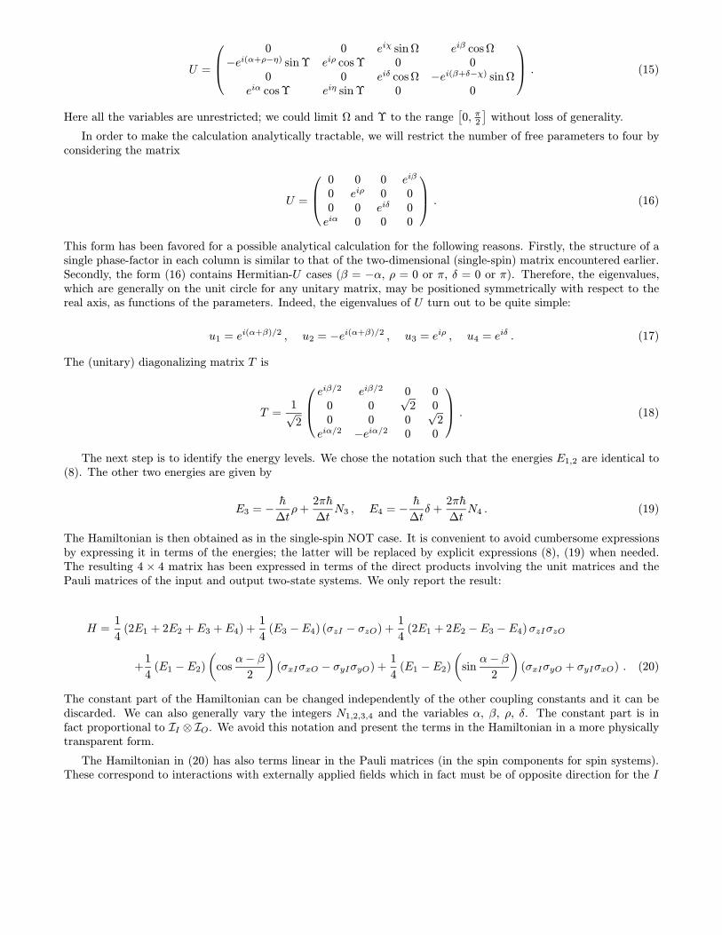
. (15)

Here all the variables are unrestricted; we could limit Ω and Υ to the range[0, π2

]without loss of generality.

In order to make the calculation analytically tractable, we will restrict the number of free parameters to four byconsidering the matrix

U =

0 0 0 eiβ

0 eiρ 0 00 0 eiδ 0eiα 0 0 0

. (16)

This form has been favored for a possible analytical calculation for the following reasons. Firstly, the structure of asingle phase-factor in each column is similar to that of the two-dimensional (single-spin) matrix encountered earlier.Secondly, the form (16) contains Hermitian-U cases (β = −α, ρ = 0 or π, δ = 0 or π). Therefore, the eigenvalues,which are generally on the unit circle for any unitary matrix, may be positioned symmetrically with respect to thereal axis, as functions of the parameters. Indeed, the eigenvalues of U turn out to be quite simple:

u1 = ei(α+β)/2 , u2 = −ei(α+β)/2 , u3 = eiρ , u4 = eiδ . (17)

The (unitary) diagonalizing matrix T is

T =1√

2

eiβ/2 eiβ/2 0 0

0 0√

2 00 0 0

√2

eiα/2 −eiα/2 0 0

. (18)

The next step is to identify the energy levels. We chose the notation such that the energies E1,2 are identical to(8). The other two energies are given by

E3 = −h

∆tρ+

2πh

∆tN3 , E4 = −

h

∆tδ +

2πh

∆tN4 . (19)

The Hamiltonian is then obtained as in the single-spin NOT case. It is convenient to avoid cumbersome expressionsby expressing it in terms of the energies; the latter will be replaced by explicit expressions (8), (19) when needed.The resulting 4 × 4 matrix has been expressed in terms of the direct products involving the unit matrices and thePauli matrices of the input and output two-state systems. We only report the result:

H =1

4(2E1 + 2E2 +E3 +E4) +

1

4(E3 −E4) (σzI − σzO) +

1

4(2E1 + 2E2 −E3 −E4)σzIσzO

+1

4(E1 −E2)

(cos

α− β

2

)(σxIσxO − σyIσyO) +

1

4(E1 −E2)

(sin

α− β

2

)(σxIσyO + σyIσxO) . (20)

The constant part of the Hamiltonian can be changed independently of the other coupling constants and it can bediscarded. We can also generally vary the integers N1,2,3,4 and the variables α, β, ρ, δ. The constant part is infact proportional to II ⊗ IO. We avoid this notation and present the terms in the Hamiltonian in a more physicallytransparent form.

The Hamiltonian in (20) has also terms linear in the Pauli matrices (in the spin components for spin systems).These correspond to interactions with externally applied fields which in fact must be of opposite direction for the I

and O spins. As explained in the introduction, we try to avoid such interactions: hopefully, external fields will onlybe used for clocking of the computation, i.e., for controlling the internal interactions via some intermediary part ofthe system connecting the I and O two-state systems. Thus, we will assume that E3 = E4 so that there are no termslinear is the spin components.

Among the remaining interaction terms, the term involving the z-components in the product form σzIσzO (≡σzI ⊗ σzO), has an arbitrary coefficient to be denoted −E . The terms of order two in the x and y components havefree parameters similar to those in (11)-(12). The final expression is

H = −EσzIσzO +πh

2∆t

(N −

1

2

)[(cos γ) (σxIσxO − σyIσyO) + (sin γ) (σxIσyO + σyIσxO)

]. (21)

Here N = N1 −N2 must be an integer. In order to minimize the spread of the energies E1 and E2 we could choose|N − 1

2 | =12 . Recall that we already have E3 = E4. Thus the energy levels of the Hamiltonian in (21) are

E1 = −E +πh

∆t

(N −

1

2

), E2 = −E −

πh

∆t

(N −

1

2

), E3,4 = E . (22)

Thus degeneracy of three levels (but not all four) can be achieved by varying the parameters.

The form of the interactions (21) is quite unusual as compared to the traditional spin-spin interactions in con-densed matter models. The latter usually are based on the uniaxial (Ising) interaction proportional to σzσz, or theplanar XY -model interaction proportional to σxσx + σyσy, or the isotropic (scalar-product) Heisenberg interaction.The spin components here are those of two different spins (not marked). The interaction (21) involves an unusuallyhigh degree of anisotropy in the system. The x and y components are coupled in a tensor form which presumablywill have to be realized in a medium with well-defined directionality, possibly, a crystal.

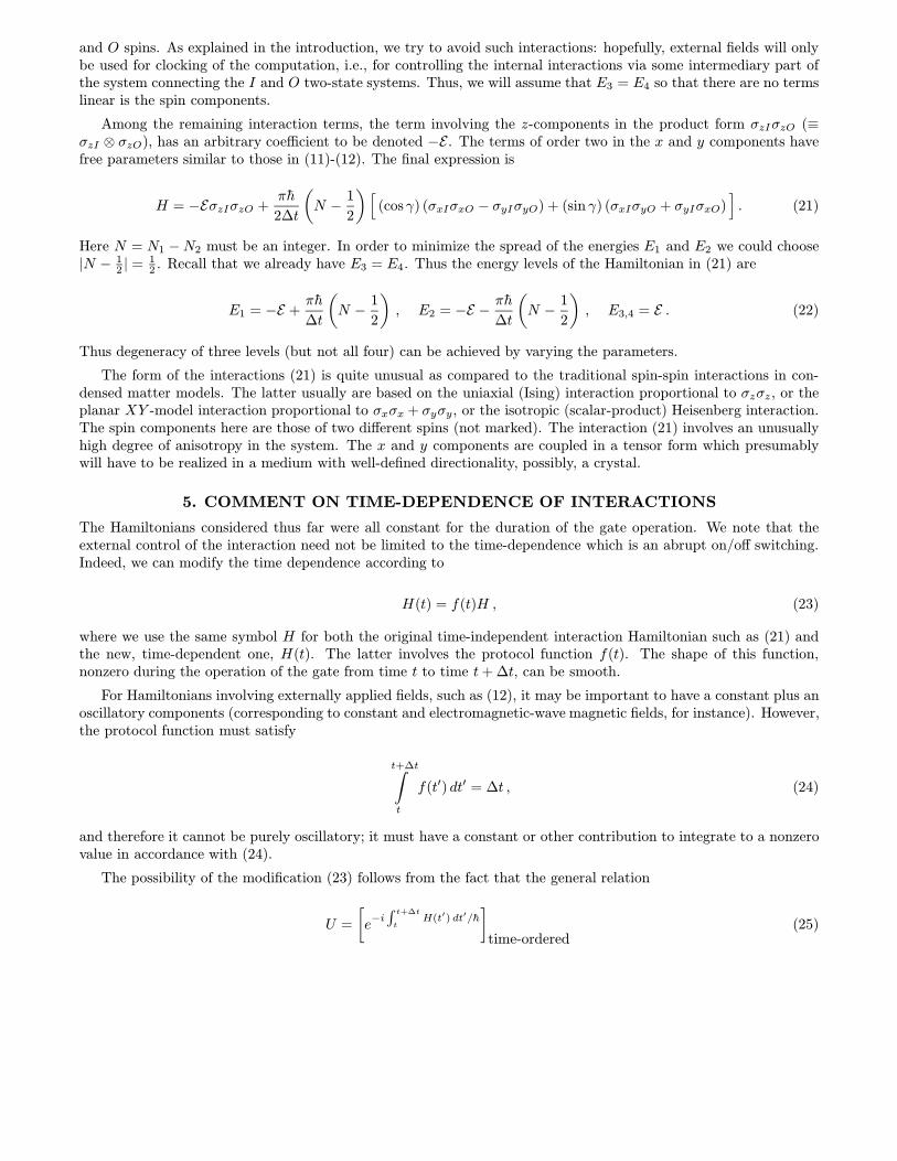
5. COMMENT ON TIME-DEPENDENCE OF INTERACTIONS

The Hamiltonians considered thus far were all constant for the duration of the gate operation. We note that theexternal control of the interaction need not be limited to the time-dependence which is an abrupt on/off switching.Indeed, we can modify the time dependence according to

H(t) = f(t)H , (23)

where we use the same symbol H for both the original time-independent interaction Hamiltonian such as (21) andthe new, time-dependent one, H(t). The latter involves the protocol function f(t). The shape of this function,nonzero during the operation of the gate from time t to time t+ ∆t, can be smooth.

For Hamiltonians involving externally applied fields, such as (12), it may be important to have a constant plus anoscillatory components (corresponding to constant and electromagnetic-wave magnetic fields, for instance). However,the protocol function must satisfy

t+∆t∫t

f(t′) dt′ = ∆t , (24)

and therefore it cannot be purely oscillatory; it must have a constant or other contribution to integrate to a nonzerovalue in accordance with (24).

The possibility of the modification (23) follows from the fact that the general relation

U =

[e−i∫ t+∆t

tH(t′) dt′/h

]time-ordered

(25)

does not actually require time ordering as long as the Hamiltonian commutes with itself at different times. Thiscondition is satisfied by (23). Furthermore, if the Hamiltonian can be written as a sum of commuting terms then eachterm can be multiplied by its own protocol function. Interestingly, the Hamiltonian of the paramagnetic-resonanceNOT gate14 is not of this form. It contains a constant part and an oscillatory part but they do not commute. Notethat the term proportional to E in (21) commutes with the rest of that Hamiltonian. The terms proportional to cos γand sin γ do not commute with each other. Rather, they anticommute, in (21), as such terms do in (12).

6. THE THREE-SPIN XOR GATE

Thus far we learned that extending the number of spins (qubits, two-state systems) involved in the NOT gate fromone to two produced an interaction Hamiltonian family (21) with structure that is quite new and unfortunately notsymmetric in terms of what we are used to in solid-state magnetic interactions. We will now consider a three-spinsystem: a quantum-XOR gate (which can also be realized10,30,43 with two spins). This choice is dictated by thefact that we can obtain analytical results and address a new issue that was not there for one- or two-spin systems:whether this quantum gate function can be accomplished with two-spin interactions.

We note that if a quantum logic operation is allowed to be decomposed into a sequence of unlimited number ofuniversal one- and two-spin gates then one can always reduce it to two-spin interactions.5,7,15,44 Here, however, weare interested in one-shot gates for which the external control involves the overall system Hamiltonian, over a singletime interval ∆t. The possibility of using solely two-spin interactions will actually depend on the logical functionand for more complicated systems it has to be explored by numerical studies. We note also that the issue of havingthe interactions short-range (e.g., nearest-neighbor) does not really arise for few-spin systems although it will be animportant design criterion as the number of spins (qubits) involved increases. Short-range two-particle interactionsare much better studied and accessible to experimental probe than multi-particle interactions.

We denote by A, B, C the three two-state systems, i.e., three spins (qubits). The transformation must be specifiedfor those initial states of the input spins A and B, at time t, that are one of the basis states |AB〉 = |11〉, |10〉, |01〉,or |00〉, where 1 and 0 denote the eigenstates of the z-components of the spin operators. Here 1 refers to the up stateand 0 refers to the down state; we use this notation for consistency with the classical bit notion. The initial state ofC is not specified. We would like to have a quantum evolution that mimics the XOR function:

A B output1 1 01 0 10 1 10 0 0

(26)

Here the output is at time t + ∆t. One way to accomplish this is to produce the output in A or B, i.e., work witha two-spin system where the input and output are the same. The Hamiltonian for such a system is not unique.Explicit examples can be found10,30 where XOR was obtained as a sub-result of the controlled-NOT gate operation.In the case of two spins involved, the interactions can be single- and two-spin only.

Here we require that the XOR result be put in C at time t + ∆t. The final states of A and B, as well as thephase of C are arbitrary. In fact, there are many different unitary transformations, U , that correspond to the desiredevolution in the eight-state space with the basis |ABC〉 = |111〉, |110〉, |101〉, |100〉, |011〉, |010〉, |001〉, |000〉. Thechoice of the transformation determines what happens when the initial state is a superposition of the reference states,what are the phases in the output, etc.

Let us consider first the following Hamiltonian31,32

H =πh

4∆t

(√2σzAσyB +

√2σzBσyC − σyBσxC

). (27)

It is written here in terms of the spin components; the subscripts A,B,C denote the spins. In the eight-state basisspecified earlier, its matrix can be obtained by direct product of the Pauli matrices and unit 2× 2 matrices I. Forinstance, the first interaction term is proportional to σzA ⊗ σyB ⊗ IC , This Hamiltonian involves only two-spin-component interactions. In fact, in this particular example A and C only interact with B.

One can show that the Hamiltonian (27) corresponds to the XOR result in C at t+ ∆t provided A and B werein one of the allowed superpositions of the appropriate binary states at t (we refer to superposition here becauseC is arbitrary at t). There are two ways to verify this.31,32 Firstly, one can diagonalize H and then calculate theevolution matrix U in the diagonal representation by using the general relation (7), valid for Hamiltonians which areconstant during the time interval ∆t, and then reverse the diagonalizing transformation.

The second, more general approach presented here is to design a whole family of two-spin-interaction Hamiltoniansof which the form (27) is but a special case, by analyzing generally a family of 8× 8 unitary matrices correspondingto the three-spin XOR gate. This program is carried out in Sections 7, 8.

7. THE STRUCTURE OF THE XOR UNITARY MATRIX AND HAMILTONIAN

We require any linear combination of the states |111〉 and |110〉 to evolve into a linear combination of |110〉, |100〉,|010〉, and |000〉; compare the underlined quantum numbers with the first entry in (26), with similar rules for theother three entries in (26). In the matrix notation, and in the standard basis |ABC〉 = |111〉, |110〉, |101〉, |100〉,|011〉, |010〉, |001〉, |000〉, the most general XOR evolution operator corresponding to the Boolean function (26), withthe output in C, is, therefore,

U =

0 0 U13 U14 U15 U16 0 0U21 U22 0 0 0 0 U27 U28

0 0 U33 U34 U35 U36 0 0U41 U42 0 0 0 0 U47 U48

0 0 U53 U54 U55 U56 0 0U61 U62 0 0 0 0 U67 U68

0 0 U73 U74 U75 U76 0 0U81 U82 0 0 0 0 U87 U88

. (28)

The condition of unitarity, UU † = 1, reduces the number of independent parameters but they are still too numerousfor the problem to be manageable analytically; we are going to consider a subset of operators of this form.

From our earlier discussion we know that one way to reduce the number of parameters and ensure unitarity isto keep a single phase factor in each column and row of the matrix. Some amount of lucky guessing is involvedin finding an analytically tractable parametrization. Thus, we choose a form which is diagonal in the states of theA-spin,

U =

(V4×4 04×4

04×4 W4×4

). (29)

Note that the input spins A and B are not treated symmetrically. Here 04×4 denotes the 4× 4 matrix of zeros. The4× 4 matrices V and W are parametrized as follows:

V =

0 0 eiδ 0eiα 0 0 00 0 0 eiβ

0 eiγ 0 0

, (30)

W =

0 eiρ 0 00 0 0 eiω

eiξ 0 0 00 0 eiη 0

. (31)

This choice of an 8-parameter unitary matrix U , see (29), was made because it has the structure

2U = (1 + σzA)V + (1− σzA)W = V +W + σzA(V −W ) , (32)

where V and W are operators in the space of B and C. Since U was chosen diagonal in the space of A, theHamiltonian, H, will have a similar structure,

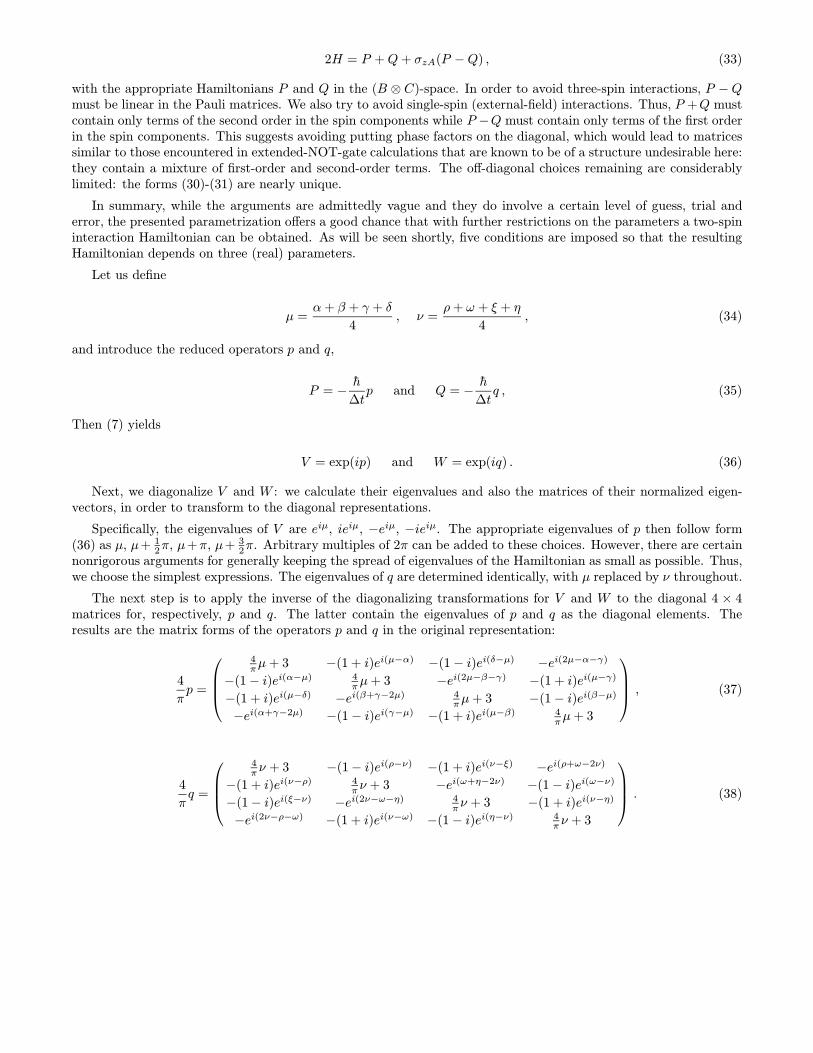
2H = P +Q+ σzA(P −Q) , (33)

with the appropriate Hamiltonians P and Q in the (B ⊗ C)-space. In order to avoid three-spin interactions, P −Qmust be linear in the Pauli matrices. We also try to avoid single-spin (external-field) interactions. Thus, P +Q mustcontain only terms of the second order in the spin components while P −Q must contain only terms of the first orderin the spin components. This suggests avoiding putting phase factors on the diagonal, which would lead to matricessimilar to those encountered in extended-NOT-gate calculations that are known to be of a structure undesirable here:they contain a mixture of first-order and second-order terms. The off-diagonal choices remaining are considerablylimited: the forms (30)-(31) are nearly unique.

In summary, while the arguments are admittedly vague and they do involve a certain level of guess, trial anderror, the presented parametrization offers a good chance that with further restrictions on the parameters a two-spininteraction Hamiltonian can be obtained. As will be seen shortly, five conditions are imposed so that the resultingHamiltonian depends on three (real) parameters.

Let us define

µ =α+ β + γ + δ

4, ν =

ρ+ ω + ξ + η

4, (34)

and introduce the reduced operators p and q,

P = −h

∆tp and Q = −

h

∆tq , (35)

Then (7) yields

V = exp(ip) and W = exp(iq) . (36)

Next, we diagonalize V and W : we calculate their eigenvalues and also the matrices of their normalized eigen-vectors, in order to transform to the diagonal representations.

Specifically, the eigenvalues of V are eiµ, ieiµ, −eiµ, −ieiµ. The appropriate eigenvalues of p then follow form(36) as µ, µ+ 1

2π, µ+π, µ+ 32π. Arbitrary multiples of 2π can be added to these choices. However, there are certain

nonrigorous arguments for generally keeping the spread of eigenvalues of the Hamiltonian as small as possible. Thus,we choose the simplest expressions. The eigenvalues of q are determined identically, with µ replaced by ν throughout.

The next step is to apply the inverse of the diagonalizing transformations for V and W to the diagonal 4 × 4matrices for, respectively, p and q. The latter contain the eigenvalues of p and q as the diagonal elements. Theresults are the matrix forms of the operators p and q in the original representation:

4

πp =

4πµ+ 3 −(1 + i)ei(µ−α) −(1− i)ei(δ−µ) −ei(2µ−α−γ)

−(1− i)ei(α−µ) 4πµ+ 3 −ei(2µ−β−γ) −(1 + i)ei(µ−γ)

−(1 + i)ei(µ−δ) −ei(β+γ−2µ) 4πµ+ 3 −(1− i)ei(β−µ)

−ei(α+γ−2µ) −(1− i)ei(γ−µ) −(1 + i)ei(µ−β) 4πµ+ 3

, (37)

4

πq =

4πν + 3 −(1− i)ei(ρ−ν) −(1 + i)ei(ν−ξ) −ei(ρ+ω−2ν)

−(1 + i)ei(ν−ρ) 4πν + 3 −ei(ω+η−2ν) −(1− i)ei(ω−ν)

−(1− i)ei(ξ−ν) −ei(2ν−ω−η) 4πν + 3 −(1 + i)ei(ν−η)

−ei(2ν−ρ−ω) −(1 + i)ei(ν−ω) −(1− i)ei(η−ν) 4πν + 3

. (38)

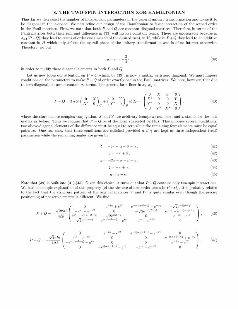
8. THE TWO-SPIN-INTERACTION XOR HAMILTONIAN

Thus far we decreased the number of independent parameters in the general unitary transformation and chose it tobe diagonal in the A-space. We now refine our design of the Hamiltonian to favor interaction of the second orderin the Pauli matrices. First, we note that both P and Q are constant-diagonal matrices. Therefore, in terms of thePauli matrices both their sum and difference in (33) will involve constant terms. These are undesirable because inσzA(P −Q) they lead to terms of order one (instead of the desired two), in H, while in P +Q they lead to an additiveconstant in H which only affects the overall phase of the unitary transformation and is of no interest otherwise.Therefore, we put

µ = ν = −3

4π , (39)

in order to nullify these diagonal elements in both P and Q.

Let us now focus our attention on P − Q which, by (39), is now a matrix with zero diagonal. We must imposeconditions on the parameters to make P −Q of order exactly one in the Pauli matrices. We note, however, that dueto zero-diagonal, it cannot contain σz terms. The general form liner in σx, σy is

P −Q = IB ⊗

(0 XX∗ 0

)C

+

(0 YY ∗ 0

)B

⊗ IC =

0 X Y 0X∗ 0 0 YY ∗ 0 0 X0 Y ∗ X∗ 0

, (40)

where the stars denote complex conjugation, X and Y are arbitrary (complex) numbers, and I stands for the unitmatrix as before. Thus we require that P − Q be of the form suggested by (40). This imposes several conditions:two above-diagonal elements of the difference must be equal to zero while the remaining four elements must be equalpairwise. One can show that these conditions are satisfied provided α, β, γ are kept as three independent (real)parameters while the remaining angles are given by

δ = −3π − α− β − γ , (41)

ρ = −π + β , (42)

ω = −2π − α− β − γ , (43)

ξ = −π + γ , (44)

η = π + α . (45)

Note that (39) is built into (41)-(45). Given this choice, it turns out that P +Q contains only two-spin interactions.We have no simple explanation of this property (of the absence of first-order terms in P +Q). It is probably relatedto the fact that the structure pattern of the original matrices V and W is quite similar even though the precisepositioning of nonzero elements is different. We find

P +Q = −

√2πhi

4∆t

0 e−iα + eiβ e−i(α+β+γ) − e−iγ −

√2e−i(α+γ)

−eiα − e−iβ 0 −√

2e−i(β+γ) e−iγ − e−i(α+β+γ)

eiγ − ei(α+β+γ)√

2ei(β+γ) 0 −e−iα − eiβ√2ei(α+γ) ei(α+β+γ) − eiγ eiα + e−iβ 0

, (46)

P −Q = −

√2πhi

4∆t

0 e−iα − eiβ e−i(α+β+γ) + e−iγ 0

−eiα + e−iβ 0 0 e−i(α+β+γ) + e−iγ

−ei(α+β+γ) − eiγ 0 0 e−iα − eiβ

0 −ei(α+β+γ) − eiγ −eiα + e−iβ 0

, (47)

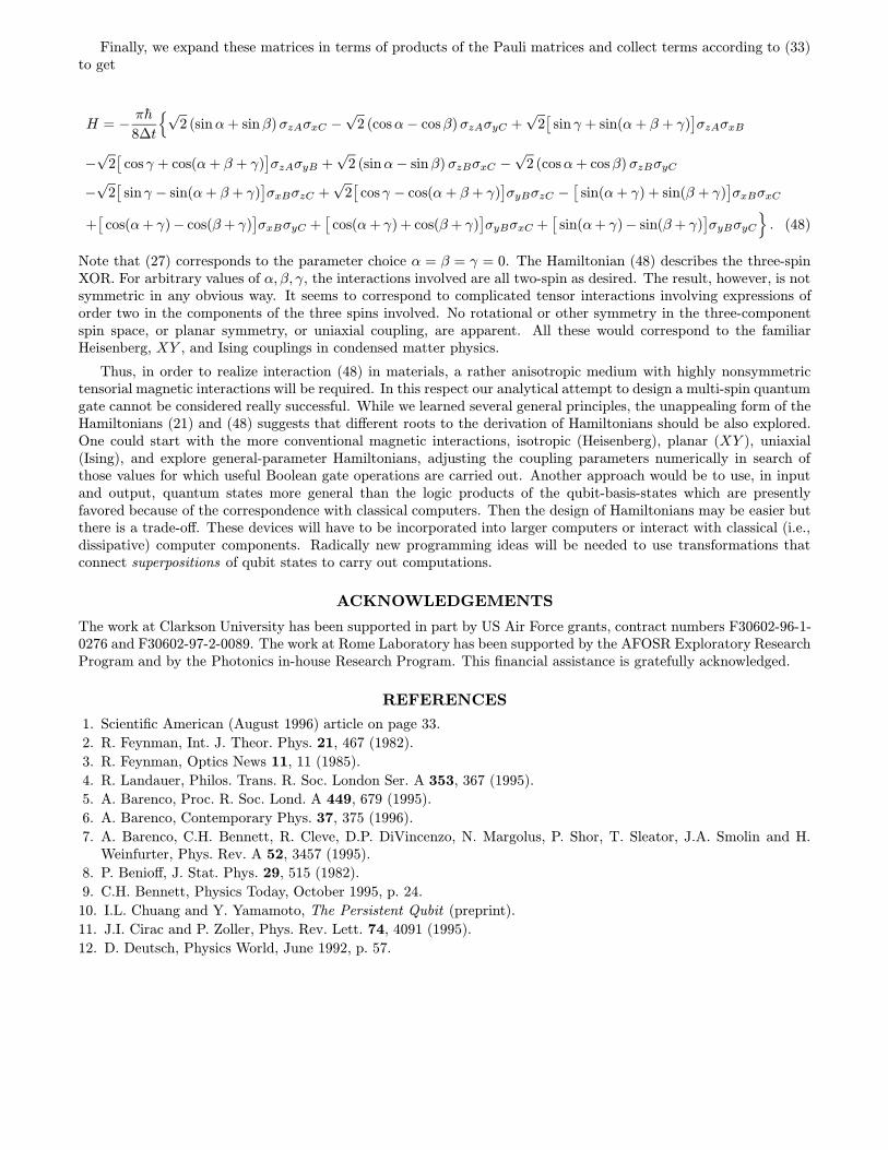
Finally, we expand these matrices in terms of products of the Pauli matrices and collect terms according to (33)to get

H = −πh

8∆t

√2 (sinα+ sinβ)σzAσxC −

√2 (cosα− cosβ)σzAσyC +

√2[

sin γ + sin(α+ β + γ)]σzAσxB

−√

2[

cos γ + cos(α+ β + γ)]σzAσyB +

√2 (sinα− sinβ) σzBσxC −

√2 (cosα+ cosβ) σzBσyC

−√

2[

sinγ − sin(α+ β + γ)]σxBσzC +

√2[

cos γ − cos(α+ β + γ)]σyBσzC −

[sin(α+ γ) + sin(β + γ)

]σxBσxC

+[

cos(α+ γ)− cos(β + γ)]σxBσyC +

[cos(α+ γ) + cos(β + γ)

]σyBσxC +

[sin(α+ γ)− sin(β + γ)

]σyBσyC

. (48)

Note that (27) corresponds to the parameter choice α = β = γ = 0. The Hamiltonian (48) describes the three-spinXOR. For arbitrary values of α, β, γ, the interactions involved are all two-spin as desired. The result, however, is notsymmetric in any obvious way. It seems to correspond to complicated tensor interactions involving expressions oforder two in the components of the three spins involved. No rotational or other symmetry in the three-componentspin space, or planar symmetry, or uniaxial coupling, are apparent. All these would correspond to the familiarHeisenberg, XY , and Ising couplings in condensed matter physics.

Thus, in order to realize interaction (48) in materials, a rather anisotropic medium with highly nonsymmetrictensorial magnetic interactions will be required. In this respect our analytical attempt to design a multi-spin quantumgate cannot be considered really successful. While we learned several general principles, the unappealing form of theHamiltonians (21) and (48) suggests that different roots to the derivation of Hamiltonians should be also explored.One could start with the more conventional magnetic interactions, isotropic (Heisenberg), planar (XY ), uniaxial(Ising), and explore general-parameter Hamiltonians, adjusting the coupling parameters numerically in search ofthose values for which useful Boolean gate operations are carried out. Another approach would be to use, in inputand output, quantum states more general than the logic products of the qubit-basis-states which are presentlyfavored because of the correspondence with classical computers. Then the design of Hamiltonians may be easier butthere is a trade-off. These devices will have to be incorporated into larger computers or interact with classical (i.e.,dissipative) computer components. Radically new programming ideas will be needed to use transformations thatconnect superpositions of qubit states to carry out computations.

ACKNOWLEDGEMENTS

The work at Clarkson University has been supported in part by US Air Force grants, contract numbers F30602-96-1-0276 and F30602-97-2-0089. The work at Rome Laboratory has been supported by the AFOSR Exploratory ResearchProgram and by the Photonics in-house Research Program. This financial assistance is gratefully acknowledged.

REFERENCES

1. Scientific American (August 1996) article on page 33.

2. R. Feynman, Int. J. Theor. Phys. 21, 467 (1982).

3. R. Feynman, Optics News 11, 11 (1985).

4. R. Landauer, Philos. Trans. R. Soc. London Ser. A 353, 367 (1995).

5. A. Barenco, Proc. R. Soc. Lond. A 449, 679 (1995).

6. A. Barenco, Contemporary Phys. 37, 375 (1996).

7. A. Barenco, C.H. Bennett, R. Cleve, D.P. DiVincenzo, N. Margolus, P. Shor, T. Sleator, J.A. Smolin and H.Weinfurter, Phys. Rev. A 52, 3457 (1995).

8. P. Benioff, J. Stat. Phys. 29, 515 (1982).

9. C.H. Bennett, Physics Today, October 1995, p. 24.

10. I.L. Chuang and Y. Yamamoto, The Persistent Qubit (preprint).

11. J.I. Cirac and P. Zoller, Phys. Rev. Lett. 74, 4091 (1995).

12. D. Deutsch, Physics World, June 1992, p. 57.

13. D. Deutsch, A. Barenco and A. Ekert, Proc. R. Soc. Lond. A 449, 669 (1995).

14. D.P. DiVincenzo, Science 270, 255 (1995).

15. D.P. DiVincenzo, Phys. Rev. A 51, 1015 (1995).

16. A. Ekert, Quantum Computation (preprint).

17. A. Ekert and R. Jozsa, Rev. Mod. Phys. 68, 733 (1996).

18. S. Haroche and J.-M. Raimond, Physics Today, August 1996, p. 51.

19. S.P. Hotaling, Radix-R > 2 Quantum Computation (preprint).

20. S. Lloyd, Science 261, 1563 (1993).

21. N. Margolus, Parallel Quantum Computation (preprint).

22. A. Peres, Phys. Rev. A 32, 3266 (1985).

23. D.R. Simon, On the Power of Quantum Computation (preprint).

24. A. Steane, The Ion Trap Quantum Information Processor (preprint).

25. B. Schumacher, Phys. Rev. A 51, 2738 (1995).

26. B. Schwarzschild, Physics Today, March 1996, p. 21.

27. W.H. Zurek, Phys. Rev. Lett. 53, 391 (1984).

28. D. Mozyrsky, V. Privman and S.P. Hotaling, Design of Gates for Quantum Computation: the NOT Gate(preprint).

29. D. Mozyrsky and V. Privman, Quantum Signal Splitting that Avoids Initialization of the Targets (preprint).

30. D. Mozyrsky, V. Privman and M. Hillery, A Hamiltonian for Quantum Copying, Phys. Lett. A, in press.

31. D. Mozyrsky, V. Privman and S.P. Hotaling, Extended Quantum XOR Gate in Terms of Two-Spin Interactions(preprint).

32. D. Mozyrsky, V. Privman and S.P. Hotaling, Design of Gates for Quantum Computation: the Three-Spin XORin Terms of Two-Spin Interactions (preprint).

33. I.L. Chuang, R. Laflamme, P.W. Shor and W.H. Zurek, Science 270, 1633 (1995).

34. C. Durr and P. Høyer, A Quantum Algorithm for Finding the Minimum (preprint).

35. R.B. Griffiths and C.-S. Niu, Semiclassical Fourier Transform for Quantum Computation (preprint).

36. L.K. Grover, A Fast Quantum Mechanical Algorithm for Estimating the Median (preprint).

37. P.W. Shor, Algorithms for Quantum Computation: Discrete Log and Factoring. Extended Abstract (preprint).

38. E. Knill and R. Laflamme, A Theory of Quantum Error-Correcting Codes (preprint).

39. W.G. Unruh, Phys. Rev. A 51, 992 (1995).

40. D.P. DiVincenzo, Topics in Quantum Computers (preprint).

41. R. Laflamme, C. Miguel, J.P. Paz and W.H. Zurek, Phys. Rev. Lett. 77, 198 (1996).

42. A. Ekert and C. Macchiavello, Phys. Rev. Lett. 77, 2585 (1996).

43. D. Loss and D.P. DiVincenzo, Quantum Computation with Quantum Dots (preprint).

44. S. Lloyd, Phys. Rev. Lett. 75, 346 (1995).

45. C. Monroe, D.M. Meekhof, B.E. King, W.M. Itano and D.J. Wineland, Phys. Rev. Lett. 75, 4714 (1995).

46. Q. Turchette, C. Hood, W. Lange, H. Mabushi and H.J. Kimble, Phys. Rev. Lett. 75, 4710 (1995).

This article will be published in the Proceedings of the Conference “Photonic Quantum Computing.AeroSense 97” (SPIE—The International Society for Optical Engineering, 1997), SPIE ProceedingsVolume number 3076.