Accepted Manuscript

Habit persistence and the long-run labor supply

Clemens C. Struck

PII: S0165-1765(14)00204-3DOI: http://dx.doi.org/10.1016/j.econlet.2014.05.027Reference: ECOLET 6360

To appear in: Economics Letters

Received date: 24 March 2014Revised date: 22 May 2014Accepted date: 26 May 2014

Please cite this article as: Struck, C.C., Habit persistence and the long-run labor supply.Economics Letters (2014), http://dx.doi.org/10.1016/j.econlet.2014.05.027

This is a PDF file of an unedited manuscript that has been accepted for publication. As aservice to our customers we are providing this early version of the manuscript. The manuscriptwill undergo copyediting, typesetting, and review of the resulting proof before it is published inits final form. Please note that during the production process errors may be discovered whichcould affect the content, and all legal disclaimers that apply to the journal pertain.

1. Standard macroeconomic models predict that a permanent increase in income causes a declinein the number of hours worked

2. I provide time series, cross country and micro evidence that there is no relationship betweenincome and labor hours worked

3. I show that the intertemporal elasticity of substitution (IES) is the key driving parameter in astandard neoclassical model

4. I show that both internal and external habit persistence can resolve this puzzle independent ofthe IES

1

*Highlights (for review)

Habit Persistence and the Long-Run Labor Supply∗

Clemens C. Struck†

May 22, 2014

Abstract

Standard macroeconomic models possess the undesirable feature that people stop working inthe long run. Assuming standard parameters, the neoclassical model predicts that 2% of annualproductivity growth leads to a 99% decline in the labor supply after 624 years. Yet, this contradictsthe fact that labor hours per capita are relatively stable, even over a long period of time. Thispaper shows how internal and external habit persistence each work to stabilize the long run laborsupply, independent of key parameter choices.

JEL: E13, E20, E24Keywords: Habit Formation, Labor Supply

1 Introduction

In 1930, John M. Keynes envisaged that the generation of his grandchildren would only work three

hours a day. Underlying this prediction is a reasoning that is engrained in many of today’s macroe-

conomic models: when people become richer, their propensity to consume more rapidly declines. As

a result of the deficiency of more consumption to further satisfy people’s needs, they choose to work

less. This reasoning has, however, not proven reliable. Despite the increase in income, U.S. aggregate

labor hours per capita have remained relatively stable over the past 60 years (Figure 1). People in

richer countries do not work less than people in poorer countries (Figure 2). Richer people in the

U.S. do not work less than poorer people (Figure 3). The empirical evidence therefore raises a simple

question: why do people still work so much?

This paper shows how internal and external habit persistence each work to stabilize the long

run labor supply, independent of key parameter choices. It nails down the theoretical problem which

underpins the right choice of the consumption utility function. It shows the irrelevance of the choice of

the labor disutility function. In both approaches the standard consumption utility function is replaced

by a new function. Both approaches share the idea that what matters for utility is the distance from∗I am grateful to Paul Scanlon and Michael Wycherley for insightful discussions and valuable suggestions. I also

thank Brendan Epstein and Miles Kimball for helpful comments.†Department of Economics, Trinity College Dublin, Ireland, email: struckc@tcd.ie; Department of Economics, Yale

University, USA, email: clemens.struck@yale.edu

1

*ManuscriptClick here to view linked References

1950 1960 1970 1980 1990 2000 20100

200

400

600

800

1000

1200

1400

1600

Ann

ual L

abor

Hou

rs p

er C

apita

Figure 1: Total U.S. Employee Hours per Capita 1948-2011. Note: The number of employee hoursworked and the number of persons are taken from the U.S. Bureau of Economic Analysis (BEA).

500 600 700 800 900 1000 1100 12000

5

10

15

20

25

30

35

40

Annual Labor Hours per Capita

Rea

l PP

P C

onsu

mpt

ion

per

Cap

ita

corr=0.163

Figure 2: Consumption and Labor Hours across countries. Note: 31 countries, 2000-2007 averages.The data are taken from the Organisation for Economic Co-operation and Development (OECD).

0 500 1000 1500 2000 2500 3000 3500 4000 4500 50000

100

200

300

400

500

Annual Labor Hours

Com

pens

atio

n pe

r H

our

corr=−0.002

Figure 3: Labor Hours and Wage Rate. Note: 6541 families. Labor hours are the family head’s totalhours of work in 2006. The wage rate is the family head’s hourly wage. Data are taken from the PanelStudy of Income Dynamics (PSID).

2

a reference point - not the level of consumption per se. In the first approach, the reference point is the

level of past consumption. In the second approach, the reference point is the level of consumption of

other consumers. Because these reference points move with the level of consumption over time (when

past consumption rises; when other consumers become wealthier and consume more), marginal utility

from consumption does not fall as fast as in the model with standard preferences. Habit persistence

therefore prevents the consumers from rapidly losing their appetite for consumption. The propensity

to consume further still falls in the level of consumption as absolute deviations from the reference

point become less important.

This paper contributes to the literature that attempts to reconcile estimates of a low intertemporal

elasticity of substitution with stable labor hours. It is closely related to Scanlon (2013) who shows how

new goods can provide additional motivation for consumption. It differs from Scanlon in that it reveals

an alternative mechanism - habit persistence - that provides additional motivation for consumption

independent of the intertemporal elasticity of substitution. It is further related to Epstein and Kimball

(2013) who argue that increases in job utility keep labor hours stable. This literature contrasts with

explanations of stable labor hours that rely on an intertemporal elasticity of substitution of unity.

These explanations are in conflict with empirical evidence that suggests an intertemporal elasticity

of substitution that is significantly below unity. Hall (1988), Basu and Kimball (2002) and Kimball

et al. (2009) among others provide evidence that the intertemporal elasticity of substitution is closer

to zero than to unity. In terms of modeling habit persistence this paper follows Abel (1990). Abel

uses habit persistence to account for the equity premium puzzle.

The rest of the paper is organized as follows. Section 2 derives the condition for stable labor hours

and shows how the standard model fails to satisfy it, but that habit persistence satisfies it independent

of key parameter choices. Section 3 simulates the theories and compares them to actual data. Section

4 concludes the paper.

2 Theory

2.1 Firms

The representative firm maximizes profits

AtKαt L

1−αt − wtLt − rtKt (1)

where At denotes the total factor productivity at time t, α ∈ [0, 1] the share of capital, Kt the

capital stock, Lt the labor supply, wt the wage and rt the return to capital. The economy is subject

to exogenous changes in the productivity A which grows at rate g. The firm’s first order with respect

to capital and labor yield:

3

wt = (1− α)A1

1−αt

[rtα

] αα−1

(2)

Kt = A1

1−αt

[rtα

] 1α−1

Lt (3)

2.2 Consumers

The representative consumer maximizes lifetime utility Ut which is given by

Ut =∞∑

j=0

βj [u(Ct+j)− v(Lt+j)] (4)

subject to

i) a budget constraint: wtLt + rtKt = Ct + It

ii) a capital accumulation equation: Kt+1 = (1− δ)Kt + It

Utility from consumption, u, is a concave function. Disutility from work v is a convex function.

Aggregate utility U is additively separable in consumption and labor1

The consumer optimality conditions with respect to Lt and Ct imply

wtwt−1

u′(Ct)u′(Ct−1)

=v′(Lt)v′(Lt−1)

. (5)

Consumer optimization with respect to Kt+1 and It implies the following equilibrium condition:

r =1β− 1 + δ. (6)

2.3 The condition for a stable long run labor supply

This section shows that there is a unique condition for a long run stable labor supply that needs to

be satisfied. Suppose L is constant, then the equilibrium condition (5) becomes independent of the

function, v, and reduces to:

wtwt−1

=u′(Ct−1)u′(Ct)

(7)

In other words, L is only constant when this equation holds.

PROPOSITION 1: The labor supply, L, is constant if and only if wage growth equals the inverse

of marginal consumption utility growth - independent of the choice of the labor disutility function.1An alternative specification where utility is non-separable, i.e. labor and consumption are complements, could

potentially serve as an explanation of long run stable labor hours as Basu and Kimball (2002) show. However, Campbelland Ludvigson (2001) point out that evidence for non-separability is weak at best.

4

Substituting into the consumer budget constraint the equilibrium conditions for wt, rt, Kt and

using It = δKt yields

Ct = A1

1−αt Lt

[(1− α)

[ rα

] αα−1

+ (r − δ)[ rα

] 1α−1]

(8)

PROPOSITION 2: If L is constant, both, consumption and wages, grow at the same rate,

[At/At−1]1

1−α - independent of the choice of the consumption utility function.

Propositions 1 and 2 together imply that, for L to be stable, the following equation must hold:

u′(Ct−1)u′(Ct)

=CtCt−1

(9)

2.4 The problem with standard preferences

Under standard preferences,

u(Ct) =C1−φt

1− φ (10)

equation Eq. (9) holds if and only if φ = 1. This is, however, at odds with the micro and macro

evidence in the literature that suggests that the intertemporal elasticity of substitution (IES), 1/φ,

is below 1. In postwar U.S. data, Hall (1988) finds that the IES is ”unlikely to be much above 0.1

and may well be zero”. Patterson and Pesaran (1992) generally confirm Hall’s result of an IES well

below 1. Using IV estimation techniques they find an upper bound of 0.4 for the IES in postwar U.S.

and UK data. In a cross country sample, Campbell (2003) confirms these results of an intertemporal

elasticity of substitution below 0.5. Yogo (2004) finds the IES to be 0.2 in the U.S. and not higher

than 0.5 in other developed countries. Based on U.S. Consumer Expenditure Survey (CEX) data,

Vissing-Jorgensen (2002) finds that the IES differs for stock- and bondholders, but is significantly

below 1 in both cases. Based on survey respondents’ choices in hypothetical situations, Barsky et al.

(1997) find that ”virtually no respondents have intertemporal substitution as elastic as that implied

by log utility” and a mean elasticity of intertemporal substitution of 0.2.2

2Log utility is a special case of Eq. (10) when φ = 1.

5

2.5 How reference-based preferences resolve the problem

This section shows how two alternative theories can each satisfy the condition for stable labor hours,

Eq. (9), independent of the intertemporal elasticity of substitution. Both theories follow Abel (1990)

in terms of modelling utility. Under internal habit persistence,

u(Ct, Ct−1) =

[Ct

aCt−1

]1−φ

1− φ (11)

the consumer first order conditions imply that Eq. (9) is satisfied if

u′(Ct, Ct−1, Ct−2)u′(Ct+1, Ct, Ct−1)

=C−φt−1/a

1−φC1−φt−2 − βC1−φ

t /a1−φC2−φt−1

C−φt /a1−φC1−φt−1 − βC1−φ

t+1 /a1−φC2−φ

t

=CtCt−1

(12)

This equation holds without any parameter constraints as long as Ct+1 ≈ Ct ≈ Ct−1 ≈ Ct−2,

which is approximately true in the long run: the aggregate level of real consumption per capita in

100 years in time should be very similar to the level of consumption in 98, 99 and 101 years. Under,

external habit persistence there are two symmetric consumers, n and m. The utility of consumer n is

given by

un(Cnt , Cmt ) =

[CntaCmt

]1−φ

1− φ (13)

the consumer first order conditions imply that Eq. (9) is satisfied if

u′n(Cnt−1, Cmt−1)

u′n(Cnt , Cmt )=C−φn,t−1/a

1−φC1−φm,t−1

C−φnt /a1−φC1−φmt

=CntCnt−1

(14)

This equation holds without any parameter constraints, because consumers are symmetric and,

thus, Cn = Cm. In both frameworks is the intertemporal elasticity of substitution given by

− uCuCC

1C

=1φ. (15)

The choice of the intertemporal elasticity of substitution is irrelevant because internal and external

habit persistence can generate stable labor hours independent of φ. How plausible are reference

based preferences? Rayo and Becker (2007) emphasize that a utility function that combines habits

with peer comparisons has biological foundations and helps to account for several empirical findings

including the Easterlin Paradox, Easterlin (1995). Luttmer (2005) finds that self-reported happiness

is related to earnings of neighbors. Reference based preferences are also widely used throughout the

literature. Carroll et al. (2000) show that the positive saving and growth correlation can be explained

with habit persistence in preferences. Boivin and Giannoni (2006), Fuhrer (2000), Christiano et al.

(2005) among others use habit persistence in models of monetary policy. Uhlig (2007), Campbell and

6

Cochrane (1999), Campbell and Cochrane (2000) and Hyde and Sherif (2010) among others employ

habit persistence to increase the asset price volatility of their models.

3 Simulations

This section estimates the aggregate U.S. labor hours compares them to actual data. To back out the

labor hours, I have to assume a specific functional form for v(L). Following a review of the literature

by Wallenius and Prescott (2011), I use the standard functional form,

vt =L1+φLt

1 + φL(16)

Where φL is the inverse of the intertemporal elasticity of substitution of labor supply. I estimate

the labor supply based on Eq. (5):

L̂t = Lt−1

[wtwt−1

u′tu′t−1

] 1φL

(17)

Initially, I normalize L = 1. I use 5-year averaged data from the Bureau of Economic Analysis

(BEA) for w and C. To calculate wt, I take the aggregate compensation received by employees in

year t and divide it by the aggregate number of hours worked by full-time and part-time employees.

C is simply the aggregate consumption per capita. I divide both, w and C, by the BEA price index.

u′t/u′t−1 is

i) C−φtC−φt−1

(standard preferences)

ii)C−φt−1/a

1−φC1−φt−2 −βC

1−φt /a1−φC2−φ

t−1

C−φt /a1−φC1−φt−1 −βC

1−φt+1 /a

1−φC2−φt

(internal habit persistence)

iii) C−φnt /C1−φmt

C−φn,t−1/C1−φm,t−1

(external habit persistence)

I set 1/φ = 0.5 - a value at the top end of the range for the IES, as discussed above. A lower IES

results in a greater fall of labor hours in the standard model but does not change the labor supply

response when preferences are reference, based as shown above. I set β = 0.97. Following Prescott

(2004) who estimates that the elasticity of labor supply is rather large, I set φL = 2. As Proposition

1 shows, the choice of φL is irrelevant in explaining the long run stability of labor hours. To see

why, the main term on the right hand side of Eq. (17), wtwt−1

u′tu′t−1

, must equal 1 to keep L stable over

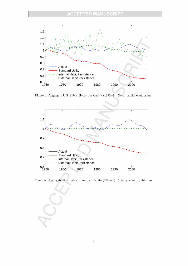
time. Figure 4 plots the development of the aggregate labor supply in the U.S. during 1950-2009. In

the standard model, the labor supply falls by nearly 50% relative to actual data. Both, internal and

external habit persistence, are close to the actual data in terms of replicating the stable long run labor

supply. The labor supply under habit persistence is, however, much more volatile than under external

habit persistence. One cause for this high volatility is that the habit is last year’s consumption and

7

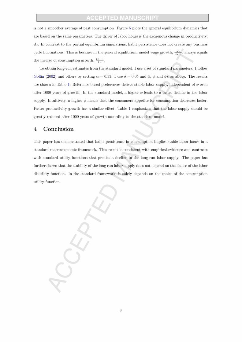
is not a smoother average of past consumption. Figure 5 plots the general equilibrium dynamics that

are based on the same parameters. The driver of labor hours is the exogenous change in productivity,

At. In contrast to the partial equilibrium simulations, habit persistence does not create any business

cycle fluctuations. This is because in the general equilibrium model wage growth, wtwt−1

, always equals

the inverse of consumption growth, Ct−1Ct

.

To obtain long-run estimates from the standard model, I use a set of standard parameters. I follow

Gollin (2002) and others by setting α = 0.33. I use δ = 0.05 and β, φ and φL as above. The results

are shown in Table 1. Reference based preferences deliver stable labor supply, independent of φ even

after 1000 years of growth. In the standard model, a higher φ leads to a faster decline in the labor

supply. Intuitively, a higher φ means that the consumers appetite for consumption decreases faster.

Faster productivity growth has a similar effect. Table 1 emphasizes that the labor supply should be

greatly reduced after 1000 years of growth according to the standard model.

4 Conclusion

This paper has demonstrated that habit persistence in consumption implies stable labor hours in a

standard macroeconomic framework. This result is consistent with empirical evidence and contrasts

with standard utility functions that predict a decline in the long-run labor supply. The paper has

further shown that the stability of the long run labor supply does not depend on the choice of the labor

disutility function. In the standard framework, it solely depends on the choice of the consumption

utility function.

8

1950 1960 1970 1980 1990 20000.5

0.6

0.7

0.8

0.9

1

1.1

1.2

1.3

ActualStandard UtilityInternal Habit PersistenceExternal Habit Persistence

Figure 4: Aggregate U.S. Labor Hours per Capita (1950=1). Note: partial equilibrium.

1950 1960 1970 1980 1990 20000.6

0.7

0.8

0.9

1

1.1

ActualStandard UtilityInternal Habit PersistenceExternal Habit Persistence

Figure 5: Aggregate U.S. Labor Hours per Capita (1950=1). Note: general equilibrium.

9

Table 1: The Labor Supply in the Standard Model

2% productivity growth p.a.

Initial 100 years 500 years 1000 years

Standard Preferences, φ = 2 100.00 % 48.12 % 2.50 % 0.06 %Standard Preferences, φ = 4 100.00 % 23.15 % 0.06 % 0.00 %

1% productivity growth p.a.

Initial 100 years 500 years 1000 years

Standard Preferences, φ = 2 100.00 % 69.24 % 15.68 % 2.45 %Standard Preferences, φ = 4 100.00 % 47.94 % 2.46 % 0.06 %

10

References

Abel, A. B. (1990). Asset prices under habit formation and catching up with the joneses. American EconomicReview, 80(2):38–42.

Barsky, R. B., Juster, F. T., Kimball, M. S., and Shapiro, M. D. (1997). Preference parameters and behavioralheterogeneity: An experimental approach in the health and retirement study. The Quarterly Journal ofEconomics, 112(2):537–579.

Basu, S. and Kimball, M. S. (2002). Long-run labor supply and the elasticity of intertemporal substitutionfor consumption. Boston College and University of Michigan: unpublished manuscript.

Boivin, J. and Giannoni, M. P. (2006). Has monetary policy become more effective? The Review of Economicsand Statistics, 88(3):445–462.

Campbell, J. Y. (2003). Consumption-based asset pricing, volume 1, pages 803–887. Elsevier.

Campbell, J. Y. and Cochrane, J. (1999). Force of habit: A consumption-based explanation of aggregate stockmarket behavior. Journal of Political Economy, 107(2):205–251.

Campbell, J. Y. and Cochrane, J. H. (2000). Explaining the poor performance of consumption-based assetpricing models. Journal of Finance, 55(6):2863–2878.

Campbell, J. Y. and Ludvigson, S. (2001). Elasticities of substitution in real business cycle models with homeprotection. Journal of Money, Credit and Banking, 33(4):847–75.

Carroll, C. D., Overland, J., and Weil, D. N. (2000). Saving and growth with habit formation. AmericanEconomic Review, 90(3):341–355.

Christiano, L. J., Eichenbaum, M., and Evans, C. L. (2005). Nominal rigidities and the dynamic effects of ashock to monetary policy. Journal of Political Economy, 113(1):1–45.

Easterlin, R. A. (1995). Will raising the incomes of all increase the happiness of all? Journal of EconomicBehavior & Organization, 27(1):35–47.

Epstein, B. and Kimball, M. S. (2013). The decline of drudgery and the paradox of hard work. University ofMichigan: unpublished manuscript.

Fuhrer, J. C. (2000). Habit formation in consumption and its implications for monetary-policy models.American Economic Review, 90(3):367–390.

Gollin, D. (2002). Getting income shares right. Journal of Political Economy, 110(2):458–474.

Hall, R. E. (1988). Intertemporal substitution in consumption. Journal of Political Economy, 96(2):339–57.

Hyde, S. and Sherif, M. (2010). Consumption asset pricing and the term structure. The Quarterly Review ofEconomics and Finance, 50(1):99–109.

John Maynard Keynes, E. J. and Moggridge, D. (1978). Economic Possibilities for our Grandchildren (1930),volume The Collected Writings of John Maynard Keynes The Collected Writings of John Maynard Keynes.Royal Economic Society.

Kimball, M. S., Sahm, C. R., and Shapiro, M. D. (2009). Risk preferences in the psid: Individual imputationsand family covariation. American Economic Review, 99(2):363–68.

Luttmer, E. F. P. (2005). Neighbors as negatives: Relative earnings and well-being. The Quarterly Journalof Economics, 120(3):963–1002.

Patterson, K. D. and Pesaran, B. (1992). The intertemporal elasticity of substitution in consumption in theunited states and the united kingdom. The Review of Economics and Statistics, 74(4):573–84.

Prescott, E. C. (2004). Why do americans work so much more than europeans? Technical Report 10316.

Rayo, L. and Becker, G. S. (2007). Habits, peers, and happiness: An evolutionary perspective. AmericanEconomic Review, 97(2):487–491.

Scanlon, P. (2013). Why do people work so hard? Trinity College, Dublin: unpublished manuscript.

Uhlig, H. (2007). Explaining asset prices with external habits and wage rigidities in a dsge model. AmericanEconomic Review, 97(2):239–243.

11

Vissing-Jorgensen, A. (2002). Limited asset market participation and the elasticity of intertemporal substitu-tion. Journal of Political Economy, 110(4):825–853.

Wallenius, J. and Prescott, E. C. (2011). Aggregate labor supply. Technical Report 457.

Yogo, M. (2004). Estimating the elasticity of intertemporal substitution when instruments are weak. TheReview of Economics and Statistics, 86(3):797–810.

12