Embed Size (px)
Citation preview

WORLD BANK TECHNICAL PAPER NUMBER 46
Guidelines for Conducting and Calibrating Road Roughness Measurements
Michael W Sayers, Thomas D. Gillespie, and William D. 0. Paterson
The World Bank Washington, D.C., U.S.A.

Copyright 0 1986 The International Bank for Reconstruction and development/^^^ WORLD BANK
1818 H Street, N.W. Washington, D.C. 20433, U.S.A.
All rights reserved Manufactured in the United States of America First printing January 1986
This is a document published informally by the World Bank. In order that the information contained in it can be presented with the least possible delay, the typescript has not been prepared in accordance with the procedures appropriate to formal printed texts, and the World Bank accepts no responsibility for errors. The publication is supplied at a token charge to defray part of the cost of manufacture and distribution.
The World Bank does not accept responsibility for the views expressed herein, which are those of the author(s) and should not be attributed to the World Bank or to its affiliated organizations. The findings, interpretations, and conclusions are the results of research supported by the Bank; they do not necessarily represent official policy of the Bank. The designations employed, the presentation of material, and any maps used in this document are solely for the convenience of the reader and do not imply the expression of any opinion whatsoever on the part of the World Bank or its affiliates -
concerning the legal status of any country, territory, city, area, or of its authorities, or concerning the delimitation of its boundaries or national affiliation.
The most recent World Bank publications are described in the annual spring and fall lists; the continuing research program is described in the annual Abstracts of Current Studies. The latest edition of each is available free of charge from the Publications Sales Unit, Department T, The World Bank, 1818 H Street, N.W., Washington, D.C. 20433, U.S.A., or from the European Office of the Bank, 66 avenue d'Iha, 75 116 Paris, France.
Michael W. Sayers is assistant research scientist and Thomas D. Gillespie is research scientist at the Transportation Research Institute of the University of Michigan in Ann Arbor. William D. 0 . Paterson is senior highway engineer with the Transportation Department of the World Bank.
Library of Congress Cataloging-in-Publication Data
Sayers, M. W. (Michael W.) Guidelines f o r conducting and c a l i b r a t i n g road
roughness measurements.
(World Bank t echn ica l paper, ISSN 0253-7494 ; no. 46) Bibliography: p. 1. Roads--Riding qual i t ies--Test ing. 2. Road
meters--Calibration. I. G i l l e s p i e , T. D. (Thomas D.) 11. Paterson, William D. 0. 111. T i t l e . I V . Se r i e s . TE251.5.S29 1986 625.8 85-17806 ISBN 0-8213-0590-5
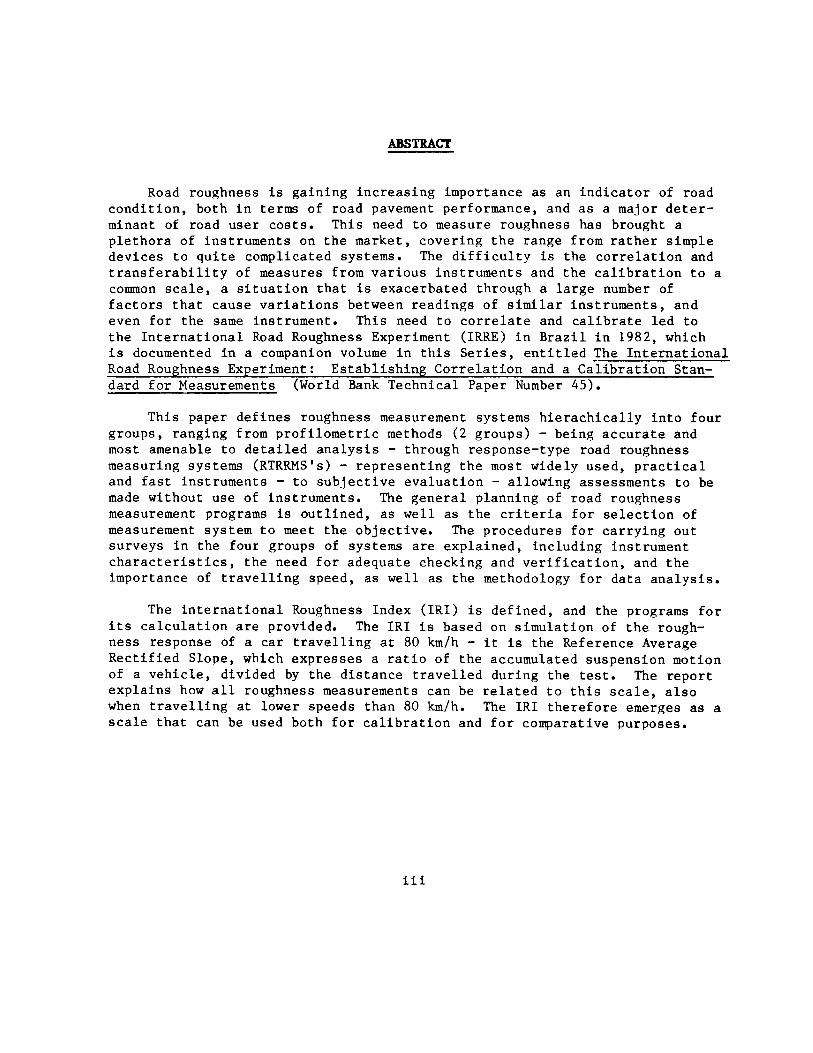
Road roughness is g a i n i n g i n c r e a s i n g importance a s an i n d i c a t o r of road c o n d i t i o n , bo th i n terms of road pavement performance, and a s a major d e t e r - minant of road use r c o s t s . Th i s need t o measure roughness has brought a p l e t h o r a of i n s t r u m e n t s on t h e market , c o v e r i n g t h e range from r a t h e r s imple d e v i c e s t o q u i t e complicated systems. The d i f f i c u l t y i s t h e c o r r e l a t i o n and t r a n s f e r a b i l i t y of measures from v a r i o u s i n s t r u m e n t s and t h e c a l i b r a t i o n t o a common s c a l e , a s i t u a t i o n t h a t i s exacerba ted through a l a r g e number of f a c t o r s t h a t cause v a r i a t i o n s between r e a d i n g s of s i m i l a r i n s t r u m e n t s , and even f o r t h e same ins t rument . Th i s need t o c o r r e l a t e and c a l i b r a t e l e d t o t h e I n t e r n a t i o n a l Road Roughness Experiment (IRRE) i n B r a z i l i n 1982, which i s documented i n a companion volume i n t h i s S e r i e s , e n t i t l e d The I n t e r n a t i o n a l Road Roughness Experiment: E s t a b l i s h i n g C o r r e l a t i o n and a C a l i b r a t i o n Stan- d a r d f o r Measurements (World Bank Technica l Paper Number 45).
T h i s paper d e f i n e s roughness measurement systems h i e r a c h i c a l l y i n t o f o u r groups , r ang ing from p r o f i l o m e t r i c methods ( 2 g roups) - being a c c u r a t e and most amenable t o d e t a i l e d a n a l y s i s - through response-type road roughness measuring systems (RTRRMS1s) - r e p r e s e n t i n g t h e most widely used , p r a c t i c a l and f a s t i n s t r u m e n t s - t o s u b j e c t i v e e v a l u a t i o n - a l lowing assessments t o be made wi thout use of ins t ruments . The g e n e r a l p lann ing of road roughness measurement programs is o u t l i n e d , a s w e l l a s t h e c r i t e r i a f o r s e l e c t i o n of measurement sys tem t o meet t h e o b j e c t i v e . The p rocedures f o r c a r r y i n g o u t s u r v e y s i n t h e four groups of systems a r e e x p l a i n e d , i n c l u d i n g ins t rument c h a r a c t e r i s t i c s , t h e need f o r adequa te checking and v e r i f i c a t i o n , and t h e importance of t r a v e l l i n g speed, a s w e l l a s t h e methodology f o r d a t a a n a l y s i s .
The i n t e r n a t i o n a l Roughness Index ( I R I ) i s d e f i n e d , and t h e programs f o r i t s c a l c u l a t i o n a r e provided. The I R I i s based on s i m u l a t i o n of t h e rough- n e s s response of a c a r t r a v e l l i n g a t 80 km/h - it i s t h e Reference Average R e c t i f i e d S lope , which e x p r e s s e s a r a t i o of t h e accumulated suspens ion motion of a v e h i c l e , d i v i d e d by t h e d i s t a n c e t r a v e l l e d dur ing t h e t e s t . The r e p o r t e x p l a i n s how a l l roughness measurements can be r e l a t e d t o t h i s s c a l e , a l s o when t r a v e l l i n g a t lower speeds t h a n 80 km/h. The I R I t h e r e f o r e emerges a s a s c a l e t h a t can be used bo th f o r c a l i b r a t i o n and f o r comparat ive purposes .
iii
ACKNOWLEDGEMENTS
These g u i d e l i n e s have t h e i r t e c h n i c a l founda t ions i n t h e pub l i shed f i n d i n g s of two major r e s e a r c h p r o j e c t s :
The i n t e r n a t i o n a l Road Roughness Experiment (IRRE) [ I ] , h e l d i n B r a s i l i a i n 1982, and funded by a number of a g e n c i e s , i n c l u d i n g t h e B r a z i l i a n T r a n s p o r t a t i o n P lann ing Company (GEIPOT), The B r a z i l i a n Road Research I n s t i t u t e (IPRIDNER), t h e World Bank (IBRD), t h e French Bridge and Pavement Laboratory (LCPC), and t h e B r i t i s h Transpor t and Road Research Laboratory (TRRL); and
The NCHRP ( N a t i o n a l Coopera t ive Highway Research Program) P r o j e c t 1-18, documented by NCHRP Report No. 228 [ 2 ] .
Per Fossberg (IBRD) and Cesar Queiroz (IPR~DNER) a r e acknowledged f o r t h e i r c o n t r i b u t i o n s i n t h e development of t h e s e g u i d e l i n e s . Also, g r a t e f u l acknowledgement i s extended t o C l e l l H a r r a l (IBRD), who conceived t h e i d e a o f t h e IRRE and a r ranged f o r t h e p a r t i c i p a t i o n of t h e v a r i o u s agenc ies and t h e subsequent p r e p a r a t i o n of t h e s e g u i d e l i n e s .

TABLE OF CONTENTS
CHAPTER 1: SCOPE .......................................................... 1
CHAPTER 2: PLANNING A ROUGHNESS MEASUREMENT PROJECT ....................... 3
......................... 2.1 Overview o f t h e I R I Road Roughness S c a l e 3
2.2 Roughness Measurement Methods ................................... . 6 ................................ 2.2.1 Class 1: P r e c i s i o n p r o f i l e s 6 ....................... 2.2.2 Class 2: Other p r o f i l o m e t r i c methods 7 2.2.3 C1a;ss 3: I R I e s t i m a t e s from c o r r e l a t i o n e q u a t i o n s .......... 8 ...... 2.2.4 Class 4: S u b j e c t i v e r a t i n g s and u n c a l i b r a t e d measures 9
................... 2.3 F a c t o r s A f f e c t i n g Accuracy .................... 1 0 2.3.1 R e p e a t a b i l i t y e r r o r ........................................ 11 2.3.2 C a H b r a t i o n e r r o r .......................................... 12 2.3.3 R e p r o d u c i b i l t y e r r o r ....................................... 13
................................. 2.4 P lann ing t h e Measurement P r o j e c t 14 2.4.1 Long-term network moni to r ing ............................... 14 2.4.2 Short-term p r o j e c t moni to r ing .............................. 15 2.4.3 P r e c i s e moni to r ing f o r r e s e a r c h ............................ 17
CHAPTER 3: MEASUREMENT OR I R I USING PROFILOMETRIC METHODS (CLASSES 1 & 2).19
3.1 D e s c r i p t i o n of Method ............................................ 19
3.2 Accuracy Requirement ............................................. 19
3.3 Measurement of P r o f i l e ........................................... 22 3.3.1 Rod and Level Survey ....................................... 22 3.3.2 TRRL Beam S t a t i c P r o f i l o m e t e r .............................. 26 3.3.3 APL I n e r t i a l P r o f i l o m e t e r .................................. 27 3.3.4 K . J . Law I n e r t i a l P r o f i l o m e t e r s ........................... 29 3.3.5 Other p r o f i l o m e t e r s ........................................ 31
3.4 Computation of I R I ............................................... 31 3.4.1 Equa t ions .................................................. 31 3.4.2 Example program f o r computing I R I .......................... 33 3.4.3 Tables of c o e f f i c i e n t s f o r t h e I R I e q u a t i o n s ............... 35 3.4.4 Program f o r computing c o e f f i c i e n t s f o r t h e I R I e q u a t i o n s ... 35 3.4.5 Tes t i n p u t f o r checking computat ion ........................ 40

CHAPTER 4: ESTIMATION OF I R I USING A CALIBRATED RTRRMS (CLASS 3 ) ........... 45
4.1 S e l e c t i o n and Maintenance of a RTRRMS ............................. 45 4.1.1 The roadmete r ............................................... 45 4.1.2 The v e h i c l e ................................................. 47 ................ 4.1.3 I n s t a l l a t i o n of t h e roadmete r i n t h e v e h i c l e 47 4.1.4 O p e r a t i n g speed .......................................e..... 47 4.1.5 Shock a b s o r b e r s e l e c t i o n .................................... 48 ............................................. 4.1.6 Veh ic le l o a d i n g 49 4.1.7 T i r e p r e s s u r e ............................... ................ 49 4.1.8 Mechanical l i n k a g e s i n t h e roadmeter ........................ 49 4.1.9 T i r e imbalance and out-of-roundness ......................... 49 4.1.10 Temperature e f f e c t s ......................................... 49 ................................. 4.1.11 Water and m o i s t u r e e f f e c t s 50
4.2 C a l i b r a t i o n of a RTRRMS ........................................... 50 4.2.1 C a l i b r a t i o n method .......................................... 51 4.2.2 C a l i b r a t i o n e q u a t i o n ........................................ 53 4.2.3 S e l e c t i o n of c a l i b r a t i o n s i tes ............................. 5 3 ........................ 4.2.4 Determining I R I of c a l i b r a t i o n s i t e s 58 ......................... 4.2.5 Compensation f o r non-s tandard speed 58
4.3 O p e r a t i n g and C o n t r o l T e s t P rocedures ............................. 60 4.3.1 V e h i c l e and roadmete r o p e r a t i o n ............................. 60 4.3.2 Data p r o c e s s i n g .......................................... ..62 4.3.3 Temperature s e n s i t i v i t y t e s t ................................ 63 ..................... 4.3.4 C o n t r o l t e s t s f o r RTRRMS t i m e s t a b i l i t y 63
CHAPTER 5: ESTIE~ATION OF IRI BY SUBJECTIVE EVALUATION (CLASS 4) ............ 71
5.1 D e s c r i p t i v e E v a l u a t i o n Method ..................................... 71 5.1.1 Method ...................................................... 7 1 5.1.2 D e s c r i p t i o n of t h e I R I S c a l e ................................ 71 5.1.3 P e r s o n n e l ................................................... 75 5.1.4 C a l i b r a t i o n ................................................. 75 5.1.5 Survey ...................................................... 75 5.1.6 Data P r o c e s s i n g ............................................. 76
5.2 P a n e l R a t i n g of Ride Q u a l i t y ..................................... 76
REFERENCES.. .............................................................. *87

CHAPTER 1
SCOPE
T h i s document p r e s e n t s g u i d e l i n e s f o r use by personne l i n highway o r g a n i z a t i o n s r e s p o n s i b l e f o r s e t t i n g up o r o p e r a t i n g road roughness moni to r ing programs. It p r o v i d e s guidance on:
* Choosing a method f o r measuring road roughness ;
* C a l i b r a t i n g t h e measurement equipment t o a s t a n d a r d roughness s c a l e ;
* Using p rocedures t h a t e n s u r e r e l i a b l e measurements i n r o u t i n e d a i l y use .
The s u g g e s t i o n s and p rocedures p resen ted h e r e a r e in tended t o gu ide t h e p r a c t i t i o n e r i n a c q u i r i n g road roughness d a t a from which t o b u i l d a roughness d a t a base f o r a road network. Adherence t o t h e s e g u i d e l i n e s w i l l h e l p e n s u r e :
* That t h e roughness d a t a i n d i c a t e road c o n d i t i o n a s i t a f f e c t s u s i n g v e h i c l e s i n terms of r i d e q u a l i t y , u s e r c o s t , and s a f e t y ;
* That d a t a a c q u i r e d i n r o u t i n e measurement o p e r a t i o n s w i l l be r e l a t e d t o a s t a n d a r d roughness s c a l e , and t h a t e r roneous d a t a can be i d e n t i f i e d p r i o r t o e n t r y i n t o t h e d a t a base ;
* That t h e roughness d a t a can be compared d i r e c t l y t o d a t a acqu i red by o t h e r highway o r g a n i z a t i o n s a l s o fo l lowing t h e g u i d e l i n e s ; and
* That t h e roughness measures have t h e same meaning on a l l types of roads used by highway t r u c k s and passenger c a r s , i n c l u d i n g a s p h a l t , c o n c r e t e , s u r f a c e t r e a t m e n t , g r a v e l , and e a r t h s u r f a c e s .
The p rocedures p r e s e n t e d i n t h i s document a r e p r i m a r i l y a p p l i c a b l e t o roughness measurements of two t y p e s :
* D i r e c t measurement of roughness on t h e s t a n d a r d s c a l e , d e r i v e d from t h e l o n g i t u d i n a l p r o f i l e of t h e road
* E s t i m a t i o n of t h e s t a n d a r d roughness measure, u s i n g c a l i b r a t e d response-type road roughness measurement systems (RTRRMSs)


CHAPTER 2
PLANNING A ROUGHNESS MEASUREMENT PROJECT
- - The design of a p ro j ec t f o r surveying the roughness of a road
network should s t a r t wi th a c l e a r understanding of t he ob jec t ives t o be achieved from the measurement e f f o r t . A s u b s t a n t i a l investment of manpower and money can be consumed i n a t y p i c a l p r o j e c t , thus i t i s d e s i r a b l e t o design the program ca re fu l ly . The design i t s e l f i s a syn thes i s process taking i n t o account the p ro j ec t goa l s , the resources a v a i l a b l e , and the environment of the pro jec t . Perhaps the most c r i t i c a l element i n the design i s the s e l e c t i o n of a roughness measurement method t h a t i s p r a c t i c a b l e , y e t s u i t a b l y accura te f o r the purposes of t he pro jec t . This s ec t ion reviews the var ious measurement methods a v a i l a b l e , c l a s s i f i e d according t o how d i r e c t l y they measure roughness on a s tandard s c a l e (General ly , t he more d i r e c t methods a r e a l s o the most accura te ) . I n add i t i on , i t expla ins the types of e r r o r s t o be a n t i c i p a t e d , and t h e i r importance t o var ious kinds of measurement p ro j ec t s .
2.1 Overview of the I R I R o a d R o u g h n e s s Scale
I n order t o address s p e c i f i c s of roughness measurement, o r i s s u e s of accuracy, i t i s f i r s t necessary t o de f ine t h e roughness s ca l e . I n t he i n t e r e s t of encouraging use of a common roughness measure i n a l l s i g n i f i c a n t p r o j e c t s throughout the world, an I n t e r n a t i o n a l Roughness Index ( IRI ) has been se lec ted . The I R I i s so-named because i t was a product of t he I n t e r n a t i o n a l Road Roughness Experiment (IRRE), conducted by research teams from B r a z i l , England, France, the United S t a t e s , and Belgium f o r t he purpose of i den t i fy ing such an index. The IRRE was held i n B r a s i l i a , Braz i l i n 1982 [ l ] and involved the con t ro l l ed measurement of road roughness f o r a number of roads under a v a r i e t y of condi t ions and by a v a r i e t y of instruments and methods. The roughness s c a l e s e l e c t e d a s the I R I was t h e one t h a t bes t s a t i s f i e d the c r i t e r i a of being t ime-stable , t r a n s p o r t a b l e , and r e l e v a n t , while a l s o being r e a d i l y measurable by a l l p r a c t i t i o n e r s
The I R I i s a s tandardized roughness measurement r e l a t e d t o those obtained by response-type road roughness measurement systems (RTRRMs), wi th recommended u n i t s : meters per ki lometer (mlkm) = mil l ime te r s per meter (mm/m) = s lope x 1000. The measure obtained from a RTRRMS i s c a l l e d e i t h e r by i t s t echn ica l name of average r e c t i f i e d s lope (ARS), o r more commonly, by the u n i t s used (mmlkm, in/mi, e tc . ) . The ARS measure i s a r a t i o of t he accumulated suspension motion of a veh ic l e ( i n , mm, e t c . ) , divided by the d i s t ance t r a v e l l e d by the veh ic l e during the t e s t (mi, km, e t c . ) . The re ference RTRRMS used f o r the I R I i s a mathematical model, r a t h e r than a mechanical system, and e x i s t s a s a computation

procedure applied to a measured profile. The computation procedure is called a quarter-car simulation (QCS), because the mathematical model represents a RTRRMS having a single wheel, such as the BI Trailer and BPR Roughometer. When obtained from the reference simulation, the measure is called reference ARS (RARs). This type of measure varies with the speed of the vehicle, and therefore, a standard speed of 80 km/h is specified in the definition of the IRI. Thus, the more technical name for the IRI is RARS80, indicating a measure of average rectified slope (ARS) from a reference (R) instrument at a speed of 80 km/h.
The mathematical vehicle model used to define the IRI is the same as that described in the 1981 NCHRP Report 228 [2], with the single difference that the IRI is computed independently for each wheeltrack. wh he model in NCHRP Report 228 was computed for two wheeltracks simultaneously, thus replicating the performance of a RTRRMS based on a passenger car, or a two-wheel trailer.) The IRI version is more transportable, and was demonstrated as yielding RTRRMS accuracy just as high as the NCHRP version for all types of RTRRMSs.
The IRI is defined as a characteristic of the longitudinal profile of a travelled wheeltrack, rather than as a characteristic of a piece of hardware, in order to ensure time stability, Thus, direct measurement of the IRI requires that the profile of the wheeltrack be obtained.
The particular profile characteristic that defines the IRI was demonstrated to be directly measurable by most profilometric methods (more than any of the other profile-based roughness numerics that were considered in the IRRE). At the same time, the IRI profile characteristic is so highly compatible with the measures obtained by RTRRMSs that these instruments can be calibrated to the IRI scale to achieve the best (or close to the best) accuracy that is possible with this type of instrument, The IRI is also strongly related to the subjective opinions about road roughness that can be obtained from the public. Because the IRI is (1) measurable by many profilometric methods, (2) highly correlated with the measures from RTRRMSs, and (3) highly correlated with subjective opinion, it is a highly transportable scale.
Figure 1 shows the approximate range of IRI roughness on different types of roads.
It should be recognized that the IRI is a numeric that summarizes the roughness qualities impacting on vehicle response, but which may not be the most appropriate for other applications. More specifically, the IRI is appropriate when a roughness measure is desired that relates to:
* overall vehicle operating cost

IRI (m/km = mm/m)
16 EROSION GULLEYS AND DEEP DEPRESSIONS
14
12 FREQUENT SHALLOW DEPRESSIONS, SOME
10
8
6
4
2
0
O= ABSOLUTE PERFECTION
NORMAL USE
Fig. 1. The IRI roughness scale.

* o v e r a l l r i d e q u a l i t y
* dynamic wheel loads (damage t o the road from heavy t rucks ; braking and cornering s a f e t y l i m i t s a v a i l a b l e t o passenger c a r s )
* o v e r a l l su r f ace condi t ion
The I R I i s a l s o recommended whenever the measurements w i l l be obtained using a RTRRMS a t highway speeds (50 - 100 km/h), regard less of the use made of the data .
However, when p ro f i l ome t r i c methods a r e used t o measure wheeltrack roughness, then o the r measures may serve a s b e t t e r i n d i c a t o r s f o r some q u a l i t i e s of pavement condi t ion , o r f o r s p e c i f i c components of vehic le response encompassed by the I R I . These gu ide l ines address only the measurement and es t imat ion of the I R I .
2.2 Roughness Measurement Methods
The many approaches f o r measuring road roughness i n use throughout t he world can be grouped i n t o four gene r i c c l a s s e s on the b a s i s of how d i r e c t l y t h e i r measures p e r t a i n t o the I R I , which i n t u r n a f f e c t s the c a l i b r a t i o n requirements and the accuracy assoc ia ted with t h e i r use.
2.2.1 Class 1: Precision profiles. This c l a s s r ep re sen t s the h ighes t s tandards of accuracy f o r measurement of I R I . A Class 1 method r equ i r e s t h a t the long i tud ina l p r o f i l e of a wheeltrack be measured ( a s a s e r i e s of accura te e l e v a t i o n po in t s closely-spaced along the t r a v e l l e d wheelpath) a s a b a s i s f o r c a l c u l a t i n g the I R I value. For s t a t i c p ro f i l ome t r i c methods, the d i s t ance between samples should be no g r e a t e r than 250 mm ( 4 measures/meter) and the p rec i s ion i n the e l eva t ion measures must be 0.5 mm f o r very smooth pavements. ( ~ e s s p rec i se measurements a r e acceptable f o r rougher su r f aces , a s spec i f i ed i n Sect ion 3.2.) High-speed prof i lometers o f f e r a p o t e n t i a l means f o r measuring I R I qu ick ly ; however, the prof i lometer must be va l ida t ed a t some time aga ins t an e s t ab l i shed procedure such a s rod and l e v e l t o prove i t s accuracy. A t t he present t ime, only rod and l e v e l (Sect ion 3.3.1) and the TRRL Beam ( s e c t i o n 3.3.2) methods have been demonstrated t o be v a l i d Class 1 methods f o r determining I R I over a broad range of roughness l e v e l s and road types f o r the 320 m s i t e l eng th used i n the IRRE .
Methods i n t h i s c l a s s a r e those t h a t produce measures of such high q u a l i t y t h a t r e p r o d u c i b i l i t y of the I R I numeric could not be improved. While t h i s d e f i n i t i o n might a t f i r s t appear t o imply an unreachable i d e a l , t he re i s usua l ly a p r a c t i c a l l i m i t t o the r e p e a t a b i l i t y t h a t can be obtained i n measuring road roughness, even with a "per fec t" method and/or instrument. The p r a c t i c a l l i m i t r e s u l t s from the i n a b i l i t y t o

measure roughness repea ted ly i n exac t ly the same wheeltrack. Therefore, a method q u a l i f i e s a s Class 1 i f measurement e r r o r i s n e g l i g i b l e i n comparison with the unce r t a in ty a s soc i a t ed wi th t r y i n g t o l o c a t e exac t ly the same wheel t rack twice.
I n the IRRE t he methods found t o q u a l i f y a s Class 1 had n e g l i g i b l e measurement e r r o r f o r s i t e s 320 m long, when the wheel t racks were marked wi th painted re ference spo t s spaced a t about 20 m i n t e r v a l s . The r e p e a t a b i l i t y under these condi t ions i s about 0.3 m/km I R I on paved roads, and about 0.5 m/km f o r a l l o t h e r road types. For wheelpaths marked even more p r e c i s e l y , methods descr ibed i n these gu ide l ines a s Class 1 could perhaps not q u a l i f y a s Class 1 (al though i t i s uncommon t o have an a p p l i c a t i o n where such a high l e v e l of accuracy i s needed). On the o the r hand, l e s s s t r i n g e n t s p e c i f i c a t i o n s might be s u i t a b l e i f longer t e s t s i t e s were used, o r i f the wheeltracks were not marked a t a l l .
I n many cases , a method t h a t y i e l d s t h i s l e v e l of accuracy w i l l have an a s soc i a t ed disadvantage of r equ i r ing a g r e a t d e a l of e f f o r t t o make the roughness measurement ( f o r example, by the rod and l e v e l method). The accuracy obtained using a Class 1 method by d e f i n i t i o n matches o r exceeds the requirements of a given a p p l i c a t i o n , and thus the Class 1 method i s viewed a s having primary u t i l i t y f o r v a l i d a t i n g o t h e r methods, o r when s p e c i a l high-accuracy da t a a r e required.
2.2.2 Class 2: Other profilometric rethods. This c l a s s inc ludes a l l o the r methods i n which p r o f i l e i s measured a s the b a s i s f o r d i r e c t computation of the I R I , but which a r e not capable of the accuracy required f o r a Class 1 measurement. Though the hardware and methods used f o r p r o f i l e measurement a r e f u n c t i o n a l l y v e r i f i e d by an independent c a l i b r a t i o n process , they a r e l imi t ed t o accuracy o r bandwidth l e s s than t h a t needed t o q u a l i f y a s a Class 1 method. Consequently, the I R I value computed from a Class 2 p r o f i l e measurement may not be accura te t o the p r a c t i c a l l i m i t due t o random o r b i a s e r r o r s over some range of condit ions. This c l a s s p re sen t ly inc ludes I R I va lues computed from p r o f i l e s measured with high-speed prof i lometers and with s t a t i c methods t h a t do not s a t i s f y the p rec i s ion and/or measurement i n t e r v a l requirements s p e c i f i e d i n Sect ion 3.2.
A t t he present t ime, t he APL T r a i l e r ( s e c t i o n 3.3.3) i s the only dynamic prof i lometer t h a t has been experimental ly va l ida ted over t he range of roughness covered i n the IRRE. The GMR-type I n e r t i a l Prof i lometer with fol lower wheels has been va l ida t ed f o r roads with roughness l e v e l s l e s s than an I R I va lue of about 3 m/km [ 2 ] , above which e r r o r s a r e introduced due t o bounce of the fol lower wheels. This type of design i s no longer commercially a v a i l a b l e i n the United S t a t e s , however, a s the fol lower wheels have been replaced with non-contacting sensors t o el imin 'a te the bounce problem. Two high-speed prof i lometers

are presently sold by K.J. Law, Inc. (section 3.3.4), and both are designed to provide the IRI roughness during measurement. Both are considered as Class 2 systems at this time, although their accuracy and range of operation have not been verified against rod and level yet. Tests with these and other profilometers have been performed, but the analyses of the data have not yet been completed sufficiently to
1 quantify their ability to measure IRI . High-speed profilometers have the disadvantage of being the most
expensive and complex instrumentation systems used to measure road roughness, and generally require operators with engineering training. Yet, they offer a great advantage in being able to obtain high-quality measurements rapidly, without requiring that great effort be spent in maintaining calibration. Detailed procedures for operating a profilometer to measure IRI are highly specific to the design of the profilometer; hence, the manufacturer should be consulted. Sections 3.3.3 and 3.3.4 briefly describe several of the high-speed profilometers that have been used to measure IRI.
2.2.3 Class 3: IRI estimates from correlation equations. By far, the majority of road roughness data that is collected throughout the world today is obtained with RTRRMSs. The RTRRMS measure depends on the dynamics of a vehicle to scale the measurements to yield roughness properties comparable to the IRI. The dynamic properties are unique for each vehicle, however, and change with time, Thus, the "raw" measures of ARS obtained from the RTRRMS must be corrected to the IRI scale using a calibration equation that is obtained experimentally for that specific RTRRMS. Because the dynamics of a vehicle change easily, very rigorous maintenance and operating procedures must be employed for the vehicles used, and control testing must be made a routine part of normal operations. When changes occur, there is no simple correction that can be applied; instead, the entire roadmeter-vehicle system must be re- calibrated.
This class also includes other roughness measuring instruments capable of generating a roughness numeric reasonably correlated to the IRI (e.g., a rolling straightedge). The measures obtained can be used to estimate IRI through regression equations if a correlation experiment is performed. This approach is usually more trouble than it's worth
'1n 1984 a Road Profilometer Meeting was held in Ann Arbor, Michigan, to determine the performance characteristics of a number of profilometers, including both of the current non-contacting systems from K.J.Law, Inc. (USA), the Swedish VTI laser system, the APL Trailer, and several non-commercial systems. The study, which was funded by the U.S. Federal Highway Administration (FHWA) and conducted by UMTRI, is still underway [ 3 I .

(better measures can be obtained with less effort), unless there is a need to convert a large amount of past data to the IRI scale.
A method for measuring roughness qualifies as Class 3 if it uses the "calibration by correlation" approach described in Section 4.2, regardless of what type of instrumentation or vehicle is used to obtain the uncorrected roughness measure. While most Class 3 methods will employ a roadmeter that accumulates suspension motion to measure ARS as described in Section 4.1, other systems are in use that employ accelerometers or other types of instrumentation. However, the roadmeter-based RTRRMS that measures ARS most closely matches the IRI concept, and these guidelines concentrate on the calibrated RTRRMS as the principle Class 3 method.
Unless a RTRRMS is calibrated by correlation, it does not qualify as a Class 3 method. Without the calibration, there is no verifiable link between the measures obtained with any two RTRRMSs, nor to the IRI scale.
The reproducibility associated with a calibrated RTRRMS is about 0.5 m/km (14%) for paved roads for sections 320 m long, and about 1.0 m/km (18%) for unpaved surfaces of that length. These accuracy figures are only approximate averages, as the errors generally vary both with roughness and surface type. Better accuracy is possible by using longer test sections.
2.2.4 Class 4: Subjective ratings and uncalibrated reasures. There are situations in which a roughness data base is needed, but high accuracy is not essential, or cannot be afforded. Still, it is desirable to relate the measures to the IRI scale. In those cases, a subjective evaluation involving either a ride experience on the road or a visual inspection could be used. Another possibility is to use the measurements from an uncalibrated instrument. Conversion of these observations to the IRI scale is limited to an approximate equivalence, which can best be established by comparison to verbal and/or pictorial descriptions of roads identified with their associated IRI values, as described in Section 5.0. Essentially, the estimates of equivalence are the calibration, however approximate, and they may be considered to be "calibration by d.escription."
When these subjective estimates of roughness are converted to the IRI scale the resolution is limited to about six levels of roughness with accuracy ranging from 2 - 6 m/km (about 35%) on the IRI scale. (~oughness accuracy, expressed either in absolute units of m/km or as a percentage, will generally vary with roughness level and surface type.)
Note that unless a valid calibration by correlation is used with a RTRRMS, there is no way to link the measure to the standard scale. Thus, an uncalibrated RTRRMS falls within Class 4.
2.3 Factors Affecting Accuracy
Roughness data are normally utilized in applications representing two extremes: (1) statistical analyses involving roughness measurements on major segments of a road network, and (2) individual studies related to roughness at specific road sites. The roughness data will necessarily include some errors arising from random and systematic effects. The significance of these errors depends on the nature of the application for which the data are intended.
An example of the first type of application is a road-user cost study, in which the data base of operating costs for a fleet of vehicles is regressed against the data base of roughness for the roads on which those vehicles were operated. In that case, the need is to determine levels of roughness for comparison with trends of costs, using regression methods. Random errors in individual roughness measurements, caused by poor precision or a peculiar road characteristic, will tend to average out if the study includes a large number of road sites. Thus, random error is not of great concern for this type of study. On the other hand, systematic errors will bias the cost relationships obtained. Therefore, steps should be taken to keep the systematic errors to minimal levels. The results of the study will not be transportable unless a standard roughness scale is used, and steps are taken to ensure that the roughness data more or less adhere to that scale.
Studies that involve monitoring roadway deterioration or the effects of maintenance are examples of the second type of application. In these cases, it is of interest to maintain a continuing record of small changes in the roughness condition at specific road sites. Random errors in measurement will reduce the certainty with which the trends of interest can be discerned. A constant bias in the data can be determined and corrected in order to compare roads or apply economic criteria, but it is perhaps even more critical to ensure that the bias does not change with time. Thus, for measurements to be used for these applications, the practitioner should employ procedures that will minimize random errors while also maximizing time-stability. This normally translates into using the same equipment and personnel for regular monitoring of a road site, utilizing repeat tests to improve repeatability, and carefully maintaining the calibration of the equipment.
The end use of the roughness data in applications such as these has a direct impact on the accuracy that will be necessary in the

measurement procedures. In turn, the accuracy determines how much effort must be devoted to obtaining good data. Each application will have peculiar sensitivity to different error sources. In order to make rational decisions about the quality of the measurements to be obtained, it is helpful to realize that inaccuracy in roughness measurements will arise from three types of error sources.
2.3.1 Repeatability error. When repeated measurements are made with an instrument, exact agreement cannot be expected because the measurement process includes random effects that vary from measurement to measurement. The level of repeatability may not always be evident, because instruments often involve a quantization of the output that masks the effects of small variations. In these cases, the repeatability should be assumed to be no better than at least half the quaatization size. For example, an RTRRMS that produces counts corresponding to 3.0 mm has a repeatability error of at least 1.5 mm.
When measuring road roughness by carefully surveying the longitudinal profile, the precision is limited by: (1) the instrumentation used to measure the profile, (2) the random locations of the specific points along the wheeltrack where the elevation measures are taken, and (3) the partly-random selection of the lateral position of a traveled wheeltrack. The first two errors are reduced oy specifying higher quality profile measurements (i.e., more accurate elevation measurements and more closely spaced survey points). When these error sources are controlled, then the imprecision associated with identifying the wheeltrack location becomes the most significant factor, accounting for variations up to 5% when the wheeltrack length is 320 mer
When measuring roughness with a RTRRMS, repeatability is affected by the partly-random variation in lateral position of the RTRRMS on the road, and also by other random factors such as variations in its operating speed and small changes in the vehicle dynamics that occur even over a short time. These sources of variability can be kept to the same level as for direct profile measurement with careful operation.
Repeatability errors are basically random in nature, and can thus be controlled by extending the measurement process so that the random errors cancel out due to averaging. This can be accomplished most simply by using test sections of sufficient length,
A second form of averaging is obtained by making repeated measurements on the same test site. In this way, repeatability error can be reduced on shorter sections that are not long enough for sufficient averaging. In general, the repeatability error is inversely prop~rtional to the square root of the total length covered, where the total length is the site length times the number of repeat measurements. Thus, the error e:spected on a 1.6 km test site is approximately the same

a s would be obtained on a 320 m t e s t s i t e a f t e r f i v e r epea t s ( 5 x 320 m = 1.6 km). A s a r u l e of thumb, a t o t a l l eng th of 1.6 km (1.0 mi le ) o r longer i s recommended t o minimize r e p e a t a b i l i t y e r r o r f o r instruments used a t highway speeds.
Another means f o r increas ing the averaging f o r a RTRRMS instrument i s t o use a lower speed f o r a given l eng th of t e s t s i t e ; however, t h i s approach i s not recommended, because changing the speed a l s o changes the meaning of the roughness measure f o r the RTRRMS and inc reases o t h e r e r r o r s .
2.3.2 Calibration error. Systematic e r r o r s e x i s t i n instruments. These cause the measurements of one t o be c o n s i s t e n t l y d i f f e r e n t from those of another , o r cause one instrument t o vary with time. This can be cor rec ted by c a l i b r a t i o n , so t h a t the roughness measurements a r e resca led t o cancel sys temat ic d i f f e r e n c e s br inging the measures t o a common sca le . However, i f the c a l i b r a t i o n does not cover a l l of the v a r i a b l e s t h a t a f f e c t the measurement, then the r e sca l ing may not be c o r r e c t , and a c a l i b r a t i o n e r r o r remains.
Profilometric methods (Classes 1 and 2): Cal ib ra t ion e r r o r i s minimal when d i r e c t p r o f i l e measurements a r e used t o ob ta in the I R I . The instruments t h a t measure the p r o f i l e a r e c a l i b r a t e d a t the f a c t o r y , and do not change much when given reasonable care . Nonetheless, sys temat ic e r r o r s can appear i n profi le-based measures when (1) t h e p r o f i l e e l eva t ion measures conta in e r r o r s (u sua l ly making the p r o f i l e seem rougher than i t i s ) , ( 2 ) when p r o f i l e measures a r e spaced too f a r a p a r t such t h a t some of the roughness f e a t u r e s a r e missed (making . the p r o f i l e seem smoother), and (3 ) when p r o f i l e measures a r e subjected t o a smoothing o r a waveband l i m i t a t i o n a s occurs with a dynamic prof i lometer (making the p r o f i l e seem smoother). The s p e c i f i c a t i o n s and procedures recommended i n Sec t ions 3.2 and 3.3 were designed t o hold these e f f e c t s t o n e g l i g i b l e l eve l s .
RTRRMSs (Class 3): Cal ib ra t ion by c o r r e l a t i o n with a re ference (Sec t ion 4.2) i s required f o r a RTRRMS f o r many reasons, inc luding these important th ree :
1 ) The o v e r a l l dynamic response of any p a r t i c u l a r RTRRMS veh ic l e w i l l d i f f e r t o some degree from t h a t of the reference. This e f f e c t can cause the "raw" ARS measure from the RTRRMS t o be higher o r lower than corresponding I R I va lues , depending on whether the RTRRMS i s more o r l e s s responsive than the reference.
2) The roadmeter i n the RTRRMS gene ra l ly has f r eep lay and o the r forms of h y s t e r e s i s t h a t cause i t t o miss counts , r e s u l t i n g i n lower roughness measures.

3) The RTRRMS suspension motions inc lude e f f e c t s from f a c t o r s o t h e r than road roughness, such a s t i r e out-of-roundness. This induces h igher roughness measures.
The sys temat ic e r r o r sources i n a RTRRMS i n t e r a c t , and a r e nonl inear . Their e f f e c t can change with roughness, sur face type , temperature, and o the r environmental f a c t o r s . The only way they can be taken i n t o account i s through c o r r e l a t i o n with measures of I R I obtained wi th a re ference method (Class 1 o r 2 ) . This opera t ion i s e s s e n t i a l l y a " c a l i b r a t i o n by co r re l a t ion . " The procedure descr ibed i n Sec t ion 4.2 i s designed t o e l imina te c a l i b r a t i o n e r r o r from RTRRMS measurements.
2.3.3 Reproducibility error. When measuring a complex q u a l i t y such a s road roughness with a method o the r than d i r e c t p r o f i l e measurement, i t i s poss ib l e (and common) f o r two d i f f e r e n t instruments t o rank seve ra l roads i n a d i f f e r e n t order by roughness. An e r r o r e x i s t s t h a t i s random with road s e l e c t i o n , but i s sys temat ic f o r the instrument. Even though the measures obtained with one instrument ( o r method) may be h ighly r epea t ab le , they a r e not reproduced when measures a r e obtained using a d i f f e r e n t instrument. The problem i s t h a t t he two measuring methods have d i f f e r e n c e s t h a t a r e more complex than simple s c a l e f a c t o r s . While r e p e a t a b i l i t y e r r o r s can be con t ro l l ed using repeated t e s t s and averaging, and c a l i b r a t i o n e r r o r s can be con t ro l l ed by v a l i d c a l i b r a t i o n methods, r e p r o d u c i b i l i t y e r r o r s w i l l always e x i s t when the measuring instrument d i f f e r s from the reference.
When measures a r e obtained from Class 1 p r o f i l e measurement, r e p r o d u c i b i l i t y e r r o r from the instrument i s e s s e n t i a l l y non-exis tent , a
and unce r t a in ty e x i s t s only because of the r e p e a t a b i l i t y l i n i t s . Repea tab i l i t y c o n t r o l s can the re fo re be used t o improve the o v e r a l l accuracy.
But when measures a r e obtained from a RTRRMS, the re i s no method of t e s t design o r d a t a processing t h a t can reso lve the d i f f e r ences among instruments t h a t causes one t o measure high on one road and low on another , r e l a t i v e t o the I R I . What can be done, however, i s t o adopt a procedure t h a t matches the c h a r a c t e r i s t i c s of the RTRRMS t o the re ference t o the c l o s e s t degree possible . The gu ide l ines f o r s e l e c t i n g and opera t ing a RTRRMS ( s e c t i o n s 4.1 and 4.3) were w r i t t e n with t h i s i n mind.
Another s t e p t h a t can be taken f o r any measurement method i s t o measure roughness f o r longer road s i t e s . Since the r e p r o d u c i b i l i t y e r r o r i s random f o r each road s e c t i o n , i t can be reduced somewhat through the averaging t h a t occurs when longer road s i t e s a r e used. Unlike t h e r e p e a t a b i l i t y e r r o r , t h i s e r r o r does not neces sa r i l y decrease wi th the square root of length.

Reproducibility is not improved by repeating measures on the same site, since the effect is systematic for that site.
2.4 Planning the Measurement Project
The execution of a high-quality road-zoughness measuring program is critically dependent on establishing well-thought-out procedures that are adhered to in a strict and consistent fashion throughout the project. This section outlines the planning needs for the three main kinds of roughness measurement projects, to aid the planner in appreciating the logistics that are involved.
2-4.1 Long-term network monitoring. Long-term roughness monitoring programs are an integral part of network condition evaluation surveys and pavement management systems. Typical objectives include:
1) Summary of network condition on a regular basis for evaluation of policy effectiveness
2) Input into a network-level economic analysis of pavement design standards, maintenance policy, and transportation costs
3) Quantifying project condition for prioritizing maintenance and rehabilitation programs.
To meet these objectives, the measurements will usually be continuous over links of the network and the total length will exceed 1000 km (or even 10,000 km). It is essential that measures made in different 'areas of the network be directly comparable, and that the measures be consistent over time. However, the accuracy requirements for individual roughness measurements will generally not be as demanding as for other types of projects, because data averaging will reduce the effects of random errors. Of the three sources of error described in Section 2.3, the calibration error is the most critical to control.
When planning a long-term monitoring program, one should consider:
a) Type of roughness measuring instruments: The rapid collection and automatic processing of data are paramount considerations to facilitate storage in a data bank, and streamline analysis. Only instruments that can be operated at the higher speeds should be considered. he instrument should operate at least at a speed of 50 km/h, and preferably at 80 km/h or faster.) Any type of RTRRMS is suitable. A high-speed profilometer is also suitable and can provide useful descriptive numerics in addition to IRI.
b) Number of instruments: When the network is very large or spread-out, more than one instrument may be required. If this is the

case, a fleet of RTRRMSs might be more affordable than a fleet of profilometers. The vehicles used for RTRRMSs preferably should be of the same make for the sake of interchangeability, although this is not essential when sound calibration procedures are followed.
2 c) Calibration sections (for RTRRMSs only ): A series of eight to
twenty calibration sections will be needed at a central location and possibly at distant regional locations to permit full calibration of the test vehicles at regular intervals (section 4.2).
d) Control. sections: A small number of control sections (three to five) will be needed in every region where the instruments will operate to permit control checks on a daily or weekly basis (section 4.3.4).
3 e) Measurement speed (for RTRRMSs only ): This may be a compromise of conflicting considerations. The standard speed of 80 km/h is likely to be applicable in the majority of situations. Severe road geometry or congestion will dictate a lower speed of 50 or 32 km/h on some links, but this should not influence the choice for the majority of the survey. The simultaneous collection of other data during the survey may influence the choice.
" - f) Data processing and reporting: Data collection must include
location and other event markers for reconciliation with other pavement management data. Computerization at the earliest possible stage and use of standard coding forms where necessary should be considered to facilitate data entry. Measurements should be recorded at intervals of no more than 1 k.m. Reporting will usually comprise mean values either by link or homog:eneous section of 10 km or longer, with summary histograms of roughness distribution by road length. These reporting units should coincide with at least the major changes in traffic volumes to facilitate estimates of vehicle operating costs. For efficiency, the data can be managed so as to permit separating the more detailed reporting requirements of simultaneous project evaluation and prioritization studies.
2.4.2 Short-term project monitoring. Evaluation of specific rehabilitation or betterment projects involves either short-term observations over periods up to 3 years or one-shot roughness measurements. T'ypically, the sites will range from 5 to 50 km in length and will not necessarily be contiguous. Careful consideration should be given to the detail and accuracy required, as accuracy requirements can sometimes be more stringent than for long-term network monitoring
'~rofilometers are calibrated at the factory or in a laboratory.
'speed requirements for prof ilometers are specific to the prof ilometor design.

(Section 2.4.1). On the other hand, if only approximate roughness measures are needed, considerable economy can be achieved.
If a history of surface roughness is desired, then the instrument should be capable of providing repeatable measures over a period of time, and it will be important to maintain calibration error to small levels. Also, if high accuracy is desired, repeated measurements can be averaged to reduce the repeatability error that might otherwise mask small changes in roughness. In general, efficiency in data acquisition is not critical for short-term projects, and therefore emphasis should be placed on obtaining data with quality as high as possible from the instrumentation.
In some cases, transportability of the data (obtained by using the standard IRI scale) may not be as critical as maintaining a high standard of internal consistency. In practice, however, the careful controls needed to maintain internal consistency will often result in adherence to the IRI scale anyway (particularly for RTRRMSs).
a) Profilometric Methods (Classes 1 and 2): Profilometric methods are suitable and can optionally provide useful descriptive numerics in addition to IRI, which can be used to diagnose the nature and probable sources of distress. or example, the APL 72 system normally provides three waveband roughness indices. The predominantly long wavelength roughness indicates subgrade or foundation instability, whereas short wavelength roughness indicates base or surfacing distress.)
If a profilometer is available, it can probably be applied with little modification in procedure, requiring only a more detailed reporting format and possibly more careful marking of test sites. If no roughness measuring instrumentation is available, a profilometer might be imported temporarily with less overall cost than the purchase of less sophisticated systems that require extensive calibration effort.
b) Calibrated RTRRU (Class 3): These methods need to be under rigorous control to be satisfactory when high accuracy is desired. If possible, a single instrument should be used to perform all of the measurements in order to minimize reproducibility error. The complete calibration (see Section 4.2) may need to be repeated more frequently than for other applications, as even small changes in the response properties of the RTRRMS may mask the desired roughness information.
If a fully equipped RTRRMS is available (from a long-term project), it can possibly be applied with little modification in procedure, requiring only more detailed measurement and reporting formats. However, if the accuracy requirements are significantly more stringent than for the other project, then the procedures will need to
be modified accordingly by controlling the vehicle condition more carefully (section 4.1) and by applying calibrations more frequently (section 4.2). If the primary calibration sites for the test vehicle are distant (over 100 km) from the project, a series of three to six control sites should be established nearby (Section 4.3.4).
If measures from one RTRRMS are to be compared for different sites, it is absolutely essential that all of the measurements be made at the same speed. If it is not possible to perform measures at 80 km/h, then the highest speed that can be used at all sites should be chosen. In selecting a non-standard speed, the reproducibility error may be worse for comparing data from different RTRRMSs, but it will be better for comparing data obtained with the single RTRRMS used in the study. Thus, the data will be internally more consistent, at the expense of transportability.
If a system has to be set up for the project, minimum requirements can be established suiting either an imported temporary system or the beginnings of a system that might later be expanded.
c) Uncalibrated measures or subjective ratings (Class 4): If low accuracy and precision are acceptable, as often applies in the early stage of a project or in areas of poor access, a RTRRMS with approximate calibration or a subjective evaluation method (Class 4) can be used quickly with high utility and low set-up costs.
d) Data processing and reporting: Readings should usually be taken at 0.1 or 0.2 km intervals. Reporting will usually include longitudinal-profile bar graphs with 95th percentile values and means over homogeneous lengths, or a coding that highlights critical sections. The presentation should aid the prioritization, planning, and design of rehabilitation and betterment projects.
2.4.3 Precise monitoring for research. Research studies which aim to quantify relatively small changes in roughness of roads over short- to medium-term periods of three to six years require a high accuracy and precision of measurement, Many such studies are being instituted in countries seeking to calibrate or establish road deterioration predictive functions for use in pavement management and economic evaluation analyses. Usually the sections are short, of 1 km length or less, and may be widely scattered throughout a region and between regions in order to meet experimental design requirements of traffic, pavement, and climate permutations.
Where such studies involve short road sections, preference should be given to profilometric methods (Classes 1 and 2), including static methods (e.g., rod and level) if a high-speed profilometer is not available or is not sufficiently accurate. RTRRMS Class 3 methods have

o f t e n been used f o r t h i s a p p l i c a t i o n , but gene ra l l y l ack adequate p r e c i s i o n and g ive r i s e t o u n c e r t a i n t y i n t h e t rend da ta . It should be noted t h a t p r o f i l e measures can a l s o be processed t o y i e l d a v a r i e t y of su r f ace cond i t i on i n d i c a t o r s o the r than the I R I , whereas RTRRMSs a r e capable of only t he s i n g l e type of measurement.
A trade-off on t he frequency of measurement i s poss ib l e : Class 1 o r 2 measures need be made only annual ly and i n conjunct ion wi th major maintenance a c t i v i t i e s , because of t h e i r h igher accuracy. However, Class 3 RTRRMS measures should be made a t l e a s t two t o t h r e e t imes per y e a r , i n o rde r t o ensure confidence i n t h e d a t a t rends. P o r t a b i l i t y of t h e system i s important : Class 3 methods r equ i r e t he es tab l i shment of support ing c o n t r o l s e c t i o n s i n d i s t a n t reg ions , whereas Class 1 o r 2 systems do not.
Data processing and a n a l y t i c a l methods w i l l u sua l ly be p ro j ec t - s p e c i f i c ; t h u s , t he se t o p i c s a r e no t addressed here. Reporting should inc lude computation of t h e I R I f o r t h e purposes of t r a n s f e r a b i l i t y , even i f o t h e r numerics a r e used more d i r e c t l y i n t h e research.

CHAPTER 3
WEBSURKMENT OF IlU USING PROPILOMETRIC METBODS (CUSSES 1 & 2)
3.1 Description of Method
Class 1 and 2 measurements of the IRI can only be obtained from a longitudinal profile of a road. A longitudinal profile is a vertical section along the wheeltrack, which indicates the elevation of the surface as a fun.ction of longitudinal distance. The profile is described by the set of elevation values, spaced at close intervals along the wheeltrack. In order to summarize the hundreds or thousands of numbers that constitute a profile, an analysis procedure is performed that calculates the IRI as a single statistic quantifying the roughness. The calculations are usually performed using some form of digital computer. A programmable pocket calculator can also be used, although the computations are tedious and there is a higher potential for error. Nearly all microcomputers are suitable for calculating IRI, and offer the advantages of being cheap, readily available, and easily programmed.
Because the IRI applies to a particular wheelpath along the road, the persons responsible for measuring the profile should have a clear idea of where the wheelpath is located in the lane. Whenever repeated measures are to be made using static methods, the wheelpath should be clearly marked on the road surface so that the various measures will be over the same path. When a high-speed profilometer is used in survey work, the operators should follow a consistent practice for locating the profilometer laterally in the travelled lane. Most measurements made with high-speed profilometers are made in either the center of the travelled lane, or in the two travelled wheelpaths. Generally, the results are not equivalent except on new roads and sometimes on Portland Cement concrete (PCC) roads. In order for results to be comparable when different operators perform the measurements, the criteria for selecting the wheeltrack(s) to be measured should be well established.
The two wheelpaths followed by the tires of vehicles in the normal traffic stream will provide measurements that are most representative of the road roughness affecting traffic, therefore it is recommended that measures be made in the travelled wheeltracks.
3.2 Accuracy Requirements
The IRI analysis can only be applied to existing information--it cannot supply information about the road that was not included in the profile measurement. Thus, there are minimum requirements that must be satisfied in ord.er to obtain a valid IRI measure using a profilometric method. Table 1 summarizes the requirements for the two primary

TABLE 1. Accuracy requirements f o r Class 1 and 2 p ro f i l ome t r i c measurement of I R I
-
Maximum convenient sample i n t e r v a l be tween poin ts P rec i s ion of e l eva t ion
Roughness range < m m > l / measures (rnm)2/
I R I (mlkm) -
Class 1 Class 2 Class 1 Class 2
1 / For t apes marked i n foo t u n i t s , t h e maximum convenient i n t e r v a l s a r e - r e s p e c t i v e l y Class 1: 1 f t .
Class 2: 2 f t .
21 P rec i s ion Class 1 y i e l d s l e s s than 1.5% bias i n I R I . - Prec i s ion Class 2 y i e l d s l e s s than 5% b i a s i n I R I .
Note: P rec i s ion Class 2 i s adequate f o r t h e c a l i b r a t i o n of response-type systems (RTRRMS1s).
parameters involved in profile measurement: sample interval and precision of the elevation measurements.
a) Precision. Note that the precision needed is a function of roughness. Although the roughness is not known until the profile is measured and IRI is calculated, with experience the practitioner will be able to judge when the roughness is high enough that the precision requirements can be relaxed. The values shown in the table are computed using the experimentally obtained relationships:
Class 1 precision (mm) < .25 * IRI (mlkm) -
Class 2 precision (mm) < .50 * IRI (m/km) -
b) Sample interval. The sample intervals shown in the table are valid for all types of road surfaces except those cases where the roughness is extremely localized and would be "missed" by using the sample intervals shown. Examples of localized roughness are tar strips, patches, and small potholes. Since the IRI analysis cannot provide any information that is not contained in the profile measurement, it is absolutely essential that the profile elevation be measured at intervals that are sufficiently close to "capture" the relevant sources of roughness. When automated profilometers are used, an interval of 50 mm is recommended to ensure that all relevant roughness features are detected. (Even this interval may not be sufficient to detect tar strips in a new PCC surface, however.)
c) Waveband. A complete road profile includes features ranging over a broad spectrum (from hills and valleys on the large scale, down to the small features of surface texture). No instrument in present use measures the complete profile. For technical reasons, profilometric instruments cover only a limited range of the spectrum of wavelengths that hopefully includes the road qualities of interest. A further reduction in profile content occurs during the computation of IRI.
The IRI analysis acts as a filter, eliminating all profile information outside of the 1.3 - 30 m waveband (hills and valleys, texture). Wavelengths outside this band do not contribute to the roughness seen by road-using vehicles at speeds near 80 kmlh. Because different profilometric methods will often include some wavelengths outside of this range, plots of unprocessed profiles can appear quite different even though they are obtained from the same road and yield the same value of IRI. A profilometer can qualify as a Class 2 method for measuring IRI if it senses wavelengths over the range 1.3 - 30 m.
Because different analyses apply different "filters" to a measured profile, a profilometric method will generally be valid for some

applications but not for others. Thus, accuracy requirements determined for other applications are not necessarily valid for measurement of IRI.
3.3 Ueasurement of Profile
3.3.1 Rod and Level Survey. The most well-known way to measure profile is with conventional surveying equipment. The equipment consists of a precision rod marked in convenient units of elevation (typically major divisions are cm or ft), a level that is used to establish a horizontal datum line, and a tape used to mark the longitudinal distance along the wheelpath. This equipment is widely available, and can usually be rented or purchased at a cost that compares very favorably with other roughness measuring equipment. However, the method requires a great deal of labor, and is generally best to use when only a few profiles are to be measured. Detailed instructions for using a rod and level are beyond the scope of these guidelines; however, the measurement of a road profile is not a routine application of these instruments, and therefore an overview of the procedure is provided below along with guidance specific for this application.
a) Equipment. In order to measure relative elevation with the required precision for paved roads, it is necessary to obtain precision instrumentation used in construction, as the rod and level equipment used for routine land surveying work cannot provide the required accuracy. With the precision instrumentation, in which the rod and level are calibrated together, the level usually includes a built-in micrometer to interpolate between marks on the rod.
Note that the accuracy requirements in Table 1 are straightGrward with regard to rod and level: the elevation precision is generally equivalent to the resolution with which the rod can be read through the level, while the sample interval is the distance (marked on the tape) between adjacent elevation measures. When a tape is marked in meters, an interval of 0.25 m is convenient for Class 1 measures, and an interval of 0.50 m is convenient for Class 2 measures. When the tape is marked in feet, an interval of 2 ft (610 mm) can be used for Class 2 measures, while the largest convenient increment for Class 1 measures is 0.5 ft (152.4 mm).
b) Field measurements. The exact methodology adopted to measure and record the elevation points is not critical, and can be matched to the local situation regarding available time, equipment, and manpower. Recent improvements in procedure developed by Queiroz and others in Brazil in obtaining rod and level profiles for the explicit purpose of measuring roughness have proven helpful, and are suggested here.

It is best if the survey crew includes at least three persons: a rod-holder, an instrument-reader, and a note-taker. When available, a fourth member is desirable to act as relief, so that the four can rotate positions to reduce fatigue. A metal tape is laid down in the marked wheeltrack as a reference for the rod-holder, and held in place with weights or adhesive tape. (It is a good idea to mark the measurement intervals on the tape with paint ahead of time, to reduce the chance of error on the part of the rod-holder.) The levelling instrument should be placed at one end of the tape, directly in line. Unless this is done, the instrument-reader will need to constantly re-aim the instrument between sightings.
Unless the rod is held perfectly upright, there will be an error in the reading equal to the product of the rod reading and the cosine of the angle the rod makes with true vertical. This error is reduced by attaching a bubble level to the rod, to pro.vide a reference for the rod- holder. The error is also reduced if the levelling instrument is low to the ground, minimizing the lateral displacement of a slightly tilted rod at the height of the level. Tilting of the rod is not a problem likely to go undetected, since it is very noticeable through the level and makes the job of the instrument-reader more difficult.
When the level is set up, the rod-holder starts at one end of the tape, placing the rod on the tape itself. The instrument-reader reads the rod measurement aloud to the note-taker, who records the number and verbally acknowledges to the rod-holder that the measurement has been obtained. The rod-holder then proceeds to the next mark on the tape. With practice, the instrument-reader can refocus the levelling instrument while the rod-holder moves to the next position, so that only a few seconds are needed for each measurement.
Once the survey crew has some experience in "profiling," human error on the part of the rod-holder is nearly eliminated, and the potential problems are limited to the reading and recording of the numerical data. A team of three can measure profile at 0.25 m intervals at the rate of 640 wheeltrack-meters per day, recording elevation with a resolution of 0.1 mm (320 lane-meters = 2560 elevation measurement points/day).
An approach for reducing human error in the field that has been used in Bolivia is to use two instrument-readers and note-takers, taking readings from the same rod-holder. Since the two leveling instruments are not at the same elevation, the rod readings are not identical, but should consistently differ by a constant amount. This method allows a convenient check to quickly discover any errors in recording data, and lends itself to automatic error detection by computer once the data have beert entered.

c) Data recording. Due t o the l a r g e number of measurements (hundreds o r thousands per t e s t s i t e ) , i t i s c r i t i c a l t o e l imina te a s many sources of human e r r o r a s poss ib le . Standardized f i e l d forms t h a t have the tape d i s t ances prepr in ted a r e h e l p f u l i n reducing e r r o r s when recording the da ta . Figure 2 shows po r t ions of two pages of pre-printed f i e l d forms t h a t were used i n measuring p r o f i l e with rod and l eve l . A t the top of the f i g u r e i s the bottom of a page t h a t inc ludes a l l of the rod measurements between 400 and 500 f t . The next page begins a t 500, cont inuing where the provious page ended with an overlap of the f i r s t po in t (500 + 0 = 400 + 100).
d) Computation of profile elevation. The o p t i c s of the l e v e l l i n g instrument l i m i t the range of s i g h t d i s t a n c e t h a t can be used. When the d i s t a n c e t o the rod reaches the l i m i t s of t h a t range, the l e v e l must be moved t o a new loca t ion . On roads t h a t a r e s loped, the l e v e l may a l s o have t o be moved more f requent ly t o keep the l e v e l wi th in the v e r t i c a l range of the rod. It i s u sua l ly convenient t o move the instrument a t the same time the tape i s moved, so t h a t a l l of t he readings from one tape se tup a r e based on the same instrument height . In order t o e s t a b l i s h the new instrument he igh t , t he l a s t point measured with the old se tup should be re-measured i n the new setup. The new instrument height i s then:
In the example of Figure 2 , the instrument was moved along with the tape. The f i n a l rod reading on the bottom of the f i r s t (400) page was 7044, a t t ape p o s i t i o n 400 + 100. The f i r s t reading f o r the next tape and instrument s e tup , shown a t the top of the next page, was 7597. Therefore, the new instrument he ight has increased by (7597 - 7044) =
553.
I n conventional land survey work, the e l eva t ion of the l e v e l instrument i s c a r e f u l l y e s t ab l i shed so t h a t the absolu te e l eva t ion of the road su r f ace i s determined. For roughness measurements, i t i s only necessary t o a d j u s t a l l of the measures t o the same r e l a t i v e reference. Therefore, the he ight of t he l e v e l can be assumed t o equal any convenient a r b i t r a r y e l e v a t i o n a t the f i r s t se tup (e.g. , 10 m).
e) Computer entry. Obtaining the measurements i s not a l l of the e f f o r t . The numbers must then be typed i n t o a computer i n order t o compute I R I . A s noted above, i t i s c r i t i c a l t o e l imina te a l l s t e p s t h a t could in t roduce e r r o r i n the I R I measure eventua l ly obtained. In t y p i c a l e l eva t ion survey work, t he rod readings a r e subt rac ted from the instrument he ight on the f i e l d notes t o y i e l d e l eva t ion data . However, given t h a t t he da t a a r e eventua l ly going i n t o a computer, a l l in te rmedia te s t e p s of copying d a t a , re-scal ing d a t a , and convert ing rod

Si te Desc 2 d.2 a0 -704q
Dote '"/z Start: 0- .= .6
a) Pre-printed field forms for recording rod readings.
p r o l e - Tape Rod Eleu. -
497.5 7047 6939 497.75 7044 6942 498 7039 6947 498.25 7045 6941 Eleu. 498.5 7044 6942 498.75 7046 6940 499 7044 6942 499.25 7046 6940 6000 . 499.5 7041 6945 499.75 7044 6942 to0 Tape Position 600 500 7044 6942 500.25 759 1 6948 Lu.1 Ht- from-.. to-*- 1
10000 0 100 500'5 7586 6953 12616 100.25 175 500'75 7586 6g53 1 1378 175.25 200 3 1.25-
50 1.5
6953 12545 200.25 300 13224 300.25 400
50 1.75 13986 400.25 500 502 14539 500.25 end 502.25 not used 502.5 not used 502.75 not used
Eontro~ 26.2 Tape lnt. = .25 Tape = 501.25
new digits = 2
rota1 length = 50 1
Printer =
b) Displey of the miCroCOmPUter screen when typing date into the computer from the field form.
Fig. 2 . Example of f i e l d forms and s p e c i a l computer program used t o record and e n t e r d a t a from rod and l e v e l ,

readings t o e l e v a t i o n va lues should be defer red . In s t ead , t he se t a s k s can a l l be performed by the computer a f t e r t he rod read ings a r e entered.
I f p o s s i b l e , t h e computer program should presen t a d i sp l ay t o t h e person e n t e r i n g d a t a t h a t approximately matches t h e f i e l d form, t o a l low the quick d e t e c t i o n of any typing e r r o r s . To he lp d e t e c t e r r o r s , t h e computer can be programmed t o check f o r d i f f e r e n c e s i n ad j acen t e l e v a t i o n va lues exceeding a l e v e l t h a t would i n d i c a t e erroneous data . An even b e t t e r check i s t o p l o t t he e l e v a t i o n p r o f i l e a t a s c a l e t h a t w i l l r evea l any obviously erroneous d a t a values. Figure 2b shows the d i s p l a y of a d a t a e n t r y program t h a t was used toge ther with the f i e l d form shown i n Figure 2a [ 3 ] . This i s , i n f a c t , an exac t r e p l i c a of t h e sc reen of t h e Apple Macintosh microcomputer when running t h i s p a r t i c u l a r program, when t h e t y p i s t has f i n i s h e d e n t e r i n g t h e rod reading a t t ape p o s i t i o n 501 and i s about t o e n t e r t he reading f o r 501.25. The sc r een is shown t o i n d i c a t e how t h e d a t a e n t r y t a s k has been been s t reamlined i n one p ro j ec t .
I n t h i s example, t h e t ape d i s t a n c e i s shown i n t h e l e f t -mos t . column on the computer screen. The numbers match those of t he f i e l d forms, a l lowing t h e t y p i s t t o e a s i l y see t he correspondence between t h e p o s i t i o n on t h e computer sc reen and t h e f i e l d form. A s each rod reading i s en t e r ed , i t is shown i n t he second column on t h e l e f t . The e l e v a t i o n i s computed and shown i n t h e t h i r d column. A t t he same time, t h e e l e v a t i o n i s added t o t he p l o t shown i n t he upper-right hand corner of t h e screen. Any erroneous d a t a po in t s can be seen a s "g l i t ches" i n t h e p l o t , so e r r o r s a r e e a s i l y de t ec t ed and .cor rec ted . he two boxes i n t he lower r i g h t corner were used t o s t o r e t h e changes i n t he l e v e l l i n g instrument he ight and t o c o n t r o l t h e flow of t h e program.)
Using microcomputers w i th "user-fr iendly" programs w r i t t e n s p e c i f i c a l l y f o r e n t e r i n g rod and l e v e l d a t a , a t y p i s t can e n t e r about 1000 measures per hour ( i nc lud ing checking f o r e r r o r s ) .
f) Computer selection. The computer s e l e c t e d t o process t h e rod and l e v e l d a t a should i d e a l l y have the a b i l i t y t o s t o r e t he p r o f i l e d a t a permanently on tape o r d i s k , t he a b i l i t y t o p l o t p r o f i l e , and t h e a b i l i t y t o t ransmi t f i l e s t o o t h e r computers. An o f t e n overlooked cons ide ra t i on t h a t should r ece ive h igh p r i o r i t y i s t h e a v a i l a b i l i t y of t h e computer f o r t h e p ro j ec t . A $500 "home" computer t h a t is a v a i l a b l e 100% of t h e time can be much more u s e f u l than a $100,000 main-frame computer shared by a l a r g e group t h a t i s n e i t h e r r e a d i l y a v a i l a b l e nor e a s i l y programmed.
3.3.2 TBRL Beam Static Profilometer. An automated beam prof i lometer such a s t h e TRRL Beam can reduce t he survey e f f o r t requi red f o r p r o f i l e measurement considerably. A two-man crew can measure e l e v a t i o n s a t 100 mm i n t e r v a l s i n two wheel t racks 320 m long i n

approximately two hours (about 25000 elevation points in an eight-hour day). This instrument was designed with developing country environments in mind, so emphasis was placed on making it portable, rugged, and self- contained.
The instrument consists of an aluminum beam 3 m in length, supported at each end by adjustable tripods used for levelling. A sliding carriage on the beam contacts the ground through a follower wheel that is 250 mm in diameter, while traversing the length of the beam. Instrumentation in the carriage detects the vertical displacement, digitizes it with 1 mm resolution, and records the numerical values at constant intervals, currently 100 mm. The sliding carriage is manually moved from one end of the beam to the other at walking speed to "profile" the segment. To obtain the continuous profile of a wheeltrack, the beam is successively relocated at consecutive 3 meter segments. The instrument contains a battery-powered microcomputer that stores the data on magnetic cassette tape and automatically computes a roughness index. The microcomputer has also been used to compute calibration equations that are later used to re- scale data from a RTRRMS to the profile-based index.
When programmed to compute IRI, the TRRL Beam qualifies as a Class 1 system (in accordance with Table 1) for all but the smoothest road surfaces. However, by resetting the gain in the electronics to allow a finer digitizing resolution (0.25 mm), the instrument would qualify as a Class 1 measuring method for even the smoothest of roads.
If the microcomputer does not compute IRI directly, then IRI must be estimated using an experimentally determined regression equation with a subsequent reduction in accuracy. In this context, the Beam would be considered a Class 3 method. (unlike the RTRRMS, the Beam is time- stable, and thus the "calibration by correlation" would not need to be repeated periodically as is the case for the RTRRMS.)
Details for obtaining and operating the TRRL Beam can be obtained from the Overseas Unit of TRRL.
3.3.3 APL Inertial Profilometer. The LCPC Longitudinal Profile Analyzer (APL) is designed for continuous high-speed evaluation of 100 to 300 km of road per day. The APL consists of a special towed trailer that has one bicycle-type wheel, a chassis with ballast, and a special low-frequency inertial pendulum that serves as a pseudo-horizontal reference. The trailer is designed to be insensitive to movements of the towing vehicle, sensing only the profile of the travelled wheeltrack over the frequency band of 0.5 - 20 Hz. When towed at any constant speed between 50 and 100 km/h, it senses roughness in the full wavelength range that is required for the IRI. The actual band of wavelengths sensed by the APL depends on the towing speed: it senses

wavelengths as long as 100 m when towed at 150 km/h, or as short as 0.3 m when towed at 21.6 km/h.
The APL Trailer is the only high-speed profilometer that has been proven to measure IRI over a full range of roughness, including rough unpaved roads.
Although the APL Trailer can be used to measure IRI, it was developed for other purposes by LCPC, and is routinely used in Europe for other applications. It is normally packaged with special instrumentation in one of two configurations: APL 72 for routine survey work; and APL 25 for precision work involving quality control and acceptance, project evaluation, and research.
a) APL 72. The APL 72 system employs a powerful modern station wagon as towing vehicle (sustaining 100,000 km per year for testing and transfers) [4]. Single-wheeltrack systems are the norm, although dual- track systems (two APL Trailers, one towed in each of the travelled wheelpaths) have been used. In normal survey usage in Europe the wheel travels between the wheeltracks. The profile signal from the trailer, the speed, distance. travelled, and manually entered event comments are all recorded on magnetic tape in the towing vehicle. Data processing is performed later in the laboratory. Traditional processing methods classify the roughness on a ten-point scale of signal energy in three wavelength ranges, i.e., 1 - 3.3 m/cycle, 3.3 - 13 mlcycle, and 13 - 40 mlcycle.
Site lengths need to be selected in multiples of 100 m, generally with a minimum of 200 m and normal length for APL 72 of 1000 m. Adequate allowance of approach length is necessary for the faster test speed.
The APL 72 system can be easily adapted to measure IRI, by processing the recorded data differently in the laboratory. The manufacturer's instructions should be followed for details of test operation. In the laboratory, the analog signals stored on the tape recorder should be digitized using standard microcomputer hardware (also available as part of the APL 72 system, or available in different forms from various commercial sources). Once the profile signal is digitized and stored on a microcomputer, it can then be processed as any other profile data, as described in Section 3.4. When this is done, the APL 72 can be considered to be a Class 2 method for measuring IRI.
b) APL 25. The APL 25 system consists of a towing vehicle and only one trailer, and is used at a slower speed of 21.6 km/h [ 5 ] . A different instrumentation system is used. It digitizes the profile signal and stores the numerical values on digital cassette tape along

with a s i n g l e summary roughness index c a l l e d CAPL 25, c a l c u l a t e d f o r every 25 m of wheel t rack t h a t i s covered.
Because of t he r e l a t i v e l y low towing speed used wi th t h e APL 25, i t does no t sense t he longer wavelengths t o which t o t h e I R I numeric i s s e n s i t i v e . Thus, t h e APL 25 cannot be used t o d i r e c t l y measure I R I without i n t roduc ing b ias . It can, however, be used t o e s t ima te I R I through t h e use of exper imenta l ly der ived r eg re s s ion equa t ions t h a t r e l a t e I R I t o o t h e r numerics t h a t can be measured by t h e APL 25. This approach would q u a l i f y a s a Class 3 method. It should not be expected t o ble a s accu ra t e a s t h e d i r e c t measurement t h a t can be made wi th t h e APL 72 o r wi th o t h e r systems us ing the APL T r a i l e r a t h igher speeds, however. Therefore , t h e APL 25 d a t a c o l l e c t i o n system i s not t he system of choice f o r measuring I R I wi th t h e APL T r a i l e r .
3.3.4 K. J. Law Inertial Profilometers. These p ro f i l ome te r s , manufactured by K. J. Law Engineers , Inc. i n t he United S t a t e s , a r e modern ve r s ions of t he o r i g i n a l GMR-type i n e r t i a l p rof i lometer , developed i n t h e 1960's [6]. The prof i lometer i s an instrumented van t h a t measures p r o f i l e i n both wheel t racks a s i t i s d r iven along the road. V e r t i c a l acce le rometers provide t h e i n e r t i a l reference. The d i s t a n c e t o t h e road su r f ace i s sensed, o r i g i n a l l y by mechanical fo l lower wheels, but more r e c e n t l y wi th non-contacting sensors ( o p t i c a l o r a c o u s t i c , depending on t h e model). The accelerometer s i g n a l s a r e double- integrated t o determine t h e p o s i t i o n of t h e prof i lometer body. When t h i s p o s i t i o n i s added t o the road-follower p o s i t i o n s i g n a l , t h e p r o f i l e i s obtained.
The o r i g i n a l p ro f i l ome te r s used analog e l e c t r o n i c s t o perform t h e double- in tegra t ion and o t h e r process ing , and the ope ra to r was requi red t o maintain a cons tan t t r a v e l speed during measurement. I n t h e l a t e 19701s, t he des ign was upgraded t o r ep l ace t he analog processing wi th d i g i t a l methods. With t he conversion t o d i g i t a l methods, a new computation procedure was developed t o make the p r o f i l e measurement independent of speed. This a l lows the profilclmeter t o be operated with g r e a t e r ea se i n t r a f f i c .
I n a d d i t i o n t o measuring t h e road p r o f i l e , t he se p ro f i l ome te r s r o u t i n e l y c a l c u l a t e summary s t a t i s t i c s a s soc i a t ed wi th quar te r -car s imulat ions. Or ig ina l ly , t h e BPR Roughometer s imula t ion was used. I n 1979, t he QCS model used f o r t he I R I was added t o these prof i lometers , and has been i n use s i n c e t h a t time. Thus, both models have the I R I measuring c a p a b i l i t y b u i l t i n and automated, and can be considered a s Clas$ 2 methods at: t h i s time. Nei ther model has been va l ida t ed a g a i n s t rod and l e v e l y e t , a l though v a l i d a t i o n f o r a wide v a r i e t y of paved road type$ i s underway [3] .
Two ve r s ions of a prof i l ome te r a r e c u r r e n t l y a v a i l a b l e :

a) Model 690DNC Road Profilometer. This version is the more expensive and offers the greater(capabi1ity. It includes a van, the full instrumentation needed to measure profiles in both wheeltracks, an on-board minicomputer, a 9-track digital tape system, and various software options for computing numerous profile numerics (including IRI). The road-following height is detected by a noncontacting sensor using a visible light beam, replacing the mechanical follower wheels used in earlier versions.
The software that calculates the IRI type of roughness was developed during the NCHRP 1-18 project [2], and is called the Maysmeter simulation. It differs from the IRI in that it is computed from both wheeltracks (emulating a passenger car with an installed roadmeter) rather than the single-track IRI. Some of these profilometers can measure the roughness of the wheeltracks separately as required for the IRI; if not, the software can be enhanced readily by the manufacturer. When obtained from the Maysmeter simulation, the IRI is reported with units of incheslmile, rather than m/km (1 m/km = 63.36 in/mi).
The performance of the Model 690DNC has not yet been validated against a static method for measurement of the IRI. The earlier designs with mechanical follower wheels were validated up to roughness levels of about 3 m/km on the IRI scale in NCHRP Report 228 [2]. With the noncontacting sensors, operation to higher roughness levels should be possible. Three Model 690DNC systems participated in the 1984 Road Profilometer Meeting in Ann Arbor, and validation of the profilometer will be provided from that study [3]. The Model 690DNC has not been tested on unpaved roads, and is not likely to be tested soon, since there is little interest in measuring the roughness of unpaved roads at the present time in the United States.
b) Model 8300 Roughness Surveyor. The Model 8300 is a single- track profilometric instrument designed specifically to measure IRI. In order to minimize its cost, the instrumentation is used to provide an internal profile signal only as input to the IRI calculations, thereby eliminating the need for many of the expensive computer and recording components included in the Model 690DNC. Although the system provides IRI roughness as the default, other roughness indices can be obtained as options from the manufacturer.
The Model 8300 utilizes a bumper-mounted instrumentation package containing an ultrasonic road-follower system and a vertical accelerometer. The system can be mounted on most passenger cars. It has not yet been validated for measurement of the IRI, but did participate in the 1984 Road Profilometer Meeting; hence, information on its validity (on paved roads) is expected from that study [ 3 ] .

3.3.5 Other Profilometers. Other prof i lomet ry methods not s p e c i f i c a l l y covered i n these gu ide l ines a r e l i k e l y t o f a l l i n the Class 2 category. Within the genera l provis ions of these gu ide l ines , such methods may be used i n accordance with the manufacturer 's i n s t r u c t i o n s t o ob ta in p r o f i l e da t a f o r computing I R I a s descr ibed i n Sec t ion 3 . 4 . Some instruments c a l l e d prof i lometers ( f o r example, r o l l i n g s t r a igh tedges ) may not be capable of providing a p r o f i l e s i g n a l wi th s u f f i c i e n t waveband and accuracy a s needed f o r the I R I computation, however. Even i f they a r e s t a b l e with t ime, they can only q u a l i f y a s Class 3 methods i f they cannot be used t o measure p r o f i l e f o r I R I computation.
3.4 Computation of IRI
3.4.1 Equations. The c a l c u l a t i o n of I R I i s accomplished by computing four v a r i a b l e s a s func t ions of the measured p r o f i l e . ( ~ h e s e four v a r i a b l e s s imulate the dynamic response of a re ference vehic le t r a v e l l i n g over the measured p r o f i l e . ) The equat ions f o r the four v a r i a b l e s a r e solved f o r each measured e l e v a t i o n p o i n t , except f o r the f i r s t point . The average s lope over the f i r s t 11 m (0.5 s ec a t 80 km/h) i s used f o r i n i t i a l i z i n g the v a r i a b l e s by ass igning the fol lowing va lues :
where Ya r ep re sen t s the "athn p r o f i l e e l eva t ion p o i n t , Y l i s the f i r s t po in t , and dx i s the sample i n t e r v a l . ( ~ h u s , f o r a sample i n t e r v a l of dx = 0.25 m , Equation 1 would use the d i f f e r ence between the 45 t h
e l e v a t i o n poin t and the f i r s t e l eva t ion poin t t o e s t a b l i s h an i n i t i a l s lope f o r the IRI computation.)
The fol lowing four recurs ive equat ions a r e then solved f o r each e l e v a t i o n p o i n t , from 2 t o n (n = number of e l eva t ion measurements).
where

Y' = (Yi - Yi-l ) / dx = s lope input
and
Z ' = Z. from previous p o s i t i o n , j=1 ,4 j J (9 )
and s and p a r e c o e f f i c i e n t s t h a t a r e f ixed f o r a given sample ij j i n t e r v a l , dx. Thus, Equations 4 - 7 a r e solved f o r each pos i t i on along
the wheeltrack. Af te r they a r e solved f o r one pos i t i on , Eqn. 9 i s used t o r e s e t the values of Z l l , Z 2 ' , Z 3 I , and Z4 ' f o r the next pos i t ion . Also f o r each p o s i t i o n , the r e c t i f i e d s lope (RS) of the f i l t e r e d p r o f i l e i s computed a s :
The I R I s t a t i s t i c i s the average of t h e RS va r i ab l e over the l eng th of t he s i t e . Thus a f t e r the above equat ions have been solved f o r a l l p r o f i l e p o i n t s , the I R I i s ca l cu la t ed a s :
The above procedure i s v a l i d f o r any sample i n t e r v a l between dxz.25 m and dx1.61 m (2.0 f t ) . For s h o r t e r sample i n t e r v a l s , the a d d i t i o n a l s t e p of smoothing the p r o f i l e with an average value i s recommended t o b e t t e r represent the way i n which the t i r e of a veh ic l e envelops the ground. The baselength f o r averaging i s 0.25 m long. The I R I can then be ca l cu la t ed i n e i t h e r of two ways:
1 ) The e l eva t ion po in t s f a l l i n g wi th in each .25 m of length may be averaged t o ob ta in an equiva len t p r o f i l e po in t f o r the .25 m i n t e r v a l . Then the I R I i s ca l cu la t ed from the above equat ions based on a .25 m i n t e r v a l using the c o e f f i c i e n t s f o r the .25 m i n t e r v a l .
2) A "moving average" i s obtained a s the average of a l l po in ts f a l l i n g wi th in a .25 m i n t e r v a l centered on the p r o f i l e e l eva t ion point . Then the IRI i s ca l cu la t ed by so lv ing the equat ions f o r each averaged point using c o e f f i c i e n t s i n the equat ions appropr ia te f o r the smal le r i n t e r v a l .
The algori thm used i n the example computer program l i s t e d i n Figure 3 i n Sect ion 3.4.2 i s v a l i d f o r any baselength over the range 10 - 610 mm. When dx i s l e s s then 0.25 m , i t a p p l i e s the proper moving average t o the input .

The computed I R I w i l l have u n i t s cons i s t en t with those used f o r the e l e v a t i o n measures and f o r the sample i n t e r v a l . For example, i f e l e v a t i o n i s measured a s mm, and dx has u n i t s of m , then I R I w i l l have
3 the p re fe r r ed un.its: mm/m = m/km = s lope x 10 .
3.4.2 Example program for computing I R I . A demonstration computer program f o r performing I R I c a l c u l a t i o n s by the above method i s l i s t e d i n Figure 3. The program i s w r i t t e n i n the BASIC language, and can be executed on nea r ly any microcomputer. However, s p e c i f i c commands i n the BASIC language vary s l i g h t l y f o r d i f f e r e n t computers, and i t may be necessary t o mod.ify some statements s l i g h t l y f o r opera t ion on some computers. he program has been run without modi f ica t ion on the Apple I1 fami ly , the IBM PC, and the Apple Macintosh.) The algori thm used i n the program inc ludes smoothing f o r s h o r t sample i n t e r v a l s , and i s v a l i d f o r any sample i n t e r v a l between 10 and 610 mm.
The BASIC language was chosen because i t is the most widely a v a i l a b l e on small computers, and because i t can be understood by persons with l i t t l e o r no programming background. It i s not very f a s t o r e f f i c i e n t f o r computation of I R I , however. Thus, i t might be worth t r a n s l a t i n g i n t o a more e f f i c i e n t language (FORTRAN i s wel l s u i t e d ) i f a g r e a t d e a l of time w i l l be spent computing I R I . I n the l i s t i n g , BASIC commands a r e shown i n bold p r i n t : o the r names shown i n normal p r i n t a r e v a r i a b l e s and cons tan ts .
The program begins by s e t t i n g va lues of cons t an t s , i n l i n e s 1040 - 1140. DX i s the sample i n t e r v a l and must have u n i t s of meters. The ST a r r ay i s the s t a t e t r a n s i t i o n mat r ix conta in ing the s c o e f f i c i e n t s
i j from Eqs. 4 - 7 , and PR conta ins t he p c o e f f i c i e n t s used i n those equat ions. The va lues f o r DX and the 2d ST and PR c o e f f i c i e n t s a r e contained i n the DATA s ta tements a t t he end of t he program, i n l i n e s 1510 - 1550. K i s the number of p r o f i l e po in t s used t o compute a s lope i n p u t , and BL i s the baselength. When DX i s l a r g e r than 0.25 m , then only 2 e l eva t ion poin ts a r e used t o compute the s lope ( ~ q . 8 ) , and the baselength i s n e c e s s a r i l y equal t o DX. For smal le r values of DX, K may be g r e a t e r than 2, and the moving average smoothing i s incorporated i n t o the s lope calcul.ation. I f a d i f f e r e n t sample i n t e r v a l i s used, then l i n e s 1510 - 1550 should be replaced with the c o r r e c t sample i n t e r v a l and the corresponding c o e f f i c i e n t s . he c o e f f i c i e n t s can be copied from Table 2 o r computed wi th the computer program l i s t e d i n Figure 4.)
The v a r i a b l e s used i n t he program a r e the four vehic le v a r i a b l e s s to red i n the Z a r r a y ( Z Z 2 , Z 3 , and Z4 i n Eqs. 1 - 7 ) , t he previous values s to red i n t he Z1 a r r a y ( z l f , Z 2 f , Z 3 f , and Z 4 ' i n Eqs. 1 - 7 ) , t he accumulated s lope RS, and counters I X and I. When DX i s g r e a t e r than 0.25 m , then I X and I a r e equal , and a r e propor t iona l t o d i s t ance t r ave l l ed .

- -- -
BEM This program demonstrates the IRI computation. REn A number of recommended modifications are described in REM the accompanying text. R)g4 ....................................... Initialize constants
DIM Y(26) ,Z(4) ,zl(4) ,ST(4,4) ,PR(~) READ DX K = INT (.25 / DX + .5) + 1 I F K < 2 T m N K = 2 BL = (K - 1) * DX FOR I = 1 TO 4
FOR J = 1 TO 4 READ ST(1,J)
NEXT J READ PR(I)
NEXT I RgM ...................................... Initialize variables.
INPUT "profile elevation 11 m from start:", Y(K) INPUT "X = 0. Elevation = ",Y(l) Zl(1) = (Y(K) - Y(1)) / 11 Zl(2) = 0 Zl(3) = Zl(1) Zl(4) = 0 RS = 0 IX = 1 I = O -------------- Loop to input profile and Calculate Roughness I = I + 1 PRINT "X = " ; IX * DX , IX = IX + 1 INPUT "Elev. = "; Y(K)
~ ) g q Compute slope input IF IX < K THEN Y(IX) = Y(K) IF IX < K THEN GOT0 1270
YP = (Y(K) - Y(1)) / BL FOR J = 2 TO K
Y(J-1) = Y(J) NEXT J
REM .................................. Simulate vehicle response FOR J = 1 TO 4
Z(J) = PR(J) * YP FOR JJ = 1 TO 4
Z(J) = Z(J) + ST(J,JJ) * Z~(JJ) NEXT JJ
NEXT J FOR J = 1 TO 4
Zl(J) = z(J) NEXT J RS = RS + ABS (Z(1) - ~(3)) PRINT "disp = ";RS * DX, "IRI = ";RS / I GOT0 1260
END DATA .2 5 DATA -9966071 , .01091514,--002083274 , .0003190145 , .005476107 DATA -a5563044 , -9438768 -.8324718 .05064701 1.388776 DATA .02153176 , .002126763 , .7508713 .008221888 , -2275968 DATA 3.335013 , .3376467 ,-39.12762 , .i347564 , 35.79262
I1 I I Figure 3. Demonstration program for computing IRI with a microcomputer

Lines 1260 - 1360 compute t h e s lope i npu t from the en te red e l e v a t i o n poin ts . The Y a r r a y i s a b u f f e r used f o r temporary s to rage of up t o 26 p r o f i l e po in ts . Only t he f i r s t K elements a r e eve r used, hobever. Thus, when DX i s 0.25 m o r g r e a t e r , which w i l l be t he case f o r most a p p l i c a t i o n s where p r o f i l e i s measured manually, K=2 and only the f i r s t two elements i n t he Y a r r a y a r e needed. For very s h o r t sample i n t e r v a l s , however, t h e Y b u f f e r i s needed f o r the moving average. When DX = .O1 m , then a l l 26 elements i n t he Y bu f f e r a r e used.
Lines 1380 - 1490 a r e s t r a igh t fo rward t r a n s l a t i o n s of Eqs. 4 - 10.
A major change t h a t i s recommended t o make the program more p r a c t i c a l i s t o provide f o r reading t h e measured p r o f i l e from d i s k o r tape. Since f i l e s t r u c t u r e s a r e s p e c i f i c t o d i f f e r e n t machines, t he example program does not do t h i s , bu t i n s t e a d r equ i r e s t h a t t he u s e r e n t e r each p r o f i l e e l e v a t i o n i n sequence. Lines 1160, 1170, 1280, and 1290 can be replaced with equ iva l en t s t h a t read d a t a from s t o r e d f i l e s .
D e t a i l s concerning t h e c h a r a c t e r i s t i c s of t he re fe rence and t h i s p a r t i c u l a r computation method a r e r e a d i l y a v a i l a b l e [ l , 21.
3.4.3 Tables of coefficients for the IRI equations. The c o e f f i c i e n t s t o be used i n Eqns. 4 - 7 and i n t h e example I R I coaputa t ion program depend on the i n t e r v a l a t which the e l e v a t i o n measurements a r e obtained. Table 2 provides t he c o e f f i c i e n t va lues f o r t he commonly-used i n t e r v a l s t h a t a r e convenient f o r manual measurement of p r o f i l e . When an i n t e r v a l i s used t h a t i s not covered i n t he t a b l e , then the c o e f f i c i e n t s can be computed us ing the a lgor i thm l i s t e d i n Figure 4 i n Sec t ion 3.4.4.
3.4.4 Program for computing coefficients for the IRI equations. C o e f f i c i e n t s f o r use i n Eqns. 4 - 7 can be determined f o r any p r o f i l e i n t e r v a l by us ing the computer program l i s t e d i n Figure 4. The language i s BASIC, which was d i scussed i n Sec t ion 3.4.2. The d e t a i l s of t h e veh ic l e s imula t ion a r e covered elsewhere [ I ] , so only t he a c t u a l equa t ions used i n t h e program a r e included here.
The c o e f f i c i e n t s used i n Eqs. 4 - 7 a r e der ived from t h e dynamic p r o p e r t i e s of t h e re fe rence veh ic l e model. These dynamic p r o p e r t i e s a r e descr ibed by fou r d i f f e r e n t i a l equa t ions , which have t h e mat r ix form:
where z i s a vec to r conta in ing the f o u r Z v a r i a b l e s of Eqs. 1 - 7; A i s a 4 x 4 mat r ix t h a t de sc r ibes t he dynamics of t he model; B i s a 4 x i vec to r t h a t de sc r ibes how the p r o f i l e i n t e r a c t s wi th t h e veh ic l e ; and y ( t ) i s t h e p r o f i l e i n p u t , a s perceived by a moving vehic le . These ma t r i ce s a r e def ined a s :

Table 2. Coe f f i c i en ts f o r the I R I Equations.
dx = 50 m, d t = .00225 sec
dx = 100 mm, d t = .0045 sec
dx = 152.4 mm (0.50 f t ) , d t = .006858 sec
dx = 166.7 mm, d t = .0075015 sec
dx = 200 mm, d t = .009 sec
d x = 250mm, d t = .01125 sec
d x = 304.8mm (1.00 f t ) , d t = .013716sec
dx = 333.3 mm, d t = .0149985 sec
dx = 500 mm, d t = .0225 sec
dx = 609.6 mm (2.00 f t ) , d t = .027432 sec

REM This program c a l c u l a t e s t h e c o e f f i c i e n t s needed t o s imulate RJ3M the re ference veh ic l e t h a t i s the b a s i s of the I R I . REM REX I n i t i a l i z e veh ic l e cons t an t s ( sp r ing r a t e s , masses, damper) REM
N = 4 K1 = 653 K 2 = 63.3 MU = .I . 5 C = 6 DIM A ( 4 , 4 ) , ST(4,4) , PR(4), A1(4,4), A2(4,4), IC(41, JC(41, Y(4)
REM REM Get: sample i n t e r v a l and convert t o time s t e p a t 80 km/h REM
PRINT INPUT "Sample i n t e r v a l (mm) = ";MM
V =: 80 T = MM / V * 0.0036
PRINT PRINT I"** Time s t e p = ";T;" sec"
REM REM Build the ' A ' mat r ix from t h e veh ic l e parameters and REM i n i t i a l i z e t he 'ST' matrix. REM
FOR I = 1 TO 4 FOR J = 1 TO 4
A(J , I ) = 0 A l ( J , I ) = 0 ST(1,J) = 0
NEXT J A l ( 1 , I ) = 1 ST( I , I ) = 1
N E X T 1 A(1,2) = 1 A(3,4) = 1 A(2 , l ) = - K2 A(2,2) = - C A(2,3) = K2 A(2,4) = C A(4 , l ) = K2 / MU A(4,2) = C / MU A(4,3) = - (K1 + K 2 ) / M U A(4,4) = - C / MU
REM REM Compute the s t a t e t r a n s i t i o n mat r ix 'ST' us ing a Taylor REM s e r i e s expansion. The v a r i a b l e ' IT ' counts i t e r a t i o n s i n REn t he s e r i e s . The va r i ab l e ' IS ' i s used t o i n d i c a t e when the REM s e r i e s has converged. ( IS= l means t h a t no changes i n 'ST' RJW occurred i n the cu r r en t i t e r a t i o n . ) REM
microcomputer

IT = 0 IT = IT + 1 IS = 1 FOR J = 1 TO N
FOR I = 1 TO N A2(I,J) = 0 FOR K = 1 TO N
A2(I,J) = A2(I,J) + Al(1,K) * A(K,J) NEXT K
NEXT I NEXTJ FOR J = 1 TO N
FOR I = 1 TO N Al(1,J) = A2(I,J) * T / IT I F ST(I,J) = ST(1,J) + Al(1,J) THEN GOTO 1650 ST(I,J) = ST(I,J) + A~(I,J) IS = 0
NEXT I NEXTJ I F IS = 0 THEN GOTO 1490 PRINT PRINT IISTATE TRANSITION MATRIX:" PRINT FOR J = 1 TO N
FOR I = 1 TO N PRINT ST(J,I),
NEXT I PRINT
NEXT J REM REX The f o l l o w i n g code i s a m a t r i x i n v e r s i o n r o u t i n e . ER i s an RBn e r r o r t h r e s h o l d t h a t can be used t o i n d i c a t e s i n g u l a r i t y . REM
ER = 0 FOR KK = 1 TO N
KD = KK - 1 PV = 0 FOR I = 1 TO N
FOR J = 1 TO N I F KK = 1 THEN 1930 FOR I1 = 1 TO KD
FOR JJ = 1 TO KD I F I = IC(I1) OR J = JC(JJ) TAEN GOTO 1970
NEXT JJ NEXT I1 I F ABS (A(1,J)) < = ABS (PV) THEN GOrO 1970 PV = A(1,J) IC(KK) = I JC(KK) = J
NEXTJ
F i g u r e 4 ( c o n t i n u e d )

NgXTI I F ABS (PV) > ER THEN 2020
PRINT "PIVOT < ";ER STOP
I1 =: IC(KK) JJ = JC(KK) P O R J = l T O N
A(I1,J) = A(I1,J) / PV NEXT J A(II,JJ) = 1 / PV
FOR. I = 1 TO N AA = A(1,JJ) IF I = 11 THEN 2150
A(1,JJ) = - AA / PV FOR J = 1 TO N
IF J < > JJ THEN A(I,J) = A(I,J) - AA * A(II,J) NEXT J
NEXT 'I NEXT KK FOR J = 1 TO N
FOR I = 1 TO N Y(JC(1)) = A(IC(I),J)
NEXT :c FOR I = 1 TO N
A(1,J) = Y(1) NEXT 1
NEXT J FOR I = 1 TO N
FOR J = 1 TO N Y(IC(J)) = A(I,JC(J))
NEXTJ FOR J = 1 TO N
A(1,J) = Y(J) NEXT J
NEXT I REn REH Calculate the Particular Response matrix. REM
PRINT PRINT "PR MATRIX:" PRINT FOR I = 1 TO N
PR(L) = - A(I,4) FOR J = 1 TO N
PR(1) = PR(1) + A(1,J) * ST(J,4) NEXT J PRO) = PR(I) * KI / MU
2450 PRINT PR( I) 2460 NEXT1 2470 END
Figure 4 (continued)

The four cons tan ts K1, K 2 , C , and u a r e veh ic l e parameters with values of K1=653., K2~63.3, C=6., and u=0.15. The s c o e f f i c i e n t s from Eqs. 4 - 7 c o n s t i t u t e a s t a t e t r a n s i t i o n mat r ix , which is computed from the A - matr ix a s :
The program i n Figure 4 so lves f o r the s mat r ix ( c a l l e d ST i n the program) by using a Taylor s e r i e s expansion of Eq. 13:
The program keeps adding terms from Eq. 15 u n t i l a l l of the 16 elements i n the ST mat r ix a r e p rec i se t o the l i m i t s of the computer.
The remaining four p c o e f f i c i e n t s c o n s t i t u t e the p a r t i a l response mat r ix , which i s defined a s :
The computer program uses the Gauss e l imina t ion method t o i n v e r t the A - matr ix i n so lv ing Eq. 16 f o r the four elements of the PR matrix.
3.4.5 Test i npu t f o r checking computation. I n order t o check t h a t a method f o r computing I R I from p r o f i l e i s v a l i d , t he simple p r o f i l e shown i n Figure 5 should be used a s input . The input i s a s i n g l e t r i a n g u l a r pulse. It s t a r t s a t x = 1 m , r i s e s t o a value of 2 a t x =
3 m , then decreases back t o 0 a x = 5 m. The output of the I R I computation i s a l s o shown. Because the I R I i s the r e s u l t of averaging, i t s value w i l l decrease when the re i s no cont inuing roughness i npu t , a s shown. ( ~ o t e t h a t the s c a l e on the l e f t of the f i g u r e i s used f o r the two p l o t s of displacement, whereas the I R I uses the s c a l e on the r igh t - hand s i d e f o r s lope.) Also shown i s the accumulated d e f l e c t i o n , which i s a l s o p r in t ed by the example I R I program l i s t e d i n Figure 3. This displacement eventua l ly reaches a cons tan t value a s ind ica ted . The output d a t a shown i n the f i g u r e a r e a l s o l i s t e d i n Table 3 f o r i n t e r v a l s of 0.25 m. (The t a b l e was generated using the example I R I program from Figure 3 wi th a sample i n t e r v a l of 25 mm.)
This check can only be used t o confirm t h a t the computation method i s va l id . It i s i n no way a "ca l ibra t ion ." That i s , i f the r e s u l t s from some computation method a r e 10% high, they cannot be cor rec ted t o

Longitudinal distance - m
F i g u r e 5. S p e c i a l p r o f i l e i n p u t used t o check I R I computat ion program.

Table 3. Response of IRI computation algorithm for check input shown in Figure 5
.*
dx = 0.25 m x = longitudinal distance (m), disp = IRI * x
x disp IRI x disp IRI x disp IRI ...........................................................................

y i e l d I R I . I n s t ead , the e r r o r i n the computation must be found and cor rec ted .
Although the I R I computation method used i n the example computer program i s r e l a t i v e l y i n s e n s i t i v e t o the choice of sample i n t e r v a l , small d i f f e r e n c e s do e x i s t and exac t agreement with the values shown i n Table 3 should not be expected unless t he same sample i n t e r v a l of 0.25 m i s used. Differences should be r e l a t i v e l y smal l , however ( l e s s than 1%).


ESTIMATION OF IRI USING A WIBBATED RTRRMS ( C M S 3)
By f a r , most: of t h e roughness d a t a t h a t i s c o l l e c t e d throughout t h e world i s obtained wi th RTRRMSs. The RTRRMS i s s u i t e d t o t h e rap id and inexpensive c o l l e c t i o n of roughness d a t a on roads , covering 200 t o 300 km per day on cont inuous surveys. The r e f e r ence d e f i n i t i o n of roughness, I R I , was designed t o f u n c t i o n a l l y d u p l i c a t e t h e response of a s tandard ized " idea l" RTRRMS.
I n o rde r f o r t h e performance obtained from a RTRRMS t o be c o n s i s t e n t , t he mechanical p r o p e r t i e s of t he v e h i c l e (and roadmeter) must be kept cons t an t through good maintenance and ope ra t i ng p rac t i ce s . Va r i a t i ons i n t h e v e h i c l e w i l l cause corresponding v a r i a t i o n s i n t he roughness measures. I n s e l e c t i n g and maintaining t h e veh ic l e f o r use i n a RTRRMS, t h e p r a c t i t i o n e r should be aware of the many v a r i a b l e s a f f e c t i n g performance, l i s t e d i n Sec t ion 4.1.
A p o t e n t i a l problem wi th RTRRMSs i s t h a t no two a r e a l i k e i n t h e i r response t o road roughness. Thus, i t i s necessary t o t ransform the measures t o a s tandard s c a l e ( IRI ) u s ing r e l a t i o n s h i p s e s t a b l i s h e d i n a c a l i b r a t i o n , a s descr ibed i n Sec t ion 4.2.
I n o r d e r t o ensure t h a t measures made from day-to-day maintain t he same meaning, c o n t r o l procedures must be s p e c i f i e d i n o rde r t o l i m i t t he changes i n t h e RTRRMS performance. Sec t ion 4.3 d e s c r i b e s t h e c o n t r o l t e s t methods and procedures t h a t should be used t o ensure t h a t roughness measurements a r e obtained t h a t w i l l have t he same meaning i n t h e f u t u r e a s they had during measurement.
4.1 Selection and Maintenance of a RTRRElS
An RTRRMS c o n s i s t s of t h r e e components: a v e h i c l e , a t ransducer t h a t d e t e c t s r e l a t i v e movement of the suspension, and a d i s p l a y t h a t i s connected e l e c t r i c a l l y t o t h e t ransducer . The t r ansduce r and d i sp l ay t oge the r a r e c a l l e d a roadmeter, and a r e purchased a s one item. The measurement obtained from t h e roadmeter i s a c t u a l l y t he response of t h e veh ic l e t o t h e road su r f ace a s i t i s t r a v e l l e d a t some speed. Thus, t h e measure i s t h e r e s u l t of t h e roadmeter, t h e ope ra t i ng procedure, and t h e veh ic l e and a l l of t h e v a r i a b l e s a f f e c t i n g i t s response.
4.1.1 The roadmeter. Roadmeters a r e known by many names: r i d e meters , Mays Meters (Rainhar t Company, USA), Bump I n t e g r a t o r s (TRRL, UK) , NAASRA Meters (ARRB, A u s t r a l i a ) , Cox Meters (James Cox Company, USA) PCA Meters, and o thers . Although the many meters have d i f f e r e n t names, and come wi th incompatible i n s t r u c t i o n s and recommendations f o r

use , most a r e f u n c t i o n a l l y equ iva l en t when ope ra t i ng w i t h i n t h e i r de s ign range [ l , 21.
A roadmeter provides a number of counts f o r a t e s t , wi th each count corresponding t o a c e r t a i n amount of suspension movement. By summing t h e counts--a t a s k t h a t may o r may not be performed by t h e instrumen.t--a number i s obtained t h a t i s p ropor t i ona l t o t he t o t a l accumulated suspension t r a v e l t h a t occurred dur ing a t e s t . When d iv ided by t h e l e n g t h of t he t e s t s e c t i o n , t he r e s u l t i s a r a t i o wi th u n i t s of s l ope t h a t i s c a l l e d average r e c t i f i e d s lope (ARS).
When s e l e c t i n g t h e roadmeter, cons ider i t s ruggedness, s i m p l i c i t y of u se , and range of roughness measurement, i n a d d i t i o n t o c o s t and a v a i l a b i l i t y . Although most a r e f u n c t i o n a l l y equ iva l en t w i th in t h e i r ope ra t i ng ranges , no t a l l roadmeters may be acceptab le under s p e c i f i c terms of r e f e r ence due t o t h e outmoded des igns of some systems. Also, no te t h a t many roadmeters a r e designed wi th t h e eva lua t ion of new paved roads i n mind, and may not be ab l e t o cope wi th medium and h igh roughness l e v e l s . I n g e n e r a l , electro-mechanical components (mechanical coun te r s , s t e p p e r motors) should be avoided because they a r e unable t o keep up wi th t h e h igh s t r o k i n g r a t e s of t h e veh ic l e suspension t h a t occur on rougher roads. Also, t h e i r performance can depend on t h e supply vo l t age , which may vary dur ing use , t hus adding t o t he e r r o r s i n measurement. Some roadmeters, such a s t he PCA Meter, have been used t o compute a "weighted" sum of counts. Most PCA meters can be used t o measure ARS by simply summing counts ; however, some may be wired s o a s t o prevent a l l counts from r e g i s t e r i n g . I f no t a l l counts r e g i s t e r , then the l i n e a r i t y and r e l a t i v e p r e c i s i o n of t he RTRRMS a r e degraded, wi th a r e s u l t of l e s s accuracy.
The only roadmeter des igns t h a t have been va l ida t ed f o r use over t h e f u l l range of roughness covered i n t h e IRRE have been developed by highway r e sea rch agenc ies f o r t h e i r own use: t h e B I u n i t (TRRL), t h e NAASRA u n i t (ARRB) , and the modified Mays ~ e t e r ' (GEIPOT).
Every roadmeter des ign i s somewhat d i f f e r e n t , s o t h e i n s t r u c t i o n manual should always be s tud i ed t o understand t h e p r i n c i p l e s of i t s opera t ion . Be aware t h a t t h e i n s t r u c t i o n s a r e seldom s u f f i c i e n t t o exp la in how t o o b t a i n c a l i b r a t e d roughness measurements, and t h a t some of t h e suggested procedures may be outdated o r nonstandard. Hence, t h e manual should be used mainly t o understand the ope ra t i ona l p r i n c i p l e s of t he i n s t rumen ta t i on , while t he se Guide l ines should be used t o understand t h e proper use.
he commercial Mays Meter ( Rainhar t , USA) cannot always provide v a l i d measures on rougher roads ( IRI > 4 m/km).

4.1.2 The vehicle. Three types of veh ic l e can be used i n conjunct ion wi th a roadmeter t o c o n s t i t u t e a RTRRMS:
1) A passenger c a r o r l i g h t t ruck wi th a s o l i d r e a r axle. A veh ic l e with independent r e a r suspension should not be used because r o l l motions of t h e veh ic l e w i l l be sensed a s roughness. A rear-dr ive veh ic l e i s recommended because the mass of the ax le more c l o s e l y matches the s tandard. Coi l sp r ings a r e p re fe r r ed t o l e a f sp r ings because they have l e s s Coulomb f r i c t i o n .
2 ) A towed two-wheeled t r a i l e r . The t r a i l e r should have a s o l i d axle. The a c t u a l conf igura t ion of the towing veh ic l e i s not c r i t i c a l , but t he same towing veh ic l e should always be used between c a l i b r a t i o n s , because i t s c h a r a c t e r i s t i c s w i l l in f luence the ARS measures. I f a towing veh ic l e i s rep laced , t he RTRRMS must be re -ca l ibra ted .
3 ) A towed one-wheeled t r a i l e r . A s wi th a two-wheeled t r a i l e r , r e c a l i b r a t i o n i s needed i f the towing veh ic l e i s changed. The h i t c h arrangement must have provis ion t o hold the t r a i l e r upr ight during use.
4.1.3 Installation of the roadmeter in the vehicle. In a two- t r a c k v e h i c l e , t he roadmeter t ransducer should be mounted v e r t i c a l l y (wi th in 5 degrees of t r u e v e r t i c a l ) between the body ( o r frame) and the c e n t e r of the axle . Care should be taken t o ensure t h a t the t ransducer i s loca ted c o r r e c t l y t o prevent t he roadmeter from r e g i s t e r i n g e x t r a counts caused by veh ic l e braking, a c c e l e r a t i n g , and corner ing ( a l l of which should be kept t o a minimum during t e s t i n g ) .
I n a s ing le - t r ack t r a i l e r , the roadmeter i s usua l ly an i n t e g r a l p a r t of t he t r a i l e r . I f rep laced , t he new roadmeter should be i n s t a l l e d i n t he same l o c a t i o n a s the o r i g i n a l u n i t , i n a v e r t i c a l o r i en t a t ion .
4.1.4 Operating speed. The standard I R I speed i s 80 km/h. The I R I numeric i s designed t o match t y p i c a l opera t ion of a RTRRMS when operated a t t h i s speed; t hus , t he r e p r o d u c i b i l i t y a s soc i a t ed wi th a RTRRMS i s gene ra l ly bes t when t h i s speed i s used. The ARS measures obtained by a RTRRMS a r e speed dependent, and the re fo re the ope ra to r s of t he ins t ruments must app rec i a t e t he importance of making a l l measurements a t t he same speed. There a r e s i t u a t i o n s , however, when a lower speed may be needed. These inc lude cases where:
1) A speed of 80 km/h i s not s a f e , f o r reasons of t r a f f i c , pedes t r i ans , r e s t r i c t i v e geometry, e t c .
2 ) The roadmeter produces erroneous and i n c o n s i s t e n t measures a t 80 km/h on the rougher roads.

3 ) The p r o j e c t w i l l mainly cover s h o r t t e s t s e c t i o n s , and r e p e a t a b i l i t y f o r i n d i v i d u a l s i t e s has a h igh p r i o r i t y . The sho r tnes s of t h e s i t e i s t o some e x t e n t compensated by the longer time needed t o cover t he s i t e a t a reduced speed.
4) The veh ic l e and/or roadmeter p o r t i o n of t h e RTRRMS a r e too f r a g i l e f o r cont inued ope ra t i on a t t h a t speed, and must be operated slower i f they a r e t o be operated a t a l l .
The recommended s o l u t i o n f o r problems a s soc i a t ed wi th f r a g i l e o r i n c o n s i s t a n t mechanisms i s t o r ep l ace t h e veh ic l e and/or roadmeter with something more rugged. I f any of t he se cond i t i ons a r e unavoidable f o r more than a few s i t e s , then a lower s tandard RTRRMS speed should be adopted f o r a l l RTRRMS measurements (50 o r 32 km/h a r e recommended when lower speeds a r e needed). The c a l i b r a t i o n r e f e r ence i s s t i l l I R I , t hus t h e c a l i b r a t i o n method descr ibed i n Sec t ion 4.2 should be fol lowed, wi th t he d i f f e r e n c e t h a t t he RTRRMS i s operated a t t h e s e l e c t e d speed.
When only a few s e c t i o n s need t o be measured a t a lower speed, then the speed c o r r e c t i o n methods descr ibed i n Sec t ion 4.2 can be used.
4.1.5 Shock absorber selection. The s i n g l e most important veh i c l e component a f f e c t i n g the RTRRMS response t o roughness i s the shock absorber . I n o rde r t o o b t a i n t he b e s t r e p r o d u c i b i l i t y (and t h u s , o v e r a l l accuracy) , t h e veh ic l e should be equipped wi th very " s t i f f " shock absorbers . When " so f t e r " shock absorbers a r e used ( o f t e n s e l e c t e d by t h e veh ic l e manufacturer f o r improved r i d e q u a l i t y ) , a p a r t i c u l a r RTRRMS can "tune i n" on c e r t a i n roughness cond i t i ons t h a t do no t a f f e c t o t h e r RTRRMSs o r t h e s tandard r e f e r ence , l e ad ing t o " o u t l i e r " d a t a po in ts . The use of " s t i f f " shock absorbers a l s o has an advantage i n t h a t t h e e f f e c t s of o t h e r sources of e r r o r a r e reduced, and t h e r e f o r e , l e s s e f f o r t i s needed t o maintain t h e RTRRMS i n c a l i b r a t i o n .
The shock absorbers a r e such a c r i t i c a l element of t h e RTRRMS performance t h a t a new c a l i b r a t i o n i s requi red whenever they a r e rep laced , even i f t h e replacement shock absorbers a r e of t h e same make and model a s t h e previous ones. Since r e c a l i b r a t i o n i s always r equ i r ed , t h e r e i s no advantage i n s e l e c t i n g replacements made by t h e same manufacturer , u n l e s s t h e i r performance has been q u i t e s a t i s f a c t o r y . The primary c h a r a c t e r i s t i c s t o look f o r a r e ruggedness, i n s e n s i t i v i t y t o temperature , and high damping ( t h e shocks should be " s t i f f " ) . Whether t h e i n s t a l l e d shock absorbers provide s u f f i c i e n t damping can be judged by d i r e c t comparison of t h e ARS va lues ( i n m/km) from t h e RTRRMS t o t he I R I va lues on t h e c a l i b r a t i o n sur faces . I f t h e measures from the veh ic l e a r e more than 20% g r e a t e r on t he average than t h e I R I on moderately rough s i t e s , more e f f e c t i v e damping on t h e veh ic l e suspension is recommended.

4.1.6 Vehicle loading. The weight of the vehicle body affects the roughness measures, such that increasing the weight usually increases the measured ARS. This effect is nearly eliminated when the roadmeter is mounted in a trailer. But when the roadmeter is mounted in a car or truck, care must be taken to always maintain the same vehicle loading during roughness measurement and calibration, although some variation is inevitable due to the consumption of fuel. The vehicle should not contain extra cargo or occupants during testing.
4.1.7 Tire pressure. Measures of roughness increase with tire pressure (for both passenger car- and trailer-based RTRRMSs). Therefore, pressure should be checked every morning before the vehicle has been started and set to some value selected as being appropriate for the vehicle.
4.1.8 Mechanical linkages in the roadmeter. The roadmeter transducer is connected to the axle of the vehicle by some type of linkage. If the roadmeter transducer is spring loaded, it can sometimes oscillate independently if the spring is not stiff enough, resulting in increased counts. If the linkages between axle, transducer, and vehicle body (or trailer frame) are at all loose, counts will be lost. Pulleys on shafts can slip, also resulting in lost counts. Frequent inspection and maintenance of this linkage must be included in the operating procedures established.
4.1.9 Tire imbalance and out-of-roundness. The rotating tirelwheel assemblies on the axle instrumented with the roadmeter will oscillate as a result of imbalance and/or runout, causing an increase in roadmeter counts. The increase in counts due to the extra vibrations for the tirelwheel assemblies is most important on smoother roads, where the road-induced vibrations are smaller. This effect can be reduced by using premium tires, mounted on the wheels with attention given to obtaining uniform bead seating. Damaged wheels or tires should be replaced, as should tires that have been "flat spotted" by the skidding that occurs during emergency braking. The tirelwheel assemblies on the instrumented axle should be statically balanced (dynamic balancing has not been shown to help), to within 8 gram-meters (1.0 ft-oz) for routine use. Calibration checks should be performed any time one of these components is changed.
4.1.10 Temperature effects. The most critical mechanical behavior of the RTRRMS vehicle is its ability to damp suspension vibrations. Low damping results in many counts, while high damping results in few counts. The damping derives from the mechanical properties of the shock absorbers, the tires, and the linkages in the suspension. Unfortunately, the damping changes significantly with the temperatures of the various components that contribute to the overall

damping. If the air temperature is greater than 0 deg C, changes in damping due to changes in air temperature are not significant over ,a range of 10 deg or less. (For example, variations between 20-30 deg C should not have a noticeable effect on roughness measurements.) Greater variations generally do have a noticeable effect, with the higher temperatures resulting in an increase in counts. When the temperature drops to 0 deg C and lower, the RTRRMS measurements become much more sensitive to air temperature.
Under most operating conditions, the far greater influence on component temperature is roughness itself: the vehicle shock absorbers heat up much more on rougher roads than on smooth ones [81. For this reason, special attention should be given to ensuring adequate "warm-up1' prior to recording roughness data, in routine survey work and during calibration. The amount of time needed for warm-up depends on the vehicle and the roughness level. Typical times needed are 10-30 minutes, and should be determined experimentally for each RTRRMS as described in Section 4.3.3. The warm-up time should be spent operating the RTRRMS at the test speed on roads having approximately the same roughness level as the one being measured (within 20%). Therefore, if the RTRRMS must travel to a test site over good roads, and the test site itself is a rough road, additional warm-up time will be needed at the test site.
4.1.11 Water and moisture effects. The mechanical properties of the vehicle part of the RTRRMS are not normally influenced directly by the presence of water. Indirectly, however, rain and surface water can affect roughness measurements by cooling components to lower-than-normal temperatures, with the result that fewer counts are accumulated. The common problem is water splashing on the tires and shock absorbers, cooling them in the process. If the climate is so wet that rainy days are the norm rather than the exception, a "wet calibration" should be performed to convert raw measures taken on wet days to the IRI roughness scale.
Another problem related to water is the accumulation of mud, snow, and ice in the wheels, causing imbalance of the tirelwheel assemblies (Section 4.1.9). Ice on the vehicle body can change its overall weight, thereby affecting the roadmeter readings (Section 4.1.6).
4.2 Calibration o f a RTRRMS
Because the response behavior of a particular RTRRMS is unique and variable with time, the system must be calibrated when it is initially put into service, and periodically throughout its use when its response falls outside the control limits (see Section 4.3.4).

4.2.1 Cal.ibration method. Cal ib ra t ion i s achieved by obta in ing "raw" measures o'f ARS ( t h e "counts/km" o r o t h e r s i m i l a r number produced a s output by the instrument) on s p e c i a l c a l i b r a t i o n s i t e s . These s i t e s a r e s e c t i o n s of road t h a t have known I R I roughness values a s determined with a Class 1 olr 2 method (rod and l e v e l , o r prof i lometer ) . The RTRRMS i s p e r i o d i c a l l y run over t he c a l i b r a t i o n s i t e s 3 - 5 times a t the s tandard speed a . f t e r s u i t a b l e warm-up. ( ~ o n g e r c a l i b r a t i o n s i t e s can be used t o reduce t h e need f o r repeated measurement, a s descr ibed i n Sect ion 2.3.1.) The "raw" ARS va lues from the RTRRMS a r e p lo t t ed aga ins t the I R I va lues , with the RTRRMS values on the x-axis and the I R I values on the y-axis, a s i l l u s t r a t e d f o r four examples i n Figure 6. A l i n e i s f i t t e d t o the da t a po in t s and used t o e s t ima te I R I from RTRRMS measurements tak.en i n the f i e l d . The accuracy of t he c a l i b r a t e d measures can be seen approximately a s the s c a t t e r of the poin ts about t he f i t t e d l i n e : t he smal le r t he s c a t t e r , t he b e t t e r t he accuracy.
a) Calibration for a f l e e t of vehicles. Each RTRRMS requ i r e s i t s own c a l i b r a t i o n . Even when two RTRRMSs use the same model of veh ic l e and roadmeter, t h e i r responses can d i f f e r by over 25% when new. Much l a r g e r d i f f e r e n c e s can e x i s t a f t e r they have experienced wear and t ea r . Thus, a " f l e e t c a l i b r a t i o n " should not be attempted.
b) Calibration for different speeds. When i t is necessary, f o r whatever reason, t o conduct t e s t s a t any o the r than the s tandard speed, the rou t ine c a l i b r a t i o n equat ion does not apply. Separate r e l a t i o n s h i p s between the "raw" measure and the I R I must be developed f o r each of t he o t h e r speeds, a s descr ibed i n Sect ion 4.2.5.
c ) Calibration for different surface types. Depending on the requi red accuracy of the c a l i b r a t e d roughness da t a and the l o c a l road- bui ld ing p r a c t i c e s , s epa ra t e c a l i b r a t i o n r e l a t i o n s h i p s may be warranted f o r d i f f e r e n t su r f ace types (paved and unpaved, f o r example). This s e c t i o n p re sen t s gu ide l ines f o r a s i n g l e c a l i b r a t i o n f o r a l l road su r f ace types t o be covered i n the p ro j ec t . Pas t experience has i nd ica t ed t h a t t h i s i s adequate f o r a s p h a l t i c conc re t e , PCC concre te , su r f ace t reatment (ch ip s e a l ) , and Braz i l i an e a r t h and g rave l roads.
The c a l i b r a t i o n d a t a can be examined t o determine whether an unacceptable b i a s e x i s t s t h a t can be a t t r i b u t e d t o su r f ace type. I f such a b i a s e x i t s , then sepa ra t e c a l i b r a t i o n s can be performed f o r subse ts of su r f ace types. For example, t h e p lo t shown i n Figure 6a inc ludes d a t a from four su r f ace types. The poin ts f o r a s p h a l t i c concre te , g rave l , and e a r t h appear t o be f a i r l y evenly d i s t r i b u t e d . However, t he re a r e four "ou t l i e r " po in t s taken on s l i g h t l y corrugated su r f ace t reatment s i t e s , which have higher ARS values than would be expected from a s i n g l e c a l i b r a t i o n l i n e (because the veh ic l e tuned-in t o the cor rugat ion wavelength). In t he worst case , an e r r o r of nea r ly 4 m/km e x i s t s between the I R I a s est imated from the c a l i b r a t i o n l i n e and

c. 61 Trailer d. BPR Roughometer
Fig. 6. Example calibration plots.

t he t r u e I R I . Be t t e r accuracy could be obtained i f a separa te c a l i b r a t i o n were performed f o r the su r f ace t reatment s i t e s . When t h i s i s done, then two c a l i b r a t i o n equat ions a r e obtained, a s ind ica ted by the do t t ed l i n e s . By using sepa ra t e c a l i b r a t i o n s , the maximum e r r o r i s reduced by h a l f . A second example i s the p lo t shown i n Figure 6c. In t h i s ca se , t he re i s no obvious b i a s due t o su r f ace type. The worst e r r o r t h a t would be obtained i s about 3 m/km, al though the t y p i c a l e r r o r can be seenh t o be much smal le r : about 1 m/km. Thus, the s i n g l e c a l i b r a t i o n equat ion appears equal ly r ep re sen ta t ive f o r a l l four of the su r f ace types.
4.2.2 Calibration equation. The da t a from the c a l i b r a t i o n s i t e s a r e used t o r eg re s s I R I aga ins t the "raw" RTRRMS measurements, by minimizing the squared e r r o r between the re ference I R I values and the values est imated from the RTRRMS us ing a quadra t i c equation. When a s ingle- t rack RTRRMS i s used, the regress ion i s computed on the b a s i s of i nd iv idua l wheeltrack measurements. When a two-track RTRRMS i s used, the I R I i s measured f o r both of the wheel t racks t r ave l ed by the t i r e s of the RTRRMS, and the two numbers a r e averaged. The average i s then used a s a s i n g l e measurement of I R I f o r t h a t l a n e , and regressed aga ins t the s i n g l e measure obtained from the two-track RTRRMS.
Subsequent: e s t ima te s of I R I made from the RTRRMS using the c a l i b r a t i o n equat ion a r e i n f a c t the c a l i b r a t e d roughness measurements from the RTRRMS, and a r e designated i n t h i s s ec t ion a s E[IRI]. The mathematical det :a i ls needed t o compute the c a l i b r a t i o n equat ion a r e summarized i n Figure 7. The accuracy a s soc i a t ed with the RTRRMS can a l s o be calculatled, and i s quan t i f i ed by the Standard Error (SE) of the I R I e s t ima te , using the equat ion given i n the f igu re .
It should be mentioned here t h a t the c a l i b r a t i o n equat ion and Standard Error a r e computed i n a convention opposi te t o t h a t normally used f o r s t a t i s t i c a l a n a l y s i s ( t h a t i s , t he d e f i n i t i o n s of x and y a r e reversed from what they would be i n a c l a s s i c a l a n a l y s i s of v a r i a t i o n s ) , because the c a l i b r a t i o n serves a d i f f e r e n t purpose. Rather than desc r ib ing the s t a t i s t i c s of the raw ARS measurement, the p r a c t i t i o n e r i s concerned wit:h the accuracy of the f i n a l roughness measure. Therefore, ca re should be taken i n using s t a t i s t i c a l a n a l y s i s packages, t o ensure t h a t t:he x and y v a r i a b l e s a r e a s soc i a t ed c o r r e c t l y with the RTRRMS and I R I measures.
4.2.3 Selection of calibration sites. For a c a l i b r a t i o n t o be v a l i d , the c a l i b r a t i o n s i t e s must be r ep re sen ta t ive of the roads being surveyed i n the p ro j ec t . When poss ib l e , t he s i t e s should be loca ted on tangent o r low-curvature roads, and they should have roughness p r o p e r t i e s t h a t a r e uniform over the length of t h e s i t e , inc luding a 50 m lead-in. When used f o r long-term p r o j e c t s , t he c a l i b r a t i o n s i t e s

The c a l i b r a t i o n equat ion f o r a RTRRMS is:
~ E[IRI] = A + B ARS + C ' A R S ~
' ARS is the "raw" measure with u n i t s : counts/km o r an equivalent ( i d m i l e , mmlkm,
I e t c . ) , and E[IRI] i s the es t ima te of I R I , having the same u n i t s used f o r RARS I 80
(m/km i s recommended). The c o e f f i c i e n t s A , B , and C a r e c a l c u l a t e d a s ind ica ted
below, where N = number of c a l i b r a t i o n s i t e s , x i = ARS measurement on i t h s i t e , and yi - RARSgO roughness of ith s i t e (computed from a measured p r o f i l e ) . Ihe
accuracy of E[IRI] measures i s the Standard Error (SE), which should a l s o be ca lcu la ted a s ind ica ted below*
Fig . 7. Computation of the c a l i b r a t i o n equation.
should be located on little-used roads whose roughness properties will not change rapidly with time.
a) roughness range. It is essential that the sections be "naturally rough," exhibiting roughness resulting from normal construction/maintenance/use histories. (Artifically induced roughness on calibration sites will not calibrate the RTRRMS for real-world roads.) The calibration is technically valid only over the range of roughness covered by the calibration sites; hence, extrapolation should be avoided if at all possible. In any case, extrapolation beyond the calibration range by more than 30% in each direction (30% less than the smoothest calibration site and 30% rougher than the roughest) should not be considered. 1:f the additional range is needed, then appropriate calibration sites must be found.
b) Uniformity. The calibration sites should be uniformly rough over their lengths, such that the rate at which counts accumulate on the roadmeter of the RTRRMS is fairly constant while traversing the section. A RTRRMS responds differently to a road with uniform and moderate roughness than to a road that is smooth over half its length and rough over the other half. If a two-track RTRRMS is being calibrated, then the roughness should also be reasonably uniform across the wheeltracks.
c. Approach. Remember that vehicles always respond to the road after they have passed over it, and that the measurement on a site is partly the result of the surface immediately preceding the site. Therefore, avoid sites that have a distinctly different roughness character in the 50 m approach to the site.
d. Geometry. Calibration sites should preferably be o n tangent sections of road. Only in exceptional circumstances should even a slight curvature be accepted. The road need not be level, but there should be no noticeable change in grade on or immediately before the site, as the transition in grade can affect the measurement of a RTRRMS. Gentle grades also facilitate the maintenance of constant test speed, and reduce the effort needed to manually measure profile with rod and level equipment.
e. Distribution of roughness among sites. In order to minimize calibration error (Section 2.3.2), each roughness level of interest should be represented approximately equally in the calibration. Table 1, which listed accuracy requirements in Section 3, lists seven ranges of roughness. Each of these ranges should be equally represented by the calibration sites if they are to be included in the project. Table 4 lists the requirements for distribution of roughness: a minimum of two sites for each range that will be covered in the project. When more than two sites of each roughness level are used, the additional sites should be selected to maintain uniform distribution among the roughness

Table 4 . Summary of Requirements for RTRRMS calibration sites
RTRRMS Type Two-track Single-track
Minimum number of sites............................ 8 12
Recommended number of sites for each roughness level 2 3 covered by the calibration. (see Table 1 for definitions of the seven roughness levels)
Maximum variation in the number of sites........... 1 representing each roughness level. (i.e., sites should be distributed uniformly among different roughness levels.
* Minimum site length .............................. 200 m 200 m
* Allowable variation in site length ................ 0 0
(all sites should have the same length)
Recommended total length .......................... 4.5 km 6.0 km (site length x number of sites)
Recommended number of repeat RTRRMS................ 1000 / L 1000 / L measures per site (L = length in meters)
Minimum approach distance for site...........,..... 50 m 50 m (RTRRMS must be brought to speed before entering approach area.)
* In practice, it can sometimes be difficult to find long homogeneous
sites on very rough unpaved roads. It is better to include shorter homogeneous sites than to omit high roughness sites from the calibration.
l e v e l s . A t no t i m e should t h e number of s i t e s f o r t h e "most represented" and " l e a s t represented" roughness l e v e l s d i f f e r by more than one.
Figure 1 ( i n Sec t ion 2) and F igures 12 and 13 (and the accompanying t e x t i n Sec t ion 5 ) may be of he lp i n determining approximate roughness ranges p r i o r t o the c a l i b r a t i o n . Note t h a t t h e seven l e v e l s of roughness from Table 1 cover an extremely broad range of road q u a l i t y . The smoothest a p p l i e s only t o very high-qual i ty highway and a i r p o r t runway s u r f a c e s , while t he roughest two c a t e g o r i e s only apply t o t h e rougher unpaved roads.
f, Number of sites and site length. I n o rde r f o r t h e c a l i b r a t i o n equa t ion t o be r e p r e s e n t a t i v e , i t must be based on a s u f f i c i e n t amount of t e s t da ta . Table 4 a l s o l i s t s minimal requirements concerning the number of s i t e s and t h e i r lengths .
Note t h a t i t i s impossible t o des ign a v a l i d c a l i b r a t i o n t h a t i s "minimal" i n every r e spec t covered by the t a b l e ( j u s t ba re ly meets each requirement). For example, i f t h e p r o j e c t covers s i x of t he seven roughness l e v e l s , then a minimum of 12 s i t e s a r e requi red (two per roughness l eve l ) . And i f only 12 s i t e s a r e used, they must be a t l e a s t 375 m long (4500 m/12 s i t e s 3 320 m/s i t e ) . A l t e r n a t i v e l y , 23 s e c t i o n s , each 200 m long, could be used.
Be t t e r accuracy can be obtained by inc reas ing the o v e r a l l l eng th over t h a t shown i n the t ab l e . This can be done e i t h e r by using longer s i t e s , o r us ing more s i t e s of a given length . A t t h e presen t t ime, however, t h e o v e r a l l accuracy i s l a r g e l y l i m i t e d by the r e p r o d u c i b i l i t y of t h e RTRRMS, such t h a t t h e c a l i b r a t i o n requirements of the t a b l e lead t o c a l i b r a t i o n e r r o r t h a t is i n most ca se s neg l ig ib l e . The main advantage of longer s i t e s would be i n reducing t h e need f o r repea t measurements wi th t he RTRRMS during c a l i b r a t i o n , a s descr ibed i n Sec t ion 2.3.1. This i s recommended i f a high-speed prof i lometer i s a v a i l a b l e t o e s t a b l i s h t he re fe rence I R I values.
A cons tan t t e s t s i t e l eng th i s needed dur ing a c a l i b r a t i o n , but t h i s r e s t r i c t i o n does no t apply t o t he rou t ine measurement of road roughness. When I R I of t h e c a l i b r a t i o n s i t e i s measured wi th a rod and l e v e l , i t i s n a t u r a l t o s e l e c t s h o r t s i t e s t o minimize the manual e f f o r t . The c a l i b r a t i o n i s v a l i d , however, f o r any l eng th of road having reasonable homogeneity.
g. Identification of wheeltracks. For t h e c a l i b r a t i o n of a RTRRMS, the whee l t rack(s ) should be i d e n t i f i e d t o ensure t h a t t he same l i n e s a long the roadway a r e t r ave r sed by the t i r e ( s ) of t h e RTRRMS a s a r e measured by the rod and l eve l . For a s ing l e - t r ack RTRRMS, only t h e wheel t rack t r ave l ed by the RTRRMS needs t o be marked. For a two-track

RTRRMS, both wheeltracks t rave led by the veh ic l e should be marked, and the space between the marked wheel t racks should match the spacing between the t i r e s on the ax le with the roadmeter instrument. A wheeltrack se l ec t ed f o r c a l i b r a t i o n of a RTRRMS should not have any d i s t i ngu i sh ing roughness f e a t u r e s i n the 40 m preceding the wheel t rack, a s they w i l l a f f e c t the measure of t he RTRRMS, but w i l l not be r e f l e c t e d i n the I R I measure. The s t a r t i n g po in t , the ending po in t , and the l a t e r a l l o c a t i o n of the wheeltrack should be c l e a r l y marked t o ensure t h a t the survey crew measures the c o r r e c t p r o f i l e , and so t h a t the d r i v e r of the RTRRMS can o r i e n t the RTRRMS cor rec t ly .
4.2.4 Determining IRI of calibration sites. The I R I f o r the c a l i b r a t i o n s i t e s i s determined by obta in ing a Class 1 o r Class 2 measurement of p r o f i l e on the s i t e s and computing the va lues f o r I R I , a s descr ibed i n Sec t ion 3.
a) Frequency of measurement. The measurement of I R I on paved c a l i b r a t i o n su r f aces may need t o be repeated p e r i o d i c a l l y , p a r t i c u l a r l y i f the p ro j ec t covers a long period of time. The frequency needed f o r repea t measures wi th a Class 1 o r Class 2 method depends on the l o c a l condi t ions and the accuracy requirements of t he pro jec t . For paved roads t h a t a r e not subjected t o heavy t r a f f i c o r harsh seasonal changes, the I R I may change so slowly t h a t measures need only be repeated every year o r so. For unpaved roads, roughness i s s e n s i t i v e t o so many environmental condi t ions t h a t the I R I changes i n a much s h o r t e r time. I f t h e r e i s r a i n , s i g n i f i c a n t change i n humidity o r temperature, o r t r a f f i c on the s i t e , i t s roughness can change i n a mat te r of weeks, days, o r even hours. Therefore, c a l i b r a t i o n s involving unpaved roads should be planned so t h a t the RTRRMSs can be run over t he unpaved s i t e s a t approximately the same time they a r e measured with a p ro f i l ome t r i c method. Natura l ly , when c a l i b r a t i o n s i t e s a r e exposed t o any maintenance, the I R I va lues a r e a f f e c t e d , and e a r l i e r measurements a r e no longer v a l i d f o r f u t u r e c a l i b r a t i o n .
b) Replacement of calibration sites. When the I R I roughness value f o r a road s i t e has changed, t h a t s i t e cannot be used f o r f u t u r e c a l i b r a t i o n s u n t i l t he new I R I i s e s t ab l i shed . Technica l ly , i t does not mat te r whether t he old s i t e i s re-measured, o r a new s i t e i s se lec ted . Given t h a t normal p r a c t i c e i s t o r e p a i r t he "worst" roads, i t would be expected t h a t road conta in ing some of the "rough" c a l i b r a t i o n s i t e s would be scheduled f o r maintenance during the du ra t ion of a long study. A s long a s a l t e r n a t i v e s i t e s can be found having s i m i l a r roughness, rou t ine c a l i b r a t i o n of a RTRRMS can continue. Whenever an I R I measurement must be made of a c a l i b r a t i o n s i t e , the "best" s i t e (from the s tandpoin t of l eng th , geometry, roughness, l o c a t i o n , and l i ke l ihood of remaining unchanged f o r the longes t t ime) should be se lec ted . Unless i t i s des i r ed t o monitor the changes i n roughness of a c e r t a i n

c a l i b r a t i o n s i t e a s a p a r t of t he p r o j e c t , t h e r e i s no t e c h n i c a l advantage i n r o u t i n e l y r e s e l e c t i n g the same s i t e s .
4.2.5 Compensation for non-standard speed. There may be occasions i n a roughness survey p r o j e c t where i t i s not pos s ib l e t o o b t a i n t h e roughness measurements a t the s tandard speed of 80 km/h. A lower speed may be required due t o h igh d e n s i t y of l o c a l t r a f f i c , r e s t r i c t i v e geometry, o r h igh roughness l e v e l s t h a t a r e beyond the ope ra t i ng range of a p a r t i c u l a r RTRRMS. I n those ca se s , an a l t e r n a t i v e speed of 50 km/h i s recommended. A speed of 32 km/h can a l s o be used, but lower speeds should be avoided because t he measured ARS roughness becomes s t r o n g l y a f f e c t e d by the envelopment p r o p e r t i e s of t he t i r e s used on the RTRRMS.
The p r a c t i t i o n e r i s then f a c ~ d with t he t a s k of developing a speed conversion procedure f o r t r a n s l a t i n g t h e RTRRMS measurements made a t a lower speed t o I R I . Vehicle speed has a complex e f f e c t on t he observed roughness of a road t h a t very s u b t l y i n f luences how a RTRRMS should be c a l i b r a t e d and used. It may be noted t h a t i n t h e 50-80 km/h speed range, t h e ARS roughness i s sometimes i n s e n s i t i v e t o speed, which i s f o r t u n a t e i n t h e sense t h a t i t minimizes t h e e r r o r s i n s tandard measurements a r i s i n g from minor speed v a r i a t i o n s dur ing t e s t , However, roughness measurements made purposely a t t e s t speeds d i f f e r e n t than t h e s tandard 80 km/h n e c e s s i t a t e t h a t a d i f f e r e n t c a l i b r a t i o n be used. Two b a s i c methods a r e a v a i l a b l e f o r t he ca l i b r a t i on / conve r s ion process.
a) Direct calibration for non-standard speed (32 or 50 km/h). This is the p re fe r r ed method. The c a l i b r a t i o n a s descr ibed e a r l i e r i s performed, wi th the only d i f f e r e n c e i n procedure being t h a t t he RTRRMS i s operated a t t he non-standard speed on t h e s i t e s and c o r r e l a t e d d i r e c t l y a g a i n s t I R I . This is a c a l i b r a t i o n "across speed,"
When a very low speed such a s 32 km/h i s used, t h e r e p r o d u c i b i l i t y a s soc i a t ed wi th t he RTRRMS may s u f f e r s l i g h t l y , and t h e c a l i b r a t i o n obtained may be s p e c i f i c t o su r f ace type. That i s , while a s i n g l e c a l i b r a t i o n may y i e l d s u f f i c i e n t accuracy over s e v e r a l su r f ace types when measures a r e made a t 80 km/h, a sys temat ic c a l i b r a t i o n e r r o r can be introduced f o r some su r f ace types when measures a r e made a t reduced speed, This i s due t o t he d i f f e r e n t wavebands sensed by t h e RTRRMS a t t he two speeds.
b) Correlation of ARS measures made at different speeds. This is an a l t e r n a t e method involv ing a two s t e p conversion. It has more p o t e n t i a l f o r e r r o r , and should t h e r e f o r e be used only when t h e method above i s not poss ib le .
F i r s t , a c o r r e l a t i o n r e l a t i o n s h i p between measures from the RTRRMS a t t h e non-standard speed and a t 80 km/h is obtained by running t e s t s

with the RTRRMS a t the two speeds on a number of s i t e s . The c a l i b r a t i o n s i t e s may be used, although a number of o the r r ep re sen ta t ive s i t e s should be included. This does not involve a s i g n i f i c a n t amount of a d d i t i o n a l e f f o r t because p r o f i l e measurement i s not required.
Then the measurements a t the non-standard speed a r e used t o e s t ima te the value t h a t would have been obtained a t 80 km/h. That es t imate of the 80 km/h measurement i s then used with the c a l i b r a t i o n equat ion f o r t h a t p a r t i c u l a r RTRRMS t o y i e l d I R I .
Note t h a t the roughness range covered by t h i s second method does not need t o cover the roughness range of the e n t i r e p r o j e c t , but only the roughness range over which speed conversions a r e needed. The minimum requirements of Table 4 s t i l l apply, however, meaning t h a t a t l e a s t t h ree roughness l e v e l s must be included.
This second method i s l e s s accura te than the f i r s t , and can r e s u l t i n a c a l i b r a t i o n e r r o r due t o the combined use of two regress ion equat ions.
4.3 Operating and Control Test Procedures
To ensure t h a t meaningful r e s u l t s a r e obta ined , a f ixed procedure has t o be followed any time a s e r i e s of measurements a r e t o be taken. The procedure must ensure t h a t a va l id c a l i b r a t i o n i s i n e f f e c t and t h a t proper func t ion can be v e r i f i e d v i a con t ro l t e s t s . Figure 8 diagrams the l o g i c t h a t should be followed i n the procedures [ 9 ] . As ind ica t ed i n the f i g u r e , normal opera t ion inc ludes more than simply turn ing the meter on: i t inc ludes the opera t ion of t he equipment, the c a l i b r a t i o n of the equipment, and the cons tan t monitoring of the equipment f o r damage and change. The exact procedures followed i n a p ro j ec t sould be formulated with the accuracy and e f f i c i e n c y requirements of the p ro j ec t i n mind. This s e c t i o n desc r ibes some of the f a c t o r s t o consider i n devis ing the rou t ine procedures.
4.3.1 Vehicle and roadmeter operation. Standard opera t ing procedures need t o be followed t o ob ta in reproducible measurements.
a) Perso~el. Two ope ra to r s a r e recommended. The d r i v e r i s respons ib le f o r maintaining the t e s t speed and the alignment of the vehic le i n the wheeltracks. The second opera tor s e t s the roadmeter a t the beginning of a t e s t s e c t i o n , records the roadmeter readings a t the pre-determined i n t e r v a l s , and records l o c a t i o n and event markers a t the t e s t speed. The combined weight of the two opera tors should be wi th in 10 kg of those who c a l i b r a t e d the vehicle .
Automated roadmeter systems can al low opera t ion by the d r i v e r . However, the recording of d a t a and notes can be d i f f i c u l t while dr iv ing .
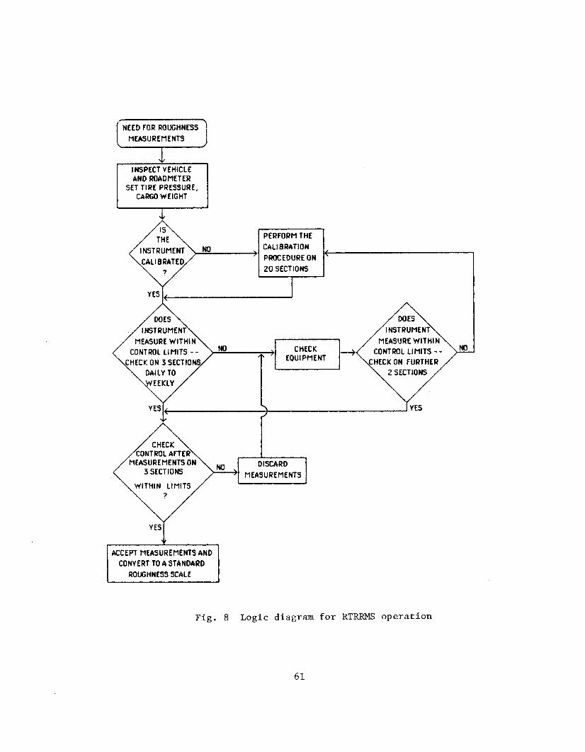
NEED FOR ROUGHNESS
AND ROADMETER SET TIRE PRESSURE,
CARGO WEIGH1
PERFORM THE CALIBRATION
7 ' PROCEDURE ON ' 20 SECTIONS
MEASURE WITHIN CONTROL LIMITS - - CONTROL LIMITS - -
MEASUREMENTS WITHIN LIMITS
ACCEPT MEASUREMENTS AND CONVERT TO A STANDARD
ROUGHNESS SCALE
Fig. 8 Logic diagram for RTRRMS operation
A one-person opera t ion i s probably bes t only f o r p r o j e c t s involving few measurements, where the time l o s t i n s topping the veh ic l e t o record and organize f i e l d notes i s not a problem.
b) Inspection. Before measurement, the equipment should be v i s u a l l y inspected t o ensure t h a t i t i s func t ioning co r rec t ly . The roadmeter l i nkages , t i r e p re s su re s , and c l e a n l i n e s s of the wheels need checking a t r e s t s tops o r a t l e a s t da i ly . During win ter , accumulation of i c e and snow on the veh ic l e should be kept i n check. When opera t ing i n muddy cond i t i ons , the accumulation of mud i n the wheels can be a problem.
c) Weather. Measurements should not be made during heavy r a i n o r s t rong o r gusty winds. On unpaved roads, measurements should not be made i f the sur face i s very wet o r s l i p p e r y , due t o the e f f e c t of mud on the wheels and the cool ing e f f e c t of water on the shock absorbers .
d) Speed control. It i s important t h a t the t e s t be run wi th in 5% of a cons tan t speed, s ince roughness r e s u l t s a r e speed dependent. The veh ic l e should be brought t o speed a t l e a s t s eve ra l seconds (100 m) before the s t a r t of the t e s t sec t ion . Usual ly, t he s tandard speed of 80 km/h w i l l be adopted.
e ) Lateral positioning. The veh ic l e should t r a v e l c o n s i s t e n t l y i n the wheeltracks. A s f a r a s p r a c t i c a b l e , potholes should be avoided s ince these can damage the roadmeter and i n v a l i d a t e the c a l i b r a t i o n . When potholes a r e included i n the measurement pa th , t h e i r presence and a b r i e f d e s c r i p t i o n should be noted.
f ) Warm-up. Rest s tops between measurements should be kept t o a minimum, and adequate warm-up time of 5 t o 10 minutes of the vehic le running a t t e s t speed should be allowed p r i o r t o t e s t . Longer per iods of 15 t o 20 minutes a r e necessary on roughness exceeding 8 m/km o r during cold o r wet weather. ( s ee Sect ion 4.3.3 f o r more s p e c i f i c gu ide l ines on s e l e c t i n g an appropr ia te warm-up time.)
4.3.2 Data processing. The number from the roadmeter should be converted t o a form of ARS t h a t i s convenient f o r t h a t p a r t i c u l a r roadmeter, such a s "counts/km," "in/mi ," o r "mm/km." ARS i s computed by d iv id ing the counts accumulated by the roadmeter while on the t e s t s ec t ion by the length of the sec t ion . If t he t e s t speed d i f f e r s from the s tandard , then i t should be noted a l so . (When da t a a r e taken a t s e v e r a l speeds, a convenient convention f o r i nd ica t ing speed i s t o add a
subsc r ip t t o ARS, e.g., ARS80 3.2, ARS50 = 3.8, e t c . )
The c a l i b r a t e d r e s u l t i s obtained by applying ARS i n the c a l i b r a t i o n equat ion (from Figure 7 ) :
L E [IRI] = A + B * ARS + C * ARS (16)

The value of E [IRI] i s the RTXRMS es t imate of the I R I on the measured sec t ion .
When repea t measurements have been performed, simple averaging of the o r i g i n a l ARS measures i s recommended, p r i o r t o conversion t o I R I .
Figure 9 shows a combination f i e l d form and work sheet t h a t can be used t o he lp convert the readings from the roadmeter t o c a l i b r a t e d roughness measures. In t h i s example, t h e procedure r equ i r e s t h ree repea t measurements on each s i t e . The c a l i b r a t i o n equat ion , shown a t the top of the f i g u r e , i s a l s o p lo t t ed f o r g raph ica l conversion t o I R I .
4.3.3 Temperature sensitivity test. The responsiveness of a RTRRMS t o roughness changes a s vehic le components "warm up" when t r a v e r s i n g rough roads. This t e s t should be conducted f o r each RTRRMS when i t i s f i r s t used t o determine the amount of warm-up time t h a t should be allowed f o r d a i l y opera t ion , and a l s o t o quickly i d e n t i f y veh ic l e s t h a t a r e unduly s e n s i t i v e t o temperature and thus unsui tab le f o r RTRRMSs.
A s e c t i o n of road should be found t h a t i s a t the roughest l e v e l a n t i c i p a t e d i n the study. It should have the minimum leng th required f o r a c a l i b r a t i o n s i t e , a s def ined i n Table 4. (The roughest c a l i b r a t i o n s i t e i s , i n f a c t , a good choice of l o c a t i o n f o r t h i s t e s t . ) The veh ic l e should be instrumented with a roadmeter and taken t o the se l ec t ed s i t e , where i t i s allowed t o cool down f o r a period of one t o two hours. The vehic le can be considered "cool" 15 minutes a f t e r the shock absorbers and t i r e s no longer f e e l warm t o the touch.
When the veh ic l e has cooled, "measure" the roughness of the warm- up t e s t s i t e a t the cons tan t t e s t speed. Record the time and the roadmeter "measure." Conversion t o the I R I s c a l e i s not necessary, a s t he i n t e r e s t here i s i n the r e l a t i v e change obtained. Immediately repea t t he t e s t , aga in recording the roadmeter reading and the time. Continue u n t i l the roadmeter readings reach a cons tan t l e v e l f o r a t l e a s t f i v e consecut ive runs.
The amount of time needed t o reach the s teady readings should always be used a s a minimum warm-up time. I f t he d i f f e r ence between the i n i t i a l and f i n a l reading i s more than 30%, a l t e r n a t i v e shock absorbers should be considered f o r the vehicle .
4.3.4 Control tests for RTRRMS time stability. Control s i t e s a r e s ec t ions of road t h a t a r e measured on a d a i l y o r weekly b a s i s t o determine wherther t he RTRRMS has changed s i n c e the l a s t check. They can a l s o be used t o determine and/or monitor the r e p e a t a b i l i t y of t he RTRRMS, and i t s s e n s i t i v i t y t o environmental condi t ions. One example of how con t ro l t e s t i n g can be in t eg ra t ed i n t o the opera t ing procedure
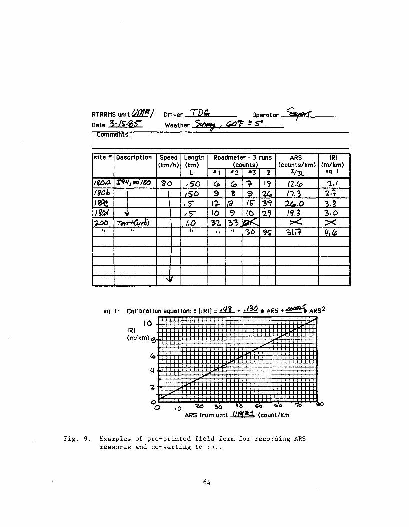
RTRRHS unit ah/ Driver TDG Opera tor % Date Weather h f m .I @f 5.
comments:
eq. I : C a l l b r a t t o n e q u s t t o n : E I I R l l = & + . I U ) m A R S + ~ ~ ~ ~ ~ ~
ARS from unt t
F i g . 9. Examples of p re -pr in ted f i e l d form f o r r e c o r d i n g ARS measures and c o n v e r t i n g t o I R I .

e s t a b l i s h e d f o r a p r o j e c t was shown i n Figure 8. I f measurements on the con t ro l s e c t i o n s do not f a l l wi th in l i m i t s e s t ab l i shed f o r the p r o j e c t , then the RTRRMS can be checked f o r d e f e c t s , and hopeful ly cor rec ted . A new c a l i b r a t i o n i s required unless a simpple reason f o r the change can be found and cor rec ted . I f i t i s determined t h a t t he veh ic l e ( o r roadmeter) has changed, then a l l d a t a gathered by t h a t RTRRMS s ince the l a s t con t ro l check should be discarded.
a) Objectives of control tests. Control t e s t s have been used mainly f o r t h ree purposes :
1) t o d e t e c t gradual changes i n the RTRRMS t h a t cause b i a s i n the data .
2 ) t o d e t e c t change i n the r e p e a t a b i l i t y of the RTRRMS, which r e s u l t s i n g r e a t e r e r r o r i n i nd iv idua l measurements.
3 ) t o determine whether environmental con td i t i ons ( r a i n , temperature, wind, e t c , ) have an impact on the measurements.
The con t ro l t e s t s a r e much more simple than the c a l i b r a t i o n t e s t i n g descr ibed i n Sect ion 4 .2 , i n o rde r t h a t they can be appl ied more f requent ly . They a r e used s o l e l y t o determine i f the RTRRMS has changed, and should not be used t o at tempt t o compensate o r c a l i b r a t e the RTRRMS. Thus, t he re ference I R I value f o r a con t ro l t e s t s i t e can be provided from the RTRRMS immediately a f t e r a c a l i b r a t i o n so t h a t p r o f i l e measurement i s not required.
b) Number of sites. A t l e a s t two c o n t r o l s i t e s should be used i n each check, covering a "smooth" s i t e and a "rough" s i t e . This i s because some e r r o r s a f f e c t only rough measurements and o the r s a f f e c t only smooth measurements. The RTRRMS can then be pe r iod ica l ly checked by comparing measurements t o the recorded re ference va lues , and comparison t o the v a r i a b i l i t y of measurements obtained i n previous checks.
c) Location of sites. By l o c a t i n g the s i t e s between the s torage loca t ion of othe RTRRMS and the roads being measured a s p a r t of the p r o j e c t , t he RTRRMS can be checked d a i l y with l i t t l e time o r e f f o r t . When a RTRRMS i s operated over a wide geographic a r e a , con t ro l s e c t i o n s convenient t o each a rea should be i d e n t i f i e d so t h a t s i t e s a r e a v a i l a b l e t o check the RTKRMS every day.
A s con t ro l s i t e s , t h e i r roughness i s assumed t o be cons tan t with t ime, and ca re should be taken t o ensure t h a t t h i s assumption i s reasonable. They should be por t ions of paved roads t h a t a r e l i g h t l y t rave led and a r e not scheduled f o r any maintenance over the course of t he pro jec t .

d) Site length. The length f o r a the con t ro l s i t e s should be cons i s t an t with the lengths of road s e c t i o n s normally measured i n the pro jec t . I f the main i n t e r e s t i s only the d e t e c t i o n of gradual changes i n RTRRMS s e n s i t i v i t y , then long con t ro l s i t e s a r e p re fe rab le , from 1.5 - 5 km. Shor te r s e c t i o n s can be used, but i t i s more d i f f i c u l t t o d i sce rn changes i n RTRRMS behavior because the RTRRMS r e p e a t a b i l i t y s u f f e r s on the s h o r t e r sec t ions . On s e c t i o n s 1.6 km long , normal v a r i a t i o n s should be wi th in +2%, al lowing de t ec t ion of smal le r changes on the order of +5% i n the RTRRMS. On con t ro l s ec t ions 320 m long , normal v a r i a t i o n s can be - +5%, with changes of - +lo% i n d i c a t i n g t h a t the RTRRMS has changed.
e) Repeat measures. Measurements can be repeated i n o rde r t o d i sce rn smal le r changes i n RTRRMS performance. This i s mainly use fu l when using s h o r t e r con t ro l s i t e s (1 km o r l e s s i n l eng th ) , and when the r e p e a t a b i l i t y of the RTRRMS is being checked.
f) Site identification. The beginning and end poin ts of each s i t e should be v i s i b l y i d e n t i f i a b l e from landmarks o r semi-permanent markings made f o r t h a t purpose. Immediately a f t e r c a l i b r a t i o n , a l l of the con t ro l s i t e s should be measured, j u s t a s any t e s t s e c t i o n s of road would be ( i . e . , cons tan t speed, RTRRMS "warmed up"). The measurements should be recorded f o r f u t u r e reference.
g) Acceptance levels. The con t ro l s i t e measures obtained with a RTRRMS should always f a l l wi th in an acceptab le range, where t h a t range i s determined by p r i o r experience with the u n i t and by the p ro j ec t ob jec t ives . It should be kept i n mind t h a t the con t ro l l i m i t s t o l e r a t e d on the con t ro l t e s t s ec t ions have an impact on the genera l l e v e l of accuracy t h a t can be assoc ia ted wi th the RTRRMS system. The acceptable range f o r a p a r t i c u l a r RTRRMS should be based on the i n i t i a l measurements of the con t ro l s i t e made wi th t h a t s p e c i f i c RTRRMS. A t l e a s t t h ree approaches can be taken f o r spec i f iy ing maximum and minimum l e v e l s of ARS t h a t a r e acceptable f o r a given RTRRMS. Using the no ta t ion t h a t ARS i s the cu r r en t va lue , and ARSinit i s the i n i t i a l value obtained when the con t ro l s i t e was f i r s t measured, these me:hods a re :
1 ) Percentage range, e.g., ARS = ARSinit - +5%
+1 dB, 2) dec ibe l range ( o r log increment) , e.g., ARS = ARSinifi, o r ~ O ~ ( A R S ) = ~ o ~ ( A R s ~ ~ ~ ~ ) t 0 . 0 5 log (AR~)
+5 "counts/km" 3) l i n e a r ARS range, e.g. ARS = ARSinit -
The f i r s t two a r e roughly equiva len t i n e f f e c t , and a r e appropr ia te when the measurement e r r o r i s roughly propor t iona l t o roughness. The t h i r d i s more appropr ia te when measurement e r r o r is f a i r l y cons tan t f o r the e n t i r e range of roughness covered i n the

p r o j e c t . When t h e range of i n t e r e s t covers mainly paved roads, and i n p a r t i c u l a r , smoother paved roads such a s major highways, then t h e t h i r d form i s recommended. When t h e range covers unpaved roads, o r extremely rough paved roads, then one of t he f i r s t two forms i s recommended.
The exac t th reshold s e l e c t e d must be determined from experience wi th t h e a c t u a l RTRRMS. h he 5% f i g u r e used i n t he above example may o r may not be appropr ia te . )
h) Data reporting, A s with o t h e r a r e a s of d a t a c o l l e c t i o n , pre- p r i n t e d f i e l d forms can he lp t o reduce human e r r o r and t o d e t e c t t r e n d s a s they s t a r t t o occur. Figures 10 and 11 show work s h e e t s t h a t have been used f o r t h i s purpose [9]. I n t h i s example, t h e c o n t r o l t e s t i n g covered both changes i n t he s e n s i t i v i t y of t h e RTRRMS and i n i t s r e p e a t a b i l i t y . Thus, repea t measures on t h e c o n t r o l s i t e s a r e required. Each week, s e v e r a l c o n t r o l s i t e s a r e measured f i v e times. From the work shee t (F igure l o ) , t he mean value f o r each s i t e i s computed, and t h e range of measures (an i n d i c a t i o n of r e p e a t a b i l t y ) i s noted. The log of t h e mean value i s compared t o t he l og of t h e o r i g i n a l measure, and t h e change i s p l o t t e d i n t h e top c h a r t i n Figure 11. This v i s u a l l y i n d i c a t e s any t r ends i n t he s e n s i t i v i t y of t he RTRRMS t o roughness. The range i s a l s o p l o t t e d , i n t he bottom c h a r t of Figure 11, s o t h a t i ncons t an t behavior i n d i c a t i v e of damaged components can be de t ec t ed ea r ly .
i) Frequency of testing, There is a trade-off involved i n e s t a b l i s h i n g the frequency with which c o n t r o l t e s t s a r e performed: f r r equen t c o n t r o l t e s t s t ake up time t h a t could i n s t ead be used ob ta in ing data . Yet , when problems a r e discovered from a c o n t r o l t e s t , l e s s d a t a is d iscarded i f t h e previous t e s t was performed recent ly . E s s e n t i a l l y , t h e c o n t r o l t e s t s should be repeated wi th s u f f i c i e n t frequency s o t h a t i f d a t a must be d i s ca rded , t h e l o s s i n time w i l l no t be too severe f o r t he p ro j ec t .

W O R K S H E E T F O R L D I C O N T R O L R U N S
R U N I LOGlO L D I V A L U E S ( m / k m ) I
- S U M L O G I O ( L D I ) X - -
c u r r e n t R A N G E = L D I
m a x - LDImin
5
S E C T I O N - ' i n i t i a l
- - D E V I A T I O N = Xinitial -
' c u r r e n t R A N G E = E N T E R O N R A N G E C O N T R O L C H A R T D E V I A T I O N = E N T E R O N M E A N C O N T R O L C H A R T
2 4
0 U
32
Fig. 10. Example of worksheet used for recording control test data (9)
68
26
d* '/3
3 2 - O*/S

L D I MEAN CONTROL CHART
I N I T I A L MEAN
TEST DATE
L D I RANGE CONTROL CHART
I I I I I I I I I I I I I I I I I
TEST DATE
Fig. 11. Example of worksheet f o r p l o t t i n g mean and range of RTRRMS c o n t r o l t e s t ( 9 ) .


CHAPTER 5
ESTIMATION OF IRI BY SUBJECTIVE EVALUATION (CLASS 4)
5.1 Descriptive Evaluation Method
When Class 1, 2, or 3 methods for measuring roughness are not feasible, estimations of the roughness on the IRI scale can be made subjectively. This approach may be used in the initial stages of a project to develop approximate assessments of the roughness, or in situations where an RTRRMS is not available. The descriptions used can also serve to acquaint the practitioner with the IRI scale, helping to visualize the meaning of the IRI values and the road conditions associated with them.
5.1.1 Method. The method provides adjective (and some quantitative) descriptions of the road surface conditions and ride sensations representative for several points on the IRI scale. These descriptions enable an observer traveling in a vehicle, and occasionally stopping to inspect the road, to recognize the conditions and to estimate the roughness. Photographs can be used effectively to support the method, but they can also be misleading because they tend to accentuate visual defects and minimize the shape or profile variations which relate most closely to roughness.
A method of this type has not been rigorously developed and proven, yet the success experienced with subjective ratings in the IRRE suggests that IRI values can be estimated with an accuracy that provides some indication of the road conditions at hand. Therefore, preliminary guidance is provided for this approach.
The accuracy of the method generally varies with the experience of the observer. Experienced observers will usually estimate roughness with an accuracy within 2 to 3 m/km, or about 30%, while new observers may have errors of 2 to 6 m/km, or about 40%. The estimates of IRI are therefore approximate and this method should not be used when mechanical means are available.
5.1.2 Description of the IRI scale. Figures 12 and 13 provide a series of descriptors for selected levels on the roughness scale. Figure 12 applies to surfaces of asphaltic concrete or surface treatment types, whereas Figure 13 applies to gravel and earth surfaces. These describe the typical categories of road, surface shape defects, ride sensation, and typical travelling speed associated with each given roughness level. The observer is expected to use all these to make an objective assessment of the roughness of a road while travelling along it. The most objective description relates to the surface shape defects

ROUGHNESS (m/km IRI)
0
2
4
6
8
10
12
14
16
18
20
22
24
Recently bladed surface of fine gravel, or soil surface with excel- lent longitudinal and transverse profile (usually found only in short lengths).
Ride comfortable up to 80-100 km/h. aware of gentle undulations or swaying. Negligible depressions (e.g. < 5mm/3m) and no potholes.
Ride comfortable up to 70-80 km/h but aware of sharp movements and some wheel bounce. Frequent shallow-moderate depressions or shal- low potholes(e.g. 6-30mm/3m with frequency 5-10 per 50m). Moderate corrugations (e.g. 6-20mm/0.7-1.5m).
Ride comfortable at 50km/h (or 40-70 km/h on specific sections). Frequent moderate transverse depressions (e.g. 20-40mm/3-5m at fre- quency 10-20 per 50m) or occasional deep depressions or potholes (e.g. 40-80mm/3m with frequency less than 5 per 50m). Strong corrugations (e.g. > 20mm/0.7-1 Sm).
Ride comfortable at 30-40 km/h. Frequent deep transverse depres- sions and/or potholes (e.g. 40-80mm/l-5m at freq. 5-10 per 50m); or occasional very deep depressions (e.g. 80mm/l-5m with frequency less than 5 per 50m) with other shallow depressions. Not possible to avoid all the depressions except the worst.
Ride comfortable at 20-30 km/h. Speeds higher than 40-50 km/h would cause exlreme discomfort, and possible damage to the car. On a good general profile: frequent deep depressions and/or potholes (e.g. 40-80mm/ I -5m at frequency 10-1 5 per 50m) and occasional very deep depressions (e.g. > 80mm/0.6-2m). On a poor general profile: frequent moderate defects and depressions (e.g, poor earth surface).
Fig. 12. Road roughness estimation scale for paved roads with asphaltic concrete or surface treatment (chipseal) surfacings.

ROUGHNESS (m/km IRI)
0
Ride comfortable over 120 km/h. Undulation barely perceptible at 80 km/h in range 1.3 to 1.8. No depress~ons, potholes or corrug- ations are noticeable; depressions < 2mm/3m. Typical high quali- ty asphalt 1.4 to 2.3, high quality surface treatment 2.0 to 3.0
4 Ride comfortable up to 100-120 km/h. At 80 km/h, moderately perceptible movements or large undulations may be felt. Defective surface: occasional depressions, patches or potholes (e.g. 5-15mm/3m or 10-20mm/5m with frequency 2-1 per 50m), or many shallow potholes (e.g. on surface treatment showing extensive ravelling). Surface without defects: moderate corrugations or large undulations.
Ride comfortable up to 70-90km/h, strongly perceptible movements and swaying. Usually associated with defects: frequent moderate and uneven depressions or patches (e.g. 15-20mml3m or 20-40mm/5m with frequency 5-3 per 50m), or occasional potholes (e.g. 3-1 per 50m). Surface without defects: strong undulat~ons or corrugations.
Ride comfortable up to 50-60 km/h, frequent sharp movements or swaying. Associated with severe defects: frequent deep and uneven depressions and patches (e.g. 20-40mm/3m or 40-80mm/5m with frequency 5-3 per 50m). or frequent potholes (e.g. 4-6 per 50m).
Necessary to reduce velocity below 50km/h. Many deep depres- sions, pothoies and severe disintegration (e.g. 40-80 mm deep with frequency 8-16 per 50m).
Fig . 13. Road roughness e s t i m a t i o n s c a l e f o r unpaved roads w i t h g r a v e l o r e a r t h s u r f a c e s .

which are expressed as a range of tolerances under a 3-m straight-edge; these can only be assessed by pedestrian inspection.
Note that both the descriptions and the associated IRI cover ranges of conditions at each level. This is necessary because the combinations of defects and severities vary widely, and because pavements at the same roughness level can have very different appearances.
The scale in the figures ranges from 0 to 24 mlkm IRI, as this is the range that has been covered in the IRRE and in other projects. The actual scale can continue to even higher levels, although roughness is so severe that travelling such roads is almost impossible. In describing benchmark levels of roughness, as done in the two figures, it is helpful to use the following descriptors:
a) Typical categories of road. The roads are first divided into the two categories of paved and unpaved because of characteristic differences between the roughness on these two types. The descriptions further refer to the quality of the shape (i.e., longitudinal profile) which can be expected for each type and quality of construction. They include the quality of shape after construction, and the extent and types of deterioration.
b) Surface shape defects. It is important to realize that roughness is related only to vertical changes in the level of the road in the wheelpaths of the vehicle, and that the superficial appearance of the surfacing can sometimes be misleading. Patches in the surfacing, or a coarse surface texture which results in loud tire noise may mislead the observer to overestimate roughness. Alternatively, a defect-free surface or a recent reseal may mislead the observer to underestimate the roughness if the road is very uneven. The observer must therefore become attuned to vertical surface irregularities. The characteristics used to describe surface shape are:
1) depressions: dish-shaped hollows in the wheelpaths with the surfacing in-place (by corollary, this includes humps of similar dimensions)
2) corrugations: regularly-spaced transverse depressions usually across the full lane width and with wavelengths in the range of 0.7 to 3.0 m (also termed washboarding)
3) potholes: holes in the surface caused by disintegration and loss of material, with dimensions of more than 250 mm diameter and 50 mm depth.

The size is indicated by the maximum deviation under a 3-m-long straight-edge, e.g., 6-20 mm/3 m, similar to a construction tolerance. The frequency is given by:
"occasional" = 1 to 3 per 50 m in either wheelpath
"moderate" = 3 to 5 per 50 m in either wheelpath
"frequent" = more than 5 per 50 m in either wheelpath
c) Ride sensation. In Figures 12 and 13, the "comfortable" ride is relative to a medium-size sedan car with regular independent shock- absorber suspension. Ride varies from car to car so more detailed descriptions are generally not transportable, but an observer can quickly become "calibrated" for a given vehicle. The ride sensation can be described in simple terms of the undulations and sharp movements experienced by the observer at a speed relevant to the level of roughness being defined. These descriptions can help considerably, but they must be developed for local conditions and vehicle types.
d) Travel speed. This indicates common travelling speeds on dry, straight roads without traffic congestion, with due consideration of care for the vehicle and the comfort of the occupants.
5.1.3 Personnel. The selection of observers should be made from those competent to make consistent, sound estimates of rating; typically, these will include professional engineers, technical personnel, etc. Usually, only one observer is used, but the accuracy of the result can be enhanced by the use of two or three persons.
5.1.4 Calibration. In order to calibrate to the scale, the observer should become thoroughly familiar with the salient features of each set of descriptions above. This could be called a "calibration by description." The final validity of such a calibration depends on how well the descriptions are tied to physical features of the road surface.
When possible, it is a valuable introduction for the observer to be driven over a few sections which cover a wide range of roughness and for which the IRI is known from physical measurements. If the vehicle to be used for the survey is very different in wheelbase or suspension characteristics from a mid-size passenger car sedan, special care should be taken to adjust: the ride descriptions used. Preferably, this should be done by "calibration" on a few physically measured sections. Alternatively, it can be done by pedestrian inspections and careful
. comparison of the shape measures with the descriptors.
5.1.5 Survey. On routes which are to be surveyed, the driver should be instructed to normally travel at 80 km/h on paved roads and 50 km/h on unpaved roads. At times, the observer may wish to vary the

speed t o t e s t the r i d e a b i l i t y aga ins t t he r i d e sensa t ion desc r ip t ions . An e s t ima te of average I R I should be made a t 1 km i n t e r v a l s (50 o r 70 seconds) , although on long, uniform rou te s , t h i s i n t e r v a l could be extended t o 2 km o r 5 km depending on the accuracy and d e t a i l required of t he survey. Occasional s tops f o r spot measurements a r e usefu l . The veh ic l e speed, su r f ace type, and weather condi t ions should be noted.
5.1.6 Data processing. The e s t ima te s f o r i nd iv idua l s e c t i o n s may be averaged t o determine the average roughness of the route. I f roughness l e v e l s range widely, by 100 percent f o r example, then the route should be subdivided i n t o nominally homogeneous segments f o r averaging.
5.2 Panel Rating of Riding Quality
Panel r a t i n g s of r i d i n g q u a l i t y have been implemented i n many p laces i n the past . Passenger observers r a t e the r i d i n g q u a l i t y of road sec t ions on an a r b i t r a r y s c a l e from e x c e l l e n t t o very poor ( impassable) , o f t e n quan t i f i ed on a s c a l e of 5 t o 0. Usually, t h i s i s l inked t o the S e r v i c e a b i l i t y Index (PSI) developed a t the AASHO Road Test o r a Ride Comfort Index. The PSI s c a l e i s l imi t ed i n t h a t i t was developed f o r roads of r e l a t i v e l y high q u a l i t y , i n comparison t o some of t he poorer roads covered i n t he I R R E and r ep resen ta t ive of condi t ions i n l e s s - developed count r ies . Thus the PSI s c a l e , a s c l a s s i c a l l y used i n t he United S t a t e s , only covers the low roughness end of the I R I scale.Data r e l a t i n g PSI t o I R I and o the r ob jec t ive roughness measures a r e scarce and i n c o n s i s t e n t , due i n p a r t t o the d i f f e r e n t methods t h a t a r e used by d i f f e r e n t agencies f o r est imatng PSI. Some of t he r e l a t i o n s h i p s a r e l i n e a r , while o t h e r s a r e not [ l o ] . A PSI value of 5 i s defined a s a pe r f ec t su r f ace , and i s thus equiva len t t o a 0 on the I R I s ca l e . A s roughness i nc reases , I R I i nc reases , and PSI decreases down t o 0 f o r a completely impassable surface.
Experience has shorn t h a t panel r a t e r s i n d i f f e r e n t coun t r i e s o r regions a t t r i b u t e widely d i f f e r e n t r a t i n g s t o a given roughness, commensurate with t h e i r expec ta t ions of r i d i n g qua l i t y . Thus panel r a t i n g s c a l e s a r e not comparable unless wel l anchored, and t h i s approach does not q u a l i f y a s a Class 4 method un le s s s p e c i f i c provis ions a r e made t o anchor the s c a l e through c a l i b r a t i o n aga ins t t he I R I .
The p o t e n t i a l advantage of t he panel r a t i n g s method i s t h a t the r a t i n g s assigned t o the road can be genuinely r ep re sen ta t ive of sub jec t ive opinion. For most a p p l i c a t i o n s of roughness d a t a , however, t h i s i s not the main p r i o r i t y . It i s u sua l ly more d e s i r a b l e t o use a roughness s c a l e t h a t has the same meaning from year t o year and from region t o region. Although sub jec t ive panel r a t i n g s can be "anchored" t o a t ime-stable s ca l e such a s I R I , t he method i s expensive and

inaccurate in comparison to the other methods available. Thus, panel ratings are not recommended for obtaining IRI measures, nor for any applications other than research projects where local public and/or profesisonal opinion is a variable of interest.


GLOSSARY
Accuracy - The root-mean-square value of the e r r o r when comparing measurements from a p a r t i c u l a r method t o those of a re ference method .
APL Trailer - A high-speed prof i lometer developed and operated by t h e French Labora to i re Cent ra l des Ponts e t Chaussees. The t r a i l e r uses a tuned mechanical system t o measure t h e su r f ace p r o f i l e of a s i n g l e wheel t rack over the frequency range of 0.5 t o 20 Hz.
APL 72 Waveband Analysis - An a n a l y s i s appl ied t o t h e p r o f i l e s i g n a l obtained from the APL T r a i l e r operated a t 72 km/h. The p r o f i l e i s f i l t e r e d i n t o shor t - , medium-, and long-wave bands. The content may be expressed a s :
a ) t he APL 72 "Energy" ( W ) , which i s t h e mean-square value of the f i l t e r e d p r o f i l e i n each waveband,
b) t he APL 7 2 "Equivalent Amplitude", which i s the amplitude of a s i n e wave having the same energy (E) ,
c ) t he APL 7 2 Index, which i s a va lue between 1 (worst) and 10 ( b e s t ) i n d i c a t i n g the r e l a t i v e q u a l i t y of the road.
The short-wave numeric i s most c l o s e l y c o r r e l a t e d t o the I R I and t o RTRRMS measures. A s i m i l a r s e t of t h r e e waveband numerics (CP) i s used by the Centre de Recherches Rout ie res i n Belgium.
APL 25 - See CAPL 25
ARSV - Average r e c t i f i e d s lope measured by a RTRRMS a t speed V. The recommended u n i t s a r e m/km, al though the u n i t s "inches/mile" and "mm/km" a r e a l s o popular. It i s the t o t a l RTRRMS suspension displacement ( i n both d i r e c t i o n s ) d iv ided by the d i s t a n c e t r a v e l l e d during t h e roughness measurement. Roadmeters based on the BPR Roughometer des ign produce measures of ARS/2, a s they accumulate displacement i n only one d i r ec t ion .
- Average r e c t i f i e d v e l o c i t y measured by a RTRRMS. It i s the average s t rok ing speed of the veh ic l e suspension during a roughness measurement. The ARV i s a d i r e c t measure of veh ic l e response t o roughness, such t h a t increased ARV always i n d i c a t e s increased veh ic l e v i b r a t i o n s , r ega rd l e s s of the measurement speed o r source of v ib ra t ions . ARV = ARS x speed, with the speed expressed i n app ropr i a t e un i t s .

BI - Abbrev ia t ion f o r Bump I n t e g r a t o r , t h e roadmeter used by t h e B r i t i s h TRRL, which i s a d e r i v a t i v e of t h e r o t a t i o n a l c l u t c h sys tem used w i t h t h e e a r l y BPR Roughometer. Measurements a r e u s u a l l y expressed i n "mm/km". The raw measure cor responds t o one-half t h e t o t a l accumulated suspens ion d e f l e c t i o n : t h u s B I r e s u l t s must be doubled t o o b t a i n ARS.
BI Trailer - A RTRRMS c o n s i s t i n g of a s p e c i a l single-wheeled t r a i l e r ins t rumented w i t h a B I roadmeter. The t r a i l e r h a s been developed by t h e TRRL, based on t h e d e s i g n of t h e e a r l i e r BPR Roughometer. I n t h e p a s t t h e B I T r a i l e r has been used on ly a t t h e speed of 32 kmlh; however, r e s u l t s from t h e IRRE demons t ra te t h a t i t can be used s u c c e s s f u l l y a t h i g h e r speeds .
BPR Roughometer - An e a r l y RTRRMS developed by t h e Bureau of P u b l i c Roads. It i s a single-wheeled t r a i l e r equipped w i t h a mechanical roadmeter employing a one-way c l u t c h , and h i s t o r i c a l l y h a s been opera ted a t 32 kmlh. The BPR Roughometer i s c o n c e p t u a l l y s i m i l a r t o t h e B I T r a i l e r , bu t i s t y p i c a l l y n o t a s rugged o r a s s t a n d a r d i z e d .
CAPL 25 - A numeric o b t a i n e d w i t h an APL T r a i l e r when o p e r a t e d a t 21.6 km/h. It i n c l u d e s an a n a l y s i s l t e s t procedure used widely i n France f o r e v a l u a t i o n of newly c o n s t r u c t e d roads. The CAPL 25 numeric i s computed f o r each 25 meter l e n g t h of roadway.
Counts/km, Counts/mile - Names used t o r e f e r t o t h e ARS s t a t i s t i c . The 1 I count" normal ly has a s s o c i a t e d w i t h i t a c e r t a i n increment of suspens ion d e f l e c t i o n measured by t h e roadmeter. These names have a l s o been used t o r e f e r t o t h e PCA sum-of-squares s t a t i s t i c , which i s q u i t e d i f f e r e n t from t h e ARS.
CP - C o e f f i c i e n t of Evenness, used by t h e Cen t re de Recherches R o u t i e r e s i n Belgium (CRR) a s a roughness measure. CP i s t h e average r e c t i f i e d v a l u e of a p r o f i l e t h a t h a s been f i l t e r e d w i t h a moving average. It h a s u n i t s of 50 CP = 1 mm. The CP numerics use b a s e l e n g t h s of approximately 2.5, 10, and 40 m when c a l c u l a t e d from APL 72 p r o f i l e s , and b a s e l e n g t h s of 2.5 and 15 m when c a l c u l a t e d from t h e APL 25 p r o f i l e . The CP(2.5) and CP(10) numerics can be o b t a i n e d u s i n g o t h e r p r o f i l e measurement methods, provided t h a t a s m a l l sample i n t e r v a l i s used. The CP(2.5) i s h i g h l y c o r r e l a t e d w i t h t h e I R I and RTRRMS measures.
GMR-Type Inertial Profilometer - An ins t rumented van developed by General Motors Research, and s o l d commercially by K. J. Law Engineers , Inc . , f o r measuring road p r o f i l e s a t highway speeds. The f i r s t p r o f i l o m e t e r s used an a c c e l e r o m e t e r , ins t rumented road- f o l l o w e r wheel , and ana log e l e c t r o n i c s t o measure p r o f i l e . More

recent models use noncontacting road-follower systems and digital signal processing methods. Since 1979, they have been equipped with software to compute IRI at the time of measurement. The computation program is called the Mays Meter Simulation.
Inches/mile - Name used to refer to an ARS measure of roughness. It denotes inches of suspension deflection per mile of distance travelled. 1 m/km = 63.36 inlmi.
IRI - International Roughness Index, equivalent to the ARS computed using a reference mathematical RTRRMS for a standard speed of 80 km/h. It is a mathematical property of the profile of a single wheeltrack. It is based on a calibration reference developed in an NCHRP program 121, which was later found to be the most suitable roughness index for international use in the IRRE.
IRBE - International Road Roughness Experiment held in Brasilia in 1982. The IRRE was conducted by research teams from Brazil, England, France, Belgium, and the United States.
K.J.Law Profilometers - see GMR-type inertial profilometer.
Mays Meter - A commercial roadmeter made by Rainhart Company. The transducer employs an optical encoder to produce electrical pulses that are mechanically accumulated by a one-way stepper motor connected to a strip-chart recorder. The meter measures the accumulation of suspension travel with units of Inchesl6.4, indicated by the advancement of paper in the strip-chart recorder. This measure is then converted to incheslmile by most practitioners. Although the transducer works properly on roads of all roughness levels, the stepper motor has response limits that cause it to count improperly at high roughness levels.
Mays Meter Simulation - A commercial computer program offered by K. J. Law Engineers, Inc. with the GMR-type profilometer. In some versions, the program exactly matches the IRI (using units of incheslmile rather than mlkm); in others, the program uses the IRI car parameters with a half-car simulation, rather than the quarter-car specified for the IRI.
-/lam - A name used to describe the ARS measure. It is commonly used with the BI Trailer. Measures from the BI roadmeter are generally reported with half the value that would be used for ARS. Thus, 1 m/km ARS = 500 mmlkm BI.
Moving Average - A method of analysis used to compute a roughness index from a measured profile. The analysis smooths the profile by replacing each point with the average of adjacent points over a
8 1

1 i n 1975 . I n concept , QI i s i d e n t i c a l t o I R I , and i n p r a c t i c e , the two i n d i c e s a r e very h ighly co r r e l a t ed . It i s an ARS measure wi th a r b i t r a r y u n i t s of "counts"/km, and i s based on an e a r l y re ference s imula t ion of a RTRRMS. The o r i g i n a l QI was an abbrevia t ion f o r Quarter-car Index, and was based on the readings taken from a p a r t i c u l a r p iece of hardware a s operated on paved roads i n Braz i l . Due t o a number of equipment d e f e c t s and e r r o r s i n c a l i b r a t i o n methodology, the o r i g i n a l QI measure cannot be r e p l i c a t e d today using the same method. Since the beginning of the
1 >
2 )
3 )
PICR p r o j e c t , t h e r e have been th ree types of QI da ta :
QIr - A profi le-based roughness s t a t i s t i c developed by Queiroz and o t h e r Braz i l i an r e sea rche r s t o rep lace the QI c a l i b r a t i o n sca le . QIr i s computed from a s i n g l e s t a t i c a l l y measured p r o f i l e , t y p i c a l l y obtained with the rod and l e v e l method, us ing a weighted sum of two RMSVA s t a t i s t i c s ca l cu la t ed from baselengths of 1.0 and 2.5 m:
The above equat ion r equ i r e s the RMSVA measures t o have the u n i t s of l/km (.001/m), a s obtained when p r o f i l e e l e v a t i o n i s measured i n mm. Designed with rod and l e v e l prof i lomet ry i n mind, QIr cannot be measured wi th a s many methods a s I R I . Also, the c o r r e l a t i o n s with RTRRMSs a r e not q u i t e a s good f o r some condit ions.
QI* - The "ca l ib ra t ed" measures from RTRRMSs, used f o r a l l of t h e d a t a measured i n t he PICR P r o j e c t , a s reported and s to red i n t he Braz i l i an computer d a t a f i l e s . The c a l i b r a t i o n used was not complete and d i d not c o r r e c t the measures t o the QI sca lg f o r a l l su r f ace types. On a s p h a l t i s concre te roads, QI i s equiva len t t o QI , ; however, QI numerics a r e l a r g e r than corresponding QIr measures on unpaved roads, and s u b s t a n t i a l l y h igher (sometimes by 100%) on su r f ace t reatment roads.
* Q1w - Engineering consu l t an t s t o the World Bank have been reprocessing roughness d a t a obtained during the I C R Pro jec t . The r e s u l t i n g cos t equat ions , when publ ished, w i l l d i f f e r from the o r i g i n a l ones, a s they have been resca led t o br ing the QIw s t a t i s t i c c l o s e r t o the QI r s t a t i s t i c on a l l types of roads.
' ~ e s e a r c h on t h e I n t e r r e l a t i o n s h i p s between Costs of Highway Construct ion, Maintenance, and U t i l i z a t i o n . (The Braz i l i an Transpor ta t ion Planning Agency - GEIPOT)

s p e c i f i e d base length. The smoothed p r o f i l e i s sub t r ac t ed from t h e o r i g i n a l t o cance l t he long wavelength geometry. The r e s u l t i n g f i l t e r e d p r o f i l e i s summmarized by an average r e c t i f i e d va lue , o r by an RMS value. With a proper choice of baselength (1.5 - 3 m), high c o r r e l a t i o n s e x i s t with RTRRMSs. The a n a l y s i s i s mainly used t o i s o l a t e roughness p r o p e r t i e s of i n t e r e s t t h a t o f t e n cannot be de tec ted wi th RTRRMSs.
=RA Meter - A roadmeter developed and used by the Aus t r a l i an Road Research Board (ARRB), toge ther wi th a re ference veh ic l e t o de f ine a NAASRA RTRRMS. The NAASRA roadmeter was found capable of measuring ARS and ARV s t a t i s t i c s over the f u l l roughness range. The NAASRA RTRRMS used i n A u s t r a l i a has been "ca l ib ra t ed" by holding one RTRRMS i n s to rage a s a r e f e rence , and c o r r e l a t i n g the o t h e r RTRRMSs wi th it.
PCA Meter - An instrument s i m i l a r t o a roadmeter i n which d i s c r e t e l e v e l s of suspension displacement a r e summed independently. Most PCA meters can a l s o be used a s simple roadmeters simply by adding the readings from a l l of the counters toge ther .
PC& sum-of-squares - a measure obtained from a PCA meter , where the readings from the d i f f e r e n t counters a r e each weighted before they a r e added. The r e s u l t i n g measure was intended t o be i n d i c a t i v e of a mean-square response, but i t has been shown the the weighted sum has no r e l a t i o n t o any phys ica l v a r i a b l e s [ 2 ] . The use of t h i s measure i s not recommended.
Profilometer - A. mobile instrument used f o r measuring t h e long i tud ina l p r o f i l e of roads. A prof i lometer has i t s own means f o r c a l i b r a t i o n , o t h e r than the empir ica l regress ion methods needed f o r RTRRMS. The p r o f i l e measured may not be t r u e i n the sense t h a t i t may not inc lude a l l wavelengths, y e t can be v a l i d f o r a p p l i c a t i o n s i n road roughness measurement and c a l i b r a t i o n . Depending on the ins t rument , t he p r o f i l e may be s to red and/or processed on board the prof i lometer t o y i e l d summary numerics dur ing measurement. high-speed prof i lometers a r e instruments t h a t can be used a t normal road speeds, whereas static prof i lometers a r e used a t walking speeds ( o r slower).
QCS - Q u a r t e r c a r s imulat ion. A mathematical model of a veh ic l e t h a t has a body and s i n g l e t i r e . It computes t he response of a re ference veh ic l e from measured p r o f i l e input .
QI - The o r i g i n a l road roughness s t a t i s t i c adopted f o r use a s a c a l i b r a t i o n s tandard i n the Braz i l i an PICR user-cost p r o j e c t begun

QI can be considered a s an e a r l i e r vers ion of I R I . Although the o r i g i n a l d e f i n i t i o n s of QI a r e d i f f i c u l t t o apply with confidence i n many cases , t h e d a t a from the IRRE i n d i c a t e t h a t f o r a l l p r a c t i c a l purposes, QI can be considered t o be I R I wi th d i f f e r e n t u n i t s and an o f f s e t . The conversion equat ion recommended i s :
E [ Q I ] "counts/km" = 14 I R I (m/km) - 10
RARSsO - Reference average r e c t i f i e d s lope a t 80 km/h. This i s t he more t echn ica l name f o r I R I .
RABV - An abbrevia t ion f o r re ference ARV. RARV = ARS x speed, where the ARS i s obtained from the QCS of the re ference vehic le .
Repeatability - The expected s tandard dev ia t ion of measures obtained i n repea t t e s t s , using the same instrument on a s i n g l e , randomly- s e l e c t e d road.
Reproducibility - The standard dev ia t ion of t he e r r o r included i n s i n g l e measurement, r e l a t i v e t o a re ference measure. The r e p r o d u c i b i l i t y of an instrument inc ludes e r r o r s t h a t a r e sys temat ic wi th respec t t o t h a t ins t rument , but random with respec t t o a p a r t i c u l a r t e s t .
Resolution - The sma l l e s t increment t h a t can be measured with a p a r t i c u l a r ins t rument , due t o i t s design.
Ridemeter - An ins t rumenta t ion package t h a t i s i n s t a l l e d i n a veh ic l e t o measure v ib ra t ions . Sometimes, t he word Ridemeter i s used i n o t h e r documents a s a s u b s t i t u t e f o r the word Roadmeter; o the r times the word Ridemeter i s appl ied t o instruments t h a t measure veh ic l e response t o determine r i d e q u a l i t y , r a t h e r than the roughness of the road.
RMSVA - Abbreviation f o r the words "Root Mean Square V e r t i c a l Acceleration." This measure was proposed by McKenzie and s r inarawat2 a s a profi le-based c a l i b r a t i o n reference. The s t a t i s t i c i s a func t ion of a measured p r o f i l e s i g n a l , toge ther with a s i n g l e baselength parameter. The VA ( v e r t i c a l a c c e l e r a t i o n ) i s def ined a t l ong i tud ina l pos i t i on x a s :
2 " ~ ~ o t Mean Square V e r t i c a l Acce lera t ion (RMSVA) a s a Basis f o r Mays Meter Ca l ib ra t ion , " Braz i l P ro j ec t Memo BR-23, Center f o r Transpor ta t ion Research, The Univers i ty of Texas a t Aust in, February 1978

where Y(x) i s the s i g n a l amplitude ( p r o f i l e e l e v a t i o n ) a t pos i ton x , and b i s the baselength parameter. A s def ined by the above equat ion , RMSVA has u n i t s of v e r t i c a l a c c e l e r a t i o n , but has no r e 1 a t i o n s h . i ~ wi th the a c t u a l s p a t i a l a c c e l e r a t i o n of the p r o f i l e . In s t ead , i t i s simply a measure of mid-chord dev ia t ion with a
2 s c a l e f a c t o r of 2 /b . The RMSVA s t a t i s t i c was used t o de f ine the QIr c a l i b r a t i o n s tandard i n t he PICR P r o j e c t , and has a l s o been used t o de f ine a RTRRMS c a l i b r a t i o n s tandard f o r use i n Texas.
Roadmeter - An instrument t h a t i s i n s t a l l e d i n a veh ic l e t o t ransduce and accumulate the suspension d e f l e c t i o n s t h a t occur when the veh ic l e t r a v e r s e s a road. The r e s u l t a n t measure i s p ropor t iona l t o the t o t a l accmulated suspension d e f l e c t i o n t h a t occurred during the t e s t .
Roughness of a road - The v a r i a t i o n i n su r f ace e l e v a t i o n along a road t h a t causes v i b r a t i o n s i n t r a v e r s i n g vehic les . The s tandard summary s t a t i s t i c t h a t q u a n t i f i e s t h i s v a r i a t i o n i s the I R I .
RTRRMS - Response-type road roughness measuring system. These systems c o n s i s t of a passenger c a r or a towed t r a i l e r having e i t h e r one o r two wheels, p lus a roadmeter i n s t a l l e d t o measure suspension de f l ec t ions .
Single-track RTRRMS - A towed t r a i l e r supported by a s i n g l e wheel, instrumented wi th a roadmeter. The roughness measure obtained a p p l i e s only f o r a s i n g l e wheeltrack.
Slope Variance (SV) - A measure of road roughness t h a t i s the var iance of a s i g n a l produced by the e a r l y AASHTO Prof i lometer and CHLOE Profi lometer . As used t o desc r ibe roughness, Slope Variance r e f e r s t o the var iance of a s i g n a l o r "p ro f i l e " obtained by a s p e c i f i c method. The Slope Variance i s more s e n s i t i v e t o the choice of p r o f i l e measurement method than t o roughness, and does not desc r ibe a s tandard roughness measure. (The "true" var iance of t he s lope of a road p r o f i l e i s i n f i n i t e , s i n c e the t r u e p r o f i l e i nc ludes t e x t u r e e f f e c t s . ) Although the simple geometry of the e a r l y "profi lometers" impl ies t h a t Slope Variance can r e a d i l y be computed mathematically from more accura te p r o f i l e measures, the e a r l i e r ins t rumenta t ion systems had qu i rks and complexi t ies t h a t have not been we l l documented, so t h a t e s t ima te s of Slope Variance made from imeasured p r o f i l e s a r e not equiva len t t o outputs of t he o ld instruments . Slope Variance measures have never been found t o be very compatible wi th the ARS and ARV measures obtained with RTRRMS s .
TRRL Beam - A q u a s i - s t a t i c prof i lometer developed by TRRL t h a t measures a p r o f i l e i n 3-m s e c t i o n s ( t h e l eng th of the instrument) . The
Beam is designed with developing country environments in mind, and is lightweight, portable, and self-contained. It includes a battery-powered microcomputer that controls the measurement process and can automatically calculate roughness statistics.
TBBL Laser Profilometer - A high-speed profilometer developed and operated by TRRL. The profilometer uses several noncontacting laser height sensors, spaced over the length of a trailer, to compute surface profile as the trailer is towed at highway speeds.
Two-track RTRRl4!3 - A RTRRMS based on a passenger car, light truck, or a towed two-wheel trailer. The measure obtained is a function of the roughness in two wheeltracks.
VTI Laser Profilometer - Profilometer van developed and operated by the Swedish VTI. This profilometer operates at normal highway speeds and uses a combination of accelerometers, noncontacting height sensors, and digital computation to measure a number of parallel longitudinal profiles distributed across the 2.5 to 3.5 m width of the highway lane.
Waveband - A range of spatial frequencies (wavenumber = l/wavelength). The waveband includes only the wavenumbers that lie inside its range.
Wheeltrack - The path followed by the tire of a vehicle traversing a road. Each lane has two travelled wheeltracks. When measuring roughness, the wheeltrack should parallel the centerline insofar as possible.

REFERENCES
1. Sayers M. W., G i l l e s p i e , T. D., and Quei roz , C., The I n t e r n a t i o n a l Road Roughness Experiment: E s t a b l i s h i n g C o r r e l a t i o n and a C a l i b r a t i o n Stan- dard f o r Measurements, World Bank Technical Paper No. 45, Wash., D.C., 1986.
2. G i l l e s p i e , T. D., Sayers, M. W. and Segel , L., C a l i b r a t i o n of Response-Type Road Rougnness Measurement Systems, NCHRP Report 228, 1980.
3. Methodology f o r Road Roughness P r o f i l i n g and Rut Depth Measurement, Cont rac t No.DTFH61-83-C-00123, Federa l Highway Adminis t ra t ion, The Univers i ty of Micigan, J u l y 1983.
4. Analyseur de P r o f i l e en Long - APL 72. B u l l e t i n 1 B AC 76, Ma te r i e l s des Labora to i res des Ponts e t Chaussees, Par i s .
5. "Measurement of t h e Evenness of Pavement Courses Using t h e APL 25 Dynamic Logi tud ina l P r o f i l e Analyzer." Pre l iminary Draf t Procedure, Labora to i r e Cen t r a l des Ponts et Chaussees, Div is ion des S t r u c t u r e s et Cha rac t e r i s t i ques des Chaussees, Par i s .
6. Spangler , E. B. and Kel ly , W. J., "GMR Road Prof i lometer - A Method f o r Measuring Road P r o f i l e , " Highway Research Record 121, Wash., D.C., 1966.
7. S p e c i f i c a t i o n No. S8300m, Road Roughness Surveyor, K. J. Law Engineers , Inc., Farmington H i l l s , Michigan, Nov. 1983.
8. Pa te rson , W. D. O., "Accuracy of Cal ibra ted Roughness Surveys," Presen ted a t t he ASTM Symposium on Roughness Methodology, Bal Harbour, F lo r ida , December 1983.
9. Visser, A. T., and Curtayne, P. C., "The Routine Operat ion, C a l i b r a t i o n and Control of t h e Linear Displacement I n t e g r a t o r , " Report No. RC/7/82, Nat ional I n s t i t u t e f o r Transport and Road Research, P r e t o r i a , 1982.
10. Pa te rson , W. D. O., P r ed i c t i on of Road D e t e r i o r a t i o n and Maintenance E f f e c t s : Theory and Quant i f ica t ion . Highway Design and Maintenance Study, Vol. 3. World Bank, T ranspo r t a t i on Department, Washington, D.C. 1986.

C a d s Hirxh SRL Galeria G u m Florida 165 4rh F lmOfc 4531465 1333 Buenos Arcs Tel 30-7122 33-1787
AUSlMUClPIVUANew GUINEA, m, S a O m N IUANW, AW VANUAnJ
obCine Overseas Dotumenr D e l q Box 3% GPO Sydney NSW 2MI Australia Tel 1021 282-1614
AUSlllU Gerold and Co A 1011 Wlrn Crakn 31 Tel I02221 52 22 35
uu4RAw MEMRB PO Box 22103 Manama Town 3 1 7 Tel 232934
MNGWLSn Micro ndusnles DMlopmenr Assisrarre
Sotiefy IMlDhSI GPO Box800 Dhaka Tel 326427
mww Puol~cations C 6 Nar~ons UPIK Av du Roi 202 "&I Brussels Tel 021538 51 69
aRML Publicacces Tecnicas In[ernac~onas ~ tda Rua Peixoto Gomide. 209 01409 ho Paulo SP Te I01 1 1 257-1610. 258-8167 258-8442
CANADA Le D i h w r CP 85 1501 r u e h p t r e Bouchewille. O u e k Canada 148 5E6 Tel 15141 641-1334
cnlu Ed~rorial Renac~mmro Miraflores 354 iar r iqo Te 35244
COLOYUA En Im Ltdd 4oa!l640 Aero 34270 Bogora D E 'el 24542645
COSTA RKA LGfefid Trejos Calle 11-13 Av Fernandez Guell San Jose Tel 303-2858 5 4
mmus MEMRDB PO Box 2098 NlCOSid Tel 21 99133
D E W SdmfundsLneralur Roremrns Alle I1 DK- 1970 CopmMgen V Tel 01.35 1942
€ G w T , A I W ~ O C Al Ahram Galaa Sam Cairo Tel 758333
Akdleemnwr Kirjarauppa PO Box 128
FMlYQ World Bank Publicarms M Avewe dlena 75 1 I6 Paris Tel 723-54-2 1
UNO-Vemg D-53W Bonn I Simrotarrasse 23 Tel 102281 21 29 40
uma MEMRB 24 IoWdamou Streer Athens. I I635 Tel 7018082 7016W5
HONG K M . MALAU h a 2 m Lrd 6 Fl 4 6 Prince € h a r d Road W Kowlwn "ong Kong Tel 3-80529415
lllDU UBS Publisherr' D~rrributon Lrd Porr Box 7015 A n w Road N w Delhl 110002 Tel 17MOI -3
10 Firs! Main Road Gdndhl N a w Bangalae j6000P Tel 28094 29206
Acejay Chamten P 0 Box 7% 5 Wallace Streu Bombay 400001 Tel 2a0%2. 2 m 2 1 266971
l l . 8 C M i n ~ h e e idm Calcuna 7 ~ 1 i Tel 212451 249473
71 188 I (CAI Swamp Nagar Kdmpu 2OBOO2 Tel 81300
Sivagaqa Road Nungam@drkam Madras b00034 Tel 476355
INDou€nA R ndira bmired l Sam Rarulangi 37 Jakdild PUU~ PO Box 181 Tet @I418
ImANo TDC Publishen 12 Nm Frederick Srreet Dublin I Tei 744835
ITALY Cicora Comm~ss~onana h n m i SPA Via Lamarma 45 Casclla Posrale 552 MI21 Flotence Tel 579 7511213
4b1djan 04 Plateau Tel 22-20-55 and 32MM2
W A N Easrem W S e ~ c e lEBSl 37-3 Hongo 3 4 h m Bunkpku I1 3 rev Tel 1031 438-261 1 - MEMRB PO Box 3143 Jam1 Amman
W A Ahica W h c e IEA 1 Ltd P 0 Box 45245 Nd~robi Tel 2364 11330272
KORUACCVIUCOC Pdn Korea aOOk Corpdrim D O Box 101 KwarqMdmun Seoul 'el 723.1421
KUWAn MEMRB PO Box 546s K ~ w d ~ t r e 421843
MmcO INFOTEC Sdn Lwenzo 153-1 1 Cot del Valle Delea
Beniro Judlez 03 IW Mex~co Cify D F Tel 559-521 1
MOROCCO MEMRB 2 iue Moliere Raciw Cdiablanca Tel 259461
Tna NCrnaUllW Medical BooCs Europe W IMBEl Nwrdaval 38 724 1 BL Lothem Tel rK73M866
NEW 2- R Hill dnd Son L!d Prware Bag New MaRer Auckland Tel 5481 19
Nwmn Unlvefsify Rns bmlted Three C r ~ s Building Jericho Prrvare Mall Bag 5095 ICadan Te :-22 41 13%
NORWAY Tar,--KaO lohan AS PO sox Il77Senoum CSIC ' Te 621 90 12tU
PAKISTAN M 7 a 9001: Agency 65 Shanrah-e-Ouaid-e-&am P 0 @ox No 729 Lahore 3 Tel 65839
PANAMA E31cones L,brer!a Cuirural Paramena. SA Av 7 Ersana I6 Pardma Zone 1
Tc :!-5628
nmr Ediroria~ Derarrolo 24 Apanaao 3824 ICd 242 OE 1M Cima I Tel 28.53.80
Tn€ PHIUPPINES Mationdl Bwk Srwe PO Box 1934 Metro Uarila Tel 43-92-12
PomuGU Ciwafia Pon~gal Rua DO Carm 70-74 I2W LlStm Tel 32 82 20
Jar! Oak Store PO Box 3'96 Riyadh- I471 Saudi 4,aDla Tel 47731W
,r awre 1953 :e4!83.1?98
SPUN V.llr"a~ P e w LiDrOs SA Cdsrello 37 28W I Madrid Te 276-997
W U N W A N D M ~ Ldke House BCOkSkOp P 0 Box 244 IW. 511 Chinampaldm A Gardinec
Mawatha Colomtc 2 Tel 32104
SWEDEN Fm j q l e :1rIe5 ABCE Frluer Kungl Hovtokhandel Reger~mpyran 12 Box 163% 5-103 27 Srotkholm Tel 08 23 89 W
Fol SUDSCflpiiOn ordm Wennergren-Will~arm AB Box 30004 8-1 04 25 Srocknolm Tel 08-54 1200
wmmuND Librair~e Payor 6 rue G r e w Case wrrai 381 CH I21 1 G e r m I I Tel 31-89-9
TANZANLA Oxford Ur~wvrry Press P 0 Box 5299 Ddr er Salaam
29209
WUND Cenrrai Decanvem Srore 3M S om Road Bdngrok Tel 2336930-9
Trntdad West lndics Tel i-18091 62.5654
TUNIS4 Scc ere Tun~sienne de Diffusion 5 Averwe de Canhdge Tmr :el 255.1103
lum Haret Kirdoevi A S 4h9 lr!lkla~ Caaaeri 3evog~-lr;an~ul Te ' 4 4 94 :Dl?!
Lgarda Bookmop P O Boa 7'45 Kampala Tel 437%
U r n 0 MM LMlRAIEI MEMRB
PO Box 3 Alror Harnoshlre GU 34 2f f i ~ r l r e d Kinadom Tel Allon iW8
V I N U U M mend del Este Aprdo M 337 Caracas IWO-A Tel 32 23 01133 26 04
WEmnNUYOA Wesley 80ol;sm PO Bbx 207 m a Tel 22 822