Embed Size (px)
Citation preview

Guide for Gamelin’s Complex Analysis
James S. CookLiberty University
Department of Mathematics
Fall 2014

i
purpose and origins
This is to be read in parallel with Gamelin’s Complex Analysis. On occasion, a section in this guidemay have the complete thought on a given topic, but, usually it is merely a summary or commenton what is in Gamelin. It follows that you probably should read Gamelin to begin then read this.I’ll let you find the right balance, but, I thought I should clarify the distinction between these notesand other Lecture Notes which I’ve written which intend more self-sufficiency.
There are two primary audiences for which these notes are intended:
1. students enrolled in my Math 331 course at Liberty University,
2. students interested in self-study of Gamelin who wish further guidance.
Most of the course-specific comments in these notes are clearly intended for (1.). Furthermore,these notes will not cover the whole of Gamelin. What we do cover is the basic core of undergrad-uate complex analysis. My understanding of these topics began with a study of the classic textof Churchill as I took Math 513 at NCSU a few years ago. My advisor Dr. R.O. Fulp taught thecourse and added much analysis which was not contained in Churchill. The last time I taught thiscourse, Spring 2013, I originally intended to use Freitag and Busam’s text. However, that textproved a bit too difficult for the level I intended. I found myself lecturing from Gamelin more andmore as the semester continued. Therefore, I have changed the text to Gamelin. Churchill is a goodbook, but, the presentation of analysis and computations is more clear in Gamelin. I also havelearned a great amount from Reinhold Remmert’s Complex Function Theory [R91]. The historyand insight of that book will bring me to say a few dozen things this semester, it’s a joy to read,but, it’s not a first text in complex analysis so I have not required you obtain a copy. There areabout a half-dozen other books I consult for various issues and I will comment on those as we usethem.
Remark: many of the quotes given in this text are from [R91] or [N91] where the original source iscited. I decided to simply cite those volumes rather than add the original literature to the bibliog-raphy for several reasons. First, I hope it prompts some of you to read the literature of Remmert.Second, the original documents are hard to find in most libraries.
For your second read through complex analysis I recommend [R91] and [RR91] or [F09] for thestudent of pure mathematics. For those with an applied bent, I reccommend [A03].
format of this guide
These notes were prepared with LATEX. Many of the definitions are not numbered in Gamelin andI think it may be useful to set these apart in this guide. I try to follow the chapter and sectionclassification of Gamelin in these notes word for word, however, I only include the sections I intendto cover. The wording of some definitions, theorems, propositions etc. are not necessarily as theywere given in Gamelin.
James Cook, November 11, 2014 version 1.11

ii
Notations:
Some of the notations below are from Gamelin, however, others are from [R91] and elsewhere.
Symbol terminology Definition in Guide
C complex numbers [1.1.1]Re(z) real part of z [1.1.1]Im(z) imaginary part of z [1.1.1]z complex conjugate of z [1.1.3]|z| modulus of z [1.1.3]C× nonzero complex numbers [1.1.6]C[z] polynomials in z with coefficients in C [1.1.8]R[z] polynomials in z with coefficients in RArg(z) principle argument of z [1.2.1]arg(z) set of arguments of z [1.2.1]eiθ imaginary exponential [1.2.4]|z|eiθ polar form of z [1.2.4]ω primitive root of unity [1.2.12]C∗ extended complex plane [1.3.1]C− slit plane C− (−∞, 0] [1.4.1]C+ slit plane C− [0,∞) [1.4.1]f |U restriction of f to U [1.4.2]n√z n-th principal root [1.4.4]
Argα α-argument of [1.4.5]ez complex exponential [1.5.1]Log(z) principal logarithm [1.6.1]log(z) set of logarithms [1.6.2]zα set of complex powers [1.7.1]sin(z), cos(z) complex sine and cosine [1.8.1]sinh(z), cosh(z) complex hyperbolic functions [1.8.2]tan(z) complex tangent [1.8.3]tanh(z) complex hyperbolic tangent [1.8.3]limn→∞
an limit as n→∞ [2.1.1]
limz→zo
f(z) limit as z → zo [2.1.14]
C0(U) continuous functions on U [2.1.16]Dε(zo) open disk radius ε centered at zo [2.1.19]∂S boundary of S [2.1.21][p, q] line segment from p to q [2.1.22]f ′(z) complex derivative [2.2.1]JF Jacobian matrix of F [2.3.1]ux = vyuy = −vx
CR-equations of f = u+ iv [2.3.4]
O(C) entire functions on C [2.3.8]O(D) holomorphic functions on D [2.3.12]
You can also use the search function within the pdf-reader.

Contents
I The Complex Plane and Elementary Functions 1
1.1 Complex Numbers . . . . . . . . . . . . . . . . . . . . . . . . . . . . . . . . . . . . . 1
1.1.1 on the existence of complex numbers . . . . . . . . . . . . . . . . . . . . . . . 5
1.2 Polar Representations . . . . . . . . . . . . . . . . . . . . . . . . . . . . . . . . . . . 7
1.3 Stereographic Projection . . . . . . . . . . . . . . . . . . . . . . . . . . . . . . . . . . 12
1.4 The Square and Square Root Functions . . . . . . . . . . . . . . . . . . . . . . . . . 12
1.5 The Exponential Function . . . . . . . . . . . . . . . . . . . . . . . . . . . . . . . . . 14
1.6 The Logarithm Function . . . . . . . . . . . . . . . . . . . . . . . . . . . . . . . . . . 16
1.7 Power Functions and Phase Factors . . . . . . . . . . . . . . . . . . . . . . . . . . . . 17
1.8 Trigonometric and Hyperbolic Functions . . . . . . . . . . . . . . . . . . . . . . . . . 19
II Analytic Functions 23
2.1 Review of Basic Analysis . . . . . . . . . . . . . . . . . . . . . . . . . . . . . . . . . . 23
2.2 Analytic Functions . . . . . . . . . . . . . . . . . . . . . . . . . . . . . . . . . . . . . 29
2.3 The Cauchy-Riemann Equations . . . . . . . . . . . . . . . . . . . . . . . . . . . . . 33
2.3.1 CR equations in polar coordinates . . . . . . . . . . . . . . . . . . . . . . . . 38
2.4 Inverse Mappings and the Jacobian . . . . . . . . . . . . . . . . . . . . . . . . . . . . 40
2.5 Harmonic Functions . . . . . . . . . . . . . . . . . . . . . . . . . . . . . . . . . . . . 42
2.6 Conformal Mappings . . . . . . . . . . . . . . . . . . . . . . . . . . . . . . . . . . . . 44
2.7 Fractional Linear Transformations . . . . . . . . . . . . . . . . . . . . . . . . . . . . 48
III Line Integrals and Harmonic Functions 53
3.1 Line Integrals and Green’s Theorem . . . . . . . . . . . . . . . . . . . . . . . . . . . 53
3.2 Independence of Path . . . . . . . . . . . . . . . . . . . . . . . . . . . . . . . . . . . 58
3.3 Harmonic Conjugates . . . . . . . . . . . . . . . . . . . . . . . . . . . . . . . . . . . 66
3.4 The Mean Value Property . . . . . . . . . . . . . . . . . . . . . . . . . . . . . . . . . 68
3.5 The Maximum Principle . . . . . . . . . . . . . . . . . . . . . . . . . . . . . . . . . . 69
3.6 Applications to Fluid Dynamics . . . . . . . . . . . . . . . . . . . . . . . . . . . . . . 70
3.7 Other Applications to Physics . . . . . . . . . . . . . . . . . . . . . . . . . . . . . . . 72
IV Complex Integration and Analyticity 75
4.1 Complex Line Integral . . . . . . . . . . . . . . . . . . . . . . . . . . . . . . . . . . . 76
4.2 Fundamental Theorem of Calculus for Analytic Functions . . . . . . . . . . . . . . . 81
4.3 Cauchy’s Theorem . . . . . . . . . . . . . . . . . . . . . . . . . . . . . . . . . . . . . 83
4.4 The Cauchy Integral Formula . . . . . . . . . . . . . . . . . . . . . . . . . . . . . . . 86
4.5 Liouville’s Theorem . . . . . . . . . . . . . . . . . . . . . . . . . . . . . . . . . . . . 89
4.6 Morera’s Theorem . . . . . . . . . . . . . . . . . . . . . . . . . . . . . . . . . . . . . 90
iii

iv CONTENTS
4.7 Goursat’s Theorem . . . . . . . . . . . . . . . . . . . . . . . . . . . . . . . . . . . . . 924.8 Complex Notation and Pompeiu’s Formula . . . . . . . . . . . . . . . . . . . . . . . 93
V Power Series 955.1 Infinite Series . . . . . . . . . . . . . . . . . . . . . . . . . . . . . . . . . . . . . . . . 965.2 Sequences and Series of Functions . . . . . . . . . . . . . . . . . . . . . . . . . . . . 995.3 Power Series . . . . . . . . . . . . . . . . . . . . . . . . . . . . . . . . . . . . . . . . . 1065.4 Power Series Expansion of an Analytic Function . . . . . . . . . . . . . . . . . . . . 1115.5 Power Series Expansion at Infinity . . . . . . . . . . . . . . . . . . . . . . . . . . . . 1155.6 Manipulation of Power Series . . . . . . . . . . . . . . . . . . . . . . . . . . . . . . . 1165.7 The Zeros of an Analytic Function . . . . . . . . . . . . . . . . . . . . . . . . . . . . 1205.8 Analytic Continuation . . . . . . . . . . . . . . . . . . . . . . . . . . . . . . . . . . . 124
VI Laurent Series and Isolated Singularities 1276.1 The Laurent Decomposition . . . . . . . . . . . . . . . . . . . . . . . . . . . . . . . . 1286.2 Isolated Singularities of an Analytic Function . . . . . . . . . . . . . . . . . . . . . . 1316.3 Isolated Singularity at Infinity . . . . . . . . . . . . . . . . . . . . . . . . . . . . . . . 1356.4 Partial Fractions Decomposition . . . . . . . . . . . . . . . . . . . . . . . . . . . . . 136
VII The Residue Calculus 1417.1 The Residue Theorem . . . . . . . . . . . . . . . . . . . . . . . . . . . . . . . . . . . 1427.2 Integrals Featuring Rational Functions . . . . . . . . . . . . . . . . . . . . . . . . . . 1467.3 Integrals of Trigonometric Functions . . . . . . . . . . . . . . . . . . . . . . . . . . . 1497.4 Integrands with Branch Points . . . . . . . . . . . . . . . . . . . . . . . . . . . . . . 1517.5 Fractional Residues . . . . . . . . . . . . . . . . . . . . . . . . . . . . . . . . . . . . . 1547.6 Principal Values . . . . . . . . . . . . . . . . . . . . . . . . . . . . . . . . . . . . . . 1567.7 Jordan’s Lemma . . . . . . . . . . . . . . . . . . . . . . . . . . . . . . . . . . . . . . 1577.8 Exterior Domains . . . . . . . . . . . . . . . . . . . . . . . . . . . . . . . . . . . . . . 159
VIII The Logarithmic Integral 1618.1 The Argument Principle . . . . . . . . . . . . . . . . . . . . . . . . . . . . . . . . . . 1618.2 Rouche’s Theorem . . . . . . . . . . . . . . . . . . . . . . . . . . . . . . . . . . . . . 164
XIII Approximation Theorems 16713.1 Runge’s Theorem . . . . . . . . . . . . . . . . . . . . . . . . . . . . . . . . . . . . . . 16713.2 The Mittag-Leffler Theorem . . . . . . . . . . . . . . . . . . . . . . . . . . . . . . . . 16813.3 Infinite Products . . . . . . . . . . . . . . . . . . . . . . . . . . . . . . . . . . . . . . 17013.4 The Weierstrauss Product Theorem . . . . . . . . . . . . . . . . . . . . . . . . . . . 172
XIVSome Special Functions 17514.1 The Gamma Function . . . . . . . . . . . . . . . . . . . . . . . . . . . . . . . . . . . 17514.2 Laplace Transforms . . . . . . . . . . . . . . . . . . . . . . . . . . . . . . . . . . . . . 17514.3 The Zeta Function . . . . . . . . . . . . . . . . . . . . . . . . . . . . . . . . . . . . . 17514.4 Dirichlet Series . . . . . . . . . . . . . . . . . . . . . . . . . . . . . . . . . . . . . . . 17514.5 The Prime Number Theorem . . . . . . . . . . . . . . . . . . . . . . . . . . . . . . . 175

Chapter I
The Complex Plane and ElementaryFunctions
1.1 Complex Numbers
Definition 1.1.1. Let a, b, c, d ∈ R. A complex number is an expressions of the form a + ib.By assumption, if a + ib = c + id we have a = c and b = d. We define the real part of a + ib byRe(a+ ib) = a and the imaginary part of a+ ib by Im(a+ ib) = b. The set of all complex numbersis denoted C. Complex numbers of the form a + i(0) are called real whereas complex numbers ofthe form 0 + ib are called imaginary. The set of imaginary numbers is denoted iR = {iy | y ∈ R}.
It is customary to write a + i(0) = a and 0 + ib = ib as the 0 is superfluous. Furthermore, thenotation1 C = R ⊕ iR compactly expresses the fact that each complex number is written as thesum of a real and pure imaginary number. There is also the assumption R ∩ iR = {0}. In words,the only complex number which is both real and pure imaginary is 0 itself.
We add and multiply complex numbers in the usual fashion:
Definition 1.1.2. Let a, b, c, d ∈ R. We define complex addition and multiplication as follows:
(a+ ib) + (c+ id) = (a+ c) + i(b+ d) & (a+ ib)(c+ id) = ac− bd+ i(ad+ bc).
Often the definition is recast in pragmatic terms as i2 = −1 and proceed as usual. Let me remindthe reader what is ”usual”. Addition and multiplication are commutative and obey the usualdistributive laws: for x, y, z ∈ C
x+ y = y + x, & xy = yx, & x(y + z) = xy + xz,
associativity of addtition and multiplication can also be derived:
(x+ y) + z = x+ (y + z), & (xy)z = x(yz).
The additive identity is 0 whereas the multiplicative identity is 1, in particular:
z + 0 = z & 1 · z = z
1see the discussion of ⊕ (the direct sum) in my linear algebra notes. Here I view R ≤ C and iR ≤ C as independentR-subspaces whose direct sum forms C.
1

2 CHAPTER I. THE COMPLEX PLANE AND ELEMENTARY FUNCTIONS
for all z ∈ C. Notice, the notation 1z = 1 · z. Sometimes we like to use a · to emphasize themultiplication, however, usually we just use juxtaposition to denote the multiplication. Finally,using the notation of Definition 1.1.2, let us check that i2 = ii = (0 + i)(0 + i) = −1. Takea = 0, b = 1, c = 0, d = 1:
i2 = ii = (0 + 1i)(0 + 1i) = (0 · 0− 1 · 1) + i(0 · 1 + 1 · 0) = −1.
In view of all these properties (which the reader can easily prove follow from Definition 1.1.2) wereturn to the multiplication of a+ ib and c+ id:
(a+ ib)(c+ id) = a(c+ id) + ib(c+ id)
= ac+ iad+ ibc+ i2bd
= ac− bd+ i(ad+ bc).
Of course, this is precisely the rule we gave in Definition 1.1.2. It is convenient to define themodulus and conjugate of a complex number before we work on fractions of complex numbers.
Definition 1.1.3. Let a, b ∈ R. We define complex conjugation as follows:
a+ ib = a− ib.
We also define the modulus of a+ ib which is denoted |a+ ib| where
|a+ ib| =√a2 + b2.
The complex number a+ib is naturally identified2 with (a, b) and so we have the following geometricinterpretations of conjugation and modulus:
( i.) conjugation reflects points over the real axis.
( ii.) modulus of a+ ib is the distance from the origin to a+ ib.
Let us pause to think about the problem of two-dimensional vectors. This gives us another viewon the origin of the modulus formula. We call the x-axis the real axis as it is formed by complexnumbers of the form z = x and the y-axis the imaginary axis as it is formed by complex numbersof the form z = iy. In fact, we can identify 1 with the unit-vector (1, 0) and i with the unit-vector(0, 1). Thus, 1 and i are orthogonal vectors in the plane and if we think about z = x + iy we canview (x, y) as the coordinates3 with respect to the basis {1, i}. Let w = a+ib be another vector andnote the standard dot-product of such vectors is simply the sum of the products of their horizontaland vertical components:
〈z, w〉 = xa+ yb
You can calculate that Re(zw) = xa + yb thus a formula for the dot-product of two-dimensionalvectors written in complex notation is just:
〈z, w〉 = Re(zw).
You may also recall from calculus III that the length of a vector ~A is calculated from√~A • ~A.
Hence, in our current complex notation the length of the vector z is given by |z| =√〈z, z〉 =
√zz.
2Euler 1749 had this idea, see [N] page 60.3if you’ve not had linear algebra yet then you may read on without worry

1.1. COMPLEX NUMBERS 3
If you are a bit lost, read on for now, we can also simply understand the |z| =√zz formula directly:
(a+ ib)(a+ ib) = (a+ ib)(a− ib) = a2 + b2 ⇒ |z| =√zz.
Properties of conjugation and modulus are fun to work out:
z + w = z + w & z · w = z · w & z = z & |zw| = |z||w|.
We will make use of the following throughout our study:
|z + w| ≤ |z|+ |w|, |z − w| ≥ |z| − |w| & |z| = 0 if and only if z = 0.
also, the geometrically obvious:
Re(z) ≤ |z| & Im(z) ≤ |z|.
We now are ready to work out the formula for the reciprocal of a complex number. Suppose z 6= 0and z = a+ ib we want to find w = c+ id such that zw = 1. In particular:
(a+ ib)(c+ id) = 1 ⇒ ac− bd = 1, & ad+ bc = 0
You can try to solve these directly, but perhaps it will be more instructive4 to discover the formulafor the reciprocal by a formal calculation:
1
z=
1
z
z
z=
z
|z|2⇒ 1
a+ ib=
a− iba2 + b2
.
I said formal as the calculation in some sense assumes properties which are not yet justified. In anyevent, it is simple to check that the reciprocal formula is valid: notice, if z 6= 0 then |z| 6= 0 hence
z ·(
z
|z|2
)= z ·
(z
|z|2
)= z ·
(1
|z|2· z)
=1
|z|2(zz) =
1
|z|2|z|2 = 1.
The calculation above proves z−1 = z/|z|2.
Example 1.1.4.1
i=−i|i|2
=−i1
= −i.
Of course, this can easily be seen from the basic identity ii = −1 which gives 1/i = −i.
Example 1.1.5.
(1 + 2i)−1 =1− 2i
|1 + 2i|2=
1− 2i
1 + 4=
1− 2i
5.
A more pedantic person would insist you write the standard Cartesian form 15 − i
25 .
The only complex number which does not have a multiplicative inverse is 0. This is part of thereason that C forms a field. A field is a set which allows addition and multiplication such that theonly element without a multiplicative inverse is the additive identity (aka ”zero”). There is a moreprecise definition given in abstract algebra texts, I’ll leave that for you to discover. That said, it isperhaps useful to note that Z/pZ for p prime, Q,R,C are all fields. Furthermore, it is sometimesuseful to have notation for the set of complex numbers which admit a multicative inverse;
4this calculation is how to find (a+ ib)−1 for explicit examples

4 CHAPTER I. THE COMPLEX PLANE AND ELEMENTARY FUNCTIONS
Definition 1.1.6. The group of nonzero complex numbers is denoted C× where C× = C− {0}.
If we envision C as the plane, this is the plane with the origin removed. For that reason C× isalso known as the punctured plane. The term group is again from abstract algebra and it refersto the multiplicative structure paired with C×. Notice that C× is not closed under addition sincez ∈ C× implies −z ∈ C× yet z+ (−z) = 0 /∈ C×. I merely try to make some connections with yourfuture course work in abstract algebra.
The complex conjugate gives us nice formulas for the real and imaginary parts of z = x + iy.Notice that if we add z = x+ iy and z = x− iy we obtain z + z = 2x. Likewise, subtraction yieldsz − z = 2iy. Thus as (by definition) x = Re(z) and y = Im(z) we find:
Re(z) =1
2(z + z) & Im(z) =
1
2i(z + z)
In summary, for each z ∈ C we have z = Re(z) + iIm(z).
Example 1.1.7.
|z| = |Re(z) + iIm(z)| ≤ |Re(z)|+ |iIm(z)| = |Re(z)|+ |i||Im(z)| = |Re(z)|+ |Im(z)|.
An important basic type of function in complex function theory is a polynomial. These are sums ofpower functions. Notice that zn is defined inductively just as in the real case. In particular, z0 = 1and zn = zzn−1 for all n ∈ N. The story of n ∈ C waits for a future section.
Definition 1.1.8. A complex polynomial of degree n ≥ 0 is a function of the form:
p(z) = anzn + an−1z
n−1 + · · ·+ a1z + ao
for z ∈ C. The set of all polynomials in z is denoted C[z].
The theorem which follows makes complex numbers an indispensable tool for polynomial algebra.
Theorem 1.1.9. Fundamental Theorem of Algebra Every complex polynomial p(z) ∈ C[z] ofdegree n ≥ 1 has a factorization
p(z) = c(z − z1)m1(z − z2)m2 · · · (z − zk)mk ,
where z1, z2, . . . , zk are distinct and mj ≥ 1 for all j ∈ Nk. Moreover, this factorization is uniqueupto a permutation of the factors.
I prefer the statement above (also given on page 4 of Gamelin) to what is sometimes given inother books. The other common version is: every nonconstant complex polynomial has a zero.Let us connect this to our version. Recall5 the factor theorem states that if p(z) ∈ C[z] withdeg(p(z)) = n ≥ 1 and zo satisfies p(zo) = 0 then (z − zo) is a factor of p(z). This means thereexists q(z) ∈ C[z] with deg(q(z)) = n − 1 such that p(z) = (z − zo)q(z). It follows that we maycompletely factor a polynomial by repeated application of the alternate version of the FundamentalTheorem of Algebra and the factor theorem.
5I suppose this was only presented in the case of real polynomials, but it also holds here. See Fraleigh or Dummitand Foote or many other good abstract algebra texts for how to build polynomial algebra from scratch. That is notour current purpose so I resist the temptation.

1.1. COMPLEX NUMBERS 5
Example 1.1.10. Let p(z) = (z+1)(z+2−3i) note that p(z) = z2 +(3−3i)z−3i. This polynomialhas zeros of z1 = −1 and z2 = −2+3i. These are not in a conjugate pair but this is not surprisingas p(z) /∈ R[z]. The notation R[z] denotes polynomials in z with coefficients from R.
Example 1.1.11. Suppose p(z) = (z2 + 1)((z − 1)2 + 9). Notice z2 + 1 = z2 − i2 = (z + i)(z − i).We are inspired to do likewise for the first factor which is already in completed-square format:
(z − 1)2 + 9 = (z − 1)2 − 9i2 = (z − 1− 3i)(z − 1 + 3i).
Thus, p(z) = (z + i)(z − i)(z − 1 − 3i)(z − 1 + 3i). Notice p(z) ∈ R[z] is clear from the initialformula and we do see the complex zeros of p(z) are arranged in conjugate pairs ±i and 1± 3i.
The example above is no accident: complex algebra sheds light on real examples. Since R ⊆ C itfollows we may naturally view R[z] ⊆ C[z] thus the Fundamental Theorem of Algebra applies topolynomials with real coefficients in this sense: to solve a real problem we enlarge the problem tothe corresponding complex problem where we have the mathematical freedom to solve the problemin general. Then, upon finding the answer, we drop back to the reals to present our answer. Iinvite the reader to derive the Fundamental Theorem of Algebra for R[z] by applying the Funda-mental Theorem of Algebra for C[z] to the special case of real coefficients. Your derivation shouldprobably begin by showing a complex zero for a polynomial in R[z] must come with a conjugate zero.
The importance of taking a complex view was supported by Gauss throughout his career. From aletter to Bessel in 1811 [R91](p.1):
At the very beginning I would ask anyone who wants to introduce a new function intoanalysis to clarify whether he intends to confine it to real magnitudes [real values of itsargument] and regard the imaginary values as just vestigial - or whether he subscribesto my fundamental proposition that in the realm of magnitudes the imaginary onesa+b√−1 = a+bi have to be regarded as enjoying equal rights with the real ones. We are
not talking about practical utility here; rather analysis is, to my mind, a self-sufficientscience. It would lose immeasurably in beauty and symmetry from the rejection of anyfictive magnitudes. At each stage truths, which otherwise are quite generally valid,would have to be encumbered with all sorts of qualifications.
Gauss used the complex numbers in his dissertation of 1799 to prove the Fundamental Theorem ofAlgebra. Gauss offered four distinct proofs over the course of his life. See Chapter 4 of [N91] for adiscussion of Gauss’ proofs as well as the history of the Fundamental Theorem of Algebra. Manyoriginal quotes and sources are contained in that chapter which is authored by Reinhold Remmert.
1.1.1 on the existence of complex numbers
Euler’s work from the eigthteenth century involves much calculation with complex numbers. It wasEuler who in 1777 introduced the notation i =
√−1 to replace a + b
√−1 with a + ib (see [R91]
p. 10). As is often the case in this history of mathematics, we used complex numbers long beforewe had a formal construction which proved the existence of such numbers. In this subsection Iadd some background about how to construct complex numbers. In truth, my true concept ofcomplex numbers is already given in what was already said in this section in the discussion up toDefinition 1.1.3 (after that point I implicitly make use of Model I below). In particular, I wouldclaim a mature viewpoint is that a complex number is defined by it’s properties. That said, it isgood to give a construction which shows such objects do exist. However, it’s also good to realize

6 CHAPTER I. THE COMPLEX PLANE AND ELEMENTARY FUNCTIONS
the construction is not written in stone as it may well be replaced with some isomorphic copy.There are three main models:
Model I: complex numbers as points in the plane: Gauss proposed the following construction:CGauss = R2 paired with the multiplication ? and addition rules below:
(a, b) + (c, d) = (a+ c, b+ d) (a, b) ? (c, d) = (ac− bd, ad+ bc)
for all (a, b), (c, d) ∈ CGauss. What does this have to do with√−1? Consider,
(1, 0) ? (a, b) = (a, b)
Thus, multiplication by (1, 0) is like multiplying by 1. Also,
(0, 1) ? (0, 1) = (−1, 0)
It follows that (0, 1) is like i. We can define a mapping Ψ : CGauss → C by Ψ(a, b) = a + ib. Thismapping has Ψ(z + w) = Ψ(z) + Ψ(w) as well as Ψ(z ? w) = Ψ(z)Ψ(w). We observe that Ψ is aone-one correspondence of CGauss and C which preserves multiplication and addition. Intuitively,the existence of Ψ means that C and CGauss are the same object viewed in different notation6.
Model II: complex numbers as matrices of a special type: perhaps Cayley was the first to7 propose the following construction:
Cmatrix =
{[a b−b a
] ∣∣∣∣ a, b ∈ R}
Addition is matrix addition and we multiply in Cmatrix using the standard matrix multiplication:[a b−b a
] [c d−d c
]=
[ac− bd ad+ bc−(ad+ bc) ac− bd
].
In matrices, the matrix
[1 00 1
]serves as the multiplicative identity (it is like 1) whereas the
matrix
[0 1−1 0
]is analogus to i. Notice,
[0 1−1 0
] [0 1−1 0
]=
[−1 00 −1
]= −
[1 00 1
].
The mapping Φ : Cmatrix → C defined by Φ
([a b−b a
])= a+ ib is a one-one correspondence for
which the algebra of matrices transfers to the algebra of complex numbers.
Model III: complex numbers as an extension field of R: The set of real polynomials in xis denoted R[x]. If we define Cextension = R[x]/ < x2 + 1 > then the multiplication and additionin this set is essentially that of polynomials. However, strict polynomial equality is replaced withcongruence modulo x2 + 1. Suppose we use [f(x)] to denote the equivalence class of f(x) modulox2 + 1 then as a point set:
[f(x)] = {f(x) + (x2 + 1)h(x) | h(x) ∈ R[x]}.6the careful reader is here frustrated by the fact I have yet to say what C is as a point set7I asked this at the math stackexchange site and it appears Cayley knew of these in 1858, see the link for details.

1.2. POLAR REPRESENTATIONS 7
More to the point, [x2 + 1] = [0] and [x2] = [−1]. From this it follows:
[a+ bx][c+ dx] = [(a+ bx)(c+ dx)] = [ac+ (ad+ bc)x+ bdx2] = [ac− bd+ (ad+ bc)x].
In Cextension the constant polynomial class [1] serves as the multiplicative identity whereas [x] islike i. Furthermore, the mapping Ξ([a + bx]) = a + bi gives a one-one correspondence which pre-serves the addition and multiplication of Cextension to that of C. The technique of field extensionsis discussed in some generality in the second course of a typical abstract algebra sequence. Cauchyfound this formulation in 1847 see [N91] p. 63.
Conclusion: as point sets CGauss,Cmatrix,Cextension are not the same. However, each one of theseobjects provides the algebraic structure which (in my view) defines C. We could use any of themas the complex numbers. For the sake of being concrete, I will by default use C = CGauss. But, Ihope you can appreciate this is merely a choice. But, it’s also a good choice since geometricallyit is natural to identify the plane with C. You might take a moment to appreciate we face thesame foundational issue when we face the question of what is R,Q,N etc. I don’t think we everconstructed these in our course work. You have always worked formally in these systems. It sufficedto accept truths about N,Q or R, you probably never required your professor to show you such asystem could indeed exist. Rest assured, they exist.
Remark: it will be our custom whenever we write z = x+ iy it is understood that x = Re(z) ∈ Rand y = Im(z) ∈ R. If we write z = x+ iy and intend x, y ∈ C then it will be our custom to makethis explicitly known. This will save us a few hundred unecessary utterances in our study.
1.2 Polar Representations
Polar coordinates in the plane are given by x = r cos θ and y = r sin θ where we define r =√x2 + y2.
Observe that z = x+ iy and r = |z| hence:
z = |z|(cos θ + i sin θ).
The standard angle is measured CCW from the positive x-axis. There is considerable freedom inour choice of θ. For example, we identify geometrically −π/2, 3π/2, 7π/2, . . . . It is useful to havea notation to express the totality of this ambiguity as well as to remove it by a standard choice:
Definition 1.2.1. Let z ∈ C with z 6= 0. Principle argument of z is the θo ∈ (−π, π] for whichz = |z|(cos θo + i sin θo). We denote the principle argument by Arg(z) = θo. The argument of zis denoted arg(z) which is the set of all θ ∈ R such that z = |z|(cos θ + i sin θ).
From basic trigonometry we find: for z 6= 0,
arg(z) = Arg(z) + 2πZ = {Arg(z) + 2πk | k ∈ Z}.
Notice that arg(z) is not a function on C. Instead, arg(z) is a multiply-valued function. Youshould recall a function is, by definition, single-valued. In contrast, the Principle argument is afunction from the punctured plane C× = C− {0} to (−π, π].
Example 1.2.2. Let z = 1− i then Arg(z) = −π/4 and arg(z) = {−π/4 + 2πk | k ∈ Z}.

8 CHAPTER I. THE COMPLEX PLANE AND ELEMENTARY FUNCTIONS
Example 1.2.3. Let z = −2− 3i. We can calculate tan−1(−3/− 2) u 0.9828. Furthermore, thiscomplex number is found in quadrant III hence the standard angle is approximately θ = 0.9828+π =4.124. Notice, θ 6= Arg(z) since 4.124 /∈ (−π, π]. We substract 2π from θ to obtain the approximatevalue of Arg(z) is −2.159. To be precise, Arg(z) = tan−1(3/2)− π and
arg(z) = tan−1(3/2)− π + 2πZ.
At this point it is useful to introduce a notation which simultaneously captures sine and cosine andtheir appearance in the formulas at the beginning of this section. What follows here is commonlyknown as Euler’s formula. Incidentally, it is mentioned in [E91] (page 60) that this formulaappeared in Euler’s writings in 1749 and the manner in which he wrote about it implicitly indicatesthat Euler already understood the geometric interpretation of C as a plane. It fell to nineteenthcentury mathematicians such as Gauss to clarify and demystify C. It was Gauss who first calledC complex numbers in 1831 [E91]( page 61). This is what Gauss had to say about the term”imaginary” in a letter from 1831 [E91]( page 62)
It could be said in all this that so long as imaginary quantities were still based on afiction, they were not, so to say, fully accepted in mathematics but were regarded ratheras something to be tolerated; they remained far from being given the same status asreal quantities. There is no longer any justification for such discrimination now thatthe metaphysics of imaginary numbers has been put in a true light and that it has beenshown that they have just as good a real objective meaning as the negative numbers.
I only wish the authority of Gauss was properly accepted by current teachers of mathematics. Itseems to me that the education of precalculus students concerning complex numbers is far short ofwhere it ought to reach. Trigonometry and two dimensional geometry are both greatly simplifiedby the use of complex notation.
Definition 1.2.4. Let θ ∈ R and define the imaginary exponential denoted eiθ by:
eiθ = cos θ + i sin θ.
For z 6= 0, if z = |z|eiθ then we say |z|eiθ is a polar form of z.
The polar form is not unique unless we restrict the choice of θ.
Example 1.2.5. Let z = −1 + i then |z| =√
2 and Arg(z) = 3π4 . Thus, −1 + i =
√2ei
3π4 .
Example 1.2.6. If z = i then |z| = 1 and Arg(z) = π2 hence i = ei
π2 .
Properties of the imaginary exponential follow immediately from corresponding properties for sineand cosine. For example, since sine and cosine are never zero at the same angle we know eiθ 6= 0.On the other hand, as cos(0) = 1 and sin(0) = 0 hence e0 = cos(0) + i sin(0) = 1 (if this were notthe case then the notation of eiθ would be dangerous in view of what we know for exponentials onR). The imaginary exponential also supports the law of exponents:
eiθeiβ = ei(θ+β).
This follows from the known adding angle formulas cos(θ + β) = cos(θ) cos(β) − sin(θ) sin(β) andsin(θ + β) = sin(θ) cos(β) + cos(θ) sin(β). However, the imaginary exponential does not behave

1.2. POLAR REPRESENTATIONS 9
exactly the same as the real exponentials. It is far from injective8 In particular, we have 2π-periodicity of the imaginary exponential function: for each k ∈ Z,
ei(θ+2πk) = eiθ.
This follows immediately from the definition of the imaginary exponential and the known trigono-metric identities: cos(θ + 2πk) = cos(θ) and sin(θ + 2πk) = cos(θ) for k ∈ Z. Given the above, wehave the following modication of the 1− 1 principle from precalculus:
eiθ = eiβ ⇒ θ − β ∈ 2πZ.
Example 1.2.7. To solve e3i = eiθ yields 3− θ = 2πk for some k ∈ Z. Therefore, the solutions ofthe given equation are of the form θ = 3− 2πk for k ∈ Z.
In view of the addition rule for complex exponentials the multiplication of complex numbers inpolar form is very simple:
Example 1.2.8. Let z = reiθ and w = seiβ then
zw = reiθseiβ = rsei(θ+β).
We learn from the calculation above that the product of two complex numbers has a simple geo-metric meaning in the polar notation. The magnitude of |zw| = |z||w| and the angle of zw is simplythe sum of the angles of the products. To be careful, we can show:
arg(zw) = arg(z) + arg(w)
where the addition of sets is made in the natural manner:
arg(z) + arg(w) = {θ′ + β′ | θ′ ∈ arg(z), β′ ∈ arg(w)}.
If we multiply z 6= 0 by eiβ then we rotate z = |z|eiθ to zeiβ = |z|ei(θ+β). It follows thatmultiplication by imaginary exponentials amounts to rotating points in the complex plane.The formulae below can be derived by an inductive argument and the addition law for imaginaryexponentials.
Theorem 1.2.9. de Moivere’s formulae let n ∈ N and θ ∈ R then (eiθ)n = einθ.
To appreciate this I’ll present n = 2 as Gamelin has n = 3.
Example 1.2.10. De Moivere gives us (eiθ)2 = e2iθ but eiθ = cos θ + i sin θ thus squaring yields:
(cos θ + i sin θ)2 = cos2 θ − sin2 θ + 2i cos θ sin θ.
However, the definition of the imaginary exponential gives e2iθ = cos(2θ) + i sin(2θ). Thus,
cos2 θ − sin2 θ + 2i cos θ sin θ = cos(2θ) + i sin(2θ).
Equating the real and imaginary parts separately yields:
cos2 θ − sin2 θ = cos(2θ), & 2 cos θ sin θ = sin(2θ).
8or 1-1 if you prefer that terminology, the point is multiple inputs give the same output.

10 CHAPTER I. THE COMPLEX PLANE AND ELEMENTARY FUNCTIONS
These formulae of de Moivere were discovered between 1707 and 1738 by de Moivere then in 1748they were recast in our present formalism by Euler [R91] see p. 150. Incidentally, page 149 of [R91]gives a rather careful justification of the polar form of a complex number which is based on theapplication of function theory9. I have relied on your previous knowledge of trigonometry whichmay be very non-rigorous. In fact, I should mention, at the moment eiθ is simply a convenientnotation with nice properties, but, later it will be the inevitable extension of the real exponentialto complex values. That mature viewpoint only comes much later as we develop a large part ofthe theory, so, in the interest of not depriving us of exponentials until that time I follow Gamelinand give a transitional definition. It is important we learn how to calculate with the imaginaryexponential as it is ubiquitous in examples throughout our study.
Definition 1.2.11. Suppose n ∈ N and w, z ∈ C such that zn = w then z is an n-th root of w.The set of all n-th roots of w is (by default) denoted w1/n.
The polar form makes quick work of the algebra here. Suppose w = ρeiφ and z = reiθ such thatzn = w for some n ∈ N. Observe, zn = (reiθ)n = rn(eiθ)n = rneinθ hence we wish to find allsolutions of:
rneinθ = ρeiφ ? .
Take the modulus of the equation above to find rn = ρ hence r = n√ρ where we use the usual
notation for the (unique) n-th positive root of r > 0. Apply r = n√ρ to ? and face what remains:
einθ = eiφ.
We find nθ − φ ∈ 2πZ. Thus, θ = 2πk+φn for some k ∈ Z. At first glance, you might think there
are infinitely many solutions ! However, it happens10 as k ranges over Z notice that eiθ simply wecycles back to the same solutions over and over. In particular, if we restrict to k ∈ {0, 1, 2, . . . , n−1}it suffices to cover all possible n-th roots of w:
(ρeiφ)1/n ={
n√ρei
φn , n√ρei
2π+φn , . . . , n
√ρei
2π(n−1)+φn
}?2 .
We can clean this up a bit. Note that 2πk+φn = 2πk
n + φn hence
ei2πk+φn = ei(
2πkn
+φn) = ei
2πkn ei
φn =
(ei
2πn
)keiφn
The term raised to the k-th power is important. Notice that once we have one element in the setof n-roots then we may generate the rest by repeated multiplication by ei
2πn .
Definition 1.2.12. Suppose n ∈ N then ω = ei2πn is an primitive n-th root of unity. If zn = 1
then we say z isn an n-th root of unity.
In terms of the language above, every n-th root of unity can be generated by raising the primitiveroot to some power between 0 and n− 1. Returning once more to ?2 we find, using ω = ei
2πn :
(ρeiφ)1/n ={
n√ρei
φn , n√ρei
φnω, n
√ρei
φnω2, . . . , n
√ρei
φnωn−1
}.
We have to be careful with some real notations at this juncture. For example, it is no longer okto conflate n
√x and x1/n even if x ∈ (0,∞). The quantity n
√x is, by definition, w ∈ R such that
wn = x. However, x1/n is a set of values ! (unless we specify otherwise for a specific problem)
9in Remmert’s text the term ”function theory” means complex function theory10it is very likely I prove this assertion in class via the slick argument found on page 150 of [R91].
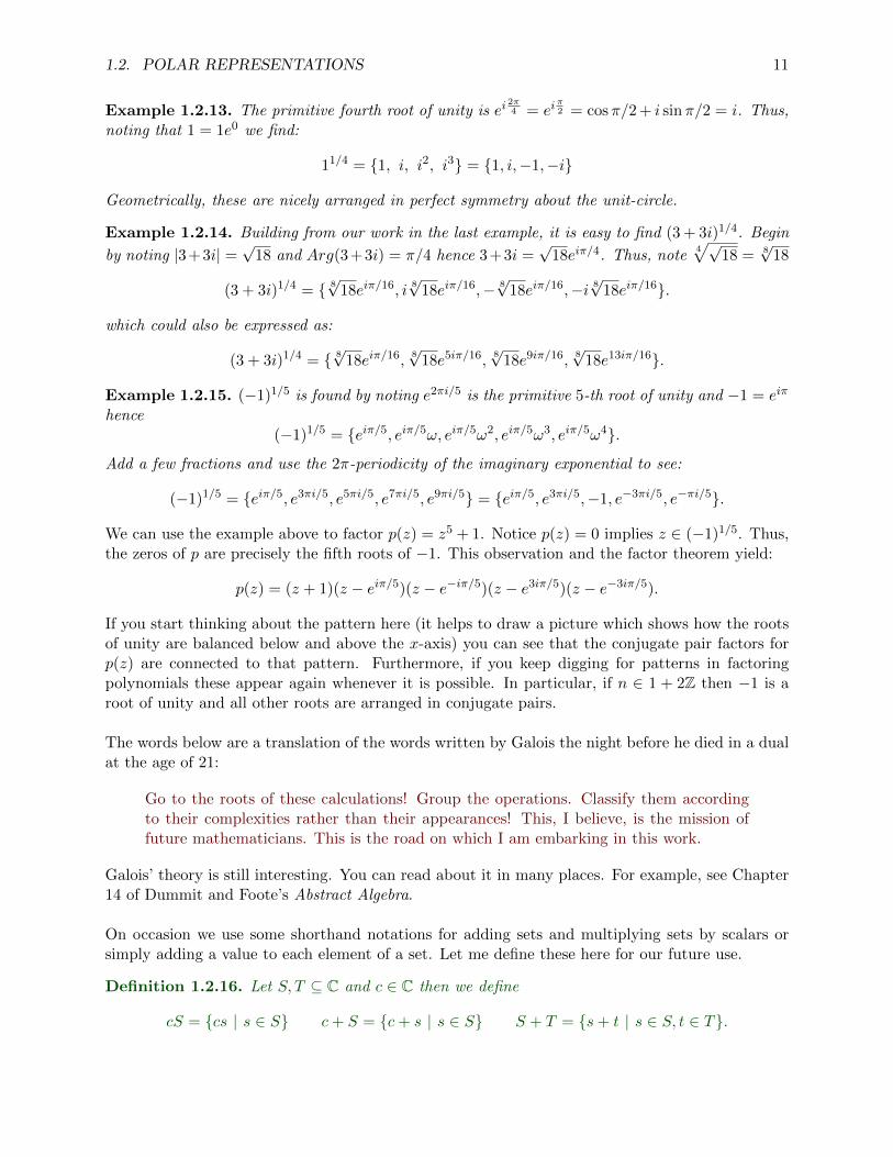
1.2. POLAR REPRESENTATIONS 11
Example 1.2.13. The primitive fourth root of unity is ei2π4 = ei
π2 = cosπ/2 + i sinπ/2 = i. Thus,
noting that 1 = 1e0 we find:
11/4 = {1, i, i2, i3} = {1, i,−1,−i}
Geometrically, these are nicely arranged in perfect symmetry about the unit-circle.
Example 1.2.14. Building from our work in the last example, it is easy to find (3 + 3i)1/4. Begin
by noting |3+3i| =√
18 and Arg(3+3i) = π/4 hence 3+3i =√
18eiπ/4. Thus, note4√√
18 = 8√
18
(3 + 3i)1/4 = { 8√
18eiπ/16, i8√
18eiπ/16,− 8√
18eiπ/16,−i 8√
18eiπ/16}.
which could also be expressed as:
(3 + 3i)1/4 = { 8√
18eiπ/16,8√
18e5iπ/16,8√
18e9iπ/16,8√
18e13iπ/16}.
Example 1.2.15. (−1)1/5 is found by noting e2πi/5 is the primitive 5-th root of unity and −1 = eiπ
hence(−1)1/5 = {eiπ/5, eiπ/5ω, eiπ/5ω2, eiπ/5ω3, eiπ/5ω4}.
Add a few fractions and use the 2π-periodicity of the imaginary exponential to see:
(−1)1/5 = {eiπ/5, e3πi/5, e5πi/5, e7πi/5, e9πi/5} = {eiπ/5, e3πi/5,−1, e−3πi/5, e−πi/5}.
We can use the example above to factor p(z) = z5 + 1. Notice p(z) = 0 implies z ∈ (−1)1/5. Thus,the zeros of p are precisely the fifth roots of −1. This observation and the factor theorem yield:
p(z) = (z + 1)(z − eiπ/5)(z − e−iπ/5)(z − e3iπ/5)(z − e−3iπ/5).
If you start thinking about the pattern here (it helps to draw a picture which shows how the rootsof unity are balanced below and above the x-axis) you can see that the conjugate pair factors forp(z) are connected to that pattern. Furthermore, if you keep digging for patterns in factoringpolynomials these appear again whenever it is possible. In particular, if n ∈ 1 + 2Z then −1 is aroot of unity and all other roots are arranged in conjugate pairs.
The words below are a translation of the words written by Galois the night before he died in a dualat the age of 21:
Go to the roots of these calculations! Group the operations. Classify them accordingto their complexities rather than their appearances! This, I believe, is the mission offuture mathematicians. This is the road on which I am embarking in this work.
Galois’ theory is still interesting. You can read about it in many places. For example, see Chapter14 of Dummit and Foote’s Abstract Algebra.
On occasion we use some shorthand notations for adding sets and multiplying sets by scalars orsimply adding a value to each element of a set. Let me define these here for our future use.
Definition 1.2.16. Let S, T ⊆ C and c ∈ C then we define
cS = {cs | s ∈ S} c+ S = {c+ s | s ∈ S} S + T = {s+ t | s ∈ S, t ∈ T}.
12 CHAPTER I. THE COMPLEX PLANE AND ELEMENTARY FUNCTIONS
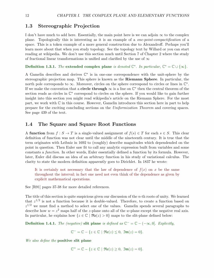
1.3 Stereographic Projection
I don’t have much to add here. Essentially, the main point here is we can adjoin ∞ to the complexplane. Topologically this is interesting as it is an example of a one-point-compactification of aspace. This is a token example of a more general construction due to Alexandroff. Perhaps you’lllearn more about that when you study topology. See the topology text by Willard or you can startreading at wikipedia. We don’t use this section much until Section 7 of Chapter 2 where the studyof fractional linear transformations is unified and clarified by the use of ∞
Definition 1.3.1. The extended complex plane is denoted C∗. In particular, C∗ = C ∪ {∞}.
A Gamelin describes and derives C∗ is in one-one correspondence with the unit-sphere by thestereographic projection map. This sphere is known as the Riemann Sphere. In particular, thenorth pole corresponds to ∞. Moreover, circles on the sphere correspond to circles or lines in C∗.If we make the convention that a circle through ∞ is a line on C∗ then the central theorem of thesection reads as circles in C∗ correspond to circles on the sphere. If you would like to gain furtherinsight into this section you might read wikipedia’s article on the Riemann Sphere. For the mostpart, we work with C in this course. However, Gamelin introduces this section here in part to helpprepare for the exciting concluding sections on the Uniformization Theorem and covering spaces.See page 439 of the text.
1.4 The Square and Square Root Functions
A function from f : S → T is a single-valued assignment of f(s) ∈ T for each s ∈ S. This cleardefinition of function was not clear until the middle of the nineteenth century. It is true that theterm originates with Leibniz in 1692 to (roughly) describe magnitudes which dependended on thepoint in question. Then Euler saw fit to call any analytic expression built from variables and someconstants a function. In other words, Euler essentially defined a function by its formula. However,later, Euler did discuss an idea of an arbitrary function in his study of variational calculus. Theclarity to state the modern definition apparently goes to Dirichlet. In 1837 he wrote:
It is certainly not necessary that the law of dependence of f(x) on x be the samethroughout the interval; in fact one need not even think of the dependence as given byexplicit mathematical operations.
See [R91] pages 37-38 for more detailed references.
The title of this section is quite suspicious given our discussion of the n-th roots of unity. We learnedthat z1/2 is not a function because it is double-valued. Therefore, to create a function based onz1/2 we must find a method to select one of the values. Gamelin spends several paragraphs todescribe how w = z2 maps half of the z-plane onto all of the w-plane except the negative real axis.In particular, he explains how {z ∈ C | Re(z) > 0} maps to the slit-plane defined below:
Definition 1.4.1. The (negative) slit plane is defined as C− = C− (−∞, 0]. Explicitly,
C− = C− {z ∈ C | Re(z) ≤ 0, Im(z) = 0}.
We also define the positive slit plane
C+ = C− {z ∈ C | Re(z) ≥ 0, Im(z) = 0}.

1.4. THE SQUARE AND SQUARE ROOT FUNCTIONS 13
Generically, when a ray is removed from C the resulting object is called a slit-plane. We mostlyfind use of C− since it is tied to the principle argument function. Let us introduce some notationto sort out what is said in this section. Mostly we need function notation and the concept of arestriction.
Definition 1.4.2. Let S ⊆ C and f : S → C a function. If U ⊆ S then we define the restrictionof f to U to be the function f |U : U → C where f |U (z) = f(z) for all z ∈ U .
Often a function is not injective on its domain, but, if we make a suitable restriction of the domainthen an inverse function exists. In calculus I call this a local inverse of the function. In the contextof complex analysis, the process of restricting the domain such that the range of the restrictiondoes not multiply cover C is known as making a branch cut. The reason for that terminology ismanifest in the pictures on page 17 of Gamelin. In what follows I show how a different branch ofthe square root may be selected.
Example 1.4.3. Let f : C → C be defined by f(z) = z2. Suppose we wish to make a branch cutof z1/2 along [0,∞). This would mean we wish to delete the postive real axis from the range ofthe square function. Let us denote C+ = C − [0,∞). The deletion of [0,∞) means we need toeliminate z which map to the positive real axis. This suggests we limit the argument of z such thatArg(z2) 6= 0. In particular, let us define U = {z ∈ C | Im(z) > 0}. This is the upper half plane.Notice if z ∈ U then Arg(z) ∈ (0, π). That is, z ∈ U implies z = |z|eiθ for 0 < θ < π. Note:
f |U (z) = z2 =(|z|eiθ
)2= |z|2e2iθ
Observe 0 < 2θ < 2π hence Arg(z2) ∈ (−π, 0) ∪ (0, π]. To summarize, if z ∈ U and w = z2 thenw ∈ C+. Furthermore, we can provide a nice formula for f3 = (f |U )−1 : C+ → U . For ρeiφ ∈ C+
where 0 < φ < 2π,f3(ρeiφ) =
√ρeiφ/2.
We could also use the lower half-plane to map to C+. Let V = {z ∈ C | − π < Arg(z) < 0}and notice for z ∈ V we have z2 = |z|2e2iθ. Thus, once again the standard angle of w = z2 takeson all angles except θ = 0. This is awkwardly captured in terms of the principal argument asArg(w) ∈ (−π, 0) ∪ (0, π]. Define f4 = (f |V )−1 : C+ → V for ρeiφ ∈ C+ where 0 < φ < 2π by
f4(ρeiφ) = −√ρeiφ/2.
Together, the ranges of f3 and f4 cover almost the whole z-plane. You can envision how to drawpictures for f3 and f4 which are analogus to those given for the principal branch and its negative.
It is customary to use the notation√w for the principal branch. Likewise, for other root functions
the same convention is made:
Definition 1.4.4. The principal branch of the n-th root is defined by:
n√w = n
√|w|ei
Arg(w)n
for each w ∈ C×.
Notice that ( n√w)n =
(n√|w|ei
Arg(w)n
)n= |w|eiArg(w) = w. Therefore, f(z) = zn has a local inverse
function given by the principal branch. The range of the principal branch function gives the domainon which the principal branch serves as an inverse function. Since −π < Arg(w) < π for w ∈ C−
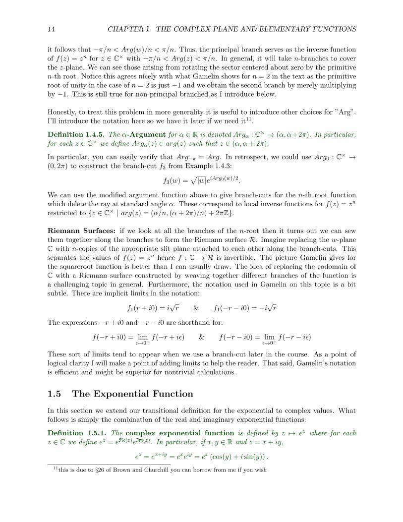
14 CHAPTER I. THE COMPLEX PLANE AND ELEMENTARY FUNCTIONS
it follows that −π/n < Arg(w)/n < π/n. Thus, the principal branch serves as the inverse functionof f(z) = zn for z ∈ C× with −π/n < Arg(z) < π/n. In general, it will take n-branches to coverthe z-plane. We can see those arising from rotating the sector centered about zero by the primitiven-th root. Notice this agrees nicely with what Gamelin shows for n = 2 in the text as the primitiveroot of unity in the case of n = 2 is just −1 and we obtain the second branch by merely multiplyingby −1. This is still true for non-principal branched as I introduce below.
Honestly, to treat this problem in more generality it is useful to introduce other choices for ”Arg”.I’ll introduce the notation here so we have it later if we need it11.
Definition 1.4.5. The α-Argument for α ∈ R is denoted Argα : C× → (α, α+2π). In particular,for each z ∈ C× we define Argα(z) ∈ arg(z) such that z ∈ (α, α+ 2π).
In particular, you can easily verify that Arg−π = Arg. In retrospect, we could use Arg0 : C× →(0, 2π) to construct the branch-cut f3 from Example 1.4.3:
f3(w) =√|w|eiArg0(w)/2.
We can use the modified argument function above to give branch-cuts for the n-th root functionwhich delete the ray at standard angle α. These correspond to local inverse functions for f(z) = zn
restricted to {z ∈ C× | arg(z) = (α/n, (α+ 2π)/n) + 2πZ}.
Riemann Surfaces: if we look at all the branches of the n-root then it turns out we can sewthem together along the branches to form the Riemann surface R. Imagine replacing the w-planeC with n-copies of the appropriate slit plane attached to each other along the branch-cuts. Thisseparates the values of f(z) = zn hence f : C → R is invertible. The picture Gamelin gives forthe squareroot function is better than I can usually draw. The idea of replacing the codomain ofC with a Riemann surface constructed by weaving together different branches of the function isa challenging topic in general. Furthermore, the notation used in Gamelin on this topic is a bitsubtle. There are implicit limits in the notation:
f1(r + i0) = i√r & f1(−r − i0) = −i
√r
The expressions −r + i0 and −r − i0 are shorthand for:
f(−r + i0) = limε→0+
f(−r + iε) & f(−r − i0) = limε→0+
f(−r − iε)
These sort of limits tend to appear when we use a branch-cut later in the course. As a point oflogical clarity I will make a point of adding limits to help the reader. That said, Gamelin’s notationis efficient and might be superior for nontrivial calculations.
1.5 The Exponential Function
In this section we extend our transitional definition for the exponential to complex values. Whatfollows is simply the combination of the real and imaginary exponential functions:
Definition 1.5.1. The complex exponential function is defined by z 7→ ez where for eachz ∈ C we define ez = eRe(z)eIm(z). In particular, if x, y ∈ R and z = x+ iy,
ez = ex+iy = exeiy = ex (cos(y) + i sin(y)) .
11this is due to §26 of Brown and Churchill you can borrow from me if you wish

1.5. THE EXPONENTIAL FUNCTION 15
When convenient, we also use the notation ez = exp(z) to make the argument of the exponentialmore readable. 12. Consider, as |eiy| =
√eiye−iy =
√e0 = 1 we find
|ez| = |exeiy| = |ex||eiy| = |ex| = ex.
The magnitude of the complex exponential is unbounded as x → ∞ whereas the magnitude ap-proaches zero as x→ −∞. The argument of ez is immediate from the definition; Arg(ez) = Arg(z).I would not write arg(ez) = y as Gamelin writes on page 19 as arg(z) is a set of values whereas yis a value. It’s not hard to fix, we just say if z = x+ iy then arg(ex+iy) = {y + 2πk | k ∈ Z}. Thiscan be glibly written as arg(ez) = arg(z).
Observe domain(ez) = C however range(ez) = C× as we know eiy 6= 0 for all y ∈ R. Furthermore,the complex exponential is not injective precisely because the imaginary exponential is not injective.If two complex exponentials agree then their arguments need not be equal. In fact:
ez = ew ⇔ z − w ∈ 2πiZ.
Moreover, ez = 1 iff z = 2πik for some k ∈ Z. As Gamelin points out, we have 2πi-periodicity ofthe complex exponential function; ez+2πi = ez. We also have
ez+w = ezew & (ez)−1 = 1/ez = e−z.
The proof of the addition rule above follows from the usual laws of exponents for the real exponentialfunction as well as the addition rules for cosine and sine which give the addition rule for imaginaryexponentials. Of course, eze−z = ez−z = e0 = 1 shows 1/ez = e−z but it is also fun to work it outfrom our previous formula for the reciprocal 1/z = z/|z|2. We showed |ex+iy| = ex hence:
1
ez=exe−iy
(ex)2= e−xe−iy = e−(x+iy) = e−z.
As is often the case, the use of x, y notation clutters the argument.
To understand the geometry of z 7→ ez we study how the exponential maps the z-plane to thew = u+ iv-plane where w = ez. Often we look at how lines or circles transform. In this case, lineswork well. I’ll break into cases to help organize the thought:
1. A vertical line in the z = x + iy-plane has equation x = xo whereas y is free to rangeover R. Consider, exo+iy = exoeiy. As y-varies we trace out a circle of radius exo in thew = u+ iv-plane. In particular, it has equation u2 + v2 = (exo)2.
2. A horizontal line in the z = x + iy-plane has equation y = yo whereas x is free to rangeover R. Consider, ex+iyo = exeiyo . As x-varies we trace out a ray at standard angle yo in thew-plane.
If you put these together, we see a little rectangle [a, b]× [c, d] in the z-plane transforms to a littlesector in the w-plane with |w| ∈ [ea, eb] and Arg(w) ∈ [c, d] (assuming [c, d] ⊆ (−π, π] otherwisewe’d have to deal with some alternate argument function). See Figure 5.3 at this website.
12 Notice, we have not given a careful definition of ex here for x ∈ R. We assume, for now, the reader has somebase knowledge from calculus which makes the exponential function at least partly rigorous. Later in this our studywe find a definition for the exponential which supercedes the one given here and provides a rigorous underpinning forall these fun facts

16 CHAPTER I. THE COMPLEX PLANE AND ELEMENTARY FUNCTIONS
1.6 The Logarithm Function
As we discussed in the previous section, the exponential function is not injective. In particular,ez = ez+2πi hence as we study z 7→ w = ez we find each horizontal strip R × (yo, y + 2π) maps toC×−{w ∈ C | arg(w)∩{yo}. In other words, we map horizontal strips of height 2π to the slit-planewhere the slit is at standard angle yo. To cover C− we map the horizontal strip R× (−π, π) to C−.This gives us the principal logarithm
Definition 1.6.1. The principal logarithm is defined by Log(z) = ln(|z|) + iArg(z) for eachz ∈ C×. In particular, for z = x+ iy with −π < y ≤ π we define:
Log(x+ iy) = ln√x2 + y2 + iy.
We can also simplify the formula by the power property of the real logarithm to
Log(x+ iy) =1
2ln(x2 + y2) + iy.
Notice: we use ”ln” for the real logarithm function. In contrast, we reserve the notations ”log”and ”Log” for complex arguments. Please do not write ln(1 + i) as in our formalism that is justnonsense. There is a multiply-valued function of which this is just one branch. In particular:
Definition 1.6.2. The logarithm is defined by log(z) = ln(|z|) + iarg(z) for each z ∈ C×. Inparticular, for z = x+ iy 6= 0
log(x+ iy) = {ln√x2 + y2 + iy | x+ iy ∈ C×}.
Example 1.6.3. To calculate Log(1 + i) we change to polar form 1 + i =√
2eiπ/4. Thus
Log(1 + i) = ln√
2 + iπ/4.
Note arg(1 + i) = π/4 + 2πZ hence
log(1 + i) = ln√
2 + iπ/4 + 2πiZ.
There are many values of the logarithm of 1 + i. For example, ln√
2 + 9iπ/4 and ln√
2 − 7iπ/4are also a logarithms of 1 + i. These are the are the beginnings of the two tails13 which Gamelinillustrates on page 22.
We could use Argα as given in Definition 1.4.5 to define other branches of the logarithm. Inparticular, a reasonable notation would be:
Logα(z) = ln |z|+ iArgα(z).
Once more, α = −π gives the principal case; Log−π = Log. The set of values in log(z) is formedfrom the union of all possible values for Logα(z) as we vary α over R. In Gamelin he considers.
fm(z) = Log(z) + 2πim
for m ∈ Z. To translate to the α-notation, m = 0 gives α = −π, m = 1 gives α = π, generally mcorresponds to α = −π + 2πm. The distinction is not particularly interesting, basically, Gamelin
13 I can’t help but wonder, is there a math with more tails
1.7. POWER FUNCTIONS AND PHASE FACTORS 17
has simply made a choice to put the branch-cut on the negative real axis.
Finally, let us examine how the logarthim does provide an inverse for the exponential. If werestrict to a particular branch then the calculation is simple. For example, the principal branch,let z ∈ R× (−π, π) and consider
eLog(z) = eln |z|+iArg(z) = eln |z|eiArg(z) = |z|eiArg(z) = z.
Conversely, for z ∈ C−,
Log(ez) = ln |ez|+ iArg(ez) = ln(eRe(z)) + iIm(z) = Re(z) + iIm(z) = z.
The discussion for the multiply valued logarithm requires a bit more care. Let z ∈ C×, by definition,
log(z) = {ln |z|+ i(Arg(z) + 2πk) | k ∈ Z}.
Let w ∈ log(z) and consider,
ew = exp (ln |z|+ i(Arg(z) + 2πk))
= exp (ln |z|+ i(Arg(z))
= exp(ln |z|)exp(i(Arg(z))
= |z|eiArg(z)
= z.
It follows that elog(z) = {z}. Sometimes, you see this written as elog(z) = z. if the author is not com-mitted to viewing log(z) as a set of values. I prefer to use set notation as it is very tempting to usefunction-theoretic thinking for multiply-valued expressions. For example, a dangerous calculation:
1 = −i2 = −ii = −(−1)1/2(−1)1/2 = −((−1)(−1))1/2 = −(1)1/2 = −1.
Wait. This is troubling if we fail to appreciate that 11/2 = {1,−1}. What appears as equality formultiply-valued functions is better understood in terms of inclusion in a set. I will try to be explicitabout sets when I use them, but, beware, Gamelin does not share my passion for pedantics.
The trouble arises when we ignore the fact there are multiple values for a complex power functionand we try to assume it ought to behave as an honest, single-valued, function. See Problem 12 foran opportunity to think about this a bit more.
1.7 Power Functions and Phase Factors
Definition 1.7.1. Let z, α ∈ C with z 6= 0. Define zα to be the set of values zα = exp(αlog(z)).
In particular,zα = {exp(α[Log(z) + 2πik]) | k ∈ Z}.
However,exp(α[Log(z) + 2πik]) = exp(α[Log(z))exp(2απik).
We have already studied the case α = 1/n. In that case exp(2απik) = exp(2απi/n) are the n-roots of unity. In the case α ∈ Z the phase factor exp(2απik) = 1 and z 7→ zα is single-valuedwith domain C. Generally, the complex power function is not single-valued unless we make somerestriction on the domain.

18 CHAPTER I. THE COMPLEX PLANE AND ELEMENTARY FUNCTIONS
Example 1.7.2. Observe that log(3) = ln(3) + 2πiZ hence:
3i = ei log(3) = ei(ln(3)+2πiZ) = ei ln(3)e−2πZ.
In other words,
3i = [cos(ln(3)) + i sin(ln(3))]e−2πZ
= {[cos(ln(3)) + i sin(ln(3))]e−2πk | k ∈ Z}.
In this example, the values fall along the ray at θ = ln(3). As k →∞ the values approach the originwhereas as k → −∞ the go off to infinity. I suppose we could think of it as two tails, one stretchedto ∞ and the other bunched at 0.
On page 25 Gamelin shows a similar result for ii. However, as was known to Euler [R91] (p. 162),there is a real value of ii. In a letter to Goldbach in 1746, Euler wrote:
Recently I have found that the expression (√−1)
√−1 has a real value, which in decimal
fraction form = 0.2078795763; this seems remarkable to me.
On pages 160-165 of [R91] a nice discussion of the general concept of a logarithm is given. Theproblem of multiple values is dealt with directly with considerable rigor.
Concerning phase factors: Suppose we choose a particular value for α ∈ C− Z then the phasefactor in zα is nontrivial and it is the case that zα is a set with infinitely many values. If we selectone of the values, say fk(z) and allow z to vary then there will be points where the output of fk(z)is discontinuous. In particular, as
zα = {exp(α[Log(z) + 2πik]) | k ∈ Z}.
we may choose the value for fixed k ∈ Z as:
fk(z) = eαLog(z)e2πik
The domain of fk is C− since we wrote the formula using the principal logarithm. We would liketo compare the values of fk(z) as the approach the slit in C− from below and above. From above,we have z = |z|eiθ for θ → π−. This gives,
fk(|z|eiθ) = eα(ln |z|+iθ)e2πik
and I think we can agree (using c = eα(ln |z|)e2πik for the rightmost equality)
limθ→π−
fk(|z|eiπ) = eα(ln |z|+iπ)e2πik = ceiαπ
On the other hand, approaching the slit from below,
limθ→−π+
fk(|z|eiπ) = eα(ln |z|−iπ)e2πik = ce−iαπ.
If we envision beginning at the lower edge of the slit with value ce−iαπ and we travel around a CCWcircle until we reach the upper edge of the slit with value ceiαπ we see the initial value is multipliedby the phase factor e2πiα as it traverses the circle. The analysis on page 25 of Gamelin reveals thesame for a power function built with Argo(z). In that case, we see again the phase factor of e2πiα
arise as we traverse a circle in the CCW14 direction which begins at θ = 0 and ends at θ = 2π.
14Gamelin calls this the positive direction and I call the same direction by Counter-Clock-Wise by CCW.

1.8. TRIGONOMETRIC AND HYPERBOLIC FUNCTIONS 19
Theorem 1.7.3. Phase change lemma: let g(z) be a (single-valued) function that is definedand continuous near zo. For any continuously varying branch of (z − zo)
α the function f(z) =(z − zo)αg(z) is multiplied by the phase factor e2πiα when z traverses a complete circle about zo inthe CCW fashion.
For example, if we have zo = 0 and g(z) = 1 and α = 1/2 then the principal root function f(z) =√z
jumps by e2πi/2 = −1 as we cross the slit (−∞, 0]. The connection between the phase change lemmaand the construction of Riemann surfaces is an interesting topic which we might return to later iftime permits. However, for the moment we just need to be aware of the subtle points in definingcomplex power functions.
1.8 Trigonometric and Hyperbolic Functions
If you’ve taken calculus with me then you already know that for θ ∈ R the formulas:
cos θ =1
2
(eiθ + e−iθ
)& sin θ =
1
2i
(eiθ − e−iθ
)are of tremendous utility in the derivation of trigonometric identities. They also set the stage forour definitions of sine and cosine on C:
Definition 1.8.1. Let z ∈ C. We define:
cos z =1
2
(eiz + e−iz
)& sin z =
1
2i
(eiz − e−iz
)All your favorite algebraic identities from real trigonometry hold here, unless, you are a fan of| sin(x)| ≤ 1 and | cos(x)| ≤ 1. Those are not true for the complex sine and cosine. In particular,note:
ei(x+iy) = eixe−y & e−i(x+iy) = e−ixey
Hence,
cos(x+ iy) =1
2
(eixe−y + e−ixey
)&
1
2i
(eixe−y − e−ixey
)Clearly as |y| → ∞ the moduli of sine and cosine diverge. I present explicit formulas for the moduliof sine and cosine later in terms of the hyperbolic functions.
I usually introduce hyperbolic cosine and sine as the even and odd parts of the exponential function:
ex =1
2
(ex + e−x
)︸ ︷︷ ︸
cosh(x)
+1
2
(ex − e−x
)︸ ︷︷ ︸
sinh(x)
.
Once again, the complex hyperbolic functions are merely defined by replacing the real variable xwith the complex variable z:
Definition 1.8.2. Let z ∈ C. We define:
cosh z =1
2
(ez + e−z
)& sinh z =
1
2
(ez − e−z
).

20 CHAPTER I. THE COMPLEX PLANE AND ELEMENTARY FUNCTIONS
The hyperbolic trigonometric functions and the circular trigonometric functions are linked by thefollowing simple identities:
cosh(iz) = cos(z) & sinh(iz) = i sin(z)
and
cos(iz) = cosh(z) & sin(iz) = i sinh(z).
Return once more to cosine and use the adding angle formula (which holds in the complex domainas the reader is invited to verify)
cos(x+ iy) = cos(x) cos(iy)− sin(x) sin(iy) = cos(x) cosh(y)− i sin(x) sinh(y)
and
sin(x+ iy) = sin(x) cos(iy) + cos(x) sin(iy) = sin(x) cosh(y) + i cos(x) sinh(y).
In view of these identities, we calculate the modulus of sine and cosine directly,
| cos(x+ iy)|2 = cos2(x) cosh2(y) + sin2(x) sinh2(y)
| sin(x+ iy)|2 = sin2(x) cosh2(y) + cos2(x) sinh2(y).
However, cosh2 y − sinh2 y = 1 hence
cos2(x) cosh2(y) + sin2(x) sinh2(y) = cos2(x)[1 + sinh2(y)] + sin2(x) sinh2(y)
= cos2(x) + [cos2(x) + sin2(x)] sinh2(y)
= cos2(x) + sinh2(y).
A similar calculation holds for | sin(x+ iy)|2 and we obtain:
| cos(x+ iy)|2 = cos2(x) + sinh2(y) & | sin(x+ iy)|2 = sin2(x) + sinh2(y).
Notice, for y ∈ R, sinh(y) = 0 iff y = 0. Therefore, the only way the moduli of sine and cosine canbe zero is if y = 0. It follows that only zeros of sine and cosine are precisely those with which weare already familar on R. In particular,
sin(πZ) = {0} & cos
(2Z + 1
2π
)= {0}.
There are pages and pages of interesting identities to derive for the functions introduced here.However, I resist. In part because they make nice homework/test questions for the students. But,also, in part because a slick result we derive later on forces identities on R of a particular type tonecessarily extend to C. More on that in Chapter 5 of Gamelin.
Definition 1.8.3. Tangent and hyperbolic tangent are defined in the natural manner:
tan z =sin z
cos z& tanh z =
sinh z
cosh z.
The domains of tangent and hyperbolic tangent are simply C with the zeros of the denominatorfunction deleted. In the case of tangent, domain(tan z) = C−
(2Z+1
2
)π.

1.8. TRIGONOMETRIC AND HYPERBOLIC FUNCTIONS 21
Inverse Trigonometric Functions: consider f(z) = sin z then as sin(z + 2πk) = sin(z) for allk ∈ Z we see that the inverse of sine is multiply-valued. If we wish to pick one of those values weshould study how to solve w = sin z for z. Note:
2iw = eiz − e−iz
multiply by eiz to obtain:2iweiz = (eiz)2 − 1.
Now, substitute η = eiz to obtain:
2iwη = η2 − 1 ⇒ 0 = η2 − 2iwη − 1.
Completing the square yields,
0 = (η − iw)2 + w2 − 1 ⇒ (η − iw)2 = 1− w2.
Consequently, η− iw ∈ (1−w2)1/2 which in terms of the principal root implies η = iw±√
1− w2.But, η = eiz so we find:
eiz = iw ±√
1− w2.
There are many solutions to the equation above which are by custom included in the multiply-valuesinverse sine mapping below:
z = sin−1(w) = −i log(iw ±√
1− w2).
Gamelin describes how to select a particular branch in terms of the principal logarithm.

22 CHAPTER I. THE COMPLEX PLANE AND ELEMENTARY FUNCTIONS

Chapter II
Analytic Functions
What is analysis? I sometimes glibly say something along the lines of: algebra is about equationswhereas analysis is about inequality. Of course, any one-liner cannot hope to capture the entiretyof a field of mathematics. We can certainly say both analysis and algebra are about structure.In algebra, the type of structure tends to be about generalizing rules of arithmetic. In analysis,the purpose of the structure is to generalize the process of making imprecise statements preciselyknown. For example, we might say a function is continuous if its values don’t jump for nearbyinputs. But, the structure of the limit replaces this fuzzy idea with a precise framework to judgecontinuity. Remmert remarks on page 38 of [R91] that the idea of continuity pre-rigorization is notstrictly in one-one correspondence to our modern usage of the term. Sometimes, the term continu-ous implied analyticity of the function. We will soon appreciate that analyticity1 is a considerablystronger condition. The process of clarifying definitions is not always immediate. Cauchy’s impre-cise language captured the idea of the limit, but, it is generally agreed that it was not until thework of Weierstrauss (and his introduction of the dreaded εδ-notation which haunts students tothe present day) that the limit was precisely defined. There are further refinements of the limitconcept in topology which supercede the results given for sequences in this chapter. I can suggestfurther reading if you have interest.
Beware, this review of real analysis is likely more of an introduction than a review. Just try toget an intuitive appreciation of the definitions which are covered and remember when a homeworkproblem looks trivial it probably requires you to do hand-to-hand combat through one of thesedefinitions. I’m here to help if you’re lost.
2.1 Review of Basic Analysis
A function n 7→ an from N to C is a sequence of complex numbers. Sometimes we think ofa sequence as an ordered list; {an} = {a1, a2, . . . }. We assume the domain of sequences in thissection is N but this is not an essential constraint, we could just as well study sequences withdomain {k, k + 1, . . . } for some k ∈ Z.
Definition 2.1.1. Sequential Limit: Let an be a complex sequence and a ∈ C. We say an → aiff for each ε > 0 there exists N ∈ N such that |an − a| < ε whenever n > N . In this case we write
limn→∞
an = a.
1I try to use the term holomorphic in contrast to Gamelin
23

24 CHAPTER II. ANALYTIC FUNCTIONS
Essentially, the idea is that the sequence clusters around L as we go far out in the list.
Definition 2.1.2. Bounded Sequence: Suppose R > 0 and |an| < R for all n ∈ N then {an} isa bounded sequence
The condition |an| < R implies an is in the disk of radius R centered at the origin.
Theorem 2.1.3. Convergent Sequence Properties: A convergent sequence is bounded. Fur-thermore, if sn → s and tn → t then
(a.) sn + tn → s+ t
(b.) sntn → st
(c.) sn/tn → s/t provided t 6= 0.
The proof of the theorem above mirrors the proof you would give for real sequences.
Theorem 2.1.4. in-between theorem: If rn ≤ sn ≤ tn, and if rn → L and tn → L then sn → L.
The theorem above is for real sequences. We have no2 order relations on C. Recall, by definition,monotonic sequences sn are either always decreasing (sn+1 ≤ sn) or always increasing (sn+1 ≥ sn).The completeness, roughly the idea that R has no holes, is captured by the following theorem:
Theorem 2.1.5. A bounded monotone sequence of real numbers coverges.
The existence of a limit can be captured by the limit inferior and the limit superior. These are inturn defined in terms of subsequences.
Definition 2.1.6. Let {an} be a sequence. We define a subsequence of {an} to be a sequence ofthe form {anj} where j 7→ nj ∈ N is a strictly increasing function of j.
Standard examples of subsequences of {aj} are given by {a2j} or {a2j−1}.
Example 2.1.7. If aj = (−1)j then a2j = 1 whereas a2j−1 = −1. In this example, the evensubsequence and the odd sequence both converge. However, lim aj does not exist.
Apparently, considering just one subsequence is insufficient to gain much insight. On the otherhand, if we consider all possible subsequences then it is possible to say something definitive.
Definition 2.1.8. Let {an} be a sequence. We define limsup(an) to be the upper bound of allpossible subsequential limits. That is, if {anj} is a subsequence which converges to t (we allowt = ∞) then t ≤ limsup(an). Likewise, we define liminf(an) to be the lower bound (possibly −∞)of all possible subsequential limits of {an}.
Theorem 2.1.9. The sequence an → L ∈ R if and only iff limsup(an) = liminf(an) = L ∈ R.
The concepts above are not available directly on C as there is no clear definition of an increasingor decreasing complex number. However, we do have many other theorems for complex sequenceswhich we had before for R. In the context of advanced calculus, I call the following the vector limittheorem. It says: the limit of a vector-valued sequence is the vector of the limits of the componentsequences. Here we just have two components, the real part and the imaginary part.
2to be fair, you can order C, but the order is not consistent with the algebraic structure. See this answer

2.1. REVIEW OF BASIC ANALYSIS 25
Theorem 2.1.10. Suppose zn = xn + iyn ∈ C for all n ∈ N and z = x + iy ∈ C. The sequencezn → z if and only iff both xn → x and yn → y.
Proof Sketch: Notice that if xn → x and yn → y then it is an immediate consequence of Theorem2.1.3 that xn + iyn → x + iy. Conversely, suppose zn = xn + iyn → z. We wish to prove thatxn → x = Re(z) and yn → y = Im(z). The inequalities below are crucial:
|xn − x| ≤ |zn − z| & |yn − y| ≤ |zn − z|
Let ε > 0. Since zn → z we are free to select N ∈ N such that for n ≥ N we have |zn− z| < ε. But,then it follows |xn−x| < ε and |yn−y| < ε by the crucial inequalities. Hence xn → x and yn → y. �
Definition 2.1.11. We say a sequence {an} is Cauchy if for each ε > 0 there exists N ∈ N forwhich N < m < n implies |am − an| < ε.
As Gamelin explains, a Cauchy sequence is one where the differences am − an tend to zero in thetail of the sequence. At first glance, this hardly seems like an improvement on the definition ofconvergence, yet, in practice, so many proofs elegantly filter through the Cauchy criterion. In anyspace, if a sequence converges then it is Cauchy. However, the converse only holds for special spaceswhich are called complete.
Definition 2.1.12. A space is complete if every Cauchy sequence converges.
The content of the theorem below is that C is complete.
Theorem 2.1.13. A complex sequence converges iff it is a Cauchy sequence.
Real numbers as also complete. This is an essential difference between the rational and the realnumbers. There are certainly sequences of rational numbers whose limit is irrational. For example,the sequence of partial sums from the p = 2 series {1, 1 + 1/4, 1 + 1/4 + 1/9, . . . } has rationalelements yet limits to π2/6. This was shown by Euler in 1734 as is discussed on page 333 of [R91].The process of adjoining all limits of Cauchy sequences to a space is known as completing aspace. In particular, the completion of Q is R. Ideally, you will obtain a deeper appreciation ofCauchy sequences and completion when you study real analysis. That said, if you are willing toaccept the truth that R is complete it is not much more trouble to show Rn is complete. I plan toguide you through the proof for C in your homework (see Problem 24).
Analysis with sequences is discussed at length in our real analysis course. On the other hand, whatfollows is the natural extsension of the (εδ)-definition to our current context3. In what follows weassume f : dom(f) ⊆ C→ C is a function and L ∈ C.
Definition 2.1.14. We say limz→zo
f(z) = L if for each ε > 0 there exists δ > 0 such that z ∈ C with
0 < |z − zo| < δ implies |f(z)− L| < ε.
We also write f(z)→ L as z → zo when the limit exists.
Theorem 2.1.15. Suppose limz→zo
f(z), limz→zo
g(z) ∈ C then
(a.) limz→zo
[f(z) + g(z)] = limz→zo
f(z) + limz→zo
g(z)
3in fact, we can also give this definition in a vector space with a norm, if such a space is complete then we call ita Banach space
26 CHAPTER II. ANALYTIC FUNCTIONS
(b.) limz→zo
[f(z)g(z)] = limz→zo
f(z) · limz→zo
g(z)
(c.) limz→zo
[cf(z)] = c limz→zo
f(z)
(d.) limz→zo
[f(z)
g(z)
]=
limz→zo f(z)
limz→zo g(z)
where in the last property we assume limz→zo
g(z) 6= 0.
Once more, the proof of this theorem mirrors the proof which was given in the calculus of R. Onesimply replaces absolute value with modulus and the same arguments go through. If you wouldlike to see explicit arguments you can take a look at my calculus I lecture notes (for free !). Theother way to prove these is to use Lemma 2.1.17 and apply it to Theorem 2.1.3.
Definition 2.1.16. If f : dom(f) ⊆ C→ C is a function zo ∈ dom(f) such that limz→zo
f(z) = f(zo)
then f is continuous at zo. Iif f is continuous at each point in U ⊆ dom(f) then we say f iscontinuous on U. When f is continuous on dom(f) we say f is continuous. The set of allcontinuous functions on U ⊆ C is denoted C0(U).
The definition above gives continuity at a point, continuity on a set and finally continuitiy of thefunction itself. In view of Theorem 2.1.15 we may immediately conclude that if f, g are continuousthen f+g, fg, cf and f/g are continuous provided g 6= 0. The conclusion holds at a point, on a com-mon subset of the domains of f, g and finally on the domains of the new functions f+g, fg, cf, f/g.
The lemma below connects the sequential and εδ-definitions of the limit. In words, if every sequencezn converging to zo gives sequences of values f(zn) converging to L then f(z)→ L as z → zo.
Lemma 2.1.17. limz→zo
f(z) = L iff whenever zn → zo it implies f(zn)→ L.
Proof: this is a biconditional claim. I’ll to prove half of the lemma. You can prove the interestingpart for some bonus points.
(⇒) Suppose limz→zo
f(z) = L. Also, let zn be a sequence of complex numbers which converges to
zo. Let ε > 0. Notice, as f(z) → L we may choose δε > 0 for which 0 < |z − zo| < δε im-plies |f(z) − L| < ε. Furthemore, as zn → zo we can choose Mδε ∈ N such that n > Mδε implies|zn−zo| < δε. Finally, consider if n > Mδε then |zn−zo| < δε hence |f(zn)−L| < ε. Thus f(zn)→ L.
(⇐) left to reader. See this answer to the corresponding question in the real case. �
The paragraph on page 37 repeated below is very important to the remainder of the text. Heoften uses this simple principle to avoid writing a complete (and obvious) proof. His refusal towrite the full proof is typical of analysts’ practice. In fact, this textbook was recommended tome by a research mathematician whose work is primarily analytic. Rigor should not be mistakenfor the only true path. It is merely the path we teach you before you are ready for other moreintuitive paths. You might read Terry Tao’s excellent article on the different postures we strike asour mathematical education progresses. See There’s more to mathematics than rigour and proofsfrom Tao’s blog. From page 36 of Gamelin,
”A useful strategy for showing that f(z) is continuous at zo is to obtain an estimate ofthe form |f(z)−f(zo)| ≤ C|z−zo| for z near zo. This guarantees that |f(z)−f(zo)| < εwhenever |z− zo| < ε/C, so that we can take δ = ε/C in the formal definition of limit”

2.1. REVIEW OF BASIC ANALYSIS 27
It is also worth repeating Gamelin’s follow-up example here:
Example 2.1.18. The inequalities
|Re(z − zo)| ≤ |z − zo|, |Im(z − zo)| ≤ |z − zo|, & ||z| − |zo|| ≤ |z − zo|indicate that Re, Im and modulus are continuous at zo.
At this point we turn to the geometric topology of the plane. Fundamental to almost everything isthe idea of a disk
Definition 2.1.19. An open disk of radius ε centered at zo ∈ C is the subset all complex numberswhich are less than an ε distance from zo, we denote this open ball by
Dε(zo) = {z ∈ C | |z − zo| < ε}.The deleted-disk with radius ε centered at zo is likewise defined
Doε (zo) = {z ∈ C | 0 < |z − zo| < ε}.
The closed disk of radius ε centered at zo ∈ C is defined by
Dε(zo) = {z ∈ C | |z − zo| ≤ ε}.We use disks to define topological concepts in C.
Definition 2.1.20. Let S ⊆ C. We say y ∈ S is an interior point of S iff there exists some opendisk centered at y which is completely contained in S. If each point in S is an interior point thenwe say S is an open set.
Roughly, an open set is one with fuzzy edges. A closed set has solid edges. Furthermore, an openset is the same as its interior and closed set is the same as its closure.
Definition 2.1.21. We say y ∈ C is a limit point of S iff every open disk centered at y containspoints in S − {y}. We say y ∈ C is a boundary point of S iff every open disk centered at ycontains points not in S and other points which are in S − {y}. We say y ∈ S is an isolatedpoint or exterior point of S if there exist open disks about y which do not contain other points inS. The set of all interior points of S is called the interior of S. Likewise the set of all boundarypoints for S is called the boundary of S and is denoted ∂S. The closure of S is defined to beS = S ∪ {y ∈ C | y a limit point of S}.To avoid certain pathological cases we often insist that the set considered is a domain or a region.These are technical terms in this context and we should be careful not to confuse them with theirprevious uses in mathematical discussion.
Definition 2.1.22. If a, b ∈ C then we define the directed line segment from a to b by
[a, b] = {a+ t(b− a) | t ∈ [0, 1]}This notation is pretty slick as it agrees with interval notation on R when we think about them asline segments along the real axis of the complex plane. However, certain things I might have calledcrazy in precalculus now become totally sane. For example, [4, 3] has a precise meaning. I think,to be fair, if you teach precalculus and someone tells you that [4, 3] meant the same set of points,but they prefer to look at them Manga-style then you have to give them credit.
Definition 2.1.23. A subset U of the complex plane is called star shaped with star center zoif there exists zo such that each z ∈ U has [zo, z] ⊆ U .
A given set may have many star centers4. For example, C− is star shaped and the only star centers
4if a person knew something about this activity called basketball there must be team-specific jokes to make here

28 CHAPTER II. ANALYTIC FUNCTIONS
are found on [0,∞). Likewise, C+ is star shaped with possible star centers found on (−∞, 0].
Definition 2.1.24. A polygonal path γ from a to b in C is the union of finitely many linesegments which are placed end to end; γ = [a, z1] ∪ [z1, z2] ∪ · · · ∪ [zn−2, zn−1] ∪ [zn−1, b].
Gamelin calls a polygonal path a broken line segment.
Definition 2.1.25. A set S ⊆ C is connected iff there exists a polygonal path contained in Sbetween any two points in S. That is for all a, b ∈ S there exists a polygonal path γ from a to bsuch that γ ⊆ S
Incidentally, the definitions just offered for C apply equally well to Rn if we generalize modulus toEuclidean distance between points.
Definition 2.1.26. An open connected set is called a domain. We say R is a region if R = D∪Swhere D is a domain D and S ⊆ ∂D.
The concept of a domain is most commonly found in the remainder of our study. You should takenote of its meaning as it will not be emphasized every time it is used later.
Definition 2.1.27. A subset U ⊆ C is bounded if there exists M > 0 and zo ∈ U for whichU ⊆ Dδ(zo). If U ⊆ C is both closed and bounded then we say U is compact.
I should mention the definition of compact given here is not a primary definition, when you studytopology or real analysis you will learn a more fundamental characterization of compactness. Wemay combine terms in reasonable ways. For example, a domain which is also star shaped is calleda star shaped domain. A region which is also compact is a compact region.
The theorem which follows is interesting because it connect a algebraic condition ∇h = 0 with atopological trait of connectedness. Recall that h : R2 → R is continuously differentiable if eachof the partial derivatives of h is continuous. We need this condition to avoid pathological issueswhich arise from merely assuming the partial derivatives exist. In the real case, the existence ofthe partial derivatives does not imply their continuity. We’ll see something different for C as westudy complex differentiability.
Theorem 2.1.28. If h(x, y) is a continuously differentiable function on a domain D such that
∇h =⟨∂h∂x ,
∂h∂y
⟩= 0 on D then h is constant.
Proof: Let p, q ∈ D. As D is connected there exists a polygonal path γ from p to q. Letp1, p2, . . . , pn be the points at which the line segments comprising γ are joined. In particular, γ1 isa path from p to p1 and we parametrize the path such that dom(γ1) = [0, 1]. By the chain rule,
d
dt(h(γ1(t))) = ∇h(γ1(t))) •
dγ1(t))
dt
however, γ1(t) ∈ D for each t hence ∇h(γ1(t))) = 0. Consequently,
d
dt(h(γ1(t))) = 0
It follows from calculus that h(γ1(0)) = h(γ1(1)) hence h(p) = h(p1). But, we can repeat thisargument to show h(p2) = h(p3) and so forth and we arrive at:
h(p) = h(p1) = h(p2) = · · · = h(pn) = h(q).
But, p, q were arbitrary thus h is constant on D. �

2.2. ANALYTIC FUNCTIONS 29
2.2 Analytic Functions
I do not really follow Gamelin here. We choose a different path, but, we begin the same:
Definition 2.2.1. If limz→zo
f(z)− f(zo)
z − zoexists then we say f is complex differentiable at zo
and we denote f ′ (zo) = limz→zo
f(z)− f(zo)
z − zo. Furthermore, the mapping z 7→ f ′(z) is the complex
derivative of f .
We continue to use many of the same notations as in first semester calculus. In particular,f ′(z) = df/dz and d/dz(f(z)) = f ′(z). My langauge differs slightly from Gamelin here in thatI insist we refer to the complex differentiability of f . There is also a concept of real differentiabilitywhich we compare, contrast and make good use of in the section after this section. If you lookat Definition 2.2.1 you should see that it is precisely the same definition as was given for R. Infact, most of the arguments we made for real derivatives of functions on R transfer to our currentcontext because the complex limit shares the same algebraic properties as the limit in R. I couldsimply go to my calculus I notes and cut and paste the relevant section here. All I would needto do for most arguments is just change x to z for the sake of style. That said, I’ll try to give adifferent argument here. The idea I’ll pursue is that we can prove most things about differentiationthrough the use of linearizations. To be careful, we’ll use the theorem of Caratheodory5 to makeour linearization arguments a bit more rigorous.
The central point is Caratheodory’s Theorem which gives us an exact method to implement thelinearization. Consider a function f defined near z = a, we can write for z 6= a
f(z)− f(a) =
[f(z)− f(a)
z − a
](z − a).
If f is differentiable at a then as z → a the difference quotient f(z)−f(a)z−a tends to f ′(a) and we
arrive at the approximation f(z)− f(a) ≈ f ′(a)(z − a).
Theorem 2.2.2. Caratheodory’s Theorem: Let f : D ⊆ C → C be a function with a ∈ D alimit point. Then f is complex differentiable at a iff there exists a function φ : D → C with thefollowing two properties:
(1.) φ is continuous at a, (2.) f(z)− f(a) = φ(z)(z − a) for all z ∈ D.
We say a function φ with properties as above is the difference quotient function of f at z = a.
Proof:(⇒) Suppose f is differentiable at a. Define φ(a) = f ′(a) and set φ(z) = f(z)−f(a)z−a for z 6= a.
Differentiability of f at a yields:
limz→a
f(z)− f(a)
z − a= f ′(a) ⇒ lim
z→aφ(z) = φ(a).
thus (1.) is true. Finally, note if z = a then f(z) − f(a) = φ(z)(z − a) as 0 = 0. If z 6= a then
φ(z) = f(z)−f(a)z−a multiplied by (z − a) gives f(z)− f(a) = φ(z)(z − a). Hence (2.) is true.
5This section was inspired in large part from Bartle and Sherbert’s third edition of Introduction to Real Analysisand is an adaptation of the corresponding real theorem in my calculus I notes.

30 CHAPTER II. ANALYTIC FUNCTIONS
( ⇐) Conversely, suppose there exists φ : I → C with properties (1.) and (2.). Note (2.) implies
φ(z) = f(z)−f(a)z−a for z 6= a hence limz→a
f(z)−f(a)z−a = limz→a φ(z). However, φ is continuous at a
thus limz→a φ(z) = φ(a). We find f is differentiable at a and f ′(a) = φ(a). �
Here’s how we use the theorem: If f is differentiable at a the there exists φ such that f(z) =f(a) + φ(z)(z − a) and φ(a) = f ′(a). Conversely, if we can supply a function fitting the propertiesof φ then it suffices to prove complex differentiability of the given function at the point about whichφ is based. Let us derive the product rule using this technology.
Suppose f and g are complex differentiable at a and φf , φg are the difference quotient functions off and g respective. Then,
f(z) = f(a) + φf (z)(z − a) & g(z) = g(a) + φg(z)(z − a)
To derive the linearization of (fg)(z) = f(z)g(z) we need only multiply:
f(z)g(z) = [f(a) + φf (z)(z − a)] [g(a) + φg(z)(z − a)]
= f(a)g(a) +[φf (z)g(a) + f(a)φg(z) + φf (z)φg(z)(z − a)︸ ︷︷ ︸
φfg(z)
](z − a)
Observe that φfg defined above is manifestly continuous as it is the sum and product of continuousfunctions and by construction (fg)(z)−(fg)(a) = φfg(z)(z−a). The product rule is then determinedfrom considering z → a for the difference quotient function of fg:
limz→a
φfg(z) = limz→a
[φf (z)g(a) + f(a)φg(z) + φf (z)φg(z)(z − a)
]= f ′(a)g(a) + f(a)g′(a).
It is a simple exercise to show ddz (c) = 0 where c ∈ C hence as an immediate offshoot of the product
rule we find (cf)′(a) = cf ′(a).
The quotient rule can also be derived by nearly direct algebraic manipulation of Caratheodory’scriteria: suppose f, g are complex differentiable at z = a and g(a) 6= 0. Define h = f/g and notehg = f and consider,
h(z)[g(a) + φg(z)(z − a)
]= f(a) + φf (z)(z − a).
Adding zero,
[h(z)− h(a) + h(a)][g(a) + φg(z)(z − a)
]= f(a) + φf (z)(z − a).
We find,
[h(z)− h(a)][g(a) + φg(z)(z − a)
]= f(a) + φf (z)(z − a)− h(a)
[g(a) + φg(z)(z − a)
]We may divide by g(a) + φg(z)(z − a) = g(z) as g(a) 6= 0 and continuity of g implies g(z) 6= 0 forz near a.
h(z)− h(a) =f(a) + φf (z)(z − a)− h(a)
[g(a) + φg(z)(z − a)
]g(a) + φg(z)(z − a)
Notice f(a) = h(a)g(a) so we obtain the following simplification by multiplying by g(a)/g(a) andfactoring out the z − a in the numerator:
h(z)− h(a) =
[φf (z)g(a)− f(a)φg(z)
g2(a) + g(a)φg(z)(z − a)
](z − a)
2.2. ANALYTIC FUNCTIONS 31
By inspection of the expression above it is simple to see we should define:
φh(z) =φf (z)g(a)− f(a)φg(z)
g2(a) + g(a)φg(z)(z − a)
which is clearly continuous near z = a and we find:
h′(a) = limz→a
φh(z) = limz→a
φf (z)g(a)− f(a)φg(z)
g2(a) + g(a)φg(z)(z − a)=f ′(a)g(a)− f(a)g′(a)
g2(a).
I leave the chain rule as a homework exercise (see Problem 26). That said, have no fear, it’s notso bad as I have the proof given for R in my posted calculus I lecture notes. See Section 4.9 ofCalculus !. At this point I think it is worthwhile to compile our work thus far (including the workyou will do in homework)
Theorem 2.2.3. Given functions f, g, w which are complex differentiable (and nonzero for g inthe quotient) we have:
d
dz
(f + g
)=df
dz+dg
dz,
d
dz
(cf)
= cdf
dz,
d
dz
(f(w)
)=
df
dw
dw
dz
where the notation dfdw indicates we take the derivative function of f and evaluate it at the value of
the inside function w; that is, dfdw (z) = f ′(w(z)).
Now I turn to specific functions. We should like to know how to differentiate the functions weintroduced in the previous chapter. I will continue to showcase the criteria of Caratheodory.Sometimes it is easier to use Definition 2.2.1 directly and you can compare these notes againstGamelin to see who wins.
Example 2.2.4. Let f(z) = c where c is a constant. Note f(z) = c + 0(z − a) hence as φ(z) = 0is continuous and limz→a φ(z) = 0 it follows by Caratheodory’s criteria that d
dz (c) = 0.
Example 2.2.5. Let f(z) = z. Note f(z) = a + 1(z − a) hence as φ(z) = 1 is continuous andlimz→a φ(z) = 1 it follows by Caratheodory’s criteria that d
dz (z) = 1.
Example 2.2.6. Let f(z) = z2. Note f(z) = a2 +z2−a2 = a2 +(z+a)(z−a) hence as φ(z) = z+ais continuous and limz→a φ(z) = 2a it follows by Caratheodory’s criteria that d
dz (z2) = 2z.
If you are wondering where the a went. The complete thought of the last example is that f(z) = z2
has f ′(a) = 2a hence df/dz is the mapping a 7→ 2a which we usually denote by z 7→ 2z hence theclaim.
Example 2.2.7. Let f(z) = z4. Note f(z) = a4 + z4−a4 = a4 + (z3 +a2z+az2 +a3)(z−a) henceas φ(z) = z3 + 3a2z + 3az2 + a3 is continuous and limz→a φ(z) = 4a3 it follows by Caratheodory’scriteria that d
dz (z4) = 4z3.
The factoring in the example above is perhaps mystifying. One way you could find it is to simplydivide z4− a4 by z− a using polynomial long division. Yes, it still works for complex polynomials.The reader will show d
dz (z3) = 3z2 in the homework (see Problem 23).
Example 2.2.8. Let f(z) = 1/z. Thus zf(z) = 1 and we find:
(z − a+ a)f(z) = 1 ⇒ af(z) = 1− f(z)(z − a).

32 CHAPTER II. ANALYTIC FUNCTIONS
If a 6= 0 then we find by dividing the above by a and noting f(a) = 1/a hence
f(z) = f(a)− f(z)
a(z − a).
Therefore φ(z) = −f(z)a = −1
az is the difference quotient function of f which is clearly continuous
for a 6= 0 and as φ(z)→ −1/a2 as z → a we derive ddz
[1z
]= −1
z2.
The algebra I show in the example above is merely what first came to mind as I write these notes.You could just as well attack it directly:
f(z)− f(a) =1
z− 1
a=a− zaz
=−1
az(z − a).
Perhaps the algebra above is more natural, it also leads to φ(z) = −1az .
Example 2.2.9. We can find many additional derivatives from the product or quotient rules. Forexample,
d
dz
[1
z2
]= − 1
z2
1
z− 1
z2
1
z=−2
z3.
Or, for n ∈ N supposing it is known that ddz (zn) = nzn−1,
d
dz
[1
zn
]=
(0)zn − 1 · nzn−1
(zn)2=
−nz2n−(n−1)
=−nzn+1
.
If we prove6 for n ∈ N that d/dz(zn) = nzn−1 then in view of the example above we have shown:
Theorem 2.2.10. Power law for integer powers: let n ∈ Z then ddz
(zn)
= nzn−1.
Non-integer power functions have phase functions which bring the need for branch cuts. It followsthat we ought to discuss derivatives of exponential and log functions before we attempt to extendthe power law to other than integer powers. That said, nothing terribly surprising happens. It isin fact the case d
dz zn = nzn−1 for n ∈ C however we must focus our attention on just one branch
of the function.
Let us attempt to find ddz e
z. We’ll begin by showing f(z) = ez has f ′(0) = 1. Consider, f(z)−f(0) =ez − 1. Moreover, for z 6= 0 we have:
f(z)− f(0) =
[ez − 1
z
]z ⇒ φ(z) =
ez − 1
z.
To show f ′(0) = 1 it suffices to demonstrate φ(z) → 1 as z → 0. If we knew L’Hopital’s rule forcomplex variables then it would be easy, however, we are not in possession of such technology. Iwill award bonus points to anyone who can prove φ(z)→ 1 as z → 0. I have tried several things tono avail. We will dispatch the problem with ease given the Theorems of the next section.
If a function is complex differentiable over a domain of points it turns out that the complex deriva-tive function must be continuous. Not all texts would include this fact in the definition of analytic,but, I’ll follow Gamelin and make some comments later when we can better appreciate why this isnot such a large transgression (if it’s one at all). See pages 56-57 of [R91] for a definition without
6I invite the reader to prove this by induction

2.3. THE CAUCHY-RIEMANN EQUATIONS 33
the inclusion of the continuity of f ′. Many other texts use the term holomorphic in the place ofanalytic and I will try to use both appropriately. Note carefully the distinction between at a point,on a set and for the whole function. There is a distinction between complex differentiability at apoint and holomorphicity at a point.
Definition 2.2.11. We say f is holomorphic on domain D if f is complex differentiable ateach point in D. We say f is holomorphic at zo if there exists an open disk D centered at zo onwhich f |D is holomorphic.
Given our calculations thus far we can already see that polynomial functions are holomorphic on C.Furthermore, if p(z), q(z) ∈ C[z] then p/q is holomorphic on C − {z ∈ C | q(z) = 0}. We discovermany more holomorphic functions via the Cauchy Riemann equations of the next section. It is alsogood to have some examples which show not all functions on C are holomorphic.
Example 2.2.12. Let f(z) = z then the difference quotient isz − az − a
. If we consider the path
z = a+ t where t ∈ R thenz − az − a
=a+ t− aa+ t− a
= 1
hence as t→ 0 we find the difference quotient tends to 1 along this horizontal path through a. Onthe other hand, if we consider the path z = a+ it then
z − az − a
=a− it− aa+ it− a
= −1
hence as t→ 0 we find the difference quotient tends to −1 along this vertical path through a. But,this shows the limit z → a of the difference quotient does not exist. Moreover, as a was an arbitrarypoint in C we have shown that f(z) = z is nowhere complex differentiable on C.
The following example is taken from [R91] on page 57. I provide proof of the claims made belowin the next section as the Cauchy Riemann equations are far easier to calculate that limits.
Example 2.2.13. Let f(z) = x3y2 + ix2y3 where z = x + iy. We can show that f is complexdifferentiable where x = 0 or y = 0. In other words, f is complex differentiable on the coordinateaxes. It follows this function is nowhere holomorphic on C since we cannot find any point aboutwhich f is complex differentiable on an whole open disk.
2.3 The Cauchy-Riemann Equations
Again I break from Gamelin significantly and follow some ideas from [R91]. To begin let me giveyou a brief synopsis of the theory of real differentiability for mappings from R2 to R2. This is justpart of a larger story which I tell in advanced calculus.
Suppose F : R2 → R2 is a function where F = (F1, F2) is a shorthand for a column vector withtwo components. In other words, (F1, F2) is a sneaky notation for a 2× 1 matrix. We say F is realdifferentiable at p if the change in F is well-approximated by a linear mapping on R2 at p. Inparticular:
Definition 2.3.1. If F : U ⊆ R2 → R2 has L : R2 → R2 a linear transformation such that thefollowing limit exists and is zero
limh→0
F (p+ h)− F (p)− L(h)
||h||= 0

34 CHAPTER II. ANALYTIC FUNCTIONS
then F is differentiable at p and we denote dFp = L. The linear transformation dFp is the differ-ential of F at p and the 2× 2 matrix of dFp is called the Jacobian matrix or derivative of F at
p where we denote JF (p) = [dFp]. In particular, if F = (u, v) then JF =
[ux uyvx vy
].
The limit in the definition above is usually unpleasant to calculate directly. Thus, the theorembelow is welcome news. The proof of this essential theorem is given in advanced calculus.
Theorem 2.3.2. If F = (F1, F2) : U ⊆ R2 → R2 has continuously differentiable componentfunctions F1, F2 at p ∈ U then F is real differentiable at p ∈ U and the Jacobian matrix of F isgiven by F ′ = [∂xF1 | ∂yF2].
In complex notation, we write F = u+ iv and F ′ = [∂xu+ i∂xv | ∂yu+ i∂yv]. Just to be explicit,if we set 1 = (1, 0) and i = (0, 1) then
F ′ =
[∂xu ∂yu∂xv ∂yv
]=
[ux uyvx vy
]=
[∇u∇v
]
Example 2.3.3. Consider F (x, y) = (x,−y) then u = x and v = −y hence F ′ =
[1 00 −1
]. In
fact, F is real differentiable on R2. In complex notation, f(z) = z or f(x+ iy) = x− iy is the samefunction. We saw in Example 2.2.12 that f is nowhere complex differentiable.
While the example above shows that not every real differentiable function is complex differentiable,the converse is in fact true. Every complex differentiable function is real differentiable. To see whythis is true let us suppose f = u+ iv is complex differentiable at zo ∈ C. By Caratheodory’s criteriawe have a continuous complex function φ for which φ(a) = f ′(zo) and
f(z) = f(zo) + φ(z)(z − zo) ⇒ f(z + h)− f(zo) = φ(zo + h)h
I claim dfzo(h) = f ′(zo)h. Observe, for h 6= 0 we have:
f(z + h)− f(zo)− f ′(zo)h|h|
=φ(zo + h)h− f ′(zo)h
|h|= (φ(zo + h)− f ′(zo))
h
|h|.
we wish to show the Frechet quotient above tends to 0 as h→ 0. Notice we may use a theorem ontrivial limits; |g(z)| → 0 as z → a iff g(z) → 0 as z → a. Therefore, we take the modulus of theFrechet quotient and find
|f(z + h)− f(zo)− f ′(zo)h||h|
= |φ(zo + h)− f ′(zo)||h||h|
= |φ(zo + h)− f ′(zo)|.
Finally, by continuity of φ we have φ(zo +h)→ φ(zo) = f ′(zo) as h→ 0 hence the Frechet quotientlimits to zero as needed and we have shown that dfzo(h) = f ′(zo)h. Technically, we should showthat dfzo is a real linear transformation. But, this is easy to show:
dfzo(c1h+ k) = f ′(zo)(c1h+ k) = c1f′(zo)h+ f ′(zo)k = c1dfzo(h) + dfzo(k).
if c1 = 1 we have additivity of dfzo and if k = 0 we have real homogeneity of dfzo . It follows,by definition, dfzo is a real linear transformation on R2. Great. Now, let’s examine what makescomplex differentiability so special from a real viewpoint. Let h = x+ iy and f ′(zo) = a+ ib
dfzo(h) = f ′(zo)h = (a+ ib)(x+ iy) = ax− by + i(bx+ ay).
2.3. THE CAUCHY-RIEMANN EQUATIONS 35
If I write this as a matrix multiplication using 1 = (1, 0) and i = (0, 1) the calculation above iswritten as
dfzo(h) =
[a −bb a
] [xy
].
However, the Jacobian matrix is unique and by Theorem 2.3.2 we have[a −bb a
]=
[ux uyvx vy
]⇒ ux = vy, uy = −vx
The boxed equations are the Cauchy Riemann or (CR) equations for f = u+ iv.
Definition 2.3.4. Let f = u + iv then ux = vy and uy = −vx are the Cauchy Riemann or(CR)-equations for f .
We have shown if a function f = u+iv is complex differentiable then it is real differentiableand the component functions satisfy the CR-equations.
Example 2.3.5. . At this point we can return to my claim in Example 2.2.13. Let f(z) =x3y2 + ix2y3 where z = x+ iy hence u = x3y2 and v = x2y3 and we calculate:
ux = 3x2y2, uy = 2x3y, vx = 2xy3, vy = 3x2y2.
If f is holomorphic on some open set disk D then it is complex differentiable at each point in D.Hence, by our discussion preceding this example it follows ux = vy and vx = −uy. The only pointsin C at which the CR-equations hold are where x = 0 or y = 0. Therefore, it is impossible for f tobe complex differentiable on any open disk. Thus our claim made in Example 2.2.13 is true; f isnowhere holomorphic.
Now, let us investigate the converse direction. Let us see that if the CR-equations hold for continu-ously real differentiable function on a domain then the function is holomorphic on that domain. Weassume continuously differentiable on a domain for our expositional convenience. See pages 58-59of [R91] where he mentions a number of weaker conditions which still are sufficient to guaranteecomplex differentiability at a given point.
Suppose f = u + iv is continuously real differentiable mapping on a domain D where the CRequations hold throughout D. That is for each x + iy ∈ D the real-valued component functionsu, v satisfy ux = vy and vx = −uy.
Jfh =
[ux uyvx vy
] [h1
h2
]=
[ux −vxvx ux
] [h1
h2
]=
[uxh1 − vxh2
vxh1 + uxh2
]= (uxh1 − vxh2) + i(vxh1 + uxh2)
= (ux + ivx)(h1 + ih2).
Let zo ∈ D and define ux(zo) = a and vx(zo) = b. The calculation above shows the CR-equationsallow the (real) differential of f as multiplication by the complex number a + ib. We propose

36 CHAPTER II. ANALYTIC FUNCTIONS
f ′(zo) = a + ib. We can derive the needed difference quotient by analyzing the Frechet quotientwith care. We are given7:
limh→0
f(zo + h)− f(zo)− (a+ ib)h
h= 0.
Notice, limh→0(a+ib)h
h = a+ ib thus8
limh→0
f(zo + h)− f(zo)
h− limh→0
(a+ ib)h
h= 0.
Therefore,
a+ ib = limh→0
f(zo + h)− f(zo)
h
which verifies our claim f ′(zo) = a+ ib. Let us gather the results:
Theorem 2.3.6. We have shown:
1. If f = u+ iv : U ⊆ C→ C is complex differentiable at zo ∈ U then f is real differentiable atzo and ux = vy and vx = −uy at zo.
2. If f = u + iv : U ⊆ C → C is continuously real differentiable at zo ∈ U and ux = vy andvx = −uy at zo then f is complex differentiable at zo.
3. If f = u+iv is continuously differentiable on a domain D and the CR-equations hold through-out D then f is holomorphic on D.
Note that (3.) aligns with the theorem given on page 47 of Gamelin. I reader might note the proofI offered here differs significantly in style from that of page 48 in Gamelin. We should note whenf is complex differentiable we have the following identities:
f ′(z) = ux + ivx = vy − iuy ⇒ df
dz=∂f
∂x&
df
dz= −i∂f
∂y
where the differential identities hold only for holomorphic functions. The corresponding identitiesfor arbitrary functions on C are discussed on pages 124-126 of Gamelin.
If you’re interested, I can show how our approach readily allows generalization of complex analy-sis to other algebras beyond C. For example, without much more work, we can begin to calculatederivatives with respect to the hyperbolic variables built over the hyperbolic numbers R⊕jR wherej2 = 1. That is not part of the required content of this course, but, it seems to be an open areawhere a student might take a stab at some math research. In 2012-2013, W. Spencer Leslie, MinhL. Nguyen, and Bailu Zhang worked with me to produce Laplace Equations for Real SemisimpleAssociative Algebras of Dimension 2, 3 or 4 published in the 2013 report Topics from the 8thAnnual UNCG Regional Mathematics and Statistics Conference. I am still working onthat project with Bailu this Fall 2014 semester.
As promised, we can show the other elementary functions are holomorphic in the appropriatedomain. Let us begin with the complex exponential.
7I’m cheating, see your homework (Problem 20) where you show limh→0 g(h)/|h| = 0 implies limh→0 g(h)/h = 0.8I encourage the reader to verify the little theorem: if lim(f − g) = 0 and lim g exists then lim f = lim g.

2.3. THE CAUCHY-RIEMANN EQUATIONS 37
Example 2.3.7. Let f(z) = ez then f(x + iy) = ex(cos y + i sin y) hence u = ex cos y and v =ex sin y. Observe u, v clearly have continuous partial derivatives on C and
ux = ex cos y, vx = ex sin y, uy = −ex sin y, vy = ex cos y.
Thus ux = vy and vx = −uy for each point in C and we find f(z) = ez is holomorphic on C.Moreover, as f ′(z) = ux + ivx = ex cos y + iex sin y we find the comforting result d
dz ez = ez.
Definition 2.3.8. If f : C→ C is holomorphic on all of C then f is an entire function. The setof entire functions on C is denoted O(C)
The complex exponential function is entire. Functions constructed from the complex exponentialare also entire. In particular, it is a simple exercise to verify sin z, cos z, sinh z, cosh z are all entirefunctions. We can either use part (2.) of Theorem 2.3.6 and explicitly calculate real and imaginaryparts of these functions, or, we could just use Example 2.3.7 paired with the chain rule. Forexample:
Example 2.3.9.
d
dzsin z =
d
dz
[1
2i
(eiz − e−iz
)]=
1
2i
d
dz
[eiz]− 1
2i
d
dz
[e−iz
]=
1
2ieiz
d
dz[iz]− 1
2ie−iz
d
dz[−iz]
=1
2ieizi− 1
2ie−iz(−i)
=1
2
(eiz + e−iz
)= cos(z).
Very similar arguments show the hopefully unsurprising results below:
d
dzsin z = cos z,
d
dzcos z = − sin z,
d
dzsinh z = cosh z,
d
dzcosh z = sinh z.
You might notice that Theorem 2.1.28 applies to real-valued functions on the plane. The theorembelow deals with a complex-valued function.
Theorem 2.3.10. If f is analytic on a domain D and f ′(z) = 0 for all z ∈ D then f is constant.
Proof: observe f ′(z) = ux + ivx = 0 thus ux = 0 and vx = 0 thus vy = 0 and uy = 0 by theCR-equations. Thus ∇u = 0 and ∇v = 0 on a connected open set so we may apply Theorem 2.1.28to see u(z) = a and v(z) = b for all z ∈ D hence f(z) = a+ ib for all z ∈ D. �
There are some striking, but trivial, statements which follow from the Theorem above. For instance:
Theorem 2.3.11. If f is holomorphic and real-valued on a domain D then f is constant.
Proof: Suppose f = u + iv is holomorphic on a domain D then ux = vy and vx = −uy hencef ′(z) = ux + ivx = vy + ivx. Yet, v = 0 since f is real-valued hence f ′(z) = 0 and we find f is

38 CHAPTER II. ANALYTIC FUNCTIONS
constant by Theorem 2.3.11. �
You can see the same is true of f which is imaginary and analytic. We could continue thissection to see how to differentiate the reciprocal trigonometric or hyperbolic functions such assec z, csc z, cschz, sechz, tan z, tanh z however, I will refrain as the arguments are the same as yousaw in first semester calculus. It seems likely I ask some homework about these. You may also re-call, we needed implicit differentiation to find the derivatives of the inverse functions in calculusI. The same is true here and that is the topic of the next section.
The set of holomorphic functions over a domain is an object worthy of study. Notice, ifD is a domainin C then polynomials, rational functions with nonzero denominators in D are all holomorphic. Ofcourse, the functions built from the complex exponential are also holomorphic. A bit later, we’llsee any power series is holomorphic in some domain about its center. Each holomorphic functionon D is continuous, but, not all continous functions on D are holomorphic. The antiholomorphicfunctions are also continuous. The quintessential antiholomorphic example is f(z) = z.
Definition 2.3.12. The set of all holomorphic functions on a domain D ⊆ C is denoted O(D).
On pages 59-60 of [R91] there is a good discussion of the algebraic properties of O(D). Also, on61-62 Remmert discusses the notation O(D) and the origin of the term holomorphic which wasgiven in 1875 by Briot and Bouquet. We will eventually uncover the equivalence of the termsholomorphic, analytic , conformal. These terms are in part tied to the approaches of Cauchy,Weierstrauss and Riemann. I’ll try to explain this trichotomy in better detail once we know more.It is the theme of Remmert’s text [R91].
2.3.1 CR equations in polar coordinates
If we use polar coordinates to rewrite f as follows:
f(x(r, θ), y(r, θ)) = u(x(r, θ), y(r, θ)) + iv(x(r, θ), y(r, θ))
we use shorthands F (r, θ) = f(x(r, θ), y(r, θ)) and U(r, θ) = u(x(r, θ), y(r, θ)) and V (r, θ) =v(x(r, θ), y(r, θ)). We derive the CR-equations in polar coordinates via the chain rule from multi-variate calculus,
Ur = xrux + yruy = cos(θ)ux + sin(θ)uy and Uθ = xθux + yθuy = −r sin(θ)ux + r cos(θ)uy
Likewise,
Vr = xrvx + yrvy = cos(θ)vx + sin(θ)vy and Vθ = xθvx + yθvy = −r sin(θ)vx + r cos(θ)vy
We can write these in matrix notation as follows:[UrUθ
]=
[cos(θ) sin(θ)−r sin(θ) r cos(θ)
] [uxuy
]and
[VrVθ
]=
[cos(θ) sin(θ)−r sin(θ) r cos(θ)
] [vxvy
]
Multiply these by the inverse matrix:
[cos(θ) sin(θ)−r sin(θ) r cos(θ)
]−1
= 1r
[r cos(θ) − sin(θ)r sin(θ) cos(θ)
]to find
[uxuy
]=
1
r
[r cos(θ) − sin(θ)r sin(θ) cos(θ)
] [UrUθ
]=
[cos(θ)Ur − 1
r sin(θ)Uθsin(θ)Ur + 1
r cos(θ)Uθ
]

2.3. THE CAUCHY-RIEMANN EQUATIONS 39
A similar calculation holds for V . To summarize:
ux = cos(θ)Ur − 1r sin(θ)Uθ vx = cos(θ)Vr − 1
r sin(θ)Vθ
uy = sin(θ)Ur + 1r cos(θ)Uθ vy = sin(θ)Vr + 1
r cos(θ)Vθ
Another way to derive these would be to just apply the chain-rule directly to ux,
ux =∂u
∂x=∂r
∂x
∂u
∂r+∂θ
∂x
∂u
∂θ
where r =√x2 + y2 and θ = tan−1(y/x). I leave it to the reader to show you get the same formulas
from that approach. The CR-equation ux = vy yields:
(A.) cos(θ)Ur − 1r sin(θ)Uθ = sin(θ)Vr + 1
r cos(θ)Vθ
Likewise the CR-equation uy = −vx yields:
(B.) sin(θ)Ur + 1r cos(θ)Uθ = − cos(θ)Vr + 1
r sin(θ)Vθ
Multiply (A.) by r sin(θ) and (B.) by r cos(θ) and subtract (A.) from (B.):
Uθ = −rVrLikewise multiply (A.) by r cos(θ) and (B.) by r sin(θ) and add (A.) and (B.):
rUr = Vθ
Finally, recall that z = reiθ = r(cos(θ) + i sin(θ)) hence
f ′(z) = ux + ivx
= (cos(θ)Ur − 1r sin(θ)Uθ) + i(cos(θ)Vr − 1
r sin(θ)Vθ)
= (cos(θ)Ur + sin(θ)Vr) + i(cos(θ)Vr − sin(θ)Ur)
= (cos(θ)− i sin(θ))Ur + i(cos(θ)− i sin(θ))Vr
= e−iθ(Ur + iVr)
Theorem 2.3.13. Cauchy Riemann Equations in Polar Form: If f(reiθ) = U(r, θ)+ iV (r, θ)is a complex function written in polar coordinates r, θ then the Cauchy Riemann equations arewritten Uθ = −rVr and rUr = Vθ. If f ′(zo) exists then the CR-equations in polar coordinates hold.Likewise, if the CR-equations hold in polar coordinates and all the polar component functions andtheir partial derivatives with respect to r, θ are continuous on an open disk about zo then f ′(zo)
exists and f ′(z) = e−iθ(Ur + iVr) which can be written simply asdf
dz= e−iθ
∂f
∂r.
Example 2.3.14. Let f(z) = z2 hence f ′(z) = 2z as we have previously derived. That said, letssee how the theorem above works: f(reiθ) = r2e2iθ hence
f ′(z) = e−iθ∂f
∂r= e−iθ2re2iθ = 2reiθ = 2z.
Example 2.3.15. Let f(z) = Log(z) then for z ∈ C− we find f(reiθ) = ln(r) + iθ for θ = Arg(z)hence
f ′(z) = e−iθ∂f
∂r= e−iθ
1
r=
1
reiθ=
1
z.
I mentioned the polar form of Cauchy Riemann equations in these notes since they can be veryuseful when we work problems on disks. We may not have much occasion to use these, but it’s niceto know they exist.

40 CHAPTER II. ANALYTIC FUNCTIONS
2.4 Inverse Mappings and the Jacobian
In advanced calculus there are two central theorems of the classical study: the inverse functiontheorem and the implicit function theorem. In short, the inverse function theorem simply says thatif F : U ⊆ Rn → Rn is continuously differentiable at p and has det(F ′(p)) 6= 0 then there existssome neighborhood V of p on which F |V has a continuously differentiable inverse function. Thesimplest case of this is calculus I where f : U ⊆ R → R is locally invertible at p ∈ U if f ′(p) 6= 0.Note, geometrically this is clear, if the slope were zero then the function will not be 1− 1 near thepoint so the inverse need not exist. On the other hand, if the derivative is nonzero at a point andcontinuous then the derivative must stay nonzero near the point (by continuity of the derivativefunction) hence the function is either increasing or decreasing near the point and we can find alocal inverse. I remind the reader of these things as they may not have thought through themcarefully in their previous course work. That said, I will not attempt a geometric visualization ofthe complex case. We simply need to calculate the determinant of the derivative matrix and thatwill allow us to apply the advanced calculus theorem here:
Theorem 2.4.1. If f is complex differentiable at p then det Jf (p) = |f ′(p)|2.
Proof: suppose f = u+ iv is complex differentiable then the CR equations hold thus:
det Jf (p) = det
[ux −vxvx ux
]= (ux)2 + (vx)2 = |ux + ivx|2 = |f ′(z)|2. �
If f = u+ iv is holomorphic on a domain D with (ux)2 + (vx)2 6= 0 on D then f is locally invertiblethroughout D. The interesting thing about the theorem which follows is we also learn that theinverse function is holomorphic about some small open disk about the point where f ′(p) 6= 0.
Theorem 2.4.2. If f(z) is analytic on a domain D, zo ∈ D, and f ′(zo) 6= 0. Then there is a(small) disk U ⊆ D containing zo such that f |U is 1 − 1, the image V = f(U) of U is open, andthe inverse function f−1 : V → U is analytic and satisfies
(f−1)′(f(z)) = 1/f ′(z) for z ∈ U .
Proof: I will give a proof which springs naturally from advanced calculus. First note that f ′(zo) 6= 0implies |f ′(zo)|2 6= 0 hence by Theorem 2.4.1 and the inverse function theorem of advanced calculusthe exists an open disk U centered about zo and a function g : f(U) → U which is the inverseof f restricted to U . Furthermore, we know g is continuously real differentiable. In particular,g ◦ f = IdU and the chain rule in advanced calculus provides Jg(f(p))Jf (p) = I for each p ∈ U .
Here I =
[1 00 1
]. We already learned that the holomorphicity of f implies we can write Jf (p) =[
a −bb a
]where ux(p) = a and vx(p) = b. The inverse of such a matrix is given by:
[a −bb a
]−1
=1
a2 + b2
[a b−b a
].
But, the equation Jg(f(p))Jf (p) = I already tells us (Jf (p))−1 = Jg(f(p)) hence we find theJacobian matrix of g(f(p)) is given by:
Jg(f(p)) =
[a/(a2 + b2) b/(a2 + b2)−b/(a2 + b2) a/(a2 + b2)
]

2.4. INVERSE MAPPINGS AND THE JACOBIAN 41
This matrix shows that if g = m + in then mx(f(p)) = a/(a2 + b2) and nx = −b/(a2 + b2). Thuswe have g′ = mx + inx where
g′(f(p)) =1
a2 + b2(a− ib) =
a− ib(a+ ib)(a− ib)
=1
a+ ib=
1
f ′(p). �
Discussion: I realize some of you have not had advanced calculus so the proof above it not optimal.Thankfully, Gamelin gives an argument on page 52 which is free of matrix arguments. That said, ifwe understand the form of the Jacobian matrix as it relates the real Jordan form of a matrix thenthe main result of the conformal mapping section is immediately obvious. In particular, provideda2 + b2 6= 0 we can factor as follows
Jf =
[a −bb a
]=√a2 + b2
[a/√a2 + b2 −b/
√a2 + b2
b/√a2 + b2 a/
√a2 + b2
].
It follows there exists θ for which
Jf = ±√a2 + b2
[cos θ − sin θsin θ cos θ
].
This shows the Jacobian matrix of a complex differentiable mapping has a very special form. Ge-ometrically, we have a scale factor of
√a2 + b2 which either elongates or shrinks vectors. Then the
matrix with θ is precisely a rotation by θ. If the ± = + then in total the Jacobian is just a dilationand rotation. If the ± = − then the Jacobian is a reflection about the origin followed by adilation and rotation. In general, the possible geometric behaviour of 2 × 2 matrices is muchmore varied. This decomposition is special to our structure. We discuss the further implications ofthese observations in Section 2.6.
The application of the inverse function theorem requries less verbosity.
Example 2.4.3. Note f(z) = ez has f ′(z) = ez 6= 0 for all z ∈ C. It follows that there exist localinverses for f about any point in the complex plane. Let w = Log(z) for z ∈ C−. Since the inversefunction theorem shows us dw
dz exists we may calculate as we did in calculus I. To begin, w = Log(z)
hence ew = z then differentiate to obtain ew dwdz = 1. But ew = z thus ddzLog(z) = 1
z for all z ∈ C−.
We should remember, it is not possible to to find a global inverse as we know ez = ez+2πim form ∈ Z. However, given any choice of logarithm Logα(z) we have d
dzLogα(z) = 1z for all z in the slit
plane which omits the discontinutiy of Logα(z). In particular, Logα(z) ∈ O(D) for
D = C− {reiα | r ≥ 0}.
Example 2.4.4. Suppose f(z) =√z denotes the principal branch of the square-root function. In
particular, we defined f(z) = e12Log(z) thus for9 z ∈ C−
d
dz
√z =
d
dze
12Log(z) = e
12Log(z) d
dz
1
2Log(z) =
√z · 1
2z=
1
2√z.
9we defined√z for all z ∈ C×, however, we cannot find a derivative on all of the punctured plane since if we did
that would imply the√z function is continuous on the punctured plane (which is false). In short, the calculation
breaks down at the discontinuity of the square root function

42 CHAPTER II. ANALYTIC FUNCTIONS
Let L(z) be some branch of the logarithm and define zc = ecL(z) we calculate:
d
dzzc =
d
dzecL(z) = ecL(z) d
dzcL(z) = ecL(z) c
z= czc−1.
To verify the last step, we note:
1
z= z−1 = e−L(z) ⇒ 1
zecL(z) = e−L(z)+cL(z) = e(c−1)L(z) = zc−1.
Here I used the adding angles property of the complex exponential which we know10 arises fromthe corresponding laws for the real exponential and the sine and cosine functions.
2.5 Harmonic Functions
If a function F has second partial derivatives is continuously differentiable then the order of partialderivatives in x and y may be exchanged. In particular,
∂
∂x
∂
∂y
(F (x, y)
)=
∂
∂y
∂
∂x
(F (x, y)
)We will learn as we study the finer points of complex function theory that if a function is complexdifferentiable at each point in some domain11 then the complex derivative is continuous. In otherwords, there are no merely complex differentiable functions on a domain, there are only continu-ously complex differentiable functions on a domain. The word ”domain” is crucial to that claim asExample 2.3.5 shows that the complex derivaitve may only exist along stranger sets and yet notexist elsewhere (such a complex derivative function is hardly continuous on C).
In addition to the automatic continuity of the complex derivative on domains12 we will also learnthat the complex derivative function on a domain is itself complex differentiable. In other words,on a domain, if z 7→ f ′(z) exists then z 7→ f ′′(z) exists. But, then by the same argument f (3)(z)exists etc. We don’t have the theory to develop this claim yet, but, I hope you don’t mind mesharing it here. It explains why if f = u+ iv is holomorphic on a domain then the second partialderivatives of u, v must exist and be continuous. I suppose it might be better pedagogy to justsay we know the second partial derivatives of the component functions of an analytic function arecontinuous. But, the results I discuss here are a bit subtle and its not bad for us to discuss themmultiple times as the course unfolds. We now continue to the proper content of this section.
Laplace’s equation is one of the fundamental equations of mathematical physics. The study of thesolutions to Laplace’s equation is known as harmonic analysis. For Rn the Laplacian is defined:
4 =∂2
∂x21
+∂2
∂x22
+ · · ·+ ∂2
∂x2n
which gives Laplace’s equation the form 4u = 0. Again, this is studied on curved spaces and ingenerality far beyond our scope.
Definition 2.5.1. Let x, y be Cartesian coordinates on C then uxx + uyy = 0 is Laplace’s Equa-tion. The solutions of Laplace’s Equation are called harmonic functions.
10perhaps we can give a more fundamental reason based on self-contained arithmetic later in this course!11as we have discussed, a domain is an open and connected set12Gamelin assumes this point as he defines analytic to include this result on page 45

2.5. HARMONIC FUNCTIONS 43
The theorem below gives a very simple way to create new examples of harmonic functions. It alsoindicates holomorphic functions have very special the component functions.
Theorem 2.5.2. If f = u+ iv is holomorphic on a domain D then u, v are harmonic on D.
Proof: as discussed at the beginning of this section, we may assume on the basis of later workthat u, v have continuous second partial derivatives. Moreover, as f is holomorphic we know u, vsolve the CR-equations ∂xu = ∂yv and ∂xv = −∂yu. Observe
∂xu = ∂yv ⇒ ∂x∂xu = ∂x∂yv ⇒ ∂x∂xu = ∂y∂xv = ∂y[−∂yu]
Therefore, ∂x∂xu+ ∂y∂yu = 0 which shows u is harmonic. The proof for v is similar. �
A fun way to prove the harmonicity of v is to notice that f = u+ iv harmonic implies −if = v− iuis harmonic thus Re(−if) = v and we already showed the real component of f is harmonic thuswe may as well apply the result to −if .
Example 2.5.3. Let f(z) = ez then ex+iy = ex cos y + iex sin y hence u = ex cos y and v = ex sin yare solutions of φxx+ φyy = 0.
The functions u = ex cos y and v = ex sin y have a special relationship. In general:
Definition 2.5.4. If u is a harmonic function on a domain D and u + iv is holomorphic on Dthen we say v is a harmonic conjugate of u on D.
I chose the word ”a” in the definition above rather than the word ”the” as the harmonic conjugateis not unique. Observe:
d
dz
(u+ i(v + vo)
)=
d
dz
(u+ iv
).
If v is a harmonic conjugate of u then v + vo is also a harmonic conjugate of u for any vo ∈ R.
A popular introductory exercise is the following:
Given a harmonic function u find a harmonic conjugate v on a given domain.
Gamelin gives a general method to calculate the harmonic conjugate on page 56. This is essen-tially the same problem we faced in calculus III when we derived potential functions for a givenconservative vector field.
Example 2.5.5. Let u(x, y) = x2− y2 then clearly uxx +uyy = 2− 2 = 0. Hence u is harmonic onC. We wish to find v for which u+ iv is holomorphic on C. This means we need to solve ux = vyand vx = −uy which yield vy = 2x and vx = 2y. Integrating yields:
∂v
∂y= 2x ⇒ v = 2xy + h1(x)
and∂v
∂x= 2y ⇒ v = 2xy + h2(y)
from h1(x), h2(y) are constant functions and a harmonic conjugate has the form v(x, y) = 2xy+vo.In particular, if we select vo = 0 then
u+ iv = (x2 − y2) + 2ixy = (x+ iy)2
The holomorphic function here is just our old friend f(z) = z2.

44 CHAPTER II. ANALYTIC FUNCTIONS
The shape of the domain was not an issue in the example above, but, in general we need to becareful as certain results have a topological dependence. In Gamelin he proves the theorem belowfor a rectangle. As he cautions, it is not true for regions with holes like the punctured plane C× orannuli. Perhaps I have assigned problem 7 from page 58 which gives explicit evidence of the failureof the theorem for domains with holes.
Theorem 2.5.6. Let D be an open disk, or an open rectangle with sides parallel to the axes, andlet u(x, y) be a harmonic function on D. Then there is a harmonic function v(x, y) on D such thatu+ iv is holomorphic on D. The harmonic conjugate v is unique, up to adding a constant.
2.6 Conformal Mappings
A few nice historical remarks on the importance of the concept discussed in this section is given onpage 78 of [R91]. Gauss realized the importance in 1825 and it served as a cornerstone of Riemann’slater work. Apparently, Cauchy and Weierstrauss did not make much use of conformality.
Following the proof of the inverse function theorem I argued the 2× 2 Jacobian matrix of a holo-morphic function was quite special. In particular, we observed it was the product of a reflection,dilation and rotation. That said, at the level of complex notation the same observation is cleanlygiven in terms of the chain rule and the polar form of complex numbers.
Suppose f : D → C is holomorphic on the domain D. Let zo be a point in D and, for some ε > 0,γ : (−ε, ε) → D a path with γ(0) = zo. The tangent vector at zo for γ is simply γ′(0). Considerf as the mapping z 7→ w = f(z); we transport points in the z = x + iy-plane to points in thew = u + iv-plane. Thus, the curve f ◦ γ : (−ε, ε) → C is naturally a path in the w-plane and weare free to study how the tangent vector of the transformed curve relates to the initial curve inthe z-plane. In particular, differentiate and make use of the chain rule for complex differentiablefunctions13:
d
dt
(f(γ(t))
)=df
dz(γ(t))
dγ
dt.
Let dfdz (γ(0)) = reiθ and γ′(0) = v we find the vector γ′(0) = v transforms to (f ◦ γ)′(0) = reiθv.
Therefore, the tangent vector to the transported curve is stretched by a factor of r = |(f ◦ γ)′(0)|and rotated by angle θ = Arg((f ◦ γ)′(0)).
Now, suppose we have c such that γ1(0) = γ2(0) = zo then f ◦ γ1 and f ◦ γ2 are curves throughf(zo) = wo and we can compare the angle between the curves f ◦ γ1 at zo and the angle betweenthe image curves f ◦ γ1 and f ◦ γ2 at wo. Recall the angle between to curves is measured by theangle between their tangent vectors at the point of intersection. In particular, if γ′1(0) = v1 andγ′2(0) = v2 then note df
dz (γ1(0)) = dfdz (γ1(0)) = reiθ hence both v1 and v2 are rotated and stretched
in the same fashion. Let us denote w1 = reiθv1 and w1 = reiθv1. Recall the dot-product defines
the angle betwen nonzero vectors by θ =~A • ~B
|| ~A|||| ~B||. Furthermore, we saw shortly after Definition
1.1.3 that the Euclidean dot-product is simply captured by the formula 〈v, w〉 = Re(zw). Hence,
13I will write a homework (Problem 27) where you derive this

2.6. CONFORMAL MAPPINGS 45
consider:
〈w1, w2〉 = 〈reiθv1, reiθv2〉
= Re(reiθv1reiθv2
)= r2Re
(eiθv1v2e
−iθ)
= r2Re (v1v2)
= r2〈v1, v2〉.
Note we have already shown |w1| = r|v1| and |w2| = r|v2| hence:
〈v1, v2〉|v1||v2|
=r2〈v1, v2〉r|v1|r|v2|
=〈w1, w2〉|w1||w2|
.
Therefore, the angle between curves is preserved under holomorphic maps.
Definition 2.6.1. A smooth complex-valued function g(z) is conformal at zo if whenever γo, γ1
are curves terminating at zo with nonzero tangents, then the curves g ◦ γo and g ◦ γ1 have nonzerotangents at g(zo) and the angle between g ◦ γo and g ◦ γ1 at g(zo) is the same as the angle betweenγo and γ1 at zo.
Therefore, we have the following result from the calculation of the previous page:
Theorem 2.6.2. If f(z) is holomorphic at zo and f ′(zo) 6= 0 then f(z) is conformal at zo.
This theorem gives beautiful geometric significance to holomorphic functions. The converse ofthe theorem requires we impose an additional condition. The function f(z) = z = x − iy has
Jf =
(1 00 −1
)and det(Jf ) = −1 < 0. This means that the function does not maintain the ori-
entation of vectors. On page 74 of [R91] the equivalence of real differentiable, angle-preserving,orientation-preserving maps and nonzero f ′ holomorphic maps is asserted. The proof is alreadycontained in the calculations we have considered.
We all should recognize x = xo and y = yo as the equations of vertical and horizontal linesrespective. At the point (xo, yo) these lines intersect at right angles. It follows that the image ofthe coordinate grid in the z = x+ iy plane gives a family of orthogonal curves in the w-plane. Inparticular, the lines which intersect at (xo, yo) give orthogonal curves which intersect at f(xo+ iyo).In particular x 7→ w = f(x+ iyo) and y 7→ w = f(xo + iy) are paths in the w-plane which intersectorthogonally at wo = f(xo + iyo).
Example 2.6.3. Consider f(z) = z2. We have f(x + iy) = (x + iy)(x + iy) = x2 − y2 + 2ixy.Thus,
t 7→ t2 − y2o + 2iyot & t 7→ x2
o − t2 + 2ixot
Let u, v be coordinates on the w-plane. The image of y = yo has
u = t2 − y2o & v = 2yot
If yo 6= 0 then t = v/2yo which gives u = 14y2ov2 − y2
o . This is a parabola which opens horizontally
to the right in the w-plane. The image of x = xo has
u = x2o − t2 & v = 2xot

46 CHAPTER II. ANALYTIC FUNCTIONS
If xo 6= 0 then t = v/2xo which gives u = x2o − 1
4x2ov2. This is a parabola which opens horizontally
to the left in the w-plane. As level-curves in the w-plane the right-opening parabola is F (u, v) =u− 1
4y2ov2 + y2
o = 0 whereas the left-opening parabola is given by G(u, v) = u−x2o + 1
4x2ov2. We know
the gradients of F and G are normals to the curves. Calculate,
∇F = 〈1,− v
2y2o
〉 & ∇G = 〈1, v
2x2o
〉 ⇒ ∇F •∇G = 1− v2
4x2oy
2o
At a point of intersection we have x2o− 1
4x2ov2 = 1
4y2ov2−y2
o from which we find x2o+y2
o = v2( 14x2o
+ 14y2o
).
Multiply by x2oy
2o to obtain x2
oy2o(x
2o +y2
o) = v2
4 (y2o +x2
o). But, this gives 1 = v2
4x2oy2o
. Therefore, at the
point of intersection we find ∇F •∇G = 0. It follows the sideways parabolas intersect orthogonally.
If xo = 0 then t 7→ −t2 is a parametrization of the image of the y-axis which is the negative realaxis in the w-plane. If yo = 0 then t 7→ t2 is a parametrization of the image of the x-axis which isthe positive real axis in the w-plane. The point at which these exceptional curves intersect is w = 0which is the image of z = 0. That point, is the only point at which f ′(0) 6= 0.
I plot several of the curves in the w-plane. You can see how the intersections make right angles ateach point except the origin.
The plot above was produced using www.desmos.com which I whole-heartedly endorse for simplegraphing tasks.
We can also study the inverse image of the cartesian coordinate lines u = uo and v = vo in thez-plane. In particular,
u(x, y) = uo & v(x, y) = vo
give curves in z = x+ iy-plane which intersect at zo orthogonally provided f ′(zo) 6= 0.
Example 2.6.4. We return to Example 2.6.3 and as the reverse question: what is the inverseimage of u = uo or v = vo for f(z) = z2 where z = x+ iy and u = x2− y2 and v = 2xy. The curvex2 − y2 = uo is a hyperbola with asymptotes y = ±x whereas 2xy = vo is also a hyperbola, but, it’sasymptotes are the x, y axes. Note that uo = 0 gives y = ±x whereas vo = 0 gives the x, y-axes.These meet at the origin which is the one point where f ′(z) 6= 0.
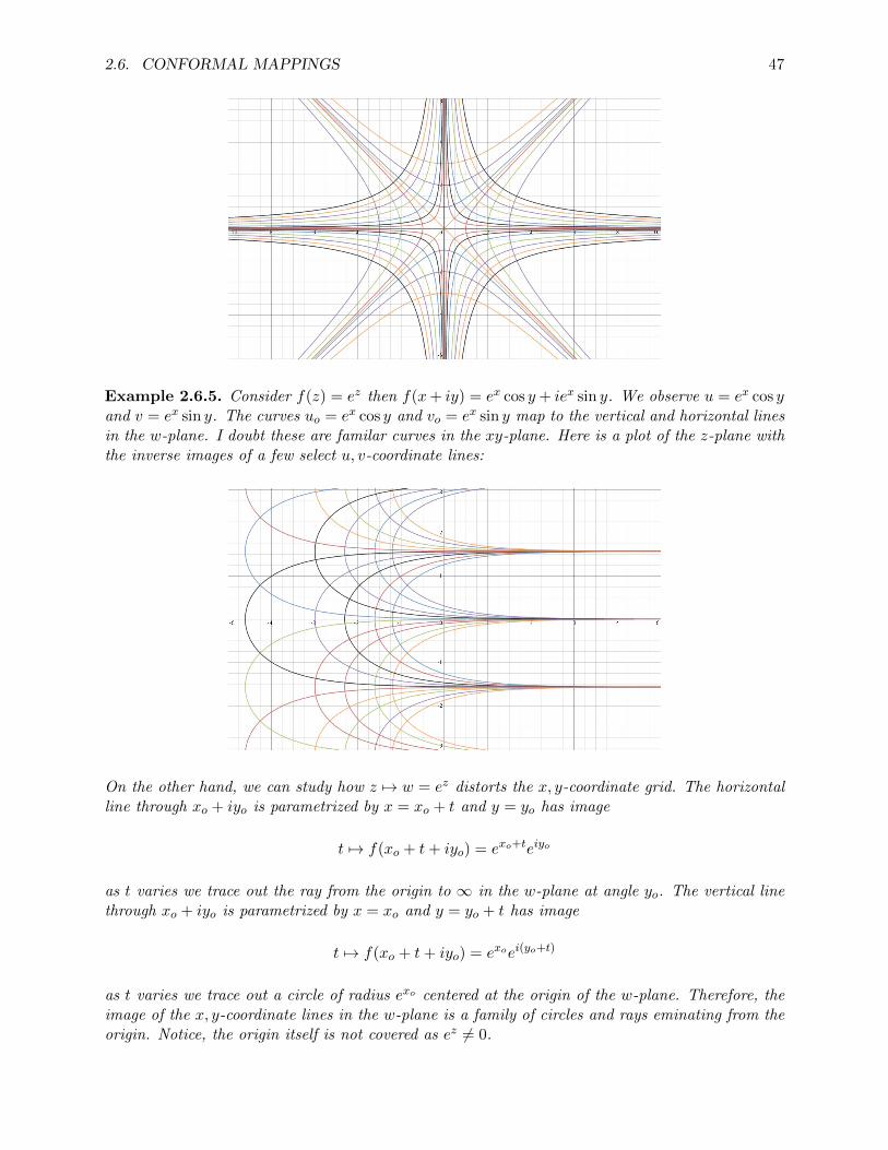
2.6. CONFORMAL MAPPINGS 47
Example 2.6.5. Consider f(z) = ez then f(x+ iy) = ex cos y+ iex sin y. We observe u = ex cos yand v = ex sin y. The curves uo = ex cos y and vo = ex sin y map to the vertical and horizontal linesin the w-plane. I doubt these are familar curves in the xy-plane. Here is a plot of the z-plane withthe inverse images of a few select u, v-coordinate lines:
On the other hand, we can study how z 7→ w = ez distorts the x, y-coordinate grid. The horizontalline through xo + iyo is parametrized by x = xo + t and y = yo has image
t 7→ f(xo + t+ iyo) = exo+teiyo
as t varies we trace out the ray from the origin to ∞ in the w-plane at angle yo. The vertical linethrough xo + iyo is parametrized by x = xo and y = yo + t has image
t 7→ f(xo + t+ iyo) = exoei(yo+t)
as t varies we trace out a circle of radius exo centered at the origin of the w-plane. Therefore, theimage of the x, y-coordinate lines in the w-plane is a family of circles and rays eminating from theorigin. Notice, the origin itself is not covered as ez 6= 0.

48 CHAPTER II. ANALYTIC FUNCTIONS
There is another simple calculation to see the orthogonality of constant u or v curves. Calculate∇u = 〈ux, uy〉 and ∇v = 〈vx, vy〉. But, if f = u + iv is holomorphic then ux = vy and vx = −uy.By CR-equations,
∇u = 〈ux, uy〉 = 〈vy,−vx〉
but, ∇v = 〈vx, vy〉 hence ∇u •∇v = 0. Of course, this is just a special case of our general result onconformality of holomorphic maps.
2.7 Fractional Linear Transformations
Definition 2.7.1. Let a, b, c, d ∈ C such that ad− bc 6= 0. A fractional linear transformation
or Mobius transformation is a function of the form f(z) =az + b
cz + d. If f(z) = az then f is
a dilation. If f(z) = z + b then f is a translation. If f(z) = az + b then f is an affinetransformation. If f(z) = 1/z then f is an inversion.
The quotient rule yields f ′(z) =a(cz + d)− (az + b)c
(cz + d)2=
ad− bc(cz + d)2
thus the condition ad− bc 6= 0
is the requirement that f(z) not be constant. Gamelin shows through direct calculation that iff and g are Mobius transformations then the composite f ◦ g is also a mobius transformation. Itturns out the set of all Mobius transformations forms a group under composition. This group offractional linear transformations is built from affine transformations and inversions. In particular,
consider f(z) =az + b
cz + d. If c = 0 then f(z) = a
dz+ bd which is just an affine transformation. On the
other hand, if c 6= 0 then
f(z) =az + b
cz + d=
ac (cz + d)− ad
c + b
cz + d=a
c+bc− ad
c
1
cz + d
This expression can be seen as the composition of the maps below:
f1(z) =a
c+bc− ad
cz & f2(z) =
1
z& f3(z) = cz + d
In particular, f = f1 ◦ f2 ◦ f3. This provides proof similar to that given in Gamelin page 65:
Theorem 2.7.2. Every fractional linear transformation is the composition of dilations, translationsand inversions.
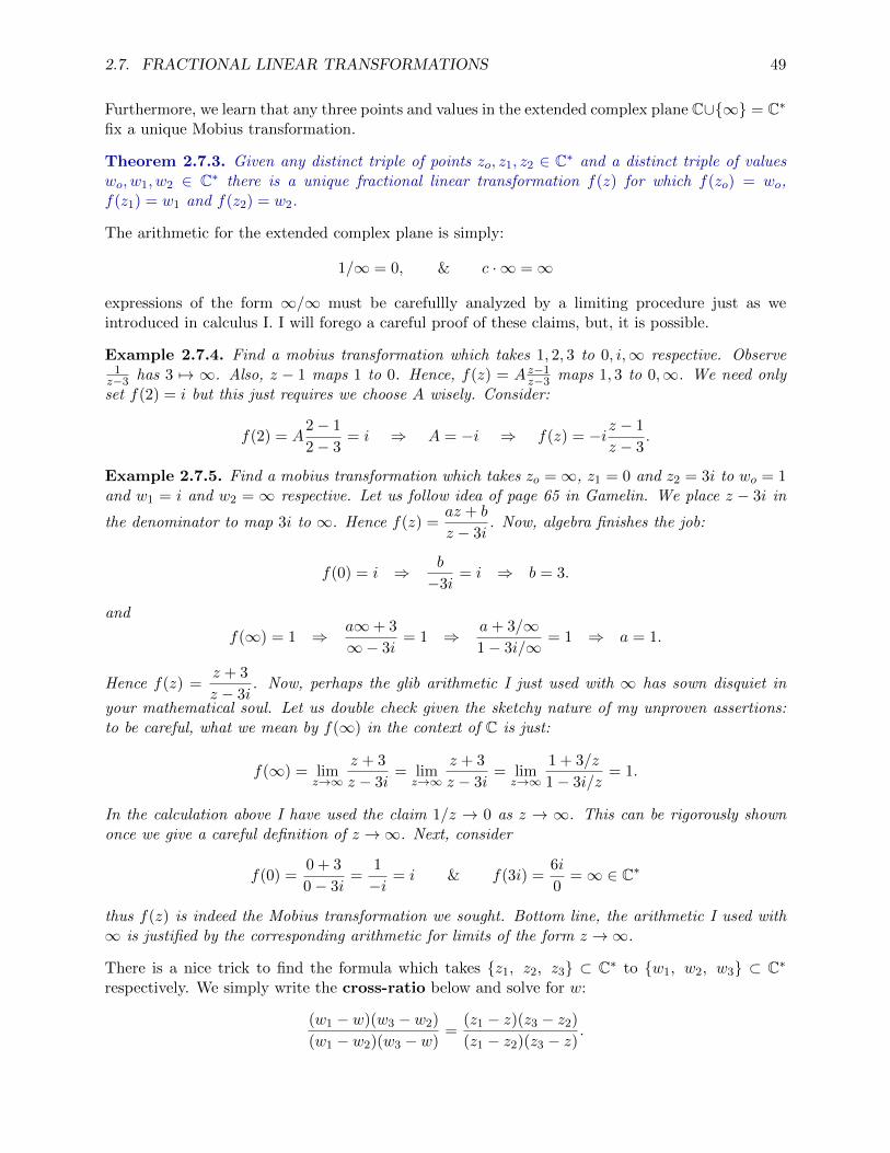
2.7. FRACTIONAL LINEAR TRANSFORMATIONS 49
Furthermore, we learn that any three points and values in the extended complex plane C∪{∞} = C∗fix a unique Mobius transformation.
Theorem 2.7.3. Given any distinct triple of points zo, z1, z2 ∈ C∗ and a distinct triple of valueswo, w1, w2 ∈ C∗ there is a unique fractional linear transformation f(z) for which f(zo) = wo,f(z1) = w1 and f(z2) = w2.
The arithmetic for the extended complex plane is simply:
1/∞ = 0, & c · ∞ =∞
expressions of the form ∞/∞ must be carefullly analyzed by a limiting procedure just as weintroduced in calculus I. I will forego a careful proof of these claims, but, it is possible.
Example 2.7.4. Find a mobius transformation which takes 1, 2, 3 to 0, i,∞ respective. Observe1z−3 has 3 7→ ∞. Also, z − 1 maps 1 to 0. Hence, f(z) = A z−1
z−3 maps 1, 3 to 0,∞. We need onlyset f(2) = i but this just requires we choose A wisely. Consider:
f(2) = A2− 1
2− 3= i ⇒ A = −i ⇒ f(z) = −iz − 1
z − 3.
Example 2.7.5. Find a mobius transformation which takes zo =∞, z1 = 0 and z2 = 3i to wo = 1and w1 = i and w2 = ∞ respective. Let us follow idea of page 65 in Gamelin. We place z − 3i in
the denominator to map 3i to ∞. Hence f(z) =az + b
z − 3i. Now, algebra finishes the job:
f(0) = i ⇒ b
−3i= i ⇒ b = 3.
and
f(∞) = 1 ⇒ a∞+ 3
∞− 3i= 1 ⇒ a+ 3/∞
1− 3i/∞= 1 ⇒ a = 1.
Hence f(z) =z + 3
z − 3i. Now, perhaps the glib arithmetic I just used with ∞ has sown disquiet in
your mathematical soul. Let us double check given the sketchy nature of my unproven assertions:to be careful, what we mean by f(∞) in the context of C is just:
f(∞) = limz→∞
z + 3
z − 3i= lim
z→∞
z + 3
z − 3i= lim
z→∞
1 + 3/z
1− 3i/z= 1.
In the calculation above I have used the claim 1/z → 0 as z → ∞. This can be rigorously shownonce we give a careful definition of z →∞. Next, consider
f(0) =0 + 3
0− 3i=
1
−i= i & f(3i) =
6i
0=∞ ∈ C∗
thus f(z) is indeed the Mobius transformation we sought. Bottom line, the arithmetic I used with∞ is justified by the corresponding arithmetic for limits of the form z →∞.
There is a nice trick to find the formula which takes {z1, z2, z3} ⊂ C∗ to {w1, w2, w3} ⊂ C∗respectively. We simply write the cross-ratio below and solve for w:
(w1 − w)(w3 − w2)
(w1 − w2)(w3 − w)=
(z1 − z)(z3 − z2)
(z1 − z2)(z3 − z).

50 CHAPTER II. ANALYTIC FUNCTIONS
This is found in many complex variables texts. I found it in Complex Variables: Introduction andApplications second ed. by Mark J. Ablowitz and Athanassios S. Fokas; see their §5.7 on bilineartransformations14. I tend to consult Ablowitz and Fokas for additional computational ideas. It’sa bit beyond what I intend for this course computationally.
Example 2.7.6. Let us try out this mysterious cross-ratio. We seek the map of {i,∞, 3} to{∞, 0, 1}. Consider,
(∞− w)(1− 0)
(∞− 0)(1− w)=
(i− z)(3−∞)
(i−∞)(3− z).
This simplifies to:
1
1− w=i− z3− z
⇒ 1− w =3− zi− z
⇒ w = 1− 3− zi− z
=z − 3 + i− z
i− z=i− 3
i− z.
Define f(z) = i−3i−z and observe f(i) =∞, f(∞) = 0 and f(3) = i−3
i−3 = 1.
There are many variations on the examples given above, but, I hope that is enough to get youstarted. Beyond finding a particular Mobius transformation, it is also interesting to study whathappens to various curves for a given Mobius transformation. In particular, the theorem below isbeautifully simple and reason enough for us to discuss C∗ in this course:
Theorem 2.7.7. A fractional linear transformation maps circles to circles in the extended complexplane to circles in the extended complex plane
Recall that a line is a circle through ∞ in the context of C∗. You might think I’m just doing mathfor math’s sake here15, but, there is actually application of the observations of this section to theproblem of conformal mapping. We later learn that conformal mapping allows us to solve Laplace’sequation by transferrring solutions through conformal maps. Therefore, the problem we solve hereis one step towards find the voltage function for somewhat complicated boundary conditions in theplane. Or, solving certain problems with fluid flow. Gamelin soon returns to these applications infuture chapters, I merely make this comment here to give hope to those who miss applications.
Recall, if D is a domain then O(D) the set of holomorphic functions from D to C.
Definition 2.7.8. Let D be a domain, we say f ∈ O(D) is biholomorphic mapping of D ontoD′ if f(D) = D′ and f−1 : D′ → D is holomorphic.
In other words, a biholomorphic mapping is a bijection which is a holomorphic map with holomor-phic inverse map. These sort of maps are important because they essentially describe coordinatechange maps for C, or from another perspective, they give us a way to produce new domains fromold. The fractional linear transformations are important examples of biholomorphic maps on C.However, the restriction of a fractional linear transformation is also worthy of study. In particular,we find below the restriction of a mobius transformation to a half-plane may give us an image whichis a disk.
As is often the case, this construction is due to Cayley. The Cayley Map is simply a particularexample of a linear fractional transformation. In what follows here I share some insights I foundon pages 80-84 of [R91].
14I would not use this term, but, some folks use this as yet another label for Mobius transformation or frac-tional linear transformation. You might wonder why this cross-ratio technique provides the desired fractional lineartransformation. I welcome you to explain it to me in office hours.
15which is, incidentally, totally fine

2.7. FRACTIONAL LINEAR TRANSFORMATIONS 51
Example 2.7.9. Let h(z) = z−iz+i be defined for z ∈ H where H = {z ∈ C | Im(z) > 0} is the open
upper half-plane. It can be shown that h(z) ∈ E where E = {z ∈ C | |z| ≤ 1} is the closed unitdisk. To see how you might derive this function simply imagine mapping {0, 1,∞} of the boundaryof H to the points {−1,−i, 1}. Fun fact, if you walk along the boundary of a subset of the planethen the interior of the set is on your left if you are wolking in the positively oriented sense. Itis also known that a holomorphic map preserves orientations which implies that boundaries mapto boundaries and points which were locally left of the boundary get mapped to points which arelocally left of the image curve. In particular, note {0, 1,∞} on the boundary of H in the domainmap to the points {−1,−i, 1} on the unit-circle under the mobius transformations. Furthermore,we see the unit-circle given a CCW orientation. The direction of the curve is implicit within thefact that the triple {0, 1,∞} is in the order in which they are found on ∂H so likewise {−1,−i, 1}are in order (this forces CCW orientiation of the image circle). Perhaps a picture is helpful:
I skipped the derivation of h(z) in the example above. We could use the cross-ratio or the techniquesdiscussed earlier. The larger point made by Remmert here is that this transformation is naturalto seek out and in some sense explains why we’ve been studying fractional linear transformationsfor 200+ years. Actually, I’m not sure the precise history of these. I think it is fair to conjectureMobius, Cauchy and Gauss were involved. But, as with any historical conjecture of this period,it seems wise to offer Euler as a possibility, surely he at least looked at these from a real variableviewpoint.
The next thing you might try is to square h−1 of the mapping above. If we feed z 7→ z2 the
open half-plane then the image will be a slit-complex plane. In total z 7→(z+1z−1
)2: E → C− is
a surjection indeed we can even verify this is a biholomorphic mapping. It turns out the slit isa necessary feature, no amount of tinkering can remove it and obtain all of C while maintainingthe biholomorphicity of the map. In fact, Liouville’s Theorem forbids a biholomorphic mapping ofthe disk onto C. But, Riemann in 185116 showed that every simply connected proper subset of Ccan be biholomorphically mapped onto the unit-disk. In this section, we have simply exposed themachinery to make that happen for simple sets like half-planes. A vast literature exists for morecomplicated domains.
16Riemann’s study of complex analysis was centered around the study of conformal mappings, this result is knownas ”Riemann Mapping Theorem” see apge 295 of Gamelin for further discussion.

52 CHAPTER II. ANALYTIC FUNCTIONS

Chapter III
Line Integrals and HarmonicFunctions
In this chapter we review and generalize some basic constructions in multivariate calculus. Gen-eralize in the sense that we analyze complex-valued vector fields over C. We remind the readerhow Green’s Theorem connects to both Stokes’ and Gauss’ Theorems as the line integral allowsus to calculate both circulation and flux in two-dimensions. We analyze the interplay betweenpath-independence, vanishing loop integrals, exact and closed differential forms. Complex analysisenters mainly in our discussion of harmonic conjugates. When u+ iv is holomorphic this indicatesu, v are both solutions of Laplace’s equation and they have orthogonal level curves. This simpleobservation motivates us to use complex analysis to solve Laplace’s equation in the plane. In par-ticular, we examine how fluid flow problems may be solved by selecting an appropriate holomorphicfunction on a given domain. Heat and electrostatics are also briefly discussed.
3.1 Line Integrals and Green’s Theorem
The terminology which follows here is not universally used. As you read different books the termscurve and path are sometimes overloaded with particular technical meanings. In my view, this isthe case with the term ”curve” as defined below.
Definition 3.1.1. A path γ : I ⊆ R→ C is a continuous function. We usually either have I = [a, b]or I = R. If γ is a path such that γ(s) 6= γ(t) for s 6= t then γ is simple. If the path begins andends at the same point then γ is said to be closed. A simple closed path is of the form γ : [a, b]→ Csuch that γ(s) 6= γ(t) for all s 6= t with a ≤ s, t < b and γ(a) = γ(b). The component functionsof γ = x + iy are x and y respective. We say γ is smooth if it has smooth component functions.A continuous path which is built by casewise-joining of finitely many smooth paths is a piecewisesmooth path or simply a curve.
53

54 CHAPTER III. LINE INTEGRALS AND HARMONIC FUNCTIONS
In other texts, the term curve is replaced with arc or contour. In this course I follow Gamelin’sterminology1.
Definition 3.1.2. A path γ : I ⊆ R→ C has trace γ(I).
The trace of a path is the pointset in C which the path covers.
Definition 3.1.3. A path γ : [a, b] → C has reparametrization γ if there is a smooth injectivefunction h : [a, b]→ [a, b] such that γ(t) = γ(h(t)). If h is strictly increasing then γ shares the samedirection as γ. If h is strictly decreasing then γ has direction opposite to that of γ.
The direction of a curve is important since the line-integral is sensitive to the orientation of curves.Furthermore, to be careful, whenever a geometric definition is given we ought to show the defini-tion is independent of the choice of parametrization for the curve involved. The technical detailsof such soul-searching amounts to taking an arbtrary reparametrization (or perhaps all orientationpreserving reparametrizations) and demonstrating the definition naturally transforms.
Definition 3.1.4. Let P be complex values and continuous near the trace of γ : [a, b]→ C. Define:∫γP dx =
∫ b
aP (γ(t))
dRe(γ)
dtdt &
∫γP dy =
∫ b
aP (γ(t))
dIm(γ)
dtdt.
If we use the usual notation γ = x+ iy then the definitions above look like a u-substitution:∫γP dx =
∫ b
aP (x(t), y(t))
dx
dtdt &
∫γP dy =
∫ b
aP (x(t), y(t))
dy
dtdt
These integrals have nice linearity properties.
Theorem 3.1.5. For f, g continuous near the trace of γ and c ∈ C:∫γ(f + cg)dx =
∫γf dx+ c
∫γg dx &
∫γ(f + cg)dy =
∫γf dy + c
∫γg dy.
We define sums of the integrals over dx and dy in the natural manner:∫γP dx+Qdy =
∫γP dx+
∫γQdy.
At first glance this seems like it is merely calculus III restated. However, you should notice thatP and Q are complex-valued functions. That said, if both P,Q are real then ~F = 〈P,Q〉 is areal-vector field in the plane and the standard line-integral from multivariate calculus is precisely:∫
γ
~F • d~r =
∫γP dx+Qdy.
1in other courses, my default is to call the parametrization of a curve a path. For me, a curve is the point-setwhereas a path is a mapping from R into whatever space is considered. Gamelin uses the term ”trace” in the placeof my usual term ”curve”

3.1. LINE INTEGRALS AND GREEN’S THEOREM 55
You should recall the integral above calculates the work done by ~F along the path γ. Continuing,suppose we drop the condition that P,Q be real. Instead, consider P = P1 + iP2 and Q = Q1 + iQ2.Consider: ∫
γP dx+Qdy =
∫γ(P1 + iP2) dx+ (Q1 + iQ2) dy
=
∫γP1 dx+ i
∫γP2 dx+
∫γQ1 dy + i
∫γQ2 dy
=
(∫γP1 dx+
∫γQ1 dy
)+ i
(∫γP2 dx+
∫γQ2 dy
)=
∫γ〈P1, Q1〉 • d~r + i
∫γ〈P2, Q2〉 • d~r.
Therefore, we can interpret the∫γ P dx + Qdy as the complex sum of the work done by the
force 〈Re(P ),Re(Q)〉 and i times the work done by 〈Im(P ), Im(Q)〉 along γ. Furthermore, as theunderlying real integrals are invariant under an orientation preserving reparametrization γ of γ itfollows
∫γ Pdx + Qdy =
∫γ Pdx + Qdy. In truth, these integrals are not the objects of primary
interest in complex analysis. We merely discuss them here to gain the computational basis for thecomplex integral which is defined by
∫γ fdz =
∫γ fdx+ i
∫γ fdy. We study the complex integral
in Chapter 4.
Example 3.1.6. Let γ1(t) = cos t+ i sin t for 0 ≤ t ≤ π. Then x = cos t and dx = − sin tdt whereasy = sin t and dy = cos tdt. Let P (x+ iy) = y + ix2 and calculate
∫γ1P dx:∫
γ1
(y + ix2) dx =
∫ π
0
(sin t+ i cos2 t
)(− sin tdt)
= −∫ π
0sin2 t− i
∫ π
0cos2 t sin tdt
= −π2
+ iu3
3
∣∣∣∣−1
1
= −π2− i2
3.
To integrate along a curve we simply sum the integrals along the smooth paths which join to formthe curve. In particular:
Definition 3.1.7. Let γ be a curve formed by joining the smooth paths γ1, γ2, . . . , γn. In terms ofthe trace denoted trace(γ) = [γ] we have [γ] = [γ1]∪ [γ2]∪ · · · ∪ [γn] Let P,Q be complex valued andcontinuous near the trace of γ. Define:∫
γP dx+Qdy =
n∑j=1
∫γj
P dx+Qdy.
I assume the reader can define∫γ P dx and
∫γ Qdy for a curve in the same fashion. Let us continue
Example 3.1.6.
Example 3.1.8. Let γ2(t) = −1 + 2t for 0 ≤ t ≤ 1. This is the natural parametrization of theline-segment [−1, 1]. Let γ1 be as in Example 3.1.6 and define γ = γ1 ∪ γ2. We seek to calculate

56 CHAPTER III. LINE INTEGRALS AND HARMONIC FUNCTIONS
∫γ P dx where P (x + iy) = y + ix2. Let us consider γ2, in this path we have x = −1 + 2t hence
dx = 2dt whereas y = 0 so dy = (0)dt. Thus,∫γ2
(y + ix2)dx =
∫ 1
0
(0 + i(−1 + 2t)2
)(2dt) = 2i
∫ 1
0
(1− 4t+ 4t2
)= 2i
(1− 4
2+
4
3
)=
2i
3.
Thus, ∫γP dx =
∫γ1
P dx+
∫γ2
P dx = −π2− i2
3+
2i
3= −π
2.
In order to state the complex-valued version of Green’s Theorem we define complex-valued areaintegrals and partial derivatives of complex-valued functions2:
Definition 3.1.9. Let F and G be real-valued functions on C = R2 then we define:∫∫S
(F + iG)dA =
∫∫SF dA+ i
∫∫SGdA.
∂
∂x
(F + iG
)=∂F
∂x+ i
∂G
∂x
The double integral∫∫S f dA =
∫∫S f(x, y)dx dy and partial derivatives above are discussed in detail
in multivariable calculus. We calculate these integrals by iterated integrals over type I or II regionsor polar coordinate substitution.
Theorem 3.1.10. Complex-valued Green’s Theorem: Let γ be a simple closed curve which formsthe boundary of S in the positively oriented sense; that is, S ⊆ C and ∂S = γ:∫
γP dx+Qdy =
∫∫S
(∂Q
∂x− ∂P
∂y
)dA.
Proof: let P = P1 + iP2 and Q = Q1 + iQ2 where P1, P2, Q1, Q2 are all real-valued functions.Observe, from our discussion ealier in this section,∫
γP dx+Qdy =
(∫γP1 dx+
∫γQ1 dy
)+ i
(∫γP2 dx+
∫γQ2 dy
)however, we also have:∫∫
S
(∂Q
∂x− ∂P
∂y
)dA =
∫∫S
(∂Q1
∂x− ∂P1
∂y
)dA+ i
∫∫S
(∂Q2
∂x− ∂P2
∂y
)dA.
Finally, by Green’s Theorem for real-valued double integrals we obtain:∫γPj dx+
∫γQj dy =
∫∫S
(∂Qj∂x− ∂Pj
∂y
)dA.
for j = 1 and j = 2. Therefore,
∫γP dx+Qdy =
∫∫S
(∂Q
∂x− ∂P
∂y
)dA. �
Of course, I have taken a rather different path from that in Gamelin. He gives a proof of Green’sTheorem based on deriving Green’s Theorem for a triangle, stretching the theorem to a curvedtriangle then summing over a triangulazation of the space. It is a nice, standard, argument. Imight go over it in lecture. See pages 357-367 of my 2014 Multivariable Calculus notes for a proofof Green’s Theorem based on a rectangularization of a space. I will not replicate it here.
2we have used this idea before. For example, when I wrote dfdz
= ∂f∂x
= ux + ivx.

3.1. LINE INTEGRALS AND GREEN’S THEOREM 57
Example 3.1.11. We now attack Example 3.1.8 with the power of Green’s Theorem. ConsiderP = y+ ix2 and Q = 0. Apply Green’s Theorem with Q = 0 we have (remember S is the upper-halfof the unit-disk) ∫
γP dx = −
∫∫S
∂P
∂ydA = −
∫∫SdA = −π
2.
Very well, we have almost good agreement between Example 3.1.11 and Example 3.1.8. I now amsure there is an error in what is currently written. First person to find the error and email me thecorrection in detail earns 5pts bonus.
A comment from the future: In view of the results of the next section there is a natural reasonwhy P = y+ ix2 has different behaviour for P1 = y and P2 = x2. In particular, the differential ydxis not an exact form on the half-disk whereas x2dx = d(x3/3) hence x2dx is exact.
In order to calculate integrals in the complex plane we need to be able to parametrize the paths ofinterest. In particular, you should be ready, willing, and able to parametrize lines, circles and allmanner of combinations thereof. The next example illustrates how two dimensional vector problemsare nicely simplified by the use of complex notation.
Example 3.1.12. Let γ be the curve formed by the rays γ1, γ3 at θ = π/6 and θ = π/3 and thearcs γ4, γ1 connecting the rays along |z| = 1 and |z| = 2. Assume γ is positively oriented and thepicture below helps explain my choice of numbering:
In detail: the rays are parametrized by γ1(t) = teiπ/6 = t(√
3 + i)/2 for 1 ≤ t ≤ 2 and γ3(t) =−teiπ/3 = −t(1 + i
√3)/2 for −2 ≤ t ≤ −1. The arcs are given by γ2(t) = 2eit for π/6 ≤ t ≤ π/3
and γ4(t) = e−it for −π/3 ≤ t ≤ −π/6. If we let γ−4 denote the reverse of γ4 then we have thenatural parametrization γ−4(t) = eit for π/6 ≤ t ≤ π/3. In practice, it’s probably better to use thereversed curve and simply place a minus in to account for the reversed path. I use this idea in whatfollows. Consider then, for γ1 we have x = t
√3/2 and y = t/2 hence dy = dt/2 and:∫
γ1
x dy =
∫ 2
1(t√
3/2)(dt/2) =
√3
4
t2
2
∣∣∣∣21
=
√3
4
[4
2− 1
2
]=
3√
3
8.
For γ2 observe x = 2 cos t whereas y = 2 sin t hence dy = 2 cos t dt and:∫γ2
x dy =
∫ π/3
π/6(2 cos t)(2 cos tdt)
=
∫ π/3
π/64 cos2 tdt
= 2
∫ π/3
π/6[1 + cos(2t)]dt = 2
(π
3− π
6+
1
2sin
(2π
3
)− 1
2sin
(2π
6
))=π
3.

58 CHAPTER III. LINE INTEGRALS AND HARMONIC FUNCTIONS
Next, consider γ−3(t) = t(1 + i√
3)/2 for 1 ≤ t ≤ 2. This is the reversal of γ3. We have x = t/2and y = t
√3/2 hence dy =
√3dt/2 hence:∫
γ−3
x dy =
∫ 2
1(t/2)(
√3dt/2) =
√3
4
t2
2
∣∣∣∣21
=
√3
4
[4
2− 1
2
]=
3√
3
8.
Last, γ4 has reversal γ−4(t) = eit = cos t+ i sin t thus x = cos t and dy = cos tdt∫γ−4
x dy =
∫ π/3
π/6(cos t)(cos tdt)
=
∫ π/3
π/6cos2 tdt
=1
2
∫ π/3
π/6[1 + cos(2t)]dt =
1
2
(π
3− π
6+
1
2sin
(2π
3
)− 1
2sin
(2π
6
))=
π
12.
In total, we have:∫γx dy =
∫γ1
x dy +
∫γ2
x dy −∫γ−3
x dy −∫γ−4
x dy =3√
3
8+π
3− 3√
3
8− π
12=
π
4.
Let us check our work by using Green’s Theorem on Q = x and P = 0. Let S be as in the diagramhence γ = ∂S is the positively oriented boundary for which Green’s Theorem applies:
∫γx dy =
∫∫SdA =
∫ π/3
π/6
∫ 2
1r dr dθ =
(∫ π/3
π/6dθ
)(∫ 2
1r dr
)=[π
3− π
6
] [22
2− 12
2
]=
3π
12=π
4.
I think it is fairly clear from this example that we should use Green’s Theorem when possible.
3.2 Independence of Path
The theorems we cover in this section should all be familar from your study of multivariate calculus.That said, we do introduce some new constructions allowing for complex-valued components. I’llsay more about the correspondence between what we do here and the usual multivariate calculusat the conclusion of this section.
The total differential of a complex function u+ iv is defined by du+ idv where du and dv are theusual total differentials from multivariate calculus. This is equivalent to the definition below:
Definition 3.2.1. If h is a complex-valued function which has continuous real partial derivativefunctions hx, hy then the differential dh of h is
dh =∂h
∂xdx+
∂h
∂ydy.
A differential form Pdx+Qdy is said to be exact on U ⊆ C if there exists a function h for whichdh = Pdx+Qdy for each point in U .

3.2. INDEPENDENCE OF PATH 59
Recall from calculus I, if F ′(t) = f(t) for all t ∈ [a, b] then the FTC states∫ ba f(t)dt = F (b)−F (a).
If we write this in a slightly different notation then the analogy to what follows is even more clear.In particular F ′ = dF/dt so F ′(t) = f(t) means dF = f(t) dt hence by an F -substitution,∫ b
af(t)dt =
∫ F (b)
F (a)dF = F (b)− F (a).
You can see that f(t)dt is to F as Pdx+Qdy is to h.
Theorem 3.2.2. If γ is a piecewise smooth curve from A to B and h is continuously (real) differ-
entiable near γ with dh = Pdx+Qdy then
∫γPdx+Qdy =
∫γdh = h(B)− h(A).
Proof: the only thing we need to show is∫γ dh = h(B) − h(A). The key point is that if γ(t) =
x(t) + iy(t) then by the chain-rule:
d
dth(γ(t)) =
d
dth(x(t), y(t)) =
∂h
∂x
dx
dt+∂h
∂y
dy
dt.
We assume γ : [a, b]→ C has γ(a) = A and γ(b) = B. Thus,∫γdh =
∫γ
∂h
∂xdx+
∂h
∂ydy =
∫ b
a
(∂h
∂x
dx
dt+∂h
∂y
dy
dt
)dt
=
∫ b
a
d
dt
(h(γ(t))
)dt
= h(γ(b))− h(γ(a))
= h(B)− h(A). �
When we integrate∫γ Pdx + Qdy for an exact differential form Pdx + Qdy = dh then there is
no need to work out the details of the integration. Thankfully we can simply evaluate h at theend-points.
Example 3.2.3. Let γ be some path from i to 1 + i.∫γ(y + 3x2)dx+ (x+ 4y3)dy =
∫ 1+2i
id(xy + x3 + y4
)=(1(2i) + 13 + (2i)4
)− i4
= 2i+ 1 + 16− 1
= 16 + 2i.
The replacement of the notation∫γ with
∫ 1+2ii is only reasonable if the integral dependends only on
the endpoints. Theorem 3.2.2 shows this is true whenever Pdx+Qdy is exact near the integration.
To make it official, let me state the definition clearly:
Definition 3.2.4. The differential form Pdx + Qdy is independent of path in U ⊆ C if forevery pair of curves γ1, γ2 in U with matching starting and ending points have
∫γ1Pdx + Qdy =∫
γ2Pdx+Qdy.
An equivalent condition to independence of path is given by the vanishing of all integrals aroundloops; a loop is just a simple closed curve.
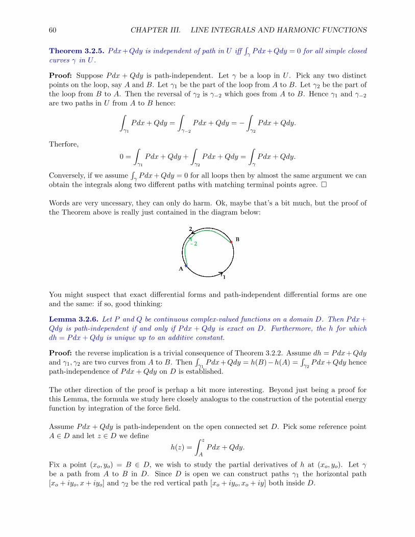
60 CHAPTER III. LINE INTEGRALS AND HARMONIC FUNCTIONS
Theorem 3.2.5. Pdx+Qdy is independent of path in U iff∫γ Pdx+Qdy = 0 for all simple closed
curves γ in U .
Proof: Suppose Pdx + Qdy is path-independent. Let γ be a loop in U . Pick any two distinctpoints on the loop, say A and B. Let γ1 be the part of the loop from A to B. Let γ2 be the part ofthe loop from B to A. Then the reversal of γ2 is γ−2 which goes from A to B. Hence γ1 and γ−2
are two paths in U from A to B hence:∫γ1
Pdx+Qdy =
∫γ−2
Pdx+Qdy = −∫γ2
Pdx+Qdy.
Therfore,
0 =
∫γ1
Pdx+Qdy +
∫γ2
Pdx+Qdy =
∫γPdx+Qdy.
Conversely, if we assume∫γ Pdx+Qdy = 0 for all loops then by almost the same argument we can
obtain the integrals along two different paths with matching terminal points agree. �
Words are very uncessary, they can only do harm. Ok, maybe that’s a bit much, but the proof ofthe Theorem above is really just contained in the diagram below:
You might suspect that exact differential forms and path-independent differential forms are oneand the same: if so, good thinking:
Lemma 3.2.6. Let P and Q be continuous complex-valued functions on a domain D. Then Pdx+Qdy is path-independent if and only if Pdx + Qdy is exact on D. Furthermore, the h for whichdh = Pdx+Qdy is unique up to an additive constant.
Proof: the reverse implication is a trivial consequence of Theorem 3.2.2. Assume dh = Pdx+Qdyand γ1, γ2 are two curves from A to B. Then
∫γ1Pdx+Qdy = h(B)−h(A) =
∫γ2Pdx+Qdy hence
path-independence of Pdx+Qdy on D is established.
The other direction of the proof is perhap a bit more interesting. Beyond just being a proof forthis Lemma, the formula we study here closely analogus to the construction of the potential energyfunction by integration of the force field.
Assume Pdx + Qdy is path-independent on the open connected set D. Pick some reference pointA ∈ D and let z ∈ D we define
h(z) =
∫ z
APdx+Qdy.
Fix a point (xo, yo) = B ∈ D, we wish to study the partial derivatives of h at (xo, yo). Let γbe a path from A to B in D. Since D is open we can construct paths γ1 the horizontal path[xo + iyo, x+ iyo] and γ2 be the red vertical path [xo + iyo, xo + iy] both inside D.

3.2. INDEPENDENCE OF PATH 61
Notice the point at the end of γ1 is x+ iyo and:
h(x+ iyo) =
∫γPdx+Qdy +
∫γ1
Pdx+Qdy
However, γ1 has x = t for xo ≤ t ≤ x and y = yo hence dx = dt and dy = 0,
h(x+ iyo) =
∫γPdx+Qdy +
∫ x
xo
P (t, yo)dt.
Notice γ has no dependence on x thus:
∂
∂xh(x+ iyo) =
∂
∂x
∫ x
xo
P (t, yo)dt = P (x, yo).
where we have used the FTC in the last equality. Next, note γ1 ends at xo + iy thus:
h(xo + iy) =
∫γPdx+Qdy +
∫γ2
Pdx+Qdy
But, γ2 has x = xo and y = t for yo ≤ t ≤ y thus dx = 0 and dy = dt. We find
h(xo + iy) =
∫γPdx+Qdy +
∫ y
yo
Q(xo, t)dt
Notice γ has no dependence on y thus:
∂
∂yh(xo + iy) =
∂
∂y
∫ y
yo
Q(xo, t)dt = Q(xo, y).
In total we have shown hx(x, yo) = P (x, yo) and hy(xo, y) = Q(xo, y). By continuity of P and Qwe find dh = Pdx + Qdy at (xo, yo). However, (xo, yo) is an arbitrary point of D and it followsPdx+Qdy is exact on D with potential h(z) =
∫ zA Pdx+Qdy.
Finally, to study uniqueness, suppose h1 is another function on D for which dh1 = Pdx + Qdy.Notice dh = dh1 thus d(h − h1) = 0 but this implies ∇Re(h − h1) = 0 and ∇Im(h − h1) = 0thus both the real and imaginary components of h− h1 are constant and we find h = h1 + c. Thefunction h is uniquely associated to Pdx+Qdy on a domain up to an additive constant. �
I usually say that h is the potential for Pdx+Qdy modulo an additive constant. If all differentialforms were exact then integration would be much easier and life would not be so interesting.Fortunately, only some forms are exact. The following definition is a natural criteria to investigatesince P = ∂h
∂x and Q = ∂h∂y suggest that P and Q are related by differentiation due to Clairaut’s
theorem on commuting partial derivatives. We expect ∂∂y
∂h∂x = ∂
∂x∂h∂y hence ∂P
∂y = ∂Q∂x . Thus define:
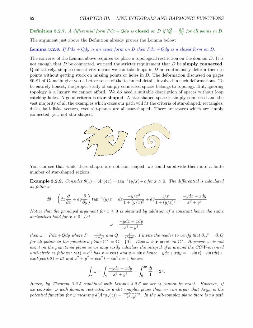
62 CHAPTER III. LINE INTEGRALS AND HARMONIC FUNCTIONS
Definition 3.2.7. A differential form Pdx+Qdy is closed on D if ∂Q∂x = ∂P
∂y for all points in D.
The argument just above the Definition already proves the Lemma below:
Lemma 3.2.8. If Pdx+Qdy is an exact form on D then Pdx+Qdy is a closed form on D.
The converse of the Lemma above requires we place a topological restriction on the domain D. It isnot enough that D be connected, we need the stricter requirement that D be simply connected.Qualitatively, simple connectivity means we can take loops in D an continuously deform them topoints without getting stuck on missing points or holes in D. The deformation discussed on pages80-81 of Gamelin give you a better sense of the technical details involved in such deformations. Tobe entirely honest, the proper study of simply connected spaces belongs to topology. But, ignoringtopology is a luxury we cannot afford. We do need a suitable description of spaces without loopcatching holes. A good criteria is star-shaped. A star-shaped space is simply connected and thevast majority of all the examples which cross our path will fit the criteria of star-shaped; rectangles,disks, half-disks, sectors, even slit-planes are all star-shaped. There are spaces which are simplyconnected, yet, not star-shaped:
You can see that while these shapes are not star-shaped, we could subdivide them into a finitenumber of star-shaped regions.
Example 3.2.9. Consider θ(z) = Arg(z) = tan−1(y/x)+c for x > 0. The differential is calculatedas follows:
dθ =
(dx
∂
∂x+ dy
∂
∂y
)tan−1(y/x = dx
−y/x2
1 + (y/x)2+ dy
1/x
1 + (y/x)2=−ydx+ xdy
x2 + y2
Notice that the principal argument for x ≤ 0 is obtained by addition of a constant hence the samederivatives hold for x < 0. Let
ω =−ydx+ xdy
x2 + y2
then ω = Pdx+Qdy where P = −yx2+y2
and Q = xx2+y2
. I invite the reader to verify that ∂yP = ∂xQ
for all points in the punctured plane C× = C − {0}. Thus ω is closed on C×. However, ω is notexact on the punctured plane as we may easily calculate the integral of ω around the CCW-orientedunit-circle as follows: γ(t) = eit has x = cos t and y = sin t hence −ydx+xdy = − sin t(− sin tdt) +cos t(cos tdt) = dt and x2 + y2 = cos2 t+ sin2 t = 1 hence:∫
γω =
∫γ
−ydx+ xdy
x2 + y2=
∫ 2π
0
dt
1= 2π.
Hence, by Theorem 3.2.5 combined with Lemma 3.2.6 we see ω cannot be exact. However, ifwe consider ω with domain restricted to a slit-complex plane then we can argue that Argα is thepotential function for ω meaning d(Argα(z)) = −ydx+xdy
x2+y2. In the slit-complex plane there is no path

3.2. INDEPENDENCE OF PATH 63
which encircles the origin and the nontrivial loop integral is removed. If we use 1 as a referencepoint for the potential construction then we find the following natural integral presentation of theprincipal argument:
Arg(z) =
∫ z
1
−ydx+ xdy
x2 + y2
The example above is the quintessential example of a form which is closed but not exact. Poincare’sLemma solves this puzzle in more generality. In advanced calculus, I usually share a calculationwhich shows that in any contractible subset of Rn every closed differential p-form is the exteriorderivative of a potential (p− 1)-form. What we study here is almost the most basic case3. Whatfollows is a weakened converse of Lemma 3.2.8; we find if a form is closed on a star-shaped domainthen the form must be exact.
Theorem 3.2.10. If domain D is star-shaped. Then Pdx+Qdy closed in D implies there existsfunction h on D for which dh = Pdx+Qdy in D.
Proof: assume D is a star-shaped domain and Pdx+Qdy is a closed form on D. This means weassume ∂xQ = ∂yP on D. Let A be a star-center for D and define h(z) =
∫[A,z] Pdx+Qdy
Fix a point zo in D and note [A, zo] is in D. Furthermore, γ1 is given by x = t for xo ≤ t ≤ xand y = yo. Likewise, γ2 is the line-segment [zo, xo + iy] where x = xo and y = t for yo ≤ t ≤ y.Note [A, xo + iy] and [A, x+ iyo] are in D. Apply Green’s Theore on the triangle T2 with verticesA, zo, xo + iy: ∫
∂T2
Pdx+Qdy =
∫∫T2
(∂Q
∂x− ∂P
∂y
)dA =
∫∫T2
(0)dA = 0.
3in one-dimension all smooth forms fdx are both closed and exact

64 CHAPTER III. LINE INTEGRALS AND HARMONIC FUNCTIONS
Thus, ∫[A,zo]
Pdx+Qdy +
∫[zo,xo+iy]
Pdx+Qdy +
∫[xo+iy,A]
Pdx+Qdy = 0
but, we defined h(z) =∫
[A,z] Pdx+Qdy thus
h(xo, yo)− h(xo, y) +
∫ y
yo
Q(xo, t)dt = 0 ⇒ ∂h
∂y= Q(xo, y).
Examine triangle T1 formed by A, zo, x + iyo to derive by a very similar argument ∂h∂x = P (x, yo).
Thus, dh = Pdx+Qdy at zo and it follows h(z) =∫
[A,z] Pdx+Qdy serves to define a potential forPdx+Qdy on D. Thus Pdx+Qdy is exact on D. �
Given that we have shown the closed form Pdx+Qdy on star-shaped domain is exact we have byLemma 3.2.6 that Pdx+Qdy is path-independent. It follows we can calculate h(z) along any pathin D, not just [A, z] which was our starting point for the proof above.
The remainder of Gamelin’s section 3.2 is devoted to discussing deformation theorems for closedforms. I give a simplified proof of the deformation. Actually, at the moment, I’m not certain ifGamelin’s proof is more or less general than the one I offer below. There may be a pedagogicalreason for his development I don’t yet appreciate4.
Suppose γup and γdown are two curves from A to B. For simplicity of exposition, let us supposethese curves only intersect at their endpoints. Suppose Pdx + Qdy is a closed form on the regionbetween the curves. We may inquire, does
∫γup
Pdx + Qdy =∫γdown
Pdx + Qdy ? To understand
the resolution of this question we should consider the picture below:
Here I denote γup = γ1 ∪ γ2 and γdown = γ3 ∪ γ4 . The middle points M,N are joined by thecross-cuts γ5 and γ6 = γ−5. Notice that ∂S = γ5 ∪ γ−1 ∪ γ3 whereas ∂T = γ6 ∪ γ4 ∪ γ−2. Now,apply Green’s Theorem to the given closed form on S and T to obtain:∫
∂SPdx+Qdy =
∫∫S
(∂Q
∂x− ∂P
∂y
)dA = 0 &
∫∂TPdx+Qdy =
∫∫T
(∂Q
∂x− ∂P
∂y
)dA = 0.
The double integrals above are zero because we know ∂Q∂x = ∂P
∂y . To complete the argument webreak the line-integrals around the boundary into pieces taking into account the sign-rule for curve
4I think the rolling wave argument is essentially the same as I give here, but I should compare Gamelin’s proof tomine when time permits

3.2. INDEPENDENCE OF PATH 65
reversals: for ∂S = γ5 ∪ γ−1 ∪ γ3 we obtain:∫γ5
Pdx+Qdy −∫γ1
Pdx+Qdy +
∫γ3
Pdx+Qdy = 0
for ∂T = γ6 ∪ γ4 ∪ γ−2 we obtain:∫γ6
Pdx+Qdy +
∫γ4
Pdx+Qdy −∫γ2
Pdx+Qdy = 0.
Summing the two equations above and noting that∫γ6Pdx+Qdy+
∫γ5Pdx+Qdy = 0 we obtain:
(using Gamelin’s slick notation)[−∫γ1
+
∫γ3
+
∫γ4
−∫γ2
](Pdx+Qdy) = 0 ⇒
[∫γ1
+
∫γ2
](Pdx+Qdy) =
[∫γ3
+
∫γ4
](Pdx+Qdy).
Consequently, as γup = γ1 ∪ γ2 and γdown = γ3 ∪ γ4 we conclude∫γup
Pdx+Qdy =
∫γdown
Pdx+Qdy.
We have shown that the integral of a differential form Pdx + Qdy is unchanged if we deform thecurve of integration over a region on which the form Pdx+Qdy is closed5
The construction of the previous page is easily extended to deformations over regions which are notsimply connected. For example, we can argue that if Pdx+Qdy is closed on the crooked annulusthen the integral of Pdx+Qdy on the inner and outer boundaries must conicide.
The argument again centers on the application of Green’s Theorem to simply connected domainson which the area integral vanishes hence leaving the integral around the boundary trivial. Whenwe add the integral around ∂T and ∂S the red cross-cuts vanish. Define γout = γ3 ∪ γ4 andγin = γ−1 ∪ γ−2 (used the reversals to make the curve have a postive orientation). In view of thesedefitions, we find: ∫
γout
Pdx+Qdy =
∫γin
Pdx+Qdy.
The deformation of the inner annulus boundary to the outer boundary leaves the integral unchangedbecause the differential form Pdx+Qdy was closed on the intermediate curves of the deformation.
5 in the langauge of exterior calculus; d(Pdx+Qdy) = (Qx − Py)dx ∧ dy = 0.

66 CHAPTER III. LINE INTEGRALS AND HARMONIC FUNCTIONS
Example 3.2.11. In Example 3.2.9 we learned that the form −ydx+xdyx2+y2
is closed on the punctured
plane C×. We also showed that∫γ−ydx+xdyx2+y2
= 2π where γ is the CCW-oriented unit-circle. Let Cbe any positively oriented loop which encircles the origin we may deform the unit-circle to the loopthrough a region on which the form is closed hence
∫C−ydx+xdyx2+y2
= 2π.
There are additional modifications of Green’s Theorem for regions with finitely many holes. If you’dlike to see my additional thoughts on this topic as well as an attempt at an intuitive justification ofGreen’s Theorem you can look at my 2014 Multivariate Calculus notes §7.5. Finally, I will collectour results as does Gamelin at this point:
Theorem 3.2.12. Let D be a domain and Pdx + Qdy a complex-valued differential form. Thefollowing are equivalent:
1. path-independence of Pdx+Qdy in D
2.∮γ Pdx+Qdy = 0 for all loops γ in D,
3. Pdx+Qdy is exact in D; there exists h such that dh = Pdx+Qdy on D,
4. (given the additional criteria D is star-shaped) Pdx+Qdy is closed on D; ∂yP = ∂xQ on D.
In addition, if Pdx+Qdy is closed on a region where γ1 may be continuously deformed to γ2 then∫γ1Pdx+Qdy =
∫γ2Pdx+Qdy.
The last sentence of the Theorem above is often used as it was in Example 3.2.11.
3.3 Harmonic Conjugates
In this section we assume u is a real-valued smooth function.
Lemma 3.3.1. If u(x, y) is harmonic then the differential −∂u∂ydx+
∂u
∂xdy is closed.
Proof: assume uxx + uyy = 0. Consider Pdx+Qdy with P = −∂u∂y and Q = ∂u
∂x . Note:
∂P
∂y=
∂
∂y
[−∂u∂y
]= −uyy = uxx =
∂
∂x
[∂u
∂x
]=∂Q
∂x.
Thus Pdx+Qdy is closed. �
For the sake of discussion let ω = −∂u∂ydx + ∂u
∂xdy. By our work in the previous section (see part(4.) of Theorem 3.2.12 ) if D is a star-shaped domain then there exists some smooth function vsuch that dv = ω. Explicitly, this gives:
∂v
∂xdx+
∂v
∂ydy = −∂u
∂ydx+
∂u
∂xdy
But, equating coefficients6 of dx and dy yields:
∂v
∂x= −∂u
∂y&
∂v
∂y=∂u
∂x.
Which means f = u+ iv has ux = vy and uy = −vx for all points in the domain D where u, v aresmooth hence part (3.) of Theorem 2.3.6 we find f = u+ iv is holomorphic on D; u+ iv ∈ O(D).To summarize we have proved the following:
6hey, uh, why can we do that here?

3.3. HARMONIC CONJUGATES 67
Theorem 3.3.2. If u(x, y) is harmonic on a star-shaped domain then there exists a function v(x, y)on D such that u+ iv is holomorphic on D.
Let D be star-shaped. Following the proof of (1.) in Theorem 3.2.12 we know the potential function
for −∂u∂ydx +
∂u
∂xdy can be constructed by integration. In particular, we choose a reference point
A ∈ D and let B be another point in D:
v(B) =
∫ B
A−∂u∂ydx+
∂u
∂xdy.
Gamelin points us back to page 56-57 to see this formula was derived in a special case for a diskwith a particular path. The Example in Gamelin shows that the harmonic conjugate of log |z| isgiven by Arg(z) on the slit complex plane C−. I will attempt one of the problems I assigned forhomework.
Example 3.3.3. Suppose u(x, y) = ex2−y2 cos(2xy). It can be shown that uxx + uyy = 0 hence u is
harmonic on C. Choose reference point A = 0 and consider:
v(B) =
∫ B
0−∂(ex
2−y2 cos(2xy))
∂ydx+
∂(ex2−y2 cos(2xy))
∂xdy
Differentiating, we obtain,
v(B) =
∫ B
0−ex2−y2 [−2y cos(2xy)− 2x sin(2xy)]︸ ︷︷ ︸
P
dx+ ex2−y2 [2x cos(2xy)− 2y sin(2xy)]︸ ︷︷ ︸
Q
dy
Let us calculate the integral from 0 to B = xo + iyo by following the horizontal path γ1 defined byx = t and y = 0 for 0 ≤ t ≤ xo for which dx = dt and dy = 0∫
γ1
Pdx+Qdy =
∫ xo
0P (t, 0)dt =
∫ xo
0−ex2 [0]dt = 0.
Define γ2 by x = xo and y = t for 0 ≤ t ≤ yo hence dx = 0 and dy = dt. Thus calculate:
v(xo + iyo) =
∫γ2
Pdx+Qdy =
∫ yo
0Q(xo, t)dt
=
∫ yo
0ex
2o−t2 [2xo cos(2xot)− 2t sin(2xot)]dt
= ex2o
∫ yo
0[2xo cos(2xot)e
−t2 − 2t sin(2xot)e−t2 ]dt
= ex2o
(e−t
2sin(2xot)
) ∣∣∣∣yo0
(integral not too bad)
= ex2oe−y
2o sin(2xoyo)
= ex2o−y2o sin(2xoyo).
Therefore, ex2−y2 cos(2xy) + iex
2−y2 sin(2xy) = ex2−y2+2ixy = ez
2is a holomorphic function on C.
When one of you asked me about this problem, my approach was quite different than the exampleabove. These integrals are generally a sticking point. So, a simple approach is to attempt to seehow the given u appears as Ref for some f = f(z). Theoretically, the integral approach is superior.

68 CHAPTER III. LINE INTEGRALS AND HARMONIC FUNCTIONS
3.4 The Mean Value Property
In our usual conversation, this is the average value property7
Definition 3.4.1. Let h : D → R be a continuous function on a domain D. Let zo ∈ D such thatthe disk {z ∈ C | |z−zo| < ρ} ⊆ D. The average value of h(z) on the circle {z ∈ C | |z−zo| = r}is
A(r) =
∫ 2π
0h(zo + reiθ)
dθ
2π
for 0 < r < ρ.
Basically, this says we parametrize the circle around zo and integrate h(z) around that circle(provided the circle fits within the domain D). We may argue that A(r)→ A(zo) for small valuesof r. Notice
∫ 2π0 h(zo)dθ = 2πh(zo) thus h(zo) =
∫ 2π0
dθ2π . We use this little identity below:
|A(r)− h(zo)| =∣∣∣∣ ∫ 2π
0[h(zo + reiθ)− h(zo)]
dθ
2π
∣∣∣∣ ≤ ∫ 2π
0
∣∣∣h(zo + reiθ)− h(zo)∣∣∣ dθ
2π
Now, continuity of h(z) at zo gives us that the integrand tends to zero as r → 0 thus it followsA(r)→ h(zo) as r → 0. The theorem below was suprising to me when I first saw it. In short, thetheorem says the average of the values of a harmonic function on a disk is the value of the functionat the center of the disk.
Theorem 3.4.2. If u(z) is a harmonic function on a domain D, and if the disk {z ∈ C | |z−zo| < ρ}is contained in D, then
u(zo) =
∫ 2π
0u(zo + reiθ)
dθ
2π0 < r < ρ.
Proof: The proof is given on page 86. I’ll run through it here: let u be harmonic on the domain
D then Lemma 3.3.1 tells us that the differential −∂u∂ydx+
∂u
∂xdy is closed. Hence, it is exact and
so the integral around a loop is zero:
0 =
∮|z−zo|=r
−∂u∂ydx+
∂u
∂xdy
The theorem essentially follows from the identity above, we just need to write the integral in detail.Let z = zo + reiθ parametrize the circle so x = xo + r cos θ and y = yo + r sin θ thus dx = −r sin θdθand dy = r cos θdθ hence:
0 = r
∫ 2π
0
[∂u
∂ysin θ +
∂u
∂xcos θ
]dθ = r
∫ 2π
0
[∂u
∂y
∂y
∂r+∂u
∂x
∂x
∂r
]dθ = r
∫ 2π
0
∂u
∂rdθ.
Understand that ∂u∂r is evaluated at zo + reiθ. We find (dividing by 2πr)
0 =1
2π
∫ 2π
0
∂
∂r
[u(zo + reiθ)
]dθ =
∂
∂r
[∫ 2π
0u(zo + reiθ)
dθ
2π
]7notice the average is taken with respect to the angular parameter around the circle. One might also think about
the average taken w.r.t. arclength. In an arclength-based average we would divide by 2πr and we would also integratefrom s = 0 to s = 2πr. A u = s/r substitution yields the θ-based integral here. It follows this average is the same asthe usual average over a space curve discussed in multivariate calculus.

3.5. THE MAXIMUM PRINCIPLE 69
where we have used a theorem of analysis that allows us to exchange the order of integration and
differentiation8. We find
∫ 2π
0u(zo+reiθ)
dθ
2πis constant for 0 < r < ρ where ρ is determined by the
size of the domain D. More to the point, as we allow r → 0 it is clear that∫ 2π
0 u(zo+reiθ) dθ
2π → u(zo)hence the the constant value of the integral is just u(zo) and this completes the proof. �
Definition 3.4.3. We say a continuous real-valued function h(z) on a domain D ⊆ C has themean value property if for each point zo ∈ D the value h(zo) is the average of h(z) over anysmall circle centered at zo.
The point of this section is that harmonic functions have the mean value property. It is interestingto note that later in the course we the converse is also true; a function with the mean value propertymust also be harmonic.
3.5 The Maximum Principle
Theorem 3.5.1. Strict Maximum Principle (Real Version). Let u(z) be a real-valued har-monic function on a domain D such that u(z) ≤M for all z ∈ D. If u(zo) = M for some zo ∈ D,then u(z) = M for all z ∈ D.
The proof is given on Gamelin page 87. In short, we can show the set of points SM for whichu(z) = M is open. However, the set of points S<M for which u(z) < M is also open by continuityof u(z). Note D = SM ∪ S<M hence either SM = D or S<M = D as D is connected. This provesthe theorem.
When a set D is connected it does not allow a separation. A separation is a pair of non-emptysubsets U, V ⊂ D for which U ∩ V = and U ∪ V = D. We characterized connectedness in termsof paths in this course, but, there are spaces which path-connected and connected are distinctconcepts. See pages 40-43 of [R91] for a fairly nuanced discussion of path-connectedness.
Theorem 3.5.2. Strict Maximum Principle (Complex Version) Let h(z) be a bounded,complex-valued, harmonic function on a domain D. If |h(z)| ≤ M for all z ∈ D, and |h(zo)| = Mfor some zo ∈ D, then h(z) is constant on D.
The proof is given on page 88 of Gamelin. I will summarize here: because we have a point zo forwhich |h(zo)| = M it follows there exists c ∈ C such that |c| = 1 and ch(zo) = M . But, Re(ch(z)) isa real-valued harmonic function on a domain hence Theorem 3.5.1 applies to u(z) = Re(ch(z)) = Mfor all z ∈ D. Thus Re(h(z)) = M/c for all z ∈ D. It follows that Im(h(z)) = 0 for all z ∈ D. But,you may recall we showed all real-valued holomorphic functions are constant in Theorem 2.3.11.
Theorem 3.5.3. Maximum Principle Let h(z) be a complex-valued harmonic function on abounded domain D such that h(z) extends continuously to the boundary ∂D of D. If |h(z)| ≤ Mfor all z ∈ ∂D then |h(z)| ≤M for all z ∈ D.
This theorem means that to bound a harmonic function on some domain it suffices to bound it onthe edge of the domain. Well, some fine print is required. We need that there exists a continuousextension of the harmonic function to an open set which is just a little bigger than D ∪ ∂D. Theproof is outlined on page 88. In short, this theorem is a consequence of the big theorem of analysis:
8this is not always possible, certain conditions on the function are needed, since u is assumed smooth here thatsuffices

70 CHAPTER III. LINE INTEGRALS AND HARMONIC FUNCTIONS
The continuous image of a compact domain attains extreme values.
In other words, if your domain fits inside some ball (or disk here) of finite radius and the real-valued function of that domain is continuous then there is some point(s) p, q ∈ D for whichf(p) ≤ f(z) ≤ f(q). Very well, so if the maximum modulus is attained in the interior of Dwe have |h(D)| = {M} for some M ∈ R hence by continuity the extension of h to the boundarythe modulus of the boundary is also at constant value M . Therefore, the maximum modulus ofh(z) is always attained on the boundary given the conditions of the theorem.
The results of this section and the last are important parts of the standard canon of complexanalysis. That said, we don’t use them all the time. Half the reason I cover them is to assignIII.5#3. I want all my students to experience the joy of proving the Fundamental Theorem ofAlgebra.
3.6 Applications to Fluid Dynamics
The foundation of the applications discussed in the text is the identification that line-integrals inthe plane permit two interpretations:∫
γPdx+Qdy = circulation of vector field 〈P,Q〉 along γ.
whereas ∫γQdx− Pdy = flux of vector field 〈P,Q〉 through γ.
Green’s Theorem has an interesting meaning with respect to both concepts: let γ be a loop and Da domain for which ∂D = γ and consider: for V = 〈P,Q〉 and T = (dx/ds, dy/ds) for arclength s,∮
γ(V •T )ds =
∮γPdx+Qdy =
∫∫D
(∂Q
∂x− ∂P
∂y
)dA =
∫∫D∇× 〈P,Q, 0〉 • d ~A
Thus Green’s Theorem is a special case of Stokes’ Theorem. On the other hand, for normal9
n = (dy/ds.− dx/ds)∮γ(V •n)ds =
∮γQdx− Pdy =
∫∫D
(∂P
∂x+∂Q
∂y
)dA =
∫∫∫D×[0,1]
∇ • 〈P,Q, 0〉dV
hence Green’s Theorem is a special case of Gauss’ Theorem. If the form Pdx+Qdy is closed thenwe find the vector field 〈P,Q〉 is irrotational (has vanishing curl). If the form Qdx−Pdy is closedthen we find the vector field 〈P,Q〉 has vanishing divergence.
The starting point for our study of fluid physics is to make a few assumptions about the flow andhow we will describe it. First, we use V (z) = P + iQ to denote the velocity field of the liquidand D is the domain on which we study the flow. If V (zo) = A+ iB then the liquid at z = zo hasvelocity A + iB. Of course, we make the identification A + iB = 〈A,B〉 throughout this section.For the math to be reasonable and the flow not worthy of prize winning mathematics:
1. V (z) is time-independent,
9if you have studied the Frenet-Serret T,N,B frame, I should caution that n need not coincide with N . Here nis designed to point away from the interior of the loop

3.6. APPLICATIONS TO FLUID DYNAMICS 71
2. There are no sources or sinks of liquid in D. Fluid is neither created nor destroyed,
3. The flow is incompressible, the density (mass per unit area) is the same throughout D.
4. The flow is irrotational in the sense that around any little circle in D there is no circulation.
Apply Green’s Theorem to condition (4.) to see that ∂xQ = ∂yP is a necessary condition forV = P + iQ on D. But, this is just the condition that Pdx + Qdy is closed. Thus, for sim-ply connected subset S of D we may select a function φ such that dφ = Pdx + Qdy. whichmeans ∇φ = 〈P,Q〉 in the usual langauge of multivariate calculus. The function φ such thatdφ = Pdx+Qdy is called the potential function of V on S.
We argue next that (2.) implies φ is harmonic on S. Consider the flux through any little loop γ inS with Dγ the interior of γ; ∂Dγ = γ. If we calculate the flux of V through γ we find it is zero asthe fluid is neither created nor destroyed in D. But, Green’s Theorem gives us the following:
flux of V through γ =
∮γ(V •n)ds =
∮γQdx− Pdy =
∫∫D
(∂P
∂x+∂Q
∂y
)dA = 0.
Hence Px +Qy = 0 on S. But, P = φx and Q = φy hence φxx + φyy = 0. Thus φ is harmonic on S
As we have shown φ is harmonic on S, the theory of harmonic conjugates allows us construction ofψ on S for which f(z) = φ+ iψ is holomorphic on S. We say f(z) so constructed is the complexvelocity potential of the flow. Note:
V (z) = φx + iφy = φx − iψx = φx + iψx = f ′(z).
Recall from our work on conformal mappings we learned the level curves of Ref(z) and Imf(z)are orthogonal if f(z) is a non-constant holomorphic mapping. Therefore, if the velocity field isnonzero then we have such a situation where Re(f(z)) = φ(z) and Im(f(z)) = ψ(z). We find thegeometric meaning of ψ and φ is:
1. level curves of ψ are streamlines of the flow. The tangents to the stream lines line up withV (z). In other words, ψ(z) = c describes a path along which the fluid particles travel.
2. level curves of φ are orthogonal to the stream lines.
It follows we call ψ the stream function of V . At this point we have all the toys we need to lookat a few examples.
Example 3.6.1. Study the constant horizontal flow V (z) = 1 on C. We expect stream lines of theform y = yo hence ψ(z) = y. But, the harmonic function φ(z) for which f(z) = φ(z) + iψ(z) withψ(z) = y is clearly just ψ(z) = x. Hence the complex velocity potential is f(z) = z. Of course wecould also have seen this geometrically, as the orthogonal trajectories of the streamlines y = yo arejust x = xo.
Is every holomorphic function a flow? NO. This is the trap I walked into today (9-12-14). Consider:
Example 3.6.2. Study the possible flow V (z) = x + iy. The potential of the flow φ must solvedφ = xdx + ydy. This implies φ = 1
2(x2 + y2). However, φxx + φyy = 2 6= 0 hence the potentialpotential is not a potential as it is not harmonic ! This ”flow” V (z) = x + iy violates are baseassumptions since ∇ •V = 2. Fluid is created everywhere in this flow so the technology of thissection is totally off base here!

72 CHAPTER III. LINE INTEGRALS AND HARMONIC FUNCTIONS
There is a special subclass of harmonic functions which can be viewed as flows. We need V = P+iQwhere the form Pdx+Qdy is closed (∇× V = 0) and the form Pdy −Qdx is closed (∇ •V = 0).
Example 3.6.3. Consider V (z) = x+iyx2+y2
= 1r 〈cos θ, sin θ〉 = 1
r r. We wish to solve dφ = xdx+idyx2+y2
hence φx = xx2+y2
and φy = yx2+y2
which has solution
φ(x+ iy) = ln√x2 + y2 ⇒ φ(z) = ln |z|
However, we know log(z) = ln |z|+ i arg(z) is holomorphic (locally speaking of course) hence f(z) =log(z) is the complex velocity potential and we identify the stream function is arg(z). If we calculatethe circulation of the flow around a circle centered at the origin we obtain 2π. Of course, z = 0 isnot in the domain of the flow and in fact we can deduce the origin serves as a source for this flow.The speed of the fluid approaches infinity as we get close to z = 0 then it slows to zero as it spreadsout to ∞. The streamlines are rays in this problem.
The examples and discussion on pages 94-96 of Gamelin about how to morph a standard flow toanother via a holomorphic map is very interesting. I will help us appreciate it in the homework.
3.7 Other Applications to Physics
The heat equation is given by ut = uxx + uyy in two dimensions. Therefore, if we solve thesteady-state or time-independent problem of heat-flow then we must face the problem of solvinguxx + uyy = 0. Of course, this is just Laplace’s equation and an analog of the last section existshere as we study the flow of heat. There are two standard problems:
1. Dirichlet Problem: given a prescribed function v on the boundary of D which representsthe temperature-distribution on the boundary, find a harmonic function u on D for whichu = v on ∂D.
2. Neumann Problem: given a prescribed function v on the boundary of D which representsthe flow of heat through the boundary, find a harmonic function u on D for which ∂u
∂n = vwhere n is the normal direction on ∂D.
The notation ∂u∂n = v simply indicates the directional derivative of u in the normal direction n.
We introduce Q = ∇u = ux + iuy as the flow of heat. It points in the direction of increasinglevels of temperature u. The condition ∇ •Q = 0 expresses the lack of heat sources or sinks. Thecondition ∇×Q = 0 assumes the heat flow is irrotational. Given both these assumptions we facethe same mathematical problem as we studied for fluids. Perhaps you can appreciate why the oldtheory of heat literally thought of heat as being a liquid or gas which flowed. Only somewhatrecently have we understood heat from the perspective of statistical thermodynamics which saystemperature and heat flow are simply macroscopic manifestations of the kinetics of atoms. If youwant to know more, perhaps you should study thermodynamics10
Example 3.7.1. Suppose u(z) = uo for all z ∈ C. Then, Q = ∇u = 0. There is zero flow of heat.
Example 3.7.2. Problem: Find the steady-state heat distribution for a circular plate of radius 1(|z| ≤ 1) for which the upper edge (y > 0, |z| = 1) is held at constant temperature u = 1 and thelower edge (y < 0, |z| = 1)is held at constant temperature u = −1.
10coming soon to a university near you

3.7. OTHER APPLICATIONS TO PHYSICS 73
Solution: we assume that there are no heat sources within the disk and the flow of heat isirrotational. Thus, we seek a harmonic function on the disk which fits the presribed boundaryconditions. At this point we make a creative leap: this problem reminds us of the upper-half planeand the behaviour of Arg(w). Recall: for w = t ∈ R with t > 0
Arg(t) = 0 & Arg(−t) = −π
Furthermore, recall Example 2.7.9 where we studied h(z) = z−iz+i . This Cayley map mapped (0,∞)
to the lower-half of the unit-circle. I argue that (−∞, 0) maps to the upper-half of the circle. Inparticular, we consider the point −1 ∈ (−∞, 0). Observe:
h(−1) =−1− i−1 + i
=(−1− i)(−1− i)
2=
(1 + i)2
2=
1 + 2i+ i2
2= i.
I’m just checking to be sure here. Logically, since we know fractional linear transformations maplines to circles or lines and we already know (0,∞) maps to half of the circle the fact the other halfof the line must map to the other half of the circle would seem to be a logically inevitable.
The temperature distribution u(z) = Arg(z) for z ∈ H sets u = 0 for z ∈ (0,∞) and u = −π forz ∈ (−∞, 0). We shift the temperatures to −1 to 1 by some simple algebra: to send (−π, 0) to(−1, 1) we need to stretch by m = 2
π and shift by 1. The new u:
u(z) = 1 +2
πArg(z)
Let us check my algebra: for t > 0, u(−t) = 1 + 2(−π)π = −1 whereas u(t) = 1 + 2(0)
π = 1.
Next, we wish to transfer the temperature distribution above to the disk via the Cayley map. We
wish to pull-back the temperature function in z given by u(z) = 1 +2
πArg(z) to a corresponding
function U(w) for the disk |w| ≤ 1. We accomplish the pull-back by setting U(w) = u(h−1(w)).What is the inverse of the Cayley map ? We can find this by solving z−i
z+i = w for z:
z − iz + i
= w ⇒ z − i = zw + iw ⇒ z − zw = i+ iw ⇒ z = i1 + w
1− w.
Hence h−1(w) = i1+w1−w . And we find the temperature distribution on the disk as desired:
U(w) = 1 +2
πArg
(i1 + w
1− w
)We can check the answer here. Suppose w = eit then
1 + eit
1− eit=e−it/2 + eit/2
e−it/2 − eit/2=
cos(t/2)
−i sin(t/2)⇒ Arg
(i1 + w
1− w
)= Arg
(−cos(t/2)
sin(t/2)
)Notice, for 0 < t < π we have 0 < t/2 < π/2 hence cos(t/2) > 0 and sin(t/2) > 0 hence
Arg(− cos(t/2)
sin(t/2)
)= −π and so U(eit) = −1. On the other hand, if −π < t < 0 then −π/2 < t/2 < 0
and cos(t/2) > 0 whereas sin(t/2) < 0 hence Arg(− cos(t/2)
sin(t/2)
)= 0 and so U(eit) = 1.

74 CHAPTER III. LINE INTEGRALS AND HARMONIC FUNCTIONS
Happily we have uncovered another bonus opportunity in the example above. It would seem I
have a sign error somewhere, or, a misinterpretation. The solution above is exactly backwards.
We have the top edge at U = −1 whereas the lower edge is at U = 1. Pragmatically, −U(w) is
the solution. But, I will award 5 or more bonus points to the student who explains this enigma.
Finally, a word or two about electrostatics. E = E1 + iE2 being the electric field is related to thephysical potential V by E = −dV . This means E = −∇V where V is the potential energy perunit charge or simply the potential. Notice Gamelin has φ = −V which means the relation betweenlevel curves of φ and E will not follow the standard commentary in physics. Note the field lines ofE point towards higher levels of level curves for φ. In the usual story in physics, the field lines ofE flow to lower voltage regions. In contrast, Just something to be aware of if you read Gamelincarefully and try to match it to the standard lexicon in physics. Of course, most multivariatecalculus treatments share the same lack of insight in their treatment of ”potential” functions. Thereason for the sign in physics is simply that the choice causes the sum of kinetic and potentialenergy to be conserved. If we applied Gamelin’s choice to physics we would find it necessary toconserve the difference of kinetic and potential energy. Which students might find odd. Settingaside this unfortunate difference in conventions, the example shown by Gamelin on pages 99-100are pretty. You might constrast against my treatment of two-dimensional electrostatics in my 2014Multivariable Calculus notes pages 368-371.

Chapter IV
Complex Integration and Analyticity
In this chapter we discover many surprising theorems which connect a holomorphic function andits integrals and derivatives. In part, the results here are merely a continuation of the complex-valued multivariate analysis studied in the previous chapter. However, the Theorem of Goursatand Cauchy’s integral formula lead to striking results which are not analogus to the real theory.In particular, if a function is complex differentiable on a domain then Goursat’s Theorem providesthat z 7→ f ′(z) is automatically a continuous mapping. There is no distinction between complexdifferentiable and continuously complex differentiable in the function theory on a complex domain.Moreover, if a function is once complex differentiable then it is twice complex differentiable. Con-tinuing this thought, there is no distinction between the complex smooth functions and the complexonce-differentiable functions on a complex domain. These distinctions are made in the real caseand the distinctions are certainly aspects of the more subtle side of real analysis. These truths andmore we discover in this chapter.
Before going into the future, let us pause to enjoy a quote by Gauss from 1811 to a letter to Bessel:
What should we make of∫φx · dx for x = a + bi? Obviously, if we’re to proceed from
clear concepts, we have to assume that x passes, via infinitely small increments (each ofthe form α+ iβ), from that value at which the integral is supposed to be 0, to x = a+biand that then all the φx · dx are summed up. In this way the meaning is made precise.But the progression of x values can take place in infinitely many ways: Just as we thinkof the realm of all real magnitudes as an infinite straight line, so we can envision therealm of all magnitudes, real and imaginary, as an infinite plane wherein every pointwhich is determined by an abscissa a and ordinate b represents as well the magnitudea+ bi. The continuous passage from one value of x to another a+ bi accordingly occursalong a curve and is consequently possible in infinitely many ways. But I maintain thatthe integral
∫φx · dx computed via two different such passages always gets the same
value as long as φx =∞ never occurs in the region of the plane enclosed by the curvesdescribing these two passages. This is a very beautiful theorem, whose not-so-difficultproof I will give when an appropriate occassion comes up. It is closedly related to otherbeautiful truths having to do with developing functions in series. The passage from pointto point can always be carried out without touching one where φx = ∞. However, Idemand that those points be avoided lest the original basic conception
∫φx · dx lose its
clarity and lead to contradictions. Moreover, it is also clear how a function generatedby∫φx · dx could have several values for the same values of x depending on whether a
75

76 CHAPTER IV. COMPLEX INTEGRATION AND ANALYTICITY
point where φx = ∞ is gone around not at all, once, or several times. If, for example,we define log x having gone around x = 0 one of more times or not at all, every circuitadds the constant 2πi or −2πi; thus the fact that every number has multiple logarithmsbecomes quite clear” (Werke 8, 90-92 according to [R91] page 167-168)
This quote shows Gauss knew complex function theory before Cauchy published the original mon-umental works on the subject in 1814 and 1825. Apparently, Poisson also published an early workon complex integration in 1813. See [R91] page 175.
4.1 Complex Line Integral
The definition of the complex integral is naturally analogus to the usual Riemann sum in R. In thereal integral one considers a partition of xo, x1, . . . , xn which divides [a, b] into n-subintervals. Inthe complex integral, to integrate along a path γ we consider points zo, z1, . . . , zn along the path.In both cases, as n→∞ we obtain the integral.
Definition 4.1.1. Let γ : [a, b] → C be a smooth path and f(z) a complex-valued function whichis continuous on and near γ. Let zo, z1, . . . , zn ∈ trace(γ) where a ≤ to < t1 < · · · < tn ≤ b andγ(tj) = zj for j = 0, 1, . . . , n. We define:∫
γf(z) dz = lim
n→∞
n∑j=1
f(zj)(zj − zj−1).
Equivalently, as a complex-valued integral over the real parameter of the path:∫γf(z) dz =
∫ b
af(γ(t))
dγ
dtdt.
Or, as a complex combination of real line-integrals:∫γf(z) dz =
∫γudx− vdy + i
∫γudy + vdx.
And finally, in terms set in the previous chapter,∫γf(z) dz =
∫γf(z) dx+ i
∫γf(z) dy
The initial definition above is not our typical method of calculation! In fact, the boxed formulaswe find in the next page or so are equivalent to the initial, Riemann sum definition given above. Ithought I should start with this so you better appreciate the boxed-definitions which we uncoverbelow. Consider,
zj − zj−1 = γ(tj)− γ(tj−1) =γ(tj)− γ(tj−1)
tj − tj−1(tj − tj−1)
Applying the mean value theorem we select t∗j ∈ [tj−1, tj ] for which γ′(t∗j ) =γ(tj)−γ(tj−1)
tj−tj−1. Returning
to the integral, and using 4tj = tj − tj−1 we obtain∫γf(z) dz = lim
n→∞
n∑j=1
f(γ(tj))dγ
dt(t∗j )4tj =
∫ b
af(γ(t))
dγ
dtdt.

4.1. COMPLEX LINE INTEGRAL 77
I sometimes use the boxed formula above as the definition of the complex integral. Moreover, inpractice, we set z = γ(t) as to symbolically replace dz with dz
dt dt. See Example 4.1.3 for an exampleof this notational convenience. That said, the expression above can be expressed as a complex-linear combination of two real integrals. If we denote γ = x+ iy and f = u+ iv then (I omit somet-dependence to make it fit in second line)∫
γf(z) dz = lim
n→∞
n∑j=1
(u(γ(tj)) + iv(γ(tj)))
(dx
dt(t∗j ) + i
dy
dt(t∗j )
)4tj
= limn→∞
n∑j=1
(u ◦ γ
dx
dt− v ◦ γ)
dy
dt
)4tj + i lim
n→∞
n∑j=1
(u ◦ γ
dy
dt+ v ◦ γ
dx
dt
)4tj
=
∫ b
a
(u(γ(t))
dx
dt− v(γ(t))
dy
dt
)dt+ i
∫ b
a
(u(γ(t))
dy
dt+ v(γ(t))
dx
dt
)dt
=
∫γudx− vdy + i
∫γudy + vdx.
Thus, in view of the integrals of complex-valued differential forms defined in the previous chapterwe can express the complex integral elegantly as dz = dx+ idy where this indicates∫
γf(z) dz =
∫γf(z) dx+ i
∫γf(z) dy.
To summarize, we could reasonably use any of the boxed formulas to define∫γ f(z) dz. In view of
this comment, let us agree that we call all of these the definition of the complex integral. We willuse the formulation which is most appropriate for the task at hand.
To integrate over a curve we follow the method laid out in Definition 3.1.7. To calculate the integralover a curve we calculate the integral over each path comprising the curve then we sum all the pathintegrals.
Definition 4.1.2. In particular, if γ is a curve formed by joining the smooth paths γ1, γ2, . . . , γn.In terms of the trace denoted trace(γ) = [γ] we have [γ] = [γ1]∪ [γ2]∪· · ·∪ [γn]. Let f(z) be complexvalued and continuous near the trace of γ. Define:∫
γf(z) dz =
n∑j=1
∫γj
f(z) dz.
Example 4.1.3. Let γ : [0, 2π]→ C be the unit-circle γ(t) = eit. Calculate∫γdzz . Note, if z = eit
then dz = ieitdt hence: ∫γ
dz
z=
∫ 2π
0
ieitdt
eit= i
∫ 2π
0dt = 2πi.
Example 4.1.4. Let C be the line-segment from p to q parametrized by t ∈ [0, 1]; z = p+ t(q − p)hence dz = (q − p)dt. We calculate, for n ∈ Z with n 6= −1,∫
Czndz =
∫ 1
0(p+ t(q − p))n(q − p)dt =
(p+ t(q − p))n+1
n+ 1
∣∣∣∣10
=qn+1
n+ 1− pn+1
n+ 1.

78 CHAPTER IV. COMPLEX INTEGRATION AND ANALYTICITY
Calculational Comment: For your convenience, let us pause to note some basic properties ofan integral of a complex-valued function of a real variable. In particular, suppose f(t), g(t) arecontinuous complex-valued functions of t ∈ R and c ∈ C and a, b ∈ R then∫
(f(t) + g(t)) dt =
∫f(t)dt+
∫g(t)dt &
∫cf(t)dt = c
∫f(t)dt
More importantly, the FTC naturally extends; if dFdt = f then∫ b
af(t) dt = F (b)− F (a).
Notice, this is not quite the same as first semester calculus. Yes, the formulas look the same, but,there is an important distinction. In the last example p = 4 + 3i and q = 13eiπ/3 are possible. Idon’t think you had that in first semester calculus. You should notice the chain-rule you proved inProblem 27 is immensely useful in what follows from here on out. Often, as we calculate dz by dγ
dt dtwe have γ(t) written as the composition of a holomorphic function of z and some simple functionof t. I already used this in Examples 4.1.3 and 4.1.4. Did you notice?
Example 4.1.5. Let γ = [p, q] and let c ∈ C with c 6= −1. Recall f(z) = zc is generally a multiply-valued function whose set of values is given by zc = exp(c log(z)). Suppose p, q fall in a subset ofC on which a single-value of zc is defined and let zc denote that function of z. Let γ(t) = p+ tvwhere v = q − p for 0 ≤ t ≤ 1 thus dz = vdt and:∫
γzcdz =
∫ 1
0(p+ tv)cvdt
noticed
dt
[(p+ tv)c+1
c+ 1
]= (p+tv)cv as we know f(z) = zc+1 has f ′(z) = (c+1)zc and d
dt(p+tv) = v.
The chain rule (proved by you in Problem 27) completes the thought. Consequently, by FTC forcomplex-valued integrals of a real variable,∫
γzcdz =
(p+ tv)c+1
c+ 1
∣∣∣∣10
=pc+1
c+ 1− qc+1
c+ 1.
The deformation theorem we discussed in the previous chapter is still of great utility here. Wecontinue Example 4.1.3 to consider arbitrary loops.
Example 4.1.6. The differential form ω = dz/z is closed on the punctured plane C×. In particular,
ω =dx+ idy
x+ iy⇒ P =
1
x+ iy& Q =
i
x+ iy
Observe ∂xQ = ∂yP for z 6= 0 thus ω is closed on C× as claimed. Let γ be a, postively oriented,simple, closed, curve containg the origin in its interior. Then by the deformation theorem we argue∫
γ
dz
z= 2πi.
since a simple closed loop which encircles the origin can be continuously deformed to the unit-circle.
Notice, in C×, any loop not containing the origin can be smoothly deformed to a point in and thusit is true that
∫γdzz = 0 if 0 is not within the interior of the loop.

4.1. COMPLEX LINE INTEGRAL 79
Example 4.1.7. Let R > 0 and zo a fixed point in the complex plane. Assume the integration istaken over a positively oriented parametrization of the pointset indicated: for m ∈ Z,∫
|z−zo|=R(z − zo)m dz =
{2πi for m = −1
0 for m 6= −1.
Let z = zo +Reit for 0 ≤ t ≤ 2π parametrize |z − zo| = R. Note dz = iReitdt hence∫|z−zo|=R
(z − zo)m dz =
∫ 2π
0(Reit)miReitdt
= iRm+1
∫ 2π
0ei(m+1)t dt
= iRm+1
∫ 2π
0
(cos[(m+ 1)t] + i sin[(m+ 1)t]
)dt.
The integral of any integer multiple of periods of trigonometric functions is trivial. However, in thecase m = −1 the calculation reduces to
∫|z−zo|=R(z − zo)−1 dz = i
∫ 2π0 cos(0)dt = 2πi. I encourage
the reader to extend this calculation to arbitrary loops by showing the form (z − zo)mdz is closedon at least the punctured plane.
Let γ be a loop containing zo in its interior. An interesting aspect of the example above is thecontrast of
∫γ
dzz−zo = 2πi and
∫γ
dz(z−zo)2 = 0. One might be tempted to think that divergence at a
point necessitates a non-trivial loop integral after seeing the m = −1 result. However, it is not thecase. At least, not at this naive level of investigation. Later we will see the quadratic divergencegenerates nontrivial integrals for f ′(z). Cauchy’s Integral formula studied in §4.4 will make thisclear. Next, we consider less exact methods. Often, what follows it the only way to calculatesomething. In contrast to the usual presentation of real-valued calculus, the inequality theorembelow is a weapon we will wield to conquer formiddable enemies later in this course. So, sharpenyour blade now as to prepare for war.
Following Gamelin, denote the infinitesimal arclength ds = |dz| and define the integral with respectto arclength of a complex-valued function by:
Definition 4.1.8. Let γ : [a, b] → C be a smooth path and f(z) a complex-valued function whichis continuous on and near γ. Let zo, z1, . . . , zn ∈ trace(γ) where a ≤ to < t1 < · · · < tn ≤ b andγ(tj) = zj for j = 0, 1, . . . , n. We define:∫
γf(z) |dz| = lim
n→∞
n∑j=1
f(zj)|zj − zj−1|.
Equivalently, as a complex-valued integral over the real parameter of the path:∫γf(z) |dz| =
∫ b
af(γ(t))
∣∣∣∣dγdt∣∣∣∣ dt.
We could express this as a complex-linear combination of the standard real-arclength integrals ofmultivariate calculus, but, I will abstain. It is customary in Gamelin to denote the length of thepath γ by L. We may calculate L by integration of |dz| along γ = x+ iy : [a, b]→ C:
L =
∫γ|dz| =
∫ b
a
√dx
dt
2
+dy
dt
2
dt.

80 CHAPTER IV. COMPLEX INTEGRATION AND ANALYTICITY
Of course, this is just the usual formula for arclength of a parametrized curve in the plane. TheTheorem below is often called the ML-estimate or ML-theorem throughout the remainder ofthis course.
Theorem 4.1.9. Let h(z) be a continuous near a smooth path γ with length L. Then
1.
∣∣∣∣∫γh(z) dz
∣∣∣∣ ≤ ∫γ|h(z)| |dz|.
2. If |h(z)| ≤M for all z ∈ [γ] then
∣∣∣∣∫γh(z) dz
∣∣∣∣ ≤ML.
Proof: in terms of the Riemann sum formulation of the complex integral and arclength integralthe identities above are merely consequences of the triangle inequality applied to a particularapproximating sum. Note:∣∣∣∣∣∣
n∑j=1
h(zj)(zj − zj−1)
∣∣∣∣∣∣ ≤n∑j=1
|h(zj)(zj − zj−1)| =n∑j=1
|h(zj)||zj − zj−1|
where we used multiplicativity of the norm1 in the last equality and the triangle inequality inthe first inequality. Now, as n→∞ we obtain (1.). The proof of (2.) is one more step:∣∣∣∣∣∣
n∑j=1
h(zj)(zj − zj−1)
∣∣∣∣∣∣ ≤=
n∑j=1
|h(zj)||zj − zj−1| ≤n∑j=1
M |zj − zj−1| = M
n∑j=1
|zj − zj−1| = ML. �
I should mention, last time I taught this course I tried to prove this on the fly directly from thedefinition written as
∫γ f(z) dz =
∫ ba f(γ(t))dγdt dt. It went badly. There are proofs which are not
at the level of the Riemann sum and it’s probably worthwhile to share a second proof. I saw thisproof in my complex analysis course given by my advisor Dr. R.O. Fulp in 2005 at NCSU.
Alternate Proof: we begin by developing a theorem for complex-valued functions of a real-
variable. We claim Lemma:∣∣∣∫ ba w(t)dt
∣∣∣ ≤ ∫ ba |w(t)| dt. Notice that w(t) denotes the modulus of the
complex value w(t). If w(t) = 0 on [a, b] then the claim is true. Hence, suppose w(t) is continuous
and hence the integral of w(t) exists and we set R > 0 and θ ∈ R such that∫ ba w(t)dt = Reiθ. Let’s
get real: in particular R = e−iθ∫ ba w(t)dt =
∫ ba e−iθw(t)dt hence:
R =
∫ b
ae−iθw(t)dt
= Re
(∫ b
ae−iθw(t)dt
)=
∫ b
aRe(e−iθw(t)) dt
≤∫ b
a
∣∣∣e−iθw(t)∣∣∣ dt due to a property of modulus; Re(z) ≤ |z|
=
∫ b
a|w(t)| dt
1Bailu, here is a spot we need sub-multiplicativity over A. We will get a modified ML-theorem accordinng tothe size of the structure constants.Note, the alternate proof would not go well in A since we do not have a polarrepresentation of an arbtrary A-number.

4.2. FUNDAMENTAL THEOREM OF CALCULUS FOR ANALYTIC FUNCTIONS 81
Thus, the Lemma follows as: |∫ ba w(t) dt| = |Reiθ| ≤
∫ ba |w(t)| dt. Now, suppose h(z) is complex-
valued and continuous near γ : [a, b] → C. We calculate, using the Lemma, then multiplicativeproperty of the modulus:∣∣∣∣∫
γh(z) dz
∣∣∣∣ =
∣∣∣∣∫ b
ah(γ(t))
dγ
dtdt
∣∣∣∣ ≤ ∫ b
a
∣∣∣∣h(γ(t))dγ
dt
∣∣∣∣ dt =
∫ b
a|h(γ(t))|
∣∣∣∣dγdt∣∣∣∣ dt =
∫γ|h(z)| |dz|.
This proves (1.) and the proof of (2.) is essentially the same as we discussed in the first proof. �
Example 4.1.10. Consider h(z) = 1/z on the unit-circle γ. Clearly, |z| = 1 for z ∈ [γ] hence|h(z)| = 1 which means this estimate is sharp, it cannot be improved. Furthermore, L = 2π and
the ML-estimate shows∣∣∣∫γ dz
z
∣∣∣ ≤ 2π. Indeed, in Example 4.1.3∫γdzz = 2πi so the estimate is not
too shabby.
Typically, the slightly cumbersome part of applying the ML-estimate is fiinding M . Helpful tech-niques include: using the polar form of a number, Re(z) ≤ |z| and Im(z) ≤ |z| and naturally|z + w| ≤ |z|+ |w| as well as |z − w| ≥ ||z| − |w|| which is useful for manipulating denomiinators.
Example 4.1.11. Let γR be the half-circle of radius R going from R to −R on the real-axis. Findan bound on the modulus of
∫γR
dzz2+6
. Notice, on the circle we have |z| = R. Furthermore,
1
|z2 + 6|≤ 1
||z2| − |6||=
1
||z|2 − 6|=
1
|R2 − 6|
If R >√
6 then we have bound M = 1R2−6
for which |h(z)| ≤ M for all z ∈ C with |z| = R. Note,L = πR for the half-circle and the ML-estimate gives:∣∣∣∣∫
γR
dz
z2 + 6
∣∣∣∣ ≤ πR
R2 − 6.
Notice, if we consider R → ∞ then we find from the estimate above and the squeeze theorem that∣∣∣∫γR dzz2+6
∣∣∣→ 0. It follows that the integral of dzz2+6
over an infinite half-circle is zero.
A similar calculation shows any rational function f(z) = p(z)/q(z) with deg(p(z)) + 2 ≤ deg(q(z))has an integral which vanishes over sections of a cricle which has an infinite radius.
4.2 Fundamental Theorem of Calculus for Analytic Functions
The term primitive means antiderivative. In particular:
Definition 4.2.1. We say F (z) is a primitive of f(z) on D iff F ′(z) = f(z) for each z ∈ D.
The fundamental theorem of calculus part II2 has a natural analog in our context.
Theorem 4.2.2. Complex FTC II: Let f(z) be continuous with primitive F (z) on D then if γis a path from A to B in D then ∫
γf(z) dz = F (b)− F (a).
2following the usual American textbook ordering

82 CHAPTER IV. COMPLEX INTEGRATION AND ANALYTICITY
Proof: recall the complex derivative can be cast as a partial derivative with respect to x or y inthe following sense: dF
dz = ∂F∂x = −i∂F∂y . Thus:∫
γf(z) dz =
∫γ
dF
dzdz =
∫γ
dF
dzdx+ i
∫γ
dF
dzdy
=
∫γ
∂F
∂xdx+ i
∫γ−i∂F
∂ydy
=
∫γ
(∂F
∂xdx+
∂F
∂ydy
)=
∫γdF
= F (B)− F (A).
where we used Theorem 3.2.2 in the last step3. �
In the context of the above theorem we sometimes use the notation∫γ f(z) dz =
∫ BA f(z) dz. This
notation should be used with care.
Example 4.2.3. ∫ 1+3i
0z3 dz =
1
4z4
∣∣∣∣1+3i
0
=(1 + 3i)4
4.
The example below is essentially given on page 108 of Gamelin. I make the ε in Gamelin’s exampleexplicit.
Example 4.2.4. The function f(z) = 1/z has primitive Log(z) = ln |z|+ iArg(z) on C−. We cancapture the integral around the unit-circle by a limitiing process. Consider the unit-circle, positivelyoriented, with an ε-sector deleted just below the negative x-axis; γε : [−π+ε, π]→ C with γ(t) = eit.The path has starting point γ(π) = eiπ and ending point γ(−π + ε) = ei(−π+ε). Note [γε] ⊂ C−hence for each ε > 0 we are free to apply the complex FTC:∫
γε
dz
z= Log(eiπ)− Log(ei(−π+ε)) = 2πi+ iε.
Thus, as ε → 0 we find 2πi + iε → 2πi and γε → γ0 where γ0 denotes the positively orientedunit-circle. Therefore, we find:
∫γ0
dzz = 2πi.
The example above gives us another manner to understand Example 4.1.3. It all goes back tothe 2πZ degeneracy of the standard angle. Let us continue to what Gamelin calls FundamentalTheorem of Calculus (II). Which, I find funny, since the American text books tend to have Iand II reversed from Gamelin’s usage.
Theorem 4.2.5. Complex FTC I: let D be star-shaped and let f(z) be holomorphic on D. Thenf(z) has a primitive on D and the primitive is unique up to an additive constant. A primitive forf(z) is given by4
F (z) =
∫ z
zo
f(ζ) dζ
where zo is a star-center of D and the integral is taken along some path in D from zo to z.
3alternative proof: try to derive it via∫γf(z)dz =
∫ baf(γ(t))γ′(t)dt and Problem 27.
4the symbol ζ is used here since z has another set meaning, this is the Greek letter ”zeta”
4.3. CAUCHY’S THEOREM 83
Proof: the basic idea is simply to use Theorem 3.2.10. We need to show f(z)dz is a closed form.Let f = u+ iv then:
f(z) dz = (u+ iv)(dx+ idy) = (u+ iv)︸ ︷︷ ︸P
dx+ (iu− v)︸ ︷︷ ︸Q
dy
We wish to show Qx = Py. Remember, ux = vy and vx = −uy since f = u+ iv ∈ O(D),
Qx = iux − vx = ivy + uy = Py.
Therefore, the form f(z)dz is closed on the star-shaped domain D hence by the proof of Theorem3.2.10 the form f(z)dz is exact with potential given by:
F (z) =
∫ z
zo
f(ζ)dζ
where we identify in our current lexicon F (z) is a primitive of f(z). �.
The assumption of star-shaped (or simply connected to be a bit more general) is needed since thereare closed forms on domains with holes which are not exact. The standard example is C× wheredzz is closed, but
∫|z|=1
dzz = 2πi shows we cannot hope for a primitive to exist on all of C×. If such
a primitive did exist then the integral around |z| = 1 would necessarily be zero which contradictsthe always important Example 4.1.3.
4.3 Cauchy’s Theorem
It seems we accidentally proved the theorem below in the proof of Theorem 4.2.5.
Theorem 4.3.1. original form of Morera’s Theorem: a continuously differentiable functionf(z) on D is holomorphic on D if and only if the differential f(z)dz is closed.
Proof: If f(z) is holomorphic on D then
f(z) dz = (u+ iv)(dx+ idy) = (u+ iv)︸ ︷︷ ︸P
dx+ (iu− v)︸ ︷︷ ︸Q
dy
and the Cauchy Riemann equations for u, v yield:
Qx = iux − vx = ivy + uy = Py.
Conversely, let f = u + iv and note if f(z) dz = Pdx + Qdy is closed then this forces u, v tosolve the CR-equations by the algebra in the forward direction of the proof. However, we also aregiven f(z) is continuously differentiable hence f(z) is holomorphic by part (3.) of Theorem 2.3.6. �
Apply Green’s Theorem to obtain Cauchy’s Theorem:
Theorem 4.3.2. Cauchy’s Theorem: let D be a bounded domain with piecewise smooth bound-ary. If f(z) is holomorphic and continuously differentiable on D and extends continuously to ∂D
then
∫∂D
f(z) dz = 0.

84 CHAPTER IV. COMPLEX INTEGRATION AND ANALYTICITY
Proof: assume f(z) is holomorphic on D then Theorem 4.3.1 tells us f(z) dz = Pdx + Qdy isclosed. Apply Green’s Theorem 3.1.10 to obtain
∫∂D f(z) dz =
∫∫D(Qx − Py) but as Pdx+Qdy is
closed we know Qx = Py hence∫∂D f(z) dz = 0 �
Notice, Green’s Theorem extends to regions with interior holes in a natural manner: the boundaryof interior holes is given a CW-orientation whereas the exterior boundary is given CCW-orientation.It follows that a holomorphic function on an annulus must have integrals on the inner and outerboundaries which cancel. See the discussion before Theorem 3.2.12 for a simple case with one hole.Notice how the CW-orientation of the inner curve allows us to chop the space into two positively ori-ented simple curves. That construction can be generalized, perhaps you will explore it in homework.
I am pleased with the integration of the theory of exact and closed forms which was initiated inthe previous chapter. But, it’s probably wise for us to pause on a theorem as important as thisand see the proof in a self-contained fashion.
Stand Alone Proof: If f(z) is holomorphic with continuous f ′(z) on D and extends continuouslyto ∂D. Let f(z) = u+ iv and use Green’s Theorem for complex-valued forms:∫
∂Df(z) dz =
∫∂D
(u+ iv)(dx+ idy)
=
∫∂D
(u+ iv)dx+ (iu− v)dy
=
∫∫D
(∂(iu− v)
∂x− ∂(u+ iv)
∂y
)dA
=
∫∫D
(iux − vx − uy − ivy) dA
=
∫∫D
(0) dA
= 0.
where we used the CR-equations ux = vy and vx = −uy to cancel terms. �
Technically, the assumption in both proofs above of the continuity of f ′(z) throughout D is neededin order that Green’s Theorem apply. That said, we shall soon study Goursat’s Theorem and gainan appreciation for why this detail is superfluous5
Example 4.3.3. The function f(z) = 21+z2
has natural domain of C − {i,−i}. Moreover, partialfractions decomposition provides the following identity:
f(x) =1
z + i+
1
z − i
If ε < 1 and γε(p) denotes the circle centered at p with positive orientation and radius ε then Iinvite the student to verify that:∫
γε(−i)
dz
z + i= 2πi &
∫γε(−i)
dz
z − i= 0
5you may recall Gamelin’s definition of analytic assumes the continuity of z 7→ f ′(z). This is Gamelin’s way ofsaying,”this detail need not concern the beginning student” Remember, I have replaced analytic with holomorphicthroughout this guide. Although, the time for the term ”analytic” arises in the next chapter.
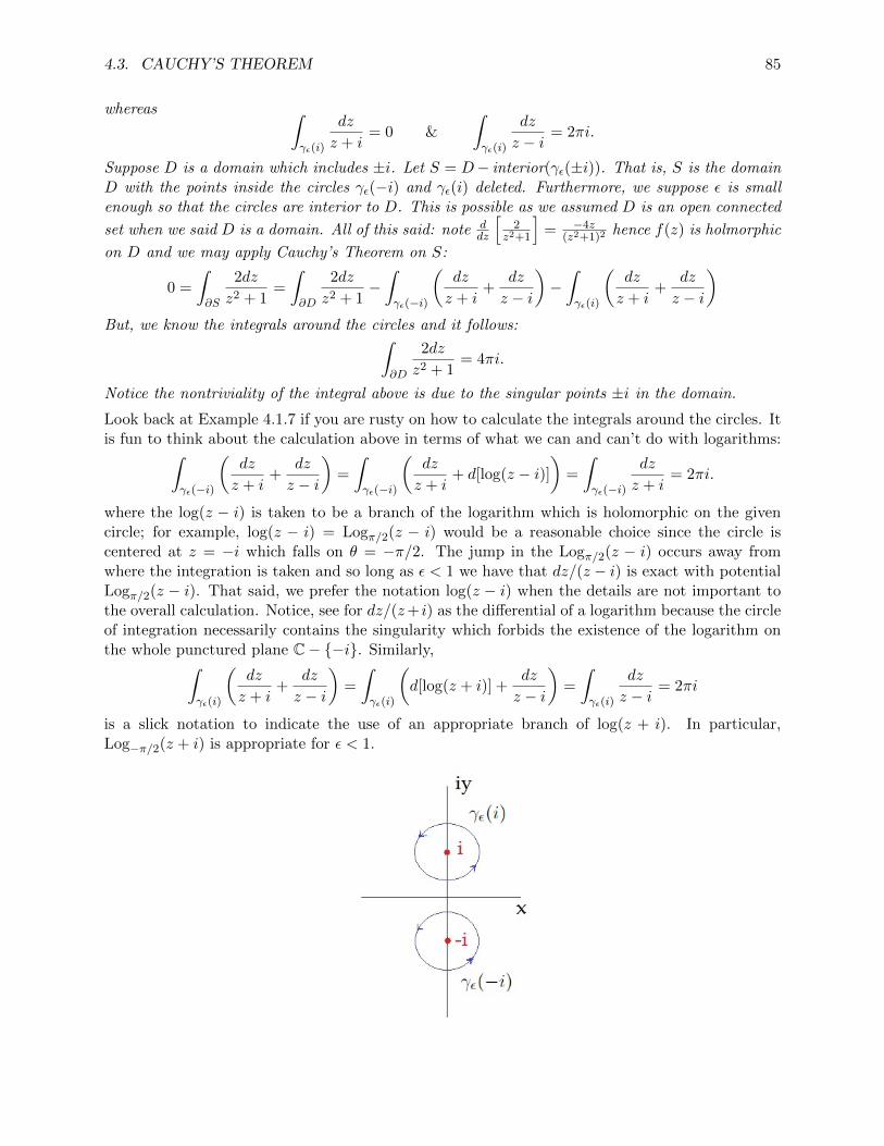
4.3. CAUCHY’S THEOREM 85
whereas ∫γε(i)
dz
z + i= 0 &
∫γε(i)
dz
z − i= 2πi.
Suppose D is a domain which includes ±i. Let S = D− interior(γε(±i)). That is, S is the domainD with the points inside the circles γε(−i) and γε(i) deleted. Furthermore, we suppose ε is smallenough so that the circles are interior to D. This is possible as we assumed D is an open connected
set when we said D is a domain. All of this said: note ddz
[2
z2+1
]= −4z
(z2+1)2hence f(z) is holmorphic
on D and we may apply Cauchy’s Theorem on S:
0 =
∫∂S
2dz
z2 + 1=
∫∂D
2dz
z2 + 1−∫γε(−i)
(dz
z + i+
dz
z − i
)−∫γε(i)
(dz
z + i+
dz
z − i
)But, we know the integrals around the circles and it follows:∫
∂D
2dz
z2 + 1= 4πi.
Notice the nontriviality of the integral above is due to the singular points ±i in the domain.
Look back at Example 4.1.7 if you are rusty on how to calculate the integrals around the circles. Itis fun to think about the calculation above in terms of what we can and can’t do with logarithms:∫
γε(−i)
(dz
z + i+
dz
z − i
)=
∫γε(−i)
(dz
z + i+ d[log(z − i)]
)=
∫γε(−i)
dz
z + i= 2πi.
where the log(z − i) is taken to be a branch of the logarithm which is holomorphic on the givencircle; for example, log(z − i) = Logπ/2(z − i) would be a reasonable choice since the circle iscentered at z = −i which falls on θ = −π/2. The jump in the Logπ/2(z − i) occurs away fromwhere the integration is taken and so long as ε < 1 we have that dz/(z − i) is exact with potentialLogπ/2(z − i). That said, we prefer the notation log(z − i) when the details are not important tothe overall calculation. Notice, see for dz/(z+ i) as the differential of a logarithm because the circleof integration necessarily contains the singularity which forbids the existence of the logarithm onthe whole punctured plane C− {−i}. Similarly,∫
γε(i)
(dz
z + i+
dz
z − i
)=
∫γε(i)
(d[log(z + i)] +
dz
z − i
)=
∫γε(i)
dz
z − i= 2πi
is a slick notation to indicate the use of an appropriate branch of log(z + i). In particular,Log−π/2(z + i) is appropriate for ε < 1.

86 CHAPTER IV. COMPLEX INTEGRATION AND ANALYTICITY
4.4 The Cauchy Integral Formula
Once again, when we assume holomorphic on a domain we also add the assumption of continuityof f ′(z) on the domain. Gamelin assumes continuity of f ′(z) when he says f(z) is analytic on D.As I have mentioned a few times now, we show in Section 4.7 that f(z) holomorphic on a domainautomatically implies that f ′(z) is continuous. This means we can safely delete the assumption ofcontinuity of f ′(z) once we understand Goursat’s Theorem.
The theorem below is rather surprising in my opinion.
Theorem 4.4.1. Cauchy’s Integral Formula (m = 0): let D be a bounded domain with piecewisesmooth boundary ∂D. If f(z) is holomorphic with continuous f ′(z) on D and f(z), f ′(z) extendcontinuously to ∂D then for each z ∈ D,
f(z) =1
2πi
∫∂D
f(w)
w − zdw
Proof: Assume the preconditions of the theorem. Fix a point z ∈ D. Note D is open hence z isinterior thus we are free to choose ε > 0 for which {w ∈ C | |w − z| < ε} ⊆ D. Define:
Dε = D − {w ∈ C | |w − z| ≤ ε}
Observe the boundary of Dε consists of the outer boundary ∂D and the circle γ−ε which is |w−z| = ε
given CW-orientation; ∂Dε = ∂D ∪ γ−ε . Further, observe g(w) = f(w)w−z is holomorphic as
g′(w) =f ′(w)
w − z− f(w)
(w − z)2
and g′(w) continuous on Dε and g(w), g′(w) both extend continuously to ∂Dε as we have assumedfrom the outset that f(w), f ′(w) extend likewise. We obtain from Cauchy’s Theorem 4.3.2 that:∫
∂Dε
f(w)
w − zdw = 0 ⇒
∫∂D
f(w)
w − zdw +
∫γ−ε
f(w)
w − zdw = 0.
However, if γ+ε denotes the CCW-oriented circle, we have
∫γ−ε
f(w)w−z dw = −
∫γ+ε
f(w)w−z dw hence:∫
∂D
f(w)
w − zdw =
∫γ+ε
f(w)
w − zdw
The circle γ+ε has w = z + εeiθ for 0 ≤ θ ≤ 2π thus dz = iεeiθdθ and we calculate:∫γ+ε
f(w)
w − zdw =
∫ 2π
0
f(z + εeiθ)
εeiθiεeiθdθ = 2πi
∫ 2π
0f(z + εeiθ)
dθ
2π= 2πif(z).
In the last step we used the Mean Value Property given by Theorem 3.4.2. Finally, solve for f(z)to obtain the desired result. �
We can formally derive the higher-order formulae by differentiation:
f ′(z) =1
2πi
d
dz
∫∂D
f(w)
w − zdw =
1
2πi
∫∂D
d
dz
[f(w)
w − z
]dw =
1!
2πi
∫∂D
f(w)
(w − z)2dw

4.4. THE CAUCHY INTEGRAL FORMULA 87
Differentiate once more,
f ′′(z) =1
2πi
d
dz
∫∂D
f(w)
(w − z)2dw =
1
2πi
∫∂D
d
dz
[f(w)
(w − z)2
]dw =
2!
2πi
∫∂D
f(w)
(w − z)3dw
continuing, we would arrive at:
f (m)(z) =m!
2πi
∫∂D
f(w)
(w − z)m+1dw
which is known as Cauchy’s generalized integral formula. Note that 0! = 1 and f (0)(z) = f(z)hence Theorem 4.4.1 naturally fits into the formula above.
It is probably worthwhile to examine a proof of the formulas above which is not based on differen-tiating under the integral. The arguments below show that our formal derivation above were valid.In the case m = 1 the needed algebra is simple enough:
1
w − (z +4z)− 1
w − z=
4z(w − (z +4z))(w − z)
.
Then, appealing to the m = 0 case to write the functions as integrals:
f(z +4z)− f(z)
4z=
1
2πi4z
∫∂D
1
w − (z +4z)dw +
1
2πi4z
∫∂D
1
w − zdw
=1
2πi4z
∫∂D
[1
w − (z +4z)− 1
w − z
]f(w) dw
=1
2πi
∫∂D
f(w)
(w − (z +4z))(w − z)dw.
Finally, as 4z → 0 we find f ′(z) = 12πi
∫∂D
f(w)(w−z)2 dw. We assume that the limiting process 4z → 0
can be interchanged with the integration process. Gamelin comments this is acceptable due to theuniform continuity of the integrand.
We now turn to the general case, assume Cauchy’s generalized integral formula holds for m − 1.We need to make use of the binomial theorem:
((w − z) +4z)m = (w − z)m −m(w − z)m−14z +m(m− 1)
2(w − z)m−2(4z)2 + · · ·+ (4z)m
Clearly, we have ((w − z) +4z)m = (w − z)m −m(w − z)m−14z + g(z, w)(4z)2 It follows that:
1
(w − (z +4z))m− 1
(w − z)m=m(w − z)m−14z + g(z, w)(4z)2
(w − (z +4z))m(w − z)m
=m4z
(w − (z +4z))(w − z)m.+
g(z, w)(4z)2
(w − (z +4z))m(w − z)m
Apply the induction hypothesis to obtain the integrals below:f (m−1)(z +4z)− f (m−1)(z)
4z=
=(m− 1)!
2πi4z
∫∂D
f(w)
(w − (z +4z))mdw +
(m− 1)!
2πi4z
∫∂D
f(w)
(w − z)mdw
=(m− 1)!
2πi4z
∫∂D
[m4z
(w − (z +4z))(w − z)m.+
g(z, w)(4z)2
(w − (z +4z))m(w − z)m
]f(w) dw
=m!
2πi
∫∂D
f(w)dw
(w − (z +4z))(w − z)m.+
(m− 1)!
2πi
∫∂D
g(z, w)4zf(w)dw
(w − (z +4z))m(w − z)m.

88 CHAPTER IV. COMPLEX INTEGRATION AND ANALYTICITY
As 4z → 0 we see the right integral vanishes and the left integral has a denominator which tendsto (w − z)m+1 hence, by the definition of the m-th derivative,
f (m)(z) =m!
2πi
∫∂D
f(w)dw
(w − z)m+1
The arguments just given provide proof of the following theorem:
Theorem 4.4.2. Cauchy’s Generalized Integral Formula (m ∈ N∪ {0}): let D be a boundeddomain with piecewise smooth boundary ∂D. If f(z) is holomorphic with continuous f ′(z) on Dand f(z), f ′(z) extend continuously to ∂D then for each z ∈ D,
f (m)(z) =m!
2πi
∫∂D
f(w)
(w − z)m+1dw
Often we need to use the theorem above with the role of z as the integration variable. For example:
f (m)(zo) =m!
2πi
∫∂D
f(z)
(z − zo)m+1dz
from which we obtain the useful identity:
∫∂D
f(z)
(z − zo)m+1dz =
2πif (m)(zo)
m!
This formula allows us to calculate many difficult integrals by simple evaluation of an approrpriatederivative. That said, we do improve on this result when we uncover the technique of residues laterin the course. Think of this as an intermediate step in our calculational maturation.
Example 4.4.3. Let the integral below be taken over the CCW-oriented curve |z| = 1:∮|z|=2
sin(2z)
(z − i)6dz =
2πi
5!
d5
dz5
∣∣∣∣z=i
sin(2z) =2πi
5 · 4 · 3 · 2(−32 cos(2i)) =
−8πi cosh(2)
15.
Example 4.4.4. Notice that z4 + i = 0 for z ∈ (−i)1/4 =(e−iπ/2
)1/4= e−iπ/8{1, i,−1,−i} hence
z4 + i = (z − e−iπ/8)(z − ie−iπ/8)(z + e−iπ/8)(z + ie−iπ/8). Consider the circle |z − 1| = 1 (blue).The dotted circle is the unit-circle and the intersection near ie−iπ/8 is at θ = π/3 which is roughlyas illustrated.
The circle of integration below encloses the principal root (red), but not the other three non-principalfourth roots of −i(green). Consequently, we apply Cauchy’s integral formula based on the divergence

4.5. LIOUVILLE’S THEOREM 89
of the principal root:∮|z−1|=1
dz
z4 + i=
∮|z−1|=1
dz
(z − e−iπ/8)(z − ie−iπ/8)(z + e−iπ/8)(z + ie−iπ/8)
=2πi
(z − ie−iπ/8)(z + e−iπ/8)(z + ie−iπ/8)
∣∣∣∣z=e−iπ/8
=2πi
(e−iπ/8 − ie−iπ/8)(e−iπ/8 + e−iπ/8)(e−iπ/8 + ie−iπ/8)
=2πi
e−3iπ/8(1− i)(1 + 1)(1 + i)
=πi
2e3iπ/8.
Of course, you could simplify the answer further and present it in Cartesian form.
Some of the most interesting applications involve integrations whose boundaries are allowed to ex-pand to infinity. We saw one such example in Problem 53 which was #1 from IV.3 in Gamelin. Thekey in all of our problems is that we must identify the divergent points for the integrand. Providedthey occur either inside or outside the curve we proceed as we have shown in the examples above.We do study divergences on contours later in the course, there are some precise results which areknown for improper integrals of that variety6
Finally, one last point:
Corollary 4.4.5. If f(z) is holomorphic with continuous derivative f ′(z) on a domain D then f(z)is infinitely complex differentiable. That is, f ′, f ′′, . . . all exist and are continuous on D.
The proof of this is that Cauchy’s integral formula gives us an explicit expression (which exists) forany possible derivative of f . There are no just once or twice continuously complex differentiablefunctions. You get one continuous derivative on a domain, you get infinitely many. Pretty gooddeal. Moreover, the continuity of the derivative is not even needed as we discover soon.
4.5 Liouville’s Theorem
It is our convention to say f(z) is holomorphic on a closed set D iff there exists an open setD containing D on which f(z) ∈ O(D). Consider a function f(z) for which f ′(z) exists and iscontinuous for z ∈ C such that |z − zo| ≤ ρ. In such a case Cauchy’s integral formula applies:
f (m)(zo) =m!
2πi
∫|z−zo|≤ρ
f(z)
(z − zo)m+1dz
We parametrize the circle by z = zo + ρeiθ for 0 ≤ θ ≤ 2π where dz = iρeiθdθ. Therefore,
f (m)(zo) =m!
2πi
∫ 2π
0
f(zo + ρeiθ)
(ρeiθ)m+1iρeiθdθ =
m!
2πρm
∫ 2π
0f(zo + ρeiθ)e−imθdθ
If we have |f(zo + ρeiθ)| ≤M for 0 ≤ θ ≤ 2π then the we find∣∣∣∣∫ 2π
0f(zo + ρeiθ)e−imθdθ
∣∣∣∣ ≤ ∫ 2π
0
∣∣∣f(zo + ρeiθ)e−imθ∣∣∣ dθ =
∫ 2π
0
∣∣∣f(zo + ρeiθ)∣∣∣ dθ ≤ 2πM.
The discussion above serves to justify the bound given below:
6in particular, see §V II.5 if you wish

90 CHAPTER IV. COMPLEX INTEGRATION AND ANALYTICITY
Theorem 4.5.1. Cauchy’s Estimate: suppose f(z) is holomorphic with continuous derivativeon a domain D then for any closed disk {z ∈ C | |z − zo| ≤ ε} ⊂ D on which |f(z)| ≤ M for allz ∈ C with |z − zo| = ρ we find ∣∣∣f (m)(zo)
∣∣∣ ≤ Mm!
ρm
Many interesting results flow from the estimate above. For example:
Theorem 4.5.2. Liouville’s Theorem: Suppose f(z) is holomorphic with continuous derivativeon C. If |f(z)| ≤M for all z ∈ C then f(z) is constant.
Proof: Assume f(z), f ′(z) are continuous on C and |f(z)| ≤M for all C. Let us consider the diskof radius R centered at zo. From Cauchy’s Estimate with m = 1 we obtain:
∣∣f ′(zo)∣∣ ≤ M
R.
Observe, as R → ∞ we find |f ′(zo)| → 0 hence f ′(zo) = 0. But, zo was an arbitrary point in Chence f ′(z) = 0 for all z ∈ C and as C is connected we find f(z) = c for all z ∈ C. �
We saw in the homework that this theorem allows a relatively easy proof of the FundamentalTheorem of Algebra. In addition, we were able to show that an entire function whose range missesa disk of values must be constant. As I mentioned in class, the take-away message here is simplythis: every bounded entire function is constant.
4.6 Morera’s Theorem
I think the central result of this section is often attributed to Goursat. More on that in the nextsection. Let us discuss what is presented in Gamelin. It is important to note that continuousdifferentiability of f(z) is not assumed as a precondition of the theorem.
Theorem 4.6.1. Morera’s Theorem: Let f(z) be a continuous function on a domain U . If∫∂R f(z)dz = 0 for every closed rectangle R contained in U with sides parallel to the coordinate
axes then f(z) is holomorphic with continuous f ′(z) in U .
Proof: the vanishing of the rectangular integral allows us to exchange the lower path between twovertices of a rectangle for the upper path:
It suffices to prove the theorem for a disk D with center zo where D ⊆ U7. Define:
F (z) =
∫γd(z)
f(w)dw
7do you understand why this is true and no loss of generality here?

4.6. MORERA’S THEOREM 91
where γd(z) = [xo+iyo, iyo+x]∪ [iyo+x, x+iy] where zo = xo+iyo and z = x+iy. To show F ′(z)exists we consider the difference: here 4z is a small enough displacement as to keep z +4z ∈ D,the calculation below is supported by the diagram which follows after:
F (z + 4z)− F (z) =
∫γd(z+4z)
f(w)dw −∫γd(z)
f(w)dw
=
∫γd(z+4z)
f(w)dw +
∫−γd(z)
f(w)dw
=
∫γu(z,z+4z)
f(w)dw ? .
Where −γd(z) denotes the reversal of γd(z). I plotted it as the red path below. The blue path isγd(z +4z). By the assumption of the theorem we are able to replace the sum of the blue and redpaths by the green path γu(z, z +4z).
Notice, f(z) is just a constant in the integral below hence:∫γu(z,z+4z)
f(z)dw = f(z)
∫ z+4z
zdw = f(z)w
∣∣∣∣z+4zz
= f(z)4z.
Return once more to ? and add f(z)− f(z) to the integrand:
F (z + 4z)− F (z) =
∫γu(z,z+4z)
[f(z) + f(w)− f(z)]dw
= f(z)4z +
∫γu(z,z+4z)
(f(w)− f(z)
)dw ? ?
Note L(γu(z, z +4z)) < 2|4z| and if we set M = sup{|f(w)− f(z)| | z ∈ γu(z, z +4z)} then theML-estimate provides ∣∣∣∣∣
∫γu(z,z+4z)
(f(w)− f(z)
)dw
∣∣∣∣∣ ≤ML < 2M |4z|
Rearranging ?? we find: ∣∣∣∣F (z + 4z)− F (z)
4z− f(z)
∣∣∣∣ ≤ 2M.
Notice that as 4z → 0 we have 2M → 0 hence F ′(z) = f(z) be the inequality above. Furthermore,we assumed f(z) continuous hence F ′(z) is continuous. Consequently F (z) is both holomorphicand possesses continuous derivative F ′(z) on D. Apply the Corollary 4.4.5 to Cauchy’s GeneralizedIntegral Formula to see that F ′′(z) = f ′(z) exists and is continuous. �

92 CHAPTER IV. COMPLEX INTEGRATION AND ANALYTICITY
4.7 Goursat’s Theorem
Let me begin with presenting Goursat’s Theorem as it appears in Gamelin:
Theorem 4.7.1. Goursat’s Theorem: (Gamelin Version) If f(z) is a complex-valued functionon a domain D such that
f ′(zo) = limz→zo
f(z)− f(zo)
z − zoexists at each point zo of D then f(z) is analytic on D.
Notice, in our langauge, the theorem above can be stated: If a function is holomorphic on a domainD then z → f ′(z) is continuous.
Proof: let R be a closed rectangle in D with sides parallel to the coordinate axes. Divide R into four
identical sub-rectangles and let R1 be the sub-rectangle for which∣∣∣∫∂R1
f(z)dz∣∣∣ is largest (among
the 4 sub-rectangles). Observe that∣∣∣∫∂R1
f(z)dz∣∣∣ ≥ 1
4
∣∣∫∂R f(z)dz
∣∣ or, equivalently,∣∣∫∂R f(z)dz
∣∣ ≤4∣∣∣∫∂R1
f(z)dz∣∣∣. Then, we subdivide R1 into 4 sub-rectangles and the rectangle with largest integral
R2. Continuing in this fashion we obtain a sequence of nested rectangles R ⊃ R1 ⊃ R2 ⊃ · · · ⊃Rn ⊃ · · · . It is a simple exercise to verify:∣∣∣∣∫
∂Rn
f(z)dz
∣∣∣∣ ≤ 4
∣∣∣∣∣∫∂Rn+1
f(z)dz
∣∣∣∣∣ ⇒∣∣∣∣∫∂Rf(z)dz
∣∣∣∣ ≤ 4n∣∣∣∣∫∂Rn
f(z)dz
∣∣∣∣ ? .
The subdivision process is illustrated below:
As n → ∞ it is clear that the sequence of nested rectangles converges to a point zo ∈ R. Fur-thermore, if L is the length of the perimeter of R then L/2n is the length of ∂Rn. As f(z) iscomplex-differentiable at zo we know for each z ∈ Rn there must exist an εn such that∣∣∣∣f(z)− f(zo)
z − zo− f ′(zo)
∣∣∣∣ ≤ εnhence ∣∣f(z)− f(zo)− f ′(zo)(z − zo)
∣∣ ≤ εn|z − zo| ≤ 2εnL/2n ? ?.
The last inequality is very generous since zo, z ∈ Rn surely implies they are closer than the perimeterL/2n apart. Notice, the function g(z) = f(zo) + f ′(zo)(z − zo) has primitive G(z) = f(zo)z +f ′(zo)(z
2/2− zzo) on Rn hence8∫∂Rn
g(z)dz = 0. Subtracting this zero is crucial:∣∣∣∣∫∂Rn
f(z)dz
∣∣∣∣ =
∣∣∣∣∫∂Rn
[f(z)− f(zo)− f ′(zo)(z − zo)
]dz
∣∣∣∣ ≤ (2εnL/2n)(L/2n) =
2L2εn4n
.
8this application of Cauchy’s Theorem does not beg the question by assuming continuity of g′(z)

4.8. COMPLEX NOTATION AND POMPEIU’S FORMULA 93
where we applied the ML-estimate by ?? and L(∂Rn) = L/2n. Returning to ?,∣∣∣∣∫∂Rf(z)dz
∣∣∣∣ ≤ 4n∣∣∣∣∫∂Rn
f(z)dz
∣∣∣∣ ≤ 4n · 2L2εn4n
= 2L2εn.
Finally, as n → 0 we have εn → 0 thus it follows∫∂R f(z)dz = 0. But, this shows the integral
around an arbitrary rectangle in D is zero hence by Morera’s Theorem 4.6.1 we find f(z) is holo-morphic with continuous f ′(z) on D. �
We now see that holomorphic functions on a domain are indeed analytic (as defined by Gamelin).
4.8 Complex Notation and Pompeiu’s Formula
My apologies, it seems I have failed to write much here. I have many things to say, some of themI said in class. Recently, we learned how to generalize the idea of this section to nearly arbitraryassociative algebras. More on that somewhere else.

94 CHAPTER IV. COMPLEX INTEGRATION AND ANALYTICITY

Chapter V
Power Series
A power series is simply a polynomial without end. But, this begs questions. What does ”withoutend” mean? How can we add, subtract, multiply and divide things which have no end? In thischapter we give a careful account of things which go on without end.
History provides examples of the need for caution1. For example, even Cauchy wrongly assertedin 1821 that an infinite series of continuous functions was once more continuous. In 1826 Abel2
provided a counter-example and in the years to follow the concept of uniform convergence wasinvented to avoid such blunders. Abel had the following to say about the state of the theory as hesaw it: from page 114 of [R91]
If one examines more closely the reasoning which is usually employed in the treatmentof infinite series, he will find that by and large it is unsatisfactory and that the numberof propositions about infinite series which can be regarded as rigorously confirmed issmall indeed
The concept of uniform convergence is apparently due to the teacher of Weierstrauss. ChristophGudermann wrote in 1838: ”it is a fact worth noting that... the series just found have all thesame convergence rate”. Weierstrauss used the concept of uniform convergence throughout hiswork. Apparently, Seidel and Stokes independently in 1848 and 1847 also used something akin touniform convergence of a series, but the emminent British mathematician G.H Hardy gives creditto Weierstrauss:
Weierstrauss’s discovery was the earliest, and he alone fully realized its far-reachingimportance as one of the fundamental ideas of analysis
It is fun to note Cauchy’s own view of his 1821 oversight. In 1853 in the midst of a work whichused and made significant contributions to the theory of uniformly convergent series, he wrote thatit is easy to see how one should modify the statement of the theorem. See page 102 of [R91] formore details as to be fair to Cauchy.
In this chapter, we study convergence of sequence and series. Ultimately, we find how power serieswork in the complex domain. The results are surprisingly simple as we shall soon discover. Mostimportantly, we introduce the term analytic and see in what sense it is equivalent to our termholomorphic. Obviously, we differ from Gamelin on this point of emphasis.
1the facts which follow here are taken from [R91] pages 96-98 primarily2did work on early group theory, we name commutative groups Abelian groups in his honor
95

96 CHAPTER V. POWER SERIES
5.1 Infinite Series
We discussed and defined complex sequences in Chapter 2. See Definition 2.1.1. We now discussseries of complex numbers. In short, a complex series is formed by adding the terms in somesequence of complex numbers:
∞∑n=0
zn = zo + z1 + z2 + · · ·
If this sum exists as a complex number then the series is convergent whereas if the sum above doesnot converge then the series is said to be divergent. The convergence (or divergence) of the seriesis described precisely by the convergence (or divergence) of the sequence of partial sums:
Definition 5.1.1. Let an ∈ C for each n ∈ N ∪ {0} then we define
∞∑j=0
aj = limn→∞
n∑j=0
aj .
If limn→∞∑n
j=0 aj = S ∈ C then the series ao + a1 + · · · is said to converge to S.
The linearity theorems for sequences induce similar theorems for series. In particular, Theorem2.1.3 leads us to:
Theorem 5.1.2. Let c ∈ C,∑aj = A and
∑bj = B then
∑(aj + bj) = A+B and
∑caj = cA;∑
(aj + bj) =∑
aj +∑
bj additivity of convergent sums∑cbj = c
∑bj homogeneity of convergent sums
Proof: let Sn =∑n
j=0 aj and Tn =∑n
j=0 bj . We are given, from the definition of convergent series,that these partial sums converge; Sn → A and Tn → B as n→∞. Consider then,
n∑j=0
(aj + cbj) =n∑j=0
aj + cn∑j=0
bj
Thus, the sequence of partial sums for∑∞
j=0(aj + cbj) is found to be Sn + cTn. Apply Theorem2.1.3 and conclude Sn + cTn → A+ cB as n→∞. Therefore,
∞∑j=0
(aj + cbj) =∞∑j=0
aj + c∞∑j=0
bj .
If we set c = 1 we obtain additivity, if we set A = 0 we obtain homogeneity. �
I offered a proof for series which start at j = 0, but, it ought to be clear the same holds for serieswhich start at any particular j ∈ Z.
Let me add a theorem which is a simple consequence of Theorem 2.1.10 applied to partial sums:
Theorem 5.1.3. Let xk, yk ∈ R then∑xk + iyk converges iff
∑xk and
∑yk converge. Moreover,
in the convergent case,∑xk + iyk =
∑xk + i
∑yk.

5.1. INFINITE SERIES 97
Series of real numbers enjoy a number of results which stem from the ordering of the real numbers.The theory of series with non-negative terms is particularly intuitive. Suppose ao, a1, · · · > 0 then{ao, ao + a1, ao + a1 + a2, . . . } is a monotonically increasing sequence. Recall Theorem 2.1.5 whichsaid that a monotonic sequence converged iff it was bounded.
Theorem 5.1.4. If 0 ≤ ak ≤ rk, and if∑rk converges, then
∑ak converges, and
∑ak ≤
∑rk.
Proof: obviously ak, rk ∈ R by the condition 0 ≤ ak ≤ rk. Observe∑n+1
k=0 rk = rn+1 +∑n
k=0 rkhence
∑n+1k=0 rk ≥
∑nk=0 rk. Thus the sequence of partial sums of
∑rk is increasing. Since
∑rk
converges it follows that the convergent sequence of partial sums is bounded. That is, there existsM ≥ 0 such that
∑nk=0 rk ≤ M for all n ∈ N ∪ {0}. Notice ak ≤ rk implies
∑nk=0 ak ≤
∑nk=0 rk.
Therefore,∑n
k=0 ak ≤ M . Observe ak ≥ 0 implies∑n
k=0 ak is increasing by the argument wealready offered for
∑nk=0 rk. We find
∑nk=0 ak is a bounded, increasing sequence of non-negative
real numbers thus limn→∞∑n
k=0 ak = A ∈ R by Theorem 2.1.5. Finally, we appeal to part ofthe sandwhich theorem for real sequences, if cn ≤ dn for all n and both cn and dn converge thenlimn→∞ cn ≤ limn→∞ dn. Think of cn =
∑nk=0 ak and dn =
∑nk=0 rk. Note
∑nk=0 ak ≤
∑nk=0 rk
implies limn→∞∑n
k=0 ak ≤ limn→∞∑n
k=0 rk. The theorem follows. �
Can you appreciate the beauty of how Gamelin discusses convergence and proofs ? Compare theproof I give here to his paragraph on page 130-131. His prose captures the essential details of whatI wrote above without burying you in details which obscure. In any event, I will continue to adduglified versions of Gamelin’s prose in this chapter. I hope that by seeing both your understandingis fortified.
We return to the study of complex series once more. Suppose aj ∈ C in what follows. The definitionof a finite sum is made recursively by
∑0j=0 aj = ao and for n ≥ 1:
n∑j=0
aj = an +n−1∑j=0
aj .
Notice this yields:
an =
n∑j=0
aj −n−1∑j=0
aj .
Suppose∑∞
j=0 aj = S ∈ C. Observe, as n → ∞ we see that∑n
j=0 aj −∑n−1
j=0 aj → S − S = 0.Therefore, the condition an → 0 as n→∞ is a necessary condition for convergence of ao+a1+· · · .
Theorem 5.1.5. If∑∞
j=0 aj converges then aj → 0 as j →∞.
Of course, you should recall from calculus that the criteria above is not sufficient for convergenceof the series. For example, 1 + 1/2 + 1/3 + · · · diverges despite the fact 1/n→ 0 as n→∞.
I decided to elevate Gamelin’s example on page 131 to a proposition.
Proposition 5.1.6. Let zj ∈ C for j ∈ N ∪ {0}.
If |z| < 1 then∞∑j=0
zn =1
1− z. If |z| ≥ 1 then
∞∑j=0
zn diverges.

98 CHAPTER V. POWER SERIES
Proof: if |z| ≥ 1 then the n-th term test shows the series diverges. Suppose |z| < 1. Consider,
Sn = 1 + z + z2 · · ·+ zn ⇒ zSn = z + z2 + · · ·+ zn + zn+1
and we find Sn − zSn = 1− zn+1 thus (1− z)Sn = 1− zn+1 and derive:
Sn =1− zn+1
1− z
This is a rare and wonderful event that we were able to explicitly calculate the n-th partial sumwith such small effort. Note |z| < 1 implies |z|n+1 → 0 as n→∞. Therefore,
∞∑j=0
zn = limn→∞
1− zn+1
1− z=
1
1− z. �
Definition 5.1.7. A complex series∑ak is said to converge absolutely if
∑|ak| converges.
Notice that |ak| denotes the modulus of ak. In the case ak ∈ R this reduces to the usual3 definitionof absolute convergence since the modulus is merely the absolute value function in that case. Ifyou’d like to see a proof of absolute convergence in the real case, I recommend page 82 of [J02].The proof there is based on parsing the real series into non-negative and negative terms. We haveno such dichotomy to work with here so something else must be argued.
Theorem 5.1.8. If∑ak is absolutely convergent then
∑ak converges and
∣∣∣∑ ak
∣∣∣ ≤∑ |ak|.
Proof: assume∑|ak| converges. Let ak = xk + iyk where xk, yk ∈ R. Observe:
|ak| =√x2k + y2
k ≥√x2k = |xk| & |ak| ≥ |yk|.
Thus, |xk| ≤ |ak| hence by comparison test the series∑|xk| converges with
∑|xk| ≤
∑|ak|. Like-
wise, |yk| ≤ |ak| hence by comparison test the series∑|yk| converges with
∑|yk| ≤
∑|ak|. Recall
that absolute convergence of a real series implies convergence hence∑xk and
∑yk exist. Theorem
5.1.3 allows us to conclude∑xk + iyk =
∑ak converges. �
Given that I have used the absolute convergence theorem for real series I think it is appropriate tooffer the proof of that theorem since many of you may either have never seen it, or at a minimum,have forgotten it. Following page 82 of [J02] consider a real series
∑∞n=0 xn. We define:
pn =
{xn if xn ≥ 0
0 if xn < 0& qn =
{0 if xn ≥ 0
−xn if xn < 0
Notice xn = pn − qn. Furthermore, notice pn, qn are non-negative terms. Observe
p0 + p1 + · · ·+ pn ≤ |xo|+ |x1|+ · · ·+ |xn|
Hence∑|xn| converging implies
∑pn converges by Comparison Theorem 5.1.4 and
∑pn ≤
∑|xn|.
Likewise,q0 + q1 + · · ·+ qn ≤ |xo|+ |x1|+ · · ·+ |xn|
3in the sense of second semester calculus where you probably first studied series

5.2. SEQUENCES AND SERIES OF FUNCTIONS 99
Hence∑|xn| converging implies
∑qn converges by Comparison Theorem 5.1.4 and
∑qn ≤
∑|xn|.
But, then∑xn =
∑(pn − qn) =
∑pn −
∑qn by Theorem 5.1.2. Finally, notice
x0 + x1 + · · ·+ xn ≤ |x0|+ |x1|+ · · ·+ |xn|
thus as n → ∞ we obtain∑xn ≤
∑|xn|. This completes the proof that absolute convergence
implies convergence for series with real terms.
I challenge you to see that my proof here is really not that different from what Gamelin wrote4.
Example 5.1.9. Consider |z| < 1. Proposition 5.1.6 applies to show∑zj is absolutely convergent
by direct calculation and: ∣∣∣∣ 1
1− z
∣∣∣∣ =
∣∣∣∣∣∣∞∑j=0
zj
∣∣∣∣∣∣ ≤∞∑j=0
|z|j =1
1− |z|.
Following Gamelin,
1
1− z−
n∑k=0
zk =∞∑k=0
zk −n∑k=0
zk =∞∑
k=n+1
zk = zn+1∞∑k=0
zk =zn+1
1− z.
Therefore, ∣∣∣∣∣ 1
1− z−
n∑k=0
zk
∣∣∣∣∣ =|z|n+1
|1− z|≤ |z|
n+1
1− |z|.
The inequality above gives us a bound on the error for the n-th partial sum of the geometric series.
If you are interested in the history of absolute convergence, you might look at pages 29-30 of [R91]where he describes briefly the influence of Cauchy, Dirichlet and Riemann on the topic. It wasRiemann who proved that a series which converges but, does not converge absolutely, could berearranged to converge to any value in R.
5.2 Sequences and Series of Functions
A sequence of functions on E ⊆ C is an assignment of a function on E for each n ∈ N ∪ {0}.Typically, we denote the sequence by {fn} or simply by fn. In addition, although we are ultimatelyinterested in the theory of sequences of complex functions, I will give a number of real examples toillustrate the subtle issues which arise in general.
Definition 5.2.1. A sequence of functions fn on E is said to pointwise converge to f iflimn→∞ fn(z) = f(z) for all z ∈ E.
You might be tempted to suppose that if each function of the sequence is continuous and the limitexists then surely the limit function is continuous. Well, you’d be wrong:
Example 5.2.2. Let n ∈ N ∪ {0} and define fn(x) = xn for x ∈ [0, 1]. We can calculate the limitfunction:
f(x) = limn→∞
xn =
{0 if 0 ≤ x < 1
1 if x = 1
4Bailu, notice the proof I give here easily extends to an associative algebra

100 CHAPTER V. POWER SERIES
Notice, fn is continuous for each n ∈ N, but, the limit function f is not continuous. In particular,you can see we cannot switch the order of the limits below:
0 = limx→1−
(limn→∞
xn)6= lim
n→∞
(limx→1−
xn)
= 1
To guarantee the continuity of the limit function we need a stronger mode of convergence. FollowingGamelin (and a host of other analysis texts) consider:
Example 5.2.3. We define a sequence for which each function gn makes a triangular tent of slope±n2 from x = 0 to x = 2/n. In particular, for n ∈ N define:
gn(x) =
n2x if 0 ≤ x < 1/n
2n− n2x if 1/n ≤ x ≤ 2/n
0 if 2/n ≤ x ≤ 1
Notice, ∫ 1/n
0n2xdx = n2 (1/n)2
2=
1
2
and ∫ 2/n
1/n(2n− n2x)dx = 2n(2/n− 1/n)− n2
2[(2/n)2 − (1/n)2] = 2− 3
2=
1
2.
Therefore,∫ 1
0 gn(x) dx = 1 for each n ∈ N. However, as n → ∞ we find gn(x) → 0 for eachx ∈ [0, 1]. Observe:
1 = limn→∞
∫ 1
0gn(x) dx 6=
∫ 1
0limn→∞
gn(x) dx = 0.
To guarantee the integral of the limit function is the limit of the integrals of the sequence we needa stronger mode of convergence. Here I break from Gamelin and add one more example.
Example 5.2.4. For each n ∈ N define fn(x) = xn/n for 0 ≤ x ≤ 1. Notice that limn→∞ xn/n = 0
for each x ∈ [0, 1]. Furthermore, limx→a xn/n = an/n for each a ∈ [0, 1] where we use one-sided
limits at a = 0+, 1−. It follows that:
limn→∞
limx→a
xn
n= lim
n→∞
an
n= 0
likewise,
limx→a
limn→∞
xn
n= lim
x→a0 = 0
Thus, the limit n→∞ and x→ a commute for this sequence of functions.
The example above shows us there is hope for the limit of a sequence of continuous function to becontinuous. Perhaps we preserve derivatives under the limit ? Consider:
Example 5.2.5. Once more study fn(x) = xn/n for 0 ≤ x ≤ 1. Notice dfndx = xn−1. However, this
is just the sequence we studied in Example 5.2.2,
limn→∞
dfndx
=
{0 if 0 ≤ x < 1
1 if x = 1⇒ lim
x→1−limn→∞
dfndx
= limx→1−
(0) = 0.

5.2. SEQUENCES AND SERIES OF FUNCTIONS 101
On the other hand,
limx→1−
dfndx
= limx→1−
xn−1 = 1 ⇒ limn→∞
limx→1−
dfndx
= limn→∞
(1) = 1.
Therefore, the limit of the sequence of derivatives is not the derivative of the limit function.
The examples above lead us to define a stronger type of convergence which preserves continuityand integrals to the limit. However, in the real case, differentiation is still subtle.
The standard definition of uniform convergence is given below:5
Definition 5.2.6. Let {fn} be a sequence of functions on E. Let f be a function on E. We say{fn} converges uniformly to f if for each ε > 0 there exists an N ∈ N such that n > N implies|fn(x)− f(x)| < ε for all x ∈ E.
This is not quite Gamelin’s presentation. Instead, from page 134, Gamelin says:
We say a sequence of functions {fj} converges uniformly to f on E if |fj(x)−f(x)| ≤εj for all x ∈ E where εj → 0 as j → ∞. We call εj the worst-case estimator ofthe difference fj(x) − f(x) and usually take εj to be the supremum (maximum) of|fj(x)− f(x)| over x ∈ E,
εj = supx∈E|fj(x)− f(x)|.
Very well, are these definitions of uniform convergence equivalent? For a moment, let us define theuniform convergence of Gamelin as G-uniform convergence whereas that given in the Definition5.2.6 defines S-uniform convergence. The question becomes:
Can we show a sequence of functions {fn} on E is S-uniformly convergent to f on Eiff the sequence of functions is G-uniformly convergent to f on E ?
This seems like an excellent homework question, so, I will merely assert it’s verity for us here:
Theorem 5.2.7. Let {fn} be a sequence of functions on E. Then {fn} is S-uniformly convergentto f on E if and only if {fn} is G-uniformly convergent to f on E.
Proof: by trust in Gamelin, or as is my preference, your homework. �
The beautiful feature of Gamelin’s definition is that it gives us a method to calculate the worst-case estimator. We merely need to find the maximum difference between the n-th function in thesequence and the limit function over the given domain of interest (E).
If you think about it, the supremum gives you the best worst-case estimator. Let me explain, ifεj has |fj(z) − f(z)| ≤ εj for all z ∈ E then εj is an upper bound on |fj(z) − f(z)|. But, thesupremum is the least upper bound hence |fj(w) − f(w)| ≤ supz∈E |fj(z) − f(z)| ≤ εj for allw ∈ E. This simple reasoning shows us that when the supremum exists and we may use it as aworst-case estimator provided we also know supz∈E |fj(z) − f(z)| → 0 as j → ∞. On the otherhand, if no supremum exists or if the supremum does not go to zero as j → ∞ then we have nohope of finding a worst case estimator.
5for instance, see page 246 of [J02].
102 CHAPTER V. POWER SERIES
The paragraph above outlines the logic used in the paragraphs to follow.
In Example 5.2.2 we had fn(x) = xn for x ∈ [0, 1] pointwise converged to f(x) =
{0 if 0 ≤ x < 1
1 if x = 1
from which we may calculate6 supx∈[0,1] |xn−f(x)| = 1. Therefore, it is not possible to find εn → 0.In Gamelin’s terminology, the worst-case estimator is 1 hence this sequence is not uniformly con-vergent to f(x) on [0, 1].
In Example 5.2.3 we had
gn(x) =
n2x if 0 ≤ x < 1/n
2n− n2x if 1/n ≤ x ≤ 2/n
0 if 2/n ≤ x ≤ 1
which is point-wise convergent to g(x) = 0 for x ∈ [0, 1]. The largest value attained by gn(x) isfound at x = 1/n where
gn(1/n) = n2(1/n) = n
Therefore,
supx∈[0,1]
|gn(x)− g(x)| = n.
Therefore, the convergence of {gn} to g is not uniform on [0, 1].
Next, consider Example 5.2.4 where we noted that fn(x) = xn/n converges pointwise to f(x) = 0on [0, 1]. In this case it is clear that fn(1) = 1/n is the largest value attained by fn(x) on [0, 1]hence:
supx∈[0,1]
|fn(x)− f(x)| = 1/n = εn → 0 as n→∞.
Hence {xn/n} converges uniformly to f(x) = 0 on [0, 1]. Apparently, continuity is preserved underuniform convergence. On the other hand, Example 5.2.5 shows us that, for real functions, deriva-tives need not be preserved in a uniformly convergent limit.
We now present the two major theorems about uniformly convergent sequences of functions.
Theorem 5.2.8. Let {fj} be a sequence of complex-valued functions on E ⊆ C. If each fj iscontinuous on E and if {fj} converges uniformly to f on E then f is continuous on E.
Proof: let ε > 0. By uniform convergence, there exists N ∈ N for which
|fN (z)− f(z)| < ε
3?
for all z ∈ E. However, by continuity of fN at z = a there exists δ > 0 such that 0 < |z − a| < δimplies
|fN (z)− fN (a)| < ε
3? ?.
6sometimes the supremum is also known as the least upper bound, it is the smallest possible upper bound on theset in question. In this case, 1 is not attained in the set, but numbers arbitrary close to 1 are attained. Technically,this set has no maximum which is why the parenthetical comment in Gamelin suggesting supremum and maximumare synonyms is sometimes not helpful.

5.2. SEQUENCES AND SERIES OF FUNCTIONS 103
We claim f(z) is continuous at z = a by the same choice of δ. Consider, for 0 < |z − a| < δ,
|f(z)− f(a)| = |f(z)− fN (z) + fN (z)− fN (a) + fN (a)− f(a)|≤ |fN (z)− f(z)|+ |fN (z)− fN (a)|+ |fN (a)− f(a)|
≤ ε
3+ε
3+ε
3= ε
where I have used ?? for the middle term and ? for the left and rightmost terms. Thus limz→a f(z) =f(a) and as a ∈ E was arbitrary we have shown f continuous on E. �
I followed the lead of [J02] page 246 where they offer the same proof for an arbitary metric space.
Theorem 5.2.9. Let γ be a piecewise smooth curve in the complex plane. If {fj} is a sequence ofcontinuous complex-valued functions on γ, and if {fj} converges uniformly to f on γ then
∫γ fj(z)dz
converges to∫γ f(z)dz.
Proof: let εj be the worst-case estimator for fj − f on γ then |fj(z) − f(z)| ≤ εj for all z ∈ [γ].Let γ have length L and apply the ML-estimate:∣∣∣∣∫
γ(fj(z)− f(z))dz
∣∣∣∣ ≤ εjL.Thus, as j →∞ we find
∣∣∣∫γ fj(z)dz − ∫γ f(z)dz∣∣∣→ 0. �
This theorem is also true in the real case as you may read on page 249 of [J02]. However, thatproof requires we understand the real analysis of integrals which is addressed by our real analysiscourse. The ML-theorem is the hero here. Furthermore, in the same section of [J02] you’ll findwhat additional conditions are needed to preserve differentiability past the limiting process.
The definitions given for series below are quite natural. As a guiding concept, we say X is a featureof a series if X is a feature of the sequence of partial sums.
Definition 5.2.10. Let∑∞
j=0 fj be a sequence of complex-valued functions on E. The partial sumsare functions defined by Sn(z) =
∑nj=0 fj(z) = f0(z) + f1(z) + · · · + fn(z) for each z ∈ E. The
series∑∞
j=0 fj converges pointwise on E iff {Sn(z)} converges pointwise on E. The series∑∞
j=0 fjconverges uniformly on E iff {Sn(z)} converges uniformly on E.
The theorem below gives us an analog of the comparison test for series of complex functions.
Theorem 5.2.11. Weierstrauss M-Test: suppose Mk ≥ 0 and∑Mk converges. If gk are
complex-valued functions on a set E such that |gk(z)| ≤ Mk for all z ∈ E then∑gk converges
uniformly on E.
Proof: let z ∈ E and note that |gk(z)| ≤Mk implies that∑|gk(z)| is convergent by the comparison
test Theorem 5.1.4. Moreover, as absolute convergence implies convergence we have∑∞
k=0 gk(z) =g(z) ∈ C with |g(z)| ≤
∑|gk(z)| ≤
∑Mk by Theorem 5.1.8. The difference between the series and
the partial sum is bounded by the tail of the majorant series∣∣∣∣∣g(z)−n∑k=0
gk(z)
∣∣∣∣∣ =
∣∣∣∣∣∞∑
k=n+1
gk(z)
∣∣∣∣∣ ≤∞∑
k=n+1
Mk.

104 CHAPTER V. POWER SERIES
However, this shows a worst-case estimator for Sn(z)−g(z) is given by εn =∑∞
k=n+1Mk. We argueεn =
∑∞k=n+1Mk → 0 as n→∞ for each z ∈ E hence
∑gk converges uniformly on E. �
For future reference:
Definition 5.2.12. A given series of functions∑fj on E is dominated by Mj if |fj(z)| ≤ Mj.
When∑Mj converges we call Mj a majorant for
∑fj.
Just to reiterate: if we can find a majorant for a given series of functions then it serves to showthe series is uniformly convergent by Weierstrauss’ M -Test. Incidentally, as a historical aside,Weierstrauss gave this M -test as a footnote on page 202 of his 1880 work Zur Functionenlehre see[R91] page 103.
Example 5.2.13. The geometric series
∞∑k=0
zk =1
1− zconverges for each z ∈ C with |z| < 1.
Consider that in Example 5.1.9 we derived:∣∣∣∣∣∞∑k=0
zk −n∑k=0
zk
∣∣∣∣∣ =|z|n+1
|1− z|.
Notice sup|z|<1
(|z|n+1
1−|z|
)is unbounded hence
∑∞k=0 z
k does not converge uniformly on E = {z ∈C | |z| < 1}. However, if 0 < R < 1 we consider a disk DR = {z ∈ C | |z| < R}. We canfind a majorant for the geometric series
∑∞k=0 z
k as follows: let Mk = Rk for each z ∈ DR note|zk| = |z|k ≤ Rk and
∑∞k=0R
k = 11−R . Therefore,
∑∞k=0 z
k is uniformly convergent on DR byWeierstrauss’ M -Test.
The example above explains why∑∞
k=0 zk is pointwise convergent, but not uniformly convergent,
on the entire open unit-disk E. On the other hand, we have uniform convergence on any closeddisk inside E.
Example 5.2.14. Consider∑∞
k=1zk
k3. If we consider |z| < 1 notice we have the inequality
∣∣∣ zkk3 ∣∣∣ =
|z|kk3≤ 1
k3. Recall from calculus II that
∑∞k=1
1k3
is the p = 3 series which converges. Therefore, by
the Weierstrauss M -test, we find∑∞
k=1zk
k3converges uniformly on |z| < 1.
We now turn to complex analysis. In particular, we work to describe how holomorphicity filtersthrough sequential limits. The theorem below is somewhat shocking given what we saw in the realcase in Example 5.2.5.
Theorem 5.2.15. If {fj} is a sequence of holomorphic functions on a domain D that convergeuniformly to f on D then f is holomorphic on D.
Proof: We follow Gamelin and use Morera’s Theorem. To begin, We need continuity to applyMorera’s Theorem. Notice fj holomorphic implies fj converges to f which is continuous on D bythe supposed uniform covergence and Theorem 5.2.8.
let R be a rectangle in D with sides parallel to the coordinate axes. Uniform convergence of thesequence and Theorem 5.2.9 shows:
limj→∞
∫∂Rfj(z)dz =
∫∂R
limj→∞
(fj(z)) dz =
∫∂Rf(z)dz.

5.2. SEQUENCES AND SERIES OF FUNCTIONS 105
Consider that fj ∈ O(D) allows us to apply Morera’s Theorem to deduce∫∂R fj(z)dz = 0 for each
j. Therefore,∫∂R f(z)dz = limj→∞(0) = 0. However, as R was arbitrary, we have by Morera’s
Theorem that f is holomorphic on D. �
I suspect the discussion of continuity above is a vestige of our unwillingness to embrace Goursat’sresult in Gamelin.
Theorem 5.2.16. Suppose that {fj} is holomorphic for |z−zo| ≤ R, and suppose that the sequence{fj} converges uniformly to f for |z − zo| ≤ R. Then for each r < R and for each m ≥ 1, the
sequence of m-th derivatives {f (m)j } converges uniformly to f (m) for |z − zo| ≤ r.
Proof: as the convergence of {fj} is uniform we may select εj such that |fj(z) − f(z)| ≤ εj for|z − zo| < R where εj → 0 as j → ∞. Fix s such that r < s < R. Apply the Cauchy IntegralFormula for the m-th derivative of fj(z)− f(z) on the disk |z − zo| ≤ s:
f(m)j (z)− f (m)(z) =
m!
2πi
∮|z−zo|=s
fj(w)− f(w)
(w − z)m+1dw
for |z − zo| ≤ r. Consider, if |w − zo| = s and |z − zo| ≤ r then
|w − z| = |w − zo + zo − z| ≥ ||w − zo| − |z − zo|| = |s− |z − zo|| ≥ |s− r|.
Thus |w − z| ≥ s− r and it follows that∣∣∣∣fj(w)− f(w)
(w − z)m+1
∣∣∣∣ ≤ εj(s− r)m+1
Therefore, as L = 2πs for |z − zo| = s the ML-estimate provides:
|f (m)j (z)− f (m)(z)| ≤ m!
2πi· εj
(s− r)m+1· 2πs = ρj (this defines ρj)
for |z − zo| ≤ r. Notice, m is fixed thus ρj → 0 as j → ∞. In other words, ρj serves as theworst-case estimator for the m-th derivative and we have established the uniform convergence of
{f (m)j } for |z − zo| ≤ r. �
I believe there are a couple small typos in Gamelin’s proof on 136-137. They are corrected in whatis given above.
Definition 5.2.17. A sequence {fj} of holomorphic functions on a domain D converges nor-mally to an analytic function f on D if it converges uniformly to f on each closed disk containedin D.
Gamelin points out this leads immediately to our final theorem for this section: (this is really justTheorem 5.2.16 rephrased with our new normal convergence terminology)
Theorem 5.2.18. Suppose that {fj} is a sequence of holomorphic functions on a domain D thatconverges normally on D to the holomorphic function f . Then for each m ≥ 1, the sequence of
m-th derivatives {f (m)j } converges normally to f (m) on D.

106 CHAPTER V. POWER SERIES
We already saw this behaviour with the geometric series. Notice that Example 5.2.13 shows∑∞
j=0 zj
converges normally to 11−z on E = {z ∈ C | |z| < 1}. Furthermore, we ought to note that the Weier-
strauss M -test provides normal convergence. See [R91] page 92-93 for a nuanced discussion of theapplicability and purpose of each mode of convergence. In summary, local uniform convergence is anatural mode for sequences of holomorphic functions whereas, normal convergence is the preferedmode of convergence for series of holomorphic functions. If the series are not normally convergentthen we face the rearrangement ambiguity just as we did in the real case. Finally, a historical notewhich is a bit amusing. The term normally convergent is due to Baire of the famed Baire CatagoryTheorem. From page 107 of [R91]
Although in my opinion the introduction of new terms must only be made with extremeprudence, it appeared indispensable to me to characterize by a brief phrase the simplestand by far the most prevalent case of uniformly convergent series, that of series whoseterms are smaller in modulus than positive numbers forming a convergent series (whatone sometimes calls the Weierstrauss criterion). I call these series normally convergent,and I hope that people will be willing to excuse this innovation. A great number ofdemonstrations, be they in theory of series or somewhat further along in the theory ofinfinite products, are considerably simplified when one advances this notion, which ismuch more manageable than that of uniform convergence. ( 1908 )
5.3 Power Series
In this section we study series of power functions.
Definition 5.3.1. A power series centered at zo is a series of the form
∞∑k=0
ak(z − zo)k where
ak, zo ∈ C for all k ∈ N ∪ {0}. We say ak are the coefficients of the series.
Example 5.3.2.∑∞
k=02k
k! (z − 3i)k is a power series centered at zo = 3i with coefficient ak = 2k
k! .
I will diverge from Gamelin slightly here and add some structure from [R91] page 110-111.
Lemma 5.3.3. Abel’s Convergence Lemma: Suppose for the power series∑akz
k there arepositive real numbers s and M such that |ak|sk ≤M for all k. Then this power series is normallyconvergent in {z ∈ C | |z| < s}.
Proof: consider r with 0 < r < s and let q = r/s. Observe, for z ∈ {z ∈ C | |z| < r},
|akzk| < |ak|rk = |ak|sk(rs
)k≤Mqk
The series∑Mqk is geometric with q = r/s < 1 hence
∑Mqk = M
1−q . Therefore, by Weierstrauss’
criterion we find∑akz
k is normally convergent on {z ∈ C | |z| < s}. �This leads to the insightful result below:
Corollary 5.3.4. If the series∑akz
k converges at zo 6= 0, then it converges normally in the opendisk {z ∈ C | |z| < |zo|}.

5.3. POWER SERIES 107
Proof: as∑akz
ko converges we have akz
ko → 0 as k → ∞. Thus, |ak||zko | → 0 as k → ∞. Conse-
quently, the sequence {|ak||zko |} of positive terms is convergent and hence bounded. That is, thereexists M > 0 for which ak||zko | ≤M for all k. �
The result above is a guiding principle as we search for possible domains of a given power series. Ifwe find even one point at a certain distance from the center of the expansion then the whole diskis included in the domain. On the other hand, if we found the series diverged at a particular pointthen we can be sure no larger disk is included in the domain of power series. However, there mightbe points closer to the center which are also divergent. To find the domain of convergence we needto find the closest singularity to the center of the expansion (the center was z = 0 in Lemma andCorollary above, but, clearly these results translate naturally to series of the form
∑ak(z − zo)k).
Indeed, we should make a definition in view of our findings:
Definition 5.3.5. A power series
∞∑k=0
ak(z − zo)k has radius of convergence R if the series
converges for |z− zo| < R but diverges for |z− zo| > R. In the case the series converges everywherewe say R =∞ and in the case the series only converges at z = zo we say R = 0.
It turns out the concept above is meaningful for all power series:
Theorem 5.3.6. Let∑ak(z − zo)k be a power series. Then there is R, 0 ≤ R ≤ ∞ such that∑
ak(z− zo)k converges normally on {z ∈ C | |z− zo| < R}, and∑ak(z− zo)k does not converge
if |z − zo| > R.
Proof: Let us define (this can be a non-negative real number or ∞)
R = sup{t ∈ [0,∞) | |ak|tk is a bounded sequence}
If R = 0 then the series converges only at z = zo. Suppose R > 0 and let s be such that 0 < s < R.By construction ofR, the sequence |ak|sk is bounded and by Abel’s convergence lemma
∑ak(z−zo)k
is normally convergent in {z ∈ C | |z − zo| < s}. However, {z ∈ C | |z − zo| < R} is formed by aunion of the open s-disks and thus we find normal convergence on the open R-disk centered at zo. �
The proof above is from page 111 of [R91]. Note the union argument is similar to V.2#10 of page138 in Gamelin where you were asked to show uniform convergence extends to finite unions.
Example 5.3.7. The series∑∞
k=0 zk is the geometric series. We have shown it converges iff |z| < 1
which shows R = 1.
Example 5.3.8. The series∑∞
k=1zk
k4has majorant Mk = 1/k4 for |z| < 1. Recall, by the p-
series test, with p = 4 > 1 the series∑∞
k=11k4
converges. Thus, the given series in z is normallyconvergent on |z| < 1.
Example 5.3.9. Consider∞∑j=0
(−1)j
4j(z− i)2j. Notice this is geometric, simply let w = −(z− i)2/4
and note:
wj =
(−(z − i)2
4
)j=
(−1)j(z − i)2j
4j⇒
∞∑j=0
(−1)j
4j(z − i)2j =
∞∑j=0
wj =1
1− w=
1
1 + (z − i)2/4.

108 CHAPTER V. POWER SERIES
The convergence above is only given if we have |w| < 1 which means |− (z− i)2/4| < 1 which yields|z − i| < 2. The given series represents the function f(z) = 1
1+(z−i)2/4 on the open disk |z − i| < 2.
The power series∞∑j=0
(−1)j
4j(z − i)2j is centered at zo = i and has R = 2.
It is customary to begin series where the formula is reasonable when the start of the sum is notindicated.
Example 5.3.10. The series∑kkzk has R = 0. Notice this series diverges by the n-th term test
whenever z 6= 0.
Example 5.3.11. The series∑k−kzk has R =∞. To see this, apply of Theorem 5.3.17 .
At times I refer to what follows as Taylor’s Theorem. This is probably not a good practice sinceTaylor’s work was in the real domain and we make no mention of an estimate on the remainderterm. That said, Cauchy has enough already so I continue this abuse of attribution.
Theorem 5.3.12. Let∑ak(z − zo)k be a power series with radius of convergence R > 0. Then,
the function
f(z) =∑
ak(z − zo)k, |z − zo| < R,
is holomorphic. The derivatives of f(z) are obtained by term-by-term differentiation ,
f ′(z) =
∞∑k=1
kak(z − zo)k−1, f ′′(z) =
∞∑k=2
k(k − 1)ak(z − zo)k−2,
and similarly for higher-order derivatives. The coefficients are given by:
ak =1
k!f (k)(zo), k ≥ 0.
Proof: by Theorem 5.3.6 the given series is normally convergent on DR(zo); recall, DR(zo) ={z ∈ C | |z − zo| < R}. Notice that, for each k ∈ {0} ∪ N, fk(z) = ak(z − zo)k is holomorphic onDR(zo) hence by Theorem 5.2.15 we find f(z) is holomorphic on DR(zo). Furthermore, by Theorem5.2.16, f ′ and f ′′ are holomorphic on DR(zo) and are formed by the series of derivatives and secondderivatives of fk(z) = ak(z − zo)k. We can calculate,
dfkdz
= kak(z − zo)k−1 &d2fkdz2
= k(k − 1)ak(z − zo)k−2.
Finally, the k-th coefficients of the series may be selected by evaluation at zo of the k-th derivativeof f . For k = 0 notice
f(zo) = ao + a1(zo − zo) + a2(zo − zo)2 + · · · = ao
thus, as f (0)(z) = f(z) we have f (0)(zo) = ao. Consider f (k)(z), apply the earlier result of thistheorem for the k-th derivative,
f (k)(z) =∞∑j=k
j(j − 1)(j − 2) · · · (j − k + 1)aj(z − zo)j−k

5.3. POWER SERIES 109
evaluate the above at z = zo, only j − k = 0 gives nonzero term:
f (k)(zo) = k(k − 1)(k − 2) · · · (k − k + 1)ak = k!ak ⇒ ak =f (k)(zo)
k!. �
The next few examples illustrate an important calculational technique in this course. Basically,the idea is to twist geometric series via the term-by-term calculus to obtain near-geometric series.This allows us a wealth of examples with a minimum of calculation. I begin with a basic algebratrick before moving to the calculus-based slight of hand.
Example 5.3.13.∞∑k=0
z3k+4 =
∞∑k=0
z4z3k = z4∞∑k=0
(z3)k =z4
1− z3k.
The series above normally converges to f(z) = z4
1−z3k for |z3| < 1 which is simply |z| < 1.
Example 5.3.14.
∞∑k=0
(z2k + (z − 1)2k
)=
∞∑k=0
z2k +
∞∑k=0
(z − 1)2k =1
1− z2+
1
1− (z − 1)2
where the geometric series both converge only if we have a simultaneous solution of |z| < 1 and|z − 1| < 1. The open region on which the series above converges is not a disk. Why does this notcontradict Theorem 5.3.6 ?
Ok, getting back to the calculus tricks I mentioned previous to the above pair of examples,
Example 5.3.15. Notice f(z) = 11−z2 has df
dz = 2z(1−z2)2
. However, for |z2| < 1 which is more
naturally presented as |z| < 1 we have:
f(z) =1
1− z2=∞∑k=0
z2k ⇒ df
dz=∞∑k=1
2kz2k−1.
Therefore, we discover, for |z| < 1 the function g(z) = 2z(1−z2)2
has the following power series
representation centered at zo = 0,
2z
(1− z2)2=∞∑k=1
2kz2k−1 = 2z + 4z3 + 6z5 + · · · .
Example 5.3.16. The singularity of f(z) = Log(1 − z) is found at z = 1 hence we have hopeto look for power series representations for this function away from zo = 1. Differentiate f(z) toobtain (note, the −1 is from the chain rule):
df
dz=−1
1− z= −
∞∑k=0
zk.
Integrate both sides of the above to see that there must exist a constant C for which
Log(1− z) = C −∞∑k=0
zk+1
k + 1

110 CHAPTER V. POWER SERIES
But, we have Log(1− 0) = 0 = C hence,
−Log(1− z) =∞∑k=0
zk+1
k + 1= z +
1
2z2 +
1
3z3 + · · · .
The calculation above holds for |z| < 1 according to the theorems we have developed about thegeometric series and term-by-term calculus. However, in this case, we may also observe z = −1produces the negative of alternating harmonic series which converges. Thus, there is at least onepoint on which the series for −Log(1−z) converges where the differentiated series did not converge.This is illustrative of a general principle which is worth noticing: differentiation may remove pointsfrom the boundary of the disk of convergence whereas integration tends to add points of convergenceon the boundary.
Theorem 5.3.17. If |ak/ak+1| has a limit as k → ∞, either finite or +∞, then the limit is theradius of convergence R of
∑ak(z − zo)k
Proof: Let L = limk→∞ |ak/ak+1|. If r < L then there must exist N ∈ N such that |ak/ak+1| > rfor all k > N . Observe |ak| > r|ak+1| for k > N . It follows,
|aN |rN ≥ |aN+1|rN+1 ≥ |aN+2|rN+2 ≥ · · ·
Let M = max{|ao|, |a1|r, . . . , |aN−1|rN−1, |aN |rN} and note |ak|rk ≤ M for all k hence by Abel’sConvergence Lemma, the power series
∑ak(z − zo)k is normally convergent for |z| < r. Thus,
r ≤ R as R defines the maximal disk on which∑ak(z − zo)k is normally convergent. Let {rn} be
a sequence of such that rn < L for each n and rn → L as n→∞. For rn < L we’ve shown rn ≤ Rhence limn→∞ rn ≤ limn→∞R by the sandwhich theorem. Thus L ≤ R.
Suppose s > L. We again begin with an observation that there exists an N ∈ N such that|ak/ak+1| < s for k > N . It follows,
|aN |sN ≤ |aN+1|sN+1 ≤ |aN+2|sN+2 ≤ · · ·
and clearly∑ak(z− zo)k fails the n-th term test for z ∈ C with |z− zo| > s. We find the series di-
verges for |z−zo| > s and thus we find s ≥ R. Let {sn} be a sequence of values with sn > L for eachn and limn→∞ sn = L. The argument we gave for s equally well applies to each sn hence sn ≥ Rfor all n. Once again, take n→∞ and apply the sandwhich lemma to obtain limn→∞ sn = L ≤ R.
Thus L ≤ R and L ≥ R and we conclude L = R as desired. �
Theorem 5.3.18. If k√|ak| has a limit as k →∞, either finite or +∞, then the radius of conver-
gence R of∑ak(z − zo)k is given by:
R =1
limk→∞k√|ak|
.
Proof: see page 142. Again, you can see Abel’s Convergence Lemma at work. �
One serious short-coming of the ratio and root tests is their failure to apply to series with infinitelymany terms which are zero. The Cauchy Hadamard formula gives a refinement which allows usto capture such examples. In short, the limit superior replaces the limit in Theorem 5.3.18. If youwould like to read more, I recommend page 112 of [R91].

5.4. POWER SERIES EXPANSION OF AN ANALYTIC FUNCTION 111
5.4 Power Series Expansion of an Analytic Function
In the previous section we studied some of the basic properties of complex power series. Ourmain result was that a function defined by a power series is holomorphic on the open disk ofconvergence. We discover a converse in this section: holomorphic functions on a disk admit powerseries representation on the disk. We finally introduce the term analytic
Definition 5.4.1. A function f(z) is analytic on DR(zo) = {z ∈ C | |z − zo| < R} if there existcoefficients ak ∈ C such that f(z) =
∑∞k=0 ak(z − zo)k for all z ∈ DR(zo).
Of course, by Theorem 5.3.12 we immediately know f(z) analytic on some disk about zo forces thecoefficients to follow Taylor’s Theorem ak = f (k)(zo)/k!. Thus, another way of characterizing ananalytic function is that an analytic function is one which is generated by its Taylor series7.
Theorem 5.4.2. Suppose f(z) is holomorphic for |z − zo| < ρ. Then f(z) is represented by thepower series
f(z) =
∞∑k=0
ak(z − zo)k, |z − zo| < ρ,
where
ak =f (k)(zo)
k!, k ≥ 0,
and where the power series has radius of convergence8 R ≥ ρ. For any fixed r, 0 < r < ρ, we have
ak =1
2πi
∮|w−zo|=r
f(w)
(w − zo)k+1dw, k ≥ 0.
Further, if |f(z)| ≤M for |z − zo| = r, then
|ak| ≤M
rk, k ≥ 0.
Proof: assume f(z) is as stated in the theorem. Let z ∈ C such that |z| < r < ρ. Suppose |w| = rthen by the geometric series Proposition 5.1.6
f(w)
w − z=f(w)
w
1
1− z/w=f(w)
w
∞∑k=0
( zw
)k=
∞∑k=0
f(w)zk
wk+1.
Moreover, we are given the convergence of the above series is uniform for |w| = r. This allows usto expand Cauchy’s Integral formula into the integral of a series of holomorphic functions whichconverges uniformly. It follows we are free to apply Theorem 5.2.9 to exchange the order of theintegration and the infinite summation in what follows:
f(z) =1
2πi
∫|w|=r
f(w)
w − zdw
=1
2πi
∫|w|=r
( ∞∑k=0
f(w)zk
wk+1
)dw
=
∞∑k=0
(1
2πi
∫|w|=r
f(w)
wk+1dw
)︸ ︷︷ ︸
ak
zk.
7again, I feel obligated to mention Taylor’s work was in the real domain, so this term is primarily to allow thereader to connect with their experience with real power series
8we should remember Theorem 5.3.6 provides the series is normally convergent

112 CHAPTER V. POWER SERIES
This suffices to prove the theorem in the case zo = 0. Notice the result holds whenever |z| < r andas r < ρ is arbitrary, we must have the radius of convergence9 R ≥ ρ. Continuing, I reiterate theargument for zo 6= 0 as I think it is healthy to see the argument twice and as the algebra I use inthis proof is relevant to future work on a multitude of examples.
Suppose z ∈ C such that |z − zo| < r < ρ. Suppose |w − zo| = r hence |z − zo|/|w − zo| < 1 thus:
f(w)
w − z=
f(w)
w − zo − (z − zo)
=f(w)
w − zo· 1
1−(z−zow−zo
)=
f(w)
w − zo
∞∑k=0
(z − zow − zo
)k=
∞∑k=0
f(w)(z − zo)k
(w − zo)k+1
Thus, following the same logic as in the zo = 0 case, but now for |w − zo| = r, we obtain:
f(z) =1
2πi
∫|w−zo|=r
f(w)
w − zdw
=1
2πi
∫|w−zo|=r
( ∞∑k=0
f(w)(z − zo)k
(w − zo)k+1
)dw
=∞∑k=0
(1
2πi
∫|w−zo|=r
f(w)
(w − zo)k+1dw
)︸ ︷︷ ︸
ak
(z − zo)k.
Once again we can argue that as |z − zo| < r < ρ gives f(z) presented as the power series centeredat zo above for arbitrary r it must be that the radius of convergence R ≥ ρ.
The derivative identity ak = f (k)(zo)k! is given by Theorem 5.3.12 and certain applies here as we have
shown the power series representation of f(z) exists. Finally, if |f(z)| ≤ M for |z − zo| < r thenapply Cauchy’s Estimate 4.5.1
|ak| =
∣∣∣∣∣f (k)(zo)
k!
∣∣∣∣∣ ≤ 1
k!
Mk!
rk=M
rk�
Consider the argument of the theorem above. If you were a carefree early nineteenth centurymathematician you might have tried the same calculations. If you look at was derived for ak andcompare the differential to the integral result then you would have derived the Generalized CauchyIntegral Formula:
ak =f (k)(zo)
k!=
1
2πi
∫|w−zo|=r
f(w)
(w − zo)k+1dw.
You can contrast our viewpoint now with that which we proved the Generalized Cauchy IntegralFormula back in Theorem 4.4.2. The technique of expanding 1
w−z into a power series for which
9this can be made rigorous with a sequential argument as I offered twice in the proof of Theorem 5.3.17

5.4. POWER SERIES EXPANSION OF AN ANALYTIC FUNCTION 113
integration and differentiation term-by-term was to be utilized was known and practiced by Cauchyat least as early as 1831 see page 210 of [R91]. In retrospect, it is easy to see how once one of thesetheorems was discovered, the discovery of the rest was inevitable to the curious.
What follows is a corollary to Theorem 5.4.2.
Corollary 5.4.3. Suppose f(z) and g(z) are holomorphic for |z − zo| < r. If f (k)(zo) = g(k)(zo)for k ≥ 0 then f(z) = g(z) for |z − zo| < r.
Proof: if f, g are holomorphic on |z − zo| < r then Theorem 5.4.2 said they are also analyticon |z − zo| < r with coefficients fixed by the values of the function and their derivatives at zo.Consequently, both functions share identical power series on |z − zo| < r hence their values matchat each point in the disk. �
Theorem 5.3.6 told us that the domain of a power series included an open disk of some maximalradius R. Now, we learn that if f(z) is holomorphic on an open disk centered at zo then it has apower series representation on the disk. It follows that the function cannot be holomorphic beyondthe radius of convergence given to us by Theorem 5.3.6 for if it did then we would find the powerseries centered at zo converged beyond the radius of convergence.
Corollary 5.4.4. Suppose f(z) is analytic at zo, with power series expansion centered at zo;f(z) =
∑∞k=0 ak(z − zo)k. The radius of convergence of the power series is the largest number R
such that f(z) extends to be holomorphic on the disk {z ∈ C | |z − zo| < R}
Notice that power series converge normally on the disk of their convergence. It seems that Gamelinis unwilling to use the term normally convergent except to introduce it. Of course, this is not a bigdeal, we can either use the term or state it’s equivalent in terms of uniform convergence on closedsubsets.
Example 5.4.5. Let f(z) =
∞∑k=0
1
k!zk = 1+z+
1
2z2 +
1
6z3 + · · · . We can show f(z)f(w) = f(z+w)
by direct calculation of the Cauchy product. Once that is known and we observe f(0) = 0 then itis simple to see f(z)f(−z) = f(z − z) = f(0) = 1 hence 1
f(z) = f(−z). Furthermore, we can
easily show dfdz = f . All of these facts are derived from the arithmetic of power series alone. That
said, perhaps you recognize these properties as those of the exponential function. There are twoviewpoints to take here:
1. define the complex exponential function by the power series here and derive the basic propertiesby the calculus of series
2. define the complex exponential function by ex+iy = ex(cos y + i sin y) and verify the givenseries represents the complex exponential on C.
Whichever viewpoint you prefer, we all agree:
ez =∞∑k=0
1
k!zk = 1 + z +
1
2z2 +
1
6z3 + · · ·
Notice ak = 1/k! hence ak/ak+1 = (k + 1)!/k! = k + 1 hence R =∞ by ratio test for series.

114 CHAPTER V. POWER SERIES
Example 5.4.6. Consider f(z) = cosh z notice f ′(z) = sinh z and f ′′(z) = cosh z and in generalf (2k)(z) = cosh z and f (2k+1)(z) = sinh z. We calculate f (2k)(0) = cosh 0 = 1 and f (2k+1)(0) =sinh 0 = 0. Thus,
cosh z =
∞∑k=0
1
(2k)!z2k = 1 +
1
2z2 +
1
4!z4 + · · ·
Example 5.4.7. Following from Definition 1.8.2 we find ez = cosh z + sinh z. Thus, sinh z =ez − cosh z. Therefore,
sinh z =
∞∑n=0
1
n!zn −
∞∑k=0
1
(2k)!z2k.
However,
∞∑n=0
1
n!zn =
∞∑k=0
1
(2k)!z2k +
∞∑k=0
1
(2k + 1)!z2k+1 hence the even terms cancel and we find
the odd series below for hyperbolic sine:
sinh z =∞∑k=0
1
(2k + 1)!z2k+1 = 1 +
1
3!z3 +
1
5!z5 + · · ·
Example 5.4.8. To derive the power series for sin z and cos z we use the relations cosh(iz) = cos(z)and sinh(iz) = i sin z hence
cos z =∞∑k=0
1
(2k)!(iz)2k =
∞∑k=0
(−1)k
(2k)!z2k
since i2k = (i2)k = (−1)k. Likewise, as i2k+1 = i(−1)k
i sin z =∞∑k=0
1
(2k + 1)!(iz)2k+1 = i
∞∑k=0
(−1)k
(2k)!z2k
Therefore,
cos z =
∞∑k=0
(−1)k
(2k)!z2k = 1− 1
2z2 +
1
4!z4 + · · ·
and
sin z =∞∑k=0
(−1)k
(2k + 1)!z2k+1 = z − 1
3!z3 +
1
5!z5 + · · · .
Once again, I should comment, we could use the boxed formulas above to define cosine and sine. Itis then straightforward to derive all the usual properties of sine and cosine. A very nice presentationof this is found on pages 274-278 of [J02]. You might be interested to know that π can be carefullydefined as twice the smallest positive zero of cos z. Since the series definition of cosine does notimplicitly use the definition of π, this gives us a careful, non-geometric, definition of π.

5.5. POWER SERIES EXPANSION AT INFINITY 115
5.5 Power Series Expansion at Infinity
The technique used in this section could have been utilized in earlier discussions of ∞. To studythe behaviour of f(z) at z = ∞ we simple study the corresponding function g(w) = f(1/w) atw = 0.
Example 5.5.1. Notice limz→∞ f(z) = limw→0 f(1/w) allows us to calculate:
limz→∞
z
z + 1= lim
w→0
1/w
1/w + 1= lim
w→0
1
1 + w=
1
1 + 0= 1.
Definition 5.5.2. A function f(z) is analytic at z =∞ if g(w) = f(1/w) is analytic at w = 0.
In particular, we mean that there exist coefficients bo, b1, . . . and ρ > 0 such that g(w) = bo+b1w+b2w
2 + · · · for all w ∈ C such that 0 < |w| < ρ. Recall, by Theorem 5.4.2 we have∑
k=0 bkwk
converging normally to g(w) on the open disk of convergence. If |z| > 1/ρ then 1/|z| < ρ hence
f(z) = g(1/z) = bo + b1/z + b2/z2 + · · · .
The series bo+b1/z+b2/z2+· · · coverges normally to f(z) on the exterior domain {z ∈ C | |z| > R}
where R = 1/ρ. Recall that normal convergence previous meant we had uniform convergence on allclosed subdisks, in this context, it means we have uniform convergence for any S > R. In particular,for each S > R, the series bo + b1/z+ b2/z
2 + · · · converges uniformly to f(z) for {z ∈ C | |z| > S}.
Example 5.5.3. Let P (z) ∈ C[z] be a polynomial of order N . Then P (z) = ao + a1z+ · · ·+ aNzN
is not analytic at z =∞ as the function g(w) = ao + a1/w+ · · ·+ an/zN is not analytic at w = 0.
Example 5.5.4. Let f(z) = 1z2
+ 1z42
is analytic at z = ∞ since g(w) = f(1/w) = w2 + w42 isanalytic at w = 0. In fact, g is entire which goes to show f(z) = 1
z2+ 1
z42on C×. Refering to the
terminology just after 5.5.2 we have ρ =∞ hence R = 0.
The example above is a rather silly example of a Laurent Series. It is much like being asked tofind the Taylor polynomial for f(z) = z2 + 3z + 2 centered at z = 0; in the same way, the functionis defined by a Laurent polynomial centered at z = 0, there’s nothing to find. The major effort ofthe next Chapter is to develop theory to understand the structure of these Laurent series.
Example 5.5.5. Let f(z) = z2
z2−1consider g(w) = f(1/w) = 1/w2
1/w2−1= 1
1−w2 =∑∞
k=0w2k. Hence
f(z) is analytic at z = ∞. Notice, the power series centered at w = 0 converges normally on|w| < 1 hence the series below converges normally to f(z) for |z| > 1
f(z) =∞∑k=0
(1
z
)2k
= 1 +1
z2+
1
z4+ · · · .
Example 5.5.6. Let f(z) = sin(1/z2). Notice g(w) = sin(w2) = w2 − 13!(w
2)3 + · · · for w ∈ C.Thus f(z) is analytic at z =∞ and f(z) is represented normally on the punctured plane by:
f(z) =1
z2− 1
3!
1
z6+
1
5!
1
z10+ · · · =
∞∑k=0
(−1)k
(2k + 1)!
1
z4k+2.

116 CHAPTER V. POWER SERIES
In summary, we have seen that a function which is analytic at z = zo 6= ∞ allows a power seriesrepresentation
∑∞k=0 ak(z−zo)k on disk of radius 0 < R ≤ ∞. On the other hand, a function which
is analytic at z = ∞ has a representation of the form∑k=0−∞ akz
k = ao + a−1/z + a−2/z2 + · · · on
an annulus |z| > R where 0 ≤ R <∞.
Theorem 5.5.7. If f is analyic at ∞ then there exists ρ > 0 such that for |z − zo| > ρ
f(z) =0∑
k=−∞ak(z − zo)k = ao +
a−1
z − zo+
a−1
(z − zo)2+ · · · .
I should mention, if you wish a more careful treatment, you might meditate on the argumentsoffered on page 348 of [R91].
5.6 Manipulation of Power Series
The sum, difference, scalar multiple, product and quotient of power series are discussed in thissection.
Theorem 5.6.1. Suppose∑∞
k=0 ak(z − zo)k and∑∞
k=0 bk(z − zo)k are convergent power series ona domain D then
∞∑k=0
ak(z − zo)k + c∞∑k=0
bk(z − zo)k =∞∑k=0
(ak + cbk)(z − zo)k
for all z ∈ D.
Proof: suppose f, g are analytic on D where f(z) =∑∞
k=0 ak(z−zo)k and g(z) =∑∞
k=0 bk(z−zo)k.Let c ∈ C and define h(z) = f(z) + cg(z) for each z ∈ D. Observe,
h(k)(zo) = f (k)(zo) + cg(k)(zo) ⇒ h(k)(zo)
k!=f (k)(zo)
k!+ c
g(k)(zo)
k!= ak + cbk
by Theorem 5.4.2. Thus, h(z) =∑∞
k=0(ak + cbk)(z − zo)k by Corollary 5.4.4. �
The method of proof is essentially the same for the product of series theorem. We use Corollary5.4.4 to obtain equality of functions by comparing derivatives. I suppose we should define theproduct of series:
Definition 5.6.2. Cauchy Product: Let∑∞
k=0 ak(z − zo)k and∑∞
k=0 bk(z − zo)k then( ∞∑k=0
ak(z − zo)k)( ∞∑
k=0
bk(z − zo)k)
=
∞∑k=0
ck(z − zo)k
where we define ck =∑k
n=0 anbk−n for each k ≥ 0.
Technically, we ought to wait until we prove the theorem below to make the definition above. Ihope you can forgive me.

5.6. MANIPULATION OF POWER SERIES 117
Theorem 5.6.3. Suppose∑∞
k=0 ak(z − zo)k and∑∞
k=0 bk(z − zo)k are convergent power series onan open disk D with center zo ∈ D then( ∞∑
k=0
ak(z − zo)k)( ∞∑
k=0
bk(z − zo)k)
=∞∑k=0
ck(z − zo)k
for all z ∈ D where ck is defined by the Cauchy Product; ck =∑k
n=0 anbk−n for each k ≥ 0.
Proof: I follow the proof on page 217 of [R91]. Let f(z) =∑∞
k=0 ak(z−zo)k and g(z) =∑∞
k=0 bk(z−zo)
k for each z ∈ D. By Theorem 5.3.12 both f and g are holomorphic on D. Therefore, h = fg isholomorphic on D as (fg)′(z) = f ′(z)g(z) + f(z)g′(z) for each z ∈ D. Theorem 5.4.2 then showsfg is analytic at zo hence there exist ck such that h(z) = f(z)g(z) =
∑k ck(z − zo)k. It remains to
show that ck is as given by the Cauchy product. We proceed via Corollary 5.4.4. We need to showh(k)(zo)
k! = ck for k ≥ 0. Begin with k = 0,
h(zo) = f(zo)g(zo) = aobo = co.
Continuing, for k = 1,
h′(zo) = f ′(zo)g(zo) + f(zo)g′(zo) = a1b0 + a0b1 = c1.
Differentiating once again we find k = 2, note f ′′(zo)/2 = a2,
h′′(zo) = f ′′(zo)g(zo) + f ′(zo)g′(zo) + g′(zo)f
′(zo) + f(zo)g′′(zo)
= 2a2b0 + 2a1b1 + 2a0b2
= 2c2.
To treat the k-th coefficient in general it is useful for us to observe the Leibniz k-th derivative rule:
(fg)(k)(z) =∑i+j=k
k!
i!j!f (i)(z)g(j)(z) = f (k)(z)g(z) + kf (k−1)(z)g′(z) · · ·+ f(z)g(k)(z)
Observe, f (i)(zo)/i! = ai and g(j)(zo)/j! = bj hence:
(fg)(k)(zo) =∑i+j=k
k!aibj = k!(aobk + · · ·+ akbo) = k!ck.
Thus, (fg)(k)(zo)/k! = ck and the theorem by Corollary 5.4.4. �
I offered the argument for k = 0, 1 and 2 explicitly to take the mystery out of the Leibniz ruleargument. I leave the proof of the Leibniz rule to the reader. There are other proofs of the producttheorem which are just given in terms of the explicit analysis of the series. For example, seeTheorem 3.50d of [R76] where the product of a convergent and an absolutely convergent series isshown to converge to an absolutely convergent series defined by the Cauchy Product.
Example 5.6.4. Find the power series to order 5 centered at z = 0 for 2 sin z cos z
2 sin z cos z = 2
(z − 1
6z3 +
1
120z5 + · · ·
)(1− 1
2z2 +
1
24z4 + · · ·
)= 2
(z −
[1
2+
1
6
]z3 +
[1
24+
1
12+
1
120
]z5 + · · ·
)= 2z − 4
3z3 +
4
15z5 + · · ·

118 CHAPTER V. POWER SERIES
Of course, as 2 sin z cos z = sin(2z) = 2z − 13!(2z)
3 + 15!(2z)
5 + · · · we can avoid the calculationabove. I merely illustrate the consistency.
The example below is typical of the type of calculation we wish to master:
Example 5.6.5. Calculate the product below to second order in z:
ez cos(2z + 1) = ez (cos(2z) cos(1)− sin(2z) sin(1))
=
(1 + z +
1
2z2
)(cos(1)(1− 1
2(2z)2)− 2z sin(1)
)+ · · ·
=
(1 + z +
1
2z2
)(cos(1)− 2 sin(1)z − 2 cos(1)z2
)+ · · ·
= cos(1) + [cos(1)− 2 sin(1)] z +
(cos(1)
2− 2 sin(1)− 2 cos(1)
)z2 + · · ·
Stop and ponder why I did not directly expand cos(2z+ 1) as∑∞
k=0(−1)k
(2k+1)!(2z+ 1)2k+1. If you didthat, then you would need to gather infinitely many terms together to form the sines and cosineswe derived with relative ease from the adding-angles formula for cosine.
The geometric series allows fascinating calculation:
Example 5.6.6. Multiply 1 + z + z2 + · · · and 1− z + z2 + · · · .
(1 + z + z2 + · · · )(1− z + z2 + · · · ) =1
1− z· 1
1 + z=
1
1− z2= 1 + z2 + z4 + · · · .
I probably could add some insight here by merging the calculations I cover in calculus II here,however, I’ll stop at this point and turn to the question of division.
Suppose∑∞
k=0 ak(z − zo)k where ao 6= 0. Calculation of 1∑∞k=0 ak(z−zo)k amounts to calculation of
coefficients bk for k ≥ 0 such that(∑∞
k=0 ak(z − zo)k) (∑∞
k=0 bk(z − zo)k)
= 1. The Cauchy productprovides a sequence of equations we must solve:
aobo = 1 ⇒ bo = 1/ao.
aob1 + a1bo = 0, ⇒ b1 =−a1boao
=−a1
a2o
.
aob2 + a1b1 + a2bo = 0, ⇒ b2 = −a1b1 + a2boao
=a2
1
a3o
− a2
a2o
.
aob3 + a1b2 + a2b1 + a3b0 = 0 ⇒ b3 = −a1b2 + a2b1 + a3boao
.
The calculation above can clearly be extended to higher order. Recursively, we have solution:
bk = −a1bk−1 + a2bk−2 + · · ·+ ak−1b1 + akboao
for k ≥ 0.
Example 5.6.7. Consider 2− 4z + 8z2 − 16z3 · · · identify ao = 2, a1 = −4, a2 = 8 and a3 = −16.Using the general calculation above this example, calculate
bo =1
2, b1 =
4
4= 1, b2 =
−(−4)(1)− (8)(1/2)
2= 0, b3 = −−4(0) + (8)(1) + (−16)(1/2)
2= 0.

5.6. MANIPULATION OF POWER SERIES 119
Hence,1
2− 4z + 8z2 − 16z3 · · ·=
1
2+ z + · · · .
I can check our work as 2 − 4z + 8z2 − 16z3 · · · = 2(1 − 2z + (−2z)2 + (−2z)3 · · · ) = 21+2z hence
12−4z+8z2−16z3··· = 1+2z
2 = 12 + z. Apparently, we could calculate bk = 0 for k ≥ 2.
We next illustrate how to find the power series for tan(z) by long-division:
The calculation above shows that sin z = z− 13!z
3 + 15!z
5 + · · · divided by cos z = 1− 12!z
2 + 14!z
4 + · · ·yields:
tan z =sin z
cos z= z +
1
3z3 +
2
15z5 + · · · .
It should be fairly clear how to obtain higher-order terms by the method of long-division.
We now consider a different method to calculate the power series for tan z which uses the geometricseries to obtain the reciprocal of the cosine series. Consider,
1
cos z=
1
1− 12!z
2 + 14!z
4 + · · ·
=1
1−(
12z
2 − 124z
4 + · · ·)
= 1 +
(1
2z2 − 1
24z4 + · · ·
)+
(1
2z2 − 1
24z4 + · · ·
)2
+ · · ·
= 1 +1
2z2 +
(− 1
24+
1
2· 1
2
)z4 + · · ·
= 1 +1
2z2 +
5
24z4 + · · · .
Then, to find tan(z) we simply multiply by the sine series,
sin z · 1
cos z=
(z − 1
6z3 +
1
120z5 + · · ·
)(1 +
1
2z2 +
5
24z4 + · · ·
)= z +
(1
2− 1
6
)z3 +
(5
24− 1
12+
1
120
)z5 + · · ·
= z +1
3z3 +
2
15z5 + · · · .
The recursive technique, long-division and geometric series manipulation are all excellent toolswhich we use freely throughout the remainder of our study. Some additional techniques are eucli-dated in §5.8. There I show my standard bag of tricks for recentering series.

120 CHAPTER V. POWER SERIES
5.7 The Zeros of an Analytic Function
Power series are, according to Dr. Monty Kester, Texas sized polynomials. With all due respect toTexas, it’s not that big. That said, power series and polynomials do share much in common. Inparticular, we find a meaningful and interesting generalization of the factor theorem.
Definition 5.7.1. Let f be an analytic function which is not identically zero near z = zo then wesay f has a zero of order N at zo if
f(zo) = 0, f ′(zo) = 0, · · · f (N−1)(zo) = 0, f (N)(zo) 6= 0.
A zero of order N = 1 is called a simple zero. A zero of order N = 2 is called a double zero.
Suppose f(z) has a zero of order N at zo. If f(z) =∑∞
k=0 ak(z − zo)k then as ak = f (k)
k! = 0 fork = 0, 1, . . . , N − 1 we have
f(z) =∞∑k=N
ak(z − zo)k = (z − zo)N∞∑k=N
ak(z − zo)k−N = (z − zo)N∞∑j=0
aj+N (z − zo)j︸ ︷︷ ︸h(z)
Observe that h(z) is also analytic at zo and h(zo) = aN = f (N)(zo)N ! 6= 0. It follows that there exists
ρ > 0 for which 0 < |z − zo| < ρ implies f(z) 6= 0. In other words, the zero of an analytic functionis isolated.
Definition 5.7.2. Let U ⊆ C then zo ∈ U is an isolated point of U if there exists some ρ > 0such that {z ∈ U | |z − zo| < ρ} = {zo}.
We prove that all zeros of an analytic function are isolated a bit later in this section. However, firstlet me record the content of our calculations thus far:
Theorem 5.7.3. Factor Theorem for Power Series: If f(z) is an analytic function with azero of order N at zo then there exists h(z) analytic at zo with h(zo) 6= 0 and f(z) = (z− zo)Nh(z).
Example 5.7.4. The prototypical example is simply the monomial f(z) = (z−zo)n. You can easilycheck f has a zero z = zo of order n.
Example 5.7.5. Consider f(z) = sin(z2) = z2 − 16z
6 + 1120z
10 + · · · . Notice f(0) = f ′(0) = 0and f ′′(0) = 2 thus f(z) as a double zero of z = 0 and we can factor out z2 from the power seriescentered at z = 0 for f(z):
f(z) = z2
(1− 1
6z4 +
1
120z8 + · · ·
).
Example 5.7.6. Consider f(z) = sin(z2) = z2− 16z
6 + 1120z
10 + · · · once again. Let us consider thezero for f(z) which is given by z2 = nπ for some n ∈ Z with n 6= 0. This has solutions z = ±
√nπ.
In each case, f(±√nπ) = sinnπ = 0 and f ′(±
√nπ) = ±2
√nπ cos±
√nπ 6= 0. Therefore, every
other zero of f(z) is simple. Only z = 0 is a double zero for f(z). Although the arguments offered

5.7. THE ZEROS OF AN ANALYTIC FUNCTION 121
thus far suffice, I find explicit calculation of the power series centered at√nπ a worthwhile exercise:
sin(z2) = sin([z −
√nπ +
√nπ ]2
)= sin
((z −
√nπ)2 + 2
√nπ(z −
√nπ) + nπ
)= (−1)n sin
((z −
√nπ)2 + 2
√nπ(z −
√nπ)
)= (−1)n
((z −
√nπ)2 + 2
√nπ(z −
√nπ)− 1
6
((z −
√nπ)2 + 2
√nπ(z −
√nπ)
)3
+ · · ·
)
= (z −√nπ)(−1)n
(2√nπ + (z −
√nπ)− 4nπ
√nπ
3(z −
√nπ)2 + · · ·
)Example 5.7.7. Consider f(z) = 1− cosh(z) once again f(0) = 1−1 = 0 and f ′(0) = sinh(0) = 0whereas f ′′(0) = − cosh(0) = −1 6= 0 hence f(z) has a double zero at z = 0. The power series forhyperbolic cosine is cosh(z) = 1 + z2/2 + z4/4! + · · · and thus
f(z) =1
2z2 +
1
4!z4 + · · · = z2
(1
2+
1
4!z2 + · · ·
)
Definition 5.7.8. Let f be an analytic function on an exterior domain |z| > R for some R > 0.If f is not identically zero for |z| > R then we say f has a zero of order N at ∞ if g(w) = f(1/w)has a zero of order N at w = 0.
Theorem 5.7.9 translates to the following result for Laurent series10:
Theorem 5.7.9. If f(z) is an analytic function with a zero of order N at ∞ then
f(z) =aN
(z − zo)N+
aN+1
(z − zo)N+1+
aN+2
(z − zo)N+2+ · · · .
Example 5.7.10. Let f(z) = 11+z3
has
g(w) =1
1 + 1/w3=
w3
w3 + 1= w3 − w6 + w9 + · · ·
hence g(w) has a triple zero at w = 0 which means f(z) has a triple zero at ∞. We could also haveseen this simply by expressing f as a function of 1/z:
f(z) =1
1 + z3=
1/z3
1 + 1/z3=
1
z3− 1
z6+
1
z9+ · · · .
Example 5.7.11. Consider f(z) = ez notice g(w) = f(1/w) = e1/w = 1 + 1w + 1
21w2 + · · · is not
analytic at w = 0 hence we cannot even hope to ask if there is a zero at ∞ for f(z) or what itsorder is.
Following Gamelin, we include this nice example.
10I will get around to properly defining this term in the next chaper

122 CHAPTER V. POWER SERIES
Example 5.7.12. Let f(z) = 1(z−zo)n then observe
f(z) =1
zn − nzn−1zo + · · · − nzzn−1o + zno
=1
zn
(1
1− nzn−1zo+···+nzzn−1o −zno
zn
)
=1
zn
(1
1− nzoz + · · ·+ nzn−1
ozn−1 − zno
zn
)
=1
zn
(1 +
nzoz
+ · · · − nzn−1o
zn−1+znozn
+ · · ·).
This serves to show f(z) has z =∞ as a zero of order n.
Statements as above may be understood literally on the extended complex plane C∪{∞} or simplyas a shorthand for facts about exterior domains in C.
If you survey the examples we have covered so far in this section you might have noticed that whenf(z) is analytic at zo then f(z) has a zero at zo iff the zero has finite order. If we were to discuss azero of infinite order then intuitively that would produce the zero function since all the coefficientsin the Taylor series would vanish. Intuition is not always the best guide on such matters, therefore,let us establish the result carefully:
Theorem 5.7.13. If D is a domain and f is an analytic function on D, which is not identicallyzero, then the zeros of f are isolated points in D.
Proof: let U = {z ∈ D | f (m)(z) = 0 for all m ≥ 0}. Suppose zo ∈ U then f (k)(zo)/k! = 0 for allk ≥ 0 hence f(z) =
∑∞k=0 ak(z − zo)k = 0. Thus, f(z) vanishes on an open disk D(zo) centered
at zo and it follows f (k)(z) = 0 for each z ∈ D(zo) and k ≥ 0. Thus D(zo) ⊆ U . Hence zo is aninterior point of U , but, as zo was arbitrary, it follows U is open.
Next, consider V = D − U and let zo ∈ V . There must exist n ≥ 0 such that f (n)(zo) 6= 0 thusan 6= 0 and consequently f(z) =
∑∞k=0 ak(z − zo)k 6= 0. It follows there is a disk D(zo) centered at
zo on which f(z) 6= 0 for each z ∈ D(zo). Thus D(zo) ⊆ V and this shows V is an open set.
Consider then, D = U ∪ (D − U) hence as D is connected we can only have U = ∅ or U = D. IfU = D then we find f(z) = 0 for all z ∈ D and that is not possible by the preconditions of thetheorem. Therefore U = ∅. In simple terms, we have shown that every zero of an non-indentically-vanishing analytic function must have finite order.
To complete the argument, we must show the zeros are isolated. Notice that zo a zero of f(z) has fi-nite order N hence, by Theorem 5.7.9, f(z) = (z−zo)nh(z) where h is analytic at zo with h(zo) 6= 0.Therefore, there exists ρ > 0 for which the series for h(z) centered at zo represents h(z) for each|z − zo| < ρ. Moreover, observe h(z) 6= 0 for all |z − zo| < ρ. Consider |f(z)| = |z − zo|N |h(z)|,this cannot be zero except at the point z = zo hence there is no other zero for f(z) on |z − zo| < ρhence zo is isolated. �.
The theorem above has interesting consequences.

5.7. THE ZEROS OF AN ANALYTIC FUNCTION 123
Theorem 5.7.14. If f and g are analytic on a domain D, and if f(z) = g(z) for each z belongingto a set with a nonisolated point, then f(z) = g(z) for all z ∈ D.
Proof: let C = {z ∈ D | f(z) = g(z)} and suppose the coincidence set C has a nonisolated point.Consider h(z) = f(z) − g(z) for z ∈ D. If h(z) is not identically zero on D then the existence ofC contradicts Theorem 5.7.13 since C by its definition is a set with non-isolated zeros for h(z).Consequently, h(z) = f(z)− g(z) = 0 for all z ∈ D. �
Gamelin points out that if we apply the theorem above twice we obtain:
Theorem 5.7.15. Let D be a domain, and let E be a subset of D that has a nonisolated point.Let F (z, w) be a function defined for each z, w ∈ D which is analytic in z with w-fixed and likewiseanalytic in w when we fix z. If F (z, w) = 0 whenever z, w ∈ E, then F (z, w) = 0 for all z, w ∈ D.
Early in this course I made some transitional definitions which you might argue are somewhatadhoc. For example, we defined ez, sin z, sinh z, cos z and cosh z all by simply extending their realformulas in the natural manner in view of Euler’s formula eiθ = cos θ+ i sin θ. The pair of theoremsabove show us an astonishing fact about complex analysis: there is just one way to define it asa natural extension of real calculus. Once Euler found his formula for real θ, there was only onecomplex extension which could be found.
Example 5.7.16. Let f(z) = ez. Let g(z) be another entire function. Suppose f(z) = g(z) for allz ∈ R. Then, as R has a nonisolated point we find f(z) = g(z) for all z ∈ C. In other words, thereis only one entire function on C which restricts to the real exponential on R ⊂ C.
The same argument may be repeated for sin z, sinh z, cos z and cosh z. Each of these functions isthe unique entire extension of the corresponding function on R. So, in complex analysis, we fixan analytic function on a domain if we know its values on some set with a nonisolated point. Forexample, the values of an analytic function on a domain are uniquely prescribed if we are giventhe values on a line-segment, open or closed disk, or even a sequence with a cluster-point in thedomain. For further insight and some history on the topic of the identity theorem you can readpages 227-232 of [R91].
You might constrast this situation to that of linear algebra; if we are given the finite set of valuesto which a given basis in the domain must map then there is a unique linear transformation whichis the extension from the finite set to the infinite set of points which forms the vector space. Onthe other side, a smooth function on an interval of R may be extended smoothly in infinitely manyways. Thus, the structure of complex analysis is stronger than that of real analysis and weakerthan that of linear algebra.
One last thought, I have discussed extensions of functions to entire functions on C. However, theremay not exist an entire function to which we may extend. For example, ln(x) for x ∈ (0,∞) doesnot permit an extension to an entire function. Worse yet, we know this extends most naturally tolog(z) which is a multiply-valued function. Remmert explains that 18-th century mathematicianswrestled with this issue. The temptation to assume by the principle of permanence there was aunique extension for the natural log led to considerable confusion. Euler wrote this in 1749 (page159 [R91])
We see therefore that is is essential to the nature of logarithms that each number havean infinity of logarithms and that all these logarithms be different, not only from oneanother, but also[different] from all the logarithms of every other number.

124 CHAPTER V. POWER SERIES
Ok, to be fair, this is a translation.
5.8 Analytic Continuation
Suppose we have a function f(z) which is holomorphic on a domain D. If we consider zo ∈ D thenthere exist ak for k ≥ 0 such that f(z) =
∑∞k=0 ak(z − zo)k for all z ∈ D(zo) ⊆ D. However, if we
define g(z) by the power series for f(z) at zo then the natural domain of g(z) =∑∞
k=0 ak(z − zo)kis the disk of convergence DR(zo) where generally D(zo) ⊆ DR(zo). The function g is an analyticcontinuation of f .
Example 5.8.1. Consider f(z) = ez for z ∈ A = {z ∈ C | 1/2 < |z| < 2}. If we note f(z) =ez−1+1 = eez−1 =
∑∞k=0
ek!(z− 1)k for all z ∈ A. However, DR(1) = C thus the function defined by
the series is an analytic continuation of the exponential from the given annulus to the entire plane.
Analytic continuation is most interesting when there are singular points to work around. We canalso begin with a function defined by a power series as in the next example.
Example 5.8.2. Let f(z) =∞∑k=0
(z2
)kfor |z| < 2. Notice that f(z) = 1
1−z/2 = 22−z and we can
expand the function as a power series centered at z = −1,
f(z) =2
2− (z + 1− 1)=
2
3− (z + 1)=
2
3· 1
1− (z + 1)/3=
2
3
∞∑k=0
1
3k(z + 1)k.
for each z with |z + 1|/3 < 1 or |z + 1| < 3. In this case, the power series centered at z = −1
extends past |z| < 2. If we define g(z) =
∞∑k=0
2
3k+1(z + 1)k then R = 3 and the natural domain is
|z + 1| < 3.
The example above is easy to understand in the picture below:
Recentering the given series moves the center further from the singularity of the underlying functionz 7→ 2
2−z for z 6= 2. We know what will happen if we move the center somewhere else, the newradius of convergence will simply be the distance from the new center to z = 2.
In Gamelin §V.8 problem 2 you will see that the analytic continuation of a given holomorphic func-tion need not match the function. It is possible to continue from one branch of a multiply-valuedfunction to another branch. This is also shown on page 160 of Gamelin where he continues theprincipal branch of the squareroot mapping to the negative branch.
If we study the analytic continuation of a function defined by a series the main question which weface is the nature of the function on the boundary of the disk of convergence. There must be at

5.8. ANALYTIC CONTINUATION 125
least one point of divergence. See our Corollary 5.3.4 or look at page 234 of [R91] for a carefulargument. Given f(z) =
∑ak(z − zo)k with disk DR(zo) of convergence, a point z1 ∈ ∂DR(zo)
is a singular point of f if there does not exist a holomorphic function g(z) on Ds(z1) for whichf(z) = g(z) for all z ∈ DR(zo) ∩Ds(z1). The set of all singular points for f is called the naturalboundary of f and the disk DR(zo) is called the region of holomorphy for f . On page 150 of[R91] the following example is offered:
Example 5.8.3. Set g(z) = z+ z2 + z4 + z8 + · · · . The radius of convergence is found to be R = 1.Furthermore, we can argue that g(z)→∞ as z approaches any even root of unity. Remmert showson the page before that the even (or odd) roots of unity are dense on the unit circle hence thefunction g(z) is unbounded at each point on |z| = 1 and it follows that the unit-circle is the naturalboundary of this series.
Certainly, many other things can happen on the boundary.
Example 5.8.4.
∞∑k=1
(−1)k−1
kzk = z − z
2+z
3+ · · · converges for each z with |z| = 1 except the
single singular point z = −1.
Remmert informs that Lusin in 1911 found a series with coefficients ck → 0 yet∑ckz
k divergesat each |z| = 1. Then Sierpinski in 1912 produced a series which diverges at every point on theunit-circle except z = 1. See pages 120-121 [R91] for further details.
In summary, the problem of analytic continuation is subtle. When given a series presentation ofan analytic function it may not be immediately obvious where the natural boundary of the givenfunction resides. On the other hand, when the given function is captured by an algebraic expres-sion or a formula in terms of sine, cosine etc. then through essentially precalculus-type domainconsiderations we can find see the natural boundary arise from the nature of the formula. Anyseries which represents the function will face the same natural boundaries. Well, I have tried notto overstate anything here, I hope I was successful. The full appreciation of analytic continuationis far beyond this course. For an attack similar to what I have done in examples here, see thisMSE question. For a still bigger picture, see Wikipedia article on analytic continuation whereit is mentioned that trouble with analytic continuation for functions of several complex variablesprompted the invention of sheaf cohomology.
Let me collect a few main points from Gamelin. If D is a disk and f is analytic on D and R(z1) isthe radius of convergence of the power series at z1 ∈ D and R(z2) is the radius of convergence ofthe power series at z2 ∈ D, then |R(z1) − R(z2)| ≤ |z1 − z2|. This inequality shows the radius ofconvergence is a continuous function on the domain of an analytic function.
Definition 5.8.5. We say that f is analytically continuable along γ if for each t there is aconvergent power series
ft(z) =
∞∑n=0
an(t)(z − γ(t))n, |z − γ(t)| < r(t),
such that fa(z) is the power series representing f(z) at zo, and such that when s is near t, thenfs(z) = ft(z) for all z in the intersection of the disks of convergence for fs(z) and ft(z).

126 CHAPTER V. POWER SERIES
It turns out that when we analytically continue a given function from one initial point to a finalpoint it could be the continuations do not match. However, there is a simple condition whichassures the continuations do coincide. The idea here is quite like our deformation theorem forclosed forms.
Theorem 5.8.6. Monodromy Theorem: Let f(z) be analytic at zo. Let γo(t) and γ1(t) fora ≤ t ≤ b be paths from zo to z1 along which f(z) can be continued analytically. Suppose γo canbe continuously deformed to γ1 along paths γs which begin at zo and end at z1 and allow f(z) to becontinued analytically. Then the analytic continuations of f(z) along γo and γ1 coincide at z1.
If there is a singularity, that is a point near the domain where the function cannot be analyticallyextended, then the curves of continuation might not be able to be smoothly deformed. The defor-mation could get snagged on a singularity. Of course, there is more to learn from Gamelin on thispoint. I will not attempt to add to his treatment further here.

Chapter VI
Laurent Series and IsolatedSingularities
Laurent was a French engineer who lived from 1813 to 1854. He extended Cauchy’s work on disks toannuli by introducing reciprocal terms centered about the center of the annulus. His original workwas not published. However, Cauchy was aware of the result and has this to say about Laurent’swork in his report to the French Academy of 1843:
the extension given by M. Laurent · · · seems to us worthy of note
In this chapter we extend Cauchy’s theorems on power series for analytic functions. In particular,we study how we can reproduce any analytic function on an annulus by simply adjoing recipro-cal powers to the power series. A series built, in general, from both positive and negative powerfunctions centered about some point zo is called a Laurent series centered at zo. The annulus weconsider can reduce to a deleted disk or extend to ∞. Most of these results are fairly clean exten-sions of what we have done in previous chapters. Excitingly, we shall see the generalized Cauchyintegral formula naturally extends. The extended theorem naturally ties coefficients of a givenLaurent series to integrals around a circle in the annulus of convergence. That simple connectionlays the foundation for the residue calculus of the next chapter. In terms of explicit calculation, wecontinue to use the same techniques as in our previous work. However, the domain of considerationis markedly different. We must keep in mind our study is about some annulus.
Laurent’s proof of the Laurent series development can be found in a publication which his widowpublished in his honor in 1863. Apparently both Cauchy and Weierstrauss also has similar resultsin terms of mean values around 1840-1841. As Remmert explains (page 350-355 [R91]), all knownproofs of the Laurent decomposition involve integration. Well, apparently, Pringsheim wrote a 1223page work which avoided integration and instead did everything in terms of mean values. So, weshould say, no efficient proof without integrals is known. Also of note, Laurent’s Theorem can bederived from the Cauchy-Taylor theorem by direct calculational attack; this difficult proof due toScheffer in 1884 (which also implicitly uses integral theory) is reproduced on p. 352-355 of [R91].
We could have made the definition some time ago, but, I give it here since I found myself using theterm at various points in my exposition of this chapter.
Definition 6.0.7. If f ∈ O(zo) then there exists some r > 0 such that f is holomorphic on|z − zo| < r. In other words, O(zo) is the set of holomorphic functions at zo.
127

128 CHAPTER VI. LAURENT SERIES AND ISOLATED SINGULARITIES
6.1 The Laurent Decomposition
If a function f is analytic on an annulus then the function can be written as the sum of two analyticfunctions fo, f1 on the annulus. Where, fo is analytic from the outer circle of the annulus to thecenter and f1 is analytic from the inner circle of the annulus to ∞.
Theorem 6.1.1. Laurent Decomposition: Suppose 0 ≤ ρ < σ ≤ ∞, and suppose f(z) isanalytic for ρ < |z − zo| < σ. Then f(z) can be decomposed as a sum
f(z) = fo(z) + f1(z),
where fo is analytic for |z − zo| < σ and f1 is analytic for |z − zo| > ρ and at ∞. If we normalizethe decomposition such that f1(∞) = 0 then the decomposition is unique.
Let us examine a few examples and then we will offer a proof of the general assertion.
Example 6.1.2. Let f(z) =z3 + z + 1
z= z2 + 1 +
1
zfor z 6= 0. In this example ρ = 0 and σ =∞
and fo(z) = z2 + 1 whereas f1(z) = 1/z.
Example 6.1.3. Let f(z) be an entire function. For example, ez, sin z, sinh z, cos z or cosh z. Thenf(z) = fo(z) and f1(z) = 0. The function fo is analytic on any disk, but, we do not assume it isanalytic at ∞. On the other hand, notice that f1 = 0 is analytic at ∞ as claimed.
Example 6.1.4. Suppose f(z) is analytic at zo = ∞ then there exists some exterior domain|z−zo| > ρ for which f(z) is analytic. In this case, f(z) = f1(z) and fo(z) = 0 for all z ∈ C∪{∞}.
Proof: Suppose 0 ≤ ρ < σ ≤ ∞, and suppose f(z) is analytic for ρ < |z − zo| < σ. Furthermore,suppose f(z) = fo(z) + f1(z) where fo is analyic for |z − zo| < σ and f1 is analytic for |z − zo| > ρand at ∞. Suppose go, g1 form another Laurent decomposition with f(z) = go(z) + g1(z). Notice,
go(z)− fo(z) = g1(z)− f1(z)
for ρ < |z − zo| < σ. In view of the above overlap condition we are free to define:
h(z) =
{go(z)− fo(z), for |z − zo| < σ
g1(z)− f1(z), for |z − zo| > ρ
Notice h is entire and h(z)→ 0 as z →∞. Thus h is bounded and entire and we apply Liouville’sTheorem to conclude h(z) = c for all z ∈ C. In particular, h(z) = 0 on the annulus ρ < |z− zo| < σand we conclude that if a Laurent decomposition exists then it must be unique.
The existence of the Laurent Decomposition is due to Cauchy’s Integral formula on an annulus.Technically, we have not shown this result explicitly1, to derive it we simply need to use the cross-cut idea which is illustrated in the discussion preceding Theorem 3.2.12. Once more, suppose0 ≤ ρ < σ ≤ ∞, and suppose f(z) is analytic for ρ < |z − zo| < σ. Consider some subannulusρ < r < |z − zo| < s < σ. Cauchy’s Integral formula gives
f(z) =1
2πi
∮|w−zo|=s
f(w)
w − zdw︸ ︷︷ ︸
fo(z)
− 1
2πi
∮|w−zo|=r
f(w)
w − zdw︸ ︷︷ ︸
−f1(z)
.
1see pages 344-346 of [R91] for careful proofs of these results
6.1. THE LAURENT DECOMPOSITION 129
Notice fo is analytic for |z − zo| < s and f1 is analytic for |z − zo| > r and f1(z) → 0 as z → ∞.As Gameline points out here, our current formulation would seem to depend on r, s but we alreadyshowed the decomposition is unique if it exists thus fo and f1 must be defined for ρ < |z−zo| < σ. �
If you wish to read a different formulation of essentially the same proof, I recommend page 347 of[R91].
Example 6.1.5. Consider f(z) = 2z−iz(z−i) . This function is analytic on C − {0, i}. A simple
calculation reveals:
f(z) =1
z+
1
z − iWith respect to the annulus 0 < |z| < 1 we have fo(z) = 1
z−i and f1(z) = 1z . On the other hand,
for the annulus 0 < |z − i| < 1 we have f1(z) = 1z−i and f0(z) = 1
z . If we study disks centered atany point in C− {0, i} then fo(z) = f(z) and f1(z) = 0.
We sometimes call the set such as 0 < |z− i| < 1 an annulus, but, we would do equally well to callit a punctured disk centered at i = 1.
Example 6.1.6. Consider f(z) = 1sin z this has a Laurent decomposition on the annuli which fit
between the successive zeros of sin z. That is, on nπ < |z| < (n + 1)π. For example, when n = 0we have sin z = z − 1
6z3 + · · · hence, using our geometric series reciprocal technique,
f(z) =1
sin z=
1
z − 16z
3 + · · ·=
1
z(1− 16z
2 + · · · )=
1
z
(1 + (z2/6 + · · · )2 + · · ·
)=
1
z+
1
36z3 + · · ·
Hence f1(z) = 1/z whereas fo(z) = z3/36 + · · · for the punctured disk of raduis π centered aboutz = 0.
Suppose f(z) = fo(z) + f1(z) is the Laurent decomposition on ρ < |z − zo| < σ. By Theorem 5.4.2there exists a power series representation of fo
fo(z) =
∞∑k=0
ak(z − zo)k
for |z − zo| < σ. Next, by Theorem 5.5.7, noting that ao = f1(∞) = 0 gives
f1(z) =−1∑
k=−∞ak(z − zo)k
for |z− zo| > ρ. Notice both the series for fo and f1 converge normally and summing both togethergives:
f(z) =∞∑
k=−∞ak(z − zo)k
which is normally convergen on ρ < |z − zo| < σ. In this context, normally convergent means wehave uniform convergence for each s ≤ |z − zo| ≤ t where ρ < s < t < σ.
Given a function f(z) defined by a Laurent series centered at zo:
f(z) =∞∑
k=−∞ak(z − zo)k ?
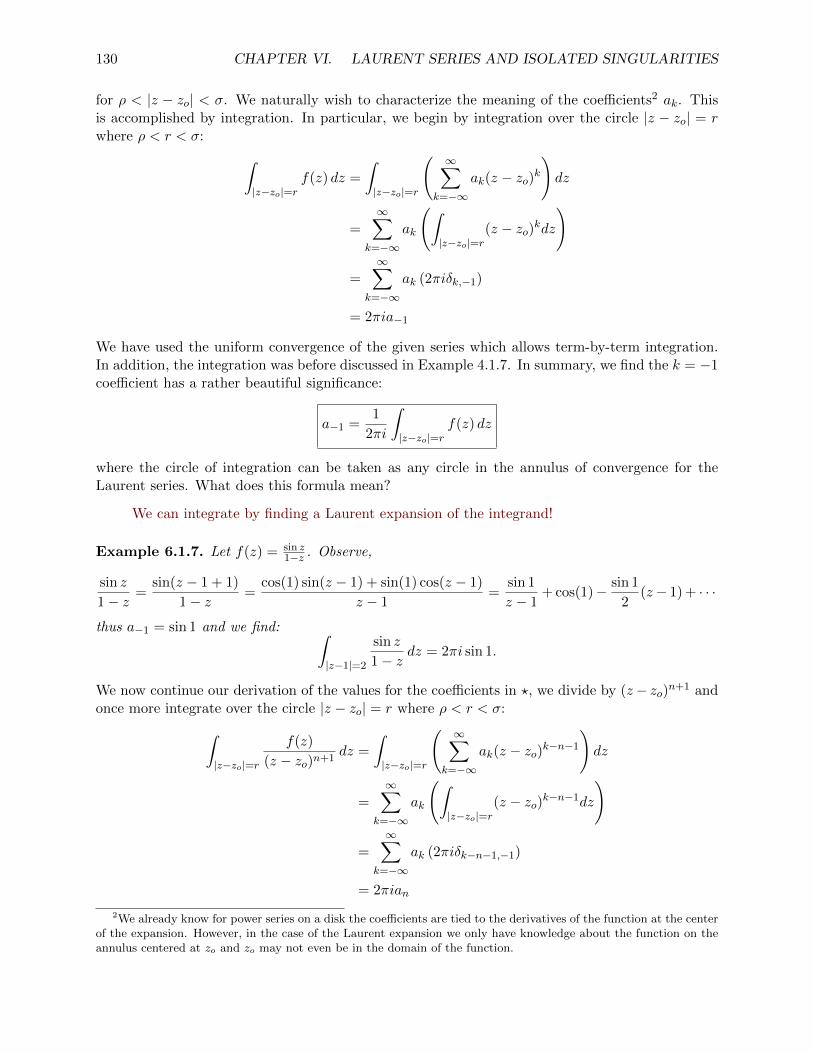
130 CHAPTER VI. LAURENT SERIES AND ISOLATED SINGULARITIES
for ρ < |z − zo| < σ. We naturally wish to characterize the meaning of the coefficients2 ak. Thisis accomplished by integration. In particular, we begin by integration over the circle |z − zo| = rwhere ρ < r < σ: ∫
|z−zo|=rf(z) dz =
∫|z−zo|=r
( ∞∑k=−∞
ak(z − zo)k)dz
=
∞∑k=−∞
ak
(∫|z−zo|=r
(z − zo)kdz
)
=
∞∑k=−∞
ak (2πiδk,−1)
= 2πia−1
We have used the uniform convergence of the given series which allows term-by-term integration.In addition, the integration was before discussed in Example 4.1.7. In summary, we find the k = −1coefficient has a rather beautiful significance:
a−1 =1
2πi
∫|z−zo|=r
f(z) dz
where the circle of integration can be taken as any circle in the annulus of convergence for theLaurent series. What does this formula mean?
We can integrate by finding a Laurent expansion of the integrand!
Example 6.1.7. Let f(z) = sin z1−z . Observe,
sin z
1− z=
sin(z − 1 + 1)
1− z=
cos(1) sin(z − 1) + sin(1) cos(z − 1)
z − 1=
sin 1
z − 1+ cos(1)− sin 1
2(z− 1) + · · ·
thus a−1 = sin 1 and we find: ∫|z−1|=2
sin z
1− zdz = 2πi sin 1.
We now continue our derivation of the values for the coefficients in ?, we divide by (z− zo)n+1 andonce more integrate over the circle |z − zo| = r where ρ < r < σ:∫
|z−zo|=r
f(z)
(z − zo)n+1dz =
∫|z−zo|=r
( ∞∑k=−∞
ak(z − zo)k−n−1
)dz
=∞∑
k=−∞ak
(∫|z−zo|=r
(z − zo)k−n−1dz
)
=∞∑
k=−∞ak (2πiδk−n−1,−1)
= 2πian
2We already know for power series on a disk the coefficients are tied to the derivatives of the function at the centerof the expansion. However, in the case of the Laurent expansion we only have knowledge about the function on theannulus centered at zo and zo may not even be in the domain of the function.

6.2. ISOLATED SINGULARITIES OF AN ANALYTIC FUNCTION 131
Once again, we have used the uniform convergence of the given series which allows term-by-term integration and the integral identity shown in Example 4.1.7. Notice the Kronecker delta
δk−n−1,−1 =
{1 if k − n− 1 = −1
0 if k − n− 1 6= −1which means the only nonzero term occurs when k−n−1 = −1
which is simply k = n. Of course, the integral is familar to us. We saw this identity for k ≥ 0 inour previous study of power series. In particular, Theorem 4.4.2 where we proved the generalizedCauchy integral formula: adapted to our current notation
1
2πi
∫|z−zo|=r
f(z)
(z − zo)n+1dz =
f (n)(zo)
n!.
For the Laurent series we study on ρ < |z − zo| < σ we cannot in general calculate f (n)(zo).However, in the case ρ = 0, we have f(z) analytic on the disk |z − zo| < σ and then we are able toeither calculate, for n ≥ 0 an by differentiation or integration. Let us collect our results for futurereference:
Theorem 6.1.8. Laurent Series Decomposition: Suppose 0 ≤ ρ < σ ≤ ∞, and suppose f(z)is analytic for ρ < |z − zo| < σ. Then f(z) can be decomposed as a Laurent series
f(z) =∞∑
n=−∞an(z − zo)n
where the coefficients an are given by:
an =1
2πi
∫|z−zo|=r
f(z)
(z − zo)n+1dz
for r > 0 with ρ < r < σ.
Notice the deformation theorem goes to show there is no hidden dependence on r in the formulationof the coefficient an. The function f is assumed holomorphic between the inner and outer circles ofthe annulus of convergence hence f(z)
(z−zo)n+1 is holomorpic on the annulus as well and the complex
integral is unchanged as we alter the value of r on (ρ, σ).
6.2 Isolated Singularities of an Analytic Function
A singularity of a function is some point which is nearly in the domain, and yet, is not. An isolatedsingularity is a singular point which is also isolated. A careful definition is given below:
Definition 6.2.1. A function f has an isolated singularity at zo if there exists r > 0 such thatf is analytic on the punctured disk 0 < |z − zo| < r.
We describe in this section how isolated singularity fall into three classes where each class hasa particular type of Laurent series about the singular point. Let me define these now and wewill explain the terms as the section continues. Notice Theorem 6.1.8 implies f(z) has a Laurentseries in a punctured disk about singularity hence the definition below covers all possible isolatedsingularities.
Definition 6.2.2. Suppose f has an isolated singularity at zo.

132 CHAPTER VI. LAURENT SERIES AND ISOLATED SINGULARITIES
(i.) If f(z) =
∞∑k=0
ak(z − zo)k then zo is a removable singularity.
(ii.) Let N ∈ N. If f(z) =∞∑
k=−Nak(z − zo)k with a−N 6= 0 then zo is a pole of order N .
(iii.) If f(z) =
∞∑k=−∞
ak(z − zo)k where ak 6= 0 for infinitely many k < 0 then zo is an essential
singularity.
We begin by studying the case of removable singularity. This is essentially the generalization of ahole in the graph you studied a few years ago.
Theorem 6.2.3. Riemann’s Theorem on Removable Singularities: let zo be an isolatedsingularity of f(z). If f(z) is bounded near zo then f(z) has a removable singularity.
Proof: expand f(z) in a Laurent series about the punctured disk at zo:
f(z) =∞∑
n=−∞an(z − zo)n
for 0 < |z − zo| < σ. If |f(z)| < M for 0 < |z − zo| < r then for r < min(σ, r) we may apply theML-theorem to the formula for the n-th coefficient of the Laurent series as given by Theorem 6.1.8
|an| =
∣∣∣∣∣ 1
2πi
∫|z−zo|=r
f(z)
(z − zo)n+1dz
∣∣∣∣∣ ≤ M(2πr)
2πrn+1=M
rn.
As r → 0 we find |an| → 0 for n < 0. Thus an = 0 for all n = −1,−2, . . . . Thus, the Laurent seriesfor f(z) reduces to a power series for f(z) on the deleted disk 0 < |z − zo| < σ and it follows wemay extend f(z) to the disk |z − zo| < σ by simply defining f(zo) = ao. �
Example 6.2.4. Let f(z) = sin zz on the punctured plane C×. Notice,
f(z) =sin z
z=
1
z
∞∑j=0
(−1)j
(2j + 1)!z2j+1 =
∞∑j=0
(−1)j
(2j + 1)!z2j = 1− 1
3!z2 + · · · .
We can extend f to C by defining f(0) = 1.
To be a bit more pedantic, f is the extension of f defined by f(z) = f(z) for z 6= 0 and f(0) = 1.The point ? The extension f is a new function which is distinct from f .
We now study poles of order N . Let us begin by making a definition:
Definition 6.2.5. Suppose f has a pole of order N at zo. If
f(z) =a−N
(z − zo)N+ · · ·+ a−1
z − zo+∞∑k=0
ak(z − zo)k
then P (z) =a−N
(z − zo)N+ · · ·+ a−1
z − zois the principal part of f(z) about zo. When N = 1 then
zo is called a simple pole, when N = 2 then zo is called a double pole.

6.2. ISOLATED SINGULARITIES OF AN ANALYTIC FUNCTION 133
Notice f(z)− P (z) is analytic.
Theorem 6.2.6. Let zo be an isolated singularity of f . Then zo is a pole of f of order N ifff(z) = g(z)/(z − zo)N where g is analytic at zo with g(zo) 6= 0.
Proof: suppose f has a pole of order N at zo then by definition it has a Laurent series whichbegins at n = −N . We calculate, for |z − zo| < r,
f(z) =
∞∑k=−N
ak(z − zo)k =1
(z − zo)N∞∑
k=−Nak(z − zo)k+N =
1
(z − zo)N∞∑j=0
aj−N (z − zo)j .
Define g(z) =∑∞
j=0 aj−N (z − zo)j and note that g is analytic at zo with g(zo) = a−N 6= 0. We
know a−N 6= 0 by the definition of a pole of order N . Thus f(z) = g(z)/(z − zo)N as claimed.
Conversely, suppose there exists g analytic at zo with g(zo) 6= 0 and f(z) = g(z)/(z − zo)N . Thereexist bo, b1, . . . with g(zo) = bo 6= 0 such that
g(z) =∞∑k=0
bk(z − zo)k
divide by (z − zo)N to obtain:
f(z) =1
(z − zo)N∞∑k=0
bk(z − zo)k =
∞∑k=0
bk(z − zo)k−N =
∞∑j=−N
bj+N (z − zo)j
identify that the coefficient of the Laurent series at order −N is precisely bo 6= 0 and thus we haveshown f has a pole of order N at zo. �
Example 6.2.7. Consider f(z) =ez
(z − 1)5. Notice ez is analytic on C hence by Theorem 6.2.6
the function f has a pole of order N = 5 at zo = 1.
Example 6.2.8. Consider f(z) =sin(z + 2)5
(z + 2)2notice
f(z) =1
(z + 2)5
((z + 2)3 − 1
3!(z + 2)9 +
1
5!(z + 2)15 + · · ·
)=
simplifying yields
f(z) =1
(z + 2)2
(1− 1
3!(z + 2)6 +
1
5!(z + 2)12 + · · ·
)︸ ︷︷ ︸
g(z)
which shows, by Theorem 6.2.6, the function f has a pole of order N = 2 at zo = −2.
Theorem 6.2.9. Let zo be an isolated singularity of f . Then zo is a pole of f of order N iff 1/fis analytic at zo with a zero of order N .

134 CHAPTER VI. LAURENT SERIES AND ISOLATED SINGULARITIES
Proof: we know f has pole of order N iff f(z) = g(z)/(z − zo)N with g(zo) 6= 0 and g ∈ O(zo).Suppose f has a pole of order N then observe
1
f(z)= (z − zo)N ·
1
g(z).
hence 1/f(z) has a zero of order N by Theorem 5.7.9. Conversely, if 1/f(z) has a zero of orderN then by Theorem 5.7.9 we have 1
f(z) = (z − zo)Nh(z) where h ∈ O(zo) and h(zo) 6= 0. Define
g(z) = 1/h(z) and note g ∈ O(zo) and g(zo) = 1/h(zo) 6= 0 moreover,
1
f(z)= (z − zo)Nh(z) ⇒ f(z) =
1
(z − zo)Nh(z)=
g(z)
(z − zo)N
and we conclude by Theorem 6.2.6 that f has a pole of order N at zo. �
The theorem above can be quite useful for quick calculation.
Example 6.2.10. f(z) = 1/ sin z has a simple pole at zo = nπ for n ∈ N ∪ {0} since
sin(z) = sin(z − nπ + nπ) = cos(nπ) sin(z − nπ) = (−1)n(z − n)π − (−1)n
3!(z − n)3 + · · ·
shows sin z has a simple zero at zo = nπ for n ∈ N ∪ {0}.
Example 6.2.11. You should be sure to study the example given by Gamelin on page 173 to 174where he derives the Laurent expansion which converges on |z| = 4 for f(z) = 1/ sin z.
Example 6.2.12. Let f(z) =1
z3(z − 2− 3i)6then f has a pole of order N = 3 at zo = 0 and a
pole of order N = 6 at z1 = 2 + 3i
Definition 6.2.13. We say a function f is meromorphic on a domain D if f is analytic on Dexcept possibly at isolated singularities of which each is a pole.
Example 6.2.14. An entire function is meromorphic on C. However, an entire function may notbe analytic at ∞. For example, sin z is not analytic at ∞ and it has an essential singularity at ∞so f(z) = sin z is not meromorphic on C ∪ {∞}.
Example 6.2.15. A rational function is formed by the quotient of two polynomials p(z), q(z) ∈ C[z]where q(z) is not identically zero; f(z) = p(z)/q(z). We will explain in Example 6.3.3 that f(z) ismeromorphic on the extended complex plane C ∪ {∞}.
Theorem 6.2.16. Let zo be an isolated singularity of f . Then zo is a pole of f of order N ≥ 1 iff|f(z)| → ∞ as z → zo.
Proof: if zo is a pole of order N then f(z) = g(z)/(z − zo)N for g(zo) 6= 0 for 0 < |z − zo| < r forsome r > 0 where g is analytic at zo. Since g is analytic at zo it is continuous and hence boundedon the disk; |g(z)| ≤M for |z − zo| < r. Thus,
|f(z)| = |g(z)(z − zo)−N | ≤M(z − zo)−N →∞
as z → zo. Thus |f(z)| → ∞ as z → zo.

6.3. ISOLATED SINGULARITY AT INFINITY 135
Conversely, suppose |f(z)| → ∞ as z → zo. Hence, there exists r > 0 such that f(z) 6= 0 for0 < |z − zo| < r. It follows that h(z) = 1/f(z) is analytic in for 0 < |z − zo| < r. Note that|f(z)| → ∞ as z → zo implies h(z) → 0 as z → zo. Thus h(z) is bounded near zo and we find byRiemann’s removable singularity Theorem 6.2.3 there exist an for n = 0, 1, 2, . . . such that:
h(z) =
∞∑n=0
an(z − zo)n
However, h(z)→ 0 as z → zo hence the extension of h(z) is zero at zo. If the zero has order N thenh(z) = (z − zo)Nb(z) where b ∈ O(zo) and b(zo) 6= 0. Therefore, we obtain f(z) = g(z)/(z − zo)Nwhere g(z) = 1/b(z) where g ∈ O(zo) and g(zo) 6= 0. We conclude zo is a pole of order N byTheorem 6.2.6.
Example 6.2.17. Let f(z) = e1z = 1+ 1
z + 12z2
+ 16z3
+ · · · . Clearly zo = 0 is an essential singularityof f . It has different behaviour than a removable singularity or a pole. First, notice for z = x > 0we have f(z) = e1/x → ∞ as x → 0+ thus f is not bounded at zo = 0. On the other hand, if we
study z = iy for y > 0 then |f(z)| = |e1iy | = 1 hence |f(z)| does not tend to ∞ along the imaginary
axis.
Theorem 6.2.18. Casorati-Weierstrauss Theorem: Let zo be an essential isolated singularityof f(z). Then for every complex number wo, there is a sequence zn → zo such that f(zn)→ wo asn→∞.
Proof: by contrapositive argument. Suppose there exists a complex number wo for which theredoes not exist a sequence zn → zo such that f(zn)→ wo as n→∞. It follows there exists ε > 0 forwhich |f(z)− wo| > ε for all z in a small punctured disk about zo. Thus, h(z) = 1/(f(z)− wo) isbounded close to zo. Consequently, zo is a removable singularity of h(z) and h(z) = (z − zo)Ng(z)for some N ≥ 0 and some analytic function g such that g(zo) 6= 0. But, this gives:
1
f(z)− wo= (z − zo)Ng(z) ⇒ f(z) = wo +
b(z)
(z − zo)N
where b = 1/g ∈ O(zo) and b(zo) 6= 0. If N = 0 then f extends to be analytic at zo. If N > 0 thenf has a pole of order N at zo. In all cases we have a contradiction to the given fact that zo is anessential singularity. The theorem follows. �
Gamelin mentions Picard’s Theorem which states that for an essential singularity at zo, for allwo except possibly one value, there is a sequence zn → zo for which f(zn) = wo for each n. In ourexample e1/z the exceptional value is wo = 0.
6.3 Isolated Singularity at Infinity
As usual, we use the reciprocal function to transfer the definition from zero to infinity.
Definition 6.3.1. We say f has an isolated singular point at ∞ if there exists r > 0 such that fis analytic on |z| > r. Equivalently, we say f has an isolated singular point at ∞ if g(w) = f(1/w)has an isolated singularity at w = 0. Furthermore, we say that the isolated singular point at ∞ isremovable singularity, a pole of order N or an essential singularity if the corresponding singularity

136 CHAPTER VI. LAURENT SERIES AND ISOLATED SINGULARITIES
at w = 0 is likewise a removable singularity, pole of order N or an essential singular point of g. Inparticular, if ∞ is a pole of order N then the Laurent series expansion:
f(z) = bNzN + · · ·+ b1z + bo +
b−1
z+b−2
z2+ · · ·
has principal part
P∞(z) = bNzN + · · ·+ b1z + bo
hence f(z)− P∞(z) is analytic at ∞.
This section is mostly a definition. I now give a few illustrative examples, partly following Gamelin.
Example 6.3.2. The function ez = 1 + z + z2/2! + z3/3! + · · · has an essential singularity at ∞.This implies that while ez is meromorphic on C, it is not meromorphic on C ∪ {∞} as it has asingularity which is not a pole or removable.
Example 6.3.3. Let p(z), q(z) ∈ C[z] with deg(p(z)) = m and deg(q(z)) = n such that m > n.Notice that long-division gives d(z), r(z) ∈ C[z] for which deg(d(z)) = m − n and deg(r(z)) < msuch that
f(z) =p(z)
q(z)= d(z) +
r(z)
q(z)
The function r(z)q(z) is analytic at ∞ and d(z) serves as the principal part. We identify f has a pole of
order m−n at ∞. It follows that any rational function is meromorphic on the extended complexplane C ∪ {∞}
Example 6.3.4. Following the last example, suppose m = n then d(z) = 0 and the singularity at∞ is seen to be removable. If p(z) = amz
m+ · · ·+ao and q(z) = bnzn+ · · ·+ bo then we can extend
f analytically at ∞ by defining f(∞) = am/bn.
Example 6.3.5. Consider f(z) = (e1/z − 1)/z for z > 0. Observe
f(z) = (e1/z − 1)/z =
(1
z+
1
2!
1
z2+
1
3!
1
z3+ · · ·
)hence the singularity at∞ is removable and we may extend f to be analytic on the extended complexplane by defining f(∞) = 0.
6.4 Partial Fractions Decomposition
In the last section we noticed in Example 6.3.3 that rational functions were meromorphic on theextended complex plane C∗ = C∪{∞}. Furthermore, it is interesting to notice the algebra of mero-morphic functions is very nice: sums, products, quotients where the denominator is not identicallyzero, all of these are once more meromorphic. In terms of abstract algebra, the set of meromorphicfunctions on a domain forms a subalgebra of the algebra of holomorphic functions on D. See pages315-320 of [R91] for a discussion which focuses on the algebraic aspects of meromorphic functions.
It turns out that not only are the rational functions meromorphic on C∗, in fact, they are the onlymeromorphic functions on C∗.
Theorem 6.4.1. A meromorphic function on C∗ is a rational function.

6.4. PARTIAL FRACTIONS DECOMPOSITION 137
Proof: let f(z) be a meromorphic function on C∗. The number of poles of f must be finiteotherwise they would acculumate to give a singularity which was not isolated. If f is analytic at∞ then we define P∞(z) = f(∞). Otherwise, f has a pole of order N and P∞(z) is a polynomialof order N . In both cases, f(z) − P∞(z) is analytic at ∞ with f(z) − P∞(z) → 0 as z → ∞. Letus label the poles in C as z1, z2, . . . , zm. Furthermore, let Pk(z) be the principal part of f(z) at zkfor k = 1, 2, . . . ,m. Notice, there exist α1, . . . , αnk such that
Pk(z) =α1
z − zk+
α2
(z − zk)2+ · · ·+ αnk
(z − zk)nk
for each k. Notice Pk(z)→ 0 as z →∞ and Pk is analytic at∞. We define (still following Gamelin)
g(z) = f(z)− P∞(z)−m∑k=1
Pk(z).
Notice g is analytic at each of the poles including ∞. Thus g is an entire function and as g(z)→ 0as z → ∞ it follows g is bounded and by Liouville’s Theorem we find g(z) = 0 for all z ∈ C.Therefore,
f(z) = P∞(z) +
m∑k=1
Pk(z).
This completes the proof as we already argued the converse direction in Example 6.3.3. �
The boxed formula is the partial fractions decomposition of f . In fact, we have shown:
Theorem 6.4.2. Every rational function has a partial fractions decomposition: in particular, ifz1, . . . , zm are the poles of f then
f(z) = P∞(z) +
m∑k=1
Pk(z)
where P∞(z) is a polynomial and Pk(z) is the principal part of f(z) around the pole zk.
The method to obtain the partial fractions decomposition of a given rational function is describedalgorithmically on pages 180-181. Essentially, the first thing to do is to we can use long-divisionto discover the principal part at ∞. Once that is done, factor the denominator to discover thepoles of f(z) and then we can simply write out a generic form of
∑mk=1 Pk(z). Then, we determine
the unknown coefficients implicit within the generic form by algebra. I will illustrate with a fewexamples:
Example 6.4.3. Let f(z) =z3 + z + 1
z2 + 1. Notice that z3 + z + 1 = z(z2 + 1) + 1 hence
f(z) = z+1
z2 + 1. We now focus on
1
z2 + 1notice z2 + 1 = (z− i)(z+ i) hence each pole is simple
and we seek complex constants A,B such that:
1
z2 + 1=
A
z + i+
B
z − i.
Multiply by z2 + 1 to obtain:1 = A(z − i) +B(z + i)

138 CHAPTER VI. LAURENT SERIES AND ISOLATED SINGULARITIES
Next, evaluate at z = −i and z = i to obtain 1 = −2iA and 1 = 2iB hence A = −1/2i andB = 1/2i and we conclude:
f(z) = z − 1
2i
1
z + i+
1
2i
1
z − i.
Example 6.4.4. Let f(z) =2z + 1
z2 − 3z − 4notice z2 − 3z − 4 = (z − 4)(z + 1) hence
2z + 1
z2 − 3z − 4=
A
z − 4+
B
z + 1⇒ 2z + 1 = A(z + 1) +B(z − 4)
Evaluate at z = −1 and z = 4 to obtain:
−1 = −5B & 9 = 5A ⇒ A = 9/5, B = 1/5.
Thus,
f(z) =1
5
(5
z − 4+
1
z + 1
)Example 6.4.5. Suppose f(z) =
1 + z
z4 − 3z3 + 3z2 − z. Long division is not needed as this is already
a proper rational function. Notice
z4 − 3z3 + 3z2 − z = z(z3 − 3z2 + 3z − 1) = z(z − 1)3.
Thus we seek: complex constants A,B,C,D for which
1 + z
z4 − 3z3 + 3z2 − z=A
z+
B
z − 1+
C
(z − 1)2+
D
(z − 1)3
Multiplying by the denominator yields,
1 + z = A(z − 1)3 +Bz(z − 1)2 + Cz(z − 1) +Dz, ?
which is nice to write as
1 + z = A(z3 − 3z2 + 3z − 1) +B(z3 − 2z2 + z) + C(z2 − z) +Dz
for what follows. Differentiating gives
1 = A(3z2 − 6z + 3) +B(3z2 − 4z + 1) + C(2z − 1) +D,d?
dz
differentiating once more yields
0 = A(6z − 6) +B(6z − 4) + C(2),d2?
dz2
differentiating for the third time:0 = 6A+ 6B
Thus A = −B. Set z = 1 in ? to obtain 2 = D. Once again, set z = 1 in d?dz to obtain 1 = C(2−1)+2
hence C = −1. Finally, set z = 1 in d2?dz2
to obtain 0 = 2B − 2 thus B = 1 and we find A = −1 asa consequence. In summary:
1 + z
z4 − 3z3 + 3z2 − z= −1
z+
1
z − 1− 1
(z − 1)2+
2
(z − 1)3.

6.4. PARTIAL FRACTIONS DECOMPOSITION 139
Perhaps you did not see the technique I used in the example above in your previous work withpartial fractions. It is a nice addition to the usual algebraic technique.
Example 6.4.6. On how partial fractions helps us find Laurent Series in the last examplewe found:
f(z) =1 + z
z4 − 3z3 + 3z2 − z= −1
z+
1
z − 1− 1
(z − 1)2+
2
(z − 1)3.
If we want the explicit Laurent series about z = 1 we simply need to expand the analytic function−1/z as a power series:
−1
z=
−1
1 + (z − 1)=∞∑n=0
(−1)n+1(z − 1)n
thus for 0 < |z − 1| < 1
f(z) =2
(z − 1)3− 1
(z − 1)2+
1
z − 1+
∞∑n=0
(−1)n+1(z − 1)n.
This is the Laurent series of f about zo = 1. The other singular point is z1 = 0. To find the Laurentseries about z1 we need to expand 1
z−1 −1
(z−1)2+ 2
(z−1)3as a power series about z1 = 0. To begin,
1
z − 1=−1
1− z= −
∞∑n=0
zn.
Let g(z) = − 1(z−1)2
and notice∫g(z)dz = C + 1
z−1 = C −∑∞
n=0 zn thus
g(z) =d
dz
[∫g(z)dz
]=
d
dz
[C −
∞∑n=0
zn
]= −
∞∑n=1
nzn−1 = −∞∑j=0
(j + 1)zj .
Let h(z) = 2/(z − 1)3 notice∫h(z)dz = −1/(z − 1)2 and
∫(∫h(z)dz)dz = 1/(z − 1) = −
∑∞n=0 z
n.I have ignored the constants of integration (why is this ok?). Observe,
h(z) =d
dz
d
dz
[∫ (∫h(z)dz
)dz
]=
d
dz
d
dz
[−∞∑n=0
zn
]=
d
dz
[−∞∑n=1
nzn−1
]
= −∞∑n=2
n(n− 1)zn−2
= −∞∑j=0
(j + 2)(j + 1)zj .
Thus, noting f(z) = −1/z + 1/(z − 1) + g(z) + h(z) we collect our calculations above to obtain:
f(z) =−1
z−∞∑j=0
(1 + (j + 1) + (j + 2)(j + 1)) zj =−1
z−∞∑j=0
(j2 + 4j + 4
)zj .
Neat, j2 + 4j + 4 = (j + 2)2 hence:
f(z) =−1
z−∞∑j=0
(j + 2)2 zj =−1
z+ 4 + 9z + 16z2 + 25z3 + 36z4 + · · · .
Term-by-term integration and differentiation allowed us to use geometric series to expand the basicrational functions which appear in the partial fractal decomposition. I hope you see the method Iused in the example above allows us a technique to go from a given partial fractal decompositionto the Laurent series about any point we wish. Of course, singular points are most fun.

140 CHAPTER VI. LAURENT SERIES AND ISOLATED SINGULARITIES

Chapter VII
The Residue Calculus
In this chapter we collect the essential tools of the residue calculus. Then, we solve a variety ofreal integrals by relating the integral of interest to the residue of a complex function. The methodwe present here is not general. Much like second semester calculus, we show some typical examplesand hold out hope the reader can generalize to similar examples. These examples date back to theearly nineteenth or late eighteenth centuries. Laplace, Poisson and ,of course, Cauchy were able touse complex analysis to solve a myriad of real integrals. That said, according to Remmert [R91]page 395:
Nevertheless there is no cannonical method of finding, for a given integrand and intervalof integration, the best path γ in C to use.
And if that isn’t sobering enough, from Ahlfors:
even complete mastery does not guarantee success
Ahlfors was a master so this comment is perhaps troubling. Generally, complex integration is anart. For example, if you peruse the answers of Ron Gordon on the Math Stackexchange Websiteyou’ll see some truly difficult problems solved by one such artist.
Some of the examples solved in this chapter are also solved by techinques of real second semestercalculus. I include such examples to illustrate the complex technique with minimal difficulty.
Keep in mind I have additional examples posted in NotesWithE100toE117. I will lecture some fromthose examples and some from these notes.
141

142 CHAPTER VII. THE RESIDUE CALCULUS
7.1 The Residue Theorem
In Theorem 6.1.8 we learned that a function with an isolated singularity has a Laurent expansion:in particular, if 0 ≤ ρ < σ ≤ ∞, and f(z) is analytic for ρ < |z − zo| < σ. Then f(z) can bedecomposed as a Laurent series
f(z) =∞∑
n=−∞an(z − zo)n
where the coefficients an are given by:
an =1
2πi
∫|z−zo|=r
f(z)
(z − zo)n+1dz
for r > 0 with ρ < r < σ. The n = −1 coefficient has special significance when we focus on theexpansion in a deleted disk about zo.
Definition 7.1.1. Suppose f(z) has an isolated singularity zo and Laurent series
f(z) =∞∑
n=−∞an(z − zo)n
for 0 < |z − zo| < ρ then we define the residue of f at zo by
Res [f(z), zo] = a−1.
Notice, the n = −1 coefficient is only the residue when we consider the deleted disk around thesingularity. Furthermore, by Theorem 6.1.8, for the Laurent series in the definition above we have
a−1 =1
2πi
∮|z−zo|=r
f(z) dz
where r is any fixed radius with 0 < r < ρ.
Example 7.1.2. Suppose n 6= 1,
Res
[1
z − zo, zo
]= 1 & Res
[1
(z − zo)n, zo
]= 0.
Example 7.1.3. In Example 6.4.3 we found
f(z) =z3 + z + 1
z2 + 1= z − 1
2i
1
z + i+
1
2i
1
z − i.
From this partial fractions decomposition we are free to read that
Res [f(z), i] =1
2i& Res [f(z),−i] =
−1
2i.
Do you understand why there is no hidden 1/(z − i) term in f(z) − 12i
1z−i? If you don’t then you
ought to read §V I.4 again.

7.1. THE RESIDUE THEOREM 143
Example 7.1.4. In Example 6.4.4 we derived:
f(z) =2z + 1
z2 − 3z − 4=
1
5
(5
z − 4+
1
z + 1
)From the above we can read:
Res [f(z), 4] = 1 & Res [f(z),−1] =1
5.
Example 7.1.5. In Example 6.4.5 we derived:
f(z) =1 + z
z4 − 3z3 + 3z2 − z= −1
z+
1
z − 1− 1
(z − 1)2+
2
(z − 1)3
By inspection of the above partial fractal decomposition we find:
Res [f(z), 0] = −1 & Res [f(z), 1] = 1.
Example 7.1.6. Consider (sin z)/z6 observe
1
z6
(z − 1
6z3 +
1
120z5 + · · ·
)=
1
z5− 1
6z3+
1
120z+ · · · .
In view of the expansion above, we find:
Res
[sin z
z6, 0
]=
1
120
Theorem 7.1.7. Cauchy’s Residue Theorem: let D be a bounded domain in the complex planewith a piecewise smooth boundary ∂D. Suppose that f is analytic on D ∪ ∂D, except for a finitenumber of isolated singularities z1, . . . , zm in D. Then∫
∂Df(z) dz = 2πi
m∑j=1
Res [f(z), zj ] .
Proof: this follows immediately from m-applications of Theorem 6.1.8. We simply parse D into msimply connected regions each of which contains just one singular point. The net-integration onlygives the boundary as the cross-cuts cancel. The picture below easily generalizes for m > 3.
Of course, we could also just envision little circles around each singularity and apply the deforma-tion theorem to reach the ∂D. �
Our focus has shifted from finding the whole Laurent series to just finding the coefficient of thereciprocal term. In the remainder of this section we examine some useful rules to find residues.

144 CHAPTER VII. THE RESIDUE CALCULUS
Proposition 7.1.8. Rule 1: if f(z) has a simple pole at zo, then
Res [f(z), zo] = limz→zo
(z − zo)f(z).
Proof: since f has a simple pole at zo we have:
f(z) =a−1
z − zo+ g(z)
where g ∈ O(zo). Hence,
limz→zo
[(z − zo)f(z)] = limz→zo
[a−1 + (z − zo)g(z)] = a−1. �
Example 7.1.9.
Res
[z3 + z + 1
z2 + 1, i
]= lim
z→i(z − i) z3 + z + 1
(z − i)(z + i)= lim
z→i
z3 + z + 1
z + i=−i+ i+ 1
i+ i=
1
2i.
You can contrast the work above with that which was required in Example 7.2.2.
Example 7.1.10. Following Example 7.1.4, let’s see how Rule 1 helps:
Res
[2z + 1
z2 − 3z − 4,−1
]= lim
z→−1(z + 1)
2z + 1
(z + 1)(z − 4)=
2(−1) + 1
−1− 4=
1
5.
Proposition 7.1.11. Rule 2: if f(z) has a double pole at zo, then
Res [f(z), zo] = limz→zo
d
dz
[(z − zo)2f(z)
].
Proof: since f has a double pole at zo we have:
f(z) =a−2
(z − zo)2+
a−1
z − zo+ g(z)
where g ∈ O(zo). Hence,
limz→zo
d
dz
[(z − zo)2f(z)
]= lim
z→zo
d
dz
[a−2 + (z − zo)a−1 + (z − zo)2g(z)
]= lim
z→zo
[a−1 + 2(z − zo)g(z) + (z − zo)2g(z)
]= a−1. �
Example 7.1.12.
Res
[1
(z3 + 1)z2, 0
]= lim
z→0
d
dz
[z2
(z3 + 1)z2
]= lim
z→0
[−3z2
(z3 + 1)2
]= 0.
Let me generalize Gamelin’s example from page 197. I replace i in Gamelin with a.
Example 7.1.13. keep in mind z2 − a2 = (z + a)(z − a),
Res
[1
(z2 − a2)2, a
]= lim
z→a
d
dz
[(z − a)2
(z2 − a2)2
]= lim
z→a
[1
(z + a)2
]=
2
(z + a)3
∣∣∣∣z=a
=−2
8a3.

7.1. THE RESIDUE THEOREM 145
In the classic text of Churchill and Brown, the rule below falls under one of the p, q theorems. See§57 of [C96]. We use the notation of Gamelin here and resist the urge to mind our p’s and q’s.
Proposition 7.1.14. Rule 3: If f, g ∈ O(zo), and if g has a simple zero at zo, then
Res
[f(z)
g(z), zo
]=f(zo)
g′(zo).
Proof: if f has a zero of order N ≥ 1 then f(z) = (z − zo)Nh(z) and g(z) = (z − zo)k(z) whereh(zo), k(zo) 6= 0 hence
f(z)
g(z)=
(z − zo)Nh(z)
(z − zo)k(z)= (z − zo)N−1h(z)
k(z)
which shows limz→zof(z)g(z) = 0 if N > 1 and for N = 1 we have limz→zo
f(z)g(z) = h(zo)
k(zo). In either case,
for N ≥ 0 we find f(z)g(z) has a removable singularity hence the residue is zero which is consistent
with the formula of the proposition as f(zo) = 0. Next, suppose f(zo) 6= 0 then by Theorem 6.2.6we have f(z)/g(z) has a simple pole hence Rule 1 applies:
Res [f(z)/g(z), zo] = limz→zo
(z − zo)f(z)
g(z)=
f(zo)
limz→zo
(g(z)−g(zo)z−zo
) =f(zo)
g′(zo).
where in the last step I used that g(zo) = 0 and g′(zo), f(zo) ∈ C with g′(zo) 6= 0 were given. �
Example 7.1.15. Observe g(z) = sin z has simple zero at zo = π since g(π) = sinπ = 0 andg′(π) = cosπ = −1 6= 0. Rule 3 hence applies as ez ∈ O(π),
Res
[ez
sin z, π
]=
eπ
cosπ= −eπ.
Example 7.1.16. Notice g(z) = (z − 3)ez has a simple zero at zo = 3. Thus, noting cos z ∈ O(3)we apply Rule 3.
Res
[cos z
(z − 3)ez, 3
]=
cos(z)
ez + (z − 3)ez
∣∣∣∣z=3
=cos(3)
e3.
One more rule to go:
Proposition 7.1.17. Rule 4: if g(z) has a simple pole at zo, then
Res
[1
g(z), zo
]=
1
g′(zo).
Proof: apply Rule 3 with f(z) = 1. �
I’ll follow Gamelin and offer this example which does clearly show why Rule 4 is so nice to know:
Example 7.1.18. note that g(z) = z2 + 1 has g(i) = 0 and g′(i) = 2i 6= 0 hence g has simple zeroat zo = i. Apply Rule 4,
Res
[1
z2 + 1, i
]=
1
2z
∣∣∣∣z=i
=1
2i.

146 CHAPTER VII. THE RESIDUE CALCULUS
7.2 Integrals Featuring Rational Functions
Let R > 0. Consider the curve ∂D which is formed by joining the line-segment [−R,R] to theupper-half of the positively oriented circle |z| = R. Let us denote the half-circle by CR hence∂D = [−R,R]∪CR. Notice the domain D is a half-disk region of radius R with the diameter alongthe real axis. If f(z) is a function which is analytic at all but a finite number of isolated singularpoints z1, . . . , zk in D then Cauchy’s Residue Theorem yields:∫
CR
f(z) dz = 2πik∑j=1
Res [f(z), zj ]
In particular, we find ∫[−R,R]
f(z) dz +
∫CR
f(z) dz = 2πik∑j=1
Res [f(z), zj ]
But, [−R,R] has z = x hence dz = dx and f(z) = f(x) for −R ≤ x ≤ R and
∫ R
−Rf(x) dx+
∫CR
f(z) dz = 2πik∑j=1
Res [f(z), zj ] .
The formula above connects integrals in the real domain to residues and the contour integral alonga half-circle CR. We can say something interesting in general for rational functions.
Suppose f(z) = p(z)q(z) where deg(q(z)) ≥ deg(p(z)) + 2. Let deg(q(z)) = n and deg(p(z)) = m
hence n − m ≥ 2. Also, assume q(x) 6= 0 for all x ∈ R so that no1 singular points fall on[−R,R]. In Problem 44 of the homework, based on an argument from page 131 of [C96], I showedthere exists R > 0 for which q(z) = anz
n + · · · + a2z2 + a1z + ao is bounded below |an|Rn/2
for |z| > R; that is |q(z)| ≥ |an|2 Rn for all |z| > R. On the other hand, it is easier to argue that
p(z) = bmzm+· · ·+b1z+bo is bounded for |z| > R by repeated application of the triangle inequality:
|p(z)| ≤ |bmzm|+ · · ·+ |b1z|+ |bo| ≤ |bm|Rm + · · ·+ |b1|R+ |bo|.
Therefore, if |z| > R as described above,
|f(z)| = |p(z)||q(z)|
≤ |bm|Rm + · · ·+ |b1|R+ |bo|
|an|2 Rn
≤ M
Rn−m
1in §V II.5 we study fractional residues which allows us to treat singularities on the boundary in a natural manner,but, for now, they are forbidden

7.2. INTEGRALS FEATURING RATIONAL FUNCTIONS 147
where M is a constant which depends on the coefficients of p(z) and q(z). Applying the ML-estimate to CR for R > 0 for which the bound applies we obtain:∣∣∣∣∫
CR
f(z) dz
∣∣∣∣ ≤ M(2πR)
Rn−m=
2Mπ
Rn−m−1
This bound applies for all R beyond some positive value hence we deduce:
limR→∞
∣∣∣∣∫CR
f(z) dz
∣∣∣∣ ≤ limR→∞
2Mπ
Rn−m−1= 0 ⇒ lim
R→∞
∫CR
f(z) dz = 0.
as n−m ≥ 2 implies n−m−1 ≥ 1. Therefore, the boxed formula provides a direct link between theso-called principal value of the real integral and the sum of the residues over the upper half-planeof C:
limR→∞
∫ R
−Rf(x) dx = 2πi
m∑j=1
Res [f(z), zj ] .
Sometimes, for explicit examples, it is expected that you show the details for the construction ofM and that you retrace the steps of the general path I sketched above. If I have no interest in thatdetail then I will tell you to use the Proposition below:
Proposition 7.2.1. If f(z) is a rational function which has no real-singularities and for which thedenominator is of degree at least two higher than the numerator then
limR→∞
∫ R
−Rf(x) dx = 2πi
k∑j=1
Res [f(z), zj ] .
where z1, . . . , zk are singular points of f(z) for which Im(zj) > 0 for j = 1, . . . , k.
Example 7.2.2. We calculate limR→∞∫ R−R
dxx2+1
by noting the complex extension of the integrand
f(z) = 1z2+1
satisfies the conditions of Proposition 7.2.1. Thus,
limR→∞
∫ R
−R
dx
x2 + 1= 2πiRes
[1
z2 + 1, i
]=
2πi
2z
∣∣∣∣z=i
=2πi
2i= π.
Thus2
∫ ∞−∞
dx
x2 + 1= π.
2so, technically, the double infinite double integral is defined by distinct parameters tending to ∞ and −∞independent of one another, however, for this integrand there is no difference between
∫ ba
dxx2+1
with a → ∞ andb→ −∞ verses a = −b = R tending to ∞. Gamelin starts to discuss this issue in §V II.6

148 CHAPTER VII. THE RESIDUE CALCULUS
You can contrast the way I did the previous example with how Gamelin presents the work.
Example 7.2.3. Consider f(z) = 1z4+1
notice singularities of this function are the fourth roots of
−1; z4 + 1 = 0 implies z ∈ (−1)1/4 = {eiπ/4, ieiπ/4,−eiπ/4,−ieiπ/4}. Only two of these fall in theupper-half plane. Thus, by Proposition 7.2.1
limR→∞
∫ R
−R
dx
x4 + 1= 2πiRes
[1
z4 + 1, eiπ/4
]+ 2πiRes
[1
z4 + 1, ieiπ/4
].
=2πi
4z3
∣∣∣∣eiπ/4
+2πi
4z3
∣∣∣∣ieiπ/4
=2πi
4ei3π/4+
2πi
4i3e3iπ/4
=π
2ei3π/4
[i+
i
i3
]=−π
2ei3π/4[1− i] =
−π2ei3π/4
√2e−iπ/4 =
π√2.
where we noted e−iπ/4/ei3π/4 = 1/eiπ = −1 to cancel the −1. It follows that:
∫ ∞−∞
dx
x4 + 1=
π√2
.
Wolfram Alpha reveals the antiderivative for the previous example can be directly calculated:∫dx
x4 + 1= (− log(x2−
√2x+1)+log(x2+
√2x+1)−2 tan−1(1−
√2x)+2 tan−1(
√2x+1))/(4
√2)+C.
Then to calculate the improper integral you just have to calculate the limit of the expression aboveat ±∞ and take the difference. That said, I think I prefer the method which is more complex.
The method used to justify Proposition 7.2.1 applies to non-rational examples as well. The keyquestion is how to bound, or more generally capture, the integral along the half-circle as R →∞.Sometimes the direct complex extension of the real integral is not wise. For example, for a > 0,when faced with ∫ ∞
−∞
p(x)
q(x)cos(ax)dx
we would not want to use f(z) = p(z) cos(az)q(z) since cos(aiy) = cosh(ay) is unbounded. Instead,
we would consider f(z) = p(z)eiaz
q(z) from which we obtain values for both∫∞−∞
p(x)q(x) cos(ax)dx and∫∞
−∞p(x)q(x) sin(ax)dx. I will not attempt to derive an analog to Proposition 7.2.1. Instead, I consider
the example presented by Gamelin.

7.3. INTEGRALS OF TRIGONOMETRIC FUNCTIONS 149
Example 7.2.4. Consider f(z) = eiaz
z2+1. Notice f has simple poles at z = ±i, the picture of
Example 7.2.2 applies here. By Rule 3,
Res
[eiaz
z2 + 1, i
]=eiaz
2z
∣∣∣∣i
=e−a
2i.
Let D be the half disk with ∂D = [−R,R] ∪ CR then by Cauchy’s Residue Theorem∫[−R,R]
eiaz
z2 + 1dz +
∫CR
eiaz
z2 + 1dz =
2πie−a
2i= πe−a ? .
For CR we have z = Reiθ for 0 ≤ θ ≤ π hence for z ∈ CR with R > 1,
|f(z)| =∣∣∣∣ eiazz2 + 1
∣∣∣∣ =1
|z2 + 1|≤ 1
||z|2 − 1|=
1
R2 − 1
Thus, by ML-estimate,∣∣∣∣∫CR
eiaz
z2 + 1dz
∣∣∣∣ ≤ 2πR
1−R2⇒ lim
R→∞
∫CR
eiaz
z2 + 1dz = 0.
Returning to ? we find:
limR→∞
∫[−R,R]
eiax
x2 + 1dx = πe−a ⇒
∫ ∞−∞
cos(ax)
x2 + 1dx+ i
∫ ∞−∞
sin(ax)
x2 + 1dx = πe−a.
The real and imaginary parts of the equation above reveal:∫ ∞−∞
cos(ax)
x2 + 1dx = πe−a &
∫ ∞−∞
sin(ax)
x2 + 1dx = 0.
In §V II.7 we learn about Jordan’s Lemma which provides an estimate which allows for integrationof expressions such as sinx
x .
7.3 Integrals of Trigonometric Functions
The idea of this section is fairly simple once you grasp it:
Given an integral involving sine or cosine find a way to represent it as the formula forthe contour integral around the unit-circle, or some appropriate curve, then use residuetheory to calculate the complex integral hence calculating the given real integral.
Let us discuss the main algebraic identities to begin: if z = eiθ = cos θ + i sin θ then z = e−iθ =cos θ− i sin θ hence cos θ = 1
2
(eiθ + e−iθ
)and sin θ = 1
2i
(eiθ − e−iθ
). Of course, we’ve known these
from earlier in the course. But, we also can see these as:
cos θ =1
2
(z +
1
z
)& sin θ =
1
2i
(z − 1
z
)moreover, dz = ieiθdθ hence dθ = dz/iz. It should be emphasized, the formulas above hold for theunit-circle.

150 CHAPTER VII. THE RESIDUE CALCULUS
Consider a complex-valued rational function R(z) with singular points z1, z2, . . . zk for which |zj | 6= 0for all j = 1, 2, . . . , k. Then, by Cauchy’s Residue Theorem∫
|z|=1R(z) dz = 2πi
∑|zj |<1
Res (R(z), zj)
In particular, as z = eiθ parametrizes |z| = 1 for 0 ≤ θ ≤ 2π,∫ 2π
0R(cos θ + i sin θ) ieiθdθ = 2πi
∑|zj |<1
Res (R(z), zj)
In examples, we often begin with∫ 2π
0 R(cos θ+i sin θ) ieiθdθ and work our way back to∫|z|=1R(z) dz.
Example 7.3.1. ∫ 2π
0
dθ
5 + 4 sin θ=
∫|z|=1
dz/iz
5− 4 · i2(z − 1
z
)=
∫|z|=1
1
i· dz
5z − 2i (z2 − 1)
=
∫|z|=1
dz
2z2 − 2 + 5iz
Notice 2z2 + 5iz− 2 = (2z+ i)(z+ 2i) = 2(z+ i/2)(z+ 2i) is zero for zo = −i/2 or z1 = −2i. Onlyzo falls inside |z| = 1 therefore, by Cauchy’s Residue Theorem,∫ 2π
0
dθ
5 + 4 sin θ=
∫|z|=1
dz
2z2 + 5iz − 2
= 2πiRes
[1
2z2 + 5iz − 2,−i/2
]= (2πi)
1
4z + 5i
∣∣∣∣z=−i/2
=2πi
−2i+ 5i
=2π
3.
The example below is approximately borrowed from Remmert page 397 [R91].
Example 7.3.2. Suppose p ∈ C with |p| 6= 1. We wish to calculate:∫ 2π
0
1
1− 2p cos θ + p2dθ.
Converting the integrand and measure to |z| = 1 yields:
1
1− p(z + 1
z
)+ p2
dz
iz=
[1
z − pz2 − p+ p2z
]dz
i=
[1
(z − p)(1− pz)
]dz
i.

7.4. INTEGRANDS WITH BRANCH POINTS 151
Hence, if |p| < 1 then z = p is in |z| ≤ 1 and it follows 1− pz 6= 0 for all points z on the unit-circle|z| = 1. Thus, we have only one singular point as we apply the Residue Theorem:∫ 2π
0
1
1− 2p cos θ + p2dθ =
∫|z|=1
[1
(z − p)(1− pz)
]dz
i= 2πRes
[1
(z − p)(1− pz), p
]By Rule 1,
Res
[1
(z − p)(1− pz), p
]= lim
z→p(z − p) 1
(z − p)(1− pz)=
1
1− p2
and we conclude: if |p| < 1 then∫ 2π
0
1
1− 2p cos θ + p2dθ =
2π
1− p2.
Suppose |p| > 1 then z − p 6= 0 for |z| = 1 and 1− pz = 0 for zo = 1/p for which |zo| = 1/|p| < 1.Thus the Residue Theorem faces just one singularity within |z| = 1 for the |p| > 1 case:∫ 2π
0
1
1− 2p cos θ + p2dθ =
∫|z|=1
[1
(z − p)(1− pz)
]dz
i= 2πRes
[1
(z − p)(1− pz), 1/p
]By Rule 1,
Res
[1
(z − p)(1− pz), 1/p
]= lim
z→1/p(z − 1/p)
1
(z − p)(z − 1/p)(−p)=
1
(1/p− p)(−p)=
1
p2 − 1,
neat. Thus, we conclude, for |p| > 1,∫ 2π
0
1
1− 2p cos θ + p2dθ =
2π
p2 − 1.
7.4 Integrands with Branch Points
Cauchy’s Residue Theorem directly applies to functions with isolated singularities. If we wish tostudy functions with branch cuts then some additional ingenuity is required. In particular, thekeyhole contour is often useful. For example, the following template could be used for branchcuts along the positive real, negative imaginary and negative real axis.

152 CHAPTER VII. THE RESIDUE CALCULUS
Example 7.4.1. Consider
∫ ∞0
xa
(1 + x)2dx where a 6= 0 and −1 < a < 1. To capture this inte-
gral we study f(z) = za
(1+z)2where za = |z|aexp(aLog0(z)) is the branch of za which has a jump-
discontinuity along θ = 0 which is also at θ = 2π. Let ΓR be the outside circle in the contourbelow. Let Γε be the small circle encircling z = 0. Furthermore, let L+ = [ε + iδ, R + iδ] andL− = [R − iδ, ε − iδ] where δ is a small positive constant3 for which δ → 0 and ε → 0. Notice, inthe limits ε→ 0 and R→∞, we have L+ → [0,∞] and L− → [∞, 0]
The singularity zo = −1 falls within the contour for R > 1 and ε < 1. By Rule 2 for residues,
Res
(za
(1 + z)2,−1
)= lim
z→−1
d
dz[za] = lim
z→−1
(aza−1
)= a(−1)a−1 = −a(eiπ)a = −aeiπa.
Cauchy’s Residue Theorem applied to the contour thus yields:∫ΓR
f(z) dz +
∫L−
f(z) dz +
∫Γε
f(z) dz +
∫L+
f(z) dz = −2πiaeiπa
If |z| = R then notice: ∣∣∣∣ za
(1 + z)2
∣∣∣∣ ≤ Ra
(R− 1)2.
Also, if |z| = ε then ∣∣∣∣ za
(1 + z)2
∣∣∣∣ ≤ εa
(1− ε)2.
In the limits ε→ 0 and R→∞ we find by the ML-estimate∣∣∣∣∫ΓR
f(z) dz
∣∣∣∣ ≤ Ra
(R− 1)2(2πR) =
2πRa−1
(1− 1/R)2→ 0
as −1 < a < 1 implies a− 1 < 0. Likewise,as a+ 1 > 0 we find:∣∣∣∣∫Γε
f(z) dz
∣∣∣∣ ≤ εa
(1− ε)2(2πε) =
2πεa+1
(1− ε)2→ 0.
We now turn to unravel the integrals along L±. For z ∈ L+ we have Arg0(z) = 0 whereas z ∈ L−we have Arg0(z) = 2π. In the limit ε→ 0 and R→∞ we have:∫
L+
za
(1 + z)2dz =
∫ ∞0
xa
(1 + x)2dx & −
∫L−
za
(1 + z)2dz =
∫ ∞0
xae2πia
(1 + x)2dx
3we choose δ as to connect L± and the inner and outer circles

7.4. INTEGRANDS WITH BRANCH POINTS 153
where the phase factor on L− arises from the definition of za by the Arg0(z) branch of the argument.Bringing it all together,∫ ∞
0
xa
(1 + x)2dx− e2πia
∫ ∞0
xa
(1 + x)2dx = −2πiaeiπa.
Solving for the integral of interest yields:∫ ∞0
xa
(1 + x)2dx =
−2πiaeiπa
1− e2πia=
πa12i (eiπa − e−iπa)
=πa
sin(πa)
At this point, Gamein remarks that the function g(w) =∫∞
0xwdx
(1+x)2is analytic on the strip
−1 < Re(w) < 1 as is the function πwsinπw thus by the identity princple we find the integral identity
holds for −1 < Re(w) < 1.
The following example appears as a homework problem on page 227 of [C96].
Example 7.4.2. Show that
∫ ∞0
dx√x(x2 + 1)
=π√2
.
Let f(z) =z−1/2
z2 + 1where the root-function has a branch cut along [0,∞]. We use the keyhole
contour introduced in the previous example. Notice z = ±i are simple poles of f(z). We considerz−1/2 = |z|−1/2exp
(−12 Log0(z)
). In other words, if z = re−θ for 0 < θ ≤ 2π then z−1/2 = 1√
reiθ/2.
Thus, for z = x in L+ we have z−1/2 = 1/√x. On the other hand for z = x in L− we have
z−1/2 = −1/√x as ei(2π)/2 = eiπ = −1. Notice, z2 + 1 = (z − i)(z + i) and apply Rule 3 to see
Res (f(z), i) =i−1/2
2i=e−iπ/4
2i& Res (f(z),−i) =
(−i)−1/2
−2i=e−3πi/4
−2i
Consequently, assuming4 the integrals along ΓR and Γε vanish as R→∞ and ε→ 0 we find:
∫ ∞0
dx√x(x2 + 1)
−∫ ∞
0
dx
−√x(x2 + 1)
= 2πi
(e−iπ/4
2i+e−3πi/4
−2i
)
Notice −1 = eiπ and eiπe−3πi/4 = eπi/4 hence:
2
∫ ∞0
dx√x(x2 + 1)
= 2π
(e−iπ/4
2+eπi/4
2
)= 2π cosπ/4 ⇒
∫ ∞0
dx√x(x2 + 1)
=π√2.
The key to success is care with the details of the branch cut. It is a critical detail. I should mentionthat E116 in the handwritten notes is worthy of study. I believe I have assigned a homeworkproblem of a similar nature. There we consider a rectangular path of integration which tends toinfinity and uncovers and interesting integral. There are also fascinating examples of wedge-shapedintegrations and many other choices I currently have not included in this set of notes.
4 I leave these details to the reader, but intuitively it is already clear the antiderivative is something like√x at
the origin and 1/√x for x→∞.

154 CHAPTER VII. THE RESIDUE CALCULUS
7.5 Fractional Residues
In general when a singularity falls on a proposed path of integration then there is no simple methodof calculation. Generically, you would make a little indentation and then take the limit as theindentation squeezes down to the point. If that limiting process uniquely produces a value thenthat gives the integral along such a path. In the case of a simple pole there is a nice reformulationof Cauchy’s Residue Theorem.
Theorem 7.5.1. If zo is a simple pole of f and Cε is an arc of |z − zo| = ε of angle α then
limε→0
∫Cε
f(z) dz = αiRes (f(z), zo) .
Proof: since f has a simple pole we have:
f(z) =A
z − zo+ g(z)
where, by the definition of residue, A = Res (f(z), zo). The arc |z−zo| = ε of angle α is parametrizedby z = zo + εeiθ for θo ≤ θ ≤ θo + α. As the arc is a bounded subset and g is analytic on the arc itfollows there exists M > 0 for which |g(z)| < M for |z − zo| = ε. Furthermore, the integral of thesingular part is calculated:∫
Cε
Adz
z − zo=
∫ θo+α
θo
Aiεeiθdθ
εeiθ= iA
∫ θo+α
θo
dθ = iαA. �
Of course this result is nicely consistent with the usual residue theorem if we consider α = 2π andthink about the deformation theorem shrinking a circular path to a point.
Example 7.5.2. Let γ = CR ∪ [−R,−1− ε]∪Cε ∪ [−1 + ε, R]. This is a half-circular path with anindentation around zo = −1. Here we assume Cε is a half-circle of radius ε above the real axis.
The aperature is π hence the fractional residue theorem yields:
limε→0
∫Cε
dz
(z + 1)(z − i)= −πiRes
(1
(z + 1)(z − i),−1
)= −πi
(1
−1− i
)=π(1 + i)
2
For |z| = R > 1 notice∣∣∣ 1
(z+1)(z−i)
∣∣∣ ≤ ∣∣∣ 1||z|−|1||·||z|−|i||
∣∣∣ = 1(R−1)2
= M . Thus, |∫CR
dz(z+1)(z−i) | ≤
πR(R−1)2
→ 0 as R→∞. Cauchy’s Residue Theorem applied to the region bounded by γ yields:∫γ
dz
(z + 1)(z − i)= 2πiRes
(1
(z + 1)(z − i),−i)
=2πi
−i+ 1= π(i− 1)
Hence, in the limit R→∞ and ε→ 0 we find:
P.V.
∫ ∞−∞
dx
(x+ 1)(x− i)+π(1 + i)
2= π(i− 1)

7.5. FRACTIONAL RESIDUES 155
Therefore,
P.V.
∫ ∞−∞
dx
(x+ 1)(x− i)=π
2(i− 3).
The quantity above is called the principle value for two reasons: first: it approaches x = ∞ andx = −∞ symmetrically, second: it approaches the improper point x = −1 from the left and right atthe same rate. The integral (which is defined in terms of asymmetric limits) itself is divergent inthis case. We define the term principal value in the next section.
Example 7.5.3. You may recall: Let γ(t) = 2√
3eit for π/2 ≤ t ≤ 3π/2. Calculate
∫γ
dz
z + 2. A
wandering math ninja stumble across your path an mutters tan(π/3) =√
3.
Residue Calculus Solution: if you imagine deforming the given arc from z = 2i√
3 to z = −2i√
3into curves which begin and end along the rays connecting z = −2 to z = ±2i
√3 then eventually
we reach tiny arcs Cε centered about z = −2 each subtending 4π/3 of arc.
Now, there must be some reason that this deformation leaves the integral unchanged since thefractional residue theorem applied to the limiting case of the small circles yields:
limε→0
∫Cε
dz
z + 2=
4π
3iRes
(1
z + 2,−2
)=
4πi
3.
Of course, direct calculation by the complex FTC yields the same:∫γ
dz
z + 2= Log0(z + 2)
∣∣∣∣−2i√
3
2i√
3
= Log0(−2i√
3 + 2)− Log0(2i√
3 + 2)
= Log0(2(1− i√
3))− Log0(2(1 + i√
3))
= ln |2(1− i√
3|+ iArg0(4 exp(5πi/3))− ln |2(1 + i√
3|+ iArg0(4 exp(πi/3))
=5πi
3− πi
3
=4πi
3
It must be that the integral along the line-segments is either zero or cancels. Notice z = −2 + t(2±2i√
3) for ε ≤ t ≤ 1 parametrizes the rays (−2,±2i√
3] in the limit ε → 0 and dz = (2 ± 2i√
3)dtthus ∫
(−2,±2i√
3]
dz
z + 2=
∫ 1
ε
dt
t= ln 1− ln ε = − ln ε.
However, the direction of the rays differs to complete the path in a consistent CCW direction. Wego from −2 to 2i
√3, but, the lower ray goes from 2i
√3 to −2. Apparently these infinities cancel
(gulp). I think the idea of this example is a dangerous game.

156 CHAPTER VII. THE RESIDUE CALCULUS
I covered the example on page 210 of Gamelin in lecture. There we derive the identity:∫ ∞0
ln(x)
x2 − 1dx =
π2
4.
by examining a half-circular path with indentations about z = 0 and z = −1.
7.6 Principal Values
If∫∞−∞ f(x) dx diverges or
∫ ba f(x)dx diverges due to a singularity for f(x) at c ∈ [a, b] then it
may still be the case that the corresponding principal values exist. When the integrals convergeabsolutely then the principal value agrees with the integral. These have mathematical applicationas Gamelin describes briefly at the conclusion of the section.
Definition 7.6.1. We define P.V.
∫ ∞−∞
f(x) dx = limR→∞
∫ R
−Rf(x) dx. Likewise, if f is continuous
on [a, c) and (c, b] then we define
P.V.
∫ b
af(x) dx = lim
ε→0+
(∫ c−ε
af(x) dx+
∫ b
c+εf(x) dx
)In retrospect, this section is out of place. We would do better to introduce the concept of principalvalue towards the beginning. For example, in [C96] this is put forth at the outset. Thus I aminspired to present the following example stolen from [C96].
Example 7.6.2. We wish to calculate∫∞
0x2
x6+1dx. The integral can be argued to exist by compar-
ison with other convergent integrals and, as the integrand is non-negative, it converges absolutely.Thus we may find P.V.
∫∞0
x2
x6+1dx to calculate
∫∞−∞
x2
x6+1dx. The integrand is even thus:∫ ∞
0
x2
x6 + 1dx =
1
2
∫ ∞−∞
x2
x6 + 1dx =
1
2P.V.
∫ ∞−∞
x2
x6 + 1dx.
Observe f(z) = z2
z6+1has singularities at solutions of z6 + 1 = 0. In particular, z ∈ (−1)1/6.
(−1)1/6 = eiπ/6{1, e2πi/6, e4πi/6,−1,−e2πi/6,−e4πi/6}= {eiπ/6, e3πi/6, e5πi/6,−eiπ/6,−e3πi/6,−e5πi/6}= {eiπ/6, i, e5πi/6,−eiπ/6,−i,−e5πi/6}
We use the half-circle path ∂D = CR ∪ [−R,R] as illustrated below:

7.7. JORDAN’S LEMMA 157
Application of Cauchy’s residue theorem requires we calculate the residue of z2
1+z6at w = eiπ/6, i
and e5πi/6. In each case we have a simple pole and Rule 3 applies:
Res
(z2
1 + z6, w
)=
w2
6w5.
Hence,
Res
(z2
1 + z6, eiπ/6
)=
(eiπ/6)2
6(eiπ/6)5=
1
6e3iπ/6=
1
6i,
and
Res
(z2
1 + z6, i
)=
(i)2
6(i)5= − 1
6i,
and
Res
(z2
1 + z6, e5iπ/6
)=
(e5iπ/6)2
6(e5iπ/6)5=
1
6e15iπ/6=
1
6i.
Therefore, ∫∂D
z2
z6 + 1dz = 2πi
(1
6i− 1
6i+
1
6i
)=π
3.
Notice if |z| = R > 1 then∣∣∣ z2
z6+1
∣∣∣ ≤ R2
R6−1hence the ML-estimate provides:
∣∣∣∣∫CR
z2
z6 + 1dz
∣∣∣∣ ≤ R2
R6 − 1(πR)→ 0
as R→∞. If z ∈ [−R,R] then z = x for −R ≤ x ≤ R and dz = dx hence∫[−R,R]
z2
z6 + 1dz =
∫ R
−R
x2
x6 + 1dx.
Thus, noting ∂D = CR ∪ [−R,R] we have:
limR→∞
∫ R
−R
x2
x6 + 1dx =
π
3⇒ P.V.
∫ ∞−∞
x2
x6 + 1dx =
π
3⇒
∫ ∞0
x2
x6 + 1dx =
π
6.
7.7 Jordan’s Lemma
Lemma 7.7.1. Jordan’s Lemma: if CR is the semi-circular contour z(θ) = Reiθ for 0 ≤ θ ≤ π,
in the upper half plane, then
∫CR
|eiz||dz| < π.
Proof: note |eiz| = exp(Re(iz)) = exp(Re(iReiθ)) = e−R sin θ and |dz| = |iReiθdθ| = Rdθ hencethe Lemma is equivalent to the claim: ∫ π
0e−R sin θ dθ <
π
R.
By definition, a concave down function has a graph that resides above its secant line. Noticey = sin θ has y′′ = − sin θ < 0 for 0 ≤ θ ≤ π/2. The secant line from (0, 0) to (π/2, 1) is y = 2θ/π.

158 CHAPTER VII. THE RESIDUE CALCULUS
Therefore, it is geometrically (and analytically) evident that sin θ ≥ 2θ/π. Consequently, followingGamelin page 216, ∫ π
0e−R sin θ dθ = 2
∫ π/2
0e−R sin θ dθ ≤ 2
∫ π/2
0e−2Rθ/π dθ
make a t = 2Rθ/π substitution to find:∫ π
0e−R sin θ dθ <
π
R
∫ 1/R
0e−tdt <
π
R
∫ ∞0
e−t dt =π
R. �
Jordan’s Lemma allows us to treat integrals of rational functions multiplied by sine or cosine wherethe rational function has a denominator function with just one higher degree than the numerator.Previously we needed two degrees higher to make the ML-estimate go through nicely. For instance,see Example 7.2.4.
Example 7.7.2. To show∫∞
0sinxx dx = π
2 we calculate the integral of f(z) = eiz
z along an indentedsemi-circular path pictured below:
Notice, for |z| = R we have:∣∣∣∣∫CR
eiz
zdz
∣∣∣∣ ≤ ∫CR
∣∣∣∣eizz∣∣∣∣ |dz| = 1
R
∫CR
∣∣eiz∣∣ |dz| < π
R
where in the last step we used Jordan’s Lemma. Thus as R→∞ we see the integral of f(z) alongCR vanishes. Suppose R → ∞ and ε → 0 then Cauchy’s residue and fractional residue theoremscombine to yield:
limR→∞
∫ R
−R
eix
xdx− πiRes
(eiz
z, 0
)+ limR→∞
∫CR
eiz
zdz = 0
hence, noting the residue is 1,
limR→∞
∫ R
−R
eix
xdx = iπ ⇒ lim
R→∞
∫ R
−R
(cosx
x+ i
sinx
x
)dx = iπ.
Note, cosxx is an odd function hence the principal value of that term vanishes. Thus,
limR→∞
i
∫ R
−R
sinx
xdx = iπ ⇒ P.V.
∫ ∞−∞
sinx
xdx = π ⇒
∫ ∞0
sinx
xdx =
π
2.

7.8. EXTERIOR DOMAINS 159
Example 7.7.3. We can calculate
∫ ∞0
x sin(2x)
x2 + 3by studying the integral of f(z) =
ze2iz
z2 + 3around
the curve γ = CR ∪ [−R,R] where CR is the half-circular path in the CCW-direction. Noticez = ±i
√3 are simple poles of f , but, only z = i
√3 falls within γ. Notice, by Rule 3,
Res
(ze2iz
z2 + 3, i√
3
)=i√
3e−2√
3
2i√
3=e−2√
3
2.
Next, we consider |z| = R, in particular notice:∣∣∣∣∫CR
ze2iz
z2 + 3dz
∣∣∣∣ ≤ ∫CR
∣∣∣∣ ze2iz
z2 + 3
∣∣∣∣ |dz| ≤ R
R2 − 3
∫CR
∣∣e2iz∣∣ |dz| ≤ R
R2 − 3
∫CR
∣∣eiz∣∣ ∣∣eiz∣∣ |dz|Notice, Jordan’s Lemma gives∫
CR
∣∣eiz∣∣ |dz| < π = π · 1
πR
∫CR
|dz| =∫CR
1
R|dz|
hence,
R
R2 − 3
∫CR
∣∣eiz∣∣ ∣∣eiz∣∣ |dz| ≤ R
R2 − 3
∫CR
∣∣eiz∣∣ 1
R|dz| = 1
R2 − 3
∫CR
∣∣eiz∣∣ |dz| < π2
R2 − 3.
Clearly as R→∞ the integral of f(z) along CR vanishes. We find the integral along [−R,R] wherez = x and dz = dx must match the product of 2πi and the residue by Cauchy’s residue theorem
limR→∞
∫ R
−R
xe2ix
x2 + 3dx = (2πi)
e−2√
3
2= πie−2
√3.
Of course, e2ix = cos(2x) + i sin(2x) and the integral of x cos(2x)x2+3
vanishes as it is an odd function.Cancelling the factor of i we derive:
limR→∞
∫ R
−R
x sin(2x)
x2 + 3dx = πe−2
√3 ⇒
∫ ∞0
x sin(2x)
x2 + 3dx =
π
2e−2√
3
We have shown the solution of Problem 4 on page 214 of [C96]. The reader will find more usefulpractice problems there as is often the case.
7.8 Exterior Domains
Exterior domains are interesting. Basically this is Cauchy’s residue theorem turned inside out.Interestingly a term appears to account for the residue at ∞. We decided to move on to the nextchapter this semester. If you are interested in further reading on this topic, you might look at: thisMSE exchange or this MSE exchange or this nice Wikipedia example or this lecture from MichaelVanValkenburgh at UC Berkeley. Enjoy.

160 CHAPTER VII. THE RESIDUE CALCULUS

Chapter VIII
The Logarithmic Integral
We just cover the basic part of Gamelin’s exposition in this chapter. It is interesting that he pro-vides a proof of the Jordan curve theorem in the smooth case. In addition, there is a nice couplepages on simply connected and equivalent conditions in view of complex analysis. All of these areinteresting, but our interests take us elsewhere this semester.
The argument principle is yet another interesting application of the residue calculus. In short,it allows us to count the number of zeros and poles of a given complex function in terms of thelogarithmic integral of the function. Then, Rouche’s Theorem provides a technique for countingzeros of a given function which has been extended by a small perturbation. Both of these sectionsgive us tools to analyze zeros of functions in surprising new ways.
8.1 The Argument Principle
Let us begin by defining the main tool for our analysis in this section:
Definition 8.1.1. Suppose f is analytic on a domain D. For a curve γ in D such that f(z) 6= 0on γ we say:
1
2πi
∫γ
f ′(z)
f(z)dz =
1
2πi
∫γd log f(z)
is the logarithmic integral of f(z) along γ.
Essentially, the logarithmic integral measures the change of log f(z) along γ.
Example 8.1.2. Consider f(z) = (z − zo)n where n ∈ Z. Let γ(z) = zo + Reiθ for 0 ≤ θ ≤ 2πk.Calculate,
f ′(z)
f(z)=n(z − zo)n−1
(z − zo)n=
n
z − zothus,
1
2πi
∫γ
f ′(z)
f(z)dz =
1
2πi
∫γ
ndz
z − zo=
n
2πi
∫ 2πk
0
Rieiθdθ
Reiθ=
n
2π
∫ 2πk
0dθ = nk.
The number k ∈ Z is the winding number of the curve and n is either (n > 0) the number ofzeros or (n < 0) −n is the number of poles inside γ. In the case n = 0 then there are neitherzeros nor poles inside γ. Our counting here is that a pole of order 5 counts as 5 poles and a zerorepeated counts as two zeros etc..
161

162 CHAPTER VIII. THE LOGARITHMIC INTEGRAL
The example above generalizes to the theorem below:
Theorem 8.1.3. argument principle I: Let D be a bounded domain with a piecewise smoothboundary ∂D, and let f be a meromorphic function on D that extends to be analytic on ∂D, suchthat f(z) 6= 0 on ∂D. Then
1
2πi
∫∂D
f ′(z)
f(z)dz = N0 −N∞,
where N0 is the number of zeros of f(z) in D and N∞ is the number of poles of f(z) in D, countingmultiplicities.
Proof: Let zo be a zero of order N for f(z) then f(z) = (z− zo)Nh(z) where h(zo) 6= 0. Calculate:
f ′(z)
f(z)=N(z − zo)N−1h(z) + (z − zo)Nh′(z)
(z − zo)Nh(z)
=N
z − zo+h′(z)
h(z)
likewise, if zo is a pole of order N then f(z) =h(z)
(z − zo)N= (z − zo)−Nh(z) hence
f ′(z)
f(z)=−N(z − zo)−N−1h(z) + (z − zo)−Nh′(z)
(z − zo)−Nh(z)
=−Nz − zo
+h′(z)
h(z)
Thus,
Res
(f ′(z)
f(z), zo
)= ±N
where (+) is for a zero of order N and (−) is for a pole of order N . Let z1, . . . , zj be the zerosand poles of f , which are finite in number as we assumed f was meromorphic. Cauchy’s residuetheorem yields:∫
∂D
f ′(z)
f(z)dz = 2πi
j∑k=1
Res
(f ′(z)
f(z), zo
)= 2πi
j∑k=1
Nk = 2πi(N0 −N∞). �
To better understand the theorem is it useful to break down the logarithmic integral. The calcu-lations below are a shorthand for the local selection of a branch of the logarithm
log(f(z)) = ln |f(z)|+ i arg(f(z)),
henced log(f(z)) = d ln |f(z)|+ id arg(f(z))
for a curve with f(z) 6= 0 along the curve it is clear that ln|f(z)| is well-defined along the curveand if z : [a, b]→ γ then ∫
γd ln |f(z)| = ln |f(b)| − ln |f(a)|.
If the curve γ is closed then f(a) = f(b) and clearly∫γd ln |f(z)| = 0.

8.1. THE ARGUMENT PRINCIPLE 163
However, the argument cannot be defined on an entire circle because we must face the 2π-jumpsomewhere. The logarithmic integral does not measure the argument of γ directly, rather, thearguments of the image of γ under f :∫
γd arg(f(z)) = arg(f(γ(b)))− arg(f(γ(a))).
For a piecewise smooth curve we simply repeat this calculation along each piece and obtain thenet-change in the argument of f as we trace out the curve.
Theorem 8.1.4. argument principle II: Let D be a bounded domain with a piecewise smoothboundary ∂D, and let f be a meromorphic function on D that extends to be analytic on ∂D, suchthat f(z) 6= 0 on ∂D. Then the increase in the argument of f(z) around the boundary of D is 2πtimes the number of zeros minus the number of poles in D,∫
∂Dd arg(f(z)) = 2π(N0 −N∞).
We have shown this is reasonable by our study of d log(f(z)) = d ln |f(z)|+ id arg(f(z)). Note,
d
dzlog(f(z)) =
f ′(z)
f(z)⇒ d log(f(z)) =
f ′(z)
f(z)dz.
Thus the Theorem 8.1.4 is a just a reformulation of Theorem 8.1.3.
Gamelin’s example on page 227-228 is fascinating. I will provide a less sophisticated example ofthe theorem above in action.
Example 8.1.5. Consider f(z) = z3 + 1. Let γ(t) = zo + Reit for R > 0 and 0 ≤ t ≤ 2π. Thus[γ] is |z − zo| = R given the positive orientation. If R = 2 and zo = 0 then
f(γ(t)) = 8e3it + 1
The points traced out by f(γ(t)) above cover a circle centered at 1 with radius 8 three times. Itfollows the argument of f(z) has increased by 6π along γ thus revealing N0 −N∞ = 3 and as f isentire we know N∞ = 0 hence N0 = 3. Of course, this is not surprising, we can solve z3 + 1 = 0to obtain z ∈ (−1)1/3. All of these zeros fall within the circle |z| = 2.
Consider R = 1 and zo = −1. Then γ(t) = −1 + eit hence
f(γ(t)) =(eit − 1
)3+ 1 = e3it − 3e2it + 3eit − 1 + 1
If we plot the path above in the complex plane we find:
Which shows f(γ(t)) increases its argument by 2π hence just one zero falls within [γ] in this case.I used Geogebra to create the image above. Notice the slider allows you to animate the path whichhelps as we study the dynamics of the argument for examples such as this. To plot, as far as Icurrently know, you’ll need to find Re(γ(t)) and Im(γ(t)) then its pretty straightforward.

164 CHAPTER VIII. THE LOGARITHMIC INTEGRAL
8.2 Rouche’s Theorem
This is certainly one of my top ten favorite theorems:
Theorem 8.2.1. Rouche’s Theorem: Let D be a bounded domain with a piecewise smoothboundary ∂D. Let f and h be analytic on D ∪ ∂D. If |h(z)| < |f(z)| for z ∈ ∂D, then f(z) andf(z) + h(z) have the same number of zeros in D, counting multiplicities.
Proof: by assumption |h(z)| < |f(z)| we cannot have a zero of f on the boundary of D hencef(z) 6= 0 for z ∈ ∂D. Moreover, it follows f(z) + h(z) 6= 0 on ∂D. Observe, for z ∈ ∂D,
f(z) + h(z) = f(z)
[1 +
h(z)
f(z)
],
We are given |h(z)| < |f(z)| thus∣∣∣h(z)f(z)
∣∣∣ < 1 and we find Re(
1 + h(z)f(z)
)> 0. Thus all the values of
1 + h(z)f(z) on ∂D fall into a half plane which permits a single-valued argument function throughout
hence any closed curve gives no gain in argument from 1 + h(z)f(z) . Moreover,
arg (f(z) + h(z)) = arg (f(z)) + arg
[1 +
h(z)
f(z)
]hence the change in arg (f(z) + h(z)) is matched by the change in arg (f(z)) and by Theorem 8.1.4,and the observation that there are no poles by assumption, we conclude the number of zeros for fand f + h are the same counting multiplicities. �
Once you understand the picture below it offers a convincing reason to believe:
The red curve we can think of as the image of f(z) for z ∈ ∂D. Note, ∂D is not pictured. Con-tinuing, the green curve is a perturbation or deformation of the red curve by the blue curve whichis the graph of h(z) for z ∈ ∂D. In order for f(z) + h(z) = 0 we need for f(z) to be cancelled byh(z). But, that is clearly impossible given the geometry.
Often the following story is offered: suppose you walk a dog on a path which is between R1 andR2 feet from a pole. If your leash is less than R1 feet then there is no way the dog can get caughton the pole. The function h(z) is like the leash, the path which doesn’t cross the origin is the redcurve and the green path is formed by the dog wandering about the path while being restricted bythe leash.

8.2. ROUCHE’S THEOREM 165
Example 8.2.2. Find the number of zeros for p(z) = z11 +12z7−3z2 +z+2 within the unit circle.Let f(z) = 12z7 and h(z) = z11− 3z2 + z+ 2 observe for |z| = 1 we have |h(z)| ≤ 1 + 3 + 1 + 2 = 7and |f(z)| = 12|z|7 = 12 hence |h(z)| ≤ f(z) for all z with |z| = 1. Observe f(z) = 12z7 has a zeroof multiplicity 7 at z = 0 hence by Rouche’s Theorem p(z) = f(z) +h(z) = z11 + 12z7− 3z2 + z+ 2also has seven zeros within the unit-circle.
Rouche’s Theorem also has great application beyond polynomial problems:
Example 8.2.3. Prove that the equation z+ 3 + 2ez = 0 has precisely one solution in the left-half-plane. The idea here is to view f(z) = z + 3 as being perturbed by h(z) = 2ez. Clearly f(−3) = 0hence if we can find a curve γ which bounds Re(z) < 0 and for which |h(γ(t))| ≤ |f(γ(t))| for allt ∈ dom(γ) then Rouche’s Theorem will provide the conclusion we desire.
Therefore, consider γ = CR ∪ [−iR, iR] where CR has z = Reit for π/2 ≤ t ≤ 3π/2.
Consider z ∈ [−iR, iR] then z = iy for −R ≤ y ≤ R observe:
|f(z)| = |iy + 3| =√
9 + y2 & |h(z)| = |2eiy| = 2
thus |h(z)| < |f(z)| for all z ∈ [−iR, iR]. Next, suppose z = x + iy ∈ CR hence −R ≤ x ≤ 0 and−R ≤ y ≤ R with x2 + y2 = R2. In particular, assume R > 5. Note:
|f(z)| = |x+ iy + 3| ⇒ R− 3 ≤ |f(z)| ≤√
9 +R2.
the claim above is easy to see geometrically as |z + 3| is simply the distance from z to −3 whichis smallest when y = 0 and largest when x = 0. Furthermore, as −R ≤ x ≤ 0 and ex is a strictlyincreasing function,
|h(z)| =∣∣2exeiy∣∣ = 2ex < 2 < R− 3 < |f(z)|
where you now hopefully appreciate why we assumed R > 5. Consequently |h(z)| ≤ |f(z)| for allz ∈ CR with R > 5. We find by Rouche’s Theorem f(z) and f(z) +h(z) = z+ 3 + 2ez has only onezero in γ for R > 5. Thus, suppose R → ∞ and observe γ serves as the boundary of Re(z) < 0and so the equation z + 3 + 2ez = 0 has just one solution in the left-half plane.
Notice, Rouche’s Theorem does not tell us what the solution of z + 3 + 2ez = 0 with Re(z) < 0 is.The theorem merely tells us that the solution uniquely exists.
Example 8.2.4. Consider p(z) = anzn+an−1z
n−1 + · · ·+a1z+ao where an 6= 0. Let f(z) = anzn
and h(z) = an−1zn−1 + · · · + a1z + ao then p(z) = f(z) + h(z). Moreover, if we choose R > 0
sufficiently large then |h(z)| ≤ |an−1|Rn−1 + · · ·+ |a1|R + |ao| < |an|Rn = |f(z)| for |z| = R henceRouche’s Theorem tells us that there are n-zeros for p(z) inside |z| = R as it is clear that z = 0 isa zero of multiplicity n for f(z) = anz
n. Thus every p(z) ∈ C[z] has n-zeros, counting multiplicity,on the complex plane.
The proof of the Fundamental Theorem of Algebra above is nicely direct in contrast to other proofsby contradiction we saw in previous parts of this course.

166 CHAPTER VIII. THE LOGARITHMIC INTEGRAL

Chapter XIII
Approximation Theorems
I change posture in this chapter. In previous chapters I have generally made a serious effort toreplicate theorems and augment or at least duplicate proofs offered by Gamelin. In contrast, inthis chapter I will state some theorems without proof. My goal here is more akin to the typicalcalculus course at most universities or differential equations as I teach it here; I state theoremsand support your understanding with examples. Many of the deep theorems here are existencetheorems and the proofs are not that hard to understand, if you wish to discuss any of the proofsin office hours I’m happy to accommodate. That said, our goal in this chapter is come to somesemi-formal understanding of infinite products and the result of Mittag-Leffler. I defer to Gamelinfor proof that the given examples are uniformly convergent on the domain of consideration. Again,I will claim a few things in this chapter that I leave the proof to Gamelin.
I’m also going to bring in some deep results from other texts. Yet again we will see that the residuecalculus gives us insight it seems we ought not have from our minimal effort here.
13.1 Runge’s Theorem
This section would be very important if I was serious about working through all the proofs in thischapter. However, we will content ourselves with the statement of Runge’s Theorem. Notice theterminology approximated uniformly by rational functions means that there is a sequence of rationalfunctions which converges uniformly to the given function.
Theorem 13.1.1. Runge’s Theorem: Let K be a compact subset of C. If f(z) is analytic on anopen set containing K, then f(z) can be approximated uniformly on K by rational functions withpoles off K.
Proof: see pages 342-343 in Gamelin. It’s not that hard really, our focus is just elsewhere. �
Theorem 13.1.2. Let K be a compact subset of C and let U be a connected open set in C∗ whichis disjoint from K. Also, let zo ∈ U . Every rational function with poles in U can be uniformlyapproximated on K by rational functions with poles at zo
Proof: see page 343-344. It involves translating the poles, a connected argument and of course thegeometric series. This would take some time to digest. �
There are additional comments in Gamelin which are not terribly relevant to our purposes here.
167

168 CHAPTER XIII. APPROXIMATION THEOREMS
13.2 The Mittag-Leffler Theorem
I used to think Mittag-Leffler was a pair of authors, however, that is incorrect. His full name wasMagnus Gustaf Mittag-Leffler. There is no Nobel Prize in Mathematics. A popular rumor blaimsMittag-Leffler for this anomaly. The rumor would seem to be wrong, but, perhaps the general ideathat Mittag-Leffler has something to do with the lack of a math Nobel Prize seems to have someevidence. I found the article at Fields Institute helpful. I should mention, the Fields Medal isgiven to young research mathematicians whose work is important to the international communityof Mathematics.
Theorem 13.2.1. Let D be a domain in C. Let {zk} be a sequence of distinct points in D withno accumulation point in D, and let Pk(z) be a polynomial in 1
z−zk . Then, there is a meromorphicfunction f(z) on D whose poles are the points zk, such that f(z)− Pk(z) is analytic at zk.
Proof: see page 348 of Gamelin. �
Example 13.2.2. We wish to find a meromorphic function on C whose only poles are simple poles
at k ∈ N. Naturally, we consider Pk(z) =1
z − kfor the principal parts. We can try the naive guess
of fnaive(z) =∞∑k=1
1
z − k. However,
fnaive(0) = −∞∑k=1
1
k= −∞
So, to fix this, we add the p = 1 series:
f(z) =∞∑k=1
[1
z − k+
1
k
].
Now, we find f(0) = 0 and it can be verified that this series of functions converges uniformly onC − N. Moreover, it has simple poles at each k ∈ N. See page 348-349 for some detail about theuniform convergence.
Example 13.2.3. Suppose ω1, ω2 are two complex numbers which are no colinear. The lattice ofpoints L = ω1Z+ω2Z gives a discrete set of isolated points in C. We can construct a meromorphicfunction which has a double-pole at each lattice point as follows:
P(z) =1
z2+
∑(m,n)6=(0,0)
[1
(z −mω1 − nω2)2− 1
(mω1 + nω2)2
].
As in our first example, the terms − 1(mω1+nω2)2
is added to remove the infinity implicit within the
naive guess∑ 1
(z−mω1−nω2)2. This is a well-known example, the function P is the Weierstrauss
P-function. It is meromorphic on C and is doubly periodic with periods ω1, ω2 meaning
P(z + ω1) = P(z) & P(z + ω2) = P(z)
for all z ∈ dom(P) = C− L.

13.2. THE MITTAG-LEFFLER THEOREM 169
Example 13.2.4. The following identity is an example of Mittag-Leffler’s Theorem in action:
π2
sin2(πz)=
∞∑k=−∞
1
(z − k)2.
To verify the validity of this identity, set f(z) =π2
sin2(πz)and g(z) =
∞∑k=−∞
1
(z − k)2. Both f(z)
and g(z) have double-poles with matching principle parts at each k ∈ Z. We can see f(z) − g(z)is entire. Gamelin then argues that f(z) − g(z) is bounded and as f(z), g(z) → 0 as |y| → ∞ we
have f(z)− g(z) = 0 for all z ∈ C hence the claim is true. We sayπ2
sin2(πz)=
∞∑k=−∞
1
(z − k)2is a
partial fractions decomposition of π2
sin2(πz).
This is an extension of the concept of partial fractions. In our previous work, in §6.4 there werefinitely many basic rational functions whose sum captured the rational function. Notice the function
π2
sin2(πz)has an essential singularity at∞ hence it is not meromorphic on the extended complex plane
C∗. If we just have a function which is meromorphic on C then the partial fractions decompositionmay require infinitely many terms to capture the possibly infinite number of poles for the givenfunction.
Example 13.2.5. The series∑∞
k=−∞1
(z−k)2is shown to converge uniformly in Gamelin. Therefore,
we are able to perform term-by-term calculus as we discussed in Theorem 5.2.9. Notice,∫π2
sin2(πz)dz =
∫π2 csc2(πz) dz = −π cot(πz).
on the other hand, ∫ ∞∑k=−∞
1
(z − k)2dz =
∞∑k=−∞
−1
z − k
= −0∑
k=−∞
1
z − k− 1
z−∞∑k=0
1
z − k
= −1
z−∞∑j=0
1
z + j−∞∑k=0
1
z − k
= −1
z−∞∑k=0
[1
z + k+
1
z − k
]
= −1
z− 2z
∞∑k=0
1
z2 − k2.
Hence we derive:
π cot(πz) =1
z+ 2z
∞∑k=0
1
z2 − k2.

170 CHAPTER XIII. APPROXIMATION THEOREMS
13.3 Infinite Products
An infinite product is formed by multiplying arbitrarily many factors. If finitely many factors arezero then the product converges to zero. However, if infinitely many factors are zero then we saythe product diverges. In part, this is due to the role we allow the logarithm to play in what follows:
Definition 13.3.1. Let pj ∈ C for j ∈ N. If finitely many pj = 0 then we define∞∏j=1
pj = 0.
However, if pj 6= 0 for all j ∈ N then∞∏j=1
pj converges if pj → 1 and∑∞
j=1 Log(pj) converges.
Moreover, in the case∞∏j=1
pj = 0 converges,
∞∏j=1
pj = exp
∞∑j=1
Log(pj)
.
In the convergent case, we are also free to express the product as the limit of partial products:
∞∏j=1
pj = limn→∞
n∏j=1
pj .
The definition given above is partly of convenience. If you wish to read a more leisurely accountyou might see [RR91] Section 1 of Chapter 1. Another good source is Chapter 7 of [M99]. I alsoenjoy Section 3.6 of [A03]. We will find additional insights from these sources.
Example 13.3.2. If p42 = 0 and pj = 1 for all j 6= 42 then
∞∏j=1
pj = 0.
Example 13.3.3. If pj = 1 − 1j2
for all j ≥ 2 then you can directly calculate the partial productswith some effort. For example, when n = 4 we calculate,(
1− 1
4
)(1− 1
9
)(1− 1
16
)=
3
4
8
9
15
16=
5
8=
1
2
(1 +
1
4
).
Indeed, if you calculate further products you’ll see the above is the general pattern and you canargue by induction that:
n∏j=2
(1− 1
j2
)=
1
2
(1 +
1
n
).
Therefore,∞∏j=2
(1− 1
j2
)= lim
n→∞
1
2
(1 +
1
n
)=
1
2.
Example 13.3.4. The product
∞∏j=2
(1− 1
j
)is divergent despite the fact 1−1
j → 1 since∑∞
j=2 Log(
1− 1j
)diverges to −∞. Formally, the product diverges to zero since exp(−∞) = 0.

13.3. INFINITE PRODUCTS 171
Example 13.3.5. Consider the infinite product formed by pk = 1 + (−1)k+1
k for k ≥ 1,
∞∏k=1
(1 +
(−1)k+1
k
)=
(1 +
1
1
)(1− 1
2
)(1 +
1
3
)(1− 1
4
)· · ·
= limk→∞
[2 · 1
2· 4
3· 3
4· · ·(
1 +(−1)k+1
k
)· · ·]
The pattern is apparent:∏2nk=1
(1 + (−1)k+1
k
)= 1 whereas
∏2n+1k=1
(1 + (−1)k+1
k
)=(
1 + (−1)n+1
n
).
We see the partial product tend to 1 as n→∞ hence
∞∏k=1
(1 +
(−1)k+1
k
)= 1.
It is interesting to compare the previous pair of examples. Just as with series, the introduction ofsome signs can make a giant difference in the nature of the problem. There are also convergencecriteria known for products. To begin, we shift terminology a bit. Introduce aj for which pj = 1+aj .In this nomenclature we need:
(i.) only finitely many aj = −1
(ii.) aj → 0 as j →∞.
Furthermore,
Theorem 13.3.6. If aj ≥ 0 then∏
(1 + aj) converges iff∑aj converges.
Proof: see page 353 of Gamelin. �
Example 13.3.7.∞∏k=1
(1 +
1
kα
)=
{converges if α > 1
diverges if α ≤ 1.
The definition of absolute convergence is perhaps a bit surprising: look ahead to Example 13.3.11for why the naive definition fails.
Definition 13.3.8. The product∏
(1 + ak) is said to converge absolutely if ak → 0 and∑Log(1 + ak) converges absolutely, where we sum over the terms with ak 6= −1.
Notice absolute convergence of∑
Log(1 + ak) implies convergence of∑
Log(1 + ak) hence, asak → 0, we see absolute convergence of a product implies convergence of a product. In fact, asargued by Gamelin on pg. 354,
Theorem 13.3.9. The infinite product∏
(1+aj) converges absolutely if and only if∑aj converges
absolutely. This occurs if and only if∏
(1 + |aj |) converges.
Example 13.3.10. We argued in Example 13.3.5 that∞∏k=1
(1 +
(−1)k+1
k
)= 1. However, we also
saw in the α = 1 case of Example 13.3.7 that
∞∏k=1
(1 +
1
k
)diverged. We see that convergence need
not imply absolute convergence for products.

172 CHAPTER XIII. APPROXIMATION THEOREMS
Example 13.3.11. The product
∞∏k=1
(1 +
i
k
)does not converge since Log(1+i/k) = i/k+O(1/k2).
Notice∑i/k diverges thus Log(1 + i/k) also diverges. On the other hand, following Gamelin,
Log
∣∣∣∣1 +i
k
∣∣∣∣ = Log
√1 +
1
k2=
1
2Log
(1 +
1
k2
)< 1/k2
Thus∑
Log∣∣1 + i
k
∣∣ converges by comparison to p = 2 series. Hence
∞∏k=1
∣∣∣∣1 +i
k
∣∣∣∣ converges.
The Weierstrauss M -test for products of functions is given below:
Theorem 13.3.12. Suppose that gk(z) = 1 +hk(z), k ≥ 1, are functions on a set E ⊆ C. Supposethere are constants Mk > 0 such that
∑Mk <∞, and |h(z)| ≤Mk for all z ∈ E. Then
∏mk=1 gk(z)
converges uniformly to∏∞k=1 gk(z) on E as m→∞.
Proof: see page 354-355 of Gamelin. Or, see pages 160-161 of [A03]. �
It should be noted that uniform convergence on compact subsets of a given domain is known asnormal convergence for the product. As before, the Weierstrauss test does give us normal con-vergence of a product. Notice Gamelin uses the terminology normal convergence in the Theoremon logarthmic differentiation.
If G(z) = g1(z)g2(z) · · · gm(z) then m-fold product rule and some easy algebra reveal:
G′(z)
G(z)=g′1(z)
g1(z)+g′2(z)
g2(z)+ · · ·+ g′m(z)
gm(z).
The expression above is the logarithmic derivative of G as d [logG(z)] = G′(z)G(z) dz. If we have a
uniformly convergent infinite product then the technique of logarthmic differentiation has a naturalextension:
Theorem 13.3.13. Let gk(z), k ≥ 1, be analytic functions on a domain D such that the product∏mk=1 gk(z) converges normally on D to G(z) =
∏∞k=1 gk(z). Then
G′(z)
G(z)=∞∑k=1
g′k(z)
gk(z)
where the sum converges normally on D.
Proof: fairly routine combination of other results. See page 355 Gamelin. Alternatively, see pages167-169 of [A03] where Mittag-Leffler and the logarithmic differentation are discussed. �
13.4 The Weierstrauss Product Theorem
Theorem 13.4.1. Weierstrauss Product Theorem: Let D be a domain in the complex plane.Let {zk} be a sequence of distinct points with no accumulation point in D, and let {nk} be a sequenceof integers (positive or negative). Then there is a meromorphic function f(z) on D whose only zerosand poles are the points zk such that the order of f(z) at zk is nk (negative order is pole of order−nk, zero order is removable singularity, postive order is a zero of order nk)

13.4. THE WEIERSTRAUSS PRODUCT THEOREM 173
Proof: proof is found on page 358-359. I am tempted to cover it as the method of the proofis similar to the thought process for constructing the examples I’ve seen in the text books thusfar. We write down the naive product which produces the required poles and zeros, then, as thatdiverges, we multiply by a suitable convergence factor. �
Some intuition for the form of the convergence factors is given by the simple argument here: supposeF (z), G(z) are entire functions on C which share the same zeros with matching multiplicities. ThenFG is naturally1 identified with an entire function which has no zeros. Thus h(z) = log(F (z)/G(z))
is defined for all z ∈ C and h(z) is an entire function. Consequently, F (z) = eh(z)G(z) for all z ∈ C.
The example below is interesting in that no convergence factor is required.
Example 13.4.2. Consider
∞∏k=1
(1− z2
k2
). In the terminology of Theorem 13.3.12 we have gk(z) =
1− z2
k2and hk(z) = −z2
k2. Suppose |z| ≤ R then
∣∣∣ z2k2 ∣∣∣ ≤ R2
k2. Observe,
∑∞k=1
R2
k2= πR2
6 hence Theorem
13.3.12 applies and we find the product is uniformly convergent for |z| < R. But, as R is arbitrary
we find the productm∏k=1
(1− z2
k2
)converges uniformly to
∞∏k=1
(1− z2
k2
)on C.
I found the inequality arguments in the example below on page 162-163 of [A03].
Example 13.4.3. Consider∞∏k=1
(1 +
z
k
)e−z/k. Observe,
log [(1− w)ew] = log(1− w) + w = −w − w2
2− w3
3− w4
4− · · ·+ w = −w
2
2− w3
3− w4
4− · · · .
Hence, if |w| < 1/2 then
|log [(1− w)ew]| ≤ |w|2(
1
2+
1
22+
1
23+ · · ·
)=
(1/2)|w|2
1− 1/2= |w|2.
Identify w = z/k and consider |z| < R and k > 2R. We find:∣∣∣log[(
1− z
k
)ezk
]∣∣∣ ≤ ∣∣∣∣z2
k2
∣∣∣∣ ≤ R2
k2.
Fix ko > 2R and note
∞∏k=1
(1 +
z
k
)e−z/k =
ko−1∏k=1
(1 +
z
k
)e−z/k
∞∏k=ko
(1 +
z
k
)e−z/k.
Observe the infinite product in the expression above converges uniformly by the Weierstrauss M -test
as∑∞
k=koR2
k2≤∑∞
k=1R2
k2= πR2
6 thus
∞∏k=1
(1 +
z
k
)e−z/k converges uniformly on a disk of abritrary
radius hence
∞∏k=1
(1 +
z
k
)e−z/k converges uniformly on C.
1the singularities of this function are removable by the fact that the zeros of F and G match

174 CHAPTER XIII. APPROXIMATION THEOREMS
It is interesting to note the ubiquity of the example which follows below: see page 355 of Gamelin,or page 169 of [A03], or for a slightly different take [M99] see Example 7.1.10 of page 424. Thisexample shows how Mittag-Leffler series can connect to the infinite products.
Example 13.4.4. Consider G(z) = sin(πz) and F (z) = z∞∏k=1
(1− z2
k2
). We know F (z) is entire
by our study in Example 13.4.2. Furthermore, we observe both G(z) and F (z) share simple zerosat z = k ∈ Z. Therefore, there exists h(z) for which G(z) = eh(z)F (z). We can derive the factoreh(z) by the logarithmic differentiation argument which follows: consider, by Theorem 13.3.13
d
dzlog(F (z)) =
F ′(z)
F (z)=
1
z+∞∑k=1
−2z/k2
1− z2/k2=
1
z+∞∑k=1
2z
z2 − k2= π cotπz,
where you may recall we derived the infinite series for the cotangent function in Example 13.2.5.Next, integrate the expression above, note the uniform convergence allows us term-by-term calculuson the series hence:
log(sin(πz)) = C1 + log(z) +∞∑k=1
log(z2 − k2) = C2 + log(z) +∞∑k=1
log(1− z2/k2)
Thus, by the definition of the infinite product,
sin(πz) = zeC2
∞∏k=1
(1− z2
k2
).
Finally, observe sin(πz)z → π as z → 0 hence in the limit z → 0 we find:
sin(πz)
z= eC2
∞∏k=1
(1− z2
k2
)→ eC2 = π.
We conclude,
sin(πz) = πz∞∏k=1
(1− z2
k2
).
In retrospect, eh(z) = π.
Finally, I leave you with an interesting theorem I found in [RR91] page 11:
Theorem 13.4.5. multiplicative analogue of Taylor series: If f is holomorphic at the origin,then f can be represented uniquely in a disc B about 0 as a product
f(z) = bzN∞∏k=1
(1 + bkzk),
where b, bk ∈ C and N ∈ N, which converges normally in B to f .
This theorem was shown by J.F. Ritt in 1929. Notice the disc on which the product represents fneed not be as large as the disc on which f is holomorphic.
Remark: I plan to cover some connections between residue calculus and series calculations. Iintend to follow this short introductory article Infinite Series and the Residue Theorem by NoahHughes who was a student at Appalachian State University who I met due to his studies with mybrother.

Chapter XIV
Some Special Functions
In lecture I worked through the calculations in the first section of this chapter. I did not addanything of significance so I will not type those notes. However, a pdf of my handwritten calculationsis posted at my website in the complex analysis page. I did not have much to say about the middlesections in this chapter. Finally, for the final section I used the excellent lecture by Ethan Smithfrom 2013 which adds considerable insight to the discussion of the Prime Number Theorem.
14.1 The Gamma Function
14.2 Laplace Transforms
14.3 The Zeta Function
14.4 Dirichlet Series
14.5 The Prime Number Theorem
References
[A03] M.J. Ablowitz and A.S. Fokas, “Complex Variables Introduction and Applica-tions,” Cambridge, second ed. 2003.
[C96] R.V. Churchill and J.W. Brown, “Complex Variables and Applications,” McGrawHill, sixth ed. 1996.
[E91] E. Ebbinghaus et. al., “Numbers,” Springer Verlag, 1991, volume 123.
[A03] E. Freitag and R. Busam, “Complex Analysis,” Springer, second ed. 2009.
[J02] R. Johnsonbaugh and W.E. Pfaffenberger, “Foundations of Mathematical Anal-ysis,” Dover, 2002.
[M99] J.E. Marsden and M.J. Hoffman, “Basic Complex Analysis,” W.H. Freeman andCompany, third ed. 1999.
[R91] R. Remmert, “Theory of Complex Functions,” Springer Verlag, 1991, volume 122.
175

176 CHAPTER XIV. SOME SPECIAL FUNCTIONS
[RR91] R. Remmert, “Classical Topics in Complex Function Theory,” Springer Verlag, 1991,volume 172.
[R76] W. Rudin, “Principles of Mathematical Analysis (International Series in Pure andApplied Mathematics),” McGraw Hill, 1976.


![Complex Analysis[gamelin.pdf]](https://img.dokumen.tips/doc/110x75/55cf9cbc550346d033aadb5d/complex-analysisgamelinpdf.jpg)