GUIDE An optimization approach to multiprobe cryosurgery ...mida.dima.unige.it/files/cryo.pdf · September 26, 2011 14:19 Computer Methods in Biomechanics and Biomedical Engineering

September 26, 2011 14:19 Computer Methods in Biomechanics and Biomedical Engineering ms-2011-07-07

Computer Methods in Biomechanics and Biomedical EngineeringVol. 00, No. 00, May 2008, 1–14

GUIDE

An optimization approach to multiprobe cryosurgery planning

Giovanni Giorgia, Leopoldo Avallea, Massimo Brignoneb, Michele Pianaa,c∗ and Giacomo

Cavigliaa

aDipartimento di Matematica, Universita di Genova; bAzienda Ospedaliera Universitaria

San Martino, Genova; cConsiglio Nazionale delle Ricerche CNR - SPIN, Genova(Received 00 Month 200x; final version received 00 Month 200x)

In cryosurgery operations tumoral cells are killed by means of a freezing procedure realizedwith insertion of cryoprobes in the diseased tissue. Cryosurgery planning aims at establishingthe best values for operation parameters like number and position of the probes or temperatureand duration of the freezing process. Here we present an application of Ant ColonyOptimization (ACO) to cryosurgery planning, whereby the ACO cost functionis computed by numerically solving several direct Stefan problems for biologicaltissues. The method is validated in the case of a 2D phantom of a prostate cross-section.

Keywords: Cryosurgery planning, Euler-Galerkin method, Ant Colony Optimization.

1. Introduction

Cryosurgery is a minimally invasive technique aiming at thedestruction of cancerous tissues by application of extremelycold temperatures. It may be used in the treatment of localizedprostate and liver carcinomas, in alternative to resection, radiation andchemotherapy (Cohen 2004; Theodorescu 2004; Zhang et al 2005;Chua and Chou 2009; Shitzer 2011).The cooling and the subsequent destruction of living tissues is performed by

insertion of multiple cryoprobes in the shape of long hypodermic needles connectedto an external generator of supercooled fluid (Rossi et al 2010). Subtraction of heatfrom the biological system leads to a phase change from the liquid to the solidstate, starting around the tip of the cryprobes. The process is carried on until theentire cancerous tissue is frozen with temperature range of the solid phase belowthe lethal limit. To obtain an effective destruction of cancerous tissues severalfreezing-thawing cycles at appropriate temperature variation rates may be required(Chua and Chou 2009). To minimize cryoinjury to the surrounding healthy cellsand blood vessels, cryoheaters have also been developed, to be inserted into thetissues (Rabin and Stahovich 2003; Rossi et al 2010).A reliable mathematical model of cryosurgery operation requires the determina-

tion of the spatial distribution and time evolution of the temperature field insidethe tissue volume, when heat is subtracted by the cryoprobes and new heat en-ters the unfrozen subregions of the tissue, as a consequence of blood perfusion andmetabolism. Cryoprobes, cryoheaters and healthy tissue around the tumor provide

∗Corresponding author. Email:[email protected]

ISSN: 1741-5977 print/ISSN 1741-5985 onlinec⃝ 2008 Taylor & FrancisDOI: 10.1080/1741597YYxxxxxxxxhttp://www.informaworld.com


2 Taylor & Francis and I.T. Consultant

boundary data for the temperature transient field. Thus the determination of thetransient temperature reduces to the solution of a (direct) Stefan problem for aphase change.Unlike pure substances, biological tissues do not have a fixed freezing point but

phase changes are taken to occur over a temperature range, so that between thesolid phase and the normal tissue there is an intermediate, time dependent spa-tial region (Shitzer 2011; Chua and Chou 2009; Rabin and Shitzer 1998). A furthercomplication arises from the fact that analytic solutions of the propagation equa-tion are seldom at disposal and therefore only numerical methods can provide anadequate framework for cryosurgery simulations.In order to destroy cancerous tissues while preserving the ad-

jacent healthy organs, the design of a cryosurgery operationrequires the optimal choice of placements of cryoprobes withthe related shapes and dimensions (Keanini and Rubinsky 1992;Rabin and Stahovich 2003; Rabin et al 2004), the most appropriate in-sertion depth (Rossi et al 2007), the optimal temperature law for thecryoprobes (Baissalov et al 2000). Among the optimization techniques em-ployed we recall the simplex method (Keanini and Rubinsky 1992), the gradient-descent method (Baissalov et al 2001), the force-field analogy (Rossi et al 2010;Tanaka et al 2006), the bubble-packing method (Rossi et al 2008).In this paper we describe a new systematic procedure to deal with

cryosurgery planning based on the application of the Ant Colony Opti-mization (ACO) method (Socha and Dorigo 2003). The novelty of thisapproach lies in the generality of its formulation since ACO is inde-pendent from the physical interpretation and from the number of theparameters subjected to optimization. In other words, trough ACO, oneis able to set different kinds of free planning parameters without chang-ing the optimization technique.As a first application, here we consider the problem of determining the best

location for cryprobes and cryoheaters. The algorithm is based on an itera-tive procedure consisting in the solution of several (direct) Stefan prob-lems at each step. Every step begins with the assumption that the placementof cryoprobes and cryoheaters is given while cryoprobes, cryoheaters, tumor andbackground tissue are at the temperature of 37 oC. Next the direct Stefan prob-lem is solved as the temperature of the cryoprobes is lowered down to −145 oC,until the tumor is almost completely frozen. The resulting temperature field is pro-cessed to evaluate the defect weight function (Lung et al 2004) providing aquantitative estimate of the mismatch between the frozen tissue at sufficiently lowtemperature and the tissue to be destroyed. ACO utilizes this cost functionaland yields the new positions of cryoprobes and cryoheaters in order thatthe next step can begin. The procedure stops when the further correction ofthe position of cryoprobes and cryoheaters becomes negligible.The plan of the paper is as follows. Section II provides a description of the

mathematical model for a typical freezing process in a diseased biological tissue.In section III, the numerical method for the solution of the direct Stefan problemis described. Section IV discusses the statistical algorithm utilized for optimizingthe operation design. Section V contains some numerical examples including anapplication of our method to a more sophisticated planning. Finally, our conclusionsare offered in Section VI.


Computer Methods in Biomechanics and Biomedical Engineering 3

2. Mathematical model

The setup of a cryosurgical operation begins by decreasing the temperature of thecryoprobes according to a prescribed law down to a minimum value. The cryoprobesact as heat sinks removing sensible and latent heat from the tumor. The relateddirect Stefan problem is solved under the following assumptions.(a) During freezing, heat is moved from the cancerous tissue towards the cry-

oprobes by conduction. Inside the volume where phase-change occurs, wetake into account the transformation between sensible heat and latentheat. Local heat supply by blood perfusion and metabolism is also considered untilthe tissue is frozen. There is no heat supply by radiation.(b) The cancerous tissue is not regarded as a pure substance. Thus phase change

takes place over a temperature range, where the upper limit θM and thelower limit θm are differently chosen in the literature, (for example,θm = −10, θM = 0 in (Zhang et al 2005) and θm = −8, θM = −1 in(Rabin and Shitzer 1998)). This means that the formation of ice crystals dur-ing freezing begins at θM and ends at θm; within this temperature interval, bothlatent heat and sensible heat are removed from the tissue. The temperature interval(θm, θM ) identifies the intermediate region V2 of the phase change, which is placedbetween solid and liquid phases. The temperature interval θ > θM determines theregion V3, filled by tissue-liquid phase, while the condition θ < θm determines theregion V1, filled by the frozen-solid tissue (see Figure 1).(c) The material parameters in V1 and V3, such as mass density, specific heat

capacity, and thermal conductivity are taken as constant. However they are sup-posed to assume different values inside the frozen and the unfrozen region. Volumechanges and the related stress depending on temperature changes are neglected.(d) The latent heat in the intermediate region V2 is constant. The latent heat

effect is modeled by assuming a suitable heat capacity over the corresponding tem-perature range (Bonacina et al 1973). The thermal conductivity of the intermediateregion is regarded as a function of temperature.(e) The initial temperature value in the Stefan problem is 37 oC for the whole

tissue. The (boundary) value of the temperature varies according to a prescribedlaw at the boundary of the cryoprobes while it is fixed at 37 oC in the surroundinghealthy tissue and at the boundary of the cryoheaters.

The heat transfer process is described in terms of the corresponding temperaturefield θ(x, t), where x is the position vector and t the time. The partial differentialequations for the temperature field in the regions V1, V2 and V3 follow from theprevious assumptions, as well as the related boundary and initial conditions.In the unfrozen region, V3, the temperature θ satisfies the classical heat balance

equation for biological tissues (Pennes 1948),

ρ3 c3∂θ

∂t= ∇ · (k3∇θ) + ωb ρb cb (θb − θ) + qm. (1)

In the frozen region, V1, equation (1) simplifies to

ρ1 c1∂θ

∂t= ∇ · (k1∇θ). (2)

Subscripts 1, 2, 3 refer to the corresponding region or phase; b refers to the arterialblood; ρ is the mass density, kg/m3; c is the specific heat, J /(kg oC); t is the time,s; k is the thermal conductivity, W/(m oC); wb is the capillary blood perfusion



rate, 1/s; θb is the blood temperature, oC; qm is the metabolic heat generationrate, W/m3.Eq. (1) expresses conservation of (thermal) energy in mechanical equilibrium.

The three terms at the right hand side of (1) are related to a) heat transfer byconduction; b) heat supply to the tissue by blood flow, under the assumption thatblood enters the capillaries at temperature θb; c) heat supply as a consequenceof chemical reactions inside the cells. Eq. (2) is the classical heat equation in thesimplest form, showing that heat transfer inside the frozen region is only due toconduction.The heat transfer process in the intermediate region V2 is modeled by approx-

imating latent heat exchange in the interval (θm, θM ) with a predefined heatcapacity (Bonacina et al 1973). This is essentially correspondent to an enthalpyformulation, although enthalpy is not explicitly introduced (Bonacina et al 1973),(Zhao et al 2007). The thermal conductivity k is represented by a linear functionof θ which is continuous at the boundary of the intermediate region and leads toconvenient boundary conditions. Specifically, we let

ρ2 c2 :=L

θM − θm+

ρ1 c1 + ρ3 c32

, (3)

k2(θ) := k1 +k3 − k1θM − θm

(θ − θm), (4)

where L denotes the latent heat per unit volume. In particular we have k2(θm) = k1and k2(θM ) = k3. The resulting equation for θ in V2 takes the form

ρ2 c2∂θ

∂t= ∇ · (k2(θ)∇θ) + ωb ρb cb (θb − θ) + qm. (5)

As usual, it is required that the temperature and the normal component of theheat flux vector are continuous at the common boundaries of the three regions.Finally, the temperature is given at the boundary of the cryoprobes and at the ex-ternal boundary of V3, where θ = 37 oC. The initial datum is θ = 37 oC everywhere.

Our numeric approach to the direct Stefan problem is based on the followingcompact formulation. We define

a(θ) :=

ρ1 c1 in V1

ρ2 c2 in V2

ρ3 c3 in V3

(6)

k(θ) :=

k1 in V1

k2 in V2

k3 in V3

(7)

b(θ) :=

0 in V1

ωb ρb cb (θb − θ) + qm in V2

ωb ρb cb (θb − θ) + qm in V3.(8)



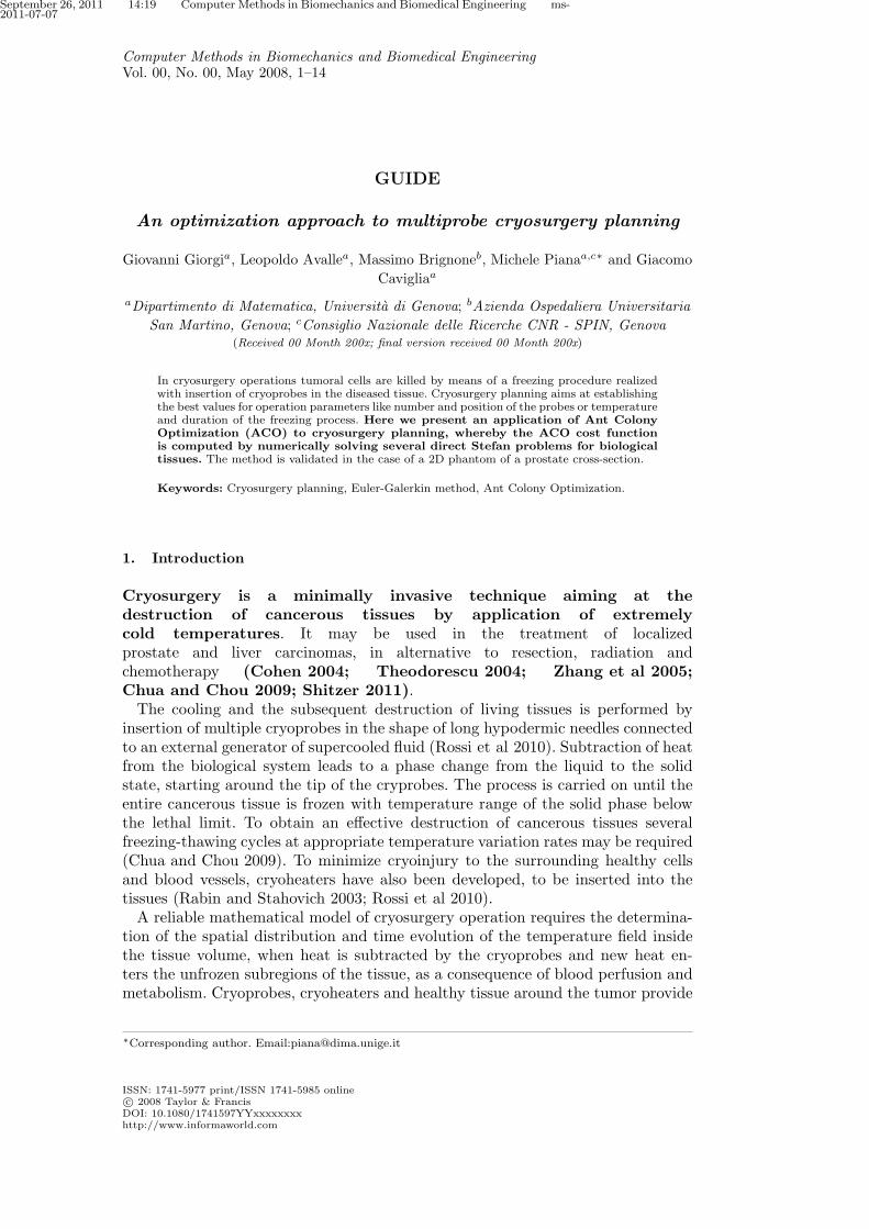
∂ E∂ C∂ H

V3

V1

V2

θ=θM

θ=θm

Figure 1. Scheme of a generic cryosurgery experiment: four cryoprobes (circles) and two cryoheaters(circles with crosses).

Therefore equations (1), (2) and (5) may be reformulated in the equivalent compactform

a(θ)∂θ

∂t= ∇ · (k(θ)∇θ) + b(θ) (9)

in the fixed open volume V = V1 ∪ V2 ∪ V3.Denote by ∂C, ∂H and ∂E the union of the boundaries of all cryoprobes, all

cryoheaters, and the external boundary between V and healthy tissues (see Figure1), respectively. Boundary and initial conditions of (9) are set as θ(x, t) = α(t) x ∈ ∂C, t > 0

θ(x, t) = 37oC x ∈ ∂H ∪ ∂E, t > 0θ(x, 0) = 37oC x ∈ V.

(10)

Here α is a given function of time expressing the decay law of the temperature of thecryoprobes: to simplify we have considered the same decay law for all cryoprobes,although the algorithm works as well if the decay law changes with the cryoprobe.

3. Numerical solution of the direct Stefan problem

The problem of finding the temperature distribution determined by a group of coldand hot cryoprobes of given positions and temperature laws is solved by an Euler-Galerkin approach, i.e. a method combining a finite difference approximation ofthe time-derivative and a finite element approach solving the space dependent partof the differential problem (9)-(10).The approximation scheme is iterative in time. If TM is the duration of the

cryosurgery experiment and ∆t = TM/n is the time step, at each iteration τ =0, 1, ... we set

∂

∂tθτ+1 ≈

1

∆t(θτ+1 − θτ ). (11)



The functions a, k, and b are defined at every step of the iterative process interms of the value of the temperature distribution at the previous step. Furthercomparison with (11), shows that equation (9) can be approximated by

a(θτ )

∆t(θτ+1 − θτ ) = ∇ · (k(θτ )∇(θτ+1)) + χ(θτ )b(θτ+1) (12)

where θτ is given and θτ+1 is the unknown. Integration of (12) against test functionsϕ ∈ H1

0 (V ) and use of the Green’s identity lead to the variational formulation∫Va(θτ )

θτ+1 − θτ∆t

ϕ dv =

=

∫V[−k(θτ )∇ϕ · ∇θτ+1 + b(θτ+1)ϕ] dv. (13)

The finite element approximation of (12) is based on (13), where boundary con-ditions (10) are imposed through penalization (Allaire 2007).

Given an operation time TM , the Euler-Galerkin approach provides an approxi-mation of the temperature distribution during the evolution from t = 0 to t = TM .The effectiveness of the cryosurgery simulation can be quantitatively assessed byintroducing a simple cost function that counts one all defective pixels andzero all correctly treated pixels (i.e. all pixels in the tumoral regionwhose temperature is higher than a reference temperature and all thepixels in the healthy tissue whose temperature is smaller than this ref-erence temperature). More formally, a specific configuration of the cryosurgerydesign is represented by a state variable U, which is a list set? of N operatingparameters (e.g. number and position of cryoprobes, temperature variation, etc.)whose admissible values are contained in S ⊂ IRN . The cost function is the defectweight function F : S → IN such that

F(θU) =

∫Vµ(θU(x))dx (14)

where θU is the temperature distribution associated to U and

µ(θ(x)) :=

0 if θ(x) < θ and x is diseased1 if θ(x) < θ and x is healthy1 if θ(x) ≥ θ and x is diseased0 if θ(x) ≥ θ and x is healthy.

(15)

The most appropriate choice of the constant reference temperature θis discussed in (Lung et al 2004), where the defect weight function wasfirst introduced. In our applications we have used θ = −22oC as suggestedin that paper. The cost function (14) plays a central role in the optimizationprocedure for the cryosurgery planning.

4. ACO optimization procedure

Ant Colony Optimization (ACO) is a statistical based optimization method de-veloped in the nineties with the aim of providing, in a limited amount of time,



a reliable although not optimal solution to some NP-hard combinatorial opti-mization problems. More recently, ACO has been generalized to continuous do-mains (Socha and Dorigo 2003). In view of its generality and wide range of ap-plicability, ACO has been successfully applied to a wide range of problems (e.g.(Brignone et al 2008), (Dorigo and Gambardella 1997)).ACO takes inspiration from the way in which ants find and carry food to their

nest. While an ant is going back to the nest after having taken some food, itreleases a pheromone trace: this trace serves as a trail for next ants, which are ableto reach food detecting pheromone. Since the pheromone decays in time, its densityis higher if the path to food is shorter and more crowded; on the other hand, morepheromone attracts more ants, making longer paths to be forgotten until, at theend, all ants follow the same trail.Ants’ behavior is paraphrased in ACO identifying the cost function F with the

length of the path to food, and the pheromone traces with a probability densitywhich is updated at each iteration depending on the value of the cost function fora set of states. In practice, at each iteration, the cost function is evaluated on a setof P admissible states, and the states are ordered according to increasing values ofthe cost function. Then ACO defines a probability distribution which is more densein correspondence of the cheaper states (i.e. the states with smallest values for F)and, on its basis, Q new states are extracted; a comparison procedure identifies thenew best P states which form the next set of states.In more details, the starting point of the algorithm is a set of P states,

B := {Uk = (u1,k, ..., uN,k), such that

Uk ∈ S ⊂ IRN , k = 1, . . . , P} (16)

that are ordered in terms of growing cost, namely, F(θU1) ≤ · · · ≤ F(θUP

).Next, for any j = 1, . . . , N e i = 1, . . . , P , one computes the parameters

mi,j = uj,i, si,j =ξ

P − 1

P∑p=1

|uj,p − uj,i|

and defines the Probability Density Function (PDF)

Gj(t) =P∑i=1

wiN[mi,j ,si,j ](t)

where N[µ,σ](t) is a Gaussian function with mean value µ and standard deviationσ and

wi = N[1,qP ](i) (17)

with i = 1, . . . , P and ξ, q real positive parameters to be fixed.It follows that Gj is a superposition of normal PDFs, each one of mean uj,i

and of variance si,j proportional to the average distance between uj,i and thecorresponding degrees of freedom of the other P configurations.By sampling S with Gj Q times, the procedure generates Q new states

UP+1, ...,UP+Q enlarging the set B to the set of states B := {U1, ...,UP+Q}.



If Uk1, ...,UkQ

are the Q states of B of greatest cost, the updated B is defined as

B = B \ {Uk1, ...,UkQ

}.

This procedure converges to an optimal solution of the problem by exploitingthe fact that the presence of weights wi in the definition of Gj gives emphasis tosolutions of lower costs since w1 > · · · > wP . This fact, associated to the influencethat a proper choice of parameters ξ and q has on the shape of the Gaussianfunctions, determines the way in which the method tunes the impact of the worseand best solutions.The algorithm ends when the difference between any two states of B is less

than a predefined quantity or when the maximum allowable number of iterations isreached. The initial set B of trial states is chosen by sampling a uniform probabilitydistribution.

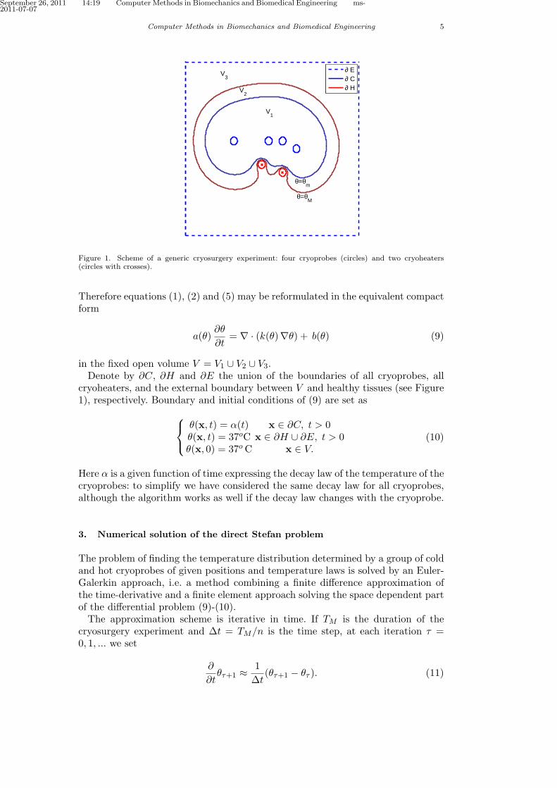
5. Numerical Examples

In this Section the optimization method is tested against the same 2D prostatephantom used in (Lung et al 2004) (see Figure 2).

−0.03 −0.02 −0.01 0 0.01 0.02 0.03−0.03

−0.02

−0.01

0

0.01

0.02

0.03

m

m

Figure 2. Prostate phantom used for numerical tests. Dashed lines delimit the area under investigation;the smallest circle inside the biggest one identify the urethra contour. The same phantom has beenused in (Lung et al 2004).

The optimization process is performed minimizing (14) on a square contain-ing the phantom and discretized by a grid of 1 mm x 1 mm pixels. Given aconfiguration of cryoprobes, the distribution of temperature is computed throughthe open source software FreeFem++ (Pironneau et al). The initial temperatureis set to 37 oC everywhere and cryoprobes are supposed to reach −145 oC in30 seconds; the temperature at the boundary of the urethra is set at 37 oC(see (Rabin and Stahovich 2003)) and external Dirichlet conditions are given ona square of side 0.1 m embedding the investigation domain. Phase change regionV2 is identified as the set of pixels of temperature between θm = −6 oC and θM = 0oC while the threshold value θ is −22 oC (see (Lung et al 2004)); cryoprobes aswell as cryoheaters have a circular cross-section with diameter of 1 mm. The othervalues are chosen according to Table 1.



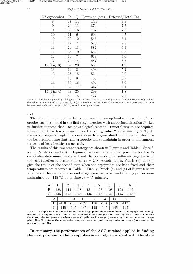
In the first numerical example we look for both the optimal position of a setof cryoprobes and the optimal duration of the cryosurgery experiment, (i.e. nocryoheaters are considered). Results are shown in Figures 3 - 4 and in Table 2where the behavior of the method is tested for different numbers of cryoprobes andfor different values of ACO’s parameters P and Q (P is chosen as multiple of thenumber of probes +1 whereas Q = [P2 ]+1 where [·] denotes the floor function). Thevalue of F(Uopt), with Uopt optimal configurations, generally decreases as P andQ increase, although some exception to this trend can occur due to the completerandomness of the initialization of the method.It is interesting to note that the level curve distribution in Figure 3

(c) implies a gradient of temperature from −45oC to +37oC (on the ure-thra boundary) over a very small distance (around 2 mm). This abruptbehavior is difficult to realize in a real experiment. However, this draw-back is not due to the optimization method but to the simplistic modeladopted, particularly in the definition of the boundary conditions. Theaim of our paper is to assess the reliability of a novel computational ap-proach in the case of a model widely adopted in the scientific literature.We also point out that one of the strengths of this approach is that thegeneralization to more realistic models is straightforward.

Parameters Units of measurements Valuesk1 W/(oC ·m) 1.76k3 W/(oC ·m) 0.50ρ1c1 MJ/(oC ·m3) 1.67ρ3c3 MJ/(oC ·m3) 3.35ρbwbcb kW/(oC ·m3) 40qm kW/m3 33.8θb

oC 37L MJ/m3 300

Table 1. Model parameters used in the numerical procedure.

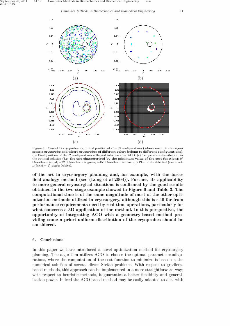
In the second experiment we consider the presence of cryoheaters as well ascryoprobes. Figure 5 shows the optimal solution of an experiment in which 14cryoprobes and 3 cryoheaters have to be placed and an optimal duration has tobe set: cryoprobes are constrained to fall inside the prostate, while cryoheaters areplaced outside the prostate, at the same side of the urethra. Again, ACO convergesto a configuration which guaranties the death of most the tumoral tissue, keepinghealthy tissues over temperature θ (the ratio between defected and total pixels isequal to 3.2% and the duration of the experiment is set by ACO to 571 seconds).A last example shows the efficacy of our optimization method when it is applied

to a more complex operation planning characterized by two distinct stages. In thefirst one, we want to setup the probes position; in the second one, we want tocontrol the temperature of each cryoprobe in order that the cold front keeps onfreezing the tumoral cells without invading the healthy tissue. The introductionof such a second stage is motivated by the fact that, in order to kill a tumoralcell, one has to keep its temperature low enough for an appropriate amount oftime. Moreover, recent studies claimed that the killing power of cold is increasedwhen cells are subjected to several cycles of thaw and freeze (Gage and Baust 1998)and the duration of these cycles is generally decided by medical doctors based onphysiological considerations. These facts can consistently increase the duration ofthe operation beyond the time established by the first stage and hence a manner tocontrol the ice propagation during the extended time becomes an essential planning



No cryoprobes P Q Duration (sec) Defected/Total (%)8 27 14 1289 8.99 20 11 874 7.79 30 16 737 7.310 11 6 609 9.710 22 12 546 6.111 12 7 573 9.811 24 13 587 5.511 36 19 552 3.512 13 7 618 4.012 26 14 587 3.7

12 (Fig. 3) 39 20 586 1.913 14 8 493 5.213 28 15 524 2.914 15 8 456 5.714 30 16 494 3.015 32 17 347 2.1

15 (Fig. 4) 48 25 298 1.816 34 18 427 2.5

Table 2. Results for geometry of Figure 2 in the case of q = 0.05 and ξ = 0.5. Columns respectively collect

the values of: number of cryoprobes, P , Q (parameters of ACO), optimal duration for the experiment and ratio

between still defected area (i.e. F(Uopt)) and investigated area.

tool.Therefore, in more details, let us suppose that an optimal configuration of cry-

oprobes has been fixed in the first stage together with an optimal duration T1. Letus further suppose that - for physiological reasons - tumoral tissues are requiredto maintain their temperature under the killing value θ for a time T2 > T1. Inthe second stage our optimization approach is generalized to optimally determinethe best temperature that each cryoprobe has to maintain in order to kill tumoraltissues and keep healthy tissues safe.The results of this two-stage strategy are shown in Figure 6 and Table 3. Specif-

ically, Panels (a) and (b) in Figure 6 represent the optimal positions for the 15cryoprobes determined in stage 1 and the corresponding isotherms together withthe cost function representation at T1 = 298 seconds. Then, Panels (c) and (d)give the result of the second step when the cryoprobes are kept fixed and theirtemperatures are reported in Table 3. Finally, Panels (e) and (f) of Figure 6 showwhat would happen if the second stage were neglected and the cryoprobes weremaintained at −145 oC up to time T2 = 15 minutes.

A 1 2 3 4 5 6 7 8B -128 -114 -118 -134 -123 -128 -122 -112C -145 -145 -145 -145 -145 -145 -145 -145

A 9 10 11 12 13 14 15B -110 -138 -122 -128 -137 -113 -117C -145 -145 -145 -145 -145 -145 -145

Table 3. Temperature optimization in a two-stage planning (second stage): the cryoprobes’ config-

uration is in Figure 6 (c). Line A indicates the cryoprobe position (see Figure 6); line B contains

the cryoprobe temperature when a second optimization stage (concerning the temperature) is ap-

plied; line C contains the cryoprobe temperature when just one optimization stage (concerning the

position) is applied.

In summary, the performances of the ACO method applied in findingthe best position of the cryoprobes are nicely consistent with the state



(a) (b)

(c) (d)

Figure 3. Case of 12 cryoprobes. (a) Initial position of P = 39 configurations (where each circle repre-sents a cryoprobe and where cryoprobes of different colors belong to different configurations).(b) Final position of the P configurations collapsed into one after ACO. (c) Temperature distribution forthe optimal solution (i.e. the one characterized by the minimum value of the cost function): 0o

C-isotherm is red, −22o C-isotherm is green, −45o C-isotherm is blue. (d) Plot of the defected (i.e. x s.t.µ(θ(x)) = 1) pixels (white).

of the art in cryosurgery planning and, for example, with the force-field analogy method (see (Lung et al 2004)). Further, its applicabilityto more general cryosurgical situations is confirmed by the good resultsobtained in the two-stage example showed in Figure 6 and Table 3. Thecomputational time is of the same magnitude of most of the other opti-mization methods utilized in cryosurgery, although this is still far fromperformance requirements need by real-time operations, particularly forwhat concerns a 3D application of the method. In this perspective, theopportunity of integrating ACO with a geometry-based method pro-viding some a priori uniform distribution of the cryoprobes should beconsidered.

6. Conclusions

In this paper we have introduced a novel optimization method for cryosurgeryplanning. The algorithm utilizes ACO to choose the optimal parameter configu-rations, where the computation of the cost function to minimize is based on thenumerical solution of several direct Stefan problems. With respect to gradient-based methods, this approach can be implemented in a more straightforward way;with respect to heuristic methods, it guaranties a better flexibility and general-ization power. Indeed the ACO-based method may be easily adapted to deal with


12 REFERENCES

(a) (b)

(c) (d)

Figure 4. Case of 15 cryoprobes. (a) Initial position of P = 48 configurations (where each circle repre-sents a cryoprobe and where cryoprobes of different colors belong to different configurations).(b) Final position of the P configurations after ACO. (c) Temperature distribution for the optimal solution(i.e. the one characterized by the minimum value of the cost function): 0o C-isotherm is red,−22o C-isotherm is green, −45o C-isotherm is blue. (d) Plot of the defected (i.e. x s.t. µ(θ(x)) = 1) pixels(white).

a variety of parameters entering the numerical simulation of a cryosurgery exper-iment. Also, the parameters to be optimized may be divided into families to beprocessed in subsequent steps. Finally, if continuous functions are involved in thedescription of a state, they may be replaced by piecewise constant functions thusreducing the optimization problem to a finite number of degrees of freedom.There are no a priori restrictions on the choice of the independent initial states,

although common practice can suggest choices that may reduce the number ofiterations. Every iteration requires the solution of several direct independent Stefanproblems, but a notable saving of time may be achieved by parallelized computationthat can be very naturally realized.To simplify computations, in this paper we have been concerned with a 2D

domain, but the approach in terms of ACO can be straightforwardly generalized toa 3-dimensional framework. Similarly, more realistic models for the direct Stefanproblems can be considered where, e.g., the thermal conductivity of the solid phasedepends on the temperature. Freeze-thaw processes of different cooling rates canalso be considered for optimization. Also the definition of the cost function can bemodified to obtain a more accurate description of defective pixels.

References

[Allaire 2007] G. Allaire, ”Numerical Analysis and Optimization”, Oxford University Press, 2007.


REFERENCES 13

(a) (b)

(c) (d)

Figure 5. Case of 14 cryoprobes and 3 cryoheaters (where each circle represents a cryoprobe andwhere cryoprobes of different colors belong to different configurations); q = 0.015, ξ = 0.4,P = 36, Q = 19. (a) Initial position of the P configurations. (b) Final position of the P configurationsafter ACO. (c) Temperature distribution for the optimal solution (i.e. the one characterized by theminimum value of the cost function): 0o C-isotherm is red, −22o C-isotherm is green, −45o C-isothermis blue. (d) Plot of the defected (i.e. x s.t. µ(θ(x)) = 1) pixels (white).

[Bonacina et al 1973] C. Bonacina, G. Comini, A. Fasano, M. Primicerio, ”Numerical solution of phasechange problems”, Int. J. Heat Mass Transer 16, pp. 1825-1832, 1973.

[Brignone et al 2008] M. Brignone, G. Bozza, A. Randazzo, M. Piana, M. Pastorino, ”A Hybrid Apprachto 3D Microwave Imaging by Using Linear Sampling Method and Ant Colony Optimization”, Ieee.Trans. Ant. Prop. 56, pp. 3224-3232, 2008.

[Baissalov et al 2000] R. Baissalov, G. A. Sandison, B. J. Donnelly, J. C. Saliken, J. G. McKinnon, K. Mul-drew, J. C. Rewcastle, ”A semi-empirical treatment planning model for optimization of multiprobecryosurgery”, Phys. Med. Biol. 45, pp. 1085-1098, 2000.

[Baissalov et al 2001] R. Baissalov, G. A. Sandison, D. Reynolds, K. Muldrew, ”Simultaneous optimizationof cryoprobe placement and thermal protocol for cryosurgery”, J. Water Health 46, pp. 1799-1814, 2001.

[Cohen 2004] J. K. Cohen, ”Cryosurgery of the prostate: techniques and indications”, Rev. Urol. 6, pp.S20-S26, 2004.

[Chua and Chou 2009] K. J. Chua, S. K. Chou, ”On the study of the freeze-thaw thermal process of abiological system”, Appl. Thermal Engin. 29, pp. 3696-3709, 2009.

[Dorigo and Gambardella 1997] M. Dorigo, L. M. Gambardella, ”Ant Colony System: A CooperativeLearning Approach to the Traveling Salesman Problem”, Ieee. Trans. Evol. Comp. 1, pp. 53-66, 1997.

[Gage and Baust 1998] A. A. Gage, J. Baust, ”Mechanisms of tissue injury in cryosurgery”, Cryobiology37, pp. 171-186, 1998.

[Keanini and Rubinsky 1992] R. G. Keanini, B. Rubinsky, ”Optimization of Multiprobe Cryosurgery”,ASME J. Heat Transfer 114, pp. 796-802, 1992.

[Lung et al 2004] D. C. Lung, T. F. Stahovic, Y. Rabin, ”Computerized Planning for MultiprobeCryosurgery using a Force-field Analogy”, Comp. Meth. in Biomech. and Biomed. Eng. 7, pp. 101-110,2004.

[Pennes 1948] H. H. Pennes, ”Analysis of tissue and arterial blood temperature in the resting humanfoream”, J. Appl. Phys. 1, pp. 93-122, 1948.

[Pironneau et al] O. Pironneau, F. Hecht, A. Le Hyaric, J. Morice, ”www.freefem.org/ff++/index.htm”.[Rabin et al 2004] J. Rabin, D. C. Lung, T. F. Stahovich, ”Computerized planning of cryosurgery using

cryoprobes and cryoheaters”, Technology and Cancer Research & Treatment 3, pp. 229-243, 2004.[Rabin and Shitzer 1998] Y. Rabin, A. Shitzer, ”Numerical solution of the multidimensional freezing prob-

lem during cryosurgery”, Trans. ASME 120, pp. 32-37, 1998.[Rabin and Stahovich 2003] Y. Rabin, T. F. Stahovich, ”Cryoheater as a means of cryosurgery control”,


14 REFERENCES

(a) (b)

(c) (d)

(e) (f)

Figure 6. Two stage planning: case of 15 cryoprobes, P = 48, Q = 25, q = 0.015, ξ = 0.5. (a) and (b)contain the first stage results (see Figure 4). (c) Temperature distribution after 15 minutes with cryoprobes’temperature optimization: 0o C-isotherm is red, −22o C-isotherm is green, −45o C-isotherm is blue. (d)Plot of the defected (i.e. x s.t. µ(θ(x)) = 1) pixels (white) with cryoprobes’ temperature optimization. (e)Temperature distribution after 15 minutes without cryoprobes’ temperature optimization: 0o C-isothermis red, −22o C-isotherm is green, −45o C-isotherm is blue. (f) Plot of the defected pixels (white) withoutcryoprobes’ temperature optimization.

Phys. Med. Biol. 48, pp. 619-632, 2003.[Rossi et al 2010] M. R. Rossi, D. Tanaka, K. Shimada, Y. Rabin, ”Computerized planning of prostate

cryosurgery using variable cryprobe insertion depth”, Cryobiology 60, pp. 71-79, 2010.[Rossi et al 2007] M. R. Rossi, D. Tanaka, K. Shimada, Y. Rabin, ”An efficient numerical technique for

bioheat simulations and its application to computerized cryosurgery planning”, Comp. Meth. Progr.Biomed. 85, pp. 41-50, 2007.

[Rossi et al 2008] M. R. Rossi, D. Tanaka, K. Shimada, Y. Rabin, ”Computerized planning of cryosurgeryusing bubble packing: an experimenthal validation on a phantom material”, Int. J. Heat Mass Tran.51, pp. 5671-5678, 2008.

[Shitzer 2011] A. Shitzer, ”Cryosurgery Analysis and Experimentation of Cryoprobes in Phase ChangingMedia”, J. Heat Transf. 133, pp. 011005-011017, 2011.

[Socha and Dorigo 2003] K. Socha, M. Dorigo, ”Ant colony optimization for continuous domains”, Eur.


REFERENCES 15

J. Oper. Res. 50, pp. 1180 - 1189, 2003.[Tanaka et al 2006] D. Tanaka, K. Shimada, Y. Rabin, ”Two-Phase Computerized Planning of

Cryosurgery Using Bubble-Packing and Force-Field Analogy”, J. Biomech. Engng. 128, pp. 49-58,2006.

[Theodorescu 2004] D. Theodorescu, ”Cancer cryotherapy: evolution and biology”, Rev. Urol. 6, pp. S9-S19, 2004.

[Zhang et al 2005] J. Zhang, G. A. Sandison, J. Y. Murthy, L. X. Xu, ”Numerical simulation for heattransfer in prostate cancer cryosurgery”, J. Biomech. Engin. 127, pp. 279-294, 2005.

[Zhao et al 2007] G. Zhao, H. Zhang, X. Guo, D. Luo, D. Gao, ”Effect of blood flow and metabolism onmultidimensional heat transfer during cryosurgery”, Med. Engng. and Phys. 29, pp. 205-215, 2007.

Documents

GUIDE An optimization approach to multiprobe cryosurgery ...mida.dima.unige.it/files/cryo.pdf · September 26, 2011 14:19 Computer Methods in Biomechanics and Biomedical Engineering