Embed Size (px)
Citation preview
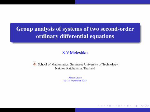
Group analysis of systems of two second-orderordinary differential equations
S.V.Meleshko
School of Mathematics, Suranaree University of Technology,Nakhon Ratchasima, Thailand
Abrao-Durso16–21 September 2013

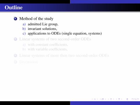
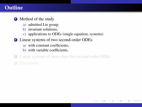
Outline
1 Method of the studya) admitted Lie group,b) invariant solutions,c) applications to ODEs (single equation, systems)
2 Linear systems of two second-order ODEsa) with constant coefficients,b) with variable coefficients,
3 Linear systems of more then two second-order ODEs4 Discussion
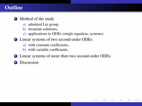
Outline
1 Method of the studya) admitted Lie group,b) invariant solutions,c) applications to ODEs (single equation, systems)
2 Linear systems of two second-order ODEsa) with constant coefficients,b) with variable coefficients,
3 Linear systems of more then two second-order ODEs4 Discussion
Outline
1 Method of the studya) admitted Lie group,b) invariant solutions,c) applications to ODEs (single equation, systems)
2 Linear systems of two second-order ODEsa) with constant coefficients,b) with variable coefficients,
3 Linear systems of more then two second-order ODEs4 Discussion

Outline
1 Method of the studya) admitted Lie group,b) invariant solutions,c) applications to ODEs (single equation, systems)
2 Linear systems of two second-order ODEsa) with constant coefficients,b) with variable coefficients,
3 Linear systems of more then two second-order ODEs4 Discussion
Outline
1 Method of the studya) admitted Lie group,b) invariant solutions,c) applications to ODEs (single equation, systems)
2 Linear systems of two second-order ODEsa) with constant coefficients,b) with variable coefficients,
3 Linear systems of more then two second-order ODEs4 Discussion

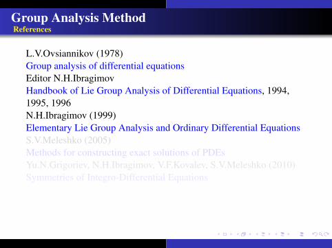
Group Analysis MethodReferences
L.V.Ovsiannikov (1978)Group analysis of differential equationsEditor N.H.IbragimovHandbook of Lie Group Analysis of Differential Equations, 1994,1995, 1996N.H.Ibragimov (1999)Elementary Lie Group Analysis and Ordinary Differential EquationsS.V.Meleshko (2005)Methods for constructing exact solutions of PDEsYu.N.Grigoriev, N.H.Ibragimov, V.F.Kovalev, S.V.Meleshko (2010)Symmetries of Integro-Differential Equations
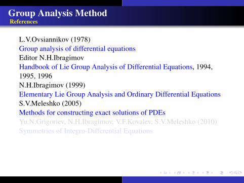

Group ClassificationLie Group of Transformations

Group ClassificationLie Group of Transformations

Group ClassificationInfinitesimal Generators

Group ClassificationInfinitesimal Generators

Group ClassificationGeneral Scheme for Finding Invariant Solutions
S(x, u, p) = 0
1. Find admitted Lie algebra.
2. Choose a subalgebra.
3. Find invariants of the subalgebra.
4. Construct a representation of an invariant or partially invariantsolution.
5. Substitute a representation of the solution into the original systemof differential equations.
6. Make a compatibility analysis of the reduced system

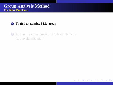
Group Analysis MethodThe Main Problems
1 To find an admitted Lie group
2 To classify equations with arbitrary elements(group classification)
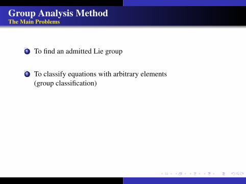
Group Analysis MethodThe Main Problems
1 To find an admitted Lie group
2 To classify equations with arbitrary elements(group classification)
Group Analysis MethodThe Main Problems
1 To find an admitted Lie group
2 To classify equations with arbitrary elements(group classification)

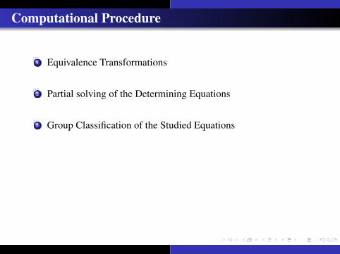
Computational Procedure
1 Equivalence Transformations
2 Partial solving of the Determining Equations
3 Group Classification of the Studied Equations

Computational Procedure
1 Equivalence Transformations
2 Partial solving of the Determining Equations
3 Group Classification of the Studied Equations
Computational Procedure
1 Equivalence Transformations
2 Partial solving of the Determining Equations
3 Group Classification of the Studied Equations

Computational Procedure
1 Equivalence Transformations
2 Partial solving of the Determining Equations
3 Group Classification of the Studied Equations
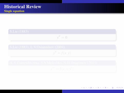
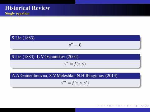
Historical ReviewSingle equation
S.Lie (1883)
y′′ = 0
S.Lie (1883), L.V.Osiannikov (2004)
y′′ = f (x, y)
A.A.Gainetdinovna, S.V.Meleshko, N.H.Ibragimov (2013)
y′′′ = f (x, y, y′)

Historical ReviewSingle equation
S.Lie (1883)
y′′ = 0
S.Lie (1883), L.V.Osiannikov (2004)
y′′ = f (x, y)
A.A.Gainetdinovna, S.V.Meleshko, N.H.Ibragimov (2013)
y′′′ = f (x, y, y′)

Historical ReviewSingle equation
S.Lie (1883)
y′′ = 0
S.Lie (1883), L.V.Osiannikov (2004)
y′′ = f (x, y)
A.A.Gainetdinovna, S.V.Meleshko, N.H.Ibragimov (2013)
y′′′ = f (x, y, y′)
Historical ReviewSingle equation
S.Lie (1883)
y′′ = 0
S.Lie (1883), L.V.Osiannikov (2004)
y′′ = f (x, y)
A.A.Gainetdinovna, S.V.Meleshko, N.H.Ibragimov (2013)
y′′′ = f (x, y, y′)

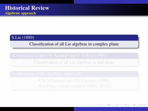
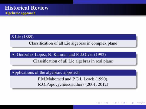
Historical ReviewAlgebraic approach
S.Lie (1889)Classification of all Lie algebras in complex plane
A. Gonzalez-Lopez, N. Kamran and P. J.Olver (1992)Classification of all Lie algebras in real plane
Applications of the algebraic approachF.M.Mahomed and P.G.L.Leach (1990),R.O.Popovych&coauthors (2001, 2012)

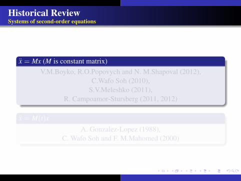
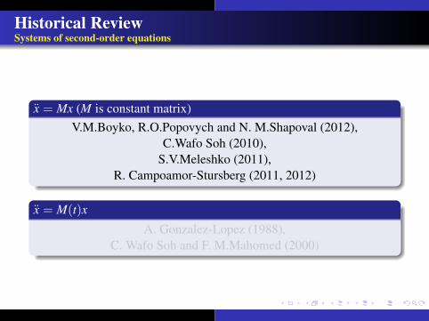
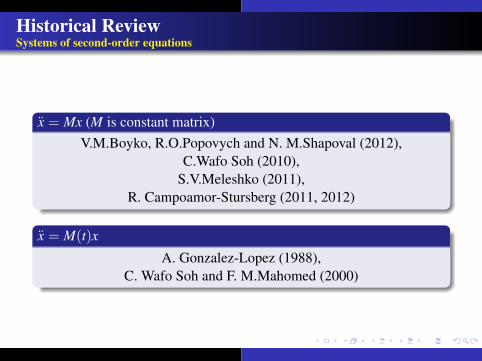
Historical ReviewSystems of second-order equations
x = Mx (M is constant matrix)V.M.Boyko, R.O.Popovych and N. M.Shapoval (2012),
C.Wafo Soh (2010),S.V.Meleshko (2011),
R. Campoamor-Stursberg (2011, 2012)
x = M(t)x
A. Gonzalez-Lopez (1988),C. Wafo Soh and F. M.Mahomed (2000)
Historical ReviewSystems of second-order equations
x = Mx (M is constant matrix)V.M.Boyko, R.O.Popovych and N. M.Shapoval (2012),
C.Wafo Soh (2010),S.V.Meleshko (2011),
R. Campoamor-Stursberg (2011, 2012)
x = M(t)x
A. Gonzalez-Lopez (1988),C. Wafo Soh and F. M.Mahomed (2000)

Historical ReviewSystems of second-order equations
x = Mx (M is constant matrix)V.M.Boyko, R.O.Popovych and N. M.Shapoval (2012),
C.Wafo Soh (2010),S.V.Meleshko (2011),
R. Campoamor-Stursberg (2011, 2012)
x = M(t)x
A. Gonzalez-Lopez (1988),C. Wafo Soh and F. M.Mahomed (2000)
Historical ReviewSystems of second-order equations
x = Mx (M is constant matrix)V.M.Boyko, R.O.Popovych and N. M.Shapoval (2012),
C.Wafo Soh (2010),S.V.Meleshko (2011),
R. Campoamor-Stursberg (2011, 2012)
x = M(t)x
A. Gonzalez-Lopez (1988),C. Wafo Soh and F. M.Mahomed (2000)
Historical ReviewSystems of second-order equations
x = Mx (M is constant matrix)V.M.Boyko, R.O.Popovych and N. M.Shapoval (2012),
C.Wafo Soh (2010),S.V.Meleshko (2011),
R. Campoamor-Stursberg (2011, 2012)
x = M(t)x
A. Gonzalez-Lopez (1988),C. Wafo Soh and F. M.Mahomed (2000)
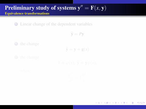
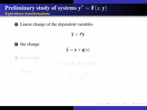
Preliminary study of systems y′′ = F(x, y)Equivalence transformations
1 Linear change of the dependent variables
y = Py
2 the changey = y + g(x)
3 the changex = ϕ(x), y = yψ(x),
whereϕ′′
ϕ′= 2
ψ′
ψ.

Preliminary study of systems y′′ = F(x, y)Equivalence transformations
1 Linear change of the dependent variables
y = Py
2 the changey = y + g(x)
3 the changex = ϕ(x), y = yψ(x),
whereϕ′′
ϕ′= 2
ψ′
ψ.
Preliminary study of systems y′′ = F(x, y)Equivalence transformations
1 Linear change of the dependent variables
y = Py
2 the changey = y + g(x)
3 the changex = ϕ(x), y = yψ(x),
whereϕ′′
ϕ′= 2
ψ′
ψ.

Preliminary study of systems y′′ = F(x, y)Equivalence transformations
1 Linear change of the dependent variables
y = Py
2 the changey = y + g(x)
3 the changex = ϕ(x), y = yψ(x),
whereϕ′′
ϕ′= 2
ψ′
ψ.

Preliminary study of systems y′′ = F(x, y)Equivalence transformations
1 Linear change of the dependent variables
y = Py
2 the changey = y + g(x)
3 the changex = ϕ(x), y = yψ(x),
whereϕ′′
ϕ′= 2
ψ′
ψ.

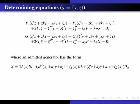
Determining equations (y = (y, z))
Fz(ξ′z + zk4 + yk3 + ζ2) + Fy(ξ
′y + zk2 + yk1 + ζ1)+2Fxξ − ξ′′′y + 3ξ′F − ζ ′′1 − k1F − k2G = 0,
Gz(ξ′z + zk4 + yk3 + ζ2) + Gy(ξ
′y + zk2 + yk1 + ζ1)+2Gxξ − ξ′′′z + 3ξ′G− ζ ′′2 − k3F − k4G = 0,
where an admitted generator has the form
X = 2ξ(x)∂x+(yξ′(x)+k1y+k2z+ζ1(x))∂y+(ξ′z+k3y+k4z+ζ2(x))∂z,
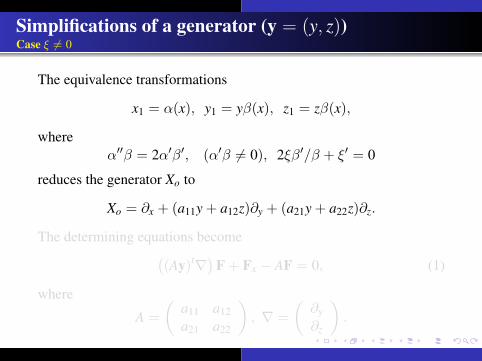
Simplifications of a generator (y = (y, z))Case ξ 6= 0
The equivalence transformations
x1 = α(x), y1 = yβ(x), z1 = zβ(x),
whereα′′β = 2α′β′, (α′β 6= 0), 2ξβ′/β + ξ′ = 0
reduces the generator Xo to
Xo = ∂x + (a11y + a12z)∂y + (a21y + a22z)∂z.
The determining equations become((Ay)t∇
)F + Fx − AF = 0, (1)
where
A =
(a11 a12a21 a22
), ∇ =
(∂y
∂z
).
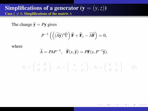
Simplifications of a generator (y = (y, z))Case ξ 6= 0. Simplifications of the matrix A
The change y = Py gives
P−1((
(Ay)t∇)
F + Fx − AF)
= 0,
whereA = PAP−1, F(x, y) = PF(x,P−1y).
J1 =
(a 00 b
), J2 =
(a c−c a
), J3 =
(a 10 a
), (2)

Simplifications of a generator (y = (y, z))Case ξ 6= 0. Simplifications of the matrix A
The change y = Py gives
P−1((
(Ay)t∇)
F + Fx − AF)
= 0,
whereA = PAP−1, F(x, y) = PF(x,P−1y).
J1 =
(a 00 b
), J2 =
(a c−c a
), J3 =
(a 10 a
), (2)

Simplifications of a generator (y = (y, z))Case ξ 6= 0 and A = J1
ayFy + bzFz + Fx = aF,ayGy + bzGz + Gx = bG.
The general solution of these equations is
F(x, u, v) = eaxf (u, v), G(x, u, v) = ebxg(u, v)
u = ye−ax, v = ze−bx.
Xo = ∂x + ay∂y + bz∂z.

Simplifications of a generator (y = (y, z))Case ξ 6= 0 and A = J2
F(x, u, v) = eax (cos(cx)f (u, v) + sin(cx)g(u, v)) ,G(x, y, z) = eax (− sin(cx)f (u, v) + cos(cx)g(u, v))
u = e−ax(y cos(cx)− z sin(cx)), v = e−ax(y sin(cx) + z cos(cx)),
Xo = ∂x + (ay + cz)∂y + (−cy + az)∂z.
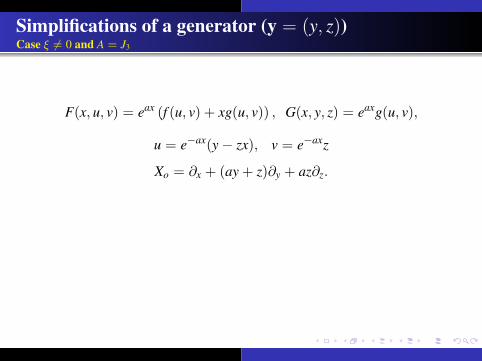
Simplifications of a generator (y = (y, z))Case ξ 6= 0 and A = J3
F(x, u, v) = eax (f (u, v) + xg(u, v)) , G(x, y, z) = eaxg(u, v),
u = e−ax(y− zx), v = e−axz
Xo = ∂x + (ay + z)∂y + az∂z.
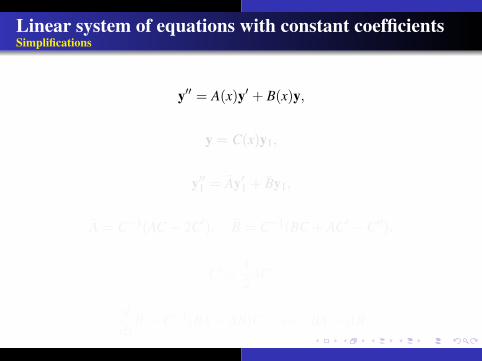
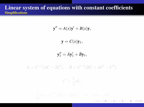
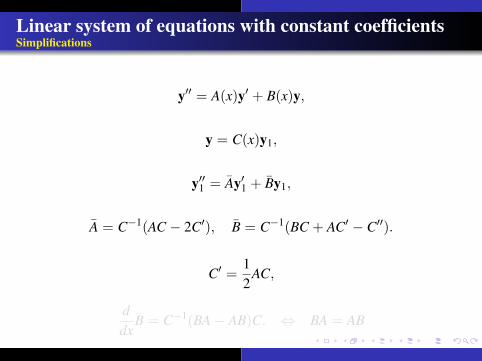
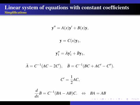
Linear system of equations with constant coefficientsSimplifications
y′′ = A(x)y′ + B(x)y,
y = C(x)y1,
y′′1 = Ay′1 + By1,
A = C−1(AC − 2C′), B = C−1(BC + AC′ − C′′).
C′ =12
AC,
ddx
B = C−1(BA− AB)C. ⇔ BA = AB

Linear system of equations with constant coefficientsSimplifications
y′′ = A(x)y′ + B(x)y,
y = C(x)y1,
y′′1 = Ay′1 + By1,
A = C−1(AC − 2C′), B = C−1(BC + AC′ − C′′).
C′ =12
AC,
ddx
B = C−1(BA− AB)C. ⇔ BA = AB
Linear system of equations with constant coefficientsSimplifications
y′′ = A(x)y′ + B(x)y,
y = C(x)y1,
y′′1 = Ay′1 + By1,
A = C−1(AC − 2C′), B = C−1(BC + AC′ − C′′).
C′ =12
AC,
ddx
B = C−1(BA− AB)C. ⇔ BA = AB

Linear system of equations with constant coefficientsSimplifications
y′′ = A(x)y′ + B(x)y,
y = C(x)y1,
y′′1 = Ay′1 + By1,
A = C−1(AC − 2C′), B = C−1(BC + AC′ − C′′).
C′ =12
AC,
ddx
B = C−1(BA− AB)C. ⇔ BA = AB
Linear system of equations with constant coefficientsSimplifications
y′′ = A(x)y′ + B(x)y,
y = C(x)y1,
y′′1 = Ay′1 + By1,
A = C−1(AC − 2C′), B = C−1(BC + AC′ − C′′).
C′ =12
AC,
ddx
B = C−1(BA− AB)C. ⇔ BA = AB
Linear system of equations with constant coefficientsSimplifications
y′′ = A(x)y′ + B(x)y,
y = C(x)y1,
y′′1 = Ay′1 + By1,
A = C−1(AC − 2C′), B = C−1(BC + AC′ − C′′).
C′ =12
AC,
ddx
B = C−1(BA− AB)C. ⇔ BA = AB

Linear system of equations with constant coefficientsNoncommutative matrices
Theorem. A linear system with non-commuting constant matrices Aand B admits a nontrivial symmetry if this system is equivalent to alinear system with the matrices A and B of the form
A =
(0 00 4
), B =
(b22 + 4 b12
0 b22
), (b12 6= 0). (3)
The admitting symmetries (except generic) of the system withmatrices (3) are
if b22 6= −15/4 : X1 = e−2xz∂y;
if b22 = −15/4 : X1 = e−2xz∂y,X2 = e−x (2∂x − y∂y + 3z∂z) .

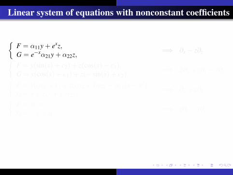
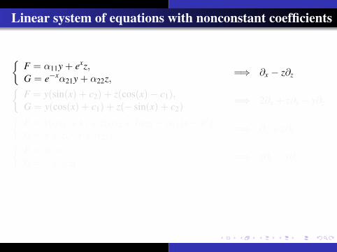
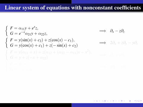
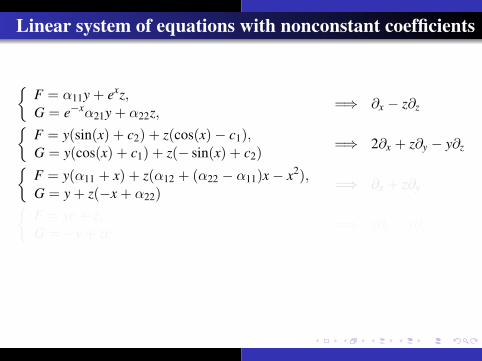
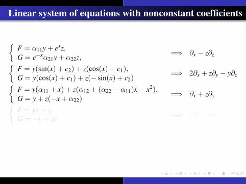
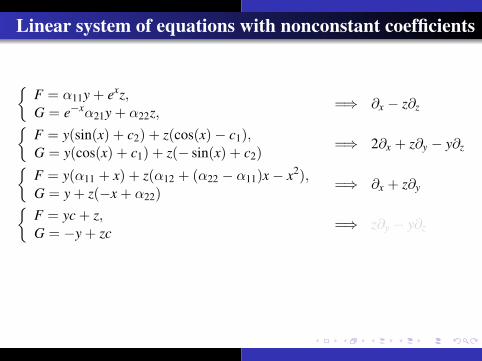
Linear system of equations with nonconstant coefficients
{F = α11y + exz,G = e−xα21y + α22z,
=⇒ ∂x − z∂z{F = y(sin(x) + c2) + z(cos(x)− c1),G = y(cos(x) + c1) + z(− sin(x) + c2)
=⇒ 2∂x + z∂y − y∂z{F = y(α11 + x) + z(α12 + (α22 − α11)x− x2),G = y + z(−x + α22)
=⇒ ∂x + z∂y{F = yc + z,G = −y + zc
=⇒ z∂y − y∂z

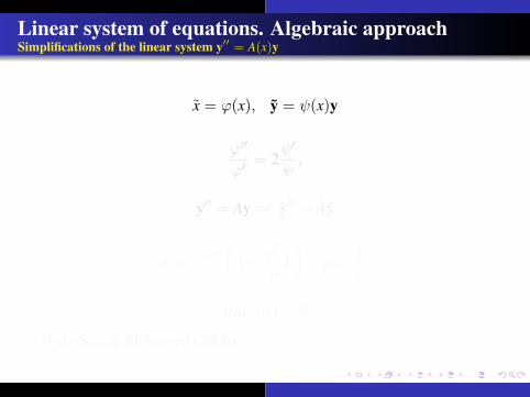
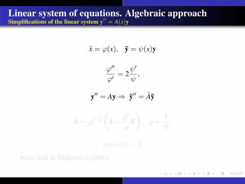
Linear system of equations. Algebraic approachSimplifications of the linear system y′′ = A(x)y
x = ϕ(x), y = ψ(x)y
ϕ′′
ϕ′= 2
ψ′
ψ,
y′′ = Ay⇒ y′′ = Ay
A = ϕ′−2(
A− ρ′′
ρE), ρ =
1ψ.
trace(A) = 0
Wafo Soh & Mahomed (2000)
Linear system of equations. Algebraic approachSimplifications of the linear system y′′ = A(x)y
x = ϕ(x), y = ψ(x)y
ϕ′′
ϕ′= 2
ψ′
ψ,
y′′ = Ay⇒ y′′ = Ay
A = ϕ′−2(
A− ρ′′
ρE), ρ =
1ψ.
trace(A) = 0
Wafo Soh & Mahomed (2000)

Linear system of equations. Algebraic approachSimplifications of the linear system y′′ = A(x)y
x = ϕ(x), y = ψ(x)y
ϕ′′
ϕ′= 2
ψ′
ψ,
y′′ = Ay⇒ y′′ = Ay
A = ϕ′−2(
A− ρ′′
ρE), ρ =
1ψ.
trace(A) = 0
Wafo Soh & Mahomed (2000)

Linear system of equations. Algebraic approachSimplifications of the linear system y′′ = A(x)y
x = ϕ(x), y = ψ(x)y
ϕ′′
ϕ′= 2
ψ′
ψ,
y′′ = Ay⇒ y′′ = Ay
A = ϕ′−2(
A− ρ′′
ρE), ρ =
1ψ.
trace(A) = 0
Wafo Soh & Mahomed (2000)
Linear system of equations. Algebraic approachSimplifications of the linear system y′′ = A(x)y
x = ϕ(x), y = ψ(x)y
ϕ′′
ϕ′= 2
ψ′
ψ,
y′′ = Ay⇒ y′′ = Ay
A = ϕ′−2(
A− ρ′′
ρE), ρ =
1ψ.
trace(A) = 0
Wafo Soh & Mahomed (2000)

Linear system of equations. Algebraic approachSimplifications of the linear system y′′ = A(x)y
x = ϕ(x), y = ψ(x)y
ϕ′′
ϕ′= 2
ψ′
ψ,
y′′ = Ay⇒ y′′ = Ay
A = ϕ′−2(
A− ρ′′
ρE), ρ =
1ψ.
trace(A) = 0
Wafo Soh & Mahomed (2000)

Linear system of equations. Algebraic approachSimplifications of the linear system y′′ = A(x)y
x = ϕ(x), y = ψ(x)y
ϕ′′
ϕ′= 2
ψ′
ψ,
y′′ = Ay⇒ y′′ = Ay
A = ϕ′−2(
A− ρ′′
ρE), ρ =
1ψ.
trace(A) = 0
Wafo Soh & Mahomed (2000)
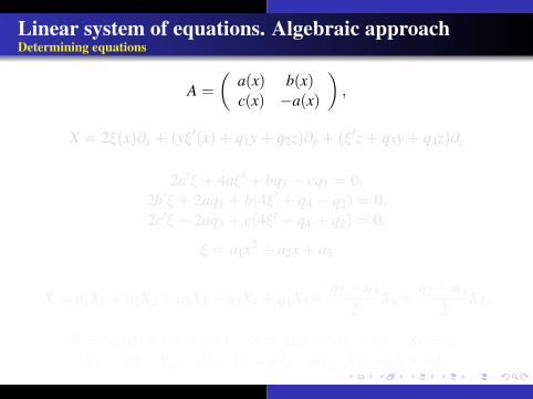
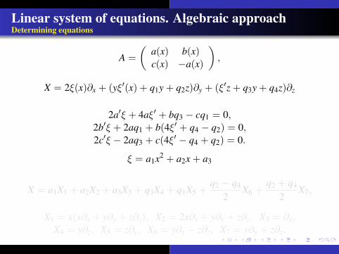
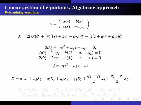
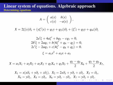
Linear system of equations. Algebraic approachDetermining equations
A =
(a(x) b(x)c(x) −a(x)
),
X = 2ξ(x)∂x + (yξ′(x) + q1y + q2z)∂y + (ξ′z + q3y + q4z)∂z
2a′ξ + 4aξ′ + bq3 − cq1 = 0,2b′ξ + 2aq1 + b(4ξ′ + q4 − q2) = 0,2c′ξ − 2aq3 + c(4ξ′ − q4 + q2) = 0.
ξ = a1x2 + a2x + a3
X = a1X1 + a2X2 + a3X3 + q3X4 + q1X5 +q2 − q4
2X6 +
q2 + q4
2X7,
X1 = x(x∂x + y∂y + z∂z), X2 = 2x∂x + y∂y + z∂z, X3 = ∂x,X4 = y∂z, X5 = z∂y, X6 = y∂y − z∂z, X7 = y∂y + z∂z.

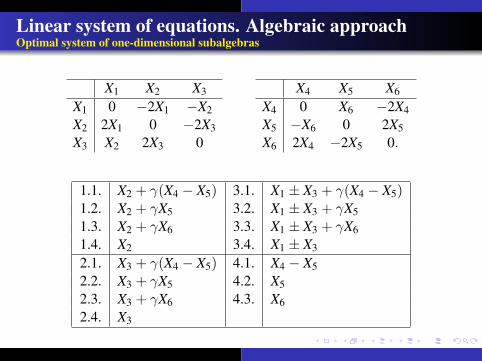
Linear system of equations. Algebraic approachOptimal system of one-dimensional subalgebras
X1 X2 X3
X1 0 −2X1 −X2X2 2X1 0 −2X3X3 X2 2X3 0
X4 X5 X6
X4 0 X6 −2X4X5 −X6 0 2X5X6 2X4 −2X5 0.
1.1. X2 + γ(X4 − X5) 3.1. X1 ± X3 + γ(X4 − X5)1.2. X2 + γX5 3.2. X1 ± X3 + γX51.3. X2 + γX6 3.3. X1 ± X3 + γX61.4. X2 3.4. X1 ± X3
2.1. X3 + γ(X4 − X5) 4.1. X4 − X52.2. X3 + γX5 4.2. X52.3. X3 + γX6 4.3. X62.4. X3
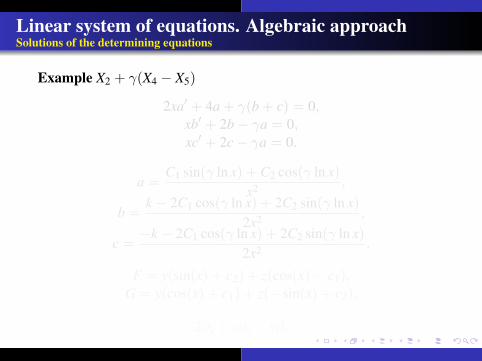
Linear system of equations. Algebraic approachSolutions of the determining equations
Example X2 + γ(X4 − X5)
2xa′ + 4a + γ(b + c) = 0,xb′ + 2b− γa = 0,xc′ + 2c− γa = 0.
a =C1 sin(γ ln x) + C2 cos(γ ln x)
x2 ,
b =k − 2C1 cos(γ ln x) + 2C2 sin(γ ln x)
2x2 ,
c =−k − 2C1 cos(γ ln x) + 2C2 sin(γ ln x)
2x2 .
F = y(sin(x) + c2) + z(cos(x)− c1),G = y(cos(x) + c1) + z(− sin(x) + c2),
2∂x + z∂y − y∂z
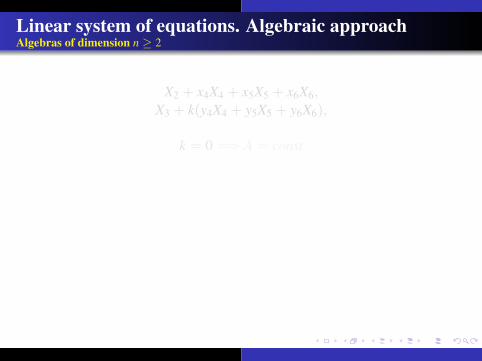
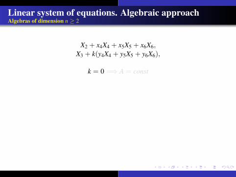
Linear system of equations. Algebraic approachAlgebras of dimension n ≥ 2
X2 + x4X4 + x5X5 + x6X6,X3 + k(y4X4 + y5X5 + y6X6),
k = 0 =⇒ A = const

Linear system of equations. Algebraic approachAlgebras of dimension n ≥ 2
X2 + x4X4 + x5X5 + x6X6,X3 + k(y4X4 + y5X5 + y6X6),
k = 0 =⇒ A = const
Linear system of equations. Algebraic approachAlgebras of dimension n ≥ 2
X2 + x4X4 + x5X5 + x6X6,X3 + k(y4X4 + y5X5 + y6X6),
k = 0 =⇒ A = const

Linear system of equations. Algebraic approachAlgebras of dimension n ≥ 2
X2 + x4X4 + x5X5 + x6X6,X3 + k(y4X4 + y5X5 + y6X6),
k = 0 =⇒ A = const

Linear system of three equations
y′′
z′′
u′′
=
a11(x) a12(x) a13(x)a21(x) a22(x) a23(x)a31(x) a32(x) a33(x)
yzu

References
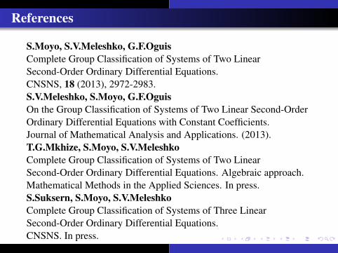
S.Moyo, S.V.Meleshko, G.F.OguisComplete Group Classification of Systems of Two LinearSecond-Order Ordinary Differential Equations.CNSNS, 18 (2013), 2972-2983.S.V.Meleshko, S.Moyo, G.F.OguisOn the Group Classification of Systems of Two Linear Second-OrderOrdinary Differential Equations with Constant Coefficients.Journal of Mathematical Analysis and Applications. (2013).T.G.Mkhize, S.Moyo, S.V.MeleshkoComplete Group Classification of Systems of Two LinearSecond-Order Ordinary Differential Equations. Algebraic approach.Mathematical Methods in the Applied Sciences. In press.S.Suksern, S.Moyo, S.V.MeleshkoComplete Group Classification of Systems of Three LinearSecond-Order Ordinary Differential Equations.CNSNS. In press.
References
S.Moyo, S.V.Meleshko, G.F.OguisComplete Group Classification of Systems of Two LinearSecond-Order Ordinary Differential Equations.CNSNS, 18 (2013), 2972-2983.S.V.Meleshko, S.Moyo, G.F.OguisOn the Group Classification of Systems of Two Linear Second-OrderOrdinary Differential Equations with Constant Coefficients.Journal of Mathematical Analysis and Applications. (2013).T.G.Mkhize, S.Moyo, S.V.MeleshkoComplete Group Classification of Systems of Two LinearSecond-Order Ordinary Differential Equations. Algebraic approach.Mathematical Methods in the Applied Sciences. In press.S.Suksern, S.Moyo, S.V.MeleshkoComplete Group Classification of Systems of Three LinearSecond-Order Ordinary Differential Equations.CNSNS. In press.


![Solution of Some Second Order Ordinary Differential ... · value problem of ordinary differential equations with a particular basis function was carried out by [1] which was improved](https://img.dokumen.tips/doc/110x75/5d5c255b88c993d2318b964a/solution-of-some-second-order-ordinary-differential-value-problem-of-ordinary.jpg)