Embed Size (px)
Citation preview
Grounded by Gravity:A Well-Behaved Trade Model with Industry-Level
Economies of Scale∗
Konstantin Kucheryavyy
U Tokyo
Gary Lyn
UMass Lowell
Andres Rodrıguez-Clare
UC Berkeley and NBER
September 19, 2016
Abstract
Although economists have long been interested in the implications of Marshal-lian externalities (i.e., industry-level external economies of scale) for trading econo-mies, the large number of equilibria that they typically imply has kept such exter-nalities out of the recent quantitative trade literature. This paper presents a multi-industry trade model with industry-level economies of scale that nests a Ricardianmodel with Marshallian externalities as well as multi-industry versions of Krugman(1980) and Melitz (2003). The behavior of the model depends on two industry-levelelasticities: the trade elasticity and the scale elasticity. We show that there is a uniqueequilibrium if the product of the trade and scale elasticities is weakly lower than onein all industries. The welfare analysis reveals that if this condition is satisfied thenall countries gain from trade, even when the scale elasticity varies across industries.The presence of scale economies tends to lower the gains from trade except if thecountry specializes in industries with relatively high scale elasticities. On the otherhand, scale economies amplify the gains from trade liberalization except if it leadsto reallocation towards industries with relatively low scale elasticities.
∗We thank James Anderson, Costas Arkolakis, Gaurab Aryal, Lorenzo Caliendo, Arnaud Costinot,Richard Cottle, Svetlana Demidova, Dave Donaldson, Jonathan Eaton, Gene Grossman, Nail Kashaev,Tim Kehoe, Hideo Konishi, Sam Kortum, Beresford Parlett, Donald Richards, Steve Redding, Michael Tsat-someros, Guang Yang, Xi Yang, and Stephen Yeaple for valuable discussions, and Kala Krishna for point-ing us back to perfect competition. We thank Mauricio Ulate and Piyush Panigrahi for valuable researchassistance. All errors are, of course, our own.
GROUNDED BY GRAVITY 1
1. Introduction
The field of international trade has made great strides in recent years by “mapping the-
ory to data” in the new quantitative trade models (or so-called “gravity models”). This
has led to important insights into the consequences of globalization. But a fundamen-
tal issue has been missing from these models: the role of localized and industry-specific
external economies of scale. These externalities played a large role in the world econ-
omy at the time of Marshall (1890, 1930), and recent anecdotal and empirical evidence
suggests that they play, if anything, an even larger role in the global economy today.1
There is good reason for this oversight. Early models yielded some discomforting re-
sults, including “a bewildering variety of [multiple] equilibria” (Krugman, 1995) so that
trade patterns need not conform to comparative advantage, along with the “paradoxi-
cal implication that trade motivated by the gains from concentrating production need
not benefit the participating countries” (Grossman and Rossi-Hansberg, 2010). At the
heart of these “pathologies” seemed to lay the compatibility assumption of increasing
returns and perfect competition (see Chipman, 1965), namely that firms take produc-
tivity as given even though productivity depends on total industry output. This leads to
a circularity whereby the scale of an industry affects its productivity, while an industry’s
productivity affects its scale through the impact on the pattern of comparative advan-
tage and specialization. In the standard analysis, this leads to multiple equilibria.2
Grossman and Rossi-Hansberg (2010, henceforth GRH) recently proposed a two-
country Ricardian model with national industry-level external economies of scale (or
Marshallian externalities), which attacks this compatibility assumption head-on. In-
stead of perfect competition, GRH assume Bertrand competition so that firms in each
industry understand the implications of their decisions on industry output and pro-
ductivity, ensuring that in equilibrium we have the “right” allocation of industries across
countries in a similar fashion to that of the constant returns to scale framework of Dorn-
busch, Fischer and Samuelson (1977). While the framework successfully eliminates the
“pathologies” in a world free of trade costs, Lyn and Rodrıguez-Clare (2013a,b) illus-
trate circumstances under which multiple equilibria arise in the presence of trade costs.
Coupled with the fact that the equilibrium has mixed strategies for some levels of trade
1See Krugman (2011) for a nice exposition of recent anecdotal evidence. For empirical evidence see,for instance, Caballero and Lyons (1989, 1990, 1992), Chan, Chen and Cheung (1995), Segoura (1998), andHenriksen, Steen and Ulltveit-Moe (2001).
2See early work exploring this by Graham (1923), Ohlin (1933), Matthews (1949), Kemp (1964), Melvin(1969), Markusen and Melvin (1981), and Ethier (1982a,b).

2 KUCHERYAVYY-LYN-RODRıGUEZ-CLARE
costs, the framework quickly becomes intractable, with little hope of extending it to a
multi-country setting with trade frictions.
In this paper we present a Ricardian model with Marshallian externalities that admits
a unique equilibrium under intuitive parameter restrictions. Unlike GRH, we leave the
compatibility assumption intact and approach the problem from a different angle by
relaxing the implicit assumption in the standard framework (and in GRH) that firms
within each industry are producing a homogeneous good. In particular, we allow for
intra-industry heterogeneity as in Eaton and Kortum (2002, henceforth EK) and find
that this adds some “curvature” that helps in establishing uniqueness of equilibrium as
long as the strength of Marshallian externalities is “not too high”. The framework yields
the standard gravity-type equation and so provides a platform to assess quantitatively
the importance of these externalities for the welfare effects of trade.3
The system of equations that characterizes the equilibrium of the Ricardian multi-
industry model with Marshallian externalities turns out to be isomorphic to the equi-
librium system of a more general version of the multi-industry Krugman (1980) model
of product differentiation with internal economies of scale.4 The existence and unique-
ness result that we prove for our Ricardian setting can then be seamlessly applied to the
multi-industry Krugman model. As far as we know, we are the first to establish unique-
ness of equilibrium for this general case. Not surprisingly, the isomorphism extends also
to the multi-industry Melitz (2003) model if the productivity distribution is Pareto as in
Chaney (2008) and the fixed exporting costs are paid in units of labor of the destination
country.5
The common mathematical structure that characterizes the equilibrium in all these
multi-industry gravity models is governed by two elasticities that can vary across indus-
tries: the trade elasticity and the elasticity of productivity with respect to industry size,
which we will refer to as the scale elasticity. The condition for uniqueness is that (in all
industries) the product of these two elasticities is not higher than one. In the Ricardian
3Our analysis restricts to the case of Marshallian externalities, which operate inside each industry.An alternative case is the one in which some of the externalities operate across industries. Yatsynovich(2014) has recently shown conditions under which a model with such cross-industry externalities exhibitsa unique equilibrium for the case with frictionless trade.
4Abdel-Rahman and Fujita (1990), Allen et al. (2015) and Redding (2016) explore similar isomorphismsfor spatial equilibrium models in the economic geography literature.
5Somale (2014) introduces sector-specific innovation into a multi-sector Eaton and Kortum (2002)model (via mechanisms from Eaton and Kortum, 2001) to quantify its implications for welfare. Inter-estingly, although the model in Somale (2014) is dynamic, the balanced growth path is also characterizedby the same system of equations as all the models that we consider in this paper, and so our results extendto this case as well.

GROUNDED BY GRAVITY 3
model the scale elasticity is given directly by the strength of Marshallian externalities,
so the condition for uniqueness is that the strength of these externalities is not higher
than the inverse of the trade elasticity. In the Krugman or Melitz-Pareto models the
scale elasticity is given by the inverse of the trade elasticity, hence we are always at the
edge of the region of uniqueness. One can easily add flexibility to the Krugman and
Melitz-Pareto models to break the tight link between the two elasticities. For example, if
we allow the elasticity of substitution across varieties from different countries to differ
from the elasticity of substitution across varieties from the same country (with nested
CES preferences) then the product of the scale and trade elasticities can be different
than one.6
When formulating the equilibrium conditions in our model, we explicitly allow for
corner equilibria in which industries shut down in some countries. We show that if the
product of trade and scale elasticities is less than one then every country is active in all
industries, while if the product is one then the equilibrium may exhibit corners. In par-
ticular, as is known in the literature, the multi-industry Krugman model can have coun-
tries completely specialized in some subset of industries as an equilibrium outcome.
Remarkably, however, the existing literature lacks a proof of uniqueness of equilibria in
the multi-industry Krugman model while appropriately dealing with the complemen-
tarly slackness conditions relevant for this case.
The two papers that address the issues of existence and uniqueness in the context
of the usual multi-industry Krugman model (in which the product of trade and scale
elasticities is exactly one) are Hanson and Xiang (2004) and Behrens, Lamorgese, Otta-
viano and Tabuchi (2009). Hanson and Xiang (2004) show existence and uniqueness for
the case of two countries and a continuum of industries under the explicit assumption
that both countries produce in all industries (i.e., no corner allocations). Behrens et al.
(2009) consider the case of many countries and two industries — one industry being
the usual “outside good” industry that pins down wages — and show existence of equi-
librium while allowing the equilibrium to exhibit corner allocations. Their uniqueness
proof, however, relies on the assumption that there are no corner allocations. Note also
that since one industry is modeled as an “outside good”, the framework can essentially
be viewed as one with exogenous wages, multiple countries, and one increasing returns
6Alternatively, one can allow for heterogeneity in worker ability across industries as in Galle,Rodrıguez-Clare and Yi (2015). This introduces “inter-industry curvature” into the model and reduces thescale elasticity in all industries below the inverse of the trade elasticity, thereby helping ensure unique-ness.

4 KUCHERYAVYY-LYN-RODRıGUEZ-CLARE
industry.
In this paper we show existence and uniqueness of equilibrium in a setting with mul-
tiple industries and two countries while allowing for complete specialization and for en-
dogenous wages. Our existence result is valid for more than two countries, while for now
we have only been able to extend the uniqueness results to more than two countries un-
der frictionless trade or with exogeneous wages. While numerical simulations indicate
that the equilibrium is also unique in the context of endogenous wages and multiple
countries, the theoretical difficulty lies in the fact that the labor excess demand system
does not satisfy the gross substitutes property — a sufficient condition for unique wages
which is often satisfied in similar environments. Proving uniqueness in this setting may
require applying more powerful techniques that we are currently studying.7
In the final section we use the unified framework to study the implications of scale
economies for the welfare effects of trade. We first establish that as long as we are in
the region of uniqueness then all countries gain from trade. This is so even if the scale
elasticity differs across industries, for example because of cross-industry variation in
the strength of Marshallian externalities in the Ricardian model. This is noteworthy in
light of previous results with this type of model where countries could lose from trade.
We extend the “sufficient statistics approach” to the quantification of the gains from
trade in Arkolakis et al. (2012) to multi-industry models with scale economies. The
isomorphism across models still applies in this setting in the sense that, for the same
industry-level trade and scale elasticities, the different models we consider deliver the
same gains from trade and the same counterfactual implications given industry-level
data on trade, expenditure and revenue shares.
We next show that, perhaps surprisingly, if the scale elasticity is the same across in-
dustries, the gains from trade are lower with scale economies than without. In contrast,
for a simple case that we can solve analytically, the gains from trade liberalization are
higher with scale economies than without. The opposite consequences of scale effects
on the gains from trade and on the gains from trade liberalization come from the fact
that when we compute gains from trade we take trade shares (from the data) as given,
while when we compute gains from trade liberalization we allow trade shares to endoge-
nously respond to the decline in trade costs.8
7The existence and uniqueness result for a multi-sector gravity model in Corollary 1 of Allen et al.(2014) does not apply to our setting because the conditions they impose on their multi-sector gravitymodel rule out sector-level economies of scale.
8Something similar happens in the standard one-industry gravity model, where a higher trade elastic-ity leads to lower gains from trade and higher gains from trade liberalization. As explained by Costinot
GROUNDED BY GRAVITY 5
We next revisit a classical result due to Venables (1987) that, if wages are pinned down
by an “outside good,” countries lose from unilateral trade liberalization and from a for-
eign technological improvement in a monopolistically competitive sector modeled as in
Krugman (1980). We show that this result generalizes to any source of scale economies
(e.g., Marshallian externalities) as long as the product of the trade and scale elasticities
is above a threshold value that is a function of sector-level import and export shares.
We complement our exploration of the effect of scale economies on the gains from
trade by applying our framework to data on 31 industries from the World Input Output
Database (WIOD, Timmer et al., 2015) in 2008. We start by focusing on the case with
common trade and scale elasticities across industries. As explained above, the presence
of scale economies leads to a decline in the gains from trade, but now we also see that
this decline is more pronounced in countries that have a higher degree of specialization
across industries. Thus, for example, for the country with the highest degree of industry
specialization, Korea, the gains from trade decrease from 6.6% to 4.1%, while they barely
decrease for the country with the lowest degree of industry specialization, Brazil.
We then study how the gains from trade are affected by scale economies when the
scale elasticity varies across industries. We consider two possibilities. The first is that
scale economies are present only in manufacturing industries — a typical case con-
sidered in the literature (see, for instance, Ethier, 1982a,b). Not surprisingly, relative
to the case with no scale economies, gains from trade increase for countries that spe-
cialize in manufacturing and the opposite happens for countries that specialize away
from manufacturing. For example, gains from trade increase from 3 to 3.5% for China,
while they decrease from 5.7 to 3.5% for Greece. The second possibility we consider is
that scale elasticities are inversely proportional to trade elasticities (as in the standard
multi-industry Krugman or Melitz-Pareto models), with trade elasticities varying across
industries and calibrated to those estimated by Caliendo and Parro (2015). We find that
countries that specialize in industries with lower than average scale economies gain less
from trade with scale economies than without, but the opposite may happen for coun-
tries that specialize in industries with higher than average scale economies. Thus, for
example, moving from a model without scale economies to one with scale economies
leads to a decline in the gains from trade in Greece from 14.5% to 5.5% but an increase
and Rodrıguez-Clare (2014), gains from trade are lower when the trade elasticity is higher since this makesit easier to substitute foreign for domestic goods when we move to autarky. In contrast, gains from tradeliberalization are higher when the trade elasticity is higher since this allows for a stronger response oftrade shares to the decline in trade costs.
6 KUCHERYAVYY-LYN-RODRıGUEZ-CLARE
in the gains from trade in Japan from 2.4% to 6.1%.
We use the model to quantify the welfare implications of unilateral trade liberaliza-
tion and foreign productivity gains in an environment with economies of scale, com-
paring to the results to those in an environment without economies of scale. To link this
exercise to the theoretical analysis inspired by Venables (1987) we assume again that
the manufacturing sector exhibits scale economies while all other sectors do not. We
find that gains from unilateral trade liberalization in manufacturing decrease as we al-
low for scale economies in that sector, but (in the region of uniqueness) the gains are
always positive. We show that this arises because of wage adjustments that are ruled
out in the Venables (1987) type analysis. On the other hand, we find that most countries
experience losses from an improvement in Chinese manufacturing productivity.
Finally, we explore the role of economies of scale in explaining trade flows and industry-
level specialization in the data. We find that if scale economies are as strong as those in
the Krugman model then most of the industry-level specialization that we see in the
data is due to economies of scale rather than pure Ricardian comparative advantage.
Costinot and Rodrıguez-Clare (2014) compute gains from trade and gains from the
decline in trade costs for economies with and without scale economies. Compared to
that paper, we further establish analytically that all countries gain from trade as long
as the conditions for equilibrium uniqueness are satisfied, we connect a country’s de-
cline in the gains from trade to its degree of industry specialization, and we analyze how
varying scale elasticities across industries interact with a country’s inter-industry trade
pattern to affect its gains from trade. Somale (2014) also analyzes how economies of
scale matter for industry-level specialization. The difference is that whereas he focuses
on the the way in which economies of scale affect the variance of comparative advan-
tage, we compare measures of trade and specialization between the data and those that
would arise in a counterfactual world where everything is the same except that there are
no economies of scale.
2. A Multi-Industry Gravity Model with Scale Economies
We first present the key equilibrium equations of the model and then discuss how these
equations arise in three different settings: (i) our multi-industry Ricardian model with
Marshallian externalities; (ii) the multi-industry Krugman (1980) model with possibly
different elasticities of substitution between varieties from the same and different coun-

GROUNDED BY GRAVITY 7
tries; and (iii) the multi-industry Melitz (2003) model with Pareto-distributed productiv-
ity as in Chaney (2008) and also allowing for different elasticities of substitution between
varieties from the same and different countries.
There are N countries indexed by n, i and l, and K industries or sectors indexed
by k. The only factor of production is labor, which is immobile across countries and
perfectly mobile across industries within a country. We use Li and wi to denote the
inelastic labor supply and the wage level in country i, respectively. Each country has a
representative consumer with upper-tier Cobb-Douglas preferences with industry-level
expenditure shares βi,k ∈ (0, 1) for all (i, k) with∑K
k=1 βi,k = 1 for all i. Trade costs are of
the standard iceberg type, so that delivering a unit of any industry-k-good from country
i to country n requires shipping τni,k ≥ 1 units of the good, with τii,k = 1 for all i and all k
and τnl,k ≤ τni,kτil,k for all n, l, i and k.
Let Xn,k denote country-n’s total expenditure on industry k and let λni,k denote the
share of this expenditure devoted to imports from country i. Balanced trade implies
Xn,k = βn,kwnLn.
We focus on models that generate industry-level economies of scale and a log-linear
gravity equation for industry-level trade shares. Below we show that our Ricardian model
with industry-level external economies of scale as well as Krugman (1980) and Melitz
(2003) satisfy this criteria. Economies of scale are captured by an industry-level produc-
tivity shifter that can vary with total industry employment according to Si,kLψki,k , where
Si,k is a constant, Li,k denotes total employment in industry (i, k), and ψk is the scale
elasticity in industry k, which is assumed to be common across countries. Industry-
level trade shares are given by
λni,k =
(wiτni,k/Si,kL
ψki,k
)−εk∑
l
(wlτnl,k/Sl,kL
ψkl,k
)−εk ,where εk is the trade elasticity in industry k, defined formally by εk ≡ −∂ ln(λni,k/λnn,k)
∂ ln τni,k.
Letting αk ≡ εkψk and Si,k ≡ Sεki,k, we rewrite trade shares more conveniently as
λni,k(w,Lk) =Si,kL
αki,k (wiτni,k)
−εk∑l Sl,kL
αkl,k (wlτnl,k)
−εk , (1)
where w ≡ (w1, ..., wN) is the vector of wages and Lk ≡ (L1,k, . . . , LN,k) is the vector of
labor allocations to industry k across all countries. In turn, the price index for industry
8 KUCHERYAVYY-LYN-RODRıGUEZ-CLARE
k in country n is
Pn,k = µn,k
(∑l
Sl,kLαkl,k (wlτnl,k)
−εk
)−1/εk
, (2)
and the aggregate price index is Pn = βn∏K
k=1 Pβn,kn,k , where µn,k and βn are some con-
stants.9
We now introduce industry and labor market clearing conditions. In contrast to
multi-industry gravity models without scale economies (e.g., Donaldson (2016), Costinot
et al. (2012)), here we can have equilibria with corner allocations (i.e., Li,k = 0 for some
k and for some, but not all, i), so we need to be careful when formulating the market
clearing conditions. With this in mind, we specify the market clearing condition for any
industry (i, k) as a set of complementary slackness conditions,
Li,k ≥ 0, Gi,k (w,Lk) ≥ 0, Li,kGi,k (w,Lk) = 0, (3)
where
Gi,k (w,Lk) ≡ wi −1
Li,k
∑n
λni,k(w,Lk)βn,kwnLn (4)
is the excess of the wage over revenue per worker in industry (i, k). Note that for positive
labor allocations equation (3) implies Gi,k (w,Lk) = 0, which can be reformulated as
wiLi,k =∑
n λni,kβn,kwnLn, a standard industry clearing condition.10
Finally, the labor-market clearing condition for any country i is simply
∑k
Li,k = Li. (5)
Denote by L ≡ (L1, . . . ,Lk) the vector of labor allocations across industries. The
equilibrium of the economy is a wage vector and labor allocation (w,L) ∈ RN++×
(RNK
+ \ ZNK0
)9The constant µn,k will be specified below for each model, while βn is the standard Cobb-Douglas term
βn ≡∏k β−βn,k
n,k .10A subtle issue arises here with the evaluation of Gi,k (w,Lk) and Li,kGi,k (w,Lk) at points with
Li,k = 0. If we think of the codomain of these functions as the set of real numbers then Lk with Li,k = 0(for at least some, but not all i) is not in their domain. To avoid this, we define the codomain as theextended real number line R ∪ −∞,+∞ and we define Gi,k (w,Lk) and Li,kGi,k (w,Lk) for Li,k =
0 by limx→Lk
[wi −
1
xi
∑n λni,k(w,x)βn,kwnLn
]and limx→Lk
xi
[wi −
1
xi
∑n λni,k(w,x)βn,kwnLn
], re-
spectively. (Of course, for any point with Li,k > 0 these alternative definitions are perfectly consistentwith the ones in the text.) For each k, we still leave the point Lk with Li,k = 0 for all i outside the domain.The formal definitions are in Appendix A.

GROUNDED BY GRAVITY 9
such that (3) holds for all (i, k) and (5) holds for all i, where
ZNK0 ≡
(x1, . . . ,xK) ∈ RNK+ : xk = 0 for some k
is the set of labor allocations with zero total labor (across countries) devoted to some
industries.
2.1. A Ricardian Model with Marshallian Externalities
We now show how the multi-industry Eaton and Kortum (2002, henceforth EK) model
as developed by Costinot, Donaldson and Komunjer (2012, henceforth CDK), but ex-
tended to allow for Marshallian externalities leads to the equilibrium conditions pre-
sented above.
Each industry is composed of a continuum of goods ω ∈ [0, 1]. Preferences are Cobb-
Douglas across industries with weights βi,k, and CES across goods within each industry
k with elasticity of substitution σk.
The production technology exhibits constant or increasing returns to scale due to
national external economies of scale at the industry level (i.e., Marshallian externali-
ties). In particular, labor productivity for good ω in industry (i, k) is zi,k(ω)Lφki,k, where
zi,k(ω) is an exogenous productivity parameter, Li,k is the total labor allocated to indus-
try (i, k), and φk is the industry specific parameter that governs the strength of Mar-
shallian externalities. We model zi,k(ω) as in EK: zi,k(ω) is independently drawn from a
Frechet distribution with shape parameter θk and scale parameter Ti,k, and we assume
that θk > σk − 1.
There is perfect competition, and the positive effect of industry size on productiv-
ity, Lφki,k, is external to the firm. Thus, firms take as given both prices and unit costs,
which are given by cni,k (ω) =τni,kwi
zi,k(ω)Lφki,k
. This implies that pni,k (ω) = cni,k (ω). Since
consumers can shop for the best deal around the world, prices must satisfy pn,k (ω) =
min1≤i≤N pni,k (ω). Following the same procedure as in EK, trade shares can be shown
to satisfy
λni,k =Ti,kL
θkφki,k (wiτni,k)
−θk∑l Tl,kL
θkφkl,k (wlτnl,k)
−θk

10 KUCHERYAVYY-LYN-RODRıGUEZ-CLARE
with price indices given by
Pn,k = µRick
(∑l
Tl,kLθkφkl,k (wlτnl,k)
−θk
)−1/θk
,
where µRick ≡ Γ(
1−σk+θkθk
) 11−σ
, with Γ being the Gamma function which typically arises in
this Ricardian setting. These two equations collapse to the expressions for trade shares
and industry price indexes in equations (1) and (2) by setting with Si,k = Ti,k, εk = θk,
ψk = φk and µn,k = µRick . See the first row of Table 1.
Finally, the equilibrium condition (3) can be seen as capturing the standard com-
plementary slackness condition in the Ricardian model requiring the price to be weakly
lower than the unit cost, with equality if there is positive production in the industry.
Multiplying both the price and the unit cost by labor productivity (adjusted by trade
costs), this is the same as requiring that revenue per worker be weakly lower than the
wage, with equality if there is positive employment in the industry.
Table 1: Mapping to Different Models
Model Trade elasticity, εk Scale elasticity, ψk αk
CDK with ME θk φk θkφk
Multi-Sector Krugman σk − 1 1σk−1
1
Multi-Sector Melitz-Pareto Model
θk1θk
1
Generalized Multi-SectorKrugman
ηk − 1 1σk−1
ηk−1σk−1
Generalized Multi-SectorMelitz-Pareto
θk
1+θk
(1
ηk−1− 1σk−1
) 1θk
1
1+θk
(1
ηk−1− 1σk−1
)
2.2. A Krugman Model with Two-Tier CES preferences
Here we present a multi-industry Krugman model with an added layer of product differ-
entiation so that the elasticity of substitution across varieties from different countries is
allowed to differ from the elasticity of substitution across varieties from the same coun-
try (with nested CES preferences). We again show that this model leads to the equilib-
rium conditions in equations (3) and (5).

GROUNDED BY GRAVITY 11
There is a continuum of differentiated varieties within each industry. Preferences
are multi-tiered: Cobb-Douglas across industries with weights βi,k, CES across country
bundles within an industry with elasticity ηk, and CES across varieties within a country
bundle with elasticity of substitution σk > 1.
Let Ai,k be the exogenous productivity in (i, k) which is common across firms in that
industry, let Fi,k denote the fixed cost (in terms of labor) associated with the production
of any variety in (i, k), and let Mi,k the measure of goods produced in (i, k). There is
monopolistic competition and trade shares are λni,k = (Pni,k/Pn,k)1−ηk , where Pni,k =
M1/(1−σk)i,k (σkwiτni/Ai,k) is the price index in country n of country i varieties of industry k,
σk ≡ σk/ (σk − 1) is the mark-up, and Pn,k =(∑
i P1−ηkni,k
)1/(1−ηk).
We now solve for equilibrium variety Mi,k as a function of industry employment Li,kand then use the result to derive an expression for trade shares for this model. Variable
profits in (i, k) are simply total industry revenues divided by σk. Letting Πi,k be total prof-
its net of fixed costs in industry (i, k), we then have Πi,k =∑
n λni,kXn,k/σk − wiMi,kFi,k.
If Li,k > 0 then free entry implies zero profits so total revenues must equal total wage
payments in industry (i, k),∑
n λni,kXn,k = wiLi,k. Combined with Πi,k = 0 we then have
Mi,k = Li,k/σkFi,k. Trade shares are then
λni,k =Aηk−1i,k F
− ηk−1
σk−1
i,k Lηk−1
σk−1
i,k (wiτni,k)−(ηk−1)
∑lA
ηk−1l,k F
− ηk−1
σk−1
l,k Lηk−1
σk−1
l,k (wlτnl,k)−(ηk−1)
with price indices given by
Pn,k = µKrugk
(∑l
Aηk−1l,k F
− ηk−1
σk−1
l,k Lηk−1
σk−1
l,k (wlτnl,k)−(ηk−1)
)−1/(ηk−1)
,
where µKrugk = σ1
σk−1
k σk. These two equations collapse to the expressions for trade shares
and industry price indexes in equations (1) and (2) by setting Si,k = Aηk−1i,k F
− ηk−1
σk−1
i,k , ψk =
(σk − 1)−1, εk = (ηk − 1) and µn,k = µKrugk . Note also that if we set σk = ηk for all k
then this is just the standard multi-industry Krugman model, while if σk → ∞, then
(ηk − 1)/(σk − 1) → 0 and we obtain the multi-industry Armington model. See rows 2
and 4 of Table 1.11
11Is straightforward to incorporate Marshallian externalities into the multi-industry Krugman modelpresented above. For instance, letting Ai,k ≡ Ai,kL
φk
i,k yields a setting with scale and trade elasticities
ψk = (σk − 1)−1
+ φk and εk = ηk − 1, respectively.

12 KUCHERYAVYY-LYN-RODRıGUEZ-CLARE
To deal with the possibility of corner labor allocations under monopolistic compe-
tition, we require that profits per firm in industry (i, k) be weakly lower than zero, with
strict equality if Li,k > 0, exactly as captured by the complementary slackness condi-
tions in (3).
2.3. A Melitz-Pareto Model with Two-Tier Preferences
We now briefly present a model a la Melitz (2003) with Pareto distributed productivity
and the same preferences as in the Krugman model above and show that it leads to the
same equilibrium conditions (3) and (5).12
After paying a fixed “entry” cost Fi,k in units of labor in country i, firms are able to
produce a variety in industry (i, k) with labor productivity drawn from a Pareto distri-
bution with shape parameter θk > σk − 1 and location parameter bi,k. Firms from i can
then pay a fixed “marketing” cost fn,k in units of labor of n to serve that market.13,14 In
Appendix B we show that this leads to trade shares
λni,k =bθkξki,k F−ξki,k Lξki,k (wiτni,k)
−θkξk∑l bθkξkl,k F−ξkl,k Lξkl,k (wlτnl,k)
−θkξk
and price indices
Pn,k = µMeln,k
(∑l
bθkξkl,k F−ξkl,k Lξkl,k (wlτnl,k)−θkξk
)−1/θkξk
where ξk ≡ 1
1+θk
(1
ηk−1− 1σk−1
) , µMeln,k ≡ µMel
k
(fn,k
βn,kLn
)( 1σk−1
− 1θk
)and µMel
k is some constant
defined in Appendix B. These two equations collapse to the expressions for trade shares
and industry price indexes in equations (1) and (2), respectively, by settingSi,k = bθkξki,k F−ξki,k ,
ψk = 1/θk, εk = θkξk and µn,k = µMeln,k . Note also that if we set σk = ηk for all k then ξk = 1
12Feenstra et al. (2014) also consider a multi-industry Melitz-Pareto model with possibly different elas-ticities of substitution across varieties from different countries and across varieties from the same coun-try.
13To simplify the analysis, we assume that the fixed marketing cost to serve destination n does not varyacross origins i. Allowing these fixed costs to vary across country pairs would imply that instead of a termSi,k we would have a term Sni,k that varies across country pairs, but this would not change any of ourmain conclusions below.
14The assumption that fixed marketing costs are paid in units of labor of the destination country iscritical for the result that this model collapses to the general structure introduced above. This is relatedto the discussion in ACR about how their macro-level restriction R3’ obtains in the Melitz-Pareto model ifand only if the fixed cost is paid in units of labor of the destination country.
GROUNDED BY GRAVITY 13
and this model is just a multi-industry version of the Melitz-Pareto model in Arkolakis
et al. (2008). See rows 3 and 5 in Table 1.
3. Characterizing Equilibrium
To characterize the equilibrium we proceed in two steps: we first characterize the equi-
librium labor allocations given wages, and then we characterize wages that satisfy labor
market clearing given the corresponding equilibrium labor allocations.
Two-Step Equilibrium Definition. The equilibrium labor allocations for some wage
vector w ∈ RN++ are given by L ∈ RNK
+ \ ZNK0 that satisfy (3) for all (i, k). Let L(w) be
the set of such equilibrium allocations. A wage vector w ∈ RN++ is an equilibrium wage
vector if there exists an element L ∈ L(w) such that L also satisfies (5) for all i.
Note that given wages, for each industry k we have a system of N nonlinear comple-
mentary slackness conditions in Li,k for i = 1, ..., N specified by (3). For the first step
we exploit the fact that this system is independent across k. We now introduce some
additional notation and definitions.
Interior, Corner and Complete Specialization Allocations. An allocation Lk is an
interior allocation if Li,k > 0 for all i; an allocation Lk is a corner allocation if Li,k = 0
for at least one i; and an allocation Lk is a complete specialization allocation if there is a
unique i∗(k) such that Li,k = 0 for all i 6= i∗(k).15
Industry-Level Equilibrium Labor Allocations. Given wage w, Lk(w) denotes the
set of equilibrium labor allocations in industry k, i.e., for any Lk ∈ Lk(w) , Lk satisfies
complementary slackness conditions (3) for industry k.
3.1. Step 1: Equilibrium Labor Allocations
Before we proceed, let us introduce an additional assumption on the matrix of trade
costs which we employ to prove our results in the case of αk = 1 for some k:
Assumption 1. Matrix τ−εk11,k . . . τ−εk1N,k...
...τ−εkN1,k . . . τ−εkNN,k
15Note that there are many complete specialization allocations. For instance, it could be the case that
production in industry 1 is concentrated solely in country 1 (i∗(1) = 1) or in country 2 (i∗(1) = 2), and soon.

14 KUCHERYAVYY-LYN-RODRıGUEZ-CLARE
is non-singular.
We will be explicit about where this assumption is used in the results below. For now,
note that this assumption is violated if trade is free (i.e., τni,k = 1 for all n and i).
Given the previous definitions, we are now ready to state our first Proposition.
Proposition 1. If either (a) 0 ≤ αk < 1, or (b) αk = 1 and Assumption 1 holds, then the set
Lk(w) is a singleton; if αk > 1, then the setLk(w) contains multiple allocations, including
(but not necessarily limited to) one for each complete specialization allocation. Moreover,
the unique allocation in Lk(w) is an interior allocation if 0 ≤ αk < 1, while it may be an
interior or a corner allocation if αk = 1.
This proposition states conditions under which, given any vector of positive wages
and any industry k, the system (3) ofN non-linear complementary slackness conditions
in Li,k for i = 1, ..., N has a unique solution, with Li,k > 0 for all i if 0 ≤ αk < 1. The
case with αk = 0 is trivial: given wages, labor allocations are explicitly obtained from the
conditions Li,kGi,k(w,Lk) = 0. Below we focus on the case with αk > 0.
Before proving the proposition, we simplify notation by suppressing the sub-index
k and by transforming variables with xi ≡ wiLi, x ≡ (x1, ..., xN), ani ≡ Si (wiτni)−εw−αi ,
and bn ≡ βnwnLn. For future purposes, note that Assumption 1 guarantees that matrix
A = (ani) is non-singular. With a slight abuse of notation, we now rewrite the function
Gi,k (w,Lk) as
Gi (x) ≡ 1−∑n
anixα−1i∑
l anlxαl
bn.
We are dividing the original Gi,k function by wi and then suppressing w as a separate
argument — none of this matters here since we are treating wages as given for now.16
The system in (3) can now be written as a non-linear complementarity problem (NCP)
in x:
xi ≥ 0, Gi(x) ≥ 0, xiGi(x) = 0, i = 1, . . . , N. (6)
Note that if x solves (6) then∑
i xiGi(x) = 0 and hence∑
i xi =∑
i bi. This implies that
the solution to (6) satisfies x ∈ Γ ≡x ∈ RN |xi ≥ 0, i = 1, . . . , N ;
∑i xi =
∑i bi
.
To prove Proposition 1 we follow a popular approach in the economics literature
that consists of characterizing equilibria of general equilibrium models as solutions to
16Analogously to our treatment of the original functions Gi,k(w,Lk) and Li,kGi(wLk) at Li,k = 0 (seefootnote 10), we define values of Gi(x) and xiGi(x) at xi = 0 by their limits.

GROUNDED BY GRAVITY 15
optimization problems.17 Doing this is possible if, for example, the function G(x) ≡(G1(x), . . . , GN(x)) has a Jacobian that is symmetric at all points in its domain, since in
this case the function G is the gradient of some other function F that we can use in the
optimization problem.18 Fortunately, our function G satisfies this symmetry condition.
In fact, it is easy to see that G is the gradient of function F : RN+ \ 0 → R defined by
F (x) ≡ α∑n
xn −∑n
bn ln
(∑i
anixαi
). (7)
As we establish formally below, this makes it possible to solve the NCP in (6) by way of
solving arg minx∈Γ F (x).19
We now focus on the characterization of the optimization problem arg minx∈Γ F (x)
and then establish formally the connection between this problem and the NCP in (6).
Existence of a solution to arg minx∈Γ F (x) follows immediately from the fact that Γ
is a compact set and F (·) is continuous on Γ. To establish uniqueness, we show in Ap-
pendix C that under the conditions of Proposition 1 function F (·) is strictly convex on
Γ. Thus, since Γ is a convex set, F (·) has at most one global minimum on Γ. This estab-
lishes the following result:
Lemma 1. If either (a) 0 < α < 1, or (b) α = 1 and Assumption 1 holds, then F (·) has a
unique global minimum on Γ.
Let us denote the unique global minimum ofF (·) on Γ by x∗. In Appendix C we prove
the following result:
Lemma 2. If 0 < α < 1 then x∗i > 0 for all i = 1, . . . , N .
Finally, we prove the part of Proposition 1 concerning the case ofα ≤ 1 by combining
the two previous lemmas with the following equivalence result:
Lemma 3. If either (a) 0 < α < 1, or (b) α = 1 and Assumption 1 holds, then x is a global
minimum of F (·) on Γ if and only if x is a solution to (6).
17Negishi (1960) is probably the most well-known example of this approach in which market equilibriaare characterized as solutions to a social planner’s problem. Kehoe, Levine and Romer (1992) describea more general framework in which the optimization problem does not necessarily have an economicinterpretation. Our case fits into their general framework.
18A classical result in mathematics states that a vector function is a gradient map if and only if its Jaco-bian is symmetric in the domain of the function (see, for example, Theorem 4.1.16 on page 95 in Ortegaand Rheinboldt, 2000).
19We thank Anca Ciurte and Ioan Rasa for pointing us in this direction.

16 KUCHERYAVYY-LYN-RODRıGUEZ-CLARE
The proof of this result is almost trivial, because the conditions in (6) are just the
first-order conditions for the minimization of F (·) on Γ. The only complication is that
to invoke the first-order conditions, we need to have differentiability of F (·) on Γ which
is understood as differentiability of F (·) on some open set containing Γ. In case of α < 1
any such open set necessarily includes points x with xi ≤ 0, at which F (·) is not differ-
entiable. We deal formally with this complication in Appendix C.
One might wonder if the equilibrium labor allocation is continuous in α as we ap-
proach α = 1 from below. Economically speaking, one would expect this to be the case,
so that if at α = 1 we have a corner allocation with xi = 0 for some country i then
xi(α) > 0 for all α < 1 but limα↑1 xi(α) → 0. Mathematically, however, this result is not
trivial because the function G is not jointly continuous in x and α for α = 1 and points
x with xi = 0 for some i. Still, thanks to the optimization approach followed in the pre-
vious lemmas, we can establish the left continuity of x(α) by invoking the Theorem of
the Maximum (see Theorem 3.6 in Stokey, Lucas and Prescott, 1989) (see Appendix C for
details).
Lemma 4. If Assumption 1 holds, then x(α) is continuous as a function of α for all α ∈(0, 1]. In particular, limα↑1 x(α) = x(1).
Consider now the case with α > 1. We can easily show that there are many solutions
to (6). To see this, choose some i∗ and set xi∗ =∑
n bn and xi = 0 for i 6= i∗. It is easy to
check that this satisfies Gi∗(x) = 0 and Gi(x) = 1 ≥ 0 for all i 6= i∗, so that all conditions
in (6) are satisfied. Of course, this is only one example and there are many other pos-
sible equilibrium allocations for this case. However, characterizing the complete set of
equilibria is not the focus of our analysis.
We finish this subsection by commenting on the role of Assumption 1 in Proposi-
tion 1. While this assumption plays no role in the proof of uniqueness when αk < 1,
we cannot rule out multiplicity of equilibria if it is violated when αk = 1. As mentioned
above, Assumption 1 is violated if trade is frictionless. In fact, it is enough that trade be
frictionless between any set of countries for multiplicity to arise in the case with αk = 1.
Suppose, for instance, that there were no trade costs between two countries i and j. The
triangular inequality implies the trade costs between i and j and all other countries are
the same (i.e., τni,k = τnj,k and τin,k = τjn,k for all n 6= i, j). It then follows that the i and
j row in the matrix of Assumption 1 are the same, so the non-singularity requirement is
violated. Notice, however, that the multiplicity that arises in this case is that at most the
overall labor allocation Li,k + Lj,k is determined, but not Li,k or Lj,k. This type of non-

GROUNDED BY GRAVITY 17
uniqueness is irrelevant for welfare: real wages are the same across any two equilibria
in this set. Moreover, with any small trade costs between i and j the non-uniqueness
disappears, rendering these cases non-generic.
3.2. Step 2: Equilibrium Wages
In what follows, we restrict the analysis to the case 0 ≤ αk ≤ 1. For this case, Propo-
sition 1 establishes that the solution of the system of complementary slackness condi-
tions (3) determines a function from wages to labor allocations, L(w), for w ∈ RN++.
Letting
Zi(w) ≡∑k
Li,k(w)− Li (8)
be the excess labor demand in country i defined for all w ∈ RN++ and letting Z(w) ≡
(Z1(w), ..., ZN(w)), the labor-market clearing conditions for all countries can be written
simply as
Z(w) = 0. (9)
To establish existence of a solution to this system of equations, we will invoke conti-
nuity of Lk(w). We again exploit the equivalence between the system in (3) and a con-
strained optimization problem and invoke Theorem of the Maximum from Stokey, Lu-
cas and Prescott (1989) to establish that Lk (w) is a continuous function for all w ∈ RN++
(see Appendix C for details).
Lemma 5. If either (a) 0 ≤ αk < 1, or (b) αk = 1 and Assumption 1 holds, then the
function Lk(w) is continuous for all w ∈ RN++.
We now state our result for existence of equilibrium.
Proposition 2. Assume that for all k either (a) 0 ≤ αk < 1, or (b) αk = 1 and Assumption 1
holds. Then there exists a vector of wages w ∈ RN++ that satisfies (9).
Proof. The case with αk = 0 is a simple extension of the existence proof by Alvarez and
Lucas (2007) to the case of multiple industries. Here we focus on the case with 0 <
αk ≤ 1. To establish existence of a solution to (9), it suffices to show that the following
properties as outlined in Proposition 17.B.2 in Mas-Colell, Whinston and Green (1995,
MWG) are satisfied: (i) Z(w) is continuous; (ii) Z(w) is homogeneous of degree zero;
(iii) w · Z(w) = 0 for all w (Walras’ law); (iv) there is an A > 0 such that Zi(w) > −Afor all i and w; (v) if ws → w as s → ∞, where w 6= 0 and wi = 0 for some i, then

18 KUCHERYAVYY-LYN-RODRıGUEZ-CLARE
Max Z1(ws), ..., ZN(ws) → ∞ as s → ∞. Property (i) follows from Lemma 5, while
properties (ii)-(iv) are immediate. The proof of (v) is in Appendix C.
In what follows, we first provide sufficient conditions for a unique equilibrium in the
case of two countries (N = 2), and in the case of multiple countries with free trade. After
that we discuss additional complexities that arise in the general setting with multiple
countries and costly trade.
Proposition 3. Assume that N = 2 and that for all k either (a) 0 ≤ αk < 1, or (b) αk = 1
and Assumption 1 holds. Then there exists a unique (normalized) vector of wages w ∈RN
++ that satisfies (9).
Proposition 4. Assume that 0 ≤ αk < 1 for all k and trade is frictionless in all industries,
i.e., that τni,k = 1 for all n, i, and k. Then there exists a unique (normalized) vector of
wages w ∈ RN++ that satisfies (9).
We prove both Propositions 3 and 4 by showing that the labor excess demand func-
tion Z(w) has the gross substitutes property under the assumptions of these proposi-
tions. Uniqueness of solution then follows from Proposition 17.F.3 from MWG.
The previous results establish that if there are two countries, or if there are many
countries but no trade costs, or if there are many countries and positive trade costs but
wages are pinned down by an outside good, then the equilibrium exists and is unique.20
With positive trade costs and more than two countries, our excess labor demand sys-
tem does not, in general, satisfy the gross-substitutes property, and so this property can
no longer be invoked for establishing a unique vector of wages for N > 2 and costly
trade. With industry-level externalities and trade costs one has to contend with addi-
tional complications that arise when there are more than two countries. In particular,
while these externalities act to reinforce the gross substitutes property when there are
two countries, the same is not necessarily true for three or more countries. For instance,
a rise in the wage in one country, say country 1, may reduce the demand for labor there,
20If we assume that there is a freely traded “outside good” industry in which production exhibits con-stant returns to scale and assume that all countries produce a positive amount of this good, as is typicallydone in the literature, then wages are exogenous and the proof from Proposition 1 — which is valid forany finite N — implies a unique allocation of labor across industries. Note, however, that we need toassume that all countries produce the outside good – if some countries do not produce that good thenwages are not pinned down and we don’t have a proof of uniqueness for more than two countries for thiscase.

GROUNDED BY GRAVITY 19
while at the same time raising the demand for labor in another country, say country 2,
which is so far consistent with the gross substitutes property. The complexities arise
from the fact that the increased labor demand in country 2 can generate productivity
effects that can lead to increased exports to a third country, say country 3, which can,
in turn, result in a fall in the demand for labor there. In other words, a rise in wages in
country 1 can result in a fall in the demand for labor in country 3, thereby, violating the
gross substitutes property.
While we have not yet been able to prove our uniqueness result in Proposition 3 for
the case N > 2, extensive numerical simulations indicate that the determinant of the
negative of the Jacobian of the normalized excess labor demand system (i.e., the Jaco-
bian of−Z(w) after removing the last column and the last row) is always positive, so that
one could invoke the Index Theorem to show uniqueness of equilibrium (Kehoe, 1980).
The challenge here is that the Jacobian of the aggregate labor demand is the sum of the
Jacobians of the labor demand coming from each sector (i.e., DZ(w) =∑
kDLk(w)),
and establishing conditions on the determinant of a sum of matrices is extremely dif-
ficult. The advantage of the gross-substitutes property is that it implies that the nega-
tive of the Jacobian of the labor demand in each sector has all diagonal terms positive
and all off-diagonal terms negative, and hence a positive determinant. Since the gross-
substitutes property survives under summation, the determinant of the negative of the
Jacobian of the aggregate labor demand is positive as well. Without the gross-substitutes
property, we need an alternative approach.21, 22
3.3. Computation of Equilibrium
The preceding analysis suggests two alternative approaches to numerically compute
the equilibrium. First, one can use an algorithm that properly deals with the comple-
mentary slackness conditions in the system of Equations (3) and (5) for (w,L). This re-
21In Appendix C we explore whether the techniques developed in Allen, Arkolakis and Li (2015) can beapplied to establish uniqueness for our system. Unfortunately, we find that the sufficient condition foruniqueness in their Theorem 1 does not hold in our economy.
22We have also explored the question of uniqueness numerically. Focusing on the case of N = 3 andK = 2, we simulated more than a million economies with α = 0.9 and randomly chosen values for allother parameters and then computed the equilibrium for each economy, starting at 400 initial points.We never found an instance of multiple equilibria. In contrast, using the same code for α = 2 leads tomultiple equilibria for randomly generated parameters. For the case with α = 0.9 we also computed thesign of the determinant of the (negative of the) excess labor demand. By the Index Theorem, a negativevalue would imply multiplicity, while uniqueness would imply a positive value. We always found this signto be positive.
20 KUCHERYAVYY-LYN-RODRıGUEZ-CLARE
quires an algorithm for non-linear complementarity problems, such as the PATH solver
(Ferris and Munson, 1999). Second, one can follow the approach used above to prove
existence and uniqueness of equilibrium and break the problem in two steps: first, for
each wage vector w find Lk(w) for each k by solving the optimization problem asso-
ciated with (7), and second, find the wage vector such that the excess labor demand
Z(w) ≡∑
kLk(w) − L is zero using the tatonnement iterative procedure proposed by
Alvarez and Lucas (2007).
It turns out, however, that a third approach does best. Consider the function w(T )
that one would get simply by solving for wages in the standard multi-sector model with
no scale economies and technology parameters T = Ti,k, and let Ldi,k(T ,w) be labor
demand as a function of technology parameters and wages also in that model. Let T (L)
be defined by Ti,k(L) = Si,kLαki,k and let H(L) ≡ Ld(T (L),w(T (L))). By definition of
w(T ) we must have∑
k Ldi,k(T (L),w(T (L))) = Li for all i, and hence if L∗ is a fixed point
of the mapping H(L) then (w∗,L∗) = (w(T (L∗),L∗) is an equilibrium of our economy
with economies of scale. Note that H(L) is a continuous mapping from the compact set
Λ ≡ L|∑
k Li,k = Li to itself, and we know from Proposition 2 that an interior solution
exists if αk < 1 for all k. We can then use the iterative procedure given by Lt+1 = H(Lt)
to compute the equilibrium points. In using this algorithm for the quantitative analysis
in the following section we find that it can easily handle corners and that it is very robust.
4. Scale Economies and the Welfare Effects of Trade
In this section we explore the implications of scale economies for the welfare effects
of trade. We restrict the analysis to the case in which 0 ≤ αk ≤ 1 for all k. We first
study how scale economies affect the gains from trade and the welfare effects from trade
liberalization, and we conclude by quantifying the different effects using counterfactual
analysis when the model is made to be perfectly consistent with the data.
4.1. Gains from Trade
In principle, countries that specialize in industries with weak economies of scale could
even lose from trade — the premise of Frank Graham’s argument for protection. It turns
out, however, that this cannot happen if 0 ≤ αk ≤ 1 for all k. The formal proof is in the
Appendix D.1, but the basic idea can be understood by the following simple argument.

GROUNDED BY GRAVITY 21
Setting wi = 1 by choice of numeraire, industry level price indices can be written as
P−εki,k = µ−εkk Si,kLαki,k/λii,k. (10)
Without scale economies, gains from trade are assured by the fact that λii,k < 1 implies
Pi,k < µkS−1/εki,k , where the RHS term is the price index under autarky. Scale economies
imply that Li,k could fall with trade, and so now from Equation (10) we see that Pi,kcould be higher with trade relative to autarky. But note that in equilibrium we must
have Li,k > λii,kβi,kLi, since the RHS is just the total labor cost associated with domestic
sales. Combining this with Equation (10) yields P−εki,k > µ−εkk Si,k(βi,kLi
)αk λαk−1ii,k . Thus, if
0 ≤ αk ≤ 1 then Pi,k < µkS−1/εki,k
(βi,kLi
)−αk/εk , which is the price under autarky when
there are scale economies. As we can also see, if αk > 1 then one could have higher
prices in some industries with trade than without, leading to the possibility of losses
from trade. This argument establishes the following Proposition.
Proposition 5. If 0 ≤ αk ≤ 1 then all countries gain from trade.
Proof. See Appendix D.1.
This result can be seen as a generalization of Proposition 1 in Venables (1987), which
states that in a Krugman (1980) model with an “outside good” all countries gain from
trade. Formally, the model in Venables (1987) is isomorphic to ours when we consider
two countries and two industries, one having no trade costs, no scale economies, and
an infinite trade elasticity (the “outside good”), and the other having trade costs, scale
economies, and a finite trade elasticity, with αk = 1. Proposition 5 shows that this gen-
eralizes to a case without an “outside good”, with multiple sectors and arbitrary scale
economies as long as αk ≤ 1 for all k.
To further explore the implications of scale economies for the magnitude of the gains
from trade, we assume that the equilibrium is interior so that all trade shares and labor
allocations are strictly positive. This allows us to derive an expression for the gains from
trade as a function of industry-level data and the trade and scale elasticities that extend
the multi-sector expressions in Arkolakis et al. (2012) (henceforth ACR). 23
Real wages in the model with scale economies can be written as
wn/Pn = µn∏k
(Sn,kL
εkψkn,k λ−1
nn,k
)βn,k/εk,
23Given Proposition 1, the assumption that labor allocations are strictly positive is not restrictive for thecase with 0 ≤ αk < 1 for all k.

22 KUCHERYAVYY-LYN-RODRıGUEZ-CLARE
where µn ≡∏
k µ−1n,k. Using the hat notation x = x′/x, given some foreign shock (i.e., a
shock that does not affect the exogenous variables in country n), the change in welfare
in country n is
wn/Pn =∏k
λ−βn,k/εknn,k ·
∏k
Lβn,kψkn,k . (11)
The first term on the RHS of this expression is the standard multi-industry formula for
gains from trade (with upper-tier Cobb-Douglas preferences), while the second term is
an adjustment for scale economies.
Following ACR, we define the gains from trade as the negative of the value of the
percentage change in real income as we move from the observed equilibrium to autarky,
GTn ≡ −(
1− wAn /PAn
wn/Pn
).
We computeGTn by applying (11) and noting that for the move back to autarky we have
λnn,k = 1/λnn,k, and Ln,k = βn,k/rn,k, where rn,k ≡ Ln,k/Ln denotes the industry revenue
(or employment) shares in the observed equilibrium. Using en,k ≡ Xn,k/Xn for observed
industry expenditure shares, this leads to a formula for the gains from trade that de-
pends only on the country’s observables λnn,k, en,k and rn,k as well as the trade and scale
elasticities, εk and ψk,
GTn = 1−∆n
∏k
λen,k/εknn,k , (12)
where
∆n ≡∏k
(en,k/rn,k)en,kψk .
The expression for the gains from trade in the standard perfectly competitive model
with no scale economies obtains from (12) by setting ψk = 0 for all k, thereby implying
∆n = 1. The implication of scale economies for the gains from trade then depends on
whether ∆n ≷ 1.
Consider first the case in which the scale elasticity is the same across industries (ψk =
ψ for all k) and note that
∆1/ψn = expDKL(en ‖ rn),
where rn ≡ (rn1, ..., rnK), en ≡ (en1, ..., enK), and
DKL(en ‖ rn) ≡∑k
en,k ln(en,k/rn,k) (13)

GROUNDED BY GRAVITY 23
is the Kullback-Leibler divergence of rn from en. We can think of DKL(en ‖ rn) as a
measure of industry specialization in country n — in autarky we would have rn = en
and DKL(en ‖ rn) = 0, while if rn 6= en then DKL(en ‖ rn) > 0. This implies that ∆n > 1
(except if rn = en, in which case ∆n = 1) so that, given trade shares, scale economies
actually reduce the gains from trade, with a larger decline for higher values of ψ and for
countries that exhibit higher levels of specialization.24
To gain some intuition about this result, note that we can think about the move to
autarky as taking place in two steps: first, shutting down trade with unchanged indus-
try productivities (i.e., ignoring the changes in Lψi,k), and second, the change in indus-
try productivities caused by labor reallocation in the presence of scale economies. The
first step decreases welfare proportionally by∏
k λen,k/εknn,k < 1 (implying gains from trade),
while the second step increases welfare proportionally by ∆n > 1 (implying losses from
trade).25 The positive and negative productivity changes caused by labor reallocation
necessarily have a positive net welfare effect because labor is moving towards industries
in which the labor allocation is small relative to the expenditure share (i.e., rn,k < βn,k),
and with Cobb-Douglas preferences the utility gain from an additional unit of labor al-
located to industry (n, k) is proportional to βn,k/rn,k.26
24The opposite result would hold if instead of economies of scale we had diseconomies of scale. Forexample, in a setting with ψ = 0 and worker-level heterogeneity, Galle et al. (2015) show that GTn =
1 −∏k λ
en,k/εknn,k (en,k/rn,k)
−en,k/κ, where κ is a parameter that determines the degree of heterogeneity.The argument above now implies that the gains from trade are higher than in the case with no scaleeconomies, which obtains here in the limit as κ → ∞, and corresponds to the case in which workers arehomogeneous.
25To see this more formally, note that setting wn as numeraire then d lnWn = −∑k en,kd lnPn,k. Totally
log-differentiating λnn,k = (L−ψk
n,k )−εkP εkn,k and substituting into the previous equation, we get
d lnWn = −∑k
en,kd lnλnn,k
εk+∑k
en,kψkd lnLn,k.
The first term captures the welfare effect of a foreign shock taking home productivity as given, whilethe second term captures the welfare effect of that shock through home productivity changes caused bychanging industry employment levels in the presence of scale effects. Integrating the first term as wemove to autarky yields
∏k λ
en,k/εknn,k , the ACR term in Equation (12), while integrating the second term
yields ∆n.26At the risk of belaboring this point, note that if there is some industry k for which rn,k < βn,k then
there must be some industry k′ for which rn,k′ > βn,k′ . If we take one unit of labor from industry k′
and move it to industry k, the welfare gain from the productivity increase in industry k is proportional toβn,k/rn,k while the welfare loss from the productivity decrease in industry k′ is proportional to βn,k′/rn,k′ .The net effect on welfare is obviously positive. One can see this formally using the displayed equation infootnote 25. If ψk = ψ for all k, then the sign of the second term is the same as the sign of
∑kβn,k
rn,kdLn,k.
Take any two sectors with βn,k < rn,k and βn,k′ > rn,k′ (they must exist as long as it is not the case thatβn,k = rn,k for all k), then setting dLn,k = −dLn,k′ > 0 and dLn,k = 0 for all other k necessarily makes∑kβn,k
rn,kdLn,k positive.

24 KUCHERYAVYY-LYN-RODRıGUEZ-CLARE
In the more general case in which ψk varies across k, ∆n can be rewritten as
∆n = exp ψ
[DKL(en ‖ rn)−
∑k
ψk − ψψ
ln
(rn,ken,k
)en,k], (14)
where ψ ≡ (1/K)∑
k ψk. Notice that there are now two (possibly competing) forces: the
first measures the degree of specialization (DS) in country n as represented by DKL(en ‖rn), while the second measures the pattern of specialization (PS), i.e., the tendency
of country n to specialize in industries with either higher or lower than average scale
economies as represented by∑
kψk−ψψ
ln (rn,k/en,k)en,k . Since DS always pushes towards
lower gains relative to the case with no scale economies, the overall effect of scale eco-
nomies on gains from trade depends on the direction and extent of PS. Countries that
tend to specialize in industries with lower than average scale economies — so that PS is
negative — gain less from trade with scale economies than without. However, in coun-
tries that tend to specialize in industries with higher than average scale economies — so
that PS is positive — the effect of scale economies on the gains from trade is ambiguous.
If for a country’s PS is strong enough to overcome its DS, then such a country could have
higher gains with than without scale economies (we explore a decomposition of these
effects in the quantitative section below).
4.2. Welfare Effects from Trade Liberalization: Two Cases
In this section we consider two simple cases for which we can derive analytical results
for the welfare gains from a decline in trade costs. The goal is to understand how the
presence of scale economies affects the gains from trade liberalization.
4.2.1. Mirror-Image Countries
Our first example entails two industries and two mirror-image countries. Of course, for
mirror-image countries we know that wages will be the same, so we can just normalize
wages to one (w = 1) in both countries. For ease of exposition we index countries i =
H,F , where H and F represent Home and Foreign, respectively. Let L = 2, βi,k = 1/2 for
all (i, k), and let SH,1 = SF,2 = S and SH,2 = SF,1 = 1, for S > 1. Hence, Home has the
comparative advantage in industry 1, and Foreign in industry 2. We assume that εk = ε
and ψk = ψ for k = 1, 2.
To establish a link with the results in the previous subsection, we first illustrate that
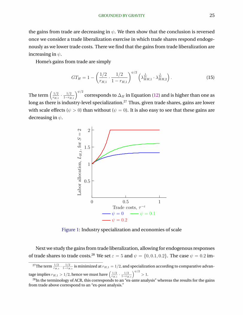
GROUNDED BY GRAVITY 25
the gains from trade are decreasing in ψ. We then show that the conclusion is reversed
once we consider a trade liberalization exercise in which trade shares respond endoge-
nously as we lower trade costs. There we find that the gains from trade liberalization are
increasing in ψ.
Home’s gains from trade are simply
GTH = 1−(
1/2
rH,1· 1/2
1− rH,1
)ψ/2 (λ
12εHH,1 · λ
12εHH,2
). (15)
The term(
1/2rH,1· 1/2
1−rH,1
)ψ/2corresponds to ∆H in Equation (12) and is higher than one as
long as there is industry-level specialization.27 Thus, given trade shares, gains are lower
with scale effects (ψ > 0) than without (ψ = 0). It is also easy to see that these gains are
decreasing in ψ.
0.5
1
1.5
2
Lab
orallocation
,LH,1,forS=
2
0 0.5 1Trade costs, τ−ε
ψ = 0 ψ = 0.1
ψ = 0.2
Figure 1: Industry specialization and economies of scale
Next we study the gains from trade liberalization, allowing for endogenous responses
of trade shares to trade costs.28 We set ε = 5 and ψ = 0, 0.1, 0.2. The case ψ = 0.2 im-
27The term 1/2rH,1· 1/21−rH,1
is minimized at rH,1 = 1/2, and specialization according to comparative advan-
tage implies rH,1 > 1/2, hence we must have(
1/2rH,1· 1/21−rH,1
)ψ/2> 1.
28In the terminology of ACR, this corresponds to an “ex-ante analysis” whereas the results for the gainsfrom trade above correspond to an “ex-post analysis.”

26 KUCHERYAVYY-LYN-RODRıGUEZ-CLARE
0.1
0.2
0.3Gainsfrom
trad
eliberalizationforτ=
1
1 5 10Comparative advantage, S
ψ = 0 ψ = 0.1
ψ = 0.2
(a) Scale economies and comparative advan-tage
0.05
0.1
0.15
0.2
Gainsfrom
trad
eliberalizationforS=
2
0 0.5 1Trade costs, τ−ε
ψ = 0 ψ = 0.1
ψ = 0.2
(b) Scale economies and gravity
Figure 2: Gains from trade liberalization
pliesα = 1, as in the standard multi-industry Krugman or Melitz-Pareto models whereas
the case ψ = 0 corresponds to the standard multi-industry gravity model without scale
economies. Setting ψ = 0.1 allows for an intermediate case with 0 < α < 1. Note that
in all these cases Li,k = 1 for all (i, k) under autarky (i.e., when τ = ∞). As τ falls from
∞, country H specializes in industry 1 and country F specializes in industry 2, but the
extent of specialization will be stronger with ψ = 0.2 than ψ = 0.1, and with ψ = 0.1 than
ψ = 0, as illustrated in Figure 1. Figure 2 shows the implications for the gains from trade
liberalization for each of these three cases. We see that the gains from trade liberaliza-
tion increase with ψ. The intuition is simple: countries gain by specializing according
to comparative advantage, and the concentration of production also allows for a greater
exploitation of scale economies, which, in turn, generates additional efficiency gains.29
4.2.2. Outside Good
The fact that, in the region of uniqueness, countries always gain from trade (relative
to autarky) does not necessarily imply that there are always gains from further trade
29The gains from trade liberalization in Home can be seen as the increase in GTH in (15) as τ falls. Thedecline in τ leads to deeper industry-level specialization, as captured by a higher rH,1, and thus increases(
1/2rH,1· 1/21−rH,1
)ψ/2and lowers GTH . But there is also a change in trade shares, and this decreases λ
12ε
HH,1 ·
λ12ε
HH,2, which more than offsets the previous effect.

GROUNDED BY GRAVITY 27
liberalization. In fact, our model nests the model considered by Venables (1987) and so
we know that a decline in inward trade costs may decrease welfare. To see this more
explicitly, consider a case with two countries and two industries, with ε1 = ∞ > ε2,
ψ1 = 0 < ψ2 ≤ 1/ε2 (so thatα2 ≤ 1), and with no trade costs in industry 1, τ12,1 = τ21,1 = 1.
If we start with an interior equilibrium (i.e., Li,k > 0 for i = 1, 2 and k = 1, 2) then wages
are pinned down by (exogenous) productivities in industry 1 (the outside good), and
— suppressing the industry sub-index — the labor allocation in industry 2 is given by
(L1, L2) that solves
wiLi =∑n
SiLαi (wiτni)
−ε P εnβnwnLn, (16)
for i = 1, 2, with P−εn =∑
j SjLαj (wjτnj)
−ε. The case considered by Venables (1987) en-
tails α = 1, in which case the previous system can be rewritten as a system in (P1, P2),
wi =∑n
Si (wiτni)−ε P ε
nβnwnLn. (17)
It is then easy to see that a decline in τ12 leads to an increase in P1 and a decrease in P2,
exactly as in Venables (1987). Of course, if α = 0 then P−εn =∑
j Sαj (wjτnj)
−ε and so P1
would decrease while there would be no change in P2.
We can understand these results by noting that wn/Pn = S1/εn Lψnλ
−1/εnn . If ψ = 0 then
a decline in inward trade costs decreases the domestic trade share λnn and increases
the real wage. But with ψ > 0 there is an offsetting productivity effect arising from the
decline in Ln. If α = 1 then the net effect is negative.
More generally, we can use Equation (16) to show that ∂Pn/∂τni < 0, as with α = 1,
if and only if α ∈ (ατn, 1], where ατn ∈ (0, 1) is a function of import and export shares in
industry 2 — see Appendix D.2. A similar result holds for the effect of a foreign produc-
tivity increase in industry 2: this lowers welfare (i.e., ∂Pn/∂Si > 0 for n 6= i) if and only if
α ∈ (αSn , 1], where αSn is different from ατn because of additional effects associated with a
productivity increase. We summarize these arguments in the following Proposition.
Proposition 6. AssumeN = K = 2, ε1 =∞ > ε2, ψ1 = 0 < ψ2 ≤ 1/ε2 and τ12,1 = τ21,1 = 1,
and assume that the initial equilibrium is interior (i.e., Li,k > 0 for i = 1, 2 and k = 1, 2).
There exists a threshold ατn ∈ (0, 1) such that country n loses from a small unilateral trade
liberalization in industry 2 if and only if α ∈ (ατn, 1]. Similarly, there exists a threshold
αSn ∈ (0, 1) such that country n loses from a small foreign productivity improvement in
industry 2 if and only if α ∈ (αSn , 1].

28 KUCHERYAVYY-LYN-RODRıGUEZ-CLARE
Proof. See Appendix D.2.
These results generalize the propositions of immiserizing inward trade liberalization
and foreign productivity improvements in (16) in two ways. First, the result holds as long
as scale economies are strong enough, with the threshold for α depending on import
and export shares in the industry with scale economies. Second, and more broadly, the
result is shown to be a manifestation of the more general idea that a shock that pushes
a country to specialize in an industry with weak economies of scale (here the outside
good) may lower the gains from trade.
4.3. Gains from Trade: Numbers Using Data
In this subsection we continue our exploration of the gains from trade using actual data.
Using (12) as our reference point, we follow CR and compute measures of λnn,k, en,k,
and rn,k using data on 31 sectors from the WIOD in 2008.30 We start by assuming a
common trade elasticity of 5 for all industries (i.e., εk = 5 for all k) and consider two
cases for the scale elasticity.31 For the first case we assume a common scale elasticity
across all industries and consider three subcases: (i) no scale economies, ψk = 0 for all
k; (ii) intermediate scale economies, ψk = 0.1 for all k; and (iii) strong scale economies,
ψk = 0.2 for all k. Note that these three subcases correspond to assuming αk = 0 for all
k, αk = 0.5 for all k, and αk = 1 for all k, respectively. For the second case we assume
no scale economies for all non-manufacturing industries and strong scale economies
for all manufacturing industries, i.e., ψk = 0 for all k /∈ M and ψk = 0.2 for all k ∈ M,
where M is the set of manufacturing industries. This case is used below to understand
how specialization in industries with weak or strong scale economies affects the gains
from trade.
Columns 1, 2 and 3 in Table 2 report the gains from trade for the first case with scale
elasticities as in subcases (i), (ii) and (iii), respectively, while column 5 reports the de-
gree of industry specialization as represented by the termDKL(en ‖ rn). Consistent with
Proposition 5, gains from trade decrease as we allow for stronger scale economies, and
this decline is stronger for countries that have a higher degree of industry specializa-
tion. This is illustrated in Figure 3, which plots the gains from trade net of the standard
30Equation (12) ignores trade deficits. As discussed in CR, this implies that our results in this subsectioncapture the change in real income rather than the change in real expenditure caused by shutting downtrade and closing any trade deficits that exist in the data.
31We choose a value of 5 for the trade elasticity as this is a typical value used in the literature — seeHead and Mayer (2014).

GROUNDED BY GRAVITY 29
Figure 3: Degree of specialization and gains from trade
ACR gains (i.e., the gains that would arise in the absence of scale economies) for each
subcase.
Turning to the second case, note that here we have
GTn = 1−
(∏k
(λnn,k)en,k exp
[∑k∈M
en,k ln (en,k/rn,k)
])0.2
.
The term∑
k∈M en,k ln (en,k/rn,k) is no longer the Kullback-Leibler divergence because we
are only adding across k ∈M, so both∑
k∈M en,k and∑
k∈M rn,k can be lower than 1. This
implies that this term can be negative (capturing specialization in manufacturing) and
exert a positive effect on the gains from trade. Column 4 in Table 2 reports the gains from
trade associated with this case, while column 6 reports the term∑
k∈M en,k ln (en,k/rn,k).
As expected, countries that specialize in manufacturing industries have higher gains
from trade than in the case without scale economies. Figure 4 illustrates this by plotting
the pattern of specialization (PS) — measuring in this case the tendency to specialize in
manufacturing — against the the degree of specialization (DS) for selected countries as
defined in (14). For each point we also report the name of the country, the standard ACR
gains and the gains with αk = 1 in all manufacturing industries, respectively.

30 KUCHERYAVYY-LYN-RODRıGUEZ-CLARE
Figure 4: Pattern of specialization and gains from trade
Next, we allow for heterogeneous trade elasticities across industries. Trade elastic-
ities for agriculture and manufacturing industries are from Caliendo and Parro (2015),
while for service industries we assume a trade elasticity of 5.32 For each industry we
maintain the assumption that the scale elasticity is inversely proportional to the trade
elasticity and, consistent with our first exercise, separately consider three cases: (i) ψk =
0 for all k, (ii) ψk = 0.5/εk for all k, and (iii) ψk = 1/εk for all k.
The gains corresponding to these three cases are reported in columns 1, 2 and 3 of
Table 3. While cross-country average gains from trade are not very different across the
three cases, we do see that for some countries the gains can be substantially larger with
economies of scale, while for others these gains are much smaller. For example, relative
to the case with no scale economies, Japan’s gains almost double in the intermediate
case, and almost triple in the case with the highest scale elasticity (to be precise, gains
are 2.4%, 4.3% and 6.1%, respectively), whereas for Greece the reverse is true (gains are
14.5%, 10.1% and 5.5%, respectively). Still for other countries these gains do not change
much. For example, in Austria’s case gains are 29.1%, 29.3% and 29.4%.
To better understand these results, Table 3 reports the DS, PS and overall effect on
32Since there is little trade in services the value of that elasticity has negligible effects.

GROUNDED BY GRAVITY 31
gains (i.e., the term inside the square parenthesis on the RHS of Equation (14)) in columns
4, 5 and 6, respectively. On closer examination we now see that Japan’s tendency to spe-
cialize in industries with higher than average scale economies (PS is positive) is domi-
nant enough to overpower DS, thereby implying larger gains from trade relative to the
standard framework without scale economies. In contrast, for Greece the tendency to
specialize in industries with lower than average scale economies (PS is negative) rein-
forces DS, implying lower gains from trade. Interestingly, while the results also reveal
China’s tendency to specialize in industries with higher than average scale economies
(PS is higher than zero), the extent of this pattern of specialization is not sufficient to im-
ply larger overall gains from trade. Finally, notice that these results generalize insights
from the previous case in which scale economies are assumed only in manufacturing
industries.
4.4. Gains from Trade Liberalization and Foreign Productivity Gains
We now use the exact hat algebra approach popularized by Dekle, Eaton and Kortum
(2008) to explore the implications of a decline in inward trade costs or productivity gains
abroad. This technique works as long as we start from an equilibrium that does not have
corners, which is the case in our data as there are no (i, k) pairs withLi,k = 0. As we show
in Appendix D.3, the system to compute the hat changes in labor allocations and wages
is
Li,k ≥ 0, G′i,k
(w, Lk
)≥ 0, Li,kG
′i,k
(w, Lk
)= 0, for all (i, k),∑
k
Li,kYi,k = Yi, for all i,
where Yi ≡ wiLi and Yi,k ≡ wiLi,k, and
G′i,k
(w, Lk
)≡ wi −
1
Li,kYi,k
∑n
Si,kLαki,k (wiτni,k)
−εk λni,k∑l Sl,kL
αkl,k (wlτnl,k)
−εk λnl,kβn,k(wnYn +Dn),
where Dn are trade imbalances in the data. Note that this still allows the counterfactual
equilibrium to exhibit corner allocations. Therefore, we need to calculate changes in
welfare explicitly by using the formula wn/Pn, where changes in price indices are given

32 KUCHERYAVYY-LYN-RODRıGUEZ-CLARE
by
Pn =∏k
(∑l
Sl,kLαkl,k (wlτnl,k)
−εk λnl,k
)−βn,k/εk.
We use the algorithm outlined in Section 3.3 to compute w and L given some ex-
ogenous shock to trade costs or technology levels. A detailed description of the algo-
rithm is in Appendix D.4. Theoretical results from Section 4.2.2 suggest that there might
be losses from unilateral trade liberalization or foreign productivity improvements. To
explore these theoretical results quantitatively, we again divide all sectors into manu-
facturing (M) and non-manufacturing. We assume that non-manufacturing sectors do
not exhibit economies of scale (αk = 0 for these sectors), while for the manufactur-
ing sectors we consider three possible scenarios: “low” α (αM = 0), “intermediate” α
(αM = 1/2), and “high” α (αM = 1).
In the first three columns of Table 4 we present results of the exercise where a coun-
try unilaterally lowers trade costs with all other countries by 10% in manufacturing in-
dustries. Each row in these columns presents welfare implications of this exercise for
a particular country. For example, the row corresponding to the United States presents
welfare changes for that country given with τni,k = 0.9 for n = US and all k ∈ M and
with all other parameters unchanged. In the last three columns of Table 4 we present
the welfare implications of productivity increase of 1% in all manufacturing sectors in
China, Sik = 1.01εk for i = China and all k ∈M.33
The results in Table 4 reveal that the gains from unilateral trade liberalization in the
sectors with scale economies get smaller as we consider a higher scale elasticity. For
example, the gains for the United States decline from 0.39% when αM = 0 to 0.17% for
αM = 1. Still, in contrast to the results of Section 4.2.2, even for αM = 1 the gains
are positive for all countries. One key difference between the theoretical exercise in
Section 4.2.2 and the quantitative exercise in Table 4 is that in the theoretical exercise
we have an outside good that pins down wages, whereas in the quantitative exercise
wages fully adjust in response to the shock. In Table 5 we considered the same change in
trade costs as in the first three columns of Table 4 but holding wages fixed. As we see in
the last column of Table 5, now Japan and Korea experience losses from unilateral trade
liberalization in manufacturing if αM = 1. To get even closer to the theoretical exercise
33Holding wages fixed, the hat change in the domestic price index of country i in sector k given someSik is S1/εk
i,k . That is why, to think of an x% productivity increase in China’s sector k, we set Si,k = (1 +x)εk .

GROUNDED BY GRAVITY 33
in Section 4.2.2, we aggregated all sectors into manufacturing and non-manufacturing
and all countries into the liberalizing country and the rest of the world. Columns 4-6
of Table 5 report the results associated with a shock τni,M = 0.9, whereas columns 1-3
report those associated with a smaller shock τni,M = 0.99. Column 6 shows that now
most countries lose from unilateral trade liberalization when αM = 1, while in column
3 we see that all countries lose. The reason that some countries still gain in the case of
the larger shock is that the shock pushes them to a corner equilibrium in which they no
longer allocate any labor to manufacturing.
Turning to the gains from foreign productivity improvements in the industries with
scale economies, the last three columns of Table 4 show that some countries lose when
China’s productivity increases in manufacturing. Negative values in column 4 simply re-
flect terms of trade effects, which worsen for countries that compete more directly with
China. Columns 5 and 6 show additional effects arising from the mechanism outlined
in Section 4.2.2. In particular, China’s productivity increase in manufacturing implies a
contraction in manufacturing employment in other countries, which in turn leads to a
decline in productivity given the presence of scale economies in that sector. Thus, we
see more and more countries losing from China’s productivity increase as the strength
of scale economies increases to αM = 1/2 and then to αM = 1.
We explore these findings further in Table 6, where (as in Table 5) we fix wages to
the baseline equilibrium (i.e., wi = 1). With no terms of trade changes, now all coun-
tries gain from China’s productivity increase if there are no scale economies (column 7),
and more and more countries lose as scale economies become stronger. To link these
findings with the theoretical results in Section 4.2.2, the first three columns of Table 6
show analogous results but after aggregating to two sectors (manufacturing and non-
manufacturing) and two countries (the country in each row and the rest of the world).
Columns 1 and 2 show that almost all countries gain from a productivity increase in
manufacturing in the rest of the world if αM ≤ 1/2 but all countries lose when αM = 1, a
reflection of the fact that in most cases the actual threshold αS derived in Section 4.2.2
is high and close to 1. A final set of results is presented in columns 4-6, which show
analogous results to those in columns 1-3 but for a doubling of foreign productivity. In-
terestingly, this now leads to gains in all countries. The reason is that the shock is so
large that manufacturing employment falls to zero in all countries, thus truncating the
mechanism in Section 4.2.2 since a sector cannot keep shrinking after it vanishes.

34 KUCHERYAVYY-LYN-RODRıGUEZ-CLARE
5. Scale Economies and Trade Flows
In this subsection we quantify the role of scale economies in determining industry-level
specialization and trade flows. In particular, we ask how these variables would change
if we shut down scale economies but leave all other exogenous variables unchanged.
We rely on the fact that if L is an equilibrium of the actual economy with scale eco-
nomies then it is also an equilibrium of the economy with no scale economies given
by
wiLi,k =N∑n=1
Ti,k (wiτni,k)−εk∑N
l=1 Tl,k (wlτnl,k)−εk βn,k(wnLn +Dn)
andK∑k=1
Li,k = Li,
where Ti,k ≡ Si,kLαki,k and where Dn are trade deficits satisfying
∑nDn = 0. Thus, if we
want to know the counterfactual allocation for the economy with αk = 0 for all k but
everything else equal, we can use the exact hat algebra approach in the economy with
no scale effects subjected to a shock to productivities Ti,k given by Ti,k = S ′i,k/(Si,kL
αki,k
)=
Si,kL−αki,k .34 To focus on the interaction between specialization and scale economies, we
assume that Si,k is such that if country iwas in autarky then the shock would have no ef-
fect on productivity — since in autarky Li,k = βi,kLi this requires Si,k = (βi,kLi)αk . Using
Li,k = ri,kLi and measuring βi,k by ei,k, this implies that Ti,k = (ei,k/ri,k)αk . Combining
the two previous equations and using Yi ≡ wiLi, we get a system in wage changes given
by
wiYi =K∑k=1
N∑n=1
(ei,k/ri,k)αk (wi)
−εk λni,k∑Nl=1(el,k/rl,k)αk (wl)
−εk λnl,ken,k (wnYn +Dn) .
The solution for wi can then be used to get the implied hat change in the labor allocation
from
Li,k =1
wiYi,k
N∑n=1
(ei,k/ri,k)αk (wi)
−εk λni,k∑Nl=1(el,k/rl,k)αk (wl)
−εk λnl,ken,k (wnYn +Dn) ,
34We can ignore corner solutions because the data has no zeros at the industry level (i.e., ri,k > 0 for alli, k) and the shock that we consider moves us away from corners.

GROUNDED BY GRAVITY 35
where Yi,k ≡ wiLi,k. Finally, we can get the implied change in trade flows from
Xni,k =1
Xni,k
· (ei,k/ri,k)αk (wi)
−εk λni,k∑Nl=1(el,k/rl,k)αk (wl)
−εk λnl,ken,k (wnYn +Dn) .
Table 7 presents the results of this exercise for each of the countries in our sam-
ple. Column 1 reports the degree of specialization (DS) in the data as defined in (13).
Columns 2 and 3 report, respectively, the implied percentage change in DS and in total
exports for each country when αk = 1/2 and εk = 5 for all k. Columns 4 and 5 do the
same but for αk = 1.
As expected, the removal of economies of scale implies a decline in the degree of
specialization and total trade. Column 2 shows that the decline in DS is quite strong
even in the case in which the initial economies of scale are given by αk = 1/2 for all k,
withDS falling by more than 50% in almost all cases. Column 4 shows that this decline is
much sharper in the case of αk = 1 for all k, with DS falling by more than 90% in almost
half of all cases. Columns 3 and 5 show that total exports fall but less dramatically: the
decline in total world exports corresponding to these two columns is 5.4% and 10%.
These results imply that if the data is generated by a gravity model with scale eco-
nomies as strong as in the Krugman model (i.e., αk = 1 for all k), then most of the
industry-level specialization that we observe is due to scale economies rather than Ri-
cardian comparative advantage. In other words, without scale economies amplifying Ri-
cardian productivity differences, industry-level specialization would be, in many cases,
more than 90% less than what we see in the data. In contrast, since most of world trade
is intra-industry trade, scale economies as strong as in the Krugman model would be
responsible for only around 10% of total world trade.
6. Concluding Remarks
For over a century since Alfred Marshall’s initial exposition, economists have been in-
trigued with the implications of industry-level external economies of scale for trading
economies. Despite such interest, however, the discomfort with the plethora of equilib-
ria and counter-intuitive implications in early work relegated Marshallian externalities
to the “back-burner” of the recent trade literature. In this paper we show how one can
add Marshallian externalities to the Eaton and Kortum (2002) framework while retain-
ing the property that the equilibrium is unique. The resulting model has exactly the

36 KUCHERYAVYY-LYN-RODRıGUEZ-CLARE
same mathematical structure as generalized versions of the multi-industry Krugman
and Melitz-Pareto models and so our uniqueness result applies to these well-known
models as well. The key condition for uniqueness is simple and intuitive: the scale elas-
ticity must be weakly lower than the inverse of the trade elasticity for all industries.
Remarkably, if parameters are in the region of uniqueness then all countries gain
from trade. Economies of scale tend to make gains from trade lower relative to models
without scale economies, although the opposite may happen for countries that hap-
pen to specialize in industries with stronger than average scale economies. In turn, the
welfare effects of unilateral trade liberalization are more subtle than in gravity models
without scale economies: beyond standard terms of trade effects, the reallocation of
labor caused by changes in trade costs lead to endogenous productivity changes with
additional welfare implications.
Finally, our exploration of the role of economies of scale in explaining trade flows and
industry-level specialization in the data yields very definitive results: if scale economies
are as strong as those in the Krugman model then most of the industry-level special-
ization that we see in the data is due to economies of scale rather than pure Ricardian
comparative advantage.
Many questions remain open for future research. How can we extend our unique-
ness results for endogenous wages beyond the cases of N = 2, or frictionless trade?
How can we robustly estimate the strength of industry-level scale economies? Is the
condition necessary for uniqueness likely to be satisfied? Are scale economies stronger
in some industries than others? If so, which ones? How does the presence of industry-
level scale economies affect country-level and world-level optimal trade policies?

GROUNDED BY GRAVITY 37
Table 2: Gains from Trade, Common Elasticities
Gains from TradeDegree of
specialization
ψk = 0
commonψk = 0.1
commonψk = 0.2
commonψk = 0.2
manuf.All
industriesManuf.
only
Country (1) (2) (3) (4) (5) (6)
AUS 3.0% 2.7% 2.3% 2.1% 0.036 0.048AUT 8.7% 8.6% 8.5% 9.0% 0.015 -0.012BEL 13.8% 13.2% 12.5% 14.0% 0.072 -0.012BRA 1.6% 1.6% 1.5% 1.5% 0.004 0.004CAN 5.2% 5.0% 4.7% 4.5% 0.024 0.037CHN 3.0% 2.8% 2.7% 3.5% 0.016 -0.025CZE 8.0% 7.8% 7.7% 8.4% 0.014 -0.022DEU 6.0% 5.7% 5.4% 6.9% 0.033 -0.046DNK 9.5% 8.6% 7.8% 9.3% 0.090 0.009ESP 4.1% 3.8% 3.6% 3.8% 0.023 0.011FIN 5.5% 5.1% 4.8% 6.3% 0.036 -0.042FRA 4.0% 3.8% 3.7% 4.2% 0.020 -0.006GBR 4.6% 4.5% 4.5% 4.2% 0.008 0.022GRC 5.7% 4.6% 3.6% 3.5% 0.110 0.114HUN 12.3% 12.0% 11.8% 11.9% 0.027 0.018IDN 3.5% 3.4% 3.3% 3.2% 0.013 0.018IND 3.1% 3.0% 2.9% 2.8% 0.013 0.014IRL 10.1% 9.5% 8.8% 10.6% 0.069 -0.027ITA 3.7% 3.4% 3.2% 3.9% 0.026 -0.015JPN 2.4% 2.0% 1.6% 2.9% 0.041 -0.023KOR 6.6% 5.3% 4.1% 7.3% 0.133 -0.037MEX 4.5% 4.3% 4.1% 3.8% 0.018 0.038NLD 9.4% 9.3% 9.1% 9.8% 0.020 -0.018POL 6.0% 5.9% 5.8% 5.9% 0.009 0.006PRT 6.3% 6.0% 5.7% 5.7% 0.032 0.032ROM 6.2% 6.0% 5.8% 5.1% 0.020 0.059RUS 3.2% 2.5% 1.7% 0.8% 0.076 0.123SVK 11.5% 11.2% 10.9% 11.7% 0.038 -0.011SVN 13.3% 12.3% 11.3% 13.4% 0.112 -0.008SWE 6.7% 6.5% 6.4% 7.2% 0.019 -0.026TUR 4.0% 3.9% 3.7% 4.1% 0.018 -0.004TWN 9.6% 8.6% 7.5% 10.2% 0.112 -0.036USA 2.1% 2.0% 1.9% 1.7% 0.007 0.020RoW 6.9% 6.4% 6.0% 5.8% 0.050 0.061
Average 6.3% 5.9% 5.6% 6.1% 0.040 0.008

38 KUCHERYAVYY-LYN-RODRıGUEZ-CLARE
Table 3: Gains from Trade, Caliendo-Parro elasticities
Gains from TradeDegree and Pattern
of Specialization
ψk = 0 ψk = 0.5εk
ψk = 1εk
DS PS Overall
Country (1) (2) (3) (4) (5) (6)
AUS 7.6% 5.5% 3.5% 0.036 -0.111 0.147AUT 29.1% 29.3% 29.4% 0.015 0.027 -0.012BEL 29.8% 29.6% 29.3% 0.072 0.051 0.021BRA 3.4% 3.6% 3.9% 0.004 0.019 -0.015CAN 16.7% 15.7% 14.7% 0.024 -0.056 0.081CHN 4.1% 4.0% 4.0% 0.016 0.013 0.003CZE 16.6% 18.4% 20.2% 0.014 0.166 -0.151DEU 12.9% 15.1% 17.2% 0.033 0.204 -0.171DNK 24.6% 22.4% 20.1% 0.090 -0.104 0.194ESP 9.4% 9.7% 10.0% 0.023 0.047 -0.025FIN 10.3% 9.9% 9.5% 0.036 0.007 0.029FRA 9.8% 10.5% 11.3% 0.020 0.076 -0.056GBR 11.7% 11.4% 11.1% 0.008 -0.018 0.025GRC 14.5% 10.1% 5.5% 0.110 -0.230 0.340HUN 31.1% 31.9% 32.7% 0.027 0.103 -0.076IDN 6.3% 5.3% 4.3% 0.013 -0.058 0.070IND 4.6% 4.5% 4.4% 0.013 0.006 0.008IRL 18.3% 15.4% 12.5% 0.069 -0.163 0.232ITA 8.3% 8.4% 8.5% 0.026 0.036 -0.010JPN 2.4% 4.3% 6.1% 0.041 0.173 -0.133KOR 6.2% 8.7% 11.2% 0.133 0.318 -0.185MEX 11.5% 12.0% 12.5% 0.018 0.057 -0.039NLD 22.7% 22.0% 21.2% 0.020 -0.044 0.064POL 18.0% 18.6% 19.3% 0.009 0.064 -0.055PRT 19.0% 18.1% 17.1% 0.032 -0.050 0.081ROM 13.8% 12.4% 11.0% 0.020 -0.089 0.110RUS 15.9% 9.0% 1.6% 0.076 -0.457 0.534SVK 30.3% 31.7% 33.1% 0.038 0.176 -0.138SVN 33.1% 33.2% 33.3% 0.112 0.120 -0.008SWE 13.7% 14.5% 15.4% 0.019 0.084 -0.065TUR 11.3% 11.9% 12.5% 0.018 0.064 -0.047TWN 10.2% 9.8% 9.5% 0.112 0.084 0.028USA 4.5% 4.4% 4.3% 0.007 0.000 0.007RoW 14.8% 11.1% 7.2% 0.050 -0.241 0.290
Average 14.6% 14.2% 13.7% 0.040 0.008 0.032

GROUNDED BY GRAVITY 39
Table 4: Inward Trade Liberalization and Foreign Productivity Improvement
τni,k = 0.9 ∀ k ∈M SCHN,k = 1.01εk ∀ k ∈M
αM = 0 αM = 0.5 αM = 1 αM = 0 αM = 0.5 αM = 1
Country (1) (2) (3) (4)* (5)* (6)*
AUS 0.64% 0.51% 0.25% 0.94% 0.31% -0.76%AUT 1.61% 1.51% 0.96% 0.19% -0.15% -0.25%BEL 1.89% 1.81% 1.45% 0.16% -0.11% -0.44%BRA 0.35% 0.26% 0.16% 0.32% 0.10% -0.13%CAN 1.18% 1.05% 0.69% 0.50% 0.13% -0.28%CHN 0.63% 0.54% 0.43% 48.87% 50.99% 53.08%CZE 1.85% 1.76% 1.50% 0.28% 0.18% 0.32%DEU 1.26% 1.18% 0.83% 0.08% -0.11% -0.27%DNK 1.32% 1.21% 0.82% 0.37% -0.05% -0.58%ESP 0.70% 0.59% 0.43% 0.03% -0.21% -0.47%FIN 0.98% 0.89% 0.76% -0.11% -0.29% -0.28%FRA 0.82% 0.74% 0.64% 0.08% -0.09% -0.21%GBR 0.85% 0.75% 0.58% 0.24% 0.02% -0.18%GRC 0.90% 0.64% 0.08% 0.62% 0.27% -0.22%HUN 2.48% 2.35% 1.91% 0.36% 0.15% 0.01%IDN 0.77% 0.64% 0.48% 0.52% 0.09% -0.19%IND 0.61% 0.50% 0.28% 0.35% 0.15% 0.13%IRL 1.19% 1.06% 0.74% -0.20% -0.50% -0.66%ITA 0.69% 0.61% 0.53% -0.04% -0.18% -0.21%JPN 0.30% 0.25% 0.20% 0.00% -0.15% -0.17%KOR 0.80% 0.68% 0.53% -0.00% -0.55% -0.97%MEX 1.12% 1.00% 0.73% 0.39% 0.29% 0.26%NLD 1.32% 1.22% 0.80% 0.10% -0.27% -0.86%POL 1.31% 1.22% 0.87% 0.33% 0.17% 0.04%PRT 1.14% 1.00% 0.61% 0.31% -0.04% -0.39%ROM 1.27% 1.11% 0.81% 0.15% -0.10% -0.24%RUS 0.87% 0.65% 0.24% 0.70% 0.31% -0.24%SVK 2.31% 2.22% 1.72% 0.12% -0.03% -0.13%SVN 2.11% 2.01% 1.41% 0.08% -0.08% -0.27%SWE 1.22% 1.11% 0.81% -0.09% -0.48% -0.81%TUR 0.73% 0.65% 0.27% 0.05% -0.02% -0.05%TWN 1.66% 1.51% 0.73% -0.13% -0.29% -0.70%USA 0.39% 0.30% 0.17% 0.28% 0.05% -0.17%RoW 1.14% 0.93% 0.56% 0.90% 0.14% -1.12%
* The numbers specified in the column have been multiplied by 100.

40 KUCHERYAVYY-LYN-RODRıGUEZ-CLARE
Table 5: Unilateral Trade Liberalization with Fixed Wages
τni,k = 0.99 ∀ k ∈M τni,k = 0.9 ∀ k ∈M
2× 2 N × S
αM = 0 αM = 0.5 αM = 1 αM = 0 αM = 0.5 αM = 1 αM = 0 αM = 0.5 αM = 1
Country (1) (2) (3) (4) (5) (6) (7) (8) (9)
AUS 0.08% 0.05% -0.00% 0.91% 0.69% -0.00% 0.89% 0.71% 0.22%AUT 0.17% 0.15% -0.00% 1.97% 1.82% 0.31% 1.94% 1.81% 1.12%BEL 0.19% 0.18% -0.01% 2.12% 2.08% 1.44% 2.10% 2.05% 1.75%BRA 0.05% 0.03% -0.00% 0.60% 0.36% -0.00% 0.59% 0.38% 0.03%CAN 0.13% 0.11% -0.00% 1.54% 1.32% -0.03% 1.51% 1.34% 0.68%CHN 0.08% 0.05% -0.01% 1.04% 0.68% -0.09% 1.01% 0.79% 0.91%CZE 0.21% 0.18% -0.00% 2.39% 2.15% -0.03% 2.36% 2.15% 1.05%DEU 0.14% 0.12% -0.01% 1.71% 1.50% -0.18% 1.69% 1.54% 1.51%DNK 0.14% 0.13% -0.00% 1.56% 1.48% 0.62% 1.55% 1.46% 0.90%ESP 0.09% 0.06% -0.00% 1.13% 0.85% -0.01% 1.10% 0.89% 0.24%FIN 0.11% 0.09% -0.00% 1.36% 1.13% -0.01% 1.33% 1.14% 0.22%FRA 0.10% 0.08% -0.00% 1.18% 0.98% -0.04% 1.17% 1.01% 0.74%GBR 0.09% 0.08% -0.00% 1.10% 0.96% -0.03% 1.08% 0.97% 0.68%GRC 0.12% 0.08% -0.00% 1.40% 1.08% -0.00% 1.37% 1.12% 0.51%HUN 0.26% 0.24% -0.00% 2.93% 2.79% 1.27% 2.89% 2.73% 2.07%IDN 0.09% 0.06% -0.00% 1.16% 0.80% -0.00% 1.11% 0.86% 0.50%IND 0.08% 0.05% -0.00% 1.01% 0.67% -0.01% 0.97% 0.73% 0.49%IRL 0.13% 0.11% -0.00% 1.50% 1.39% -0.01% 1.49% 1.37% 0.77%ITA 0.09% 0.06% -0.00% 1.10% 0.82% -0.03% 1.09% 0.86% 0.21%JPN 0.04% 0.03% -0.00% 0.55% 0.35% -0.02% 0.54% 0.36% -0.01%KOR 0.11% 0.07% -0.00% 1.35% 0.97% -0.02% 1.34% 0.98% -0.06%MEX 0.13% 0.10% -0.00% 1.61% 1.26% -0.02% 1.56% 1.31% 0.37%NLD 0.14% 0.13% -0.00% 1.54% 1.47% 0.66% 1.52% 1.45% 1.11%POL 0.15% 0.12% -0.00% 1.77% 1.50% -0.02% 1.71% 1.53% 0.80%PRT 0.14% 0.11% -0.00% 1.60% 1.36% -0.01% 1.57% 1.38% 0.52%ROM 0.15% 0.11% -0.00% 1.82% 1.47% -0.00% 1.76% 1.53% 1.10%RUS 0.10% 0.06% -0.00% 1.23% 0.84% -0.00% 1.17% 0.90% 0.66%SVK 0.24% 0.23% -0.00% 2.75% 2.63% 1.23% 2.73% 2.60% 1.71%SVN 0.23% 0.21% -0.00% 2.55% 2.42% 1.08% 2.52% 2.38% 1.40%SWE 0.13% 0.11% -0.00% 1.58% 1.40% -0.02% 1.55% 1.40% 0.90%TUR 0.09% 0.06% -0.00% 1.14% 0.81% -0.01% 1.07% 0.88% 0.47%TWN 0.19% 0.16% -0.00% 2.22% 1.95% -0.04% 2.17% 1.88% 0.94%USA 0.06% 0.04% -0.00% 0.70% 0.48% -0.04% 0.68% 0.55% 0.47%RoW 0.14% 0.11% -0.01% 1.64% 1.40% -0.20% 1.61% 1.43% 1.11%

GROUNDED BY GRAVITY 41
Table 6: Foreign Productivity Improvement with Fixed Wages
SRoW,k = 1.01εk ∀ k ∈M SRoW,k = 2εk ∀ k ∈M SCHN,k = 1.01εk ∀ k ∈M
2× 2 N × S
αM = 0 αM = 0.5 αM = 1 αM = 0 αM = 0.5 αM = 1 αM = 0 αM = 0.5 αM = 1
Country (1)* (2)* (3)* (4) (5) (6) (7)* (8)* (9)*
AUS 7.47% 3.05% -7.11% 10.31% 10.14% 10.15% 1.66% 1.13% -0.62%AUT 16.99% 9.50% -47.78% 17.80% 17.70% 17.72% 0.79% -0.25% 0.61%BEL 18.97% 14.73% -85.11% 16.81% 16.79% 16.81% 1.05% 0.30% -3.95%BRA 4.61% 0.46% -5.33% 11.09% 10.27% 10.15% 0.88% 0.36% 0.25%CAN 12.96% 6.23% -21.34% 15.10% 14.99% 15.03% 1.86% 1.31% -2.77%CHN 8.02% -0.67% -16.28% 19.14% 18.96% 20.14% 40.93% 47.40% 74.24%CZE 20.30% 9.64% -51.27% 23.36% 23.18% 23.20% 2.46% 1.80% 7.75%DEU 14.26% 5.27% -40.92% 17.89% 17.92% 18.17% 1.56% 0.61% -3.74%DNK 13.71% 8.82% -43.30% 13.16% 13.11% 13.11% 0.97% 0.23% 1.52%ESP 9.17% 3.06% -11.18% 13.45% 13.23% 13.27% 0.94% 0.43% 0.26%FIN 11.19% 2.38% -28.54% 15.34% 15.08% 15.09% 1.28% 0.36% -0.16%FRA 9.82% 3.56% -18.07% 12.62% 12.52% 12.60% 0.86% 0.29% 0.62%GBR 9.38% 4.83% -16.24% 10.33% 10.28% 10.31% 1.05% 0.63% 0.33%GRC 11.74% 6.95% -4.39% 14.25% 14.09% 14.09% 0.87% 0.28% 0.48%HUN 25.66% 17.03% -76.88% 25.62% 25.52% 25.53% 2.46% 1.62% 16.01%IDN 9.17% 2.00% -11.34% 16.20% 15.66% 15.64% 2.23% 1.19% -0.22%IND 7.97% 1.93% -8.05% 15.21% 14.64% 14.65% 2.00% 1.40% 3.22%IRL 12.83% 5.61% -46.63% 14.15% 14.04% 14.05% 1.39% 0.54% 1.87%ITA 8.85% 1.69% -15.11% 14.18% 13.91% 14.01% 0.77% -0.04% 0.13%JPN 4.22% -0.68% -8.31% 10.38% 9.75% 9.87% 1.48% 0.25% -3.19%KOR 10.66% 0.46% -20.93% 19.66% 19.05% 19.13% 3.45% 0.74% -11.19%MEX 13.24% 5.02% -16.90% 18.32% 18.06% 18.11% 2.12% 1.62% -1.57%NLD 13.52% 8.79% -52.95% 12.88% 12.84% 12.86% 1.27% 0.88% -0.41%POL 14.78% 6.18% -27.07% 18.17% 17.99% 18.01% 1.63% 1.14% 0.54%PRT 13.55% 6.66% -19.55% 15.77% 15.62% 15.62% 0.43% -0.37% 0.96%ROM 15.19% 7.30% -15.50% 19.18% 18.95% 18.95% 0.80% 0.00% 2.79%RUS 9.90% 4.71% -4.31% 15.60% 15.26% 15.29% 1.66% 1.06% 0.02%SVK 24.11% 16.06% -80.89% 23.77% 23.67% 23.68% 1.85% 0.70% -5.44%SVN 22.32% 14.67% -69.27% 22.01% 21.91% 21.91% 1.29% 0.27% 11.58%SWE 13.29% 5.41% -35.17% 15.54% 15.40% 15.42% 0.70% -0.32% 1.25%TUR 9.08% 1.96% -12.45% 15.21% 14.79% 14.79% 1.23% 0.53% 1.84%TWN 18.58% 6.98% -50.21% 22.95% 22.74% 22.78% 3.93% 1.15% -21.74%USA 5.53% 1.98% -4.81% 9.36% 9.37% 9.68% 1.36% 0.86% -0.02%RoW 13.79% 7.49% -18.09% 16.65% 16.83% 17.20% 3.01% 2.17% -7.27%
* The numbers specified in the column have been multiplied by 100.

42 KUCHERYAVYY-LYN-RODRıGUEZ-CLARE
Table 7: Scale and Trade Flows
α = 0.5 α = 1
DSi DSi EX i DSi EX i
Country (1) (2) (3) (4) (5)
AUS 0.04 -60.80% -9.44% -93.03% -16.61%AUT 0.02 -61.85% -0.85% -83.99% -1.38%BEL 0.07 -64.83% -0.86% -98.20% -0.36%BRA 0.00 -27.81% -3.99% -49.37% -7.73%CAN 0.02 -62.92% -1.84% -93.10% -2.57%CHN 0.02 -50.09% -5.71% -77.27% -10.19%CZE 0.01 -64.56% -2.24% -89.40% -4.07%DEU 0.03 -57.46% -3.45% -86.77% -6.47%DNK 0.09 -72.81% -7.52% -96.89% -10.50%ESP 0.02 -65.03% -2.08% -92.65% -3.93%FIN 0.04 -56.97% -5.17% -84.00% -9.23%FRA 0.02 -65.84% -2.65% -94.39% -5.50%GBR 0.01 -52.64% -2.09% -80.93% -3.93%GRC 0.11 -80.81% -34.11% -92.28% -36.71%HUN 0.03 -61.97% -2.43% -86.21% -4.16%IDN 0.01 -39.76% -3.14% -73.45% -7.05%IND 0.01 -56.57% -3.09% -78.23% -4.30%IRL 0.07 -62.27% -4.05% -92.27% -6.43%ITA 0.03 -67.40% -3.66% -95.44% -6.92%JPN 0.04 -64.05% -7.84% -91.77% -16.35%KOR 0.13 -64.98% -7.19% -94.25% -17.12%MEX 0.02 -47.52% -3.45% -75.86% -6.32%NLD 0.02 -58.22% -2.80% -84.96% -5.20%POL 0.01 -64.82% -2.10% -89.59% -3.65%PRT 0.03 -64.28% -1.68% -90.12% -2.58%ROM 0.02 -50.04% -1.92% -74.73% -2.60%RUS 0.08 -50.66% -13.67% -79.56% -25.18%SVK 0.04 -68.64% -2.56% -95.38% -4.71%SVN 0.11 -59.87% -1.38% -97.67% -0.71%SWE 0.02 -56.61% -2.67% -85.26% -5.07%TUR 0.02 -56.67% -7.46% -81.44% -13.15%TWN 0.11 -64.59% -8.37% -93.34% -16.58%USA 0.01 -47.24% -4.85% -71.86% -8.63%RoW 0.05 -53.75% -7.86% -84.78% -15.04%

GROUNDED BY GRAVITY 43
A. Definitions
It is clear that both functions Gi,k (w,Lk) and Li,kGi,k (w,Lk) which appear in the non-
linear complementarity problem (3) are well-defined for all positive wages and positive
labor allocations, i.e., for all w ∈ RN++ and Lk ∈ RN
++. We are interested in extending
the definitions of Gi,k (w,Lk) and Li,kGi,k (w,Lk) to the set of all non-negative labor al-
locations excluding the point with Li,k = 0 for all i, i.e., to the set RN+ \ 0. To this
end, we allow for function Gi,k (w,Lk) to take infinite values. Formally, we consider the
function Gi,k : RN++ × RN
+ \ 0 → R ∪ −∞,+∞,35 and for each given vector of wages
w ∈ RN++ and vector of labor allocations Lk ∈ RN
+ \ 0 we formally define Gi,k (w,Lk)
and Li,kGi,k (w,Lk) by the limits
Gi,k (w,Lk) ≡ limxt→Lk
[wi −
1
xti
∑n
λni,k(w,xt)βn,kwnLn
]
and
Li,kGi,k (w,Lk) ≡ limxt→Lk
xti
[wi −
1
xti
∑n
λni,k(w,xt)βn,kwnLn
],
where xt∞t=1 is any sequence converging to Lk such that xt ∈ RN++ for t = 1, 2, . . . .
Let us verify that functionsGi,k (w,Lk) andLi,kGi,k (w,Lk) are well-defined. Since for
all Lk ∈ RN++ functionsGi,k (w,Lk) and Li,kGi,k (w,Lk) are well-defined and continuous,
the above limits coincide with the values of these functions in the corresponding points.
Next, consider any sequence xt∞t=1 with xt ∈ RN++ for t = 1, 2, . . . and converging to
Lk. We have
limxt→Lk
1
xti
∑n
λni,k(w,xt) = lim
xt→Lk
[xti]αk−1
∑n
Si,k (wiτni,k)−εk∑
l Sl,k [xtl ]αk (wlτnl,k)
−εk βn,kwnLn.
Then, since, Lk 6= 0,
limxt→Lk
∑l
Sl,k[xtl]αk (wlτnl,k)
−εk =∑l
Sl,kLαkl,k (wlτnl,k)
−εk > 0 for all n.
35Here the set R ∪ −∞,+∞ is the extended real number system with symbols−∞ and +∞ followingthe standard conventions (see, for example, p. 11-12 in Rudin, 1976). In particular, for any x ∈ R, −∞ <x < +∞.
44 KUCHERYAVYY-LYN-RODRıGUEZ-CLARE
Hence, limxt→Lk
1
xti
∑n λni,k(w,x
t) =∞ if Li,k = 0 and 0 ≤ αk < 1, and
limxt→Lk
1
xti
∑n λni,k(w,x
t) is a positive number if Li,k > 0 or if αk ≥ 1. This, in turn,
implies that
Gi,k (w,Lk) = limxt→Lk
[wi −
1
xti
∑n
λni,k(w,xt)βn,kwnLn
]
=
−∞, if Li,k = 0 and 0 ≤ αk < 1,
finite number, if Li,k > 0 or αk ≥ 1.
So, the limit always exists and is either −∞ or a finite number. Hence, function Gi,k is
well-defined with its codomain given by the extended real line R ∪ −∞,+∞.
Similarly, it is easy to verify that limxt→Lk xti
[wi −
1
xti
∑n λni,k(w,x
t)βn,kwnLn
]always
exists. Moreover, this limit is always a finite number. Hence, function Li,kGi,k is also
well-defined.
B. Linking Melitz and Marshall
We consider a generalized Melitz-Pareto framework, in which the elasticity of substi-
tution between varieties from different countries, ηk, is different from the elasticity of
substitution between varieties from the same country, σk.
Let us ignore the industry subscript for a moment. Let Ωni denote the set of varieties
that i sells to n. The price index of these goods is Pni ≡(∫
ω∈Ωnipni(ω)1−σdω
) 11−σ
. Let Mi
denote total entry in country i and ϕ∗ni denote the cutoff productivity such that i exports
to n all goods with productivity higher than ϕ∗ni. We have
P 1−σni = Mi
∫ ∞ϕ∗ni
[pni(ϕ)]1−σ dGi(ψ)
= θbθiMi
[σ
σ − 1wiτni
]1−σ ∫ ∞ϕ∗ni
ϕσ−θ−2dϕ
= Mi
[σ
σ − 1wiτni
]1−σbθi (ϕ∗ni)
σ−θ−1
θ − (σ − 1).

GROUNDED BY GRAVITY 45
The condition that determines the cutoff ϕ∗ni is
1
σ
(σ
σ − 1· wiτniϕ∗ni
)1−σP σ−1ni
(PniPn
)1−ηXn = wnfn.
This implies that
ϕ∗ni =wiτniPni
(σ
σ· wnfnXn
) 1σ−1(PniPn
) 1−η1−σ
,
where σ ≡(
σσ−1
)1−σ. Plugging this expression into the expression for the price index
yields
Pni = wiτni
(wiτniPni
(Xn
wnfn
) 11−σ(PniPn
) 1−η1−σ) θ
σ−1−1
M1
1−σi κoi,k,
where
κoi,k ≡σ
σ − 1
bθi[σσ
]1− θσ−1
θ − (σ − 1)
1
1−σ
.
Bringing back the k subindex and using the well known result that in this model equi-
librium entry in each industry must satisfy Mi,k = σk−1σkθk
Li,kFi,k
, we then have
Pni,k = wiτni,k
(wiτni,kPni,k
(Xn,k
wnfn
) 11−σk
(Pni,kPn,k
) 1−ηk1−σk
) θkσk−1
−1
L1
1−σki,k κoi,k.
where κoi,k ≡(σk−1σkθk
F−1i,k
) 11−σk κoi,k. Using Xn,k = βn,kwnLn we get
Pni,k = wiτni,k
(wiτni,kPni,k
(Pni,kPn,k
) 1−ηk1−σk
) θkσk−1
−1
L1
1−σki,k κdn,kκ
oi,k,
where
κdn,k ≡[βn,kLnfn,k
] 11−σk
(θk
σk−1−1
).
Solving for Pni,k we get
P 1−ηkni,k =
[(wiτni,k)
−θk P1−ηk1−σk
(θk−σk+1)
n,k Li,k(κdn,kκ
oi,k)
1−σk]ξk
.
46 KUCHERYAVYY-LYN-RODRıGUEZ-CLARE
where ξk is as defined in the text. Using P 1−ηkn,k =
∑i P
1−ηkni,k and λni,k =
(Pni,kPn,k
)1−ηkwet get
the expression for trade shares in the text. Finally, the expression for the price index in
the text is obtained by combining P 1−ηkn,k =
∑i P
1−ηkni,k with the result above for Pni,k, with
µMelk ≡
(σk−1σk
)σkθk
1θk
(σkσk
)1− θkσk−1
θk−(σk−1)
1θk
.
C. Existence and Uniqueness
C.1. Proof of Proposition 1
Proof of Lemma 1. Here we prove that function F (·) defined in (7) is strictly convex on
Γ. The uniqueness of solution of the minimization problem minx∈Γ F (x) then follows
from the fact that Γ is a convex set, and a strictly convex function can have at most one
global minimum on a convex set.
If 0 < α < 1, then for any n function∑
i anixαi is a strictly concave function. And
since the logarithm is a strictly concave function, F (·) is strictly convex.
If α = 1, then we need to make sure that for any two vectors x 6= y we cannot
have that∑
i anixi =∑
i aniyi for all n. Otherwise, we would have F (γx + (1− γ)y) =
γF (x) + (1 − γ)F (y) for any γ ∈ [0, 1] and strict convexity would be violated. Assump-
tion 1 guarantees that matrix A = (ani) is non-singular. Hence, for any x 6= y we have∑i anixi 6=
∑i aniyi for at least one n. Hence, in case of α = 1, F (·) is also strictly convex
under Assumption 1.
Proof of Lemma 2. Suppose, without loss of generality, that x∗1 = 0. Since∑
n x∗n =∑
n bn > 0, we can also suppose without loss of generality that x∗2 6= 0. Consider the
vector x(ε) = (ε, x∗2 − ε, x∗3, . . . , x∗N), where ε ∈ [0, x∗2]. Clearly, x(ε) ∈ Γ. Define
F (ε) ≡ F (x (ε)) = α∑n
x∗n −∑n
bn ln
(an1ε
α + an2(x∗2 − ε)α +N∑i=2
ani (x∗i )α
).
We now show that F (ε) < F (0) for small enough ε > 0. We have
∂ (aj1εα + aj2(x∗2 − ε)α)
∂ε= αaj1ε
α−1 − αaj2(x∗2 − ε)α−1,

GROUNDED BY GRAVITY 47
which, given α ∈ (0, 1), is positive for small enough ε. This implies that aj1εα + aj2(x∗2 −ε)α +
∑Ni=2 aji [x
∗i ]α > aj2 [x∗2]α +
∑Ni=2 ai [x
∗i ]α for small enough ε. Since ln(·) is a strictly
increasing function, we then get that F (ε) < F (0) for small enough ε, a contradiction.
This implies that x∗ cannot be a global minimum of F (·) on Γ. Hence, in the case of
α ∈ (0, 1) we must have x∗i > 0 for all i.
Proof of Lemma 3. Let us start with the simpler case of α = 1. We can take the set
D ≡x ∈ RN |
∑i anixi > 0 for all n
as the domain of F (·) and use Γ as the constraint
set. Clearly, Γ ⊂ D ∩x ∈ RN |
∑i xi =
∑i bi
and F (·) is differentiable on D for α = 1.
Consider the minimization problem
minx∈D
F (x)
s.t.
xi ≥ 0, i = 1, . . . , N ;∑i
xi =∑i
bi.
(18)
Its first-order conditions, after some manipulations, can be written as
xi ≥ 0,∂F (x)
∂xi≥ 0, xi
∂F (x)
∂xi= 0, i = 1, . . . , N,∑
i
xi =∑i
bi.
These conditions are also sufficient, because F (·) is strictly convex and the set that sat-
isfies the constraints of the minimization problem is a convex set. Then, since Gi (x) =∂F (x)
∂xi, we get that any solution of the minimization problem (18) is also a solution of
the NCP in (6) and vice versa.
Let us now turn to the case with 0 < α < 1. Let x∗ be a minimum of F (·) on Γ.
By Lemma 2, x∗i > 0 for all i. Let δ > 0 be some number such that δ ≤ x∗i for all i =
1, . . . , N . Define the domain of F by D ≡x ∈ RN |xi > δ/2, i = 1, . . . , N
. Consider the
minimization problem:minx∈D
F (x)
s.t.∑i
xi =∑i
bi.
(19)

48 KUCHERYAVYY-LYN-RODRıGUEZ-CLARE
Since D ∩x ∈ RN |
∑i xi =
∑i bi⊂ Γ, if x∗ minimizes F on Γ, it also solves the min-
imization problem (19). Since x∗i > δ/2 for all i, the first-order conditions for (19) are
given by∂F (x∗)
∂xi= 0, i = 1, . . . , N, and
∑i
x∗i =∑i
bi. (20)
Hence, x∗ solves NCP in (6). Conversely, if x∗ solves NCP, then x∗i > 0 for all i because
the condition Gi (x∗) ≥ 0 cannot be satisfied for x∗i = 0 if 0 < α < 1. Hence, x∗ satisfies
conditions (20), which are the first order conditions for an interior solution of (19) with
an appropriately chosen δ > 0. Since these first-order conditions are also sufficient,
x∗ solves (19). Now, suppose by contradiction that the minimum of F (·) on Γ is some
x∗∗ 6= x∗. Then, by Lemma 2, x∗∗i > 0 for all i. Therefore we can extend the open set on
which F (·) is differentiable to include both x∗ and x∗∗. Then both x∗ and x∗∗ satisfy the
first-order conditions (20), which gives a contradiction given that F (·) is strictly convex
and the constraint set is convex. Hence, x∗ is the minimum of F (·) on Γ.
Proof of Lemma 4. Let us formally bring argument α into the notation of function F
defined in (7), i.e., consider the function F (x;α). Lemma 1 establishes that under As-
sumption 1 the solution to the optimization problem minx∈Γ F (x;α) defines a function
x : (0, 1]→ RN+ \ 0. Clearly, F (x;α) is continuous for all x ∈ RN
+ \ 0 and α ∈ (0, 1]. Γ
is a compact set which is the same for all α ∈ (0, 1]. Thus, all conditions for Theorem of
the Maximum (Theorem 3.6) from Stokey, Lucas and Prescott (1989) are statisfied, and
x(α) is continuous for all α ∈ (0, 1].
C.2. Proof of Proposition 2
Proof of Lemma 5. The case with αk = 0 is trivial because labor allocations are ex-
plicitly obtained from the goods market clearing conditions Li,kGi,k (w,Lk) = 0, and the
resulting expression for Li,k(w) are obviously continuous. Below we focus on the case
with αk ∈ (0, 1].
Define a multi-valued correspondence Γk : RN++ → RN
+ \ 0 by
Γk (w) =
Lk ∈ RN |Li,k ≥ 0,
∑i
wiLi,k =∑i
βi,kwiLi
.

GROUNDED BY GRAVITY 49
Define function Fk :(RN
+ \ 0)× RN
++ → R by
Fk(Lk;w) = αk∑n
wnLn,k −∑n
βn,kwnLn ln
(∑i
Si,kLαki,k (wiτni,k)
−εk
).
First, Lemma 1 establishes that under conditions (a) or (b) the solution of the optimiza-
tion problem minLk∈Γ(w) Fk(Lk;w) determines a function from wages to labor alloca-
tions, Lk(w), for any w ∈ RN++.
Next, it is straightforward to show that Γk(w) is both lower hemi-continuous and up-
per hemi-continuous for allw ∈ RN++ (see the corresponding definitions in Stokey, Lucas
and Prescott, 1989). Hence, Γk(w) is continuous for all w ∈ RN++. Clearly, Γk (w) is also
compact-valued for all w ∈ RN++. Finally, Fk (Lk;w) is continuous for all Lk ∈ RN
+ \ 0and w ∈ RN
++. Thus, all conditions for Theorem 3.6 (Theorem of the Maximum) from
Stokey, Lucas and Prescott (1989) are statisfied, and Lk (w) is a continuous function for
all w ∈ RN++.
Proof of Proposition 2, property (v). Consider any wages sequence ws∞s=1 such that
ws → w as s → ∞, where w 6= 0 is a finite vector of wages such that wi = 0 for some
i. If there exists some industry (i, k) such that Li,k(ws) → ∞, then Zi(ws) → ∞ and so
MaxiZ1(ws), ..., ZN(ws) → ∞. Now suppose that there is no such industry and that for
any industry (i, k) the limit lims→∞
Li,k(ws) is a finite (non-negative) number.
Consider index j such that wage wsj converges to 0 weakly “faster” than other wages.
Formally, index j is such that for any j′ 6= j the limit lims→∞
wsj/wsj′ is finite. Such index
always exists because there is a finite number of indices. We have that, for any s,Lj,k(ws)
satisfies the nonlinear complementary slackness condition (3). In particular, Lj,k(ws)
satisfies the inequality
wsj ≥∑n
Sj,kLj,k(ws)αk−1
[wsjτnj,k
]−εk∑l
Sl,kLl,k(ws)αk [wsl τnl,k]
−εkβn,kwnLn.
This inequality can be equivalently rewritten as
wsj ≥N∑n=1
Sj,kτ−εknj,kLj,k(w
s)αk−1
Sj,kLj,k(ws)αkτ−εknj,k +∑l 6=j
Sl,kLl,k(ws)αkτ−εknl,k
[wsj/wsl]εkwsnLn. (21)

50 KUCHERYAVYY-LYN-RODRıGUEZ-CLARE
Clearly, the denominator of any term in the above summation (21) converges to a finite
number (which can be either positive or zero). The numerator of any term in the sum-
mation (21) converges to either a finite positive number or to infinity. Also, there exists
at least one index n such that lims→∞
wsn > 0. Then, for this index n the corresponding term
in the summation (21) converges to either a finite positive number or to ∞. This, in
turn, implies that the whole sum in (21) converges to either a finite positive number
or to∞. At the same time, the left-hand side of inequality (21) converges to 0. A con-
tradiction. Hence, there is at least one industry (i, k) such that Li,k(ws) → ∞, and so
max Z1(ws), ..., ZN(ws) → ∞.
C.3. Proof of Proposition 3
This proof proceeds by showing that Z(w) satisfies the gross substitutes property (GSP).
Uniqueness of wages then follows from Proposition 17.F.3 from MWG.
Consider any particular industry k. Let us separately analyze the two possibilities
0 ≤ αk < 1 and αk = 1.
If 0 ≤ αk < 1, then for any i we have that Li,k(w) > 0 for any wage vector w ∈ RN++,
and Li,k(w) solves:
wiLi,k(w) =∑n
λni,k(w,Lk(w))βn,kwnLn.
By differentiating both sides of this expression w.r.t. wages, we can get a linear system of
equations which determines the effect of wages on labor allocations. Let us introduce
additional notation to write in matrix form this effect. Denote xij,k ≡d lnLi,k(w)
d lnwj, qi,k ≡
wiLi,k(w), and bi,k ≡ βi,kwiLi. Let Bk denote the diagonal matrix with elements bi,k along
the diagonal,Qk the diagonal matrix with elements qi,k along the diagonal, Λk the matrix
of sector level expenditure shares λij,k, andXk the matrix of partials xij,k. Finally, letUk ≡((1− αk)Qk + αkΛ
TkBkΛk
)and Vk ≡
(ΛTkBk + εkΛ
TkBkΛk − (1 + εk)Qk
). In this notation
the effect of wages on labor allocations is obtained from the system:
UkXk = Vk.
It straightforward to check that matrix Uk is a positive definite matrix with all posi-
tive elements, and matrix Vk has negative diagonal and positive off-diagonal elements.
Since Uk is positive definite, the inverse exists and its determinant is positive. Moreover,

GROUNDED BY GRAVITY 51
U−1k = 1
det(Uk)CTk , where CT
k is the transpose of the matrix of cofactors Ck of Uk. Since all
the elements of Uk are positive, then for N = 2, Ck is a 2× 2 matrix consisting of positive
diagonal elements and negative off-diagonal elements.36 Therefore, U−1k has this prop-
erty as well. One can then readily verify that U−1k Vk is a matrix with the same properties
as Vk — it has negative diagonal and positive off diagonal elements. Thus the Jacobian
matrix of wages effects on labor allocations in industry k with 0 ≤ αk < 1 satisfies the
GSP.
If αk = 1, then Li,k(w) can be equal to 0 for some i, and we cannot establish differen-
tiability of labor allocations in that region. We are going to check directly what happens
to labor allocations as wages change. To that end, assume without loss of generality that
w′ and w′′ are such that w′′1 > w′1 and w′′2 = w′2 = 1. Let us show that L2,k(w′′) ≥ L2,k(w
′)
for all k and there is some industry k such that L2,k(w′′) > L2,k(w
′).
In general, given wage w′ there are three cases: (a) L1,k(w′) = 0 and L2,k(w
′) =
β1,kw′1L1+β2,kL2; (b)Li,k(w′) > 0 for i = 1, 2; (c)L2,k(w
′) = 0 andL1,k(w′) =
1
w′1
(β1,kw
′1L1 + β2,kL2
).
Let us consider these different cases.
Case (a). In this case we have G1,k(w′) ≥ 0 and G1,k(w
′) simplifies to:
G1,k(w′) = w1 −
S1,k [w′1]−εk
S2,kL2,k(w′)τ−εk12,k
β1,kw′1L1 −
S1,k (w′1τ21,k)−εk
S2,kL2,k(w′)β2,kL2.
After substitutingL2,k(w′) = β1,kw
′1L1 +β2,kL2 into the above expression forG1,k(w
′), and
dividing both sides of this expression by w′1, we get:
G1,k(w′)
w′1= 1− S1,k
S2,kτ−εk12,k
· [w′1]−εk β1,kL1
β1,kw′1L1 + β2,kL2
−S1,kτ
−εk21,k
S2,k
· [w′1]−1−εk β2,kL2
β1,kw′1L1 + β2,kL2
.
Clearly, the right-hand side of this expression is increasing in w′1. Hence, G1,k(w′′)/w′′1 >
G1,k(w′)/w′1 ≥ 0, which in turn implies that G1,k(w
′′) > 0. Therefore, L1,k(w′′) = 0 and
L2,k(w′′) = β1,kw
′′1L1 + β2,kL2 solve the complementary slackness problem (3). In other
words, we still remain in case (a) after we increase the wage of the country 1 from w′1
to w′′1 . Clearly, in this case L2,k(·) is a strictly increasing function of the wage of the first
country, L2,k(w′′) > L2,k(w
′).
Case (b). We know that, as long as we are in case (b), L1,k(·) is a decreasing function
and L2,k(·) is an increasing function of w1. Therefore, starting in case (b) with w′ and
gradually increasing w1 from w′1 to w′′1 , we either remain in case (b) or switch to case (a)
36This is no longer true with N > 2.

52 KUCHERYAVYY-LYN-RODRıGUEZ-CLARE
at some point. The above argument for case (a) implies that, once we switch to case (a),
we will remain in case (a) as we keep increasingw1. Thus, for w′′ we can either be in case
(a) or in case (b), but not in case (c), and since in both cases (a) and (b) L2,k(·) is a strictly
increasing function of w1, we must have L2,k(w′′) > L2,k(w
′).
Case (c). In this case, we can be in any of the cases (a)-(c) for w′′. If we are in cases
(a) or (b) for w′′, then L2,k(w′′) > L2,k(w
′) = 0. If we are in case (c) for w′′, then L2,k(w′′) =
L2,k(w′) = 0, but there must exist some industry k, for which we are in case (a) or (b) for
w′ (regardless of the value of αk in this industry). Applying the arguments above, for any
such industry we have L2,k(w′′) > L2,k(w
′).
Since the effect of changes in wages on Z(w) consists of the sum (across industries)
of effects on industry-level labor allocations, we conclude that Z(w) satisfies the GSP.
C.4. Proof of Proposition 4
In this proof we will use matrices Bk, Qk, Λk, Uk, and Vk defined in the proof of Proposi-
tion 3 in Appendix C.3. In addition to that, let Lk be a diagonal matrix with elements Li,kalong the diagonal;W be a diagonal matrix with elementswi along the diagonal;DZ(w)
be the Jacobian matrix of the excess demand system, Z(w), with elements ∂Zi(w)/∂wj ;
and DLk (w) be the Jacobian matrix of industry-level labor allocations with elements
∂Li,k (w) /∂wj .
We have
DZ(w) =∑k
DLk (w) =∑k
LkU−1k VkW
−1.
Matrix Vk has the following properties: (i) entries in each row add up to 0; (ii) diagonal
entries are negative; (iii) off-diagonal entries are positive. For all industries k with αk = 0
matrix Uk reduces to diagonal matrix Qk with positive diagonal elements. Therefore, we
can immediately conclude that for all such industries DLk (w) has properties (i)-(iii) as
well. The rest of this appendix section is devoted to proving that for all industries k with
0 < αk < 1 matrix DLk (w) also has properties (i)-(iii) under free trade. Since sum-
mation of matrices with properties (i)-(iii) again gives a matrix with these properties,
the whole Jacobian of the excess demand system, DZ(w), has properties (i)-(iii) under
free trade. This means that the excess demand system Z(w) has the gross substitutes
property. Hence, there is at most one normalized vector of wages such that Z(w) = 0.

GROUNDED BY GRAVITY 53
Consider any industry k with 0 < αk < 1. For brevity of notation we drop the indus-
try index k in the rest of this proof. According to Proposition 1 all industry-level labor
allocations are interior, and so, Li > 0, λii > 0, qi > 0 for all i. We start with three lemmas
which apply to the general case of costly trade.
Lemma 6. Let µ1, . . . , µN be eigenvalues of matrixQ−1ΛTBΛ. Then µi is real and 0 ≤ µi ≤1 for each i.
Proof. Consider matrixQ−1/2ΛTBΛQ−1/2, and let µ be any eigenvalue of this matrix with
the corresponding eigenvector v. By definition of an eigenvalue, Q−1/2ΛTBΛQ−1/2υ =
µυ. This is equivalent to Q−1ΛTBΛ(Q−1/2υ
)= µ
(Q−1/2υ
). Hence, µ is an eigenvalue
of Q−1ΛTBΛ with the corresponding eigenvector Q−1/2υ. Therefore, matrices Q−1ΛTBΛ
and Q−1/2ΛTBΛQ−1/2 have the same eigenvalues, and so µ1, . . . , µN are eigenvalues of
Q−1/2ΛTBΛQ−1/2.
Clearly, matrix Q−1/2ΛTBΛQ−1/2 is positive semi-definite. Hence, all its eigenvalues
are real and nonnegative, i.e., µi is real and µi ≥ 0 for each i. Next, matrix Q−1ΛTBΛ is
a positive stochastic matrix (its entries in each row add up to 1). Therefore, the Perron-
Frobenius theorem implies that 1 is its eigenvalue with algebraic multiplicity one and
|µi| < 1 for any |µi| 6= 1. Since µi ≥ 0 for all i, we have the statement of the lemma.
Lemma 7. limt→∞ αt(IN −Q−1ΛTBΛ
)t= 0.
Proof. Eigenvalues of matrix IN − Q−1ΛTBΛ are 1 − µ1, . . . , 1 − µN , where µ1, . . . , µN
are eigenvalues of Q−1ΛTBΛ. Lemma 6 implies that 0 ≤ 1 − µi ≤ 1 for all i. Then,
since eigenvalues of matrix α(IN −Q−1ΛTBΛ
)are α (1− µ1) , . . . , α (1− µ1), we have
that ρ(α[IN −Q−1ΛTBΛ
])< 1, where ρ (·) is the spectral radius of a matrix. There-
fore, αt(IN −Q−1ΛTBΛ
)t → 0 as t → ∞ (see, for example, Theorem 5.6.12 in Horn and
Johnson, 2013).
Lemma 8. U−1V = εα−1IN −∑∞
t=0 αt(IN −Q−1ΛTBΛ
)t [(1 + εα−1) IN −Q−1ΛTB
].
Proof. Consider U−1:
U−1 =[(1− α)Q+ αΛTBΛ
]−1=[(1− α) IN + αQ−1ΛTBΛ
]−1Q−1
=[IN − α
(IN −Q−1ΛTBΛ
)]−1Q−1.
Lemma 7 implies that we can write[IN − α
(IN −Q−1ΛTBΛ
)]−1=∞∑t=0
αt(IN −Q−1ΛTBΛ
)t

54 KUCHERYAVYY-LYN-RODRıGUEZ-CLARE
(see, for example, Corollary 5.6.15 in Horn and Johnson, 2013). Then
U−1V = −∞∑t=0
αt(IN −Q−1ΛTBΛ
)t [(1 + ε) IN −Q−1ΛTB − εQ−1ΛTBΛ
]= −ε
∞∑t=0
αt(IN −Q−1ΛTBΛ
)t+1 −∞∑t=0
αt(IN −Q−1ΛTBΛ
)t [IN −Q−1ΛTB
]= εα−1IN −
∞∑t=0
αt(IN −Q−1ΛTBΛ
)t [(1 + εα−1
)IN −Q−1ΛTB
].
Let us now consider the case of frictionless trade. In this case the matrix of trade
shares, Λ, has the same entries in each column:
Λ ≡
λ11 . . . λNN...
...λ11 . . . λNN
.
So, it can be represented (with a slight abuse of notation) as OΛ where O is an N × N
matrix of ones (i.e., O = ι · ιT with ιT ≡ (1, . . . , 1)) and
Λ ≡
λ1 0. . .
0 λN
.
Then, in this notation
U = (1− α)Q+ αΛOBOΛ and V = ΛOB + εΛOBOΛ− (1 + ε)Q.
Denote b ≡∑
n bn and observe that OBO = bO. Also, since Li satisfies the goods market
clearing condition, wiLi =∑
n λibn = λi∑
n bn = bλi. Then, since in our notation qii =
wiLi, we have that Q = WL = bΛ. These equalities together with Lemma 8 allow us to
write:
U−1V = εα−1IN −∞∑t=0
αt(IN −Q−1ΛOBOΛ
)t [(1 + εα−1
)IN −Q−1ΛOB
]= εα−1IN −
∞∑t=0
αt (IN −OΛ)t[(
1 + εα−1)IN − b−1OB
].

GROUNDED BY GRAVITY 55
Using the fact that∑
i λi = 1 and, hence, OΛO = O, we get:
(IN −OΛ)[(
1 + εα−1k
)IN − b−1OB
]=(1 + εα−1
)IN − b−1OB
−(1 + εα−1
)OΛ + b−1OΛOB
=(1 + εα−1
)(IN −OΛ) ,
and
(IN −OΛ) (IN −OΛ) = IN −OΛ−OΛ +OΛOΛ = IN −OΛ.
Therefore,
U−1V = εα−1IN −[(
1 + εα−1)IN − b−1OB
]−(1 + εα−1
) ∞∑t=1
αt (IN −OΛ)t
= −(IN − b−1OB
)−(1 + εα−1
)(IN −OΛ)
∞∑t=1
αt
=(b−1OB − IN
)+α + ε
1− α(OΛ− IN) .
Observe that both matrices (b−1OB − IN) and (OΛ− IN) have properties (i)-(iii) listed
at the beginning of this appendix section. Hence, matrix U−1V has properties (i)-(iii)
as well. This, in turn, implies that matrix ΛU−1VW−1 also has properties (i)-(iii). This
concludes our proof.
C.5. Applying Uniqueness Results in Allen, Arkolakis and Li (2015)
With a slight change of notation, the equilibrium system in wi, Lik, Pik can be
written as
wiLik =∑n
νnikw−εki Lαkik P
εknkβnkwnLn (22)
P−εknk =∑j
νnjkw−εkj Lαkjk Li =
∑k
Lik (23)
Li =∑k
Lik (24)

56 KUCHERYAVYY-LYN-RODRıGUEZ-CLARE
Let κ > 1 be some parameter and let αk ≡ εk+καkκ−1
. Changing variables towik = wi(Lik/Li
)1/κ
and yi = wi the whole system (22)- (24) now becomes
y1+εki (wik/yi)
κ Li =∑n
νnik((wik/yi)
κ Li)− εk
κ+αk(κ−1
κ)P εknkβnkynLn (25)
P−εknk =∑j
νnjky−εkj
((wjk/yj)
κ Lj)− εk
κ+αk(κ−1
κ)yκi =
∑k
wκik (26)
yκi =∑k
wκik (27)
This is a system in yi, wik, Pik. It is clear that the system (22)-(24) has a unique
solution if and only if the system (25)-(27) with κ > 1 and αk = εk+καkκ−1
has a unique
solution. So we can do the analysis of uniqueness of our equilibrium system with the
transformed system (25)-(27). Also note that this transformed system corresponds to
the equilibrium system of equations for an economy where labor is heterogeneous as in
a Roy-Frechet model as in Galle et al. (2015), with scale elasticity αk.
If we assume that αk = α and εk = ε, then we can map the transformed system (25)-
(27) into the system in Equation (1) in Allen et al. (2015) (henceforth AAL) and explore if
their Theorem 1 can be invoked to establish uniqueness. Without risk of confusion, we
now use notation α rather than α. Letting x1is ≡ wis, x2
is ≡ Pis, and x3is ≡ yi, the system
can be rewritten as
(x1is
)1+ε+(1−α)(κ−1) (x3is
)−(1−α)(κ−1)=∑jk
K1is,jk
(x2jk
)εx3jk, (28)
(x2is
)−ε=∑jk
K2is,jk
(x1jk
)−ε+α(κ−1) (x3jk
)−α(κ−1), (29)
(x3is
)κ=∑jk
K3is,jk
(x1jk
)κ. (30)
This maps into Equation (1) in AAL with each “location” being an (i, s) pair. Follow-

GROUNDED BY GRAVITY 57
ing AAL’s notation, we have
Γ =
1 + ε+ (1− α) (κ− 1) 0 − (1− α) (κ− 1)
0 −ε 0
0 0 κ
and
B =
0 ε 1
−ε+ α (κ− 1) 0 −α (κ− 1)
κ 0 0
.
Assuming that α is in between 0 and 1 and that κ > 1 + ε/α then
A ≡∣∣BΓ−1
∣∣ =
0 1
1
κα (κ− 1)− ε
(1− α) (κ− 1) + ε+ 10 κ−1
κ(1− α)
[α
1−α −α (κ− 1)− ε
(1− α) (κ− 1) + ε+ 1
]κ
(1− α) (κ− 1) + ε+ 10
(1− α) (κ− 1)
(1− α) (κ− 1) + ε+ 1
In simulations we see that the spectral radius ρ(A) is always higher than one, which
implies that we cannot invoke AAL’s Theorem 1 to establish uniqueness.
There are parameter restrictions under which we can show that ρ(A) ≤ 1. In partic-
ular, in simulations we always find that if κ ≤ 1 + ε/α then ρ(A) ≤ 1. Unfortunately,
however, the case κ ≤ 1 + ε/α corresponds to one in which α = − εκ
+ α(κ−1κ
) ≤ 0, so this
does not correspond to our system with scale economies. Our interpretation of these
results is that the sufficiency condition for uniqueness in AAL is itself sufficient for the
mapping (28)-(30).
Finally, it is interesting to explore how the AAL approach can be used to establish
uniqueness for labor allocations given wages. That would correspond to the case in
which we take yi as given and ignore equation (27) in the system (25)- (27). Then the
system can be written as
wκik =∑n
µnikw−εk+αk(κ−1)ik (Pnk)
εk
and
(Pnk)−εk ≡
∑j
ηnjkw−εk+αk(κ−1)jk
for some positive parameters µnik and ηnjk. With εk = ε and αk = α, this maps into

58 KUCHERYAVYY-LYN-RODRıGUEZ-CLARE
Equation (1) in AAL as
(x1ik
)1+ε+(1−α)(κ−1)=∑ns
K1ik,ns
(x2ns
)εand (
x2ik
)−ε=∑ns
K2ik,ns
(x1ns
)−ε+α(κ−1).
This entails
Γ =
(1 + ε+ (1− α) (κ− 1) 0
0 −ε
)and
B =
(0 ε
−ε+ α(κ− 1) 0
).
For α ∈ [0, 1] and κ > 1 + ε/α we have
A ≡∣∣BΓ−1
∣∣ =
(0 1
−ε+α(κ−1)1+ε+(1−α)(κ−1)
0
).
We have ρ(A) =(
−ε+α(κ−1)1+ε+(1−α)(κ−1)
)1/2
, which is lower than one if 1+2ε+(1− 2α) (κ− 1) > 0.
If α ≤ 1/2 then AAL’s Theorem 1 implies uniqueness for all κ > 1 + ε/α. If this latter
condition is not satisfied then for α ∈ [0, 1] and κ < 1 + ε/α we have
A =
(0 1
ε−α(κ−1)1+ε+(1−α)(κ−1)
0
).
The spectral radius of this is(
ε−α(κ−1)1+ε+(1−α)(κ−1)
)1/2
. This is lower than one if ε − α(κ − 1) <
1 + ε + (1− α) (κ− 1) which is always true. We conclude that if 0 ≤ α ≤ 1/2 (and κ > 1)
then there is uniqueness. This translates into the condition thatαk = α < 1/2 for all k for
a unique labor allocation given wages in the original model with homogeneous labor.
This condition is more stringent condition than the one we found in Proposition 1.

GROUNDED BY GRAVITY 59
D. Gains from Trade
D.1. Proof of Proposition 5
It is sufficient to show that for any industry k the price index is lower with trade. We
need to consider two cases: (a) αk ∈ [0, 1) and (b) αk = 1. Suppressing subindex k, first
note that for case (a) we have
∑n
λni(L)βnwnLn = wiLi,
where
λni(L) ≡ SiLαi (wiτni)
−ε∑l SlL
αl (wlτnl)−ε
.
The expression for the price index, Pn = µn (∑
l SlLαl (wlτnl)
−ε)−1/ε, implies
∑n
SiLαi (wiτni)
−εµ−εn P εnβnwnLn = wiLi,
andwiPi
= µ−1i
(SiL
αi
λii
)1/ε
.
Using labor in country i as numeraire (wi = 1), we can rewrite the above two expressions
as
µSiµ−εi P ε
i βiLi +∑n6=i
Siτ−εni µ
−εn P ε
nβnwnLn = L1−αi ,
and
P−εi = µ−εiSiL
αi
λii.
These two equations further imply
Pε/αi = µ
ε/αi
(1−∆)λ(1−α)/αii
S1/αi βiLi
,
where ∆ ≡ Lα−1i
∑n 6=i Siτ
−εni µ
−εn P ε
nβnwnLn.
Since with trade we have 0 < ∆ < 1 and λii < 1, while with autarky we have ∆ = 0

60 KUCHERYAVYY-LYN-RODRıGUEZ-CLARE
and λii = 1, it follows Pi (welfare) is lower (higher) under trade than in autarky.
For case (b), the complementary slackness condition implies that (recall for this case
a corner equilibrium is a possibility)
∑n
Si(wiτni)−εµ−εn P ε
nβnwnLn ≤ wi.
Setting wi = 1 by choice of numeraire, this implies
P εi ≤ µεi
1−∆′
SiβiLi,
where ∆′ ≡∑
n6=i Siτ−εni µ
−εn P ε
nβnwnLn. With trade we have 0 < ∆′ < 1, whereas in autarky
we have ∆′ = 0. Moreover, in autarky the above inequality turns into an equality. Hence
Pi is lower with trade than in autarky.
D.2. Derivation of Threshold for Outside Good
Letting xi ≡ wiLi, yi ≡ P ε, ani ≡ Siw−α−εi τ−εni , bn ≡ βnwnLn and log-differentiating the
system in (16) around an equilibrium point for some change in ani we get
d lnxi =1
1− α∑n
χni (d ln ani + d ln yn) for i = 1, ..., N,
d ln yi = −∑j
λij (d ln aij + αd lnxj) for n = 1, ..., N,
where λni ≡ anixαi yn are import shares and χij ≡
aijxαj yibi∑
n anjxαj ynbn
are export shares (i.e. χij
is the share of total country j exports directed to country i).
Let X be the matrix of export shares with elements χni, Λ be the matrix of import
shares with elements λni, letX and Y be column vectors with elements d lnxi and d ln yi,
let A be the matrix with typical element d ln ani, and let matrix 1 be a column vector
whose entries are all ones. We can rewrite the system in matrix form as
X =1
1− α([X T AT
]1 + X TY
),
Y = − [Λ A] 1− αΛX,
where the symbol “” denotes the Hadamard product. Substituting the first equation

GROUNDED BY GRAVITY 61
into the second and rearranging we get
(γI + ΛX T
)Y = −
(γ [Λ A] 1 + Λ
[X T AT
]1), (31)
where γ =1− αα
.
Since∑
n λnibn = xi implies χij =λijbixj
, we can write X = BΛL−1 and by extension
ΛX T = ΛL−1ΛTB, whereL is a diagonal matrix with elements xi on the diagonal andB is
a diagonal matrix with elements bi on the diagonal. Observe that matrices ΛL−1ΛTB and(B
12 Λ)L−1
(B
12 Λ)T
have the same eigenvalues, and that matrix(B
12 Λ)L−1
(B
12 Λ)T
is
positive semidefinite. It then follows that all eigenvalues of ΛL−1ΛTB are real and non-
negative, which, in turn, implies that eigenvalues of γI + ΛX T are real and positive for
any γ > 0, and so det(γI + ΛX T
)> 0 for γ > 0. Since we are interested only in the signs
of entries of Y in expression (31), we can then focus on
− det(γI + ΛX T
)Y = adj
(γI + ΛX T
) (γ [Λ A] 1 + Λ
[X T AT
]1), (32)
where adj (·) is the adjugate of a matrix.
Consider now the case N = 2 and without loss of generality consider a unilateral
trade liberalization for country 1. We are then interested in the sign of ∂ ln y1/∂ ln a12,
and so for this case we have d ln a11 = d ln a22 = d ln a21 = 0 and d ln a12 6= 0. Using the
facts adj(γI + ΛX T
)= γI + adj
(ΛX T
)(this is true only in the case of 2 × 2 matrices),
adj(ΛX T
)= adj
(X T)adj (Λ) and adj (Λ) Λ = det (Λ), and applying the result in (32)
together with some manipulation we have
−det (γI + ΛX )
λ12d ln a12
Y = γ2
(1
0
)+ γ
λ21χ21 + λ22χ22 + χ12
−λ21χ11 − λ22χ12 +λ22
λ12
χ12
+χ12
λ12
det (Λ)
(−χ21
χ11
).
Using the expression above together with some algebra one can then show that there
exists γτn > 0 such that for any γ ∈ (0,∞) we have that ∂ ln y1/∂ ln a12 is negative if and
only if γ > γτn, with γτn given by
γτn =
√Dτ − (λ21χ21 + λ22χ22 + χ12)
2> 0,
where
Dτ ≡ (λ21χ21 + λ22χ22 + χ12)2 + 4 (χ11χ22 − χ12χ21)λ21

62 KUCHERYAVYY-LYN-RODRıGUEZ-CLARE
is always positive.37 Since γ > γτn ⇔ α < ατn = 1/(1 + γτn) and since
−∂ lnP1/∂ ln τ12 = ∂ lnP ε1 /∂ ln τ−ε12 = ∂ ln y1/∂ ln a12,
the result in the text immediately follows.
Consider now a productivity increase in country 2. Here we are interested in the sign
of ∂ ln y1/∂ ln a22, and so for this case we have d ln a11 = d ln a21 = 0 and d ln a22 6= 0.
Note also that we have d ln a12 = d ln τ−ε12 + d ln a22 = d ln a22 since d ln τ−ε12 = 0. Analo-
gous to the trade liberalization exercise above one can readily show that ∂ lnP1/∂ lnS2 =
∂ lnP1/∂ ln a22 < 0 if and only if γSn ⇔ α < αSn = 1/(1 + γSn ), with γSn given by
γSn ≡√DS −
(λ21χ21 + χ12−λ11λ22λ
−112 χ21
)2
> 0
where
DS ≡(λ21χ21 + χ12 − λ11λ22λ
−112 χ21
)2+ 4 (χ11χ22 − χ12χ21)λ21
+ 4(λ11λ22λ
−112 χ21 + λ22χ22
)χ22.
The result in the text then immediately follows.
D.3. Derivation of Algebra in Section 4.5
To derive the system of equations in Section 4.4, we start by writing down the system of
equations for the counterfactual equilibrium:
L′i,k ≥ 0, G′i,k (w′,L′k) ≥ 0, L′i,kG
′i,k (w′,L′
k) = 0,
∑k
L′i,k = Li,
with
G′i,k (w′,L′k) ≡ w′i −
1
L′i,k
∑n
λ′ni,k(w′,L′
k)βn,k(w′nLn +Dn
),
and
λ′ni,k(w′,L′
k) =S ′i,k(L
′i,k)
αk(w′iτ
′ni,k
)−εk∑l S′l,k(L
′l,k)
αk(w′lτ
′nl,k
)−εk .37In particular, it is straigforward to verify that τ12τ21 ≥ 1 implies χ11χ22 − χ12χ21 ≥ 0.

GROUNDED BY GRAVITY 63
This can be rewritten in hat notation as
Li,kLi,k ≥ 0,G′i,k
(w, Lk
)wi
≥ 0, Li,kwiLi,kG′i,k
(w, Lk
)wi
= 0,
∑k
Li,kwiLi,k = wiLi,
with
G′i,k
(w, Lk
)= wiwi −
1
Li,kLi,k
∑n
λ′ni,k
(w, Lk
)βn,k
(wnwnLn +Dn
),
and
λ′ni,k
(w, Lk
)=
Si,kLαki,k (wiτni,k)
−εk λni,k∑l Sl,kL
αkl,k (wlτnl,k)
−εk λnl,k.
Substitutions then yield the system in the text.
D.4. Algorithm for Counterfactuals in Subsection 4.5 and Section 5
We now proceed to describe the algorithm used in the quantitative analyses in Subsec-
tion 4.4 and Section 5.38 For some given L =Lik
, we can use the tatonnement process
proposed by Alvarez and Lucas (2007) to find the wages that clear labor markets. This
entails39
w(t+1)i = w
(t)i + ν
∑kX
(t)ik − w
(t)i Li
Li,
where ν is an arbitrary constant satisfying ν ∈ (0, 1], X(t)ik ≡
∑n λ
(t)nikβnkw
(t)n Ln and
λ(t)nik =
SikLαkik
(w
(t)i
)−εkτ−εknik∑
j SjkLαkjk
(w
(t)j
)−εkτ−εknjk
.
By Walras Law we can show that this is a mapping that takes wages satisfying the restric-
tion∑
iwiLi = 1 to this same set. Using hat notation w(t)i ≡ w
(t)i /w
(0)i with the superindex
(0) denoting variables in the baseline equilibrium (corresponding by assumption to the
38Note that for Section 5 we only need to work with the model for αk = 0 for all k (the standard multi-sector Eaton and Kortum (2002)), and so for this case the algorithm is more straightforward.
39For the exercises with fixed wages we simply set v = 0.

64 KUCHERYAVYY-LYN-RODRıGUEZ-CLARE
data), the algorithm can be written as
w(t+1)i w
(0)i = w
(t)i w
(0)i + ν
∑k X
(t)ik X
(0)ik − w
(t)i w
(0)i Li
Li,
where now X(t)ik X
(0)ik =
∑n λ
(t)nikλ
(0)nikβnkw
(t)n w
(0)n Ln and
λ(t)nikλ
(0)nik =
SikLαkik
(w
(t)i
)−εkτ−εknik λ
(0)nik∑
j SjkLαkjk
(w
(t)j
)−εkτ−εknjk λ
(0)njk
Finally, using Y (t)i ≡ w
(t)i Li, this can be rewritten as
w(t+1)i = w
(t)i + ν
∑k X
(t)ik X
(0)ik − w
(t)i Y
(0)i
Y(0)i
,
For given L we can implement this algorithm to find wi(L).
Now we iterate on L (outer loop) using labor demand (in value) for sector ik. More
explicitly, the algorithm is as follows. Define
λnik
(w, L
)≡ SikL
αkik w
−εki τ−εknik∑
j SjkLαkjk w
−εkj τ−εknjk λ
(0)njk
and
Xik
(w, L
)≡ 1
X(0)ik
∑n
λnik
(w, L
)λ
(0)nikβnkwnY
(0)n .
First, for a given L(l)
, get w(L(l)
) using the following iterative procedure (inner loop):
w(t+1)i = w
(t)i + ν
∑k Xik
(w(t), L
(l))X
(0)ik − w
(t)i Y
(0)i
Y(0)i
.
Then, use the following iterative procedure (outer loop) to get L:
L(l+1)ik =
1
wi(L(l)
)Y(0)ik
∑n
λnik
(w(L
(l)), L
(l))λ
(0)nikβnkwn
(L
(l))Y (0)n .

GROUNDED BY GRAVITY 65
References
ABDEL-RAHMAN, H. and FUJITA, M. (1990). Product variety, marshallian externalities,
and city sizes. Journal of Regional Science, 30 (2), 165–183.
ALLEN, T., ARKOLAKIS, C. and LI, X. (2015). On the existence and uniqueness of trade
equilibria. mimeo, Northwestern and Yale Universities.
—, — and TAKAHASHI, Y. (2014). Universal gravity. NBER Working Paper, (w20787).
ALVAREZ, F. and LUCAS, R. (2007). General equilibrium analysis of the Eaton-Kortum
model of international trade. Journal of Monetary Economics, 54 (6), 1726–1768.
ARKOLAKIS, C., COSTINOT, A. and RODRIGUEZ-CLARE, A. (2012). New trade models,
same old gains? American Economic Review, 102 (1), 94–130.
—, DEMIDOVA, S., KLENOW, P. J. and RODRIGUEZ-CLARE, A. (2008). Endogenous Variety
and the Gains from Trade. American Economic Review: Papers and Proceedings, 98 (2),
444–50.
BEHRENS, K., LAMORGESE, A. R., OTTAVIANO, G. I. and TABUCHI, T. (2009). Beyond the
home market effect: Market size and specialization in a multi-country world. Journal
of International Economics, 79 (2), 259 – 265.
CABALLERO, R. J. and LYONS, R. K. (1989). The Role of External Economies in U.S. Man-
ufacturing. NBER Working Papers 3033, National Bureau of Economic Research, Inc.
— and — (1990). Internal versus external economies in European industry. European
Economic Review, 34 (4), 805–826.
— and — (1992). The case of external economies. In A. Cukierman, Z. Hercowitz and
L. Leiderman (eds.), Political Economy, Growth, and Business Cycles, 5, MIT Press, pp.
117–139.
CALIENDO, L. and PARRO, F. (2015). Estimates of the Trade and Welfare Effects of NAFTA.
The Review of Economic Studies, 82 (1), 1–44.
CHAN, V.-L., CHEN, B.-L. and CHEUNG, K.-N. (1995). External Economies in Taiwan’s
Manufacturing Industries. Contemporary Economic Policy, 13 (4), 118–130.

66 KUCHERYAVYY-LYN-RODRıGUEZ-CLARE
CHANEY, T. (2008). Distorted gravity: The intensive and extensive margins of interna-
tional trade. American Economic Review, 98 (4), 1707–21.
CHIPMAN, J. S. (1965). A survey of the theory of international trade: Part 2, the neo-
classical theory. Econometrica, 33 (4), 685–760.
COSTINOT, A., DONALDSON, D. and KOMUNJER, I. (2012). What Goods Do Countries
Trade? A Quantitative Exploration of Ricardo’s Ideas. Review of Economic Studies,
79 (2), 581–608.
— and RODRIGUEZ-CLARE, A. (2014). Trade theory with numbers: Quantifying the con-
sequences of globalization. In G. Gopinath, E. Helpman and K. Rogoff (eds.), Hand-
book of International Economics, vol. 4, 4, Elsevier, pp. 197–261.
DEKLE, R., EATON, J. and KORTUM, S. (2008). Global Rebalancing with Gravity: Measur-
ing the Burden of Adjustment. IMF Staff Papers, 55 (3), 511–540.
DONALDSON, D. (2016). Railroads of the Raj: Estimating the Impact of Transportation
Infrastructure. The American Economic Review, forthcoming.
DORNBUSCH, R., FISCHER, S. and SAMUELSON, P. A. (1977). Comparative advantage,
trade, and payments in a ricardian model with a continuum of goods. American Eco-
nomic Review, 67 (5), 823–839.
EATON, J. and KORTUM, S. (2001). Technology, trade, and growth: A unified framework.
European Economic Review, 45 (4-6), 742–755.
— and — (2002). Technology, geography, and trade. Econometrica, 70 (5), 1741–1779.
ETHIER, W. J. (1982a). Decreasing Costs in International Trade and Frank Graham’s Ar-
gument for Protection. Econometrica, 50 (5), 1243–1268.
— (1982b). National and international returns to scale in the modern theory of interna-
tional trade. American Economic Review, 72 (3), 389–405.
FEENSTRA, R. C., LUCK, P. A., OBSTFELD, M. and RUSS, K. N. (2014). In Search of the
Armington Elasticity. NBER Working Paper 20063, National Bureau of Economic Re-
search, Inc.
FERRIS, M. C. and MUNSON, T. S. (1999). Interfaces to PATH 3.0: Design, Implementa-
tion and Usage. Computational Optimization and Applications, 12 (1), 207–227.

GROUNDED BY GRAVITY 67
GALLE, S., RODRIGUEZ-CLARE, A. and YI, M. (2015). Slicing the Pie: Quantifying the Ag-
gregate and Distributional Effects of Trade. Mimeo, University of California, Berkeley.
GRAHAM, F. D. (1923). Some aspects of protection further considered. The Quarterly
Journal of Economics, 37 (2), 199–227.
GROSSMAN, G. M. and ROSSI-HANSBERG, E. (2010). External Economies and Interna-
tional Trade Redux. The Quarterly Journal of Economics, 125 (2), 829–858.
HANSON, G. H. and XIANG, C. (2004). The home-market effect and bilateral trade pat-
terns. American Economic Review, 94 (4), 1108–1129.
HEAD, K. and MAYER, T. (2014). Gravity equations: Workhorse, toolkit, and cookbook. In
G. Gopinath, E. Helpman and K. Rogoff (eds.), Handbook of International Economics,
vol. 4, 3, Elsevier, pp. 131 – 195.
HENRIKSEN, E., STEEN, F. and ULLTVEIT-MOE, K.-H. (2001). Economies of Scale in Eu-
ropean Manufacturing Revisited. CEPR Discussion Papers 2896, C.E.P.R. Discussion
Papers.
HORN, R. A. and JOHNSON, C. R. (2013). Matrix analysis. New York: Cambridge Univer-
sity Press, 2nd edn.
KEHOE, T. J. (1980). An Index Theorem for General Equilibrium Models with Production.
Econometrica, 48 (5), 1211–32.
—, LEVINE, D. K. and ROMER, P. M. (1992). On Characterizing Equilibria of Economies
with Externalities and Taxes as Solutions to Optimization Problems. Economic Theory,
2 (1), 43–68.
KEMP, M. C. (1964). The pure theory of international trade and investment. Englewoods
Cliffs, NJ: Prentice-Hall.
KRUGMAN, P. (1980). Scale Economies, Product Differentiation, and the Pattern of Trade.
American Economic Review, 70 (5), 950–59.
— (1995). Increasing returns, imperfect competition and the positive theory of inter-
national trade. In G. M. Grossman and K. Rogoff (eds.), Handbook of International
Economics, vol. 3, 24, Elsevier, pp. 1243–1277.

68 KUCHERYAVYY-LYN-RODRıGUEZ-CLARE
— (2011). Increasing returns in a comparative advantage world. In R. M. Stern (ed.),
Comparative Advantage, Growth, and the Gains from Trade and Globalization: A
Festschrift in Honor of Alan V Deardorff, World Scientific Studies in International Eco-
nomics, vol. 16, 7, World Scientific Publishing Company Pte Limited, pp. 43–51.
LYN, G. and RODRIGUEZ-CLARE, A. (2013a). External Economies and International
Trade Redux: Comment. The Quarterly Journal of Economics, 128 (4), 1895–1905.
— and — (2013b). Marshallian Externalities, Comparative Advantage and International
Trade. Mimeo, Department of Economics, University of California, Berkeley.
MARKUSEN, J. R. and MELVIN, J. R. (1981). Trade, factor prices, and the gains from trade
with increasing returns to scale. The Canadian Journal of Economics / Revue canadi-
enne d’Economique, 14 (3), 450–469.
MARSHALL, A. (1890). Principles of Economics, vol. 1. London: Macmillan and Co., 1st
edn.
— (1930). The Pure Theory of Foreign Trade, The Pure Theory of Domestic Values. No. 1 in
Books for college libraries, London School of Economics and Political Science, origi-
nal publication 1879.
MAS-COLELL, A., WHINSTON, M. D. and GREEN, J. R. (1995). Microeconomic theory,
vol. 1. Oxford university press New York.
MATTHEWS, R. C. O. (1949). Reciprocal demand and increasing returns. The Review of
Economic Studies, 17 (2), 149–158.
MELITZ, M. J. (2003). The impact of trade on intra-industry reallocations and aggregate
industry productivity. Econometrica, 71 (6), 1695–1725.
MELVIN, J. R. (1969). Increasing returns to scale as a determinant of trade. The Canadian
Journal of Economics / Revue canadienne d’Economique, 2 (3), 389–402.
NEGISHI, T. (1960). Welfare Economics and Existence of Equilibrium for a Competitive
Economy. Metroeconomica, 12 (2-3), 92–97.
OHLIN, B. (1933). Interregional and International Trade. Cambridge, MA: Harvard Uni-
versity Press.
GROUNDED BY GRAVITY 69
ORTEGA, J. M. and RHEINBOLDT, W. C. (2000). Iterative Solution of Nonlinear Equations
in Several Variables. Classics in Applied Mathematics, Society for Industrial and Ap-
plied Mathematics.
REDDING, S. J. (2016). Goods trade, factor mobility and welfare. mimeo, Princeton Uni-
versity.
RUDIN, W. (1976). Principles of mathematical analysis. International series in pure and
applied mathematics, McGraw-Hill, Inc., 3rd edn.
SEGOURA, I. (1998). Return to scale and external economies: empirical evidence from
greek two-digit manufacturing industries. Applied Economics Letters, 5 (8), 485–490.
SOMALE, M. (2014). Comparative Advantage in Innovation and Production. Mimeo,
Princeton University.
STOKEY, N. L., LUCAS, R. E., JR. and PRESCOTT, E. C. (1989). Recursive methods in eco-
nomic dynamics. Harvard University Press, Cambridge, MA.
TIMMER, M. P., DIETZENBACHER, E., LOS, B., STEHRER, R. and DE VRIES, G. J. (2015).
An Illustrated User Guide to the World InputOutput Database: The Case of Global
Automotive Production. Review of International Economics, 23 (3), 575–605.
VENABLES, A. J. (1987). Trade and trade policy with differentiated products: A
chamberlinian-ricardian model. The Economic Journal, 97 (387), 700–715.
YATSYNOVICH, Y. (2014). Technological Spillovers and Dynamics of Comparative Advan-
tage. Mimeo, University of California, Berkeley.