GROUND PROVING THREE SEISMIC REFRACTION TOMOGRAPHY …

GROUND PROVING THREE SEISMIC REFRACTION TOMOGRAPHY PROGRAMS

Dennis R. Hiltunen Associate Professor of Civil Engineering

University of Florida Department of Civil and Coastal Engineering

365 Weil Hall, P. O. Box 116580 Gainesville, Florida 32611-6580 Telephone: 352-392-9537 x1468

Fax: 352-392-3394 E-mail: [email protected]

Nick Hudyma

Assistant Professor University of North Florida

Division of Engineering 4567 St. Johns Bluff Road South Jacksonville, Florida 32224-2666

Telephone: 904-620-2195 Fax: 904-620-1391

E-mail: [email protected]

Timothy P. Quigley Graduate Research Assistant

University of Florida Department of Civil and Coastal Engineering

365 Weil Hall, P. O. Box 116580 Gainesville, Florida 32611-6580

Telephone: 352-392-9537 Fax: 352-392-3394

E-mail: [email protected]

Chandra Samakur District Geotechnical Engineer

Florida Dept. of Transportation, District 2 Lake City, Florida

Telephone: 386-961-7714 Fax: 386-758-3790

[email protected]

Submitted for Presentation and Publication at 2007 Annual Meeting of Transportation Research Board, Washington, D.C.

November 15, 2006

Word Count: Text = 4942, Figures = 9*250 = 2250, Total = 7192

TRB 2007 Annual Meeting CD-ROM Paper revised from original submittal.

Hiltunen, et al. 2

ABSTRACT During a recent ground proving exercise at the shared University of North Florida and University of Florida karstic limestone geophysical/ground proving test site in central Florida, the limestone bedrock surface was mapped along several survey lines using both intrusive and geophysical techniques. Analyses of the site investigation data revealed a highly erratic limestone bedrock surface, which is common in karst terrane. Analysis of seismic refraction data demonstrated that three commercially-available refraction tomography software systems are able to reveal the undulating bedrock surface. However, the tomography data revealed marked differences in the compression wave velocities at the top of the bedrock surface at various locations along one of the survey lines. Compression wave velocities were highest within slots or valleys and lowest at the tops of blocks or pinnacles. This variability is attributed to the geological history of the limestone, which includes how the limestone was formed and how the limestone is weathered. Ground proving via cone penetration tests and geotechnical borings appears to corroborate this finding, and demonstrates the importance of measuring multiple material parameters during site characterization activities in complex terrane. INTRODUCTION The relatively recent advent of seismic refraction tomography techniques has provided a significant new geophysical tool. Several initial studies (Carpenter, et al. [2003]; Cramer and Hiltunen [2004]; Hiltunen and Cramer [2006]; and Sheehan, Doll, and Mandell [2005]) indicate that refraction tomography performs well in many situations where traditional refraction techniques fail, such as velocity structures with both lateral and vertical velocity gradients.

Karst terrane provides a challenging environment to test these new capabilities. As well described by Sheehan, Doll, and Mandell (2005), these conditions frequently include sinkholes, irregular and gradational bedrock interfaces, remnants of high-velocity bedrock above these interfaces, deeply weathered fractures, and voids that may be filled with air, water, or soil. And as they also point out, conventional refraction techniques cannot account for lateral discontinuities, gradients, and velocity inversions.

In their study, Sheehan, Doll, and Mandell (2005) present an extensive evaluation of three commercial refraction tomography computer programs utilizing synthetic model data, and demonstrate that refraction tomography has potential to address many of the typical features observed in karst environments. The study presented herein aims to extend these findings from synthetic models to actual field conditions. To gain acceptance and wide-spread application, it must be demonstrated that refraction tomography results compare well with ground truth information obtained from real test sites. GEOPHYSICAL/GROUND PROVING TEST SITE Location The University of North Florida (UNF) and the University of Florida (UF) have developed a Florida Department of Transportation (FDOT) dry retention pond into a karstic limestone geophysical/ground proving test site in Alachua County, Florida. The site contains a number of survey lines and five PVC-cased boreholes extending to approximately 15 m. The test site is


Hiltunen, et al. 3

unique because the northern portion of the retention pond commonly experiences sinkhole activity, whereas the southern portion rarely experiences sinkhole activity.

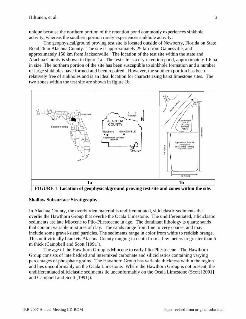
The geophysical/ground proving test site is located outside of Newberry, Florida on State Road 26 in Alachua County. The site is approximately 29 km from Gainesville, and approximately 150 km from Jacksonville. The location of the test site within the state and Alachua County is shown in figure 1a. The test site is a dry retention pond, approximately 1.6 ha in size. The northern portion of the site has been susceptible to sinkhole formation and a number of large sinkholes have formed and been repaired. However, the southern portion has been relatively free of sinkholes and is an ideal location for characterizing karst limestone sites. The two zones within the test site are shown in figure 1b.

1a 1b

FIGURE 1 Location of geophysical/ground proving test site and zones within the site. Shallow Subsurface Stratigraphy In Alachua County, the overburden material is undifferentiated, siliciclastic sediments that overlie the Hawthorn Group that overlie the Ocala Limestone. The undifferentiated, siliciclastic sediments are late Miocene to Plio-Pliestocene in age. The dominant lithology is quartz sands that contain variable mixtures of clay. The sands range from fine to very coarse, and may include some gravel-sized particles. The sediments range in color from white to reddish orange. This unit virtually blankets Alachua County ranging in depth from a few meters to greater than 6 m thick (Campbell and Scott [1991]).

The age of the Hawthorn Group is Miocene to early Plio-Pliestocene. The Hawthorn Group consists of interbedded and intermixed carbonate and siliciclastics containing varying percentages of phosphate grains. The Hawthorn Group has variable thickness within the region and lies unconformably on the Ocala Limestone. Where the Hawthorn Group is not present, the undifferentiated siliciclastic sediments lie unconformably on the Ocala Limestone (Scott [2001] and Campbell and Scott [1991]).


Hiltunen, et al. 4

Underlying the Hawthorn Group or the undifferentiated, siliciclastic sediments is the Ocala Limestone, which is Upper Eocene in age. It consists of nearly pure limestone and dolostones (Scott [2001]). The top of the limestone is extremely variable due to karstification and erosion. Features in Karstic Limestone Karst is a type of topography formed in unconsolidated sediments (soils) that overlie limestone, dolomite, or other soluble rock. The surface of the soluble rock may be erratic and highly variable indicating that chemical dissolution/weathering is presently occurring or had occurred before the soil was deposited, or the surface may be relatively flat indicating that chemical dissolution/weathering has not extensively occurred. The term “karstic limestone” is used to describe a limestone lithology that has undergone chemical weathering.

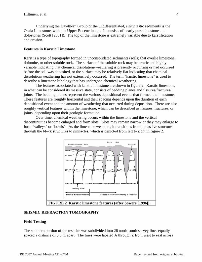
The features associated with karstic limestone are shown in figure 2. Karstic limestone, in what can be considered its massive state, consists of bedding planes and fissures/fractures/ joints. The bedding planes represent the various depositional events that formed the limestone. These features are roughly horizontal and their spacing depends upon the duration of each depositional event and the amount of weathering that occurred during deposition. There are also roughly vertical features within the limestone, which can be described as fissures, fractures, or joints, depending upon their geologic formation.

Over time, chemical weathering occurs within the limestone and the vertical discontinuities become enlarged and form slots. Slots may remain narrow or they may enlarge to form “valleys” or “bowls”. As the limestone weathers, it transitions from a massive structure through the block structures to pinnacles, which is depicted from left to right in figure 2.

FIGURE 2 Karstic limestone features (after Sowers [1996]).

SEISMIC REFRACTION TOMOGRAPHY Field Testing The southern portion of the test site was subdivided into 26 north-south survey lines equally spaced a distance of 3.0 m apart. The lines were labeled A through Z from west to east across


Hiltunen, et al. 5

the site, and each line was 85.3 m long, with station 0 m located at the southern end of the site. Two 36.6-m long refraction tests were conducted during summer 2005 end-to-end along lettered site lines A, F, K, P, U, and Z, and beginning at station 0. Thus, the 12 refraction tests covered six of the site lines from station 0 to 73.2 m.

Each 36.6-m long refraction test was conducted with 4.5 Hz vertical geophones spaced equally at 0.61 m, for a total of 61 measurements. Seismic energy was created by vertically striking a metal ground plate with an 89 N sledgehammer, thus producing compression wave (P-wave) first arrivals. Shot locations were spaced at 3.0-m intervals along the 36.6-m line and starting at 0 m, for a total of 13 shots. Since a 32-channel dynamic signal analyzer was used to collect time records, and each line required 61 measurements, each line was conducted in two stages. In stage one, 31 geophones were placed at 0.61-m intervals from station 0 m to station 18.3 m. In stage two, 31 geophones were placed at 0.61-m intervals from station 18.3 m to station 36.6 m. Since there was a designed overlap between the two stages at station 18.3 m, a total of 61 measurement locations were collected. For each stage, time records were collected at each of the 13 shot locations, and then the data were combined to produce a complete shot gather for the survey line from station 0 m to station 36.6 m.

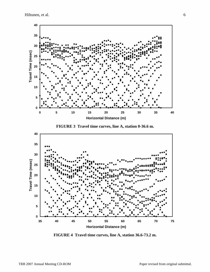
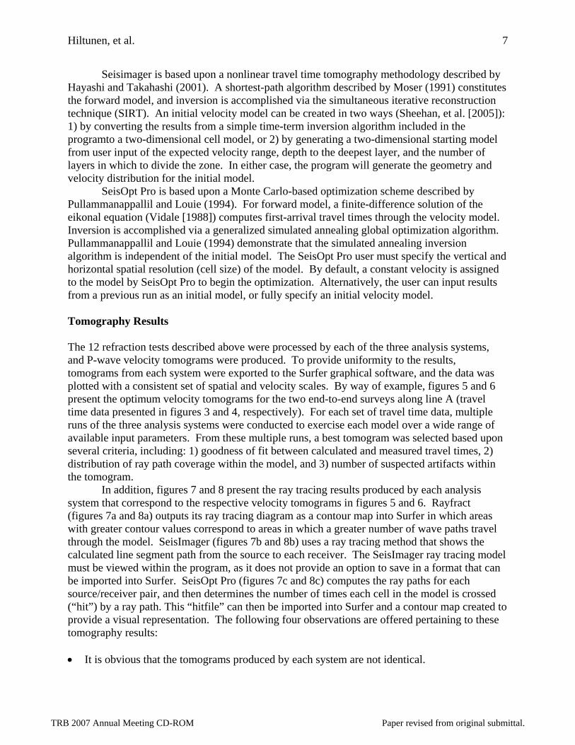
Travel time records were transferred to the PickWin program (a module of the Seisimager refraction system described below), where geophone and shot geometry were implanted with the records, and first arrivals were determined and saved for analysis with three tomography programs. By way of example, first-arrival travel time curves for the two end-to-end surveys along the line A are shown in figures 3 and 4. Data for line A was chosen for presentation herein because these refraction results displayed the most variable conditions along the line, and this line consequently received considerable attention during intrusive ground proofing investigations described below. Tomography Programs Three commercially-available refraction tomography software systems were used to produce P-wave velocity tomograms for each of the 12 travel time data sets. The three systems, Rayfract, Seisimager, and SeisOpt Pro, are well described by their authors, and in several recent publications by users of these systems. The following statements provide a very brief overview, as well as a listing of key references for the reader to locate further details. Each of the systems contains three important components: 1) a forward model for calculating source to receiver first arrival times based upon the current velocity model, 2) an inversion routine for adjusting the velocity model until an acceptable match between calculated and measured first-arrival travel times is obtained, and 3) a means for generating an initial velocity model.

Rayfract is based upon the wavepath eikonal travel time (WET) inversion method of Schuster and Quintus-Bosz (1993). The WET inversion method is founded upon a back-projection formula for inverting velocities from travel times computed by a finite-difference solution to the eikonal equation (Qin, et al. [1992]). Rayfract provides two options for generating an initial model to start WET inversion: 1) use the Delta-t-V method included in Rayfract, or 2) use the “smooth inversion” algorithm that automatically creates a one-dimensional model based on Delta-t-V results that is then extended to cover the two-dimensional area (Sheehan, et al. [2005]). The “smooth inversion” algorithm is intended to eliminate artifacts that can sometimes be produced by the Delta-t-V solutions.


Hiltunen, et al. 6

FIGURE 3 Travel time curves, line A, station 0-36.6 m.

FIGURE 4 Travel time curves, line A, station 36.6-73.2 m.

0

5

10

15

20

25

30

35

40

0 5 10 15 20 25 30 35 40

Horizontal Distance (m)

Trav

el T

ime

(mse

c)

0

5

10

15

20

25

30

35

40

35 40 45 50 55 60 65 70 75

Horizontal Distance (m)

Trav

el T

ime

(mse

c)


Hiltunen, et al. 7

Seisimager is based upon a nonlinear travel time tomography methodology described by Hayashi and Takahashi (2001). A shortest-path algorithm described by Moser (1991) constitutes the forward model, and inversion is accomplished via the simultaneous iterative reconstruction technique (SIRT). An initial velocity model can be created in two ways (Sheehan, et al. [2005]): 1) by converting the results from a simple time-term inversion algorithm included in the programto a two-dimensional cell model, or 2) by generating a two-dimensional starting model from user input of the expected velocity range, depth to the deepest layer, and the number of layers in which to divide the zone. In either case, the program will generate the geometry and velocity distribution for the initial model.

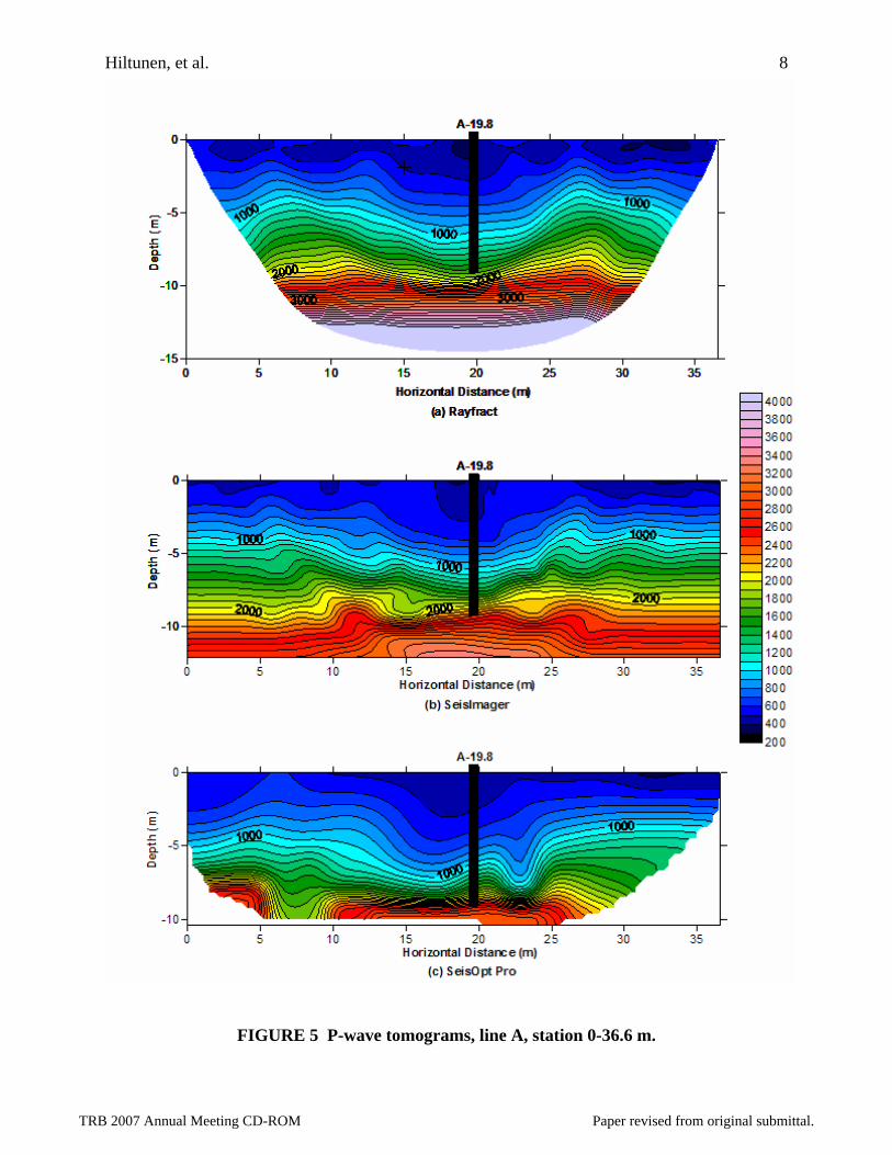
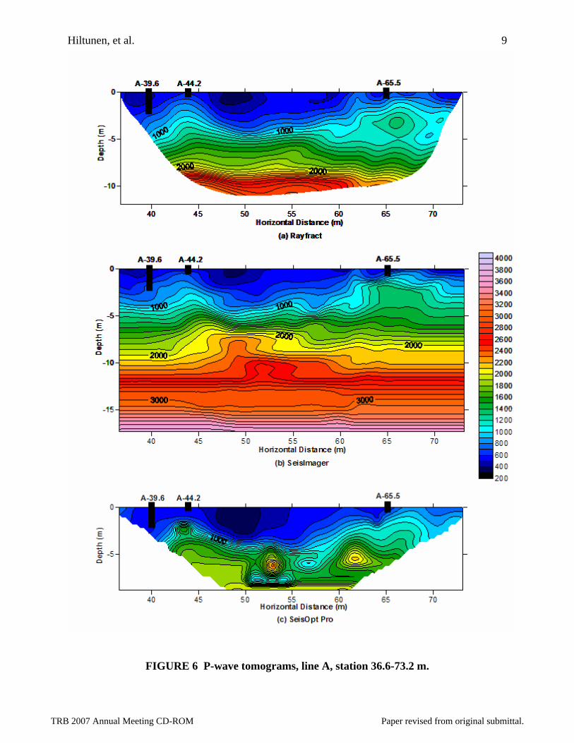
SeisOpt Pro is based upon a Monte Carlo-based optimization scheme described by Pullammanappallil and Louie (1994). For forward model, a finite-difference solution of the eikonal equation (Vidale [1988]) computes first-arrival travel times through the velocity model. Inversion is accomplished via a generalized simulated annealing global optimization algorithm. Pullammanappallil and Louie (1994) demonstrate that the simulated annealing inversion algorithm is independent of the initial model. The SeisOpt Pro user must specify the vertical and horizontal spatial resolution (cell size) of the model. By default, a constant velocity is assigned to the model by SeisOpt Pro to begin the optimization. Alternatively, the user can input results from a previous run as an initial model, or fully specify an initial velocity model. Tomography Results The 12 refraction tests described above were processed by each of the three analysis systems, and P-wave velocity tomograms were produced. To provide uniformity to the results, tomograms from each system were exported to the Surfer graphical software, and the data was plotted with a consistent set of spatial and velocity scales. By way of example, figures 5 and 6 present the optimum velocity tomograms for the two end-to-end surveys along line A (travel time data presented in figures 3 and 4, respectively). For each set of travel time data, multiple runs of the three analysis systems were conducted to exercise each model over a wide range of available input parameters. From these multiple runs, a best tomogram was selected based upon several criteria, including: 1) goodness of fit between calculated and measured travel times, 2) distribution of ray path coverage within the model, and 3) number of suspected artifacts within the tomogram.

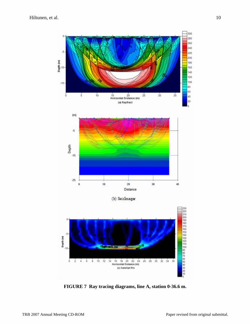
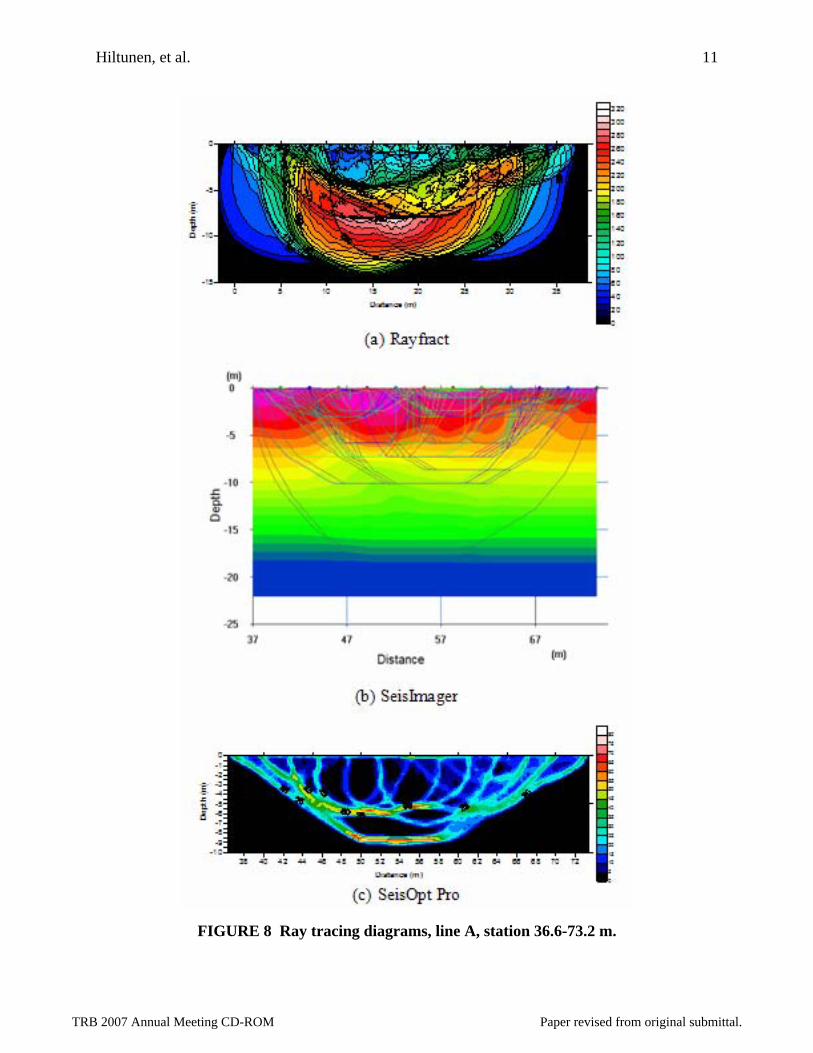
In addition, figures 7 and 8 present the ray tracing results produced by each analysis system that correspond to the respective velocity tomograms in figures 5 and 6. Rayfract (figures 7a and 8a) outputs its ray tracing diagram as a contour map into Surfer in which areas with greater contour values correspond to areas in which a greater number of wave paths travel through the model. SeisImager (figures 7b and 8b) uses a ray tracing method that shows the calculated line segment path from the source to each receiver. The SeisImager ray tracing model must be viewed within the program, as it does not provide an option to save in a format that can be imported into Surfer. SeisOpt Pro (figures 7c and 8c) computes the ray paths for each source/receiver pair, and then determines the number of times each cell in the model is crossed (“hit”) by a ray path. This “hitfile” can then be imported into Surfer and a contour map created to provide a visual representation. The following four observations are offered pertaining to these tomography results: • It is obvious that the tomograms produced by each system are not identical.


Hiltunen, et al. 8

FIGURE 5 P-wave tomograms, line A, station 0-36.6 m.


Hiltunen, et al. 9

FIGURE 6 P-wave tomograms, line A, station 36.6-73.2 m.


Hiltunen, et al. 10

FIGURE 7 Ray tracing diagrams, line A, station 0-36.6 m.


Hiltunen, et al. 11

FIGURE 8 Ray tracing diagrams, line A, station 36.6-73.2 m.


Hiltunen, et al. 12

• Seisimager produces a tomogram rectangular in shape, while tomograms from Rayfract and

SeisOpt Pro are bowl or pyramidal in shape. In fact, there is little or no ray path coverage near the model edges (figures 7 and 8), and Rayfract and SeisOpt Pro trim the edges to demonstrate that measured rays have not passed through these zones. On the other hand, Seisimager appears to extrapolate the interior of the model to produce a rectangular shape.

• The contouring of the Rayfract models is generally smoother, while the Seisimager and SeisOpt Pro models are more variable. The SeisOpt Pro models in particular even display some strange features within the lower half, and these features typically occur in regions of low ray path coverage as demonstrated by the results shown in figures 7c and 8c.

• The gross features of the site profile are consistently delineated by each of the three systems, particularly if one concentrates on the upper half of each model where the ray coverage is most dense. In this regard, the two line A results are similar: there appears to be a valley/ bowl near the middle, and blocks/pinnacles near the left and right ends. Results from each of the three systems suggest this profile interpretation.

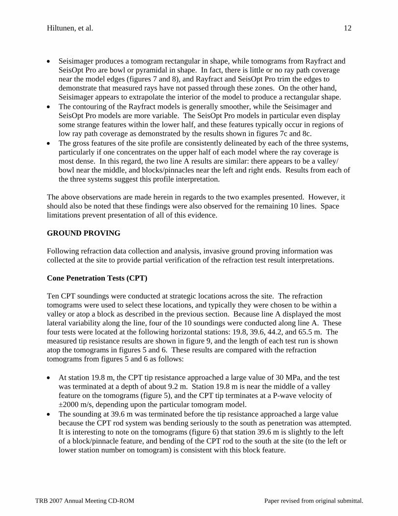
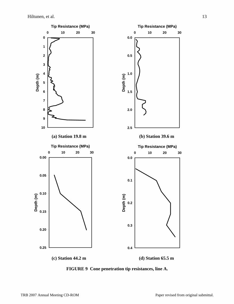
The above observations are made herein in regards to the two examples presented. However, it should also be noted that these findings were also observed for the remaining 10 lines. Space limitations prevent presentation of all of this evidence. GROUND PROVING Following refraction data collection and analysis, invasive ground proving information was collected at the site to provide partial verification of the refraction test result interpretations. Cone Penetration Tests (CPT) Ten CPT soundings were conducted at strategic locations across the site. The refraction tomograms were used to select these locations, and typically they were chosen to be within a valley or atop a block as described in the previous section. Because line A displayed the most lateral variability along the line, four of the 10 soundings were conducted along line A. These four tests were located at the following horizontal stations: 19.8, 39.6, 44.2, and 65.5 m. The measured tip resistance results are shown in figure 9, and the length of each test run is shown atop the tomograms in figures 5 and 6. These results are compared with the refraction tomograms from figures 5 and 6 as follows: • At station 19.8 m, the CPT tip resistance approached a large value of 30 MPa, and the test

was terminated at a depth of about 9.2 m. Station 19.8 m is near the middle of a valley feature on the tomograms (figure 5), and the CPT tip terminates at a P-wave velocity of ±2000 m/s, depending upon the particular tomogram model.

• The sounding at 39.6 m was terminated before the tip resistance approached a large value because the CPT rod system was bending seriously to the south as penetration was attempted. It is interesting to note on the tomograms (figure 6) that station 39.6 m is slightly to the left of a block/pinnacle feature, and bending of the CPT rod to the south at the site (to the left or lower station number on tomogram) is consistent with this block feature.


Hiltunen, et al. 13

(a) Station 19.8 m (b) Station 39.6 m

(c) Station 44.2 m (d) Station 65.5 m

FIGURE 9 Cone penetration tip resistances, line A.

0

1

2

3

4

5

6

7

8

9

10

0 10 20 30

Tip Resistance (MPa)

Dep

th (m

)0.0

0.5

1.0

1.5

2.0

2.5

0 10 20 30


Dep

th (m

)

0.00

0.05

0.10

0.15

0.20

0.25

0 10 20 30


Dep

th (m

)

0.0

0.1

0.2

0.3

0.4

0 10 20 30


Dep

th (m

)


Hiltunen, et al. 14

• At stations 44.2 and 65.5 m the tests were terminated at shallow depths less than 0.5 m because the CPT tip resistance approached a large value of 30 MPa. Stations 44.2 and 65.5 m are both located near the top of block/pinnacle features on the tomograms (figure 6). However, in contrast to station 19.8 m, the CPT tips terminated at P-wave velocities less than 1000 m/s at stations 44.2 and 65.5 m.

• It is reported that small, rock outcrops were visible near stations 62.5-64 m and 66.1-67.1 m, which are on both sides of the CPT sounding at 65.5 m.

• Finally, it is reported that similar results as described above were discovered for the remaining six CPT soundings across the site. Three “deep” soundings terminated within valleys/bowls on the tomograms. Three “shallow” soundings terminated near the top of block/pinnacle features on the tomograms at relatively lower P-wave velocities as compared to the “deep” soundings.

Geotechnical Borings and Standard Penetration Tests (SPT) Eight geotechnical borings and SPT soundings were conducted at strategic locations across the site. Similar to above, the refraction tomograms and CPT results were used to select these locations. All of the borings included drilling and recovery of rock cores through a minimum of 3 m of material, and in one core, through 11 m of material. While space limitations do not allow presentation of these detailed boring log results herein, the following information is provided: • Three of the eight borings were located along line A at the following stations: 19.8, 35.6, and

65.5 m. These borings coincided with CPT tests at 19.8 and 65.5, while the boring at 35.6 m was slightly to the left of the CPT sounding at 39.6 m.

• At station 19.8 m, the boring was advanced through predominantly sand overburden soil having SPT N-values less than 10 to a depth of 9.0 m. Below 9.0 m, coring was conducted to a depth of 12.5 m, and the material was reported to be tan limestone with fossils throughout. The recovery of this material was 100% throughout, and the rock quality designation (RQD) was reported as 100, except for the first 0.5 m which was broken at the top (RQD approximately 85).

• At station 35.6 m, the boring was advanced through sandy clay and sand overburden soil having SPT N-values between 7 and 10 to a depth of 2.3 m. Below 2.3 m, coring was conducted to a depth of 11.0 m, and the material was reported to be predominantly light tan to white limestone with fossils throughout.

• At station 65.5 m, the boring was advanced through sand overburden soil to a depth of only 0.3 m. Below 0.3 m, coring was conducted to a depth of 9.4 m, and the material was reported to be predominantly light tan to white limestone with fossils throughout. The recovery of this material varied between 80-100%, with approximately 60% of the run reported at the 100% recovery level. The boring notes report that several zones appeared to be weak and broken, and the RQDs varied widely between 30 and 100. Nearly half the run indicated an RQD between 60 and 80, a short distance (10%) at RQD of 100, and the remaining 40% reported a RQD between 30 and 60.

These results are compared with the refraction tomograms from figures 5 and 6, and the CPT results from figure 9 as follows:


Hiltunen, et al. 15

• The CPT and boring information at stations 19.8 and 65.5 m appear to be in good agreement. At 19.8, CPT testing was terminated upon approaching a limiting large value at a depth of 9.2 m, while boring information reported the overburden soil/rock interface at a depth of 9.0 m. Similarly, at 65.5, CPT testing was terminated at a depth less than 0.5 m, while the top of rock was reported at 0.3 m.

• The undulating, valley/bowl to block/pinnacle features noted along the P-wave velocity tomograms appear to be the result of lateral variation in the overburden soil/rock interface along the length of the refraction line. At 19.8, a valley/bowl feature appears, and the top of rock is found at 9.0 m, while at 65.5, a block/pinnacle feature appears, and the top of rock is found at 0.3 m.

• While the undulating features in the velocity tomograms are generally indicative of the soil/rock interface, the top of rock does not appear along a constant contour of P-wave velocity. Within a valley (station 19.8), the top of rock is found at approximately 2000 m/s, while at the top of a block (station 65.5), the top of rock is found at a velocity of approximately 500 m/s. However, the rock under station 19.8 m was reported competent and intact, with 100% recovery and RQD of 100 throughout all but a short length at top of core run, while the rock under station 65.5 m was reported to be of lower quality. Velocity differences between these two materials should be expected.

• Finally, it is interesting to note that the CPT appears to penetrate a particulate, sand material of higher velocity (station 19.8) easier than it will a rock of lower velocity (station 65.5). A possible explanation is as follows. Velocity is related to the small-strain modulus of the material, while CPT tip resistance is related to bearing capacity or strength of the material. Even though the rock at station 65.5 has a relatively low velocity as measured through a large volume of material, the local strength beneath the cone tip is still large. A large, broken mass of this material under low confinement near the ground surface has low velocity. However, the local, broken pieces are still an intact, cemented material, and highly resistant to local CPT penetration. Alternatively, the particulate, sand material under large confinement at 9 m is considerably stiffer, yet will undergo local shear failure under CPT penetration. Thus, these results reinforce the premise that good site characterization practice should include measurement of multiple parameters to fully understand expected behavior.

Geological Explanations for Variability in Velocity Measurements The limestone bedrock (Ocala Limestone) was formed in the Upper Eocene age (Scott [1991]). The limestone itself was formed in a variety of environments, notably open marine, shallow water, and middle shelf deposition, and there is a wide variety of organisms that contributed to the formation of the limestone. The upper surface of the Ocala Limestone has undergone extensive dissolution during a major sea-level drop that occurred during the late Oligocene and Miocene. This event is the precursor to the karst terrain that later developed (Randazzo [1997]).

As discussed above, there is a marked difference between the top of bedrock velocities measured at the bottom of limestone valleys and the top of blocks or pinnacles. The weathering/ dissolution/karstification occurred from the top down; the upper limestone surface was the first to be weathered. Limestone that was more susceptible to weathering was dissolved, forming the slots/valleys within the karst terrain. Weathering within these zones was diminished when the limestone became more competent at depth. What remained was the block and pinnacle structures, which are the most competent of the highest weathered rock. As expected, the


Hiltunen, et al. 16

measured compression wave velocities are highest within the limestone valleys and lowest at the tops of blocks and pinnacles. CONCLUSIONS Karstic limestone is characterized by a typically undulating bedrock surface and the presence of numerous springs, cavities, and caves. Analysis of a seismic refraction study at the shared University of North Florida and University of Florida karstic limestone geophysical/ground proving test site in central Florida demonstrated that three commercially-available refraction tomography software systems are able to reveal the typical undulating bedrock surface. In comparison, tomograms from Rayfract and SeisOpt Pro are bowl or pyramidal in shape because there is little or no ray path coverage near the model edges, while Seisimager appears to extrapolate the interior of the model beyond the area of ray coverage to produce a rectangular shape. This information near the model edges should be used with caution. Also, contouring of the Rayfract models is generally smoother, while the Seisimager and SeisOpt Pro models are more variable. In particular, models from SeisOpt Pro often display some strange features within the lower half. These features typically occur in regions of low ray path coverage, and these areas should be viewed with caution.

With respect to subsurface conditions at the test site, compression wave velocities at the top of bedrock within limestone valleys were significantly higher than compression wave velocities at the top of blocks and pinnacles. Ground proving via cone penetration tests and geotechnical borings indicates that the material is indeed limestone at both location types, and demonstrates the importance of measuring multiple material parameters during site characterization activities in complex terrane. The variability in bedrock condition is attributed to the geological history of the limestone, which includes how the limestone was formed and how the limestone is weathered. ACKNOWLEDGEMENTS This work was supported by the Florida Department of Transportation, District 2, under UNF project number 230117000. REFERENCES Campbell, K. M. and Scott, T. M. (1991), “Radon Potential Study, Alachua County, Florida: Near-Surface Stratigraphy and Results of Drilling,” Florida Geological Survey Open File Report Number 41, 15 pp. Carpenter, P. J., Higuera-Diaz, I. C., Thompson, M. D., Atre, S., and Mandell, W. (2003), “Accuracy of Seismic Refraction Tomography Codes at Karst Sites,” Geophysical Site Characterization: Seeing Beneath the Surface, Proceedings of a Symposium on the Application of Geophysics to Engineering and Environmental Problems, San Antonio, Texas, April 6-10, pp. 832-840.


Hiltunen, et al. 17

Cramer, B. J. and Hiltunen, D. R. (2004), “Investigation of Bridge Foundation Sites in Karst Terrane via Seismic Refraction Tomography,” 83rd Annual Meeting Compendium of Papers CD-ROM, Transportation Research Board, Washington, D.C., January 11-15. Hayashi, K. and Takahashi, T. (2001), “High Resolution Seismic Refraction Method Using Surface and Borehole Data for Site Characterization of Rocks,” International Journal of Rock Mechanics and Mining Sciences, Vol. 38, pp. 807-813. Hiltunen, D. R. and Cramer, B. J. (2006), “Geophysical Characterization of Bridge Foundation Sites in Karst Terrane,” 85th Annual Meeting Compendium of Papers CD-ROM, Transportation Research Board, Washington, D.C., January 22-26. Moser, T. J. (1991), “Shortest Path Calculation of Seismic Rays,” Geophysics, Vol. 56, No. 1, January, pp. 59-67. Pullammanappallil, S. K. and Louie, J. N. (1994), “A Generalized Simulated-Annealing Optimization for Inversion of First-Arrival Times,” Bulletin of the Seismological Society of America, Vol. 84, No. 5, October, pp. 1397-1409. Qin, F., Luo, Y., Olsen, K., Cai, W., and Schuster, G. T. (1992), “Finite-Difference Solution of the Eikonal Equation,” Geophysics, Vol. 57, pp. 478-487. Randazzo, A. F. (1997), “The Sedimentary Platform of Florida: Mesozoic to Cenozoic,” The Geology of Florida, Randazzo, A. F. and Jones, D. S., Ed., University of Florida Press, Gainesville, FL. Schuster, G. T. and Quintus-Bosz, A. (1993), “Wavepath Eikonal Traveltime Inversion: Theory,” Geophysics, Vol. 58, No. 9, September, pp. 1314-1323. Scott, T. M. (2001), “Text to Accompany the Geologic Map of Florida,” Florida Geological Survey Open File Report Number 80, 28 pp. Sheehan, J., Doll, W., and Mandell, W. (2005), “An Evaluation of Methods and Available Software for Seismic Refraction Tomography Analysis,” Journal of Environmental and Engineering Geophysics, Vol. 10, No. 1, March, pp. 21-34. Sowers, G. (1996), Building on Sinkholes – Design and Construction of Foundations in Karst Terrain, ASCE Press, New York. Vidale, J. E. (1988), “Finite Difference Calculation of Travel Times,” Bulletin of the Seismological Society of America, Vol. 78, pp. 2062-2076.


Documents

GROUND PROVING THREE SEISMIC REFRACTION TOMOGRAPHY …