Grid Fundamentals

Ian A. HiskensVennema Professor of Engineering

Professor, Electrical Engineering and Computer Science

Grid Science Winter SchoolSanta Fe, NM

January 12, 2015

Power system overview

2/66

Structure1. Power Flow2. Generator modelling3. Generator control4. Load modelling5. Substations6. Protection

3/66

Power flow formulation• The power flow determines the (complex) voltage at every node

in a network, given:– Generator power injections and voltage set-points.– Load active and reactive power demands.– Network impedances.

• Linear network model given by Kirchhoff’s laws.• Nonlinear boundary conditions at nodes due to constant power

injections.

PQ node

PQ node PV node

Slack node• Angle reference.• Balance active

power.

4/66

Power flow equations

5/66

Jacobian• Power flow sensitivities are given by the Jacobian:

For

6/66

Voltage – reactive power coupling• Under “normal” power system conditions,

and .• It follows that and are small, and power flow

interactions are dominated by the and couplings.– When the network is heavily loaded, may not be small.– For distribution and subtransmission networks, ratios

are higher, so ignoring may not provide a good approximation.

7/66

Radial networks• For radial networks, the power flow equations can be written in the

recursive form:

where is the set of nodes connected “downstream” of node , and the branch impedance is .

• This set of equations can be solved using a simple forward/backward iterative algorithm.

8/66

Resistance in the network• The relationship between injected

power and the bus voltage magnitude is given by,

9/66

Power flow solution• The power flow problem (neglecting limits) can be expressed as:

where consists of voltage magnitudes and angles, are parameters such as:– Active and reactive power at PQ buses.– Active power and voltage magnitude at PV buses.– Distance in a particular loading direction:

• For a system of buses, has dimension (if the mismatch at the slack is included as a state), and has dimension .

• With all parameters specified (fixed), consists of equations in variables.– Solutions are isolated points, but there are generally multiple solutions.

10/66

Multiple solutions

11/66

Newton solution• Solutions can be obtained using a Newton iterative process:

where indicates the iteration number, and is the Jacobian matrix

which has dimension , and is very sparse.

• Iterative techniques such as Newton's method are generally not globally convergent.

• They require an initial guess that lies in the “region of convergence”.

12/66

Maximum loadability• Notice from the “bifurcation diagram”

that as increases, the solutions and move closer together, eventually coalescing at .

• As and move closer together, their associated regions of convergence shrink.

• It is more difficult to find an initial guess that gives convergence.

• No solutions exist for .• The critical point at , the maximum value of for which a solution

exists, is called a saddle node bifurcation.• The Jacobian is singular at that point.• Voltages (given by ) become infinitely sensitive to load changes (given

by .)

13/66

Point of collapse• If the load increases beyond , no steady-state

(equilibrium) solutions exist, so transient response has nowhere to settle.

• Typically voltages across a region of the power system decline uncontrollably to low values, initiating protection operation.

• The maximum loadability point is also called the point of collapse.

• The point of collapse describes the absolute limiting case for system loading.

• Many security margins are defined in terms of a norm (distance) from the operating point to that limiting case.

14/66

Power flow divergence• The power flow solution process becomes unreliable

near maximum loadability.• Newton solution relies on , but approaches

singularity (becomes ill-conditioned.)• It is important to note that maximum loadability

implies power flow non-convergence, but power flow non-convergence does not necessarily imply maximum loadability.– Many power flow programs may exhibit poor convergence a

long way from maximum loadability.

15/66

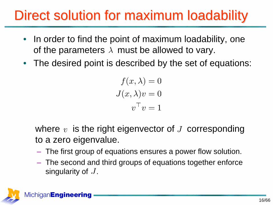
Direct solution for maximum loadability• In order to find the point of maximum loadability, one

of the parameters must be allowed to vary.• The desired point is described by the set of equations:

where is the right eigenvector of corresponding to a zero eigenvalue.– The first group of equations ensures a power flow solution.– The second and third groups of equations together enforce

singularity of .

16/66

Direct solution• Number of equations is .• Number of variables:

contributes .contributes .contributes 1.

• Number of equations and variables are equal, giving point solutions.

• Obtaining a solution may be difficult though, as choosing appropriate initial values for , , and (required by the iterative solution process) can be challenging.

• Direct solution gives the point of maximum loadability, but tells nothing about the variation in system conditions as the load increases towards the maximum.

• This extra information can be obtained using a continuation process.

17/66

Continuation power flow• Consider the power flow problem

where is a single free parameter.• This problem has variables but only equations, so is

under-determined.– The solution is a curve.

18/66

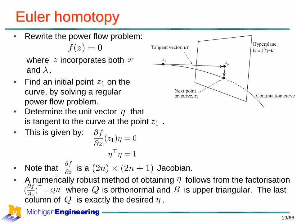
Euler homotopy• Rewrite the power flow problem:

where incorporates both and .

• Find an initial point on the curve, by solving a regular power flow problem.

• This is given by:

• Note that is a Jacobian.• A numerically robust method of obtaining follows from the factorisation

where is orthonormal and is upper triangular. The last column of is exactly the desired .

• Determine the unit vector that is tangent to the curve at the point .

19/66

Euler homotopy (2)• The prediction of the next point on the curve is given by:

where is the size of the step taken in the direction of the tangent vector .

• The correction to a point on the curve is then made. This is achieved by solving for the point of intersection of:– The solution curve, and– A hyperplane that passes through and that is orthogonal

to . Points on this hyperplane are given by

which is equivalent to .• The desired point is given by solving:

20/66

Euler homotopy (3)

• Once two points have been calculated, the tangent vector can be formed by the secant approximation:

• The approximation may not be adequate when the curve has high curvature.

21/66

Structure1. Power Flow2. Generator modelling3. Generator control4. Load modelling5. Substations6. Protection

22/66

Basic synchronous machine equations

From Sauer and Pai

23/66

Park’s transformation• The sinusoidal steady-state of balanced symmetrical

machines can be transformed to produce constant states. Define:

where

24/66

Further steps• Energy balance gives:

• Define an angle that is constant for constant shaft speed:

• Scale using per unit – many degrees of freedom.• Establish the relationship between flux linkages and

currents:

25/66

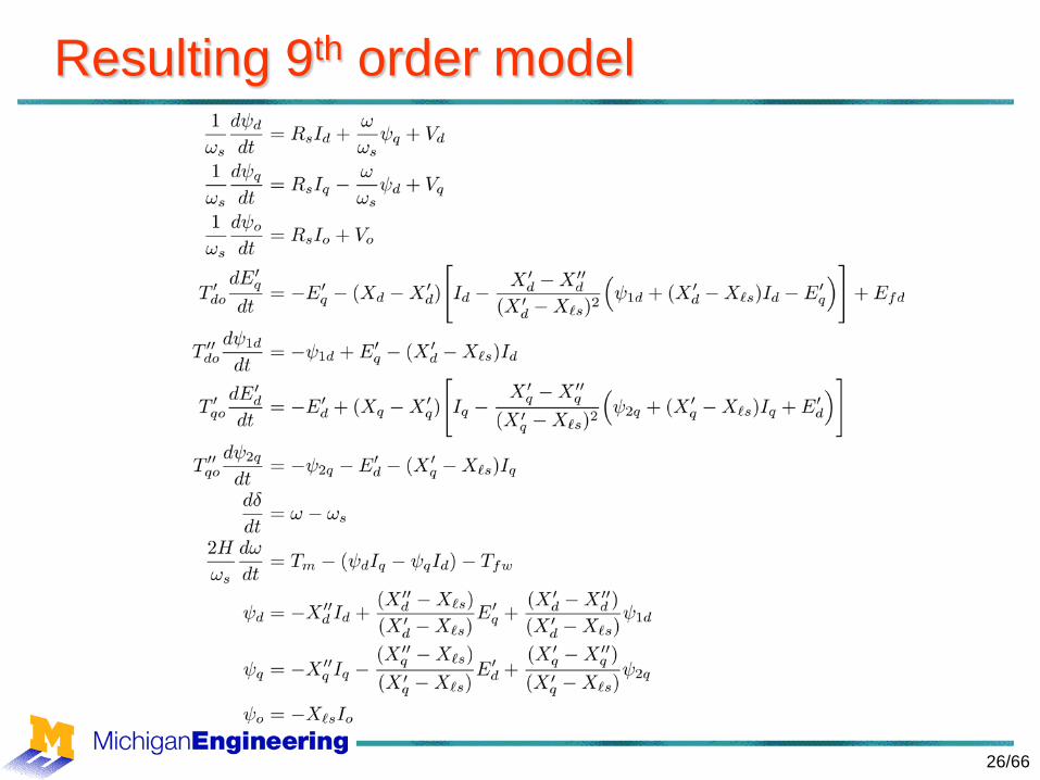
Resulting 9th order model

26/66

Terminal conditions• Consider a balanced set of sinusoidal voltages and currents:

• Park’s transformation together with appropriate per unit scaling give:

27/66

Elimination of stator transients• The time constants associated with and are small

relative to the other machine dynamics.• Under balanced conditions, is zero.• The resulting 6th order model becomes:

The original differential equations are replaced by algebraic equations:

28/66

Two-axis model• If and are sufficiently small, the damper winding states

and can be eliminated by setting , giving:

29/66

One-axis model• If is sufficiently small, the remaining damper winding state

can be eliminated by setting , giving:

30/66

Classical model• Assume is large, so that is effectively constant.• Assume and .• The resulting model has no electrical dynamics, only mechanical

dynamics:

with

or equivalently, multiplying throughout by ,

– Voltage source (with constant magnitude) behind transient reactance .

31/66

Structure1. Power Flow2. Generator modelling3. Generator control4. Load modelling5. Substations6. Protection

32/66

Generator voltage control• Voltage control is achieved by the automatic voltage regulator (AVR).

– Terminal voltage is measured and compared with a set-point.– The voltage error is driven to zero by adjusting the field voltage .

• An increase in the field voltage will result in an increase in the terminal voltage and in the reactive power produced by the generator.

• If field voltage becomes excessive, an over-excitation limiter will operate to reduce the field current.– The terminal voltage will subsequently fall.

33/66

High gain instability• As the AVR gain is increased, a Hopf bifurcation may lead to

oscillatory instability.

AVR gain

34/66

Power system stabilizers• High-gain voltage control can destabilize angle

dynamics.• To compensate, many generators have a power

system stabilizer (PSS) to improve damping.

35/66

Governor• Active power regulation is achieved by a governor.

– If frequency is less than desired, increase mechanical torque.– Decrease mechanical torque if frequency is high.

• For a steam plant, torque is controlled by adjusting the steam value, for a hydro unit control vanes regulate the flow of water delivered by the penstock.

• Frequency is a common signal seen by all generators.– If all generators tried to

regulate frequency to its nominal setpoint, hunting would result.

– This is overcome through the use of a droop characteristic.

36/66

Automatic generation control (AGC)• Based on a control area

concept (now called a balancing authority.)

• Each balancing authority generates an “area control error” (ACE) signal,

where is the frequency bias factor.

• The ACE signal is used by AGC to adjust governor setpoints at participating generators.• This restores frequency and tie-line flows to their scheduled values.• Economic dispatch operates on a slower timescale to re-establish the

most economic generation schedule.

37/66

Structure1. Power Flow2. Generator modelling3. Generator control4. Load modelling5. Substations6. Protection

38/66

Load modelling• Work is always on-going…• Three philosophies:

1. Very simple generic load models. Static models have the form,

The so-called ZIP model is composed of three terms: constant impedance, constant current and constant power.

2. Use disturbance measurements to estimate parameters of generic load models that (supposedly) capture aggregate load behaviour.

3. Undertake a detailed assessment of the load composition (amounts of various load categories) at load locations (distribution substations) that exert an important influence on system behaviour.

• Distributed generation further complicates load modelling.39/66

Generic load recovery• Load response to a voltage step typically consists of

an initial step followed by a recovery phase.

40/66

Load recovery model• A commonly used generic dynamic load model has the form,

where is the active power drawn from the system,describes the transient response of the load, and gives the steady-state load response, with

• The transient and steady-state changes, and the rate of recovery, are load dependent.– For induction motors, the recovery is very fast.– For aggregated distribution loads that are dominated by tap-

changing transformers, recovery is slow.

41/66

Load recovery model behaviour• When a disturbance (step change) in voltage occurs, the load

state cannot change instantaneously. Load demand will vary instantaneously in response to the change in voltage according to .

• The load state will evolve over time, driven by the mismatch, and with a rate of change dictated by the time

constant . This process will continue until steady-state is reached, when .

• Reactive power load is handled in different ways.– Constant power factor.– Reactive power has the same form of response, but and

differ from their active power counterparts.– It is usual to assume the rate of recovery matches active power,

.• Numerous other forms of generic load models have been

proposed.

42/66

Induction motor loads• Induction motor slip is driven by:

43/66

Detailed load modelling• Member utilities of the Western Electricity Coordinating Council

(WECC) face difficulties with delayed voltage recovery.

44/66

WECC load model• The WECC load model task force has proposed the

following elaborate model.

45/66

WECC load model components• Distribution system impedance.

– As motor loads start to draw high current, the voltage seen by the loads will be lower than the supply point voltage.

• Distribution capacitors.– The reactive support drops with the square of the voltage seen

down the distribution feeder. This response is different from most loads, so the capacitors should be included separately.

• Distributed generation can also be included on bus~3 of this model.

• Air conditioning motor load.– In summer, this can be a significant component of the total load.– Most residential air conditioners are single phase induction motors,

which behave quite differently to three phase motors.– These motors stall in 3-5 cycles, and then draw significant current,

eventually tripping on thermal protection.

46/66

Residential AC tests• The following plots were obtained by ramping voltage

down to zero, and then ramping back up.

From WECC Load Modeling Task Force.

47/66

Load composition• For a place like Wisconsin, the load contributions

during a typical summer peak are given in the following table.

48/66

Load model comparison (1)• The ZIP (constant impedance plus constant current plus

constant power) voltage-dependent load model and the detailed model behave quite differently.

From Diaz de Leon and Kehrli, 2006.

49/66

Load model comparison (2)• Different motor models may exhibit quite different responses.

– For example, the two motor models CLOD and CIM5 that are available within PSS/E behave very differently.

From Diaz de Leon and Kehrli, 2006.

50/66

Structure1. Power Flow2. Generator modelling3. Generator control4. Load modelling5. Substations6. Protection

51/66

Typical substation layout

Equipment:2 – Overhead earth wire4 – Voltage transformer5 – Disconnect switch6 – Circuit breaker7 – Current transformer8 – Lightning arrester9 – Power transformer

52/66

Sensing equipment

Hair-pin/tank CT Top-core CT

Current transformersCapacitor voltage transformers (CVT)

CVT equivalent circuit

From ABB Instrument transformer application guide.

53/66

Structure1. Power Flow2. Generator modelling3. Generator control4. Load modelling5. Substations6. Protection

54/66

Faults on power systems• Most unplanned transmission outages result from people in

substations.• Lightning strikes are the cause of

most transmission system faults.• Lack of vegetation management

also contributes to line outages.– Example: August 2003

blackout of north-east America.

55/20

• Other causes of transmission system faults are many and varied:– Animals climbing towers.– Insulators used for target practice.– Ice storms.– Dust accumulation on insulators, leading to flashovers.– Etc.

• Most faults are single-line-to-ground.– Generally least severe.

• Solid three-phase-to-ground faults are the most severe, but quite uncommon.

Faults on power systems (cont)

56/20

Fault current paths

Current flow for a single lineto ground fault.

Impact of a Y-∆ transformer onfault current flow.

57/20

1. Protective systems must be selective.– Remove the fault as quickly as possible.– Remove no more of the system than is absolutely necessary.

2. Faults can occur in the protection equipment and circuit breakers, so all protection must be backed up.

3. Absolutely every piece of a power system must be covered by protection.– If it can’t be protected, then it can’t be built.

Protective relaying principles

58/20

• Simplest system to protect.• Common to use overcurrent protection.

– Current flow due to a fault is usually much higher than load current.

• Under fault conditions, the circuit breaker to the left of the fault should operate.

• If a relay/breaker fails to operate, the next breaker up-stream should operate as backup.– Backup protection must be slower

than primary protection, otherwise they would race to operate.

– This is called the coordination time.

Radial systems

59/20

• Consider various fault scenarios:– For a fault at point x, breakers B23 and B32 should operate.– Assuming radial-system relay coordination, B23 would operate faster than B21.– But for a fault at point y, B21 should operate faster than B23.– Simple overcurrent relays cannot be coordinated for this case.

• Relays must be directional.– They only respond to faults in their “forward” direction.– In the example, B21 would not see the fault at x, and B23 would not see the fault

at y.– Backup protection is still provided:

B12 backs up B23, and B32 backs up B21.• Directionality is achieved by considering the phase angle between bus

voltage and fault current.

• This situation arises when distributed generation is added to a radial system.

• Protection must be more sophisticated.

Systems with multiple sources

60/20

• Fault detection is achieved by summing all the currents into a component, and checking that Kirchhoff’s current law holds.– If the currents do not add to zero, the mismatch must be due to

a fault creating an extraneous path.• Uses:

– Generators.– Transformers.

Must take account of turns ratio, and winding configuration.

– Buses.– Lines and cables.

Differential protection

61/20

• Power systems are divided into primary protection zones.– Defined by the locations of current transformers (CTs).– A fault anywhere in the zone will cause all circuit breakers that bound

the zone to open, isolating the fault.• The arrangement of circuit breakers and CTs ensures that primary

protection zones overlap.– Every point in the system lies in at least one primary zone.– Circuit breakers are also protected.

Overlapping protection zones

62/20

• During a fault, the voltage drops and the current rises.

• Distance protection monitors the “apparent impedance”

seen looking along a feeder.– The “distance” to the fault is given (approximately) by .

• Example: If a fault causes the voltage to halve and the current to double.– Overcurrent protection sees a 2:1 change in current.– Distance protection sees a 4:1 change in apparent impedance.

Distance protection

63/20

• Distance protection operation depends on lying within one of the zone characteristics:– Zone 1: Reaches 80% of the line

length, , instantaneous trip.– Zone 2: Reaches 120% of the line

length, , delayed trip.– Zone 3: Reaches 160-200% of the

line length, delayed trip.• Zone 2 and 3 provide backup, in case

of primary protection failure.• The lengthy reach of zone 3

was a major contributing factor in the August 2003 blackout, and has now been disabled by many utilities.

Distance protection (cont)

64/20

Over/under-voltage protection• High voltages may cause insulation breakdown,

component damage.• Low voltages are responsible for:

– Induction motor stalling.– Contactors dropping out.– Power electronics misfiring.

• Protection operating characteristics often take account of the magnitude and duration of a disturbance.

• Undervoltage load shedding is also used to mitigate system-wide voltage collapse.

65/66

Questions?

66/66