Embed Size (px)
Citation preview

1
An Empirical Examination of the Pollution Haven Hypothesis for India: Towards a
Green Leontief Paradox?
Erik Dietzenbacher and Kakali Mukhopadhyay
Abstract:
This paper empirically examines the pollution haven hypothesis for India in the 1990s.
We calculate the extra CO2, SO2 and NOx emissions induced by one billion rupees of
additional exports. This is compared with the reduction of pollution caused by an increase
in the imports of the same size. In contrast to what the pollution haven hypothesis states
for developing countries, we find that India gains considerably from extra trade. Over
time, the gains have only increased, indicating that India has moved further away from
being a pollution haven. The outcome is robust to changes in the underlying assumptions.
Keywords: International trade, Environment, Pollution haven, Input-output analysis
JEL Classification Codes: F18, Q32, D57
Addresses:
Erik Dietzenbacher, Faculty of Economics, University of Groningen, PO Box 800,
9700 AV Groningen, The Netherlands.
e-mail: [email protected].
Kakali Mukhopadhyay, Centre for Development and Environment Policy, Indian Institute
of Management Calcuta, Joka, D.H. Road, Calcutta 700104, India.
e-mail: [email protected].

2
1. Introduction
International trade allows a country to partially disconnect its domestic economic and
ecological systems, because some of the consumed goods are produced in other countries
(Daly, 1993; Pearce and Warford, 1993; Proops et al., 1999). The environmental impacts
of producing such goods affect the ecological system of the exporting country (where
production takes place) rather than the ecological system of the importing country (where
consumption occurs). In this sense trade allows countries to move away from producing
environmentally sensitive (in terms of natural resources and pollution) activities.
The dominant trend in the world economy in the 1990s was towards liberalization
of trade. The debate on the effects of trade on the environment has gained much
importance because of the Kyoto and Montreal Protocols and the discussions on the role
of greenhouse gas emissions for global warming and climate change (see, for example,
UNFCCC, 1992; and Wyckoff and Roop, 1994). One of the environmental impacts
typically discussed in connection with trade liberalization are the composition effects.1
These occur when increased trade leads countries to specialize in industries where they
enjoy a comparative advantage. If this advantage stems from differences in production
technologies, it may well be that both partners benefit from trade. Although industries in
developing countries are generally characterized by pollution intensities (i.e. per unit of
gross output) that are higher than in developed countries, mutual benefits – in a Ricardian
context – would be expected. However, if the comparative advantage stems from
differences in environmental stringency, the composition effects of trade will exacerbate
existing environmental problems in the countries with relatively lax regulations. This is
known as the pollution haven effect.
This effect is typically felt to apply to developing countries. Several causes
contribute to this. First, the higher incomes in the developed countries generate a greater
demand for clean air and water. Similarly, in developing countries, with lower levels of
income and higher discount rates, extra earnings and jobs are valued higher, relative to
health and less pollution. Second, the relative costs of monitoring and enforcing pollution
standards are higher in developing countries, given the scarcity of trained personnel, the
difficulty of acquiring sophisticated equipment and the high marginal costs of
1 Other commonly discussed impacts are the scale effects (were trade causes an expansion of economicactivity and thus pollution) and the technological effects (were trade induces technology spillovers that leadto the adoption of “cleaner” production techniques). See, for example, OECD (1997), Jones (1998), andNordström and Vaughan (1999).

3
undertaking such a new governmental activity (when the policy focus is usually on
reducing fiscal burdens). Third, growth in developing countries results in a shift from
agriculture to manufacturing with rapid urban growth and substantive investments in
urban infrastructure, all of which raise the pollution intensity. In developed countries,
however, growth is associated with a shift from manufacturing to services, leading to a
decrease of the pollution intensity.
It is commonly assumed by economists and environmentalists that more economic
openness will lead to an increase of pollution in developing countries. Free trade will
induce displacement of “dirty” industries from developed countries with stricter
environmental regulations, and will raise the competitive pressure on developing
countries to reduce further their environmental standards.
Although the pollution haven hypothesis has received ample attention in the
literature, tests still seem to be largely lacking.2 In this paper we analyze the pollution
haven effect for India and its development over time. We calculate the pollution content
of one billion rupees of Indian exports and compare it with the pollution content that
would have been involved in producing one billion rupees of Indian imports at home (i.e.
in India). So, leaving the current account balance of India as it is, we answer the question
whether extra trade is beneficial in terms of pollution. For a pollution haven, we would
expect a negative answer.
The plan of the paper is as follows. In Section 2, we present the underlying model,
which is based on input-output techniques. The pollution haven hypothesis in the context
of the model is discussed in Section 3. The empirical tests for India are carried out in
Section 4, for the emissions of carbon, sulphur and nitrogen dioxides. The conclusions
are given in Section 5.
2. Methodology
Our starting point is the open, static input-output model (see e.g. Miller and Blair, 1985,
for an introduction), which is expressed as3
2 For a rare exception, see Eskeland and Harrison (2003) who have examined - using data on US foreigndirect investments - whether multinationals tend to flock to pollution havens in developing countries.3 Input-output techniques have been widely applied to determine the role of international trade inenvironmental damage. See, for example, Fieleke (1974); Wright (1974); Antweiler (1996); Proops et al.
4
z = Az + y (1)
where z is the 1×k vector of gross output in each of the k commodities, A is the kk ×
matrix of input coefficients, and y is the 1×k vector of final demands (including private
and government consumption and investments, gross exports and inventory changes).
The input coefficients ija are obtained as jijij zda /= , where ijd denotes the domestic
intermediate deliveries in million rupees (mrs) of commodity i to industry j. So, the input
coefficient ija thus indicates the input in mrs of commodity i per mrs of output of
commodity j.
Assuming fixed input coefficients, for any exogenously specified final demand
vector y~ , the solution of the input-output model in (1) is given by yLyAIz ~~)(~ 1 =−= − ,
where 1)( −−= AIL denotes the Leontief inverse. Its typical element ijl denotes the
output of commodity i (in mrs), required per mrs of final demand for commodity j. The
vector z~ gives the domestic gross outputs that need to be produced to satisfy the final
demands y~ .
The next step is to calculate how much input of fossil fuels is required to produce
z~ , and therefore is required (directly and indirectly) to satisfy final demands y~ . The
fossil fuels are given by commodities 1 (coal and lignite) and 2 (crude petroleum and
natural gas) – which shall be termed coal and oil for short. It is assumed that all the coal
and oil are combusted whenever they are used as an intermediate input, generating CO2,
SO2 and NOx emissions. It should be noted that it is not necessary that if, for example, the
industry that produces fertilizers uses inputs of crude oil, the actual combustion of crude
oil takes place in that industry. The assumption is that somewhere in the entire production
process that leads to a certain final demand (e.g. for fertilizers), all directly and indirectly
required coal and oil is combusted.
(1999); Lenzen (2001); Machado et al. (2001); Munksgaard and Pedersen (2001); and Kraines and Yoshida(2004).

5
Let us indicate the first two rows (corresponding to coal and oil) of the input
coefficients matrix A by 1a′ and 2a′ , respectively.4 The jth element of the row vector 1a′
then expresses the amount (in mrs) of domestically produced coal used as input for one
mrs of output of commodity j. To find the input of coal that is actually combusted, we
have to add the imported coal per mrs of output in industry j. Let this be denoted by the
elements of the vector 1b′ for coal and 2b′ for oil. So, the vector 11 ba ′+′ gives the total
amount of coal (in mrs) used as an input per mrs of output. Hence, the jth element of the
vector Lba )( 11 ′+′ gives the input in mrs of coal (both domestically produced and
imported) per mrs of final demand for product j.
The inputs of the fossil fuels coal and oil (which are assumed to be combusted) in
mrs have to be “converted” into the generation of emissions. The conversion factors have
been estimated following the guidelines of the Intergovernmental Panel on Climate
Change (IPCC). The amounts of coal and oil in mrs are “translated” first in million tons
of oil equivalent (mtoe), which are then converted into million tons (mt) of emissions.
For the empirical application in Section 4 we have used the input-output table for
1991/2 in current prices and the 1996/7 table in constant 1991/2 prices.5 In principle, the
translation of mrs of coal into mtoe of coal should be the same over time, because the
effects of price changes have been singled out. In the actual case, however, this does not
hold exactly. It should be borne in mind, that the commodities in an input-output table are
aggregates themselves, consisting of many sub-commodities for which no data are made
available. The mix of sub-commodities within a single commodity may thus change over
time. As a consequence, the mtoe/mrs ratio for a single commodity may differ across
time, even if this ratio is constant for each sub-commodity. Recall that the first
commodity covers coal and lignite and the second commodity includes crude petroleum
and natural gas, so that changes in the mix do affect the translation. For coal (and lignite),
for example, we find an mtoe/mrs ratio of 0.0026 in 1991/2.
Next the mtoe of coal and lignite, for example, have to be converted into mt of
CO2 emission. The carbon emission factor equals 0.55 mt of carbon per mtoe of coal and
4 We adopt the usual convention that vectors are columns by definition, so that rows are obtained bytransposition, indicated by a prime.5 Because in India the statistical year starts on March 9, the tables are always indicated by two dates.
6
98% of the carbon is oxidized. The molecular weight of CO2 is 44 and that of C is 12, so
that the molecular weight ratio equals 44/12 = 3.66 mt of CO2 per mt of C. Hence, the
combustion of one mtoe of coal implies that 0.55 × 0.98 × (44/12) = 1.976 mt of CO2 are
generated. Combining the two steps yields that the combustion of one mrs of coal
generates 0.0026 × 1.976 = 5.1376 × 10⁻³ mt of CO2. We denote this conversion factor
by 1c , where the subscript 1 indicates the combustion of coal. Subscript 2 is used for the
combustion of oil, and s and n are used for the generation of SO2 and NOx emissions (in
mt), respectively. The conversion factors are given in Table 1.
Insert Table 1. Conversion factors
The jth element of the vector Lba )( 111 ′+′c now indicates the emission of CO2 (in
mt) that is required for the production of one mrs of final demand of commodity j, due to
the combustion of coal. The total emission of CO2, due to the combustion of coal and oil,
per unit of final demand would be given by the elements of the vector
Lbaba )]()([ 222111 ′+′+′+′ cc . For any exogenously specified final demand vector y~ , the
total emission of CO2 (given as a scalar) would amount to yLbaba ~)]()([ 222111 ′+′+′+′ cc .
More detail with respect to the ultimate causes of the pollution is obtained from the
vector yLbaba ~)]()([ 222111 ′+′+′+′ cc .6 The jth element of this vector gives the CO2
emissions that are directly and indirectly required to satisfy the final demand jy~ . Similar
expressions hold for the emissions of SO2 and NOx, using the appropriate conversion
factors.
3. Testing the pollution haven hypothesis
Let us assume that the world consists of two countries or regions, North and South. In the
empirical application in Section 4, we use India for South and the rest of the world
6 A “hat” is used to indicate a diagonal matrix. For example, z is the matrix with the elements of the vectorz on its main diagonal and all other entries equal to zero.

7
(RoW) as North. In our examination of the pollution haven hypothesis, we will compare
the current situation with the situation where trade has increased and calculate the effects
in terms of CO2, SO2 and NOx emissions. It is assumed that both the imports and the
exports are increased by the same amount of money, so that the balance of the current
account remains unaffected. The vectors of changes in the exports and imports are
denoted by e∆ and m∆ , respectively, and the indexes for North and South are N and S,
respectively. So, SN me ∆=∆ indicates the changes in the exports of North and the
imports of South, which are equal to each other in a two-country setting. Similarly, we
have NS me ∆=∆ . Note that the total value of the changes in imports and exports is the
same, so that the elements in the vectors have the same sum. That is,
iSiiSi me )()( ∆Σ=∆Σ .
In Section 2, we have seen that the jth element of the vector
Lbaba )]()([ 222111 ′+′+′+′ cc indicates the emission of CO2 (in mt) that is required for the
production of one mrs of final demand of commodity j, due to the combustion of coal and
oil. Let us write this as NN Lγ′ for North and as SS Lγ′ for South. The increase in the
exports of South implies that the emissions are raised by )( SSS eL ∆′γ . The increase in
imports by South implies that these goods are now no longer produced at home, which
yields less emissions to the amount of )( SSS mL ∆′γ . If we write Sπ∆ for the extra
emissions in South as caused by increased trade, we have Sπ∆ = )( SSSS meL ∆−∆′γ . If
South is a developing country, the pollution haven hypothesis states that South is left
worse off (in terms of pollution) by an increase in trade. That is, for South the total
amount of emissions is larger than it was before, Sπ∆ > 0.
Sπ∆ being positive, however, is only one side of the story. Let Nπ∆ =
)( NNNN meL ∆−∆′γ denote the extra emissions in North due to increased trade. In order
for South to be a pollution haven, North must benefit (in environmental terms) from
trade. That is, Nπ∆ < 0. Because the exports of the one are the imports of the other, we
may also write Nπ∆ = 0)( <∆−∆′− SSNN meLγ . At the world level, an increase of trade

8
is beneficial if the total amount of extra emissions decreases. That is, if Sπ∆ + Nπ∆ =
))(( SSNNSS meLL ∆−∆′−′ γγ < 0.
Note that if technology is the same in both countries, we have NS γγ ′=′ and
NS LL = . As a consequence, the extra emissions at the world level ( Sπ∆ + Nπ∆ ) are
zero. This is not surprising because at the world level it doesn’t matter whether the
products are produced in North or in South. This also implies that the gains (in terms of
extra pollution) of the one are the losses of the other, i.e. Sπ∆ = Nπ∆− .
In general, technologies will be different and we have four possible outcomes.
First, Sπ∆ < 0 and Nπ∆ < 0. In this case, both countries benefit from increased trade. It
occurs if both countries export the products in which they have a comparative advantage
from the viewpoint of their technology (i.e. trade is in line with the Ricardian theory).
Second, Sπ∆ > 0 and Nπ∆ > 0. Both countries clearly lose from trade. North (South)
exports products for which the production is polluting at home but relatively clean in
South (North). This case of anti-Ricardian behavior is unlikely to occur and both
countries would gain by a complete trade reversal (i.e. if, instead of importing a product,
exactly the same amount were exported, and vice versa). Third, Sπ∆ < 0 and Nπ∆ > 0 ,
in which case South gains from extra trade, whereas North loses. It depends on the sum
( Sπ∆ + Nπ∆ ), whether there are gains (<0) or losses (>0) at the world level. The fourth
case reflects the pollution haven hypothesis, where North gains at the cost of South. That
is, Sπ∆ > 0 and Nπ∆ < 0.
4. An empirical application to India
For our empirical application, we have used the 60×60 commodity by commodity input-
output tables for India in the years 1991/2 and 1996/7 (see Planning Commission, 1995,
2000). The CO2, SO2 and NOx emissions from fossil fuel combustion have been
estimated on the basis of the guidelines provided by the Intergovernmental Panel on
Climate Change (IPCC). To make the commodity classification comparable between the

9
two data sets, the input-output tables had to be aggregated to 43×43 tables. In order to
obtain comparability over time, the 1996/7 table was expressed in 1991/2 prices using the
appropriate price indexes. (See Table A1 in the Appendix for the commodity
classification.)
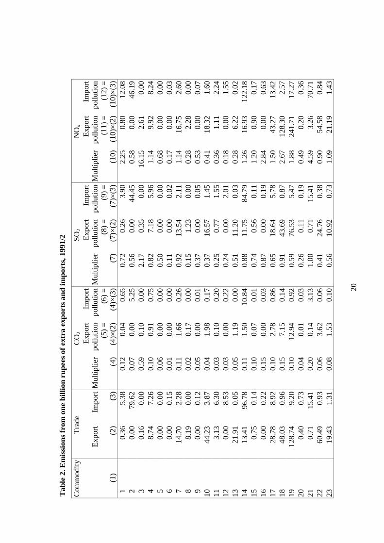
The results are given in Table 2. Using I for India, instead of S for South, columns
(2) and (3) indicate Ie∆ and Im∆ , respectively. We have calculated the extra pollution
due to an increase in trade of one billion rupees, leaving the balance on the current
account invariant. So, for example, if the actual export vector in 1991/2 is denoted by
2/1991Ie then Ie∆ = (1,000/557,166) 2/1991
Ie , where the 557,166 is the total amount of
exports (in mrs) in 1991/2. The vector Ie∆ in column (2) gives the extra exports (in mrs)
of each commodity if total exports increase by one billion rupees. Note that the vector
reflects the shares of each commodity in the actual exports of 1991/2 (i.e. division by 10
gives the percentage contribution to total exports of each commodity).
Insert Table 2. Emissions from one billion extra exports and imports, 1991/2
The multipliers in column (4) are given by the elements of the vector II Lγ′ and
indicate the emission of CO2 (in thousand tons) that is required per mrs of final demand
of commodity j. Multiplying, for commodity j, the multiplier with the extra exports gives
the extra pollution in column (5), which corresponds to the row vector )ˆ( III eL ∆′γ .
The most important conclusion from Table 2 (and Table A2 in the Appendix, for
1996/7) is that India cannot be characterized as a pollution haven. The idea was that an
increase of trade implies extra pollution because exports increase, but less pollution
because imports increase (which are no longer produced at home anymore). For a
pollution haven, the first effect is larger than the second effect, so that there will be a net
increase in pollution. Pollution havens export “dirty” products and import relatively
“clean” products. It is clear from the totals in Table 2 that the import related pollution is
much larger than the export related pollution in India, so that India gains (in terms of
emissions) from trade. Note that for a country to be characterized as a pollution haven, it
was necessary that the country itself loses from trade, while its trading partner (RoW in

10
the present case) gains. The pollution haven hypothesis can thus be accepted only if both
requirements are fulfilled (i.e. 0>∆=∆ IS ππ and 0<∆=∆ RoWN ππ ). Because input-
output data for the RoW are lacking, it is not possible to fully test the pollution haven
hypothesis. For its rejection, however, it suffices if one of the two requirements fails to be
met, as is the case for India, with total export pollution being substantially smaller than
total import pollution.
The developments over time strengthen this conclusion. Not only are the Indian
exports cleaner than the goods that are replaced by imports, also trade liberalization in
India has led to a further increase of its gains. To this end, we have calculated the ratio of
the export to the import related pollution (which should be larger than one for a pollution
haven). Together with the volumes of total exports and imports, they are listed in Table 3.
The results show that an increase of the imports reduces the pollution roughly by twice as
much as the increase of the exports (by the same amount) raises the pollution in India.
Moreover, the gains of extra trade have clearly increased over time. So, India was not a
pollution haven in the early 1990s and has moved even further away from being a
pollution haven.
Insert Table 3. Ratios of export to import pollution
Closer inspection of the results in Table 2 shows that the five most important
export commodities (Other Services, commodity 43; Other Textiles, 19; Trade, 42; Other
Manufacturing, 38; and Rail and Other Transport Services, 40) cover 56% of all exports.
In the same way we find that 55% of all imports are concentrated in the top five
commodities (Agricultural and Other Non-electrical Machinery, 33; Other Chemicals, 28;
Metals and Non-metallic Minerals, 14; Rail and Other Transport Services, 40; and Crude
Petroleum and Natural Gas, 2). The three largest multipliers are found for Electricity
(commodity 3), Petroleum Products (25) and Fertilizers (26) in case of CO2 and SO2, and
for Electricity (3), Cement (29) and Iron and Steel (31) in case of NOx. Most of the
largest differences between import related pollution and export related pollution
obviously correspond with commodities with a large multiplier and/or a large difference
between import and export share. The most notable commodity in this respect is

11
Petroleum Products (25), having the sixth largest import share, a minor export share and
outstanding multipliers (by far the largest in case of CO2 and SO2, and the fourth largest
for NOx).
It should be emphasized that our analysis is based on the assumption that all the
fossil fuels (coal, crude oil and natural gas) are combusted in producing the final
demands. That is, in producing the commodities that are used for private and government
consumption, that are used as investment goods and that are exported. So, not the final
use of the commodities itself generates the emissions, but their production. For almost all
commodities this seems to be a plausible assumption, except for commodities such as
Petroleum Products. For these products one might argue that combustion takes place
when they are actually consumed (either at home as part of private consumption or
abroad as part of foreign consumption, which is included in the Indian exports). In
particular because Petroleum Products were responsible for a substantial part of the
differences between import and export related pollution, it seems reasonable to check to
what extent our findings stem from the assumption we have made.
Let us suppose that, in contrast to our earlier assumption, combustion and thus
pollution takes place only when the final commodity is used (e.g. consumed). This
alternative assumption is made for the following three commodities: Coal and Lignite (1),
Crude Petroleum and Natural Gas (2), and Petroleum Products (25). As a consequence,
any increase in the exports of these commodities does not change the pollution in India,
because pollution takes place abroad when the products are combusted. In the same way,
an increase of the imports leaves the pollution in India unchanged. Combustion and
pollution take place in India, no matter whether the commodities are imported or
produced at home. This affects the results in Table 2, in the sense that both the export and
the import related pollution have to be set at zero, for each of the three commodities. The
new column totals and ratios under this alternative assumption are given in Table 4.
Insert Table 4. Emission results under the alternative assumption
The major conclusion to be drawn from Table 4, is that the alternative assumption
does not change our central finding. That is, India was not a pollution haven in 1991/2
12
and showed a tendency over time of increasing gains from trade. Of course, both the
export and the import related pollution have been reduced by adopting the alternative
assumption. For the three listed commodities, an increase of trade doesn’t affect pollution
under this alternative, because it no longer matters where production has taken place. It is
the final consumption that causes fossil fuel combustion and thus pollution, not the
production of these commodities (as was the case under the original assumption). As
became already clear in Table 2, the alternative assumption decreases import related
pollution much more than it does reduce export related pollution. As a consequence, the
ratio of export to import related pollution increases substantially, exports being only some
25% less polluting than imports, instead of the 50% in Table 2. Also the tendency for the
ratio to decrease (i.e. moving further away from being a pollution haven) has diminished.
Yet, the ratios are still significantly smaller than one and they still do exhibit a decline
over time.
The results sketched by our empirical findings seem to be fairly robust. First, it
should be mentioned that in reality none of the two assumptions will be exactly true.
Solving this problem would require that for each of the three commodities it would have
to be estimated what percentage of pollution is caused by its production and what
percentage is caused by its final consumption. If that information were available, the
corresponding export to import related pollution ratios would obviously be smaller than
those in Table 4 but larger than those in Table 3. So, the conclusion of India not being a
pollution haven during the 1990s would have been unchanged. Second, even if the
alternative assumption had been taken into account also for some other commodities, the
conclusions would not have been affected. As we have seen in Table 2, the gap between
import and export related pollution was (for CO2 and SO2) by far the largest for
Petroleum Products (commodity 25). Precisely this commodity was involved in the
alternative assumption. Including other commodities will affect the numerical outcomes,
but to a much lesser and to a more balanced extent.
5. Conclusions

13
In this paper we have examined the pollution haven hypothesis for India. The hypothesis
expresses that, because the pollution regulations are stronger or the restrictions on
emissions are tighter in developed countries than in developing countries, the latter will
export “dirty” products and import “clean” products. We have calculated by how much
the pollution – i.e. CO2, SO2 and NOx emissions – in India will increase if exports are
raised by one billion rupees, using the actual share of each commodity in total exports. In
the same way, it was calculated by how much Indian pollution will fall due to an increase
of its imports by one billion rupees (using the actual commodity shares in total imports).
The emissions will be reduced because the imported goods do no longer need to be
produced domestically. The effects of this one billion rupees of extra trade on the
emissions are obtained from calculating the coal, oil and natural gas embodied in each
commodity. Here we have used the assumption that these requirements of fossil fuels are
entirely combusted somewhere in the production processes.
The results showed that the increase in pollution caused by the extra exports is
much smaller (roughly half the size) than the decrease in pollution due to extra imports.
So, in terms of pollution, India gains from extra trade. According to the pollution haven
hypothesis, we would expect that a developing country loses from extra trade, while its
trading partner gains. Our findings clearly indicate that the pollution haven hypothesis
should be rejected in the case of India. The results also showed that during the 1990s –
when trade roughly doubled in India – the gains from trade even increased further,
indicating that there is no tendency to move towards becoming a pollution haven.
About fifty years ago, Leontief (1953, 1956) carried out almost the same exercise
to empirically test the Heckscher-Ohlin (HO) theory and found similar surprising results.
In its simplest form – with two countries, two goods, and two factors (labor and capital) –
the HO model predicts that the relatively labor abundant country will export the good that
is produced relatively labor intensive and will import the relatively capital intensive good.
Leontief calculated that the – direct and indirect – labor and capital requirements
necessary to satisfy $1 million of extra exports, were 182.3 worker years and $2.6 million
of capital. Replacing a reduction of domestic output by extra imports (to the amount of $1
million) would decrease the requirements by 170.0 worker years and $3.1 million of
capital. The US, commonly believed to be the most capital abundant country at that time,

14
was thus found to export labor intensive goods and to import capital intensive goods,
however. This result has become known as the Leontief paradox and still continues to
trigger ample scientific research.
Although we have focused on emissions instead of on the labor and capital
content of imports and exports, our results show a striking resemblance to Leontief’s.
Upon closer inspection, it appears that we may even view our analysis from a HO
perspective. In an attempt to reconcile Leontief’s findings, it has been suggested to
include natural resources as a third factor (see, for example, Leamer, 1980, 1984). In our
case, it may be argued that “emission permits” play a role as a third factor. Developing
countries are commonly believed to be relatively well endowed with emission permits,
for various reasons. For example, in developing countries, governments have different
priorities and set lower environmental standards, there is more room left for output
expansion before the limits are reached, less monitoring and enforcements of regulations
take place, and the size of the informal sector in the economy is larger. We would thus
expect developing countries to be relatively abundant in emission permits and, according
to the HO theory, to have a comparative advantage in (and therefore export) relatively
emission intensive goods. This outcome is exactly what is hypothesized for a pollution
haven. The pollution haven hypothesis may thus be viewed as a result of the HO model.7
It should be mentioned that there is one difference between the assumptions
underlying Leontief’s analysis and ours. Instead of calculating the foreign factor content
of US imports on the basis of the foreign input matrix, Leontief estimated this factor
content by computing the US factor content (i.e. using the US input matrix) of the
domestic production that would replace the US imports. Although, Leontief may have
been forced to do so because of a lack of data, the procedure is in line with the HO
model. In the HO theory, the assumption is made that both trading partners have access to
the same technologies. If the factor prices are equalized across countries, this implies that
the labor and capital content of US imports can be calculated by using a single – for
example the US – input matrix. Recent modifications of the HO model account for
technological differences (see, for example, Trefler, 1993, 1995; Harrigan, 1997). Note
7 It should be stressed that we have only partially tested the pollution haven hypothesis. Testing the HOtheory in a multifactor framework would require additional labor and capital data, which are not available.

15
that our calculations did not require an explicit assumption and thus allowed for different
technologies. The foreign factor (in our case emissions) content of the Indian imports
simply is not involved in our analysis. In examining the pollution haven hypothesis, we
were interested in the Indian emission content of the domestically produced commodities
that are substituted by imported goods, because this substitution reduces production and
therefore pollution in India. We have thus not used this Indian emission content to
estimate the foreign emission content, which would have required the assumption of
identical technologies.
Summarized, given that the pollution haven hypothesis can be viewed as a result
of the HO theory, and given that the hypothesis was rejected for India, it seems that this
gives rise to a green Leontief paradox. Further empirical studies for other (developing)
countries should indicate whether India is an exception or whether the Indian results hint
at a general phenomenon. It should be mentioned that – due to data limitations – we have
only been able to take a small number of environmental indicators into account. For
example, it may well be that the outcome is different if indicators for water pollution are
considered.
A possible explanation for the results, might be given by the factor endowment
hypothesis, which offers another view on the impact of international trade on the
allocation of environmental burdens across countries. This hypothesis maintains that
pollution intensities of production are highly correlated with capital intensities (see e.g.
Copeland and Taylor, 2003). In that case, capital-abundant countries (i.e. typically rich,
developed countries) have a comparative advantage in pollution intensive goods, which
they will export according to the HO theory. A lack of sectoral capital-stock data for
India, however, prevents us from further empirically investigating this alternative
hypothesis. Yet, the results seem to be more in line with the factor endowment hypothesis
than with the pollution haven hypothesis.
16
References
Antweiler, W. (1996) The Pollution Terms of Trade, Economic Systems Research, 8, pp.
361-365.
Copeland, B.R. and M.S. Taylor (2003) Trade and the Environment: Theory and
Evidence (Princeton, Princeton University Press).
Daly, H. (1993) Problems with Free Trade: Neoclassical and Steady-State Perspectives,
in: D. Zaelke, P. Orbuch, and R.F. Housman (eds) Trade and Environment: Law,
Economics and Policy (Washington, DC, Island Press), pp. 147-157.
Eskeland, G.S. and A.E. Harrison (2003) Moving to Greener Pastures? Multinationals
and the Pollution Haven Hypothesis, Journal of Development Economics, 70, pp.
1-23.
Fieleke, N.S. (1974) The Energy Content of US Exports and Imports, International
Finance Discussion Papers, no. 51 (Washington, DC, Board of Governors of the
Federal Reserve System).
Harrigan, J. (1997) Technology, Factor Supplies, and International Specialization:
Estimating the Neoclassical Model, American Economic Review, 87, pp. 475-494.
Jones, T. (1998) Economic Globalisation and the Environment: An Overview of the
Linkages, in: OECD, Globalisation and the Environment: Perspectives from
OECD and Dynamic Non Member Economies (Paris, OECD), pp. 17-28.
Kraines, S. and Y. Yoshida (2004) Process System Modeling of Production Technology
Alternatives using Input-Output Tables with Sector Specific Units, Economic
Systems Research, 16, pp. 23-34.
Leamer, E.E. (1980) The Leontief Paradox, Reconsidered, Journal of Political Economy,
88, pp. 495-503.
Leamer, E.E. (1984) Sources of International Comparative Advantage: Theory and
Evidence (Boston, MIT Press).
Lenzen, M. (2001) A Generalized Input-Output Multiplier Calculus for Australia,
Economic Systems Research, 13, pp. 65-92.

17
Leontief, W. (1953) Domestic Production and Foreign Trade; The American Capital
Position Re-examined, Proceedings of the American Philosophical Society, 97,
pp. 332-349.
Leontief, W. (1956) Factor Proportions and the Structure of American Trade: Further
Theoretical and Empirical Analysis, Review of Economics and Statistics, 38, pp.
386-407.
Machado, G., R. Schaeffer and E. Worrell (2001) Energy and Carbon Embodied in the
International Trade of Brazil: An Input-Output Approach, Ecological Economics,
39, pp. 409-424.
Miller, R.E. and P.D. Blair (1985) Input-Output Analysis: Foundations and Extensions
(Englewood Cliffs, NJ, Prentice Hall).
Munksgaard, J. and K.A. Pedersen (2001) CO2 Accounts for Open Economies: Producer
or Consumer Responsibility?, Energy Policy, 29, pp. 327-334.
Nordström, H. and S. Vaughan (1999) Trade and Environment, Special Studies, no. 4
(Geneva, WTO).
OECD (1997) Economic Globalisation and the Environment (Paris, OECD).
Pearce, D.W. and J.J. Warford (1993) World Without End: Economics, Environment and
Sustainable Development (New York, Oxford University Press).
Planning Commission (1995) A Technical Note to the Eighth Plan of India, Input-Output
Transaction Table for 1991-92 (New Delhi, Government of India).
Planning Commission (2000) Input-Output Transaction Table For 1996-97 (New Delhi,
Government of India).
Proops, J.L.R., G. Atkinson, B. Frhr. v. Schlotheim and S. Simon (1999) International
Trade and the Sustainability Footprint: A Practical Criterion for its Assessment,
Ecological Economics, 28, pp. 75-97.
Trefler, D. (1993) International Factor Price Differences: Leontief was Right!, Journal of
Political Economy, 101, pp. 961-987.
Trefler, D. (1995) The Case of Missing Trade and Other Mysteries, American Economic
Review, 85, pp. 1029-1046.
UNFCCC (1992) United Nations Framework Convention on Climate Change (New
York, UN).

18
Wyckoff, A.W. and J.M. Roop (1994) The Embodiment of Carbon in Imports of
Manufactured Products: Implications for International Agreements on Greenhouse
Gas Emissions, Energy Policy, 22, pp. 187-194.
Wright, D.J. (1974) Goods and Services: An Input-Output Analysis, Energy Policy, 2, pp.
307-315.

19
Table 1. Conversion factors
Emissions in million tons1991/2 CO2 SO2 NOx
Combustion of one mrs of: coal & lignite crude petroleum & natural gas
c1 = 5.1376c2 = 3.1548
× 10-3
s1 = 0.0156s2 = 0.0330
n1 = 0.1534n2 = 0.0033
1996/7Combustion of one mrs of: coal & lignite crude petroleum & natural gas
c1 = 4.9143c2 = 2.2944
× 10-3
s1 = 0.0149s2 = 0.0240
n1 = 0.1467n2 = 0.0024
20
Tab
le2.
Em
issi
ons
from
one
billi
onru
pees
ofex
tra
expo
rts
and
impo
rts,
1991
/2
Com
mod
ityT
rade
CO
2SO
2N
Ox
(1)
Exp
ort
(2)
Impo
rt (3)
Mul
tiplie
r
(4)
Exp
ort
pollu
tion
(5)
=(4
)×(2
)
Impo
rtpo
lluti
on(6
)=
(4)×
(3)
Mul
tiplie
r
(7)
Exp
ort
pollu
tion
(8)
=(7
)×(2
)
Impo
rtpo
lluti
on(9
)=
(7)×
(3)
Mul
tiplie
r
(10)
Exp
ort
pollu
tion
(11)
=(1
0)×
(2)
Impo
rtpo
lluti
on(1
2)=
(10)
×(3
)1
0.36
5.38
0.12
0.04
0.65
0.72
0.26
3.90
2.25
0.80
12.0
82
0.00
79.6
20.
070.
005.
250.
560.
0044
.45
0.58
0.00
46.1
93
0.16
0.00
0.59
0.10
0.00
2.17
0.35
0.00
16.1
52.
610.
004
8.74
7.26
0.10
0.91
0.75
0.82
7.18
5.96
1.14
9.92
8.24
50.
000.
000.
060.
000.
000.
500.
000.
000.
680.
000.
006
0.00
0.15
0.01
0.00
0.00
0.11
0.00
0.02
0.17
0.00
0.03
714
.70
2.28
0.11
1.66
0.26
0.92
13.5
42.
111.
1416
.75
2.60
88.
190.
000.
020.
170.
000.
151.
230.
000.
282.
280.
009
0.00
0.12
0.05
0.00
0.01
0.37
0.00
0.05
0.53
0.00
0.07
1044
.23
3.87
0.04
1.98
0.17
0.37
16.5
71.
450.
4118
.32
1.60
113.
136.
300.
030.
100.
200.
250.
771.
550.
361.
112.
2412
0.00
8.53
0.03
0.00
0.22
0.24
0.00
2.01
0.18
0.00
1.55
1321
.91
0.05
0.05
1.19
0.00
0.51
11.2
00.
030.
286.
220.
0214
13.4
196
.78
0.11
1.50
10.8
40.
8811
.75
84.7
91.
2616
.93
122.
1815
0.75
0.14
0.10
0.07
0.01
0.74
0.56
0.11
1.20
0.90
0.17
160.
000.
220.
150.
000.
030.
870.
000.
192.
840.
000.
6317
28.7
88.
920.
102.
780.
860.
6518
.64
5.78
1.50
43.2
713
.42
1848
.03
0.96
0.15
7.15
0.14
0.91
43.6
90.
872.
6712
8.30
2.57
1912
8.74
9.20
0.10
12.9
40.
920.
5976
.53
5.47
1.88
241.
7117
.27
200.
400.
730.
040.
010.
030.
260.
110.
190.
490.
200.
3621
0.71
15.4
10.
200.
143.
131.
000.
7115
.41
4.59
3.26
70.7
122
60.4
90.
930.
063.
620.
060.
4124
.76
0.38
0.90
54.5
80.
8423
19.4
31.
310.
081.
530.
100.
5610
.92
0.73
1.09
21.1
91.
43

21
244.
191.
450.
060.
230.
080.
381.
600.
550.
823.
421.
1825
19.6
667
.83
1.73
34.0
911
7.65
17.0
833
5.70
1158
.39
5.95
116.
9040
3.40
260.
0525
.52
0.48
0.02
12.1
83.
770.
2096
.17
5.25
0.27
133.
9027
2.15
1.92
0.08
0.17
0.15
0.56
1.20
1.07
1.11
2.38
2.13
2851
.02
107.
210.
146.
9814
.66
0.98
49.7
810
4.62
1.91
97.2
920
4.44
290.
000.
050.
360.
000.
021.
470.
000.
089.
420.
000.
5230
7.05
3.41
0.28
1.98
0.96
1.64
11.5
65.
585.
3237
.53
18.1
231
6.01
33.6
30.
352.
1111
.78
1.96
11.7
765
.82
6.99
42.0
523
5.22
322.
6017
.82
0.28
0.72
4.94
1.94
5.03
34.4
94.
0310
.49
71.8
733
31.0
917
8.73
0.13
3.90
22.4
30.
7824
.20
139.
102.
2168
.55
394.
1034
12.8
628
.75
0.10
1.30
2.91
0.66
8.53
19.0
71.
6421
.13
47.2
635
0.45
8.94
0.05
0.02
0.49
0.36
0.16
3.23
0.88
0.39
7.91
368.
5535
.53
0.06
0.54
2.25
0.42
3.57
14.8
41.
018.
6836
.06
3717
.86
47.9
90.
091.
564.
190.
5710
.20
27.4
21.
4225
.36
68.1
538
100.
0048
.87
0.12
11.5
25.
630.
6868
.35
33.4
02.
1421
4.35
104.
7539
0.00
0.00
0.12
0.00
0.00
0.75
0.00
0.00
2.19
0.00
0.00
4068
.72
85.9
50.
2215
.36
19.2
11.
9413
3.20
166.
611.
7812
2.61
153.
3541
2.04
3.48
0.03
0.06
0.10
0.19
0.39
0.67
0.46
0.93
1.59
4210
8.95
0.00
0.04
4.08
0.00
0.27
29.8
90.
000.
4953
.77
0.00
4315
4.61
54.7
40.
034.
381.
550.
1523
.91
8.47
0.58
89.6
531
.74
Tot
al10
00.0
010
00.0
012
4.92
244.
8395
7.99
2055
.02
1481
.10
2219
.88
Not
es.E
xpor
ts(2
)an
dim
port
s(3
)ar
ein
mill
ion
rupe
es(m
rs),
and
sum
toon
ebi
llion
rupe
es.M
ultip
liers
in(4
)ar
ein
thou
sand
tons
ofC
O2
per
mrs
offi
nal
dem
and
for
com
mod
ityj.
Mul
tiplie
rsin
(7)
and
(10)
are
into
nsof
SO2
and
NO
xpe
rm
rsof
fina
lde
man
d.T
hepo
lluti
onin
(5)
and
(6)
isin
thou
sand
tons
,the
pollu
tion
in(8
),(9
),(1
1)an
d(1
2)is
into
ns.

22
Table 3. Ratios of export to import pollution
1991/2 1996/7
Export to import ratios of pollution
CO2
SO2
NOx
0.51
0.47
0.67
0.42
0.38
0.57
Volumes (in 1991/2 prices) of
Exports (in mrs)
Imports (in mrs)
557,166
728,480
1,022,874
1,126,411
Table 4. Emission results under the alternative assumption
1991/2 1996/7
ExportPollution
ImportPollution Ratio
ExportPollution
ImportPollution Ratio
CO2
SO2
NOx
90.79
622.03
1363.40
121.28
848.28
1758.21
0.75
0.73
0.78
80.60
566.86
1156.26
111.76
771.36
1660.29
0.72
0.73
0.70
Note. CO2 emissions are in thousand tons, SO2 and NOx emissions in tons. The increasein total exports and imports is one billion rupees (in 1991/2 prices).

23
Table A1. Commodity classification
1 Coal and Lignite 22 Leather and Leather Products2 Crude petroleum and Natural Gas 23 Rubber products3 Electricity 24 Plastic Products4 Cereals and Pulses 25 Petroleum Products5 Sugercane 26 Fertilizers6 Jute 27 Pesticides7 Cotton 28 Other Chemicals8 Tea and Coffee 29 Cement9 Rubber 30 Other Non-metallic Mineral Products10 Other Crops 31 Iron and Steel11 Animal Husbandry 32 Nonferrous Metals12 Forestry and Logging 33 Agricultural and Other13 Fishing Non-electrical Machinery14 Metals and Non-metallic Minerals 34 Electrical Machinery15 Sugar 35 Communication Equipment16 Hydrogenated Oil 36 Electronic Equipment17 Other Food and Beverages 37 Rail and Other Transport Equipment18 Cotton Textiles 38 Other Manufacturing19 Other Textiles 39 Construction20 Wood and Wood Products 40 Rail and Other Transport Services21 Paper and Paper Products 41 Communication22 Leather and Leather Products 42 Trade23 Rubber products 43 Other Services

24
Tab
leA
2.E
mis
sion
sfr
omon
ebi
llion
rupe
esof
extr
aex
port
san
dim
port
s,19
96/7
Com
mod
ityT
rade
CO
2SO
2N
Ox
(1)
Exp
ort
(2)
Impo
rt (3)
Mul
tiplie
r
(4)
Exp
ort
pollu
tion
(5)
=(4
)×(2
)
Impo
rtpo
lluti
on(6
)=
(4)×
(3)
Mul
tiplie
r
(7)
Exp
ort
pollu
tion
(8)
=(7
)×(2
)
Impo
rtpo
lluti
on(9
)=
(7)×
(3)
Mul
tiplie
r
(10)
Exp
ort
pollu
tion
(11)
=(1
0)×
(2)
Impo
rtpo
lluti
on(1
2)=
(10)
×(3
)1
0.19
1.54
0.09
0.02
0.14
0.62
0.12
0.95
1.48
0.29
2.27
20.
0038
.96
0.06
0.00
2.39
0.47
0.00
18.3
50.
720.
0028
.15
30.
090.
440.
520.
050.
231.
880.
160.
8414
.35
1.25
6.37
47.
925.
940.
080.
640.
480.
604.
763.
571.
038.
186.
145
0.00
0.00
0.05
0.00
0.00
0.37
0.00
0.00
0.62
0.00
0.00
60.
000.
140.
010.
000.
000.
090.
000.
010.
160.
000.
027
9.63
2.01
0.09
0.85
0.18
0.68
6.56
1.37
1.03
9.96
2.08
82.
700.
000.
020.
060.
000.
140.
380.
000.
320.
860.
009
0.00
0.08
0.04
0.00
0.00
0.28
0.00
0.02
0.47
0.00
0.04
1041
.47
2.91
0.04
1.63
0.11
0.33
13.5
10.
950.
3715
.31
1.07
112.
186.
270.
030.
060.
180.
210.
461.
330.
350.
762.
1812
0.00
8.29
0.02
0.00
0.19
0.20
0.00
1.67
0.17
0.00
1.39
1317
.61
0.07
0.14
2.39
0.01
1.31
23.0
10.
100.
5910
.32
0.04
1411
.38
138.
280.
131.
4417
.44
0.99
11.2
513
6.70
1.42
16.1
119
5.77
150.
820.
440.
080.
070.
040.
640.
530.
291.
030.
850.
4616
0.00
0.20
0.15
0.00
0.03
0.91
0.00
0.18
2.56
0.00
0.52
1718
.54
10.8
70.
101.
841.
080.
7013
.05
7.65
1.39
25.8
615
.16
1848
.21
0.96
0.13
6.17
0.12
0.74
35.5
50.
702.
4711
9.08
2.36
1914
1.79
9.17
0.10
14.3
90.
930.
7410
5.38
6.81
1.34
190.
2412
.30
200.
280.
760.
030.
010.
020.
220.
060.
170.
420.
120.
3221
0.49
16.6
20.
170.
082.
760.
860.
4314
.37
3.57
1.77
59.3
422
66.2
71.
150.
053.
320.
060.
3522
.99
0.40
0.74
49.2
10.
8523
13.5
01.
270.
060.
840.
080.
466.
160.
580.
8211
.05
1.04

25
242.
910.
950.
060.
170.
050.
411.
180.
390.
822.
380.
7825
10.7
289
.26
1.19
12.7
910
6.49
11.5
712
4.01
1.03
2.28
4.80
51.4
342
8.15
260.
0524
.15
0.32
0.01
7.74
2.41
0.11
58.2
13.
990.
1896
.28
272.
621.
840.
070.
180.
130.
511.
330.
940.
942.
471.
7428
62.2
468
.34
0.14
8.87
9.74
1.05
65.3
371
.73
1.86
115.
7412
7.07
290.
530.
440.
270.
140.
121.
160.
620.
526.
783.
603.
0030
3.84
2.27
0.25
0.97
0.58
1.64
6.29
3.71
4.21
16.1
69.
5531
4.33
32.9
00.
341.
4611
.10
1.74
7.53
57.1
87.
3031
.62
240.
1532
2.07
14.7
20.
280.
584.
142.
044.
2330
.09
3.77
7.81
55.4
733
28.0
218
0.55
0.14
3.85
24.8
30.
8223
.09
148.
752.
5370
.88
456.
6434
10.8
034
.99
0.06
0.62
2.01
0.41
4.48
14.5
00.
788.
4527
.36
350.
307.
620.
060.
020.
440.
410.
123.
120.
830.
256.
3336
32.5
353
.39
0.05
1.63
2.68
0.35
11.3
018
.54
0.74
24.2
039
.71
3715
.45
42.5
70.
101.
474.
060.
609.
2525
.50
1.64
25.3
569
.88
3813
5.87
26.6
00.
0810
.30
2.02
0.46
63.0
912
.35
1.36
184.
2836
.07
390.
000.
000.
110.
000.
000.
620.
000.
002.
000.
000.
0040
56.1
010
3.14
0.16
9.03
16.6
01.
3575
.61
138.
991.
4782
.50
151.
6741
1.10
4.17
0.03
0.03
0.11
0.17
0.19
0.73
0.39
0.43
1.64
4216
9.13
0.00
0.03
5.64
0.00
0.23
38.8
60.
000.
5083
.90
0.00
4378
.30
65.7
20.
021.
781.
490.
1310
.02
8.41
0.45
35.1
629
.51
Tot
al10
00.0
010
00.0
093
.41
220.
7869
0.99
1822
.94
1207
.98
2118
.86
Not
es.E
xpor
ts(2
)an
dim
port
s(3
)ar
ein
mill
ion
rupe
es(m
rs),
and
sum
toon
ebi
llion
rupe
es.M
ultip
liers
in(4
)ar
ein
thou
sand
tons
ofC
O2
per
mrs
offi
nal
dem
and
for
com
mod
ityj.
Mul
tiplie
rsin
(7)
and
(10)
are
into
nsof
SO2
and
NO
xpe
rm
rsof
fina
lde
man
d.T
hepo
lluti
onin
(5)
and
(6)
isin
thou
sand
tons
,the
pollu
tion
in(8
),(9
),(1
1)an
d(1
2)is
into
ns.


