GREATER TORONTO AREA URBAN HEAT ISLAND: ANALYSIS OF

TEMPERATURE AND EXTREMES

by

Tanzina Mohsin

A thesis submitted in conformity with the requirements

for the Degree of Doctor of Philosophy

Graduate Department of Geography

University of Toronto

©Copyright by Tanzina Mohsin (2009)

ii

Greater Toronto Area Urban Heat Island: Analysis of Temperature and Extremes

Doctor of Philosophy (2009)

Tanzina Mohsin

Department of Geography

University of Toronto

Abstract

This study analyzes the trends in temperature, and their extremes, in the Greater

Toronto Area (GTA) in the context of urban heat island. The trends in annual and seasonal

temperature changes were investigated in the GTA over the past century and a half with

special focus on 1970-2000. The Mann-Kendall test is used to assess the significance of the

trends and the Theil-Sen slope estimator is used to identify their magnitude. Statistically

significant increasing trends for mean and minimum temperatures are observed mainly at the

urban and suburban stations. The sequential Mann-Kendall test is used to identify any abrupt

change in the time series of temperature (31 -161 years), and the results indicate that

increasing trend for annual mean temperature has started after 1920 at Toronto downtown,

after the 1960s at the suburban stations, and has increased significantly during the 1980s at

all stations, which is consistent with the pace of urbanization during these periods in the

GTA. The observed urban heat island (UHI) in Toronto is quantified and characterized by

considering three different rural stations. The UHI intensity (∆Tu-r) in Toronto is categorized

as winter dominating or summer dominating depending on the choice of a rural station. The

results from the trend analysis of annual and seasonal ∆Tu-r suggest that the choice of the

rural station is crucial in the estimation of ∆Tu-r, and thus can overestimate or underestimate

its prediction depending on the location and topographical characteristics of a rural station

iii

relative to the urban station. The trends in extreme temperature indices are also investigated

and the results indicate that indices based on daily maximum temperature are more

pronounced at the urban and suburban stations compared to that at the rural stations. The

changes in the trends for extreme indices based on daily minimum temperature are consistent

at all stations for the period of 1971-2000. With the decrease in the percentage of cold nights

and the increase in the percentage of warm nights, the diurnal temperature range has

decreased throughout the GTA region. The analysis of heating degree days and cooling

degree days revealed that the former is associated with decreasing trends and the latter

exhibited increasing trends at almost all stations in the GTA. Finally, it is evident from the

results that urban heat island phenomenon exerts warmer influence on the climate in cities,

and with the current pace of urbanization in the GTA, it is imperative to understand the

potential impact of the emerging UHI on humans and society.

iv

Acknowledgements

I wish to acknowledge the financial support from the Government of Ontario Graduate

Scholarship (OGS), Ontario Graduate Scholarship in Science and Technology, and the

George Tatham/Geography Alumni Graduate Scholarship. I also wish to thank Maria Petrou,

Climate Services in Environment Canada for data and information without which some part

of this research project would have been incomplete. Special acknowledgements to Vincent

Cheng, GIS specialist, Environment Canada, for his suggestions on the GIS figures. A

special thanks to my husband, Ehsan-ul Quayyum and my two children, for their support

throughout the completion of this dissertation. Finally, many thanks to my supervisor,

William A. Gough for his constant guidance and motivation without which this research

project would have not been possible. Also, many thanks to my supervisory committee:

David Etkin, Scott Munro and Sarah Finkelstein for their suggestions towards the completion

of this dissertation.

v

TABLE OF CONTENTS

CHAPTER 1: INTRODUCTION 1

1.1: Background and rationale 1

1.2 Objectives 9

CHAPTER 2: TREND ANALYSIS OF LONG TERM TEMPERATURE TIME SERIES IN THE GREATER TORONTO AREA (GTA) 12

2.1 Introduction 12

2.2 Data and Analysis 15

2.3 Results and Discussion 22

2.4. Conclusions 44

CHAPTER 3: CHARACTERIZATION OF TORONTO’S URBAN HEAT ISLAND: IMPACT OF SELECTION OF RURAL SITES 47

3.1. Introduction 47

3.2. Data and Methodology 50

3.3. Results and discussion 55

3.4 Summary and Conclusions 78

vi

CHAPTER 4: ANALYSIS OF TRENDS FOR EXTREMES INDICES OF DAILY OBSERVED TEMPERATURE IN THE GREATER TORONTO AREA (GTA) 80

4.1. Introduction 80

4.2. Data and methodologies 83

4.3. Results and discussion 88

4.4 Summary and conclusions 118

CHAPTER 5: DISCUSSION AND CONCLUSIONS 121

REFERENCES 128

APPENDIX 144

LIST OF ACRONYMS 146

vii

List of Figures Figure 1.1 The growth of the build up areas in Toronto, 1861-1941. 3

Figure 1.2 Population change in Toronto census metropolitan area for the period of 1986-

2006. 4

Figure 1.3 Comparison of population density at Toronto and its surrounding areas between

1971 and 2001. 5

Figure 1.4 Idealized illustrations of a typical lake breeze circulation and its associated front.

Common features are labeled. The dashed line represents the outer boundary of the

inflow layer (Sills, 1998). 7

Figure 2. 1 Map showing the locations of the meteorological stations in the GTA. 17

Figure 2.2 Statistical time series of annual maximum, minimum and mean temperatures. 23

Figure 2.3 Abrupt changes in climate for annual mean temperature for the stations in the

GTA. (the test statistics from sequential Mann-Kendall test for forward and backward

time series are plotted to detect the abrupt changes). 33

Figure 2.4 Comparison of trends for the statistical time series of annual temperatures for

Toronto and Beatrice as derived from the sequential Mann-Kendall test. (Test sample

values are shown corresponding to the temperature time series for each year). 36

Figure 2.5 Comparison of the changes in annual maximum, minimum and mean temperature

between two periods, 1970-2000 and 1989-2000, at the stations in the GTA with

increasing distance from Toronto downtown. 41

Figure 2.6 Spatial patterns of annual temperature changes for the period of 1989-2000 and

1970-2000. Figures on the left are based on 12 years annual average and figures on the

viii

right are based on 31 years annual average for the annual maximum, minimum and

mean temperatures respectively (top to bottom). 43

Figure 3.1 Locations of the meteorological stations used in the analysis. 52

Figure 3.2 Year-to-year variation of UHI intensity at Toronto and Pearson with three rural

stations for the period of 1970-2000. 58

Figure 3.3 Monthly mean changes of urban-rural temperature difference at Toronto and

Pearson with three different rural stations for the period of 1970-2000. 63

Figure 3.4 Seasonal changes in ∆Tu-r at Toronto and at Pearson for three different rural

stations for the period of 1970-2000. 66

Figure 3.5 Frequency of intensity of UHI at Toronto and at Pearson for three different rural

stations for the period of 1970-2000. 68

Figure 3.6 Change in the amplitude of UHI intensity at Toronto and Pearson in relation to

wind speed for July and February, 2006. 73

Figure 3.7 Comparison of the diurnal variation of UHI intensity in July and February

between Toronto and Pearson. 74

Figure 3.8 Diurnal changes in UHI intensity at Toronto and Pearson on July (02-03) and

February (09-10), 2006;(the bars are proportional to the magnitude of UHI intensity). 77

Figure 4. 1 Map showing the stations used for extreme temperature analysis in the GTA. 84

Figure 4.2 Spatial distribution of hot days, summer days, ice days and frost days in the GTA.

The circles are proportional to the magnitude of the average number of days for the

ix

period of 1971-2000. The average number of days per year is indicated inside the

circles. 93

Figure 4. 3 (a) Trends in indices based of daily maximum temperature (hot days, summer

days, warmest days, warm days, cold days and ice days) for the period of 1971-2000. 99

Figure 4.3 (b) Same as 4.3a, only for indices based on daily minimum temperature. 102

Figure 4.3 (c) Same as 4.3a, only for the indices based on both maximum and minimum

temperatures (diurnal temperature range and extreme temperature range). 103

Figure 4.4 Extreme temperature indices for seasonal temperature time series for the GTA.

The linear trend is shown by the bold line. A) Warm Days, B) Warm Nights, C) Cold

Days and D) Cold Nights. 110

Figure 4.5 Comparison of the changes in heating degree days (HDD) and cooling degree

days (CDD) for two different periods, 1971-2000 and 1991-2000. 113

Figure 4. 6 (a) Spatial comparison of the changes in HDD between 1971-2000 and 1991-

2000 (positive sign indicates increasing trend and negative sign indicates negative

trends). 116

Figure 4.6 (b) Spatial comparison of the changes in CDD between 1971-2000 and 1991-2000

(positive sign indicates increasing trend and negative sign indicates negative trends). 117

x

List of Tables

Table 2.1 Meteorological stations in the GTA. 16

Table 2.2 The autocorrelation coefficients for lags 1, 2 and 3 for the period of 1970 - 2000 20

Table 2.3 The u(t) test statistic and p-values from the sequential Mann-Kendall test and the

statistical significance of the trend in terms of p-values. 24

Table 2.4 The magnitude of the trend computed using the Kendall’s tau and TSA (1970-

2000). 25

Table 2.5 The seasonal trends in temperature for the period of 1970-2000 (The numbers in

the table indicate the Theil Slope estimate in °C/year. *** Significant at 99%, **

Significant at 95%, * Significant at 90%). 28

Table 2.6 The beginning of the annual and seasonal abrupt change for all stations in the GTA

(‘+’ indicates increasing trend and ‘–’ indicates decreasing trend, ‘-----’ indicates no

trend is detected). 31

Table 3.1 Results from the correlation analysis between ΔTu-r and Tr. 56

Table 3.2 Correlation between the trends of ΔTu-r and Tr. 57

Table 3.3 Estimated trends of annual UHI intensity for Toronto using Mann-Kendall test. 60

Table 3.4 Estimated trends of annual UHI intensity for Pearson using Mann-Kendall test. 60

Table 3.5 Estimated trends for seasonal ∆Tu-r for Toronto using Mann-Kendall test

(°C/decade). 70

xi

Table 3.6 Mann-Kendall test results from trend analysis of seasonal ∆Tu-r for Pearson

(°C/decade). 70

Table 4.1 Meteorological stations in the Greater Toronto Area (GTA) 84

Table 4.2 Definition of the indices in terms of daily maximum (Tmax) and minimum (Tmin)

temperature. 86

Table 4.3 Averages of the indices values over 1971-2000 for nine stations in the GTA. 89

Table 4.4 Estimated trends for the annual extreme temperature indices for the period of 1971-

2000 from the TSA analysis indicating the significant positive (+) and negative (−)

trends in the GTA (no trend indicate an estimated slope of “0”). 96

Table 4.5 Estimated trends for the seasonal extreme temperature indices from the TSA

analysis indicating the significant positive (+) and negative (−) trends in the GTA (no

trend indicate an estimated slope of “0”)* Significant at 95% 105

Table 4.6 Comparison of the trends for HDD and CDD between 1971-2000 and 1990-2000

as derived from Theil-Sen slope estimator (degree days/year). 114

1

Chapter 1: Introduction

1.1: Background and rationale A major premise of much current research in climatology is that changes in global

climate result from anthropogenic activities. Urbanization is one of the foremost

anthropogenic changes and is spreading throughout the world at an unprecedented pace. By

the end of this century a majority of the world’s population will be living in urban

environments (Camilloni and Barros, 1997; UNFPA, 1999). The urbanization process can

increase local temperature in comparison to less built up suburban/rural areas, creating an

urban heat island (UHI). An important aspect of this UHI phenomenon is its impact on local

climate change and variability. In addition, climate change caused by anthropogenic emission

of greenhouse gases is intensified by the temporal pattern and spatial extent of the UHI in

metropolitan regions. Observations of atmospheric processes in cities are thus fundamental to

advances in the understanding of climate change, especially at the local scale. According to

the Intergovernmental Panel on Climate Change (IPCC), the global mean surface-air

temperature has increased by about 0.74ºC over the past century (1906 to 2005), with

pronounced warming during the past 25 years. The urban warming component to this

measurement of temperature change is estimated to be 0.006ºC/decade since 1900 (Trenberth

et al., 2007) which is about 10% of the total warming.

Debate about the impact of urbanization on climate variables (e.g. temperature,

precipitation) has motivated many studies designed to detect trends in climate data for a

number of urban areas around the world. These studies have quantified various aspects of

2

urban-to-rural temperature differences (Munn et al. 1969; Oke, 1973; Oke and Maxwell,

1975; Oke, 1979; Oke, 1982; Oke, 1987; Camilloni and Barros, 1997; Runnalls and Oke,

2000; Çiçek and Doğan, 2006). The studies by Oke have identified important factors, which

are responsible for the difference in temperature between urban settings and their

surrounding areas, and these can be summarized as increased desertion of short-wave

radiation due to canyon geometry, decreased long wave radiation loss because of the

reduction of the sky-view factor, anthropogenic heat sources, increased sensible heat storage

and decreased evaporation due to concrete materials, and decreased total turbulent heat

transport due to wind speed reduction caused by canyon geometry. Much of the work on the

UHI has also focussed on quantifying the effect of increasing levels of urbanization in major

cities on seasonal and annual mean temperatures (Canyon and Douglas, 1984; Duchon, 1986;

Karl et al., 1988; Kadioğlu, 1997; Jauregui, 1997; Tayanc and Toros, 1997; Böhm 1998;

Philandras et al., 1999; Böhm et al., 2001,; Mihalakakouet al., 2004; Çiçek and Doğa, 2006;

Stone, 2007). These studies have demonstrated the importance of considering the influence

of urbanization in the detection of climate change, and showed how the UHI affects the

diurnal, seasonal and annual temperature changes at a local scale. For example, in the city of

Ankara, Turkey, the effect of the UHI on diurnal temperature variation is more pronounced

in winter compared to the other seasons (Çiçek and Doğa, 2006). A more recent study on the

UHI effect on the urban and rural temperature trends of several American cities suggested

that there is a clear division in temperature trends between stations situated in the cities

compared to those located in the countryside during the period from 1951 to 2000 (Stone Jr.,

2007).

This thesis identifies and analyzes the effects of urbanization on local climate

change using the city of Toronto as a case study. Toronto is one of the fastest growing urban

3

areas in North America with a population of 2.5 million (Statistics Canada, 2006). The city of

Toronto is growing since 1861 not only in terms of population, but also the housings,

constructions and industries are expanding, particularly after 1920. Figure 1.1 shows the

extent of the build up areas from 1861 to 1941, which is a major indicator of the intensity of

urbanization during that period. It can be observed from the figure that the major expansion

in the city center occurred from 1901 to 1920, after which the build up areas extended away

from the city center and continued to grow since then.

Figure 1. 1The growth of the build up areas in Toronto, 1861-1941 (Source: Harris and Lymes, 1990)

Another major indicator of urbanization, the population growth, is shown in Figure

1.2 for the Toronto census metropolitan area (CMA) during 1986-2006. A major segment of

4

this population is international immigrants because the city of Toronto welcomes almost two

thirds of the total new immigrants entering Canada every year. In addition to the immigrants,

increasing numbers of people are inclined to settle in urban areas compared to rural areas.

Therefore, urbanization in Toronto has taken a new perspective with these additions to the

population of Toronto each year, affecting its geography and climate.

2.0

2.5

3.0

3.5

4.0

4.5

5.0

5.5

6.0

1986 1988 1990 1992 1994 1996 1998 2000 2002 2004 2006

Years

Popu

latio

n in

mill

ion

Figure 1.2 Population change in Toronto census metropolitan area for the period of 1986-2006

The change in population is also evident in areas surrounding the city of Toronto, particularly

for the period of 1970 to 2000, which is the major period of focus for the analysis in this

dissertation. Figure 1.3 compares the changes in population in Toronto and its surrounding

areas between the year 1971 and 2001 (Statistics Canada, 2006).

5

Figure 1.3 Comparison of population density at Toronto and its surrounding areas between 1971 and 2001

6

The increase in population from 1971 to 2001 is apparent from Figure 1.3, which

shows that the population density has increased substantially in the suburban areas, primarily

towards north, northwest, southwest, west and east of the city core. With significant increases

in population each year (4%/yr since 1996) and its associated rapid urbanization, Toronto is

an ideal subject with which to examine the climate impact of such changes. Toronto is

situated near 44º N and on the shore of one of the Laurentian Great Lakes (Lake Ontario). As

such, Toronto’s climate results from local, regional and larger scale influences and from the

city’s UHI. The UHI in Toronto results from the urban reduction of evapotranspiration (due

to pavement and less vegetation), heat storage in buildings and pavements, artificial

generation of heat and snow removal (reduction of albedo) (Gough and Rozanov, 2001). This

UHI is expected to influence the day to day weather patterns, the seasonal temperature

changes, and even extreme climate changes at Toronto. Given that the current pace of

urbanization, it is, therefore, imperative to consider the urbanization impacts on future

changes of temperature and their extremes. It is, thus, timely to study the impact of

urbanization on climate change detection, essentially at local scales.

There is also increasing evidence that cities that are situated near large water bodies

can influence the local weather through complex urban land use-weather-climate feedbacks

(Kusaka et al., 2000). At the local scale, the climate of Toronto is affected by topography

with a change in elevation of 275 m within 35 km of the shore of Lake Ontario, which may

produce slope winds at night or subsidence heating when there is a strong northeast

temperature gradient (Munn et al, 1969). Regionally, Lake Ontario and the other Great lakes

have a modifying influence on Toronto’s climate. Regional winds, blowing from water to

land, will moderate the temperature extremes (Scott and Huff, 1996), which is known as the

“lake breeze” effect. During the day air over land expands more rapidly than air over water

7

due to the warmer underlying surface. This results in lower pressure over land than over

water, which induces a flow from water towards land at the surface known as the 'lake

breeze'. A typical lake breeze circulation and its associated front are illustrated in Figure 1.4.

The lake breeze that are initiated by Great Lakes have a typical maximum inflow wind speed

of 4-7 m/s and a little weaker maximum return flow of 2-5 m/s aloft. The maximum depth of

a typical inflow layer is between 500m and 1000m with the return flow extending to 1000m

to 2000m above the inflow layer (Moraz, 1967; Lyons, 1972; Keen and Lyons, 1978).

Figure 1.4 Idealized illustrations of a typical lake breeze circulation and its associated front. Common features are labeled. The dashed line represents the outer boundary of the inflow layer (Sills, 1998).

The onshore lake breeze wind near the surface delivers cool, moist air to locations at and

near the lake, particularly in spring and summer. The penetration distances of lake breeze for

Great Lakes regions have been reported to be near 30 km (Atkinson, 1981). The intensity of

8

lake breeze is directly proportional to the horizontal temperature gradient (Pielke and Segal,

1986). A sensitivity study on the effect of air temperature related to lake-land breeze

formation showed that the temperature of the land has more impact compared to the water

surface temperature on the formation of lake breeze. It was found that the water surface

temperature have little effect on the simulated lake breeze as long as the water surface is cool

enough to stably stratify the atmosphere over the lake (Arritt, 1987). Therefore, an area with

enhanced land temperature than water will facilitate the formation of lake breeze compared

to an area with low land temperature. Toronto, with a well defined UHI, exhibits high land

temperature during the day and in summer, and thus, the lake breeze is initiated fairly easily

with strong temperature gradient between lake and land, which generates a mitigating effect

on its temperature change and also on the changes in extremes.

One of the most serious challenges in coping with a changing climate is the changes

in extreme weather and climate events. Research suggests that changes in extremes are

already having impacts on socioeconomic and natural systems. With continued

anthropogenic activities and the associated warming, future climate change will present

additional challenges on the adaptation capability. For example, more frequent extreme

events occurring over a shorter period of time will cause the adaptation due to the impacts of

the extremes difficult. It is observed that the temperature extremes are more pronounced for

the time series of the recent years. Most of North America is experiencing more hot days and

nights during the six of the last ten years (1998-2007) (Peterson el al., 2008). The number of

heat waves also has been increasing over the past fifty years (Trenberth et al., 2007). Certain

aspects of observed increases in temperature extremes have been linked to human influences.

In general, the city centre is hotter and cools at night at a slower rate than suburban and rural

areas. Therefore, heat-related extremes are higher in urban areas compared to their

9

surrounding rural areas due to the UHI (Smoyer, 1998). In this thesis the relationship

between UHI and the occurrences of temperature extremes will be assessed. It is expected

that the analyses of UHI effect on local climate of Toronto and the surrounding areas will

help to detect impacts of urban warming on society and its support system.

1.2 Objectives

The general objective of this dissertation is to analyze and understand the impact of

the emerging UHI on climate change and variability in Toronto and the surrounding areas,

also known as Greater Toronto Area (GTA). The specific goals of this research are as follow:

• To analyze the trends in annual and seasonal temperature changes in the GTA over

the past century and a half with special focus on the 30 years period, 1971 - 2000.

• To estimate and characterize Toronto’s UHI with an aim to identify the impact of the

selection of rural sites on the UHI estimation.

• To analyze the trends in local temperature extremes and variability in the GTA and

their relation to the UHI effect.

• Finally, to synthesize the implications of the results from the above studies in the

context of the UHI effect.

In the first stage of the research, trends in temperature time series in the GTA are

examined using the longest record available. For the first time, the long term trends in annual

and seasonal temperature, abrupt climate change, and the effect of urbanization on the trends

are assessed for a period ranging from 31 to 162 years. Data from stations around the GTA

including urban, suburban and rural stations are considered. Parametric (e.g. linear

10

regression, correlation) and non-parametric (e.g. sequential Mann-Kendall test, Mann-

Kendall test, Theil-Sen slope estimator) statistical techniques are used as tools to identify

statistically significant trends in the climate records. Emphases are placed on non-parametric

methods, as they are more robust for data in which the assumptions for parametric methods

(such as Gaussian distributed variables) are not met. The observed spatio-temporal trends of

temperature are evaluated in the context of spatial topography, urbanization and global

warming (i.e. increase of CO2 due to human activities) that exert influence on the local

climate.

In the third chapter, the second research goal is explored by the quantification and

estimation of UHI intensity (ΔTu-r =Tu-Tr) in Toronto using different rural and urban sites for

the computation of ΔTu-r. To obtain an unambiguous measure of UHI effect it is important to

choose the urban and rural station pair from a clear, objective and climatologically significant

standpoint. The choice of a rural station for Toronto is evaluated based on the results from

the trend analysis of annual and seasonal UHI intensity (ΔTu-r) with different rural and urban

stations in the GTA. This work provides useful insight on the fundamentals in choosing a

rural station from both analytical and climatological perspectives, particularly for regions

with climatic characteristics similar to Toronto.

Chapter 4 covers the third research objective by examining the trends of extreme

temperature indices for daily observed temperature data in the GTA. The spatial and

temporal aspects of extreme indices, which are selected based on the climate change and

variability of the study area, are investigated and evaluated considering the local climate and

surrounding environment for each meteorological station in the GTA. In addition, the trends

11

of the economically sensitive indices such as heating degree days (HDD) and cooling degree

days (CDD) are also examined.

In Chapter 5, the implications of the results from the previous chapters are

synthesized, and suggestions are made on the probable impact of climate change on human

and society associated with the UHI effect in the GTA.

12

Chapter 2: Trend Analysis of long term temperature time series in the Greater Toronto Area (GTA)

2.1 Introduction Over the past 40 years, many researchers have analyzed the temperature time series

from various climate change perspectives spanning a wide range of temporal and spatial

scales (Canyon and Douglas, 1984; Duchon, 1986; Karl et al., 1988; Kadioğlu, 1997,

Jauregui. 1997; Tayanc and Toros, 1997; Böhm, 1998; Philandras et al., 1999; Böhm et al.,

2001; Mihalakakou et al., 2004). Due to anthropogenic activities, artificially induced climate

change has become the most widely researched aspect of climate (Kadioğlu, 1997). In

general, there are uncertainties which arise in obtaining a homogeneous climatological time

series. Analysis of trends in such time series is also one of the most challenging aspects of

climatological studies (Conrad and Pollak, 1950). However, for the detection of climate

change a number of studies examined trends of temperature data in different parts of the

world, and these have shown statistically significant warming (Karl et al., 1993; Philandras et

al., 1999; Aesawy and Hasanean, 1999; Çiçek and Doğan, 2006). To date, only a few studies

exist which have analyzed temperature variations in Toronto, Canada and its surrounding

areas (Shenfeld and Slater, 1960; Munn et.al, 1969; Gough and Rozanov, 2001). The

detection of trends in seasonal and annual mean temperatures over long periods exceeding 50

years has not been considered in these studies.

Toronto is one of the fastest growing urban areas in North America with a population

of 2.5 million and an area of 641 square km (Statistics Canada, 2001). Being situated in the

midlatitudes, Toronto’s climate is influenced by the moving boundary between continental

13

polar air that originates in northern Canada and maritime tropical air which forms over the

Gulf of Mexico and subtropical North Atlantic (Gough et al., 2002). At the local scale, the

climate of Toronto is affected by topography with a change in elevation of 275 m within 35

km of the shore of Lake Ontario, which on occasion produces slope winds at night or

subsidence heating when there is a strong northeast gradient (Munn et al., 1969). Regionally,

Lake Ontario and the other Great Lakes have a modifying influence on Toronto’s climate, the

“lake effect”. Regional winds, blowing from water to land, moderate the temperature

extremes and also change the precipitation distribution (Scott and Huff, 1996). On an even

smaller spatial and temporal scale, diurnal lake breezes form in the absence of regional winds

providing downtown cooling during the day in the summer (Gough and Rozanov, 2001). On

the larger scale, Toronto’s climate is affected by synoptic scale circulation caused by

prevailing air masses, as well as El Nino/Southern Oscillations, the North Atlantic

Oscillation and global warming. In addition, Toronto, which is on the northwest shore of

Lake Ontario, is shielded from the brunt of the lake effect snow because of the positioning of

the Niagara Escarpment to the west and south, and the Oak Ridges Moraine to the north

(Gough, 2000). With these diverse geographical features, the temperature time series of

Toronto and that of GTA are expected to generate evidence of distinctive climatic trends.

To date, for the detection of trends in temperature time series, previous studies have

mostly used parametric statistical methods such as moving average, linear and multiple

regression methods, which require the assumptions of a normal distribution of the climate

data. A few studies have taken the non-parametric approach for which the departure from a

Gaussian normal frequency distribution is not a concern. Therefore, the latter approach is

more robust in situations where the assumptions for parametric methods are not met. For

example, a number of studies have focused on different cities in Turkey, which have used

14

non-parametric methods for trend analysis of temperature time series and delivered plausible

results in terms of the detection of climate change (Kadioğlu, 1997; Taynac and Toros, 1997;

Çiçek and Doğan, 2006). These studies used the sequential Mann-Kendall test for the

analysis of trend, a method that was also recommended by the World Meteorological

Organization (WMO) (Sneyers, 1990). These trend-related studies had a few shortcomings.

They did not include testing for serial auto-correlation, or the impact of one data point on the

next one in a sequential times series, for the test statistic of the Mann-Kendall test. There was

also no attempt to provide an estimate of the trend magnitude, an algorithm referred to as the

Theil-Sen approach proposed by Hirsch et al. (1982). Some of the studies examined the

beginning of the trend but none of them considered trend characteristics such as abrupt

changes in climate for seasonal and annual temperature time series.

The analyses that have been done to date on Toronto involve the examination of

the spatial distribution and temporal trends in annual mean, minimum and maximum

temperatures (Shenfield and Slater, 1960; Gargett, 1965; Munn et al., 1969), day to day

temperature variability (Gough, 2008) and the assessment of the impact of urbanization on

the diurnal change in temperature (Munn et al., 1969; Koren, 1998; Gough and Rozanov,

2001). In the current study, the approach is to evaluate the spatio-temporal trends of

temperature in the GTA. The city of Toronto and its surrounding area can be considered as

an ideal model to estimate the trends of temperature and to evaluate the effects of

urbanization on these trends because of the magnitude of recent growth and urban

development that has taken place during the last few decades. In this study, for the first time

the long term trends of annual and seasonal surface air temperatures in Toronto and its

surrounding weather stations in the GTA are analyzed using non-parametric statistical

techniques. The trends in annual and seasonal temperature, abrupt climate change, and the

15

effect of urbanization on the trends are examined for a period ranging from 31 to 162 years,

and the physical interpretation has been related to the spatial topography, urbanization and

larger scale climate change that exert influence on the local climate.

2.2 Data and Analysis 2.2.1 Data

The meteorological stations in the GTA that are considered for the analysis are urban,

suburban and rural, and are listed in Table 2.1. The locations of the stations are shown in

Figure 2.1. The rural station Beatrice is not shown in the map because it is located outside of

the GTA, about 150 km north of Toronto. The temperature data for each station are available

from Environment Canada (EC) as daily temperature data, from which mean monthly,

seasonal and annual temperature data series are produced. Data from all the stations are

subjected to all the steps of the quality control process (EC standard) except a few years

(1995-2000) of data for Toronto Island, which are tested only for the preliminary analysis of

quality control (Vincent and Gullett, 1999). The reason for this is probably that the station

was transformed to an automated station after December, 1994. For all other stations, there

were a few changes of instrumentation for the specified collection period, and so the data are

tested for homogeneity using the Mann-Whitney (MW) homogeneity test. Note that, all

stations except Millgrove, King Smoke Tree and Beatrice will be used for the trend analysis

of the GTA. The latter stations (rural) will be used to explore the impact of urbanization on

the temperature of the GTA.

16

Table 2.1 Meteorological stations in the GTA

Station name Station location Elevation(m) Type Record Longitude Latitude Toronto downtown -79.40 43.67 112 Urban 1840-2002 Toronto Pearson -79.60 43.67 173 Urban 1938-2005 Toronto Island -79.40 43.63 76 Urban 1958-1994 Richmond Hill -79. 45 43.88 240 Suburban 1960-2005 Woodbridge -79. 60 43.78 164 Suburban 1949-2004 Oshawa -78.87 43.90 113 Suburban 1970-2000 Albion Hill -79. 83 43.92 281 Rural 1969-2000 Millgrove -79.97 44.32 352 Rural 1970-2000 King Smoke Tree -79.52 44.02 255 Rural 1975-2000 Beatrice (not shown on the map)

-79.38 45.13 290 Rural 1878-1978

All of the time series used in the analyses are tested for homogeneity using the

Mann-Whitney (MW) test. The MW test is a non-parametric rank-based test for identifying

the difference between two samples with respect to their medians or means. The two samples

are combined and all sample observations are ranked from smallest to largest. If the two

samples have the same distribution then the sum of the ranks of the first sample and those in

the second sample should be close to the same value (Yue and Wang, 2002). The advantage

of the MW test compared to other parametric tests (e. g. Bartlett test, t test) is that the test can

be applied to data without the assumptions of normal distribution, and to large data samples

(von Storch and Zwiers, 1999). Therefore, it is more robust for temperature measurements

which are affected by changes in the location of the weather station, changes in observing

practices and changes in instrumentation. For the stations in the GTA, some showed

inhomogeneity in the time series when all the available years were used, however, for the

period of 1970-2000 all stations, except Toronto Island, passed the homogeneity test.

17

Figure 2. 1 Map showing the locations of the meteorological stations in the GTA

2.2.2 Trend Analysis

The trend analysis of each time series requires testing for serial auto-correlation as a

first step before applying the Mann-Kendall (MK) test. If the observations in the time series

are correlated with preceding or successive observations then serial correlation exists in the

data. The MK test is applicable only when all the observations in a time series are serially

independent. If there is a positive serial correlation (persistence) then it increases the sample

variance, and the MK test may falsely detect a significant trend in the time series (Helsel and

Hirsch, 1992). It is suggested by von Storch (1995) that the time series be pre-whitened to

18

eliminate the effect of serial auto-correlation before applying the MK test. The method

involves removing the lag-1 correlation coefficient from the time series using autoregressive

and integrated moving average (ARIMA) models. However, it should be noted that the pre-

whitening method removes part of the trend in the data while eliminating the serial auto-

correlation component, which can influence the estimate of the trend (Zhang et al., 2000, Yue

et al., 2002). To overcome this issue, Yue et al. (2002) suggested that the time series be de-

trended before the pre-whitening process is applied. This research incorporates this

suggestion and used the following procedure: i) compute the lag-1 serial auto-correlation

coefficient (r1), ii) if the calculated r1 is not significant at the 5% level then MK test is applied

to original values of the time series, iii) if the calculated r1 is significant then the Yue et al.

(2002) method is used prior to the application of MK test.

The MK test determines whether the observations in the data tend to increase or

decrease with time. The MK test is also referred to as Kendall’s tau when the x-axis is the

time, which is the case in this research. The null hypothesis for this test states that all

observations are independent, on the other hand, the alternative hypothesis assumes that a

monotonic trend, positive or negative, exists in the time series (Helsel and Hirsch, 1992). In

this analysis the MK test is applied to detect if a trend in the temperature time series is

statistically significant at 0.10 (90%), 0.05(95%) and 0.01(99%) significant levels

(confidence intervals) for a two-sided probability. The MK test, however, does not provide

an estimate of the magnitude of the trend. For this purpose, a non-parametric method referred

to as the Theil-Sen approach (TSA) is used. This provides a more robust slope estimate than

the least-squares method because outliers or extreme values in the time series affect it less

(Sen, 1968). The algorithm for TSA is derived by Hirsch et al. (1982), and consists of the

median of all possible pair wise slopes in the dataset.

19

In addition to the MK test, the sequential Mann-Kendall test is also applied to the time

series to detect any significant trend and to identify any abrupt change in the data. The

application of sequential Mann-Kendall test has the following steps in sequence.

I. The values of the original series xi are replaced by their ranks yi, arranged in ascending

order

II. The magnitudes of yi,(i =1,………….,n) are compared with yj,(j =1,……….i-1). At each

comparison, the number of cases yi > yj need to be counted and denoted by ni

III. A statistic ti can, therefore, be defined as follows

ti = Σ ni

IV. The distribution of the test statistic has a mean and a variance as

E(ti) = i(i-1)/4

and var(ti) = i(i-1) (2i+5)/72

V. The sequential values of the statistic u(ti) can then be computed as

u(ti) = [ti - E(ti) ]/SQRT(var ti)

Here, u(ti) is a standardized variable that has zero mean and unit standard deviation.

Therefore, its sequential behaviour fluctuates around the zero level.

VI. The values of u'(ti) can be computed backward similarly as the forward series but starting

from the end of the series, and then u(ti) and u'(ti) can be plotted to detect the abrupt change

in climate data (Sneyers, 1990). The “abrupt change” refers to any change in the time series

data that represents change other than the expected ones from the normal climate change

observation for the area under investigation. In the case of a significant trend the graphical

representation of these two curves identifies (at the intersection) the start of the abrupt

change in the time series. In the absence of any statistically significant trend usually the

curves overlap several times towards the end of the time series. The normalized values of

20

the test statistic, u(t), are also used to test the null hypothesis in favor of the existence of a

trend at 0.1, 0.05 and 0.01 significant levels. More information on this procedure can be

obtained from the WMO paper by Sneyers (1990).

2.2.3 Serial auto-correlation test

The time series were tested for serial correlation using the following equation.

(-1 - 1.645√n-2)/n-1 ≤ r1 ≤ (-1 + 1.645√n-2)/n-1

where r1 is the lag-1 autocorrelation coefficient and n is the number of observations in the

data (Salas et al., 1980). If r1 falls inside the above interval then the time series is assumed to

be composed of independent observations. In cases where r1 is outside the above interval, the

data are serially correlated. The results from the serial correlation test for the stations in the

GTA are summarized in Table 2.2.

Table 2.2 The autocorrelation coefficients for lags 1, 2 and 3 for the period of 1970 - 2000 (* indicates that data is serially correlated at 5% level)

Stations in the GTA Lags Annual maximum

Annual minimum

Annual mean

Toronto downtown r1 0.2557 0.2374 0.2442 (urban) r2 -0.0216 0.0854 0.0485 r3 0.0294 -0.0135 -0.0011 Toronto Pearson r1 0.2874 0.4661* 0.3797* (urban) r2 0.0445 0.3684 0.2188 r3 0.0405 0.1608 0.0923 Toronto Island r1 0.2888 0.0724 0.1994 (urban) r2 0.0155 0.0223 0.0232 r3 0.1291 -0.0993 0.0399 Richmond Hill r1 0.1992 0.0769 0.1568 (sub-urban) r2 0.0121 0.1931 0.1267 r3 0.0578 -0.0992 -0.0138 Woodbridge r1 0.3424 0.3193 0.3386 (sub-urban) r2 -0.1707 -0.1532 -0.1669 r3 -0.1015 -0.2007 -0.1500 Oshawa r1 0.1317 0.3445 0.2033 (sub-urban) r2 -0.1134 0.2710 0.0980 r3 -0.0138 0.1787 0.0720 Albion Hill r1 -0.2127 -0.0227 -0.2075 (rural) r2 -0.0503 0.2244 0.1185 r3 0.0134 -0.0214 -0.0146

The annual maximum, minimum and mean temperature time series for all stations in the

GTA appear to have no significant lag-1 (r1) serial correlation coefficient at the 95%

confidence level except the minimum and mean time series for the Toronto Pearson station

21

which show lag-1 serial correlation coefficient at the 5% level. In addition to the lag-1 serial

correlation coefficient, lag-2 (r2) and lag-3 (r3) serial correlation coefficients are also

computed in order to examine the randomness in the data. The non random variable that is

considered here is persistence, which exists if the relations r2 = r12 and r3 = r1

3 are satisfied

(Gilman et al., 1986). These relationships are not found for any of the time series indicating

the absence of persistence. Table 2.2 shows these results from the serial auto-correlation test.

The small positive values of lag-1 correlation coefficients indicate low frequency variations,

while the non-significant negative values indicate the presence of high frequency variations,

indicating a type of randomness in the data (Aesawy and Hasanean, 1998). The latter was the

case for all the annual temperature time series for each station in the GTA. In addition to the

annual time series, the serial auto-correlation test was also performed for all the seasonal

time series for all stations. Except for the winter maximum time series for Toronto

downtown, all other seasonal time series for all stations in the GTA did not show any serial

correlation at the 5% level. The time series that showed the serial auto-correlation effect are

then subjected to the Yue et al. (2002) pre-whitening procedures before applying the MK

tests.

22

2.3 Results and Discussion

2.3.1 Trend analysis of annual temperature time series in the GTA

The time period that is selected for this analysis is 1970-2000 because this period is

common to all stations. An overview of the trends in the annual temperature time series is

obtained from a simple linear regression analysis of the annual mean, maximum and

minimum temperature data for all stations in the GTA. The analysis of the linear regression

plots (not shown) reveals non-zero values of the coefficient of determination, R2, for all

stations, ranging from 0.01 to 0.29 for annual mean temperature time series. The trend

analysis is further extended by computing normally distributed u(t) statistic from the

sequential Mann-Kendall test and the Kendall’s tau form of the Mann-Kendall test. Figure

2.2 shows the u(t) statistic for annual mean temperature time series for the period of 1970-

2000. It can be seen from the plots that the time series are increasing for all stations except

Albion Hill, which shows decreasing values. The maximum and minimum temperature time

series also exhibit similar patterns. The p-values obtained from u(t) statistics are summarized

in Table 2.3 which shows the statistically significant trends for annual temperature time

series for all stations.

23

Maximum temperature

-4.00

-3.00

-2.00

-1.00

0.00

1.00

2.00

3.00

19701973

19761979

19821985

19881991

19941997

2000

Years

Nor

mal

dis

. val

ues

Minimum temperature

-2.00

-1.00

0.00

1.00

2.00

3.00

4.00

5.00

19701973

19761979

19821985

19881991

19941997

2000

Years

Nor

mal

dis

. val

ues

Mean temperature

-3.00

-2.00

-1.00

0.00

1.00

2.00

3.00

4.00

19701973

19761979

19821985

19881991

19941997

2000

Years

Nor

mal

dis

. val

ues

Torndow n Pearson ToronIsland Richmondhill Woodbridge Albionhill Oshaw a Figure 2.2 Statistical time series of annual maximum, minimum and mean temperatures as derived from the sequential Mann-Kendall test. Test sample values are shown corresponding to the temperature time series for each year.

24

The sequential Mann-Kendall trend analysis shows that the annual mean temperature has a

statistically significant increasing trend for Toronto downtown, Toronto Pearson, Richmond

Hill, Oshawa and Woodbridge, while for Toronto Island and Albion Hill the trends are not

statistically significant. The time series for maximum temperature of Woodbridge shows

discrepancy in the trend during 1983-1987 compared to the other stations, which is likely due

to the replacement of maximum thermometer in the Stevenson screen around this time.

However, no such discrepancy is observed for the time series of minimum temperature at

Woodbridge.

Table 2.3 The u(t) test statistic and p-values from the sequential Mann-Kendall test and the statistical significance of the trend in terms of p-values.

Stations Annual Maximum Annual Minimum Annual Mean

u(t) p-value u(t) p-value u(t) p-value Toronto downtown

1.10 0.27 1.81 **0.056 1.54 *0.02

Toronto Pearson

2.12 **0.03 3.79 ***0.0001 2.94 ***0.003

Toronto Island 1.37 0.17 0.69 0.48 1.10 0.27 Richmond Hill 2.09 ***0.03 1.88 **0.05 2.02 **0.04 Woodbridge 1.88 **0.05 2.12 **0.033 1.75 *0.08 Oshawa 0.52 0.59 3.21 ***0.001 2.46 ***0.01 Albion Hill -0.22 0.82 1.37 0.17 0.52 0.59

*** Significant at 99%, ** Significant at 95%, * Significant at 90%

Further confirmation of the existence of these trends is obtained by estimating Kendall’s

tau, the values of which are listed in Table 2.4. The Kendall’s tau takes values between -1

and +1 and measures the strength of the linear trend. In other words, the higher the value of

tau the stronger is the linear trend. The significance of Kendall’s tau is also reported along

with the magnitude of the trend (slope) computed by the TSA method. Toronto Pearson

represents the strongest increasing trend for annual mean, (1.81°C/31yrs), maximum

(1.24°C/31yrs) and minimum (2.48°C/31years) temperature, which are also statistically

significant at the 99% level. A point to note on the strong significant trend on Pearson

25

Airport is that for the last decade there has been construction or urbanization in the vicinity

of the station, the effect of which might have contributed to the uppermost detected warming

(1.81°C/ 31yrs) in the mean annual temperature time series for Toronto Pearson compared to

the other stations in the GTA. In terms of statistical significance, the trends are consistent

with the results from the sequential Mann-Kendall test (Table 2.3) for all stations.

Table 2.4 The magnitude of the trend computed using the Kendall’s tau and TSA (1970-2000)

Stations Annual Maximum

Annual Minimum Annual Mean

Kendall’s tau

Slope Kendall’s tau

Slope Kendall’s tau

Slope

Toronto downtown

0.17 0.02 0.27 **0.03 0.23 *0.03

Pearson Airport

0.29 ***0.04 0.52 ***0.08 0.46 ***0.06

Toronto Island

0.22 0.02 0.13 0.01 0.18 0.01

Richmond Hill

0.29 **0.04 0.26 **0.04 0.29 **0.03

Woodbridge 0.27 **0.04 0.30 **0.05 0.21 *0.04 Oshawa 0.11 0.01 0.43 ***0.06 0.35 ***0.01 Albion Hill -0.002 0.0 0.21 0.03 0.09 0.01

Numbers under the slope indicates the Theil-Sen slope estimate in °C/year. Bold values indicate statistically significant trend. *** Significant at 99% (p < 0.01), ** Significant at 95% (p < 0.05), * Significant at 90% (p < 0.1). A comparison of the trend magnitudes between the urban and suburban stations, and

the rural station, Albion Hill, show that the statistically significant increasing trend in

minimum temperature is evident for all stations except Albion Hill. This may be a sign of the

ongoing urbanization process in the GTA over the past few decades. For Toronto downtown,

the minimum temperature has an increasing trend (0.93°C/ 31years), although it is not as

strong as Toronto Pearson and the suburban stations such as Richmond Hill, Woodbridge or

Oshawa (ranging from 1.24-2.48°C/ 31years). It is possible that Toronto downtown has

reached a saturation point in terms of urbanization. A similar conclusion was drawn from a

study of the UHI in Toronto, where the study of both historical and experimental data for

Toronto downtown and surrounding suburban areas showed that urban changes have a less

26

significant effect on the change in temperature of the core of the city compared to its

surrounding suburban areas (Lelasseux, 2005).

It is important to note that, since approximately 30 years of observations are used in

this analysis, a question arises if the trends detected in this study are a result of anthropogenic

climate change or, natural variability of climate, such as a low frequency oscillation. It has

been shown that urbanization and the lake effect influence the spatial variation in the

temperature time series and that the UHI may be responsible for a substantial increase of the

observed mean temperature change on a local scale. However, the question remains whether

there are impacts of regional or global scale temperature change on the observed temperature

trends in the GTA. The mean temperature has increased in the Northern Hemisphere,

especially in the midlatitudes (most of Canada and the USA) since the 1950s (Folland and

Karl, 2001). Being thus situated, therefore, it can be expected that the observed trend for

GTA’s climate change might be a part of this larger scale temperature change. In fact, the

temperature time series for Toronto shows two periods of warming during the 20th century,

which are consistent with the pattern of hemispheric and global temperature change, an

observation that will be explored further in section 2.3.3.

2.3.2 Trend analysis of seasonal temperature time series in the GTA

The seasonal trends in minimum temperature and maximum temperature using

the Mann-Kendall test and TSA approach are summarized in Table 2.5. The results from the

seasonal analysis indicate that winter is the most coherent season in terms of significant

increases of temperature. All stations have statistically significant warming for both

minimum and maximum winter temperatures, with nocturnal amplification. For summer, the

warming is significant only for Toronto Pearson, Richmond Hill and Woodbridge, with non-

27

significant trends for maximum temperature for other stations. In almost all cases, the

increases in minimum and maximum temperature are more prominent in spring than in

autumn. In general, the results are in agreement with the fact that the UHI is greater for the

minimum temperature than for the maximum, which can be observed from the increase in

minimum temperature especially in winter, for all stations indicating substantial urbanization

during 1970 – 2000 in the GTA (Godowitch, 1985; Çiçek and Doğa, 2006). However, in

addition to urbanization, the overall seasonal increase in temperature in the Northern

Hemisphere may have contributed to the increasing trend because the greatest warming since

1976 over land has occurred in winter and spring, especially in midlatitudes (Folland and

Karl, 2001).

28

Table 2.5 The seasonal trends in temperature for the period of 1970-2000 (The numbers in the table indicate the Theil-Sen Slope estimate in °C/year. *** Significant at 99%, ** Significant at 95%, * Significant at 90%)

Stations Winmax Winmin Winmean Sprmax Sprmin Sprmean Summax Summin Summean Autmax Autmin Autmean

Toronto, downtown

0.054* 0.081*** 0.069*** 0.035 0.0421 0.036 0.013 0.008 0.013 0.012 0.002 0.004

Toronto Pearson

0.078*** 0.125*** 0.096*** 0.056* 0.069*** 0.063** 0.018 0.094*** 0.052*** 0.029 0.045 0.033

Toronto Island

0.056** 0.064** 0.062** 0.030 0.028 0.026 0.015 0.023 0.014 -0.11 -0.018 -0.084

Richmond Hill

0.079*** 0.072*** 0.078*** 0.072** 0.036 0.054* 0.013 0.040** 0.031* 0.022

0.002 0.010

Wood- Bridge

0.068** 0.109*** 0.094*** 0.044 0.039 0.054 0.013 0.050* 0.029* 0.0 -0.007 0.006

Oshawa 0.064** 0.109*** 0.082*** 0.038 0.060** 0.051* -0.003 0.047 0.022 0.008 0.019 0.014

Albion hill 0.052* 0.107*** 0.075*** 0.045 0.054 0.042 -0.017 -0.0387

-0.0023 -0.033 -0.010 -0.026

29

In addition to the effect of urbanization, other factors influence the seasonal

temperature distribution in the GTA at a local scale. For example, winds, topography, canyon

geometry, albedo, insolation, mesoscale climate and the presence of Lake Ontario. The

presence of the lake plays a major role in the modification of the regional scale prevailing on-

shore winds (Munn et al., 1969). Scott and Huff (1996) showed that Lake Ontario has a

substantial local impact resulting in a mitigative effect on temperature extremes. The

influence of lakes on mean maximum temperature results in cooler springs and summers and

warmer conditions in winter and autumn. A close inspection of the numbers in Table 2.5

reveals that the magnitude of temperature change in summer and autumn are relatively lower

than in winter and spring for stations such as Toronto downtown and Toronto Island, which

encounter a direct lake effect. This suggests that the thermal inertia of the lake in the warmer

seasons is stronger than in the winter. One possibility for this asymmetry is the reduction of

lake ice. Lake ice is an effective insulator which weakens the lake effect. Thus with less lake

ice, the thermal inertia in the colder seasons is magnifying the cold season warming. Another

mitigating factor for the lake effect was drawn from the study of Koren (1998), who reported

that on hot summer days the cooling effect of Lake Ontario extended further north of

downtown in 1935, but by 1997 the effect was experienced to a lesser extent due to high rise

buildings that acted as barriers for the cool air to penetrate further north.

Toronto Pearson, Richmond Hill and Oshawa also experience an indirect lake effect if

the impacts from the regional winds are considered. When these blow from water to land,

they moderate temperature extremes. These stations and the stations with no lake effect such

as Woodbridge and Albion Hill exhibit higher temperatures in winter and spring compared to

summer and fall. Another important observation to note for the rural station Albion Hill is

that the estimated trends are negative in summer and fall, while in winter and spring the

30

trends are positive. This finding is not consistent with the urban and suburban stations in the

GTA, for which positive trends can be identified for all seasons. With the loss of green areas

throughout the GTA during 1970-2000 period, the temperature in winter shows a significant

increase from the reduction of evaporative cooling, the heat storage in the high-rise buildings

and pavements and the effect of snow clearing on albedo. In the rural areas when the soil is

moist (in winter and spring), a greater amount of solar energy is partitioned to evaporation. In

contrast, due to the surface alterations in urban settings, this evaporative cooling is

minimized, and thus more energy is partitioned into sensible heat and contributes to an

increase in temperature in urban area in winter and spring. However, in the dry seasons

(summer and autumn), the rural and urban areas have similar heating behaviour because the

latent heat transfer is small due to the reduced evaporation in the rural areas. Thus in summer

and fall the rural areas have warmed less than their urban counterpart compared to winter and

spring. Therefore, it is concluded that the seasonal variations of temperature trends for the

urban and suburban stations in the GTA are affected by the local urban environment.

2.3.3 Abrupt change in annual and seasonal trend in the GTA

Abrupt change in climate can be identified using the sequential Mann-Kendall test.

Figure 2.3 shows the sequential Mann-Kendall trend analysis for the annual mean

temperature for all stations for the indicated time period as a sample analysis, in which case

both the statistics for the forward series, u(t), and for the backward series, u'(t), are plotted

against the time. Table 2.6 shows the summary of the results for annual and seasonal abrupt

changes for all stations in the GTA. Note that data for all available years have been used

enabling an assessment of the beginning of the changes. It is possible that the truncation of

data may omit some important information which would lead to the detection of an abrupt

31

change. This is illustrated by the analysis of data of the annual mean temperature for Toronto

downtown for which the time periods of 1840-2002 and 1960-2000 are compared.

Table 2.6 The beginning of the annual and seasonal abrupt change for all stations in the GTA (‘+’ indicates increasing trend and ‘–’ indicates decreasing trend, ‘-----’ indicates no trend is detected)

Stations Annual Winter Spring Summer Autumn Toronto downtown (1840-2002)

1928(+)

1928(+) 1928(+) 1928(+) 1928(+)

Toronto downtown (1960-2000)

1967(+) 1965(+) 1965(+) 1967(+) 1967(+)

Toronto Pearson (1938-2005)

1948(+) 1982(+)

1949(+) 1982(+)

1984(+) 1985(+) 2000(+)

Toronto Island (1957-2000)

1970(+) 1982(+)

1971(+) 1983(+)

1973(+) 1972(+) 1964(-)

Richmond Hill (1960-2005)

1970(+) 1981(+)

1982(+) 1972(+) 1966(+) 1996(+)

Woodbridge (1949-2004)

1967(+) 1989(+) 1975(+) 1969(+) ----

Albion Hill (1969-2000)

1987(-) 1983(+) ----- ----- 1975(-)

Oshawa (1970-2000)

1983(+) 1982(+) 1984(+) 1987(+) -----

Abrupt changes in annual temperature trends

It can be seen from Figure 2.3 that for all stations except Albion Hill, a significant

abrupt climate change took place with the annual mean temperature. For Toronto downtown,

there is a warming trend which started at the end of nineteenth century and after 1927 when

the entire record was used. However, for the period of 1960-2000 the abrupt change begins in

1967, which excludes the information that the annual temperature started to rise long before

that year. This is in agreement with the Koren (1998) study, which reported that the

urbanization of Yonge Street of downtown Toronto started before1938. The beginning years

of the trends for the suburban stations such as Toronto Pearson, Toronto Island, Richmond

Hill and Oshawa were all identified after 1980. A similar observation has been reported by

32

the IPCC fourth assessment report that both the global mean temperature and the mean

temperature of the Northern Hemisphere show a warming trend for the past three decades

(Trenberth et al., 2007). The results of the analyses were categorized by three time frames;

1850-2005, 1902-2005 and 1979-2005. Although the changes during these time periods are

not linear, it was identified that there is a levelling of trends prior to 1915, a warming trend

up to 1945, then a levelling out until about 1970 and an increasing linear trend since 1970.

Significant increasing trends in annual mean temperature after 1980 are detected for

all stations in the GTA. Beyond the effect of urbanization, the mean increase in temperature

in the Northern Hemisphere due to anthropogenic activities (i.e. increased concentrations of

CO2 and the greenhouse gases) could be responsible for the increasing trend. In fact, Toronto

downtown shows two segments of abrupt change, one after 1920 (consistent with Figure 1.1,

Chapter 1) and one after late 1960s, while other stations in the GTA shows a trend in

warming starting during the 1980s. This time period is in agreement with the findings of

IPCC in terms of the global change in temperature, which suggested that in the earlier part of

the century the observed warming is due in part to the natural variability of the climate such

as the changes in solar radiation, volcanic eruption and possibly internal variability of the

climate system, while the warming trends in the latter part of the century are primarily the

result of an increase of anthropogenic activities (Mitchell et al., 2001). Hence, the argument

arises: what are the extent of contributions of urbanization and greenhouse effect to the

amplification of the warming trend in the 2nd and 3rd part of the century? The resolution to

this question requires a coordinated approach on the local, regional and global analysis of

temperature trends.

33

Toronto Downtown (1840-2002)

-15

-10

-5

0

5

10

15

1840 1860 1880 1900 1920 1940 1960 1980 2000

Years

u(t)

& u′(t

)

Toronto Downtown (1960-2000)

-4

-3

-2

-1

0

1

2

3

1960 1965 1970 1975 1980 1985 1990 1995 2000

Years

u(t)

& u

'(t)

Toronto Pearson

-6

-5

-4

-3

-2

-1

0

1

2

1938 1944 1950 1956 1962 1968 1974 1980 1986 1992 1998 2004

Years

u)t)

& u′(t

)

Toronto Island

-3

-2

-1

0

1

2

3

1958 1964 1970 1976 1982 1988 1994 2000

Years

u(t)

& u

´(t)

Richmond Hill

-5

-4

-3

-2

-1

0

1

2

3

4

1960 1965 1970 1975 1980 1985 1990 1995 2000 2005

Years

u(t)

& u′(t

)

Woodbridge

-4

-3

-2

-1

0

1

2

1949 1955 1961 1967 1973 1979 1985 1991 1997 2003

Years

u(t)

& u′(t

)

Oshawa

-4

-3

-2

-1

0

1

2

3

1970 1973 1976 1979 1982 1985 1988 1991 1994 1997 2000

Years

u(t)

& u

´(t)

Albion Hill

-2.5-2

-1.5-1

-0.50

0.51

1.52

2.5

1970 1973 1976 1979 1982 1985 1988 1991 1994 1997 2000

Years

u(t)

& u′(t

)

u(t) u′(t) Figure 2.3 Abrupt changes in climate for annual mean temperature for the stations in the GTA. (the test statistics from sequential Mann-Kendall test for forward and backward time series are plotted to detect the abrupt changes)

34

Abrupt changes in seasonal temperature trends

For seasonal temperatures, the most significant abrupt climate change occurs during

winter, and is most pronounced after the 1980s for all stations except Toronto downtown.

This is consistent with the findings from the Mann-Kendall significance test (Table 2.4),

which shows a statistically significant increase for winter mean temperature for all stations in

the GTA. For summer, abrupt change to warming is observed for all stations except Albion

Hill, which is a rural station. The time period for the beginning of the change for summer

ranges from the 1960s to the1980s for urban and suburban stations excluding Toronto

downtown. In fact, it is interesting to note that for Toronto downtown all seasonal trends

started after 1928, which is consistent with the annual mean trend. For spring the abrupt

changes for all stations in the GTA began during the1970s and 1980s. For fall, there are

indications of abrupt changes; however, since these changes are not significant, we cannot

detect any particular pattern with the beginning years of the trends for the urban and

suburban stations, which is not the case for other seasons. Considering both the beginning

years of the trend and the results from the significant test, the abrupt changes in temperature

are not coherently expressed with spring mean minimum temperature and autumn mean

maximum temperature, since both are transitional periods towards the dominant seasons,

summer and winter, respectively. The analysis of seasonal abrupt changes, therefore, reveals

that winter is the season which contributes the most to the beginning of the warming trend for

annual minimum temperatures at all stations in the GTA.

35

2.3.4 Linkage between urbanization and temperature trends

The traditional method to examine the urbanization effect on the temperature record

is to compare the urban temperature record with a neighbouring rural station (Oke, 1973;

Karl et al., 1988; Camillloni and Barros, 1997). In Gough and Rozanov (2001) Toronto

(urban) was compared with Pearson airport (rural) and Vineland. Pearson airport is situated

in the GTA but Vineland is on the southwest side of Lake Ontario. After 1980, massive

urbanization has taken place surrounding the Pearson Airport, which no longer can be

considered a rural station. Therefore, other rural stations in the GTA are considered. Albion

Hill, Millgrove and King Smoke Tree are all rural stations situated within the GTA, however,

the period of record for all these stations range from 1969 to 2002. Since urbanization started

to affect the temperature of Toronto long before this period (before the 1930s), therefore, a

station is needed that has a temperature record comparable in duration to that of Toronto. In

spite of the fact that Beatrice is located outside the GTA, further north of Toronto, we used

this station because it has a temperature record beginning in 1878. Figure 2.4 shows the

comparison of trends of maximum, minimum and mean temperatures for Toronto and

Beatrice using normally distributed values of the statistic u(t) for the period of 1878-1978 as

derived from the sequential Mann-Kendall test.

36

Maximum Temperature

-3

-2

-1

0

1

2

3

4

5

6

18781888

18981908

19181928

19381948

19581968

1978

Years

Nor

mal

dis

. val

ues

Minimum Temperature

-4

-2

0

2

4

6

8

10

18781888

18981908

19181928

19381948

19581968

1978

Years

Nor

mal

dis

. val

ues

Mean Temperature

-4

-2

0

2

4

6

8

18781888

18981908

19181928

19381948

19581968

1978

Years

Nor

mal

dis

. val

ues

Toronto Beatrice Figure 2.4 Comparison of trends for the statistical time series of annual temperatures for Toronto and Beatrice as derived from the sequential Mann-Kendall test. (Test sample values are shown corresponding to the temperature time series for each year)

37

Temporal trend patterns

The maximum temperatures for both Toronto and Beatrice show similar trends for

the period of 1878-1978, however, for Toronto the trend is statistically significant at 99%

level but for Beatrice the trend is significant at 95% level. The magnitudes of the trends

obtained from the TSA method are 0.11˚C/decade for Toronto and 0.07˚C/decade for

Beatrice for annual maximum temperature. The mean and minimum temperature trends (0.2˚

and 0.3˚C/decade) for Toronto are also statistically significant at 99% level, while for

Beatrice they are not significant. The principal observation from this analysis is that for

Toronto the mean and minimum temperature trends show a substantial linear increase after

1928, while for Beatrice the trends are not linear and in fact, show periods of apparently

random upward and downward fluctuations. This result is consistent, in particular, with the

identification of the abrupt climate change for Toronto downtown (see Section 2.3.3), which

shows that the beginning of the increasing trend of annual mean temperature for Toronto

started after 1928 (Table 2.5). Moreover, it can be inferred from this analysis that the

minimum temperature for Toronto has contributed substantially to the changes in the mean

temperature because both mean and minimum temperatures show similar trend

characteristics.

In general, the increase in minimum temperature is an indication of UHI effect, as it

has been established from previous work (Oke and Maxwell, 1975; Godowitch et al, 1985;

Çiçek and Doğa, 2006) that the UHI effect is more pronounced on the minimum temperature

than on the maximum. In other words, the intensity of the UHI is less during the day and in

summer and is more pronounced at night and in winter. The main reason for this observation

is that the surface cooling is associated with radiation exchange which follows different

mechanisms in rural and urban areas (Oke and Maxwell, 1975). Radiant energy from the sun

38

is used at the surface to either heat the surface, evaporate water or heat the subsurface

(ground storage). In urban settings a reduction in energy partitioned into latent heat of

evaporation serves to increase surface and subsurface heating. The energy stored in the

subsurface during the day is released in the early evening, mitigating the diurnal temperature

decrease. This is consistent with a greater increase in observed minimum temperature for

Toronto than Beatrice for the period of 1878-1978 due to substantial urban growth in the

GTA, particularly after World War I.

However, the results were more nuanced for the 1980-2006 time period and required

the inclusion of Toronto Pearson data for greater clarity. This issue was evaluated by first

comparing the changes in annual temperature at Toronto and Beatrice for the past three

decades as major urbanization in the GTA has taken place during this period, especially in

peripheral regions. The temperature data for Beatrice used above extended only to 1978. The

station was then relocated in 1979 and was named as Beatrice climate 2. A period of 27 years

(1980-2006) was considered for the trend analysis of Beatrice climate 2 and Toronto

downtown. The results from TSA analysis showed a significant increasing trend of

1.35˚C/27years or 0.5˚C/decade for the annual mean temperature at both Beatrice climate 2

and Toronto downtown. In other words, there was no difference in trends between the urban

and the rural stations despite the differences in urbanization. It was therefore, proposed that

the urbanization of this period has less impact on the urban core and more on the suburban

fringe of the GTA.

To explore this idea, the temperature changes were then compared between another

station at the edge of urbanization, Toronto Pearson, and Beatrice climate 2. The Airport area

(Pearson) has undergone extensive urbanization during the past 30 years. Thus any impact of

39

urbanization on the temperature change should be identifiable from the trend analysis of the

temperature time series of Pearson. In fact, the results from the TSA analysis detected a

positive trend of 2.16˚C/27years or 0.8˚C/decade for annual mean temperature at Pearson. By

comparing this temperature trend of Pearson with that of Beatrice climate 2 (0.5˚C/decade),

one third (30%) of the warming that has been observed during the period of 1980 to 2006 at

Pearson likely resulted from the impacts of urbanization, assuming that the estimated trend of

0.5˚C/decade at Beatrice climate 2 is solely from the background temperature change.

Moreover, the detection of statistically significant increasing trends for the same period for

annual minimum temperature and that for the winter minimum temperature (See sections

2.3.1 and 2.3.2) for all stations in the GTA except the rural station, Albion Hill, reveal the

local urbanization impacts on temperature trends.

Spatial patterns of temperature change

Together with the MK test results, the spatial pattern of temperature variation due to

the impacts of urbanization in the GTA has been assembled from a simple analysis of

temperature variation for urban, suburban and rural stations, which is shown in Figure 2.5.

The plots display the change in temperature for the stations in the GTA with increasing

distance from Toronto downtown for the period of 1970-2000 (31 years) and 1989-2000 (12

years). Note that two additional rural stations Millgrove and King Smoke Tree have been

added for the analysis, to compare temperature changes further away from Toronto

downtown. The annual mean temperature is found to be the highest for the city core if 31

years are considered to compute the means. For maximum temperature, during 1971-2000,

Pearson exceeded that of Toronto downtown because downtown is only 0.5 km away from

Lake Ontario and thus, experiences a direct mitigating effect from the lake (Gough and

Rozanov, 2001). In case of minimum temperature change, Toronto Island shows the highest

40

average for minimum temperature, followed by Toronto downtown and Oshawa. The

mitigating effect of the lake decreases the maximum temperature and increase the minimum

temperature at these stations. For the 12 year period, the annual maximum temperature

change follows the pattern similar to the 31 year period. However, the minimum temperature

change differs considerably from the 31 year period, which exhibits highest minimum

temperature for the city core that decreases with increasing distance from Toronto downtown

except for Oshawa. The latter station is also situated near the lake, and thus experiences a

mitigating effect on its temperature change.

41

Annual Maximum

10

11

12

13

14

Torond

own

ToronIs

land

ToronP

earso

n

Richmon

d Hi

ll

Woo

dbrid

ge

Oshaw

a

Millg

rove

Albio

n Hill

King

Smok

e Tr

ee

Tem

pera

ture

°C

Annual Minimum

01

2345

67

Torond

own

ToronIs

land

ToronP

earso

n

Richmon

d Hill

Woo

dbrid

ge

Oshaw

a

Millgrove

Albion

Hill

King S

moke Tr

ee

Tem

pera

ture

°C

Annual Mean

4

5

6

7

8

9

10

11

Torond

own

ToronIs

land

ToronP

earso

n

Richmon

d Hill

Woo

dbrid

ge

Oshaw

a

Millg

rove

Albion

Hill

King S

mok

e Tr

ee

Tem

pera

ture

°C

1970-20001989-2000

Figure 2.5 Comparison of the changes in annual maximum, minimum and mean temperature between two periods, 1970-2000 and 1989-2000, at the stations in the GTA with increasing distance from Toronto downtown.

42

The spatial distribution of temperature for the past 31 years and 12 years are

presented in Figure 2.6. The variation in maximum, minimum and mean temperatures for the

nine stations in the GTA and surrounding area are shown in this Figure with increasing

distance from Toronto downtown. The annual mean temperature has increased by at least 2

degrees for all stations except for Woodbridge in the past 12 years compared to that of the 31

year period. The maximum and minimum temperatures for all stations for the past 12 years

have also increased further away from the city core but the change is more pronounced on the

minimum temperature. The latter shows a spatial pattern related to the extent of urbanization

of the individual station in the past years. There is a difference of 2°C between Toronto and

the farthest station, King Smoke Tree, when minimum temperature was considered, whereas

this difference is only 1°C when maximum temperature was considered. Thus, the increase in

minimum temperature has doubled compared to the maximum temperature during 1989 -

2000 in the city core compared to the surrounding rural stations.

43

Figure 2.6 Spatial patterns of annual temperature changes for the period of 1989-2000 and 1970-2000. Figures on the left are based on 12 years annual average and figures on the right are based on 31 years annual average for the annual maximum, minimum and mean temperatures respectively (top to bottom).

Maximum Maximum

Minimum Minimum

Mean Mean

44

2.4. Conclusions

In this study, for the first time, the annual and seasonal trends have been identified

using long term (31-162 years) temperature time series for several climate stations in the

GTA. In addition, the beginning of the trends and any abrupt change in climate were also

investigated. Using non-parametric statistical techniques such as Mann-Kendall test,

sequential Mann-Kendall test and Theil-Sen slope approach, the statistically significant

trends were analyzed and related to urbanization and topographical features that might have

influenced the climate of the GTA. A total of nine stations in the GTA, and one outside the

GTA were considered for the trend analysis, which included three urban, three suburban and

four rural stations. However, for an unambiguous comparison, the first seven stations (Table

2.1) were considered for the analysis of annual and seasonal temperature trends that have

continuous temperature record for the period of 1970 - 2000. The effect of urbanization on

the temperature trends was examined using a rural station outside the GTA, which has

comparable time series (since 1878) to that of Toronto downtown. This has allowed for some

insight on the temporal and spatial patterns especially in relation to urbanization.

Statistically significant increasing trends were identified for annual mean and

minimum temperatures for all stations except Toronto Island and Albion Hill. The former is

situated by Lake Ontario, and this thus experiences a mitigating effect due to the thermal

buffering of the lake, while the latter is a rural station. The maximum temperature trends

were significant at 99% level mainly for the suburban stations. For Toronto downtown, the

night time temperature showed an increase of 0.93°C for the period of this study (1970-

45

2000), while the suburban stations such as Pearson Airport, Richmond Hill, Woodbridge and

Oshawa exhibited stronger changes ranging from 1.24°C to 2.48°C for the 31 years period.

The magnitude of the significant trend for minimum temperature at urban and suburban

stations is likely an indication of the ongoing urbanization in the GTA during the past few

decades. In terms of the seasonal trends, winter is found to have the clearest change signal,

and thus contributes substantially to the increase in annual minimum temperature at almost

all stations in the GTA. Summer and spring showed similar behaviour, and have statistically

significant increasing trends for only the suburban stations. Toronto downtown did not show

any significant trends in spring and summer due to the presence of the lake which results in a

cooling effect during those seasons. A key observation from seasonal trend analysis is that

the rural station, Albion Hill, showed decreasing trends for summer and fall and increasing

trends for winter and spring, which is different from the urban and suburban stations. In

terms of abrupt climate change, the sequential Mann-Kendall test for annual temperature

time series indicated that the increasing trend has started after 1920 at Toronto downtown,

after the 1960s at the suburban stations, and has increased significantly during the 1980s at

all stations.

The comparison between the Toronto downtown (urban) and Beatrice (rural)

demonstrated that the temporal variation of mean and minimum temperature trend for the

city due to urban development commenced after the First World War, that is, after 1920, and

the trend continued to increase since then with a significant rise after the 1960s. The

maximum temperature record for Toronto did not exhibit the same behaviour. The analysis of

the linkage between urbanization and temperature trends suggested that the ongoing

urbanization in the GTA has contributed at least 30 percent to the total increasing trend of

annual mean temperature at Pearson. Spatially, the stations around Toronto exhibited

46

substantial departures from Toronto downtown temperatures in all habitable directions

including east, west and north of Toronto which extended beyond 50 km from the city core.

This shows that the suburban stations have recently begun to manifest the urbanization

signals in the time series due to the local urban development during the period of 1970-2000.

47

Chapter 3: Characterization of Toronto’s Urban Heat Island: impact of selection of rural sites

3.1. Introduction The Urban Heat Island (UHI) phenomenon has been investigated for many cities

around the world, which has triggered a surge in the empirical urban heat island literature

(Oke, 1973; Ackerman, 1985; Böhm, 1998; Gough and Rozanov, 2001; Çiçek and Doğan,

2006; among others). UHI is defined as the relative warmth of a city compared to the

surrounding rural areas, which is relatively cool (Oke, 1976). The primary causes of UHI

effect are well described in the urban climate literature. Some of the most common ones are

suggested by Oke (1982) as increased absorption of sun’s radiation due to canyon geometry,

increased long-wave radiation from the sky due to city air pollution, decreased long-wave

radiation loss because of the reduction of the sky view factor, anthropogenic heat sources,

increases in sensible heat storage and decreased evapotranspiration and decreased total

turbulent heat transport due to wind speed reduction caused by canyon geometry. The

thermal, moisture, aerodynamic and radiative properties of a city are dramatically different

from those of rural areas because of the replacement and vertical screening of natural

surfaces with perpendicular structures and building materials of high heat capacity and low

permeability (Oke, 1982).

The analysis of UHI effect involves estimating the screen-level air temperature

differences between pairs of “urban” and “rural” climate stations, or among selected “urban”

or “rural” measurement sites along a mobile traverse route. Universally denoted as ∆Tu-r, the

analysis of UHI intensity has been the backbone of UHI climatology, which has largely

48

remained unchanged during the past few decades. The UHI intensity is unique to individual

cities and their geographies. A study by Nasrallah et al. (1990) suggested that the UHI in

Phoenix, Arizona, is well developed unlike the UHI in Kuwait City, in a similar climate. The

study used the airport as the urban station and a desert location as the rural station, and the

reason for the poorly developed UHI was attributed to the location of Kuwait city near the

Arabian Gulf. Ripley et al. (1996) used the mobile traverse method and found maximum UHI

intensities for sunny days in Saskatoon under clear, calm conditions, an observation

consistent with Oke (1982). A more recent study on the UHI detection at Ankara, Turkey,

looked at the seasonal distribution of UHI using an urban and a typical rural station (Çiçek

and Doğan, 2006). The study suggested that the UHI intensities at Ankara have statistically

significant increasing trends for winter and spring after the 1980s. A few empirical analyses

of UHI effect have been done on Canadian cities, particularly, for Montréal, Vancouver and

Toronto. For Montréal and Vancouver the mobile traverse method was used, which

considered a range of distinct land-use types including urban, residential, industrial, urban

park and rural to assess the impact of UHI. This analysis suggested that the meteorological

controls in both urban and rural areas play important roles in determining the intensity of

UHI (Oke, 1975). In a study for Toronto, the downtown core was considered as urban and

Pearson Airport and Vineland were considered as rural stations (Gough and Rozanov, 2001).

The study compared two different periods (1926-1936 and 1977-1987) to identify the impact

of urbanization on temperature change and suggested that UHI is more pronounced after the

post World War II period when Toronto became considerably more urbanized. Despite the

universal appeal of ∆Tu-r, the apparent simplicity of defining urban and rural sites

classification in most of studies of UHI may have obscured the complex array of surface or

near-surface characteristics of the study areas that actually affect the UHI intensity.

49

In order to ascertain an unambiguous measure of the UHI effect it is, therefore, crucial

to choose the urban and rural station pair from clear, objective and climatologically germane

terms and take into account the micro- and local-scale phenomenon. The choice of rural

station is particularly crucial. In some UHI studies the use of airports represents either

“urban” or “rural” (Adebayo, 1991; Klysik and Foruniak, 1999), which introduces a less

coherent and increasingly worrisome dimension to the representation of urban and rural

spaces. The choice of unsuitable rural sites to analyze UHI effect may produce results that

might be of no importance from a climatological standpoint. A recent study on the impact of

different rural stations to compute urban-rural temperature difference suggested that the heat-

island magnitude can be underestimated or overestimated if the selection of rural station is

not appropriate (Sakakibara and Owa, 2005).

In this chapter the analysis focuses on Toronto’s UHI with a goal to identify the

appropriate rural station in order to properly quantify the UHI intensity. Three rural stations

situated north, northwest and southwest of Toronto for the estimation of UHI intensity are

used. This is first applied to the correlation analysis for the preliminary selection of the rural

station. Then the results from the statistical analysis of the annual and seasonal ∆Tu-r are used

to identify the rural station. It is expected that the UHI intensity computed with an

appropriate rural station will closely represent the climatic characteristics of Toronto in the

context of urban warming. Since downtown Toronto is situated near Lake Ontario, therefore,

to account for the lake effect, another urban station at Toronto Pearson Airport is used to

estimate the UHI intensity with reference to the same rural stations. Section 3.2 covers the

data and methodology used in this chapter. The results from trend analysis of annual and

seasonal time series of UHI intensity (∆Tu-r ) are presented in Section 3.3. The UHI at

Toronto and Pearson are characterized based on the results, and suggestions are made on the

50

important criteria to choose a rural station for the estimation of UHI intensity. The diurnal

variation of UHI intensity is also investigated in Section 3.3 by using Toronto and Pearson as

case studies, and considering specific synoptic conditions such as wind speed and direction.

Finally, a summary of this chapter follows in the conclusion.

3.2. Data and Methodology

Toronto downtown is considered as an urban station since World War II, after which

significant urbanization has been taken place in and around the city (see Chapter 2).

Although in previous studies Toronto Pearson Airport was considered as a rural station,

during the past 30 years massive urbanization has taken place around this station, which now

exhibits the characteristics of a typical urban station. The rural stations are Albion Hill,

Millgrove and King Smoke Tree (KST), which are located outside of Toronto at a distance of

approximately 30-40 km (Figure 3.1). Albion Hill is located near the Albion Hills

conservation area and is also surrounded by the Oak Ridge Moraine. Millgrove, which is

currently a part of the amalgamated city of Hamilton is a small town and is situated near the

Niagara Escarpment. KST is located near the protected area of the Oak Ridges Moraine and

nearly 70% of the lands of King township to this date retain much of its rural characteristics.

The temperature data for each station are available from Environment Canada (EC) as daily

temperature data, from which mean monthly, seasonal and annual temperature data series are

produced. Data from all the stations are subjected to all steps of the quality control process

(Vincent and Gullett, 1999).

51

In order to distinguish the micro-scale urbanization effects from large-scale climate

changes it is necessary to separate the urban warming from the large-scale regional or global

warming. As mentioned earlier, the typical method to estimate the magnitude of urban

warming or Urban Heat Island (UHI) intensity is to use the temperature differences between

an urban station and a surrounding rural station (∆Tu-r). In this study, the time series of

temperature differences are obtained using the two urban stations and the three rural stations

identified above. The analysis of the UHI is carried out for the interval of 1970 - 2000

because most urbanization in Toronto has taken place during this period (Chapter 1). The

time series of temperature differences (urban-rural) are tested for homogeneity using the

Mann-Whitney (MW) homogeneity test. The MW test is a non-parametric rank-based test for

identifying difference between two samples with respect to their median or means. The two

samples are combined and all sample observations are ranked from smallest to largest. If the

two samples have the same distribution then the sum of the ranks of the first sample and

those in the second sample should be close to the same value (Yue and Wang, 2002). The

advantage of the MW test compared to other parametric tests (e. g. Bartlett test, t test) is that

the test can be applied to data without the assumptions of normal distribution, and to large

data samples (von Storch and Zwiers, 1999). Therefore, it is more robust for temperature

measurements, which are affected by changes in the location of the weather station, changes

in observing practices and changes in instrumentation. The trend in the UHI intensity for

Toronto and Pearson are analyzed using the Mann-Kendall test, which is described in the

following section.

52

Figure 3.1 Locations of the meteorological stations used in the analysis

3.2.1 Mann-Kendall Test

The trend analysis of each time series requires testing for serial auto-correlation as

a first step before applying the Mann-Kendall (MK) test. If the observations in the time series

are correlated with preceding or successive observations then serial correlation exists in the

data. The MK test is applicable only when all the observations in a time series are serially

independent. If there is a positive serial correlation (persistence) then it increases the sample

variance, and the MK test may falsely detect a significant trend in the time series (Helsel and

Hirsch, 1992). It was suggested by von Storch (1995) that the time series be pre-whitened to

eliminate the effect of serial auto-correlation before applying the MK test. The method

53

involves removing the lag-1 correlation coefficient from the time series using autoregressive

and integrated moving average (ARIMA) models. However, it should be noted that the pre-

whitening method removes part of the trend in the data while eliminating the serial auto-

correlation component, which can influence the estimate of the trend (Zhang et al., 2000;

Yue et al., 2002). To overcome this issue, Yue et al. (2002) suggested that the time series be

de-trended before the pre-whitening process is applied. This research incorporates this

suggestion and used the following procedure: i) compute the lag-1 serial auto-correlation

coefficient (r1) ii) if the calculated r1 is not significant at the 5% level then MK test is applied

to original values of the time series iii) if the calculated r1 is significant then the Yue et al.

(2002) method is used prior to the application of MK test.

The MK test determines whether the observations in the data tend to increase or

decrease with time. The MK test is also referred to as Kendall’s tau when x-axis is the time,

which is the case in this research. The null hypothesis for this test states that all observations

are independent, on the other hand, the alternative hypothesis assumes that a monotonic

trend, positive or negative, exists in the time series (Helsel and Hirsch, 1992). In this analysis

the MK test is applied to detect if a trend in the temperature time series is statistically

significant at 0.05(95%) and 0.01(99%) significant levels (confidence intervals) for a two-

sided probability. The MK test, however, does not provide an estimate of the magnitude of

the trend. For this purpose, a non-parametric method referred to as the Theil-Sen approach

(TSA) is used to compute the magnitude of UHI intensities. This provides a more robust

slope estimate than the least-squares method because outliers or extreme values in the time

series affect it less (Sen, 1968). The algorithm for TSA is derived by Hirsch et al. (1982), and

consists of the median of all possible pair wise slopes in the dataset.

54

In addition to the MK test, the sequential Mann-Kendall test is also applied to the time

series of ∆Tu-r to detect any significant trend. The application of sequential Mann-Kendall

test has the following steps in sequence.

I. The values of the original series (say ) xi are replaced by their ranks yi, arranged in

ascending order

II. The magnitudes of yi, (i =1,………….,n) are compared with yj, (j =1,……….i-1). At each

comparison, the number of cases yi > yj need to be counted and denoted by ni

III. A statistic ti can, therefore, be defined as follows

ti = Σ ni

IV. The distribution of the test statistic has a mean and a variance as

E(ti) = i(i-1)/4

and var(ti) = i(i-1)(2i+5)/72

V. The sequential values of the statistic u(ti) can then be computed as

u(ti) = [ti - E(ti) ]/SQRT(var ti)

Here, u(ti) is a standardized variable that has zero mean and unit standard deviation.

Therefore, its sequential behaviour fluctuates around the zero level.

VI. Climate change can be detected by Kendall Coefficient (ti) and when a time series shows a

significant trend, the period from which the trend is demonstrated can be obtained

effectively by this test. More information on this procedure can be obtained from the WMO

paper by Sneyers (1990).

55

3.3. Results and discussion

3.3.1 Choosing a rural station: correlation analysis

Choosing of urban/rural station pairs is a challenging task. The description of urban

and rural sites and their screen-level temperature regimes is crucial, and so far in most of the

UHI studies, this was based on the criteria of representativeness, known temperature regimes,

local station networks, population distribution, and access to land cover description and data

(Eliasson,1994; Unger,1996; Böhm,1998; Stewart, 2000; Hedquist and Brazil, 2006; Çiçek

and Doğa, 2006). A critical look at the current urban heat island literatures suggest the need

for a more coherent selection of the urban-rural pair for quantifying the UHI as an “urban-

rural” temperature difference (∆Tu-r). Camilloni and Barros (1997) suggested that the UHI

intensity depends, among other parameters, on the temperature of the rural areas. It can be

argued that since ∆Tu-r is computed from the difference between urban and rural temperature

then it is obvious that the rural temperature (Tu) should have an impact on ∆Tu-r. However,

considering the screen-level temperature of an area, it should be noted that any quantitative

changes in meteorological factors such as wind, clouds, near-surface temperature lapse rate

are associated with the changes in temperature of that particular area. Therefore, ∆Tu-r has a

physical identity because it is a result of a number of physical phenomena and should not be

viewed as simple mathematical differences of temperatures. The study also suggested that the

trend in temperature for Tr has an impact on the trends of ∆Tu-r, which could impose a bias on

the estimation of the UHI intensity due to the choice of a rural station. It was concluded that

the temperature trends of rural stations may impose bias on the estimation of UHI intensity,

which will in turn cause an error during the adjustment of the urban bias in the temperature

time series (Camilloni and Barros, 1997). In order to minimize this bias in the data, it is

56

therefore, imperative to choose a rural station that shows the least correlation between the

temperature time series of ΔTu-r and Tr.

In this work, a correlation analysis between the urban and rural pair is done for the

preliminary selection of a rural station to quantify the UHI intensity. The linear correlation

coefficient, CC, is computed between ΔTu-r and Tr using the following equation.

CC = (σu/σ ΔTu-r)( CCur – σr/σu)

where σu and σr are the standard deviations of the yearly mean urban and rural temperatures,

respectively. CCur is the correlation between Tr and Tu in (CCur – σr/σu), the sign of which

depends on σr/σu. The result from the correlation analysis is presented in Table 3.1 for both

Toronto and Pearson considering the three rural stations in the surrounding areas.

Table 3.1 Results from the correlation analysis between ΔTu-r and Tr

Stations Toronto

(CCur) Toronto (CC)

Pearson (CCur)

Pearson (CC)

Albion Hill 0.38 -0.60 0.39 -0.46 Millgrove 0.87 -0.51 0.82 -0.20 KST 0.85 -0.44 0.86 -0.15 The results from the correlation analysis show that for all the rural stations ΔTu-r is negatively

correlated to Tr but at differing strengths. The rural temperature has the least impact on ΔTu-r

in the case of KST compared to Millgrove and Albion Hill for both Toronto and Pearson. To

get a clearer idea of the relationship between the urban and rural temperature, a correlation

analysis has been done for the trends of ΔTu-r and Tr, which are computed using the

sequential Mann-Kendall test for both Toronto and Pearson using the three rural stations.

Sequential Mann-Kendall is a non-parametric test and can provide with time varying

statistics of any time series indicating the trends, which can be plotted against the time to see

the changes in the data. The result is presented in Table 3.2.

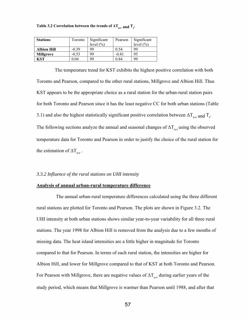
57

Table 3.2 Correlation between the trends of ΔTu-r and Tr.

Stations Toronto Significant

level (%) Pearson Significant

level (%) Albion Hill -0.39 99 0.54 99 Millgrove -0.53 99 -0.81 95 KST 0.04 99 0.84 99 The temperature trend for KST exhibits the highest positive correlation with both

Toronto and Pearson, compared to the other rural stations, Millgrove and Albion Hill. Thus

KST appears to be the appropriate choice as a rural station for the urban-rural station pairs

for both Toronto and Pearson since it has the least negative CC for both urban stations (Table

3.1) and also the highest statistically significant positive correlation between ΔTu-r and Tr.

The following sections analyze the annual and seasonal changes of ΔTu-r using the observed

temperature data for Toronto and Pearson in order to justify the choice of the rural station for

the estimation of ΔTu-r .

3.3.2 Influence of the rural stations on UHI intensity

Analysis of annual urban-rural temperature difference

The annual urban-rural temperature differences calculated using the three different

rural stations are plotted for Toronto and Pearson. The plots are shown in Figure 3.2. The

UHI intensity at both urban stations shows similar year-to-year variability for all three rural

stations. The year 1998 for Albion Hill is removed from the analysis due to a few months of

missing data. The heat island intensities are a little higher in magnitude for Toronto

compared to that for Pearson. In terms of each rural station, the intensities are higher for

Albion Hill, and lower for Millgrove compared to that of KST at both Toronto and Pearson.

For Pearson with Millgrove, there are negative values of ΔTu-r during earlier years of the

study period, which means that Millgrove is warmer than Pearson until 1988, and after that

58

due to the impact of urbanization Pearson became warmer than Millgrove which is observed

from the positive ΔTu-r. If the temperature differences at Toronto and Pearson were caused

only by the urban effect, then the year-to-year variation pattern would be expected to remain

the same, no matter which rural station provided the data to compute ΔTu-r. However, this is

not what is observed in Figure 3.2.

Toronto

0

1

2

3

4

5

19701973

19761979

19821985

19881991

19941997

2000

Years

U-R

tem

pera

ture

diff

eren

ce ºC

tor-albtor-milltor-king

Pearson

-1

0

1

2

3

4

19701973

19761979

19821985

19881991

19941997

2000

Years

U-R

tem

pera

ture

diff

eren

ce ºC

pear-albpear-millpear-king

Figure 3.2 Year-to-year variation of UHI intensity at Toronto and Pearson with three rural stations for the period of 1970-2000

59

In order to do a more detail examination of the temperature time series of ΔTu-r, the Mann-

Kendall trend test, which is more robust in situations with missing data or when the

assumption of normal distribution cannot be assumed, is applied to observe the pattern of the

long term trends of UHI at Toronto and Pearson. The magnitude of the trends is calculated

using the TSA approach, and the results are presented in Tables 3.3 and 3.4 as °C/decade.

According to the analysis, positive trends are found in all cases at Toronto except for

minimum and mean ΔTu-r for Albion Hill and for maximum ΔTu-r for Millgrove. For Pearson,

positive trends are observed in all cases except for maximum ΔTu-r when Millgrove is

considered as a rural station. The trends for minimum ΔTu-r were statistically significant at

99% level for all three rural stations for Pearson. However, for Toronto, the minimum ΔTu-r

trends were statistically significant at 99% level only when Millgrove is taken as a rural

station. In the case of Toronto with Albion Hill, a negative trend for Tu-r for annual mean

temperature is observed. When Millgrove is used, the trend for annual mean ∆Tu-r is the

highest compared to the other stations. With KST, the increasing annual trend for ∆Tu-r is

consistent with the gradual increase in the magnitude of ∆Tu-r with the ongoing pace of

urbanization over the years observed in Figure 3.2, particularly for Pearson. Although the

choice of KST as the rural station shows urban warming at both Toronto and Pearson, more

analysis is required to make a clear decision on the choice of the rural station. However, it is

evident at this point of the analysis that the choice of a rural station has a significant impact

on the quantification of UHI intensity at both Toronto and Pearson.

60

Table 3.3 Estimated trends of annual UHI intensity for Toronto using Mann-Kendall test

for the period of 1970-2000, (°C/decade)

Table 3.4 Estimated trends of annual UHI intensity for Pearson using Mann-Kendall test

for the period of 1970-2000, (°C/decade) Stations

∆Tu-r_max

∆Tu-r_min

∆Tu-r_mean

Pear-Alb **0.007 **0.008 **0.008

Pear-Mill -0.005 **0.03 **0.009 Pear-King **0.005 **0.02 **0.01

* Significant at 95%, **Significant at 99% An important observation that can be made from the above analysis is that the

“urban heat islands” that exist at Toronto and at Pearson are different in magnitude (Figure

3.2). While it is apparent from Figure 3.2 that the changes in ∆Tu-r are higher for Toronto

than that for Pearson, however, the trend analysis suggests that the magnitude of the trends

are higher for Pearson compared to that of Toronto in all cases of ∆Tu-r. The trends for UHI

intensities are 4% and 16% higher for the minimum and maximum ∆Tu-r, respectively, at

Pearson compared to that at Toronto when using KST as the rural station. In addition, the

annual mean trends of ∆Tu-r are statistically significant for Pearson but not for Toronto in

case of all the rural stations. This observation could be attributed to the findings in chapter 2,

where it was suggested that at Toronto downtown the UHI has reached a saturation point in

terms of urban warming, and thus the trends for annual mean ∆Tu-r doesn’t show any

significant changes.

Although other meteorological factors such as wind, rain, clouds, near-surface

temperature lapse-rate may have impacts on the urban heat island, the difference in the trend

results between Table 3.3 and 3.4 could be attributed to the relationship among UHI

Stations ∆Tu-r_max ∆Tu-r_min ∆Tu-r_mean Tor-Alb 0 -0.005 -0.001 Tor-Mill **-0.009 **0.01 0.006 Tor-King 0.0008 0.0008 0.0004

61

intensity, near-surface phenomenon and the localized topographic effect on the temperature.

On a hot day, the city warms faster than the land and air rises over the city. This creates the

on-shore lake breeze, which is the case for Toronto. Under such conditions a greater

mechanical mixing would cause an elevated inversion destroying lower level inversion with

an increasing frequency of the unstable conditions during the day hours over the city (Hirt

and Shaw, 1973; Yap, 1975; Godowitch et al., 1985). This is expected to reduce the effect of

urban heat island at Toronto. Without the lake effect the inversion would persist longer at the

city and would not help to diminish the urban heat island effect, which is likely the case for

Pearson. During the cold seasons, if there is a lake in the vicinity two situations can result

depending on the ice cover over the lake. If the lake is covered with ice, which occurs with

Lake Ontario approximately every ten years, then the air over land is warmer than the air

over the lake. Under such condition, the warm air from land flows over the lake and the air

chills, which causes an inversion. If the lake is not covered with ice, which is a frequent

condition with Lake Ontario, then the temperature gradient between land and water should be

very small. However, in the presence of the UHI effect, the air over land is warmer than the

lake, and the warm air from land flows over the lake and the air chills, which causes an

inversion. This inversion promotes stability within the vertical layers of the troposphere

within the air over the lake and a weak lapse rate period is expected in the city. In general,

during cooler periods of the year with stronger vertical stability and increased frequency of

stable conditions there should be an increase in urban heat island effect. Thus during colder

months of the year, particularly in winter, UHI effect has a positive feedback to create

vertical stability by strong inversion and vice versa.

Toronto experiences a direct lake effect, whereas, Pearson experiences no direct

lake effect. Therefore, due to the presence of the lake the heat island effect will have a

62

mitigating effect on temperature trends for Toronto which is absent for Pearson. It is thus

suggested that Toronto will experience strong heat island effect on minimum temperature,

but a mitigating effect from the lake on the maximum temperature, particularly in summer as

explained above and also observed by Gough and Rozanov (2001). In general, the effect of

any urban warming is expected to be more pronounced on minimum temperature compared

to that on the maximum temperature (Lee, 1975; Godowitch, et al., 1985; Johnson et al.,

1991; Kalnay and Cai, 2003). In addition to the lake effect another reason for increasing

trends of ∆Tu-r at Pearson compared to Toronto is that during 1970-2000 massive

urbanization has been taken place near the airport areas, while the city core might have

reached at the saturation point in terms of urban warming (See Chapter 2). The question that

arises at this point is: is the UHI intensity with or without the lake effect the same with three

different rural stations? Essentially the UHI intensity is considerably different in the case of

each rural station at both Toronto and Pearson, which can be related to the distinctive

physical and climatic nature of individual rural stations, an issue which is explored further in

the following sections.

3.3.3 Analysis of seasonal variation of urban-rural temperature difference

Seasonal distribution of UHI intensity

The variation of monthly mean temperature differences between the two urban

stations and the three rural stations, Albion Hill, Millgrove and KST are shown in Figure 3.3.

The urban heat island intensity at Toronto seems to be higher during December, January and

February, however, with differing strengths for the three rural stations. The heat island

intensity at Pearson shows a similar pattern for Albion Hill and Millgrove but a different one

for KST. To study the features of the seasonal variation of urban-rural temperature

63

difference, winter is classified as December, January and February, spring is classified as

March, April and May, summer is classified as June, July and August and finally autumn is

classified as September, October and November. The seasonal changes in urban-rural

temperature difference computed using the three rural stations for the period of 1970-2000

are shown in Figure 3.4 for Toronto and Pearson.

Toronto

0.00

1.00

2.00

3.00

4.00

Jan Feb Mar Apr May Jun Jul Aug Sep Oct Nov DecMon

thly

mea

n u

rban

-rura

l tem

pera

ture

di

ffere

nce,

°C

Tor-Alb

Tor-Mill

Tor-King

Pearson

-0.50

0.00

0.50

1.00

1.50

2.00

Jan Feb Mar Apr May Jun Jul Aug Sep Oct Nov DecMon

thly

mea

n u

rban

-rur

al

tem

pera

ture

diff

eren

ce, °

C

Pear-Alb

Pear-Mill

Pear-King

Figure 3.3 Monthly mean changes of urban-rural temperature difference at Toronto and Pearson with three different rural stations for the period of 1970-2000

64

In order to analyze the seasonal variation of ∆Tu-r, two types of patterns are

identified to characterize the changes in UHI intensity; UHI intensity that is dominating in

the cooler part of the year, or winter dominating, and UHI intensity that is dominating in the

warmer part of the year, or summer dominating. In the case of Toronto for all three rural

stations, the ∆Tu-r is higher in winter compared to summer. With the rural stations Albion

Hill and Millgrove, Toronto exhibits similar patterns in seasonal variation of the UHI

intensity, while with KST the variation is a little different. For Pearson, the UHI intensity is

higher in summer with Albion Hill and Millgrove, but higher in winter for KST. The

magnitude of the seasonal UHI intensity is the lowest for Millgrove for all seasons. Albion

Hill has the highest values of UHI intensities for all seasons except for winter. Finally, with

KST the UHI intensity is found to be the highest in winter compared to the other two rural

stations for both Toronto and Pearson. The factors that are considered to explain these

observations are as follows: i) the location of the rural station in relation to the urban station,

ii) the influence of the geography and environment surrounding the rural station on the

seasonal temperature time series (Tu-r), and iii) the distance of both the urban and rural

stations from a water body.

Figure 3.1 (Section 3.2) shows that Albion Hill is situated to the northwest of

Toronto and Pearson, and is surrounded by the Oak Ridge Moraine conservation area. There

are a few farms, golf courses and campgrounds nearby, however, for the past few years

concrete has been built up in the surrounding areas. In terms of water body, there are a

number of creeks situated near the meteorological station. The rural station, KST is situated

to the north of Toronto and Pearson, and 70% of its land conserves a typical countryside

setting with an assortment of farmlands. It should be noted that this station is farthest from

65

both the urban stations compared to the other two rural stations. The station, Millgrove is

situated to the southwest of Toronto and Pearson and is 0.6°C warmer than KST and 1°C

warmer than Albion Hill. It also has a number of agricultural and farm lands nearby. This

station is also close to Lake Ontario compared to the other two rural stations, which are

located further inland. In terms of the observed seasonal temperatures, Millgrove experienced

the highest average seasonal temperatures (Tr_seas) temperatures among the three rural

stations during 1970-2000. Consequently, the seasonal ∆Tu-r estimated with Millgrove as a

rural station shows the lowest magnitude of UHI intensities (Figure 3.4).

In Chapter 2 it was suggested that urban heat island is more pronounced on the

minimum temperature than on the maximum temperature at Toronto. In the current study the

former is observed for Albion Hill and KST and the latter is observed for Millgrove.

Therefore, the UHI intensity can be characterized as winter dominating at Toronto using both

Albion Hill and KST as the rural station, while it shows a balance between winter and

summer when Millgrove is used to compute ∆Tu-r. For Pearson, UHI intensity is clearly

summer dominating when Millgrove is selected as a rural station and winter dominating

when KST is used to compute ∆Tu-r. There is a balance between winter and summer when

Albion Hill is used as a rural station for Pearson. Inland areas are generally hotter in summer

and colder in winter than the areas near a water body. Therefore, the observed UHI at

Toronto with Millgrove (both are influenced by the lake) has a physical reason to show

balance between winter and summer. However, this is not the case for Pearson for which the

UHI intensity shows summer dominating characteristic with Millgrove as the rural station. A

recent study of Tokyo’s UHI suggested that it is necessary to select a rural station that has the

same distance from a water body as the urban station to calculate the heat island magnitude

66

accurately (Sakakibara and Owa, 2005). Thus for Toronto, Millgrove could be a better station

to compute ∆Tu-r since both experience the lake effect.

Another important observation is that the magnitude of ∆Tu-r is higher when using

Albion Hill than when using KST as the rural station for Toronto, although the latter retains

70% of its land with rural characteristics. This can be attributed from the effect of land use as

agricultural development on the maximum and minimum temperatures of KST. The use of

land for agriculture has an impact on the decrease in maximum temperature in the

surrounding areas due to increasing evaporation throughout the day. Also, irrigation would

increase the heat capacity of the soil and thus would increase the minimum temperature from

reduction of evaporation at night. Therefore, both urbanization and agriculture have similar

impacts on the temperature change, which is to increase the minimum temperature (Kalnay

and Cai, 2003).

Toronto

0.0

0.5

1.0

1.5

2.0

2.5

3.0

3.5

4.0

Winter Spring Summer Autumn

∆Tu-

r, °C

Tor-Alb

Tor-King

Tor-Mill

Pearson

-0.5

0.0

0.5

1.0

1.5

2.0

Winter Spring Summer Autumn

∆Tu-

r, °C

Pear-Alb

Pear-King

Pear-Mill

Figure 3.4 Seasonal changes in ∆Tu-r at Toronto and at Pearson for three different rural stations for the period of 1970-2000

67

The fact that with KST, the estimated UHI intensities for both Toronto and Pearson are much

less in magnitude than Albion Hill is because of the two different physical phenomena but

with similar impacts on the temperature that cancel out some of the UHI effects. To

summarize, at both Toronto and Pearson the UHI intensities can be characterized as winter

dominating irrespective of the choice of different rural stations to compute the ∆Tu-r. The

only exception is when Millgrove is used as a rural station for Pearson. These observations

are clarified further with the analysis of UHI in different seasons and the results from the

trend analysis of the seasonal time series for ∆Tu-r.

Frequency of the seasonal distribution of UHI intensity

Figure 3.5 shows an analysis of the frequency of seasonal UHI intensities at

Toronto and Pearson. For Toronto using Albion Hill as the rural station, a higher frequency

of UHI intensities is observed in summer and autumn than in winter and spring. A similar

observation is also evident for Pearson. Using Millgrove, the higher frequencies are observed

in autumn compared to the other seasons at both Toronto and Pearson. With KST as a rural

station the higher frequencies of UHI are observed in winter than in the other seasons at both

Toronto and Pearson. The frequency of UHI intensities with KST as the rural station is

dominant in cooler seasons than in warmer seasons with a slightly higher magnitude at

Toronto than at Pearson.

Toronto is situated at temperate latitude, and in general, in temperate latitude cities,

the seasonal variation of UHI is evident with the greatest frequency of occurrence being

registered in the warmer part of the year (Oke, 1979). However, due to the presence of the

68

lake this observation is reversed for Toronto, that is, the greatest frequency of UHI is

observed during the colder part of the year.

Toronto-Albion Hill

0%

10%

20%

30%

40%

50%

60%

70%

80%

90%

100%

0-2 2-3 3-4 4-5 5-7 >7

Temperature difference,U-R (°C)

UH

I int

ensi

ties

(%)

AutumnSummerSpringWinter

Pearson-Albion Hill

0%

10%

20%

30%

40%

50%

60%

70%

80%

90%

100%

0-2 2-3 3-4 4-5 5-7 >7

Temperature difference, U-R (°C)

UH

I int

ensi

ties

(%)

AutumnSummerSpringWinter

Toronto-Millgrove

0%

10%

20%

30%

40%

50%

60%

70%

80%

90%

100%

0-2 2-3 3-4 4-5 5-7 >7

Temperature difference, U-R (°C)

UH

I int

ensi

ties

(%)

AutumnSummerSpringWinter

Pearson-Millgrove

0%

10%

20%30%

40%

50%

60%

70%80%

90%

100%

0-2 2-3 3-4 4-5 5-7 >7

Temperature difference, U-R(°C)

UH

I int

ensi

ties

(%)

AutumnSummerSpringWinter

Toronto-KST

0%

10%

20%

30%

40%

50%

60%

70%

80%

90%

100%

0-2 2-3 3-4 4-5 5-7 >7

Temperature difference, U-R(°C)

UH

I int

ensi

ties

(%)

AutumnSummerSpringWinter

Pearson-KST

0%

10%

20%

30%

40%

50%

60%

70%

80%

90%

100%

0-2 2-3 3-4 4-5 5-7 >7

Temperature difference, U-R(°C)

UH

I int

ensi

ties

(%)

AutumnSummerSpringWinter

Figure 3.5 Frequency of intensity of UHI at Toronto and at Pearson for three different rural stations for the period of 1970-2000

69

Criteria to choose a rural station

It was assumed from the correlation analysis (Section 3.3.1) that KST is an ideal

choice for Toronto as a rural station to compute ∆Tu-r. It is critical to understand, however,

that whether ∆Tu-r computed with Albion Hill or Millgrove or that computed with KST is

more consistent with the climatic and geographical features of Toronto and Pearson. A

detailed look at the results from the trend analysis of seasonal ∆Tu-r (Tables 3.5 and 3.6)

suggest that statistically significant increasing trend of UHI intensity exists at Toronto mainly

for winter with Millgrove and KST, while for Albion Hill no statistically significant trend for

seasonal ∆Tu-r is detected . Therefore, considering the annual and seasonal climatic

characteristics of UHI intensities discussed above, for Toronto, Albion Hill can be considered

as a less suitable choice of a rural station to quantify the UHI intensity. For Pearson,

statistically significant increasing trends are observed for almost all seasons with all three

rural stations making it difficult to identify an appropriate rural station to compute ∆Tu-r. It

was established earlier that both Toronto and Pearson experience UHI intensities that are

winter dominating. The choice of Millgrove as a rural station, which shows winter

dominating ∆Tu-r for Toronto, seems to be reasonable considering the geographic features

that is, the effect of the lake at both urban and rural stations. However, in terms of

magnitude and frequency distribution, the UHI intensity computed with KST shows all the

seasonal characteristics for Toronto including increased frequency in winter compared to

summer. For Pearson, with winter dominating ∆Tu-r, KST or Albion Hill could be a better

choice from a climatic standpoint than Millgrove for which urban heat island effect is more

pronounced in summer (Figures 3.3 and 3.4).

70

Table 3.5 Estimated trends for seasonal ∆Tu-r for Toronto using Mann-Kendall test (°C/decade)

Stations

∆Tu-r_Winter

∆Tu-r_Spring

∆Tu-r_Summer

∆Tu-r_Autumn

Tor-Alb -0.009 -0.008 0.03 0.0009 Tor-Mill **0.01 0.008 -0.003 *0.01 Tor-King *0.009 -0.006 *0.02 0

Table 3.6 Mann-Kendall test results from trend analysis of seasonal ∆Tu-r for Pearson (°C/decade)

Stations

∆Tu-r_Winter

∆Tu-r_Spring

∆Tu-r_Summer

∆Tu-r_Autumn

Pear-Alb **0.01 *0.015 **0.07 **0.03 Pear-Mill **0.04 **0.03 **0.03 **0.04 Pear-King *0.01 **0.02 **0.06 **0.03 * Significant at 95%, **Significant at 99% According to the IPCC the estimated uncertainty due to the impact of UHI effect on

the annual mean temperature trend is reported between 0.006 to 0.007 °C/decades since 1990

to present for the Northern Hemisphere (Trenberth et al., 2007). This magnitude is close to

the trend of the ∆Tu-r estimated with Millgrove as a rural station for Toronto

(0.006°C/decade) for the period of 1971-2000 (Table 3.3). With KST as a rural station the

annual mean trend for UHI intensity (0.0004°C/decade) may be underestimated reflecting the

bias of climatic characteristics of an inland site as a rural station (Table 3.3). Although, the

results from the trend analysis of ∆Tu-r with KST as a rural station suggest an

underestimation of UHI intensities for Toronto, the station cannot be ruled out completely

because the characteristics of annual and seasonal UHI intensity using KST as a rural station

are consistent with the observed local climate of Toronto. The uncertainty reported by IPCC

due to UHI effect is also comparable to the trend of the annual mean ∆Tu-r at Pearson

(0.008°C/decade) with Albion Hill as a rural station (Table 3.4). However, Albion Hill is a

less suitable choice as a rural station from a climatic standpoint due to the summer

dominating characteristic which may overestimate the urban heat island effect. With KST as

a rural station for Pearson, the annual trend of ∆Tu-r show similar seasonal characteristics as

71

Toronto with a little higher magnitude. The estimated annual warming due to the effect of

urbanization at Toronto after the elimination of the background climate change, therefore,

ranges from 0.004 to 0.006°C/ decade depending on the choice of an inland rural station or a

rural station close to the lake similar to Toronto. For Pearson the range of UHI intensity is

between 0.008 to 0.01°C/decade, and the magnitude increases if the rural station is further

inland from Pearson.

3.3.4 Analysis of the Diurnal variation of UHI intensity in winter and summer

In order to characterize the diurnal variation of UHI intensity at Toronto and

Pearson in winter and summer, the temperature time series for February and July, 2006, are

considered, respectively. The reason to choose 2006 is that this is the latest year for which

hourly data is available for the city of Toronto. The choice of the months is a result of the

observation that at Toronto in winter the lowest average temperature is experienced in

February and in summer the highest average temperature is experienced in July. The rural

stations that are considered so far in this study do not have hourly temperature data,

therefore, another rural station, Beatrice, which is located outside the Greater Toronto Area

(GTA), further north of King Smoke Tree, is used to compute the hourly ∆Tu-r for Toronto

and Pearson. Beatrice and KST have comparable temperature time series with a difference in

mean of 0.6°C for 2006 (shown in Appendix 1) and show a similar pattern of temperature

change for the year 2006.

In order to select the days for the analysis of the diurnal variation of UHI at Toronto

and Pearson, initially the change of the amplitude of UHI in July and February in relation to

the wind speed was examined (Figure 3.6). The reason for this investigation is that, in

72

general, urban heat island effect tends to get weaker with higher wind speed in the city,

whereas it is more evident under calm and clear conditions (Munn et al., 1969). Therefore,

the examination of Figure 3.6 provides a clear idea about the dependency of the formation of

UHI under various synoptic conditions. During winter, in February 2006, there are 22 and 19

days with UHI greater than 5°C at Toronto and at Pearson, respectively. According to the

Spatial Synoptic Classification (SSC) of day-to-day weather (Sheridan, 2002), the DP (dry

polar) weather category was prominent throughout the month of February, which is

favourable to the formation of UHI (See Appendix 2 for detail of SSC). On the other hand,

the dominant SSC weather category for the month of July was MT (moist tropical), which

creates cyclonic conditions due to the passage of the MT air mass (Sheridan, S.,

http://sheridan.geog.kent.edu/ssc2.html). In July the number of days with UHI greater than 5°C at

Toronto and at Pearson are only 2 and 4 days, respectively. This observation is consistent

with the fact that UHI is more pronounced in winter than in summer at Toronto and Pearson

(Section 3.3.2).

73

Toronto

0

1

2

3

4

5

6

7

1 3 5 7 9 11 13 15 17 19 21 23 25 27 29 31

Days of July

ΔTu

-r, °C

0

1

2

3

4

5

6

7

win

d sp

eed

(m/s

)

Pearson

0

1

2

3

4

5

6

7

1 3 5 7 9 11 13 15 17 19 21 23 25 27 29 31

Days of July

ΔTu

-r,°C

0

1

2

3

4

5

6

7

8

win

d sp

eed

(m/s

)

Toronto

0

2

4

6

8

10

12

14

1 3 5 7 9 11 13 15 17 19 21 23 25 27

Days of February

ΔTu

-r, °C

0

2

4

6

8

10

12

14

win

d sp

eed(

m/s

)

Pearson

0

2

4

6

8

10

12

14

1 3 5 7 9 11 13 15 17 19 21 23 25 27

Days of February

ΔTu

-r, °C

0

2

4

6

8

10

12

14

win

d sp

eed(

m/s

)

ΔTu-r wind speed Figure 3.6 Change in the amplitude of UHI intensity at Toronto and Pearson in relation to wind speed for July and February, 2006

The strongest UHI was experienced on February 9-10, 2006 at both Toronto and Pearson.

Therefore, these days were considered for the analysis of the diurnal variation of UHI in

winter. In summer, on July 2-3, 2006, the UHI was the strongest and these days were

considered for the investigation of the diurnal variation of UHI. Figure 3.7 compares the

variation of UHI on 2-3 February and on 9-10 July.

74

July 02-03, 2006

0

2

4

6

8

10

12

9:0010

:0011

:0012

:0013

:0014

:0015

:0016

:0017

:0018

:0019

:0020

:0021

:0022

:0023

:00 0:00

1:00

2:00

3:00

4:00

5:00

6:00

7:00

8:00

Hours

∆Tu-

r (ºC

)

February 09-10, 2006

0

4

8

12

16

20

24

9:0010

:0011

:0012

:0013

:0014

:0015

:0016

:0017

:0018

:0019

:0020

:0021

:0022

:0023

:00 0:00

1:00

2:00

3:00

4:00

5:00

6:00

7:00

8:00

Hours

∆Tu-

r (ºC

)

∆Tu-r_tor ∆Tu-r_pear Figure 3.7 Comparison of the diurnal variation of UHI intensity in July and February between Toronto and Pearson.

On February 09-10, 2006, there were anti-cyclonic conditions dominating over Toronto

resulting in clear and dry conditions, which is favourable for the formation of urban heat

island. On Feb 09, there was a weak positive UHI all through the day, with wind speed

ranging from 5-9 m/s, which started to develop significantly right after the sunset, and by

midnight the UHI was at its peak in magnitude with wind speed of only 2 m/s. Around 5:00

am on February 10 another anti-cyclone passed over Toronto and the UHI reached its peak

75

once again at 7:00 in the morning with a wind speed of 4 m/s, after which the heat island

effect started to diminish. Since SSC considers the large scale air mass that passes over

Toronto, therefore, under similar synoptic condition, with wind speed ranging from 7-10 m/s

during the day, at Pearson Airport the development of UHI on February 09-10 follows a

similar pattern as Toronto except with a little higher magnitude than Toronto which evens out

at 6:00 am (wind speed 1 m/sec) in the morning on February 10. The direction of the wind is

predominantly from SW on Feb 09-10 at both Toronto and Pearson. Figure 3.8 compares the

changes of UHI in terms of their magnitude for Toronto and Pearson.

On July 02-03, there were anti-cyclonic conditions dominating on both days with

moist tropical (MT) air at Toronto causing warm and humid conditions. There was a well

developed UHI on 02 July between 9:00 and 13:00 with a wind speed of 6 to 10 m/s, which

started to weaken between 14:00 to19:00 and then reached its peak at 22:00 with a wind

speed of 2 m/s. The UHI started to fade again after sunset around 23:00 due to the effect of

the lake breeze at Toronto with a wind speed of 13 m/s coming from the south, whereas at

Pearson the UHI was still dominant until 01:00 without the effect of the lake breeze. The

increase of UHI magnitude after sun set shows the fact that rural areas cool down faster since

the heat capacity of rural areas is much lower than that of urban areas. The changes in the

magnitude of UHI in July is presented in Figure 3.8, which clearly shows the mitigating

effect of the lake on UHI intensity at Toronto compared to that at Pearson with little or no

lake effect. In general, both Toronto and Pearson experiences UHI of relatively high

magnitude in winter compared to that of summer, particularly at night, with or without the

lake effect. This is evident from Figure 3.8 where the bars, which are proportional to the

magnitude of UHI, are higher for February than that for July.

76

(a) July (02-03)

77

(b) February (09-10)

Figure 3.8 Diurnal changes in UHI intensity at Toronto and Pearson on (a) July (02-03) and (b) February (09-10), 2006;(the bars are proportional to the magnitude of UHI intensity)

78

3.4 Summary and Conclusions In this chapter the impact of the choice of a rural station to estimate the urban heat

island intensity was examined for Toronto. The urban heat island effect at Toronto was

analyzed using three different rural stations, Albion Hill, Millgrove and King Smoke Tree

(KST), with different topographic and climatic characteristics. To account for the lake effect

another urban station Toronto Pearson without direct lake effect was also used to estimate the

UHI intensities. At the beginning of the analysis KST was predicted to be a suitable choice

for Toronto and also for Pearson from the correlation analysis. The UHI intensity was

estimated using each rural station and two types of intensities were observed: winter

dominating and summer dominating depending on the choice of the rural station.

Previous studies suggested that at Toronto UHI effect is less pronounced in

summer due to the presence of the lake (Gough and Rozanov, 2001). The analysis of the

annual and seasonal time series of the ∆Tu-r confirms the winter dominating character of

UHI intensities for Toronto, and also for Pearson. The analysis of the frequency distribution

of seasonal UHI suggested that the frequencies are higher in winter only for KST, while for

Albion Hill the frequency is higher in summer and autumn, and finally, for Millgrove the

frequency distribution is dominant in spring and autumn. It was suggested from the trend

analysis of ∆Tu-r that if a rural station such as Millgrove, with the similar geographic and

climatic features as Toronto (both are situated near Lake Ontario) is used to compute the

annual mean ∆Tu-r then the magnitude of UHI intensity (0.006°C/decade) is in good

agreement with that suggested by the IPCC for the Northern Hemisphere (0.006°C/decade).

If an inland station such as KST is considered then the magnitude of UHI intensity

(0.0004°C/decade) is lower than that of Millgrove. This leads to a potential underestimation

of the UHI intensity. Therefore, the initial prediction that KST is a suitable choice as a rural

79

station is not in agreement with the trend analysis. However, it is also not possible to rule out

KST as a rural station completely because the analyses of annual and seasonal distribution of

UHI intensities using this station show climatic characteristics that are consistent with the

observed climate of Toronto and Pearson. It is thus suggested that the current practice that

exists in the urban climate literature for the selection of a unique pair of urban-rural to

compute UHI intensity is arbitrary. The current study raised the question as ‘what is a unique

urban-rural pair to estimate the UHI intensity’. The study reveals that the choice of a pair to

estimate ∆Tu-r is dependent on the topographic and climatic characteristics of the urban and

rural stations, and also more importantly on the objective of a particular study in the context

of UHI effect. The critical first step is to identify a proper rural and urban station to compute

∆Tu-r considering more than one criterion such as physical characteristics, population

distribution, satellite night-light data if available etc, and then to use the correlation method

to identify an appropriate pair. Therefore, it can be suggested that in future the urban

climatologists should take initiatives to set a standard or rules in order to choose an

appropriate urban-rural pair that can be used universally for the UHI study.

The analysis of the diurnal variation of UHI in winter and summer at Toronto and

Pearson suggested that the magnitude is much higher in winter compared to summer, with a

weak urban heat island developing during daytime compared to a well developed one at

night. The magnitude of the diurnal UHI intensity is comparatively lower at Toronto in

summer than that at Pearson due to the presence of the lake. The UHI effect starts to

dominate immediately after sunset and persists longer at night in winter under calm and clear

condition than in summer. The favourable synoptic conditions (SSC category, DP) at Toronto

in winter months leads to the formation of urban heat island with much higher frequency

during winter compared to summer.

80

Chapter 4: Analysis of Trends for Extremes Indices of Daily Observed Temperature in the Greater Toronto Area (GTA)

4.1. Introduction

The research on extreme weather and climate change due to anthropogenic activities

has become increasingly important because the greatest impact of climate change may result

from the changes in the extremes, rather than in the mean. Successive reports (Folland et. al.,

2001; Trenberth et al., 2007) of the Intergovernmental Panel on Climate Change (IPCC) have

identified that the detection of trends and variability in extreme temperatures are critical

factors to understand the nature of past and future climate change. These reports indicate that

extreme events usually have the greatest and most immediate societal impact, which is often

associated with high economic and human costs. Therefore, monitoring, detecting and

attributing changes in climate extremes can contribute our understanding of risk due to

changes in climate.

Analyses of the observed daily temperature in many parts of the globe have already

shown important changes in the extremes (Vincent and Mekis, 2006; Aguilar et al., 2005;

Vincent et al., 2005; Frich et al., 2002; Peterson et al., 2002; Zhang et al., 2000; Bonsal et al.,

2001; Easterling et al., 2000). These studies considered a period ranging from 1900 to 2003

and showed that there is a general increase in extreme warm nights and hot days but found

fewer extreme cold days and cold nights. Investigation of the trends in temperature indices

over Europe suggested that the annual number of warm extremes (for the period of 1961-

1990) for daily temperature increased twice as rapidly during the last 25 years than the

81

expected corresponding decrease in the number of cold extremes (Klein Tank and Können,

2003) for the same period. Vincent et al. (2005) found that in southern South America there

is significant increasing (decreasing) trends of warm (cold) nights, however, no consistent

changes in the indices based on maximum temperature was detected. In China, decreasing

warm and cold extremes are found during the late 19th century and increasing warm

extremes only since 1961 (Yan et al., 2002). In the United States, slight downward trend of

the frequency of days with maximum temperature above the 90th percentile was observed for

the period of 1910-98 (Easterling et al., 2000). A study of North America suggested a strong

warming of the lowest daily minimum temperatures over the western and central North

America during 1948-2000 (Robeson, 2004). A near-global study on the trends in extreme

temperature reported coherent spatial pattern in extreme changes including an increase in

warm summer nights, decrease in the number of frost days and intra-annual extreme

temperature range (Frich et al., 2002). Several studies exist on the analyses of extremes in

Canada. Bonsal et al. (2001) detected significant increasing trends for the lower and higher

percentiles of the daily minimum and maximum temperature distribution for Southern

Canada for the period of 1900-98. A more recent study by Vincent and Mekis (2006) found

fewer extreme cold nights and cool days but more extreme warm nights and hot days for

Canada during 1900-2003.

Many studies on temperature extremes have also focused on economically important

indices such as heating degree days (HDD) and cooling degree days (CDD), which are

related to the changes in daily observed temperature. In general, climate change is

accompanied by enhanced amount of energy consumption, which in turn is responsible for

the increase of atmospheric greenhouse gases. A study on the trends in seasonal HDD and

CDD for Turkey for 74 climatological sites suggested that topography, macro and

82

microclimate features have considerable impacts on the observed trends in HDD and CDD

(Kadioğlu, 2001). Analysis of HDD and CDD trends for Southern Québec suggested that

cooling degree days have increased while heating degree days have decreased over the period

of 1960-2005 (Yagouti et al., 2007). Bonsal et al. (2001) compared the changes in HDD and

CDD over Canada for two different periods, and suggested that there is significant increase

in CDD trends and decrease in HDD trends during 1950 to 1998 compared to 1900 to 1998.

A few studies attempted to establish a link between the trends in HDD/CDD and urban heat

island effect. For example, in Minnesota, USA, the HDD totals for the year 1989 is found to

vary by 545 heating degree days between an urban and a rural site. The study also reported

that maximum CDD total occurs over the city center ((Todhunter, 1996). A study on the

urbanization impacts in Phoenix, Arizona found that the number of cooling degree days have

increased from 1560 to 2130 due to urban warming for the period of 1948-2000. The number

of heating degree days has also declined from 695 to 364 for the same period (Baker et al.,

2002).

In most of the studies discussed above linear trend analysis is used on the available

annual and seasonal temperature data. However, for a better holistic understanding of both

past and potential future changes to climate extremes, analyses at the daily time scale are

essential. The indices that are analyzed in various studies of extremes were chosen

considering several factors including the availability of the data, indices appropriate for the

study area of interest, and in some cases solely on the objective of the study. This chapter

examines the trends of daily temperature extremes in the Greater Toronto Area (GTA),

Ontario, Canada, for the period of 1971-2000. Using the best available daily temperature

data, spatial and temporal aspects of the extreme indices are investigated. The data and

methodologies are discussed in Section 4.2 and the analysis of the trends of extreme indices

83

is presented in Section 4.3. The analysis of the economically sensitive indices based on daily

mean temperature is also presented in Section 4.3. A summary and conclusion of the findings

follow in Section 4.4.

4.2. Data and methodologies

4.2.1 Data

Temperature data used in this study consist of daily minimum and maximum values for

nine stations in the GTA (Figure 4.1 and Table 4.1). The period of record used in this study is

from 1971 to 2000 for all stations except for King Smoke Tree, for which data for 1974-2000

only is available. The time series of temperatures are tested for homogeneity using the Mann-

Whitney (MW) homogeneity test. The MW test is a non-parametric rank-based test for

identifying difference between two samples with respect to their median or means. The two

samples are combined and all sample observations are ranked from smallest to largest. If the

two samples have the same distribution then the sum of the ranks of the first sample and

those in the second sample should be close to the same value (Yue and Wang, 2002). The

advantage of the MW test compared to other parametric tests (e. g. Bartlett test, t test) is that

the test can be applied to data without the assumptions of normal distribution, and to large

data samples (von Storch and Zwiers, 1999). Therefore, it is more robust for temperature

measurements, which are affected by changes in the location of the weather station, changes

in observing practices and changes in instrumentation. Since any erroneous outlier can have

a serious impact on the estimation of the trends in extremes, data quality assessment is

essential before the calculation of the indices. All the temperature time series were, therefore,

examined for suspicious daily values such as maximum temperature less than minimum

84

temperature and daily values outside of four standard deviations from the mean for a

particular time of the year. The unusual values were compared with nearby stations. The data

was also checked manually to assess if the flawed values were a part of a cold or warm spell.

Finally, all the erroneous values were listed as missing before the indices were calculated.

Table 4.1 Meteorological stations in the Greater Toronto Area (GTA)

Station name Station location Elevation(m) Type Longitude Latitude Toronto downtown -79. 40 43.67 112 Urban Toronto Pearson -79’ 60” 43. 67 173 Urban Toronto Island -79.40 43.63 76 Urban Richmond Hill -79. 45 43.88 240 Suburban Woodbridge -79. 60 43.78 164 Suburban Oshawa -78.87 43.90 113 Suburban Albion Hill -79. 83 43.92 281 Rural Millgrove -79.97 44.32 352 Rural King Smoke Tree -79.52 44.02 255 Rural

Figure 4.1 Map showing the stations used for extreme temperature analysis in the GTA

85

4.2.2 Selected indices for temperature

The ideal extreme indices of climate parameters have some desirable characteristics.

The selected indices should be associated with local impacts of climate. They must be easily

mapped. They should be logically definable and meaningful anywhere in a similar climate

setting. In general, there are two ways to characterize the impacts of extreme events; the

frequency that a threshold is exceeded in a fixed time period and the magnitude of an

occurrence as calculated using data from a fixed time period (Easterling et al., 1999). By

integrating this information and considering the IPCC defined extremes, 15 temperature

extreme indices were considered for this study. The recommended extremes indices

potentially covered many aspects of climate including those suggested by Frich et al. (2002)

and Vincent et al. (2005). For example, frost days would measure air frost for the winter half

year, particularly the beginning and end of the cold season for midlatitude climate similar to

Toronto. The intra-annual extreme temperature range (ETR) would span the most extreme

high-temperature event of the summer season and the most extreme cold- temperature event

of the winter season. The definitions of the indices are provided in Table 4.2. The

nomenclature system of the extreme indices used in this study follows the one recommended

by the Expert Team on Climate Change Detection Monitoring and Indices (ETCCDMI).

The selected indices were calculated on monthly and/or annual basis and are presented

as warm and cold temperature extremes. Extremes indices, which are based on fixed

threshold (e.g. hot days, summer days, ice days, heating degree days), are straightforward to

evaluate and to understand the impact of extremes on local climate. If the indices are based

on threshold defined as percentiles then these are useful for comparison among stations

86

(Vincent et al., 2005). The percentile based temperature indices are calculated as percent of

days (in a month or year) above or below the 90th and the 10th percentile.

Table 4.2 Definition of the indices in terms of daily maximum (Tmax) and minimum (Tmin) temperature

Element Extreme index Definition Units Tmax Hot days No. of days with Tmax>30ºC Days Summer days No. of days with Tmax>25ºC Days Warmest days Highest daily maximum temperature ºC Warm days Percentage of days with Tmax>90th percentile % Cold days Percentage of days with Tmax<10th percentile % Ice days

Warm spell duration index (WSDI)

No. of days with Tmax<0ºC Annual count of days with at least 6 consecutive days when Tmax>90th percentile

Days Days

Tmin Frost days No. of days with Tmin<0º Days Coldest night Lowest daily minimum temperature ºC Cold nights Percentage of days with Tmin<10th percentile % Warm nights Percentage of days with Tmin>90th percentile % Tropical nights

Cold spell duration index (CSDI)

No. of days with Tmin>20ºC Annual count of days with at least 6 consecutive days when Tmin<10th percentile

Days Days

Both Diurnal Temperature range (DTR)

Mean of the difference between Tmax and Tmin ºC

Extreme temperature Range (ETR)

Difference between highest Tmax and lowest Tmin during the year

ºC

Tmean Heating degree days (HDD) Cooling degree days (CDD)

Sum of degrees when Tmean< 18ºC Sum of degrees when Tmean> 18ºC

Degree days Degree days

The standard method to compute the percentiles is to use 150 values from a 5 day window

centered on each calendar day over the reference period (1971-2000 for this study).

However, it was found that the percentile for the reference period computed this way could

create an artificial jump at the beginning and the end of this period. Therefore, to overcome

this problem a bootstrap sampling procedure developed by Zhang et al. (2005) was used to

better estimate the percentile during the reference period. The calculation of the indices

including the data quality assessment was done using the computer program RClimDex

developed at the Meteorological Service of Canada, which is a user friendly R based program

and is available at the ETCCDMI website. The indices were calculated on a monthly or

annual basis. Annual values were calculated if no more than 15 days were missing in a year

87

and monthly indices were calculated if no more than 3 days were missing in a month. The

threshold indices are calculated if at least 70 percent of the data were present.

4.2.3 Trend estimation

To represent the change in a climatological series, in most past studies, the parametric

approach, the best-fit linear trend, is used. The linear method is influenced by outliers such as

large values during the El Nino years and also by the non-normality of the distribution, which

is often found in extreme values. Therefore, a non-parametric trend test, the Mann-Kendall

(MK) test is used for this work. The trend analysis of each time series requires testing for

serial auto-correlation as a first step before applying the Mann-Kendall (MK) test. The MK

test determines whether the observations in the data tend to increase or decrease with time.

The MK test is also referred to as Kendall’s tau when the x-axis is time, which is the case in

this research. The null hypothesis for this test states that all observations are independent, on

the other hand, the alternative hypothesis assumes that a monotonic trend, positive or

negative, exists in the time series (Helsel and Hirsch, 1992). In this analysis, the MK test is

applied to detect if a trend in the temperature time series is statistically significant at 0.05

(95%) significant level (5% confidence interval) for a two-sided probability using the

approach of Zhang et al. (2000). The MK test, however, does not provide an estimate of the

magnitude of the trend. For this purpose, a non-parametric method referred to as the Theil-

Sen approach (TSA) is used. This provides a more robust slope estimate than the linear

method because outliers or extreme values in the time series affect it less (Sen, 1968). The

algorithm for TSA is derived by Hirsch et al. (1982), and consists of median of all possible

pair wise slopes in the dataset.

88

4.3. Results and discussion

4.3.1 Observed Extreme indices

Table 4.3 summarizes the indices values averaged over the period of 1971-2000 for the

nine stations in the GTA. The stations are selected towards north, east, northwest, and

southwest from Toronto city to represent the climatic regions in the GTA. The warmest day

(coldest night) represents the highest (lowest) value over 1971-2000. In case of warm

extremes such as hot days and summer days, the average number of extreme days is

consistent throughout the regions except for Toronto Island, Oshawa and King Smoke Tree.

The observation that these stations have lower values could be explained considering various

physical causes. For example, the former two stations are situated near a lake which has a

mitigating effect on their temperature variation. The latter is a rural station, and is associated

with a different heat exchange phenomenon with the surrounding environment compared to

its urban counterpart. The warmest day events are consistent for all the stations in the GTA.

The number of ice days and frost days show the same pattern of changes, that is, less extreme

ice and frost days for urban stations compared to the rural stations. The percentile based

indices such as warm days, cold days, warm nights and cold nights also exhibit coherent

values of around 10 percent for all nine stations, which is also a direct consequence of the

definition of these indices (Vincent et al., 2005). For tropical nights the average values shows

a wide range of occurrences for the GTA, such as 16.9 days for Toronto and 2.6 days for

Woodbridge. The changes in DTR and ETR are fairly uniform throughout the region.

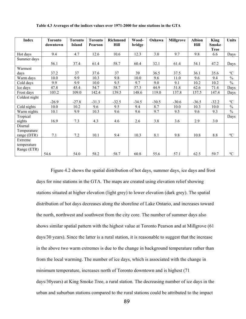
89

Table 4.3 Averages of the indices values over 1971-2000 for nine stations in the GTA

Figure 4.2 shows the spatial distribution of hot days, summer days, ice days and frost

days for nine stations in the GTA. The maps are created using elevation relief showing

stations situated at higher elevation (light grey) to lower elevation (dark grey). The spatial

distribution of hot days decreases along the shoreline of Lake Ontario, and increases toward

the north, northwest and southwest from the city core. The number of summer days also

shows similar spatial pattern with the highest value at Toronto Pearson and at Millgrove (61

days/30 years). Since the latter is a rural station, it is reasonable to suggest that the increase

in the above two warm extremes is due to the change in background temperature rather than

from the local warming. The number of ice days, which is associated with the change in

minimum temperature, increases north of Toronto downtown and is highest (71

days/30years) at King Smoke Tree, a rural station. The decreasing number of ice days in the

urban and suburban stations compared to the rural stations could be attributed to the impact

Index Toronto downtown

Toronto Island

Toronto Pearson

Richmond Hill

Wood-bridge

Oshawa Millgrove Albion Hill

King Smoke Tree

Units

Hot days 9.4 4.7 12.6 10.6 12.3 3.0 9.7 9.8 6.6 Days Summer days

56.1 37.4 61.4 58.7 60.4 32.1 61.4 54.1 47.2

Days Warmest days 37.2 37 37.6 37 39 36.5 37.5 36.1 35.6

ºC

Warm days 10.0 9.9 10.3 9.8 10.0 9.6 11.0 9.6 9.4 % Cold days 9.9 9.9 10.0 9.5 9.7 9.0 9.1 10.2 10.2 % Ice days 47.8 45.4 54.7 58.7 57.3 44.9 51.8 62.6 71.4 Days Frost days 103.2 109.0 142.4 139.5 148.6 119.0 137.8 157.5 147.4 Days Coldest night

-26.9 -27.8 -31.3 -32.5 -34.5 -30.5 -30.6 -36.5 -32.2

ºC Cold nights 10.0 10.2 9.6 9.5 9.4 8.7 10.0 10.3 10.0 % Warm nights 10.1 9.9 10.3 9.6 9.6 9.7 9.5 9.6 9.3 % Tropical nights 16.9 7.3 4.3 4.6 2.6 3.8 3.6 2.9 3.0

Days

Diurnal Temperature range (DTR) 7.1 7.2 10.1 9.4 10.3 8.1 9.8 10.8 8.8

ºC Extreme temperature Range (ETR)

54.6 54.0 58.2 58.7 60.8 55.6 57.1 62.5 59.7

ºC

90

of urbanization since urban heat island (UHI) is more pronounced on the minimum

temperature than on the maximum temperature (Chapter 2). Although it is not an established

fact that UHI has an impact on the changes in extreme temperatures, it is plausible that

higher temperature in urban areas may indirectly create a positive feedback for the frequency

of warm extremes (Cynthia et al, 2005). The lack of available moisture in paved urban areas

generates greater evaporative demand, which act as a positive feedback to increase the

intensity and frequency of the heat related extremes. Radiant energy from the sun is used at

the surface to either heat the surface, evaporate water or heat the subsurface (ground storage).

In urban settings a reduction in energy partitioned into latent heat of evaporation serves to

increase surface and subsurface heating. This is not the case for the rural areas with less

concrete; therefore, the frequency and duration of warm extremes are likely to be higher in

urban areas compared to a non-urban setting. Studies on heat related extremes for Toronto

and some other cities in Southern Ontario also suggested that the frequency and duration of

heat related event were more pronounced in areas with high levels of urbanizations (Smoyer

et al., 2000; Smoyer et al, 2003).

The number of frost days also shows a similar spatial pattern as ice days but with

the highest value at Albion Hill, which is probably due to the higher elevation of this station

compared to the others in the GTA. The warmest day and coldest night show consistent

spatial changes in temperature throughout the region. The WSDI and CSDI extreme indices

are also considered in this study, and are useful indicators for detecting warm spells and cold

spells during a particular time period. It is found that during 1971-2000, the WSDI was the

highest in 1973 with an average of 11 episodes throughout the GTA, followed by 1991, 1975,

1976 and 1998. The warmest day time is found to be in the year of 1988 with the highest

regional average maximum temperature of 37ºC, which is not associated with any of the

91

WSDI years with maximum events. To see whether there is a link between the WSDI and the

warmest day temperature, a correlation analysis is done between these two indices. The

results suggest that there is a weak positive correlation between WSDI and warmest days at

all stations except Richmond Hill for the period of 1971-2000. This is expected because

WSDI considers 6 consecutive days per year, which may not represent the warmest day time

every year. Therefore, the years with the highest events of WSDI cannot be entirely

attributed to the warmest day time during the 30 year period. Similarly with the minimum

temperature, the correlation analysis between the CSDI and the coldest nighttime temperature

show weak positive correlation at all stations, which indicate that highest CSDI events is not

entirely from the coldest nighttime temperature for the period of 1971-2000. For example,

the coldest nighttime of -31.5ºC is experienced in 1981 in the GTA, while the highest

episodes (8) of CSDI occurred in 1979.

92

93

Figure 4.2 Spatial distribution of hot days, summer days, ice days and frost days in the GTA. The circles are proportional to the magnitude of the average number of days for the period of 1971-2000. The average number of days per year is indicated inside the circles.

94

4.3.2 Analysis of annual extreme trends

Table 4.4 summarizes the results from the Mann-Kendall trend test and the TSA

method for all stations in the GTA. Contrary to the trends in daily minimum temperature,

fewer significant trends are observed for daily maximum temperature. The trends for indices

associated with minimum temperature are also more consistent throughout the GTA

compared to that of the maximum temperature. Hot days and summer days have non-

significant positive trends for most of the stations except the two rural stations, Albion Hill

and King Smoke Tree. Among the percentile based indices, the most pronounced changes are

observed for extreme cold days and cold nights. The former shows a decreasing trend for all

stations with statistically significant trends for Toronto Pearson, Richmond Hill and

Woodbridge. For the latter, five out of nine stations show significant negative trends in the

percentage of cold nights. The percentage of warm night shows non-significant positive

trends throughout the GTA, indicating that the region has experienced more warm nights and

fewer cold nights during 1971-2000. Most of the stations exhibit decreasing trends for DTR

and ETR with only exception being Millgrove. Ice days and frost days also show decreasing

trends for all stations, with statistically significant negative trends for frost days at Toronto,

Toronto Pearson and Woodbridge. Vincent and Mekis (2006) also found that there have been

significant decreases in frost day occurrence throughout Canada for the period of 1950-2003.

It is apparent from the trend analysis that certain trends in extreme temperature

indices (cold days, cold nights, ice days, frost days) are consistent with the expectations from

a greenhouse-gas induced climate change, while some (hot days, summer days, DTR)

suggest that other physical mechanisms such as the effect of urban warming, impact of local

topography are also at work at some of the stations in the GTA. For example, extreme hot

days and summer days have increasing trends at the urban and suburban stations but

95

decreasing trends at the rural stations, Albion Hill and King Smoke Tree. In general, the

temperature change in a rural setting is likely due to the changes in background temperature,

while in an urban setting it is due to both background temperature change and urban

warming. Therefore, the observation for the extreme hot days and summer days can be

attributed from the fact that the UHI has a positive feedback (explained in section 4.3.1) on

the temperature change at the urban and suburban stations, while at the rural stations, Albion

Hill and King Smoke Tree, the signal of urbanization is not present for the period of 1971-

2000 (Chapter 2). To summarize, the results from the trend analysis translate into more

significant trends in cold extremes compared to warm extremes, and the former shows

decreasing trends while the latter is associated with increasing trends for most of the stations.

This result is in agreement with the observation that the largest increases in daily maximum

and minimum temperature are occurring in cooler part of the years in Canada for the past few

decades (Robeson, 2004).

Figure 4.3 shows the spatial distribution of the trends obtained from the TSA

method for indices based on daily maximum, minimum and both temperatures. In case of

warm extremes, the magnitudes of the trends are greater at the centre of the GTA region,

particularly at Toronto Pearson and at Richmond Hill, for which the trends are also more

significant. For cold extremes the magnitude of the trends are more or less coherent

throughout the region except for frost days, which shows a significant decrease at the urban

and suburban stations. The spatial distribution of the trends in DTR is less consistent for the

stations in the GTA compared to that of the ETR. For DTR decreasing trends are evident at

most stations with the exception of the rural stations. Higher magnitude of trends (negative)

for DTR and ETR are more obvious at the urban and the suburban stations.

96

Table 4.4 Estimated trends for the annual extreme temperature indices for the period of 1971-2000 from the TSA analysis indicating the significant positive (+) and negative (−) trends in the GTA (no trend indicate an estimated slope of “0”)

Index Toronto downtown

Toronto Island

Toronto Pearson

Richmond Hill

Woodbridge Oshawa Millgrove Albion Hill

King Smoke Tree

Hot days + no trend + + no trend no trend + − * − Summer days + no trend + + + + * + − −

Warmest days − − + + no trend − + *− −

Warm days + + + + + + *+ − + Cold days − − * − * − * − − − − − Ice days − − − − *− no trend − − *− Frost days * − − *− − *− − − − − Coldest night no trend no trend + + + + + + +

Cold nights − − *− *− *− *− + *− − Warm nights + + *+ + + *+ + + *+

Tropical nights + + + + no trend *+ no trend + +

Diurnal Temperature range (DTR)

− no trend − − − − + *− no trend

Extreme temperature Range (ETR)

− − − − − no trend + − −

* Significant at 95%

97

98

99

Figure 4.3 (a) Trends in indices based of daily maximum temperature (hot days, summer days, warmest days, warm days, cold days and ice days) for the period of 1971-2000. The positive and negative signs inside the squares indicate increasing and decreasing trends, respectively and the blank ones represent no trend. The squares are proportional to the magnitude of the trends and the shaded squares represent significant trends.

100

101

102

Figure 4.3 (b) Same as 4.3a, only for indices based on daily minimum temperature

(cold nights, coldest nights, warm nights, tropical nights, frost days)

103

Figure 4.3 (c) Same as 4.3a, only for the indices based on both maximum and minimum temperatures (diurnal temperature range and extreme temperature range)

104

4.3.3 Analysis of seasonal extreme trends

The examination of extreme seasonal trends can be useful to determine if the

observed trends in annual temperature extremes are due to changes in a particular season.

Toronto experiences four distinct seasons that are defined as winter (December-February),

spring (March-May), summer (June-August) and autumn (September-November). Table 4.5

provides the results from the Mann-Kendall test and the TSA method showing significant

negative and positive trends for four seasons and for four temperature extremes, warm days,

warm nights, cold days and cold nights. Similar to the annual trends, there are more

significant trends for indices based on daily minimum temperature compared to the ones

based on daily maximum temperature, which are concentrated in winter and spring seasons.

Most of the stations in the GTA showed statistically significant increasing trends for the

percentage of warm days and warm nights in winter. Spring also shows a similar pattern.

However, for summer and autumn, the trends for warm days and warm nights are variable

throughout the region. On the contrary, the percentage of cold days is decreasing in all

seasons in the GTA, and the percentage of cold nights is decreasing in winter, spring and

summer. The trends in autumn are variable for cold nights. These observations are consistent

with the findings that there are fewer cold extremes in winter, spring and summer in most

parts of southern Canada, and more high temperature extremes in winter and spring for the

period of 1900-1998 (Bonsal et al., 2001). It seems that the increase in the percentage of

warm days is due to the increase in extreme hot days in winter and spring and also due to less

extreme cold days in winter, spring, summer and autumn. The increase in nighttime warming

in the GTA is mainly attributable to the increase (decrease) in warm night (cold night) in

winter, spring and summer, and to a lesser extent, to autumn, for which the observed indices

show variability within the region.

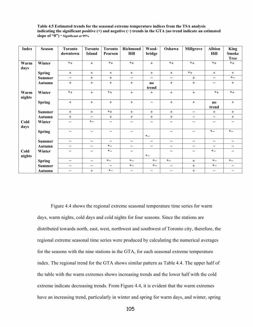
105

Table 4.5 Estimated trends for the seasonal extreme temperature indices from the TSA analysis indicating the significant positive (+) and negative (−) trends in the GTA (no trend indicate an estimated slope of “0”) * Significant at 95%

Figure 4.4 shows the regional extreme seasonal temperature time series for warm

days, warm nights, cold days and cold nights for four seasons. Since the stations are

distributed towards north, east, west, northwest and southwest of Toronto city, therefore, the

regional extreme seasonal time series were produced by calculating the numerical averages

for the seasons with the nine stations in the GTA, for each seasonal extreme temperature

index. The regional trend for the GTA shows similar pattern as Table 4.4. The upper half of

the table with the warm extremes shows increasing trends and the lower half with the cold

extreme indicate decreasing trends. From Figure 4.4, it is evident that the warm extremes

have an increasing trend, particularly in winter and spring for warm days, and winter, spring

Index Season Toronto downtown

Toronto Island

Toronto Pearson

Richmond Hill

Wood-bridge

Oshawa Millgrove Albion Hill

King Smoke Tree

Warm days

Winter *+ + *+ *+ + *+ *+ *+ *+

Spring + + + + + + *+ + + Summer − + + − − − + − *− Autumn + + + + no

trend + + − +

Warm nights

Winter *+ + *+ + + + + *+ *+

Spring + + + + − + + no trend

+

Summer + + *+ + + + − + + Autumn + − + + + + − − + Cold days

Winter − *− − − − − − − −

Spring − − − − *−

− − *− *−

Summer − − − − − − − − − Autumn − − *− − − − − − − Cold nights

Winter − − *− − *−

− − *− −

Spring − − *− *− *− *− + *− *− Summer − − − *− *− − + *− − Autumn − + *− − − − + − −

106

and summer for warm nights. The trend in autumn is not coherent for any of the warm

extremes. The increasing trend for warm days and warm nights vary from 7 to12 percent

indicating that there are 25 to 43 more warm days and warm nights per year for the GTA

region during 1971-2000. The regional pattern for cold extremes also shows the same

seasonal distribution that is a decreasing trend for cold days in winter and summer, and for

cold nights in winter, spring and summer. The downward trend for the cold extremes

fluctuates around 6 to 13 percent, which signifies that there are 22 to 47 fewer cold days or

cold nights per year throughout the region, particularly in winter and spring, during the 30

years period. Similar results were found from another study on Canada for the period of

1900-2003, which showed that there are 28 fewer cold nights, 10 fewer cold days, 21 more

warm nights, and 8 more hot days per year in recent years than in 1900 (Vincent and Mekis,

2006). It is also evident from Figure 4 that the increasing (decreasing) trend for warm (cold)

extremes are more evident in the latter part of the period, particularly during 1991-2000.

107

A) Warm Days

Winter

0.0

5.0

10.0

15.0

20.0

25.0

1971

1973

1975

1977

1979

1981

1983

1985

1987

1989

1991

1993

1995

1997

1999

Years

Perc

ent o

f day

s

Spring

0.0

5.0

10.0

15.0

20.0

25.0

1971

1973

1975

1977

1979

1981

1983

1985

1987

1989

1991

1993

1995

1997

1999

Years

Perc

ent o

f day

s

Summer

0.0

5.0

10.0

15.0

20.0

25.0

30.0

1971

1973

1975

1977

1979

1981

1983

1985

1987

1989

1991

1993

1995

1997

1999

Years

Perc

ent o

f day

s

Autumn

0.0

5.0

10.0

15.0

20.0

25.0

1971

1973

1975

1977

1979

1981

1983

1985

1987

1989

1991

1993

1995

1997

1999

Years

Perc

ent o

f day

s

108

B) Warm Nights

Winter

0.0

5.0

10.0

15.0

20.0

25.0

1971

1973

1975

1977

1979

1981

1983

1985

1987

1989

1991

1993

1995

1997

1999

Years

Perc

ent o

f day

s

Spring

0.0

5.0

10.0

15.0

20.0

25.0

30.0

1971

1973

1975

1977

1979

1981

1983

1985

1987

1989

1991

1993

1995

1997

1999

Years

Perc

ent o

f day

s

Summer

0.0

5.0

10.0

15.0

20.0

25.0

1971

1973

1975

1977

1979

1981

1983

1985

1987

1989

1991

1993

1995

1997

1999

Years

Perc

ent o

f day

s

Autumn

0.0

5.0

10.0

15.0

20.0

25.0

1971

1973

1975

1977

1979

1981

1983

1985

1987

1989

1991

1993

1995

1997

1999

Years

Perc

ent o

f day

s

109

C) Cold Days

Winter

0.0

5.0

10.0

15.0

20.0

25.0

1971

1973

1975

1977

1979

1981

1983

1985

1987

1989

1991

1993

1995

1997

1999

Years

Perc

ent o

f day

s

Spring

0.0

5.0

10.0

15.0

20.0

1971

1973

1975

1977

1979

1981

1983

1985

1987

1989

1991

1993

1995

1997

1999

Years

Perc

ent o

f day

s

Summer

0.0

5.0

10.0

15.0

20.0

25.0

30.0

35.0

1971

1973

1975

1977

1979

1981

1983

1985

1987

1989

1991

1993

1995

1997

1999

Years

Perc

ent o

f day

s

Autumn

0.0

5.0

10.0

15.0

20.0

25.0

1971

1973

1975

1977

1979

1981

1983

1985

1987

1989

1991

1993

1995

1997

1999

Years

Perc

ent o

f day

s

110

D) Cold Nights

Winter

0.0

5.0

10.0

15.0

20.0

25.0

1971

1973

1975

1977

1979

1981

1983

1985

1987

1989

1991

1993

1995

1997

1999

Years

Perc

ent o

f day

s

Spring

0.0

5.0

10.0

15.0

20.0

1971

1973

1975

1977

1979

1981

1983

1985

1987

1989

1991

1993

1995

1997

1999

Years

Perc

ent o

f day

s

Summer

0.0

5.0

10.0

15.0

20.0

25.0

1971

1973

1975

1977

1979

1981

1983

1985

1987

1989

1991

1993

1995

1997

1999

Years

Perc

ent o

f day

s

Autumn

0.0

5.0

10.0

15.0

20.0

25.0

1971

1973

1975

1977

1979

1981

1983

1985

1987

1989

1991

1993

1995

1997

1999

Years

Perc

ent o

f day

s

Figure 4.4 Extreme temperature indices for seasonal temperature time series for the GTA. The linear trend is shown by the bold line. A) Warm Days, B) Warm Nights, C) Cold Days and D) Cold Nights

111

4.3.4 Analysis of economically significant indices

The final phase of this chapter is based on economically sensitive indices, heating

degree days and cooling degree days, which are related to the observed changes in daily

mean temperature in the GTA. Due to their significance, economically and socially, these

indices are explored separately and their changes are related to urban heat island. Changes in

both HDD and CDD can affect human comfort and energy consumption. The urban

warming has major impact on the nighttime temperature increase (Chapter 2), which can

reduce the comfort level for sleeping and thus can increase the requirement for more air

conditioning. The decrease in HDD would reduce energy consumptions in winter, which may

seem economically beneficial in energy demand context. However, mild winters with less

snow may seriously affect winter tourism due to the reduction of outdoor recreation activities

such as ice fishing, skiing, snowboarding etc.

The changes in HDD and CDD is examined by considering two different time

periods, 1971-2000 and 1991-2000 in order to compare the changes with the pace of

urbanization. Figure 4.5 compares the variation of HDD and CDD for the two periods. It is

apparent from the figure that there is a substantial decrease in heating degree days during

1991-2000 compared to 1971-2000. The decrease in HDD is evident in all stations

throughout the GTA except Millgrove. Contrary to heating degree days, the increase in

cooling degree days is not obvious at all stations. The cooling degree days have increased

during 1991-2000 compared to 1971-2000, mainly at urban and suburban stations, including

Toronto Pearson, Richmond Hill, Woodbridge and Oshawa. This observation can be

attributable to the increase in minimum temperature during 1989-2000 compared to 1970-

2000 in the above stations (Chapter 2, figure 2.5). The changes in CDD are not obvious for

Toronto downtown, Toronto Island and the rural stations. The former two stations are

112

situated by Lake Ontario, and experience a mitigating effect on their temperature changes,

particularly during the warmer months of the year (Chapter 2). Similar to other studies

(Todhunter, 1996; Cartalis et al., 2001; Baker et al., 2002), the higher magnitudes of HDD

and CDD are more obvious at stations, which experienced most urbanization impacts during

the specified study periods. For example, the decrease in HDD and increase in CDD are more

prominent at Toronto Pearson and Richmond Hill compared to the other stations. This is

consistent with the fact that the suburban fringe of the study has started to manifest the

urbanization signal and the associated warming (Chapter 2).

113

HDD

3200

3400

3600

3800

4000

4200

4400

Torond

own

ToronIs

land

ToronP

earso

n

Richmon

d Hill

Woo

dbrid

ge

Oshaw

a

Millgrov

e

Albion

Hill

King S

moke T

ree

Sum

of h

eatin

g de

gree

day

s, ºC

91-0071-00

CDD

150

200

250

300

350

400

Toron

down

Toron

Islan

d

Toron

Pearso

n

Richmon

d Hill

Woo

dbrid

ge

Oshaw

a

Millgrov

e

Albion

Hill

King S

moke T

ree

Sum

of c

oolin

g de

gree

day

s, ºC

91-0071-00

Figure 4.5 Comparison of the differences in average heating degree days (HDD) and cooling degree days (CDD) for two different periods, 1971-2000 and 1991-2000.

114

In order to take a more detailed look at the changes in HDD and CDD, their trends are

analyzed using the results from Mann-Kendall test and TSA approach for the two periods,

and are presented in Table 4.6.

Table 4.6 Comparison of the trends for HDD and CDD between 1971-2000 and 1990-2000

as derived from Theil-Sen slope estimator (degree days/year)

Stations HDD CDD 1971-2000 1991-2000 1971-2000 1991-2000 Toronto downtown -8.8 -29 0.7 -1 Toronto Island -11.6* -14.7 0.9 -0.7 Toronto Pearson -19.4* -18.4 3.7* 9.3 Richmond Hill -9.8* -19 1.8 -4.5 Woodbridge -17.8* 10.5 1.7 9.3 Oshawa -7.5 -25.8 1.1 -1.9 Millgrove 2.0 -38.3 1.3 5.8 Albion Hill -23.5* -87.3 0 -7.1 King Smoke Tree -27* -36 -0.3 2.8 *Statistically significant at 95% level

The results from the trend analysis suggest that a decrease in HDD occurs at every station in

the GTA for both periods. However, the trends for HDD are statistically significant mainly

for the period of 1971-2000. Although none of the HDD trends are significant from 1990-

2000, the decrease in magnitude of the annual HDD is much higher during this period,

particularly at Toronto downtown, Albion Hill and King Smoke Tree. The trend results for

HDD are fairly consistent with the study of HDD at selected Southern Ontario locations

conducted by Klaassen (2003). This study has three stations in common with the Klaassen

study, Toronto downtown, Toronto Pearson and Richmond Hill, for which seven different

periods were considered. Although the study used best-fit linear regression to estimate the

trend instead of Mann-Kendall test, the significance of the trend results are similar for the

common stations for similar periods of study, 1960-2001 and 1990-2001. For the former

period the trends were significant for the three stations, while for the latter the trends were

non-significant. A similar study on HDD and CDD was performed by Bonsal et al. (2001),

which suggested a decrease in HDD, at every station within southern Canada (south of 60ºN)

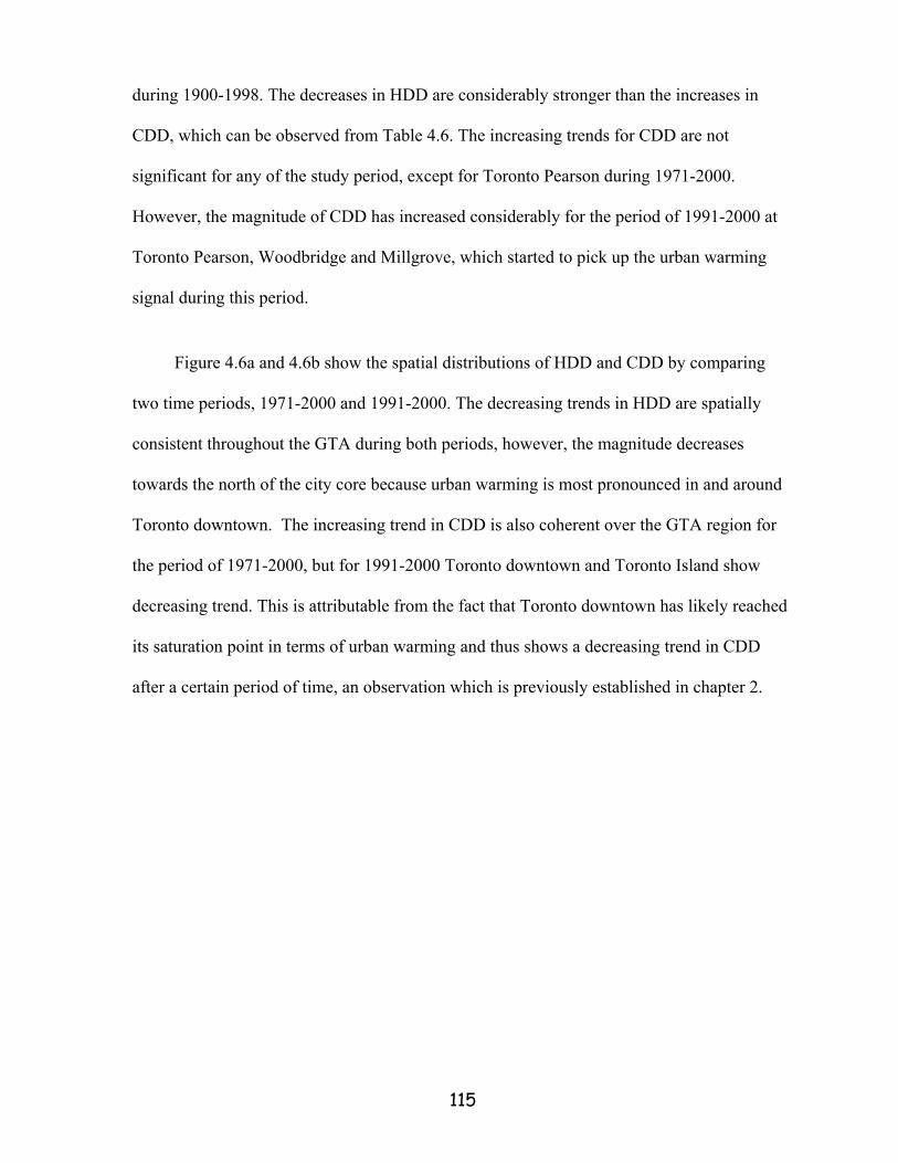
115

during 1900-1998. The decreases in HDD are considerably stronger than the increases in

CDD, which can be observed from Table 4.6. The increasing trends for CDD are not

significant for any of the study period, except for Toronto Pearson during 1971-2000.

However, the magnitude of CDD has increased considerably for the period of 1991-2000 at

Toronto Pearson, Woodbridge and Millgrove, which started to pick up the urban warming

signal during this period.

Figure 4.6a and 4.6b show the spatial distributions of HDD and CDD by comparing

two time periods, 1971-2000 and 1991-2000. The decreasing trends in HDD are spatially

consistent throughout the GTA during both periods, however, the magnitude decreases

towards the north of the city core because urban warming is most pronounced in and around

Toronto downtown. The increasing trend in CDD is also coherent over the GTA region for

the period of 1971-2000, but for 1991-2000 Toronto downtown and Toronto Island show

decreasing trend. This is attributable from the fact that Toronto downtown has likely reached

its saturation point in terms of urban warming and thus shows a decreasing trend in CDD

after a certain period of time, an observation which is previously established in chapter 2.

116

Figure 4.6 (a) Spatial comparison of the changes in HDD between 1971-2000 and 1991-2000 (positive sign indicates increasing trend and negative sign indicates negative trends)

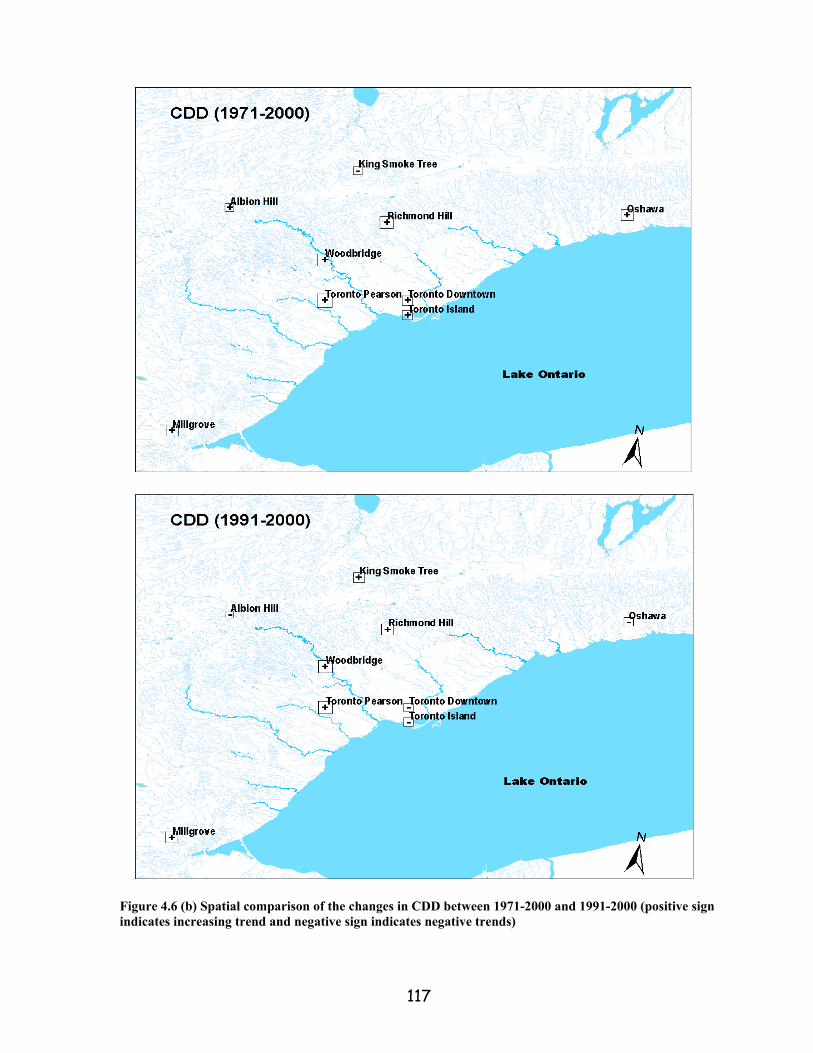
117

Figure 4.6 (b) Spatial comparison of the changes in CDD between 1971-2000 and 1991-2000 (positive sign indicates increasing trend and negative sign indicates negative trends)

118

4.4 Summary and conclusions

This chapter examined the changes in extreme indices and their trends for daily

maximum and minimum temperature observed in the GTA for the period of 1971-2000. The

changes in indices that are based on daily maximum temperature (hot days, summer days) are

more pronounced at the urban and suburban stations compared to the stations situated at the

shoreline of Lake Ontario and at the rural station, King Smoke Tree. The percentile based

indices including warm days, cold days, warm nights and cold nights are found to be

consistent around 10 percent for nine stations throughout the GTA. The results from the trend

analysis revealed no significant changes in the indices based on daily maximum temperature,

although they show increasing trends for all stations except the rural stations, Albion Hill and

King Smoke Tree. The spatial distribution of the warm extremes shows similar pattern as the

temporal trends, including more ice days and frost days at the rural stations as opposed to the

urban and the suburban stations. Since rural settings are likely only affected by the

background temperature change, therefore, the above observation is indicative of the fact that

local warming could act as a positive feedback on the extreme temperature change. In other

words, the urban warming related to UHI may have paved the way to extend the spatial and

temporal dimensions of extreme temperature changes due to the urban-suburban heat

exchange complex compared to the heat exchange phenomenon in the rural surrounding

(Cynthia et al., 2005). The indices based on daily maximum temperature have non-significant

increasing trends at most stations. The indices based on daily minimum temperature (cold

days, cold nights) exhibit significant decreasing trends irrespective of the impact of local

effect at the individual station. The coldest night of the year is also getting warmer, and there

are more events of warm spells compared to cold spells over the GTA. The temporal and

119

spatial distributions of cold extreme indices are more coherent throughout the region

compared to the warm extreme indices.

The results from the trend analysis of seasonal extreme temperature for warm

days, warm nights, cold days and cold nights suggest consistent trends for all stations. There

are statistically significant trends toward more days with extreme high temperature in winter

and spring, but no indication of any significant trend of extreme high temperature in summer.

The trends in warm days for autumn show variability within the region. The percentage of

cold night has decreasing trends in winter, spring and summer while the percentage of warm

night has increasing trends for the same seasons. The significant decrease in diurnal

temperature range is, therefore, due to the nighttime warming over the GTA region, which is

also favorable under UHI related phenomenon. The analysis of the regional trends in

seasonal extreme indices revealed that the above changes in cold and warm extremes were

more evident during the last 10 years of the study period, that is, during 1991-2000. To

summarize, the results from the analysis of extremes indices for daily maximum and

minimum temperature suggest that there is a shift towards warmer climate in the GTA region

with an increase in extreme high temperature and a reduction in extreme low temperatures

during daytime. These changes have been especially apparent in winter and spring compared

to summer and autumn. Regarding the extreme nighttime temperature, fewer nights with

extreme low nighttime temperature were observed in summer and more nights with extreme

high nighttime temperature were found in all seasons.

Finally, the temporal and spatial analysis of the economically important indices, heating

degree days and cooling degree days, revealed that the former is associated with a decreasing

trend at all stations except Millgrove and the latter exhibited increasing trends at all stations

120

except at King Smoke Tree. The magnitude of the trends for HDD and CDD are higher

during 1991-2000 compared to 1971-2000. This observation is an indication of urban

warming, particularly at the suburban stations, which started to manifest the urbanization

signal during the latter period. The heating and cooling degree days are principal indicators

of energy demand and human comfort, which in turn have an impact on the energy sector.

In conclusion, this chapter provides valuable insights on the changes in extreme

indices of daily maximum and minimum temperature in the GTA region for the first time.

The majority of the results are consistent with the expectations of a warming climate, except

the lack of significant changes to extreme high temperature in summer. Understanding of the

changes in extremes provides basis for establishing the cause and effect relationships, which

are critical for the attribution of climate change to human activities. Future research need to

incorporate more areas in Ontario to examine the regional trends and variability in

temperature extremes.

121

Chapter 5: Discussion and Conclusions The central objective of this dissertation was to analyze the climate change and

variability in the GTA in the context of the urban heat island. Non-parametric statistical

techniques such as sequential Mann-Kendall test, Mann-Kendall trend estimation of

Kendall’s tau, and Theil-Sen approach of slope estimation are used for the analysis of

temperature time series in this thesis. The procedural methods in this research are similarly

applicable in any part of the world. With an aim to understanding the impact of UHI effect on

the temperature changes, in chapter 2 as a first step, the annual and seasonal temperature time

series (31-162 years) were analyzed using several meteorological stations in the GTA. The

results from Mann-Kendall test and Theil-Sen slope estimation revealed statistically

significant increase of annual mean and minimum temperature at almost all stations. The

maximum temperature trends were significant at 99% level only at the suburban stations. In

terms of seasonal trends, winter was found to have the clearest change signal, and thus

contributed substantially to the increase in annual minimum temperature. The analysis of the

linkage between the urbanization and temperature changes during the 1970-2000 period

indicated that the stations in the GTA exhibited substantial departures from Toronto

downtown temperatures in all habitable directions including east, west and north of Toronto

which extended beyond 50 km from the city core. The sequential Mann-Kendall test, which

was used to detect abrupt climate change, suggested that the increase in annual mean

temperature started after 1920 at Toronto downtown, after the 1960s at the suburban stations,

and increased significantly during the 1980s at all stations. Thus the outcomes from the

Mann-Kendall test were further verified by the sequential Mann-Kendall test. The results

from the three tests collectively were very useful in specifying a period, which was found to

122

be 1980s, during which the impact of UHI was most pronounced in the GTA. A comparison

of the trends between Toronto and a rural station confirmed the above observation, which

suggested that during 1980-2006 the UHI impact had extended beyond the city core and was

more pronounced on the suburban fringe in the GTA, and the effect was more evident on the

minimum temperature compared to that on the maximum temperature changes. The results

from the trend analysis thus, provided the genesis toward the assessment of UHI impact on

temperature changes in the GTA. The findings are applicable to mid-to-high latitude cities,

particularly for urban areas with similar geographic and climatic characteristics as Toronto.

Future studies should include a larger network of meteorological stations, and should

incorporate the effect of synoptic conditions, which will be able to provide more

comprehensive measures of urbanization impacts at both local and regional scales.

The results from chapter 2 motivated the analysis that was carried out in chapter 3,

which was the estimation and characterization of Toronto’s UHI with the purpose to identify

the impact of the selection of rural sites on the estimation of UHI intensity. Three rural

stations King Smoke Tree (KST), Albion Hill and Millgrove, situated towards north,

northwest and southwest of Toronto, respectively, were used for the estimation of UHI

intensity (∆Tu-r) for two urban stations, Toronto downtown and Toronto Pearson using data

from 1970 to 2000. The rural stations have different climatic characteristics in terms of

different land use type, location relative to the urban station and topography (e.g. the effect of

water body, elevation etc.). The ∆Tu-r computed for both Toronto and Pearson were

characterized as: winter dominating and summer dominating depending on the choice of the

rural station. The former was observed when ∆Tu-r was estimated using KST and Millgrove,

and the latter was observed with Albion Hill. The analyses of annual, seasonal and diurnal

123

trends of ∆Tu-r suggested that urban heat island clearly appears in winter at both Toronto and

Pearson. Therefore, Albion Hill was suggested to be a less suitable choice as a rural station,

with which both urban stations showed summer dominating UHI intensity. Using KST,

which is further inland relative to Toronto, the trend in UHI intensity during 1970-2000 was

underestimated compared to the value reported by IPCC (0.006°C/decade) for the Northern

Hemisphere. If Millgrove was used, which is situated near the lake as Toronto, then the trend

in UHI intensity was in good agreement with the IPCC value. However, with Pearson with

no direct lake effect, KST was more appropriate than Millgrove. Thus the current study

suggests that the choice of a pair to estimate ∆Tu-r is dependent on the topographic and

climatic characteristics of urban and rural stations, and also more importantly on the

objective of a particular study in the context of UHI intensity. In addition, it is proposed that

the selection process of a pair of urban-rural station to estimate ∆Tu-r, which is in practice in

the current urban climate literature, need to adopt a more comprehensive approach. The

proper definitions of urban and rural stations need to be quantified. Instead of using single

criteria to identify the type of a station, the use of more than one feature will facilitate the

selection of a suitable urban-rural pair. For example, using a combination of physical and

climatic characteristics, population distribution and satellite night-light data to identify urban

and rural stations is a more appropriate choice to select an urban-rural pair compared to using

one characteristic to choose the pair. This study provided important criteria in choosing a

rural station, particularly for cities with similar topographic characteristics as Toronto, and

suggested that it is imperative to choose urban-rural station pair from a clear, objective and

climatologically significant standpoint. Moreover, an important message emerged from this

study was that proper identification of urban-rural dichotomy is one of the current challenges

in urban climate literature, and is fundamental to UHI definition, experimentation and

124

quantification. It is imperative to set a standard or rules to identify urban-rural pair, by the

scientific community associated with urban climate research, which can be used universally

for UHI study. The research approach used in chapter 3 is applicable to any city, which

experiences climate conditions arising from urbanization related phenomena.

In chapter 4, the analysis of the trends in the extreme temperature indices were

presented for daily maximum and minimum temperature observed in the GTA for the period

of 1971-2000. Warm extremes, which are based on daily maximum temperature such as hot

days, summer days, were more pronounced at the urban and suburban stations, compared to

the rural stations. Cold extremes, which are based on daily minimum temperature, showed

coherent changes throughout the GTA. More significant trends were observed for the cold

extremes compared to that for warm extremes. This observation is consistent with the results

from chapter 2, which confirmed the fact that the dominant effect of urban heat island was on

the minimum temperature rather than on the maximum temperature. For example, for

extremes based on minimum temperature such as the decreasing number of frost days in

urban and suburban stations compared to the rural stations could be attributed to the impact

of urbanization. Significant impact of urbanization is also evident on the two economically

important indices, heating degree days and cooling degree days. Because of urban warming,

the trend in heating degree days is decreasing while that for cooling degree days is

increasing, particularly at the urban and suburban stations in the GTA. The changes in HDD

and CDD are also more pronounced during 1991-2000 compared to 1971-2000. Due to

higher nighttime temperatures there is continuous use of air-conditioners in cities, which

results in higher demand of energy. This was not the case several decades ago when

nighttime temperatures were cool enough to sleep with open windows. Since the urban

fringes are now extended further away and are replaced by suburban fringes, the nighttime

125

cooling from country breezes are not there. Instead warm air flow within the urban-suburban

closed circulation system is the dominant phenomenon, which is the primary cause of

nighttime temperature increases in cities.

To summarize, the key finding of this dissertation was that the trends of both annual

temperature and their extreme indices have changed in the GTA during 1970-2000. During

this period the UHI effect has contributed at least one third to the observed annual warming.

There were increases in the percentage of warm days and warm nights and decreases in the

percentage of cold days and cold nights. The analyses of temperature and the changes in

extremes in the GTA thus manifest a shift towards a warmer climate with an increase in

annual mean and extreme high temperatures, and reduction in extreme low temperatures. The

intensity, duration, frequency and spatial extent of extremes changes, and future changes

associated with continued warming will present additional challenges on the urban climate

system. It is evident that the urban heat island phenomenon produces a warmer climate in

cities, and with the current pace of urbanization in the GTA, it is imperative to understand the

impact of the emerging UHI in the GTA in terms of human comfort, city water supply,

energy demand, and also air pollution. The urban climate change is an important driver of

these adverse effects.

The results from this dissertation provide important scientific evidence, which suggest

that urban heat island impact in cities is not a theoretical problem but is already underway. In

addition, global climate change is manifested on a local level by more variable weather

patterns and extreme events due to the effects from urban climate change. Cities like Toronto

with the high concentration of people, property and aging infrastructure are particularly

vulnerable to changes in climate and extreme weather under the current pace of urbanization.

126

For example, an increase in extreme weather events will damage property and infrastructure

and place a significant financial burden on the city. Moreover, Toronto’s natural ecosystem

already faces pressure from urban growth. The urban forest will suffer from the increase in

severity and duration of warm extremes, such as hot days and heat waves. An increase in heat

will also exacerbate air pollution, particularly ground level ozone, which is the primary

ingredient in smog. This will in turn affect the health of the residents in urban-suburban

areas. With the increase in wintertime temperature, vector-borne diseases will spread because

warmer weather allows carriers to expand their range and infectious agents to survive the

winter. Increase in summertime temperature will increase energy use, especially electricity,

which will be affected with the current pace of urbanization in terms of generation,

production and distribution. Energy demand is also expected to increase with the changes in

HDD and CDD, putting the entire system under greater strain. The impacts of the above

mentioned changes will reverberate with the urban sprawl leaving the socio-economic

condition in the GTA highly vulnerable to future climate change. Decision makers in both

the public and private sectors will need to assess the risks associated with the increase in

urbanization and the associated climate change, and take appropriate actions to better adapt

to the changes ahead.

Therefore, the forecasting of future climate change is essential from social and

economic standpoint in terms of infrastructure design and planning with ongoing

urbanization in the GTA. Future research needs to incorporate urban climate in forecasting

climate change by statistically downscaling climate model results to the local climate in

cities. Investigations of temperature and their extremes at local scales can also provide

important climatic genesis about how larger-scale atmospheric changes may influence the

climatologically sensitive parameters such as temperature. One of the challenges that was

127

experienced while performing this research was the scarcity of data in this region. More data

need to be collected and documented for longer-periods of time with careful attention

directed to the challenges of measuring in urban environment. Archiving of land use change

and land cover descriptions is vital along with the atmospheric data. In conclusion, more

integrative approaches into the attribution of current and future regional trends and variability

in temperature and the associated changes in their extremes are required by expanding

towards more areas and longer time period of analysis in the GTA, Ontario.

128

References Aesawy, A.M. & H. M. Hasanean, 1998. Annual and Seasonal Climatic Analysis of Surface

Air temperature Variations at six Mediterranean Stations. Theoretical and Applied

Climatology. 61, 55-68.

Ackerman, B., 1985. Temporal march of the Chicago heat island, Journal of Climate and

Applied Meteorology. 24, 547-554.

Adebayo, Y. R., 1991. Heat island in a humid tropical city and its relationship with potential

evaporation. Theoretical and applied climatology. 43, 137-147.

Arritt, R.W., 1987. The Effect of Water Surface Temperature on Lake Breezes and Thermal

Internal Boundary Layers. Boundary-Layer Meteorol. 40:101-125.

Atkinson, B. W. 1981. Meso-scale Atmospheric Circulations. Academic Press, London, 495

pp.

Augiliar, E. et al., 2005. Changes in precipitation and temperature extremes in Central

America and northern South America, 1961-2000, Journal of Geophysical Research. 110,

D23107,doi:10.1029/2005JD006119.

129

Baker, L. A., A. J. Brazel, N. Selover, C. Martin, N. McIntyre, F. R. Steiner, A. Nelson and

L. Musacchico, 2002. Urbanization and warming of Phoenix (Arizona, USA): Impacts,

feedbacks and mitigations. Urban Ecosystems, 6, 183-203.

Bonsal, B. R., X. Zhang, L. A. Vincent and W. D. Hogg, 2001. Characteristics of Daily and

Extreme Temperatures over Canada, Journal of Climate, 14, 1959-1976.

Böhm, R., 1998. Urban bias in temperature time series- A case study for the city of Vienna,

Austria. Climatic Change. 38,113-128.

Böhm, R., I. Auer, M. Brunetti, M. Maugeri, T. Nanni & W. Schöner, 2001. Regional

temperature variability in the European Alps: 1890-1998 from homogenized instrumental

time series. Int. Journal of climatology. 21, 1779-1801.

Bornstein, R. and Q. Lin, 2000. Urban Heat Islands and summertime convective

thunderstorms in Atlanta: Three case studies. Atmos. Environment, 34, 507-516.

Camilloni, I. & Barros, V., 1997. On the urban heat island effect dependence on temperature

trends. Climatic Change. 37, 665-681.

Cartalis, C., A. Synodinou, M. Proedrou, A. Tsangrassoulis and M. Santamouris, 2001.

Modification in energy demand in urban areas as a result of climate changes: an assessment

for the southwest Mediterranean region. Energy Conversion and Management, 42, 1647-

1656.

130

Changnon, S. A., R. G. Semonin and F.A. Huff, 1976. A hypothesis for urban rainfall

anomalies. J. of Applied Meteorology, 15, 544-559.

Canyon, D. R. and A. V. Douglas, 1984. Urban influence on surface temperature in the

southwestern United States during recent decades, J. of climate and Applied Meteorology.

23, 1520-1530.

Conrad, V. and C. Pollak, 1950. Methods in climatology. Harvard University Press,

Cambridge, MA. p. 459

Çiçek, İ. And U. Doğa, 2006. Detection of urban heat island in Ankara, Turkey. IL NUOVO

CIMENTO, 29 C (4), 399-409.

Cynthia, R., W. D. Solecki, L. Parshall, M. Chopping, G. Pope and R. Goldberg, 2005.

Characterizing the urban heat island in current and future climates in New Jersey,

Environmental Hazards, 6, 51-62.

Duchon, C. E., 1986. Temperature Trends at Sun Juan, Puerto Rico. Bull. of American

Meteorological Society. 67, 1370-1377.

Easterling, D. R., J. R. Evans, P. Ya. Groisman, T. R. Karl, K. E. Kunkel, and P. Ambenje,

2000. Observed variability and trends in extreme climate events: a brief review. Bulletin of

the American Meteorological Society, 81(3), 417-425.

131

Easterling, D.R., H. F. Diaz, A. V. Douglous, W. D. Hogg, K.E. Kunkel, J. C., Rogers and J.

F. Wilkinson, 1999. Long-term observations for monitoring extremes in the Americas,

Climatic Change, 42, 285-308.

Easterling, D.R., B. Horton, P.D. Jones, T.C. Peterson, T.R. Karl, D.E. Parker, M.J. Salinger,

V. Razuvayev, N. Plummer, P. Jamason and C.K. Folland, 1997: Maximum and minimum

temperature trends for the globe. Science, 277, 364-367.

Eliasson, I., 1994. Urban-suburban-rural air temperature differences related to street

geometry. Physical geography. 15, 1-22.

Folland, C.K. and Karl, T.R., 2001. Observed Climate Variability and Change. Pages 99-181

in Houghton, J. T., Ding, D. J., Griggs, M., Noguer, M., van der Linden, P.J., Dai, X.,

Maskell, K. and Johnson, C. A. (eds.). Climate change 2001: The Science of Climate

Change. Contribution of Working Group I to the third Assessment Report of the

Intergovernmental Panel on Climate Change. Cambridge University Press, Cambridge.

881pp.

Frich, P., L.V. Alexander, P. Della-Marta, B. Gleason, M. Haylock, A.M.G. Klein Tank, T.

Peterson, 2002. Observed coherent changes in climatic extremes during the second half of

the twentieth century, Climate Reserch, 10, 193-212.

Gargett, A., 1965. Long term fluctuations in the Toronto temperature and precipitation

record, Dept. of Transport, Meteorological Branch, Canada, 15p.

132

Gilman, C., Berger, A., 1986: Annual and seasonal climatic variations over the northern

hemisphere and Europe during the last century. Annals Geophys., 4b, 385-400.

Godowitch, J.M., J. K. S. Ching and J.F. Clarke, 1985. Evolution of the Nocturnal Inversion

Layer at an Urban and Nocturnal Location, J. Clim. Appl. Meteorol. 24, 791-804.

Gough, W. A., 2000. A climate perspective on the blizzard of ’99. CMOS Bulletin, 28:17.

Gough, W. A. and Y. Rozanov, 2001. Aspects of Toronto’s climate: heat island and Lake

Breeze. Canadian Meteorological Oceanographic Society Bulletin, 29, 67-71.

Gough, W.A., Lillyman, C., Karagatzides, J. and T.J.S. Tsuji, 2002. Determining the validity

of using summer monitoring to estimate annual deposition of acidic pollutants in southern

Ontario, Canada. Water, Air, and Soil Pollution 137, 305-316.

Gough, W.A., 2008. Theoretical considerations of day-to-day temperature variability applied

to Toronto and Calgary, Canada data. Theoretical and Applied Climatology 94, 97-105.

Harris, R. and M. Luymes, 1990. The Growth of Toronto, 1861-1941: A Cartographic Essay.

Urban History Review, XVIII, No 3, 244-255.

Hedquist, B.C. and A.J. Brazel,2006. Urban, residential and rural climate comparisons from

mobile transects and fixed stations: Phoenix, Arizona. J. Arizona-Naveda Acad. Sci. 38, 77-

87.

133

Helsel, D.R. & R.M. Hirsch, 1992. Statistical methods in water resources, Elsevier Science

Publishers, USA, 522p.

Hirsch, R. M.,J. R. Slack and R. A. Smith, 1982. Techniques of trend analysis for monthly

water quality data. Water Resources Research, 18, 107-121.

Hirt, M. S. and R. W. Shaw, 1973. The Passage of a lake-breeze front at Toronto- a

comparison between the city and the suburbs. Atmospheric Environment. Paragon Press. 7,

63-73.

Huff, F. A. and S. A.Changnon, 1973. Precipitation modification of major urban areas. Bull.

Amer. Meteor. Society, 54, 1220-1232.

Huff, F. A. and S. A.Changnon, 1972. Climatological assessment of urban effects on

precipitation at St. Louis. J. of applied Meteorology, 11, 823-842.

Jauregui, E., 1997. Heat Island Development in Mexico City. Atmospheric Environment. 31,

3821-3831.

Jones, P.D., P.Ya. Groisman, M. Coughlan, N. Plummer, W.C Wang, and T.R. Karl,

1990:Assessment of urbanization effects in time series of surface air temperature over land.

Nature, 347, 169-172.

Kadioğlu, M., 1997 Trends in surface air temperature data over Turkey. Int. Journal of

climatology. 17, 511-520.

134

Kadioğlu, M., Z. Şen and L. Gültekin, 2001. Variations and Trends in Turkish Seasonal

Heating and Cooling Degree-Days. Climatic Change. 49, 209-223.

Karl, T.R., H. F. Diaz & G. Kukla, 1988. Urbanization: Its detection and effect in the United

States climate record. Journal of Climate. 1,1099-1123.

Karl, T. R., P. D. Jones, R.W. Knight, G. Kukla, V. Plummer, Raxuvayev, K. P. Gallo, J.

Lindseay, R. J. Charleston and T. C. Peterson, 1993. Asymmetric trends of daily maximum

and minimum temperature, Bull. Am. Meteorol. Soc., 74 (6), 1007-1023.

Kalnay,E. and Ming Cai, 2003. Impact of urbanization and Land-use change on climate.

Nature. 423, 528-531.

Keen, C.S. and W.A. Lyons, 1978. Lake/Land Breeze Circulations on the Western Shore of

Lake Michigan. J. Appl. Meteorol. 17:1843-1855.

Klaassen, J., 2003. An Analysis of Heating Degree Days at Selected Ontario Locations. A

report published by Meteorological Services of Canada – Ontario Region Environment

Canada, 63pp.

Klein Tank, A. M. G. and G. P. Können, 2003. Trends in indices of daily temperature and

precipitation extremes in Europe, 1946-1999, Journal of Climate, 16, 3665-3680.

Klysik, K. and K. Fortuniak, 1999.Temporal and spatial characteristics of the urban heat

island of Lodz, Poland. Atmospheric Environment.33, 3885-3895.

135

Koren, O., 1998. Young Street Temperature Study Report. Environment Canada, 55p.

Kusaka, H., F. Kimura, H. Hirakuchi, and M. Mizutiori, 2000. The effects of land-use

alteration on the sea breeze and daytime heat island in the Tokyo metropolitan area.

J.Meteorol. Soc., 78, 405-420.

Lawson, B. D., 2003. Trends in winter extreme minimum temperature on the Canadian

Prairies. Atmosphere-Ocean., 41(3), 233-239.

Lelasseux, S., 2005. A Historical and Experimental Study of the Urban Heat Island in

Toronto. A thesis submitted to the conformity with the requirements for the degree of Masters

of Science, Graduate Department of Geography, University of Toronto. Library and Archives

Canada, Ottawa, Canada. 111 pp.

Lee, D. O., 1975. Rural Atmospheric Stability and the Intensity of London’s Heat Island,

Weather.30. 102-109.

Lyons, W.A. 1972. The Climatology and Prediction of the Chicago Lake-breeze. J. Appl.

Meteorol. 11: 1259-1270.

Mihalakakou, G., M. Sabtamouris, N. Papanikolaou, C. Cartalis & A. Tsangrassoulis, 2004.

Simulation of the Urban Heat Island Phenomenon in Mediterranean Climates, Pure and

Applied Geophysics. 161,429-451.

136

Mitchell, J.F.B, Karoyl, D. J., Hegerl, G.C., Zwiers, F.W., Allen, M.R. and Marengo, J.,

2001. Detection of climate Change and attribution of causes. Pages 694-738 in Houghton, J.

T., Ding, D. J., Griggs, M., Noguer, M., van der Linden, P.J., Dai, X., Maskell, K. and

Johnson, C. A. (eds.). Climate change 2001: The Science of Climate Change. Contribution of

Working Group I to the third Assessment Report of the Intergovernmental Panel on Climate

Change. Cambridge University Press, Cambridge. 881pp.

Mohsin, T. and W. Gough, Trend Analysis of long term temperature time series in the

Greater Toronto Area (GTA), Accepted by Theoretical and applied climatology.

Morris, C.J. G., Simmons, I., and Plummer, N., 2001. Quantification of the influence of wind

and cloud on the nocturnal urban heat island of a large city, Amer. Meterol. Soc., 40, 169-

182.

Munn, R. E., Hirt, M. S. and B.F. Findlay, 1969. A climatological study of urban temperature

anomaly in the lakeshore environment of Toronto. Journal of Applied Meteorology. 8,411-

422.

Nasrallah, HA., AJ. Brazel, RC Bailing, 1990. Analysis of the Kuwait City urban heat island,

International Journal of climatology. 10, 401-405.

Oke, T.R. & C. East, 1971. The urban boundary layer in Montreal, Boundary-Layer

Meteorology, 1,411-437.

Oke, T. R., 1973. City size and the urban heat island. Atmospheric Environment. 7,769-779.

137

Oke, T.R. and G.B. Maxwell, 1975. Urban heat island dynamics in Montreal and Vancouver.

Atmospheric Environment. 9,191-200.

Oke, T.R., 1976. The distinction between canopy and boundary-layer heat islands,

Atmosphere. 14,268-277

Oke, T.R., 1979. Review of urban climatology, WMO Tech. Note No.169, p100.

Oke, T. R., 1979. Advectively-assisted evapotranspiration from irrigated urban vegetation.

Boundary-Layer Meteorology, 16, 167-174

Oke, T. R., 1982. The energetic basis of the urban heat island. Quaternary Journal Royal

Meteorological Society, 108, 1-24.

Oke T. R., 1987, Street design and urban canopy layer climate. Energy and Buildings.

11,103-113.

Oke T. R., R. A. Spronken-Smith, E. Jauregui & C. S. B. Grimmond, 1999. The energy

balance of central Mexico City during dry season. Atmospheric Environment. 33, 3919-3930.

Peterson, T.C., X. Zhang, M. Brunet-India and J.L. Vazuez-Aguirre, 2008. Changes in North

American extremes derived from daily weather data, Journal Geophysical Research, 113,

D07113, doi:10.1029/2007JD009453.

138

Peterson, T.C., M.A. Taylor, R. Demeritte, D.L. Duncombe, S. Burton, F. Thompson, A.

Porter, M. Mercedes, E. Villegas, R. Semexant Fils, A. Klein Tank, A. Martis, R. Warner, A.

Joyette, W. Mills L. Alexander, B. Gleason, 2002. Recent changes in the climate extremes in

the Caribbean region. Journal of Geophysical Research, 107 (D21), 4601,

doi:10.1029/2002JD002251.

Peterson, TC, 2003. Assessment of urban versus rural in situ surface temperatures in the

contiguous United states: no difference found. Journal of Climate, 16(18), 2941-2959.

Philandras, C. M., D. A. Metaxas & P. Th. Nastos, 1999. Climate Variability and

Urbanization on Athens. Theoretical and Applied Climatology. 63, 65-72.

Pielke, R.A. and M. Segal. 1986. Mesoscale Circulations Forced by Differential Terrain

Heating. In Mesoscale Meteorology and Forecasting (P.S. Ray, Ed.), Amer. Met. Soc., 516-

548.

Robeson, S., 2004. Trends in time-varying percentiles of daily minimum and maximum

temperature over North America. Geophysical Res. Lett., 31, L04203, doi:

10.1029/2003GL016416.

Runnalls, K. E. and T. R. Oke, 2000. Dynamics and controls of the near surface heat island

of Vancouver, British Columbia. Physical geography. 21, 283-304.

Sakakibara, Y. and Kaori Owa, 2005, Urban-rural temperature differences in coastal cities:

influence of rural sites. Int. Journal of Climatology. 25, 811-820.

139

Salas, J. D., Delluer, J. W., Yevjevich, V and Lane, W. L. ,1980: Applied Modeling of

Hydrological Time series. Water Resources Publications, Littleton (Colorado), 484 pp.

Scott, R. W. and F. A. Huff, 1996. Impacts of Great Lakes on Regional Climate Conditions.

Journal of Great Lake Research, 22(4), 845-863.

Sen, P. K., 1968. Estimates of the regression coefficient based on Kendall’s tau. Journal of

American Statistical Association, 63, 1379-1389.

Shenfeld, L. and Slater, D. F. A., 1960. The Climate of Toronto. Meteorological Branc,

Canada, 52p.

Sheridan, S. C., 2002. The redevelopment of a weather-type classification scheme for North

America. Int. J. of Climatology. 22, 51-68.

Sills, D.M.L, 1998. Lake and land breezes in southwestern Ontario: observations, analyses

and numerical modeling. PhD dissertation. York University,

http://www.yorku.ca/pat/research/dsills/primer.html, 338 pp.

Smoyer, K. E., Kuhn, R. and Hudson, A., 2003. Heat Wave Hazards: An Overview of Heat

Wave Impacts in Canada. Natural Hazards, 28, 463-485

Smoyer, K. E., D. G. C. Rainham and J. N. Hewko, 2000. Heat-stress-related mortality in

five cities in Southern Ontario: 1980-1996. Int J. Biometeorol, 44 , 190-197.

140

Smoyer, K. E., 1998. Putting risk in place: Methodological consideration for investigating

extreme event health risk, Soc. Sci. Med., 47(11), 1809-1824.

Sneyers, R., 1990. On the statistical analysis of series of observations. WMO technical note

143. WMO No. 415, TP-103, Geneva, World Meteorological Organization, p.192.

Stewart, I. D., 2000. Influence of meteorological conditions on the intensity and form of the

urban heat island effect in Regina. The Canadian Geographer, 44, 271-285.

Statistics Canada, 2006. http://www.city.toronto.on.ca/toronto_facts/geography.htm

Stewart, I.D., 2000. Influence of meteorological conditions on the intensity and form of the

urban heat island effect in Regina. The Canadian Geographer. 44, 271-285.

Stone Jr, B., 2007. Urban and rural temperature trends in proximity to large US cities: 1951-

2000. Int. J. Climatology. 27, 1801-1807.

Tayanc, M. & H. Toros, 1997. Urbanization effects on Regional climate change in the case of

four large cities of Turkey. Climatic Change. 35, 501-524.

Todhunter, P. E., 1996. Environmental indices for the Twin Cities Metropolitan Area

(Minnesota, USA) urban heat island-1989. Climate Research, 6, 59-69.

Trenberth, , K. E. P.D. Jones, P. Ambenje, R. Bojariu, D. Easterling, A. Klein Tank, D.

Parker, F. Rahimzadeh, J.A. Renwick, M. Rusticucci,B. Soden and P. Zhai, 2007:

141

Observations: Surface and Atmospheric Climate Change. In: Climate Change 2007: The

Physical Science Basis. Contribution of Working Group I to the Fourth Assessment Report of

the Intergovernmental Panel on Climate Change [Solomon, S.,D. Qin, M. Manning, Z. Chen,

M. Marquis, K.B. Averyt, M. Tignor and H.L. Miller (eds.)]. Cambridge University Press,

Cambridge, United Kingdom and New York, NY, USA.

Unger, J., 1996. Heat island intensity with different meteorological conditions in a medium-

sized town: Szeged, Hungary. Theoretical and Applied Climatology. 54, 147-151.

UNFPA, 1999. The State of World Population 1999, United Nations Population Fund, United

Nations Publications, 76pp. [Available online at http://www.unfpa.org/swp/1999/index.htm.]

Vincent, L.A. and D.W. Gullett, 1999. Canadian Historical and Homogeneous Temperature

Datasets for Climate Change Analysis, International Journal of Climatology, 19, 1375-1388.

Vincent, L.A. et al., 2005, Observed Trends in Indices of Daily Temperature Extremes in

South America 1960-2000, Journal of climate, 18, 5011-5023.

Vincent, L.A. and É. Mekis, 2006. Changes in daily and extreme temperature and

precipitation indices for Canada over the 20th century. Atmos-Ocean, 44, 177-193.

von Storch, H., 1995. Misuses of statistical analysis in climate research. Pages 11-26 in

Storch, H.V. and A. Navarra (eds). Analysis of climate variability: Applications of Statistical

Techniques. Springer-Verlag, Berlin.

142

von Storch, H. & Zwiers, F. W., 1999. Statistical Analysis in Climate Research. Cambridge

University Press, UK, p. 454.

von Storch, H., 1995. Misuses of statistical analysis in climate research. Pages 11-26 in

Storch, H.V. and A. Navarra (eds). Analysis of climate variability: Applications of Statistical

Techniques. Springer-Verlag, Berlin.

Yagouti, A., G. Boulet, L. Vincent, L. Vescovi and E. Mekis, 2007. Observed changes in

daily temperature and precipitation indices for southern Québec, 1960-2005.Atmosphere-

Ocean, 46, 243-256.

Yan, Z., P.D. Jones, T.D. Davies, A Moberg, H.Bergstrom, D. Camuffo, C. Cocheo,M.

Maugeri,G. R. Demaree, T. Verhoeve, E. Thoen, M. Barriendos, R. Rodriguez, J. Martin-

Vide and C. Yang, 2002. Trends of Extremes Temperatures in Europe and China based on

Daily Observations, Climatic Change, 53, 355-392.

Yap, D, 1975. Seasonal Excess Urban Energy and the Nocturnal Heat Island- Toronto,

Arch.Met.Geoph. Biokl. B, 23, 69-80.

Yue, S & C. Y. Wang, 2002. Power of the Mann-Whitney test for detecting a shift in median

or mean of hyrdo-meteorological data. Stochastic Environmental Research and Risk

Assessment, 16, 307-323.

Yue, S., P. Pilon, B. Phinney and G. Cavadias, 2002. The influence of autocorrelation on the

ability to detect trend in hydrological series. Hydrological Processes, 16, 1807-1829.

143

Zhang, X., Vincent, L.A., Hogg, W.D. and A. Niitsoo: 2000. Temperature and precipitation

trends in Canada during the 20th century. Atmosphere-Ocean, 38, 395-429.

Zhang, X., G. Hegerl, F. W. Zwiers, J. Kenyon, 2005. Avoiding Inhomogeneity in Percentile-

Based Indices of Temperature Extremes, Journal of Climate, 18, 1641-1651.

144

Appendix

1 Monthly mean temperature change at King Smoke Tree and Beatrice for 2006

Comparison of mean monthly temperature between King Smoke Tree and Beatrice for the year 2006.

-20

-15

-10

-5

0

5

10

15

20

25

Jan Feb Mar Apr May Jun Jul Aug Sep Oct Nov DecTem

pera

ture

, °C

Beat_meanKing_mean

2 Classification of Air masses according to Scott Sheridan

Scott Sheridan has improved the traditional classification (cP, mT, cT, mP) of air

masses further by providing with more detailed descriptions of air masses. He has introduced

seven categories of air masses for North America. The basic units are as follows. The first

letter is either a D(dry) or M (moist) and the second letter is P (polar), M (moderate), or T

(tropical)

Combining these:

DP – cool, dry, little cloud – northern Canada/Alaska – similar to cP

DM – mild, dry – no traditional source, Rocky Mts. Modified air or mixtures of other air

masses

DT – hot, dry – similar to cT – source SW USA, Mexico (deserts)

MP – cool, cloudy, humid – source: North Atlantic, North Pacific, Great Lakes

145

MM – cloudy, warmer and more humid than MP – modified mP air

MT – similar to mT – warm, humid – Gulf of Mexico, tropical Atlantic

MT+ – subcategory of MT – hot and exceptionally humid

TR – transitional air mass

146

List of Acronyms ARIMA Autoregressive and integrated moving average

CC Correlation coefficient

CDD Cooling degree days

CMA Toronto census metropolitan area

CSDI Cold spell duration index

DTR Diurnal Temperature range

EC Environment Canada

ETCCDMI Expert Team on Climate Change Detection Monitoring and Indices

ETR Extreme temperature Range

GTA Greater Toronto Area

HDD Heating degree days

IPCC International Panel on Climate Change

KST King Smoke Tree

MK Mann-Kendall

TSA Theil-Sen approach

UHI Urban Heat Island

UNFPA United Nations Fund for Population Analysis

WMO World Meteorological Organization

WSDI Warm spell duration index