Maule  (Chile)  Earthquake  of  Feb  27,  2010  

Updated  Mar  1,  2010  

properties. By using the same elastic structure and faultgeometry in the joint and independent inversions of eachdata set for fault slip, we can directly compare the slipdistributions and seismic moments.

2. Data Used

[5] Previous studies of the rupture processes of the 1996and 2001 earthquakes have relied purely on teleseismic data[Swenson and Beck, 1999; Spence et al., 1999; Giovanni etal., 2002; Bilek and Ruff, 2002; Tavera, 2002; Robinson etal., 2006], although Salichon et al. [2003] coupled tele-seismic data with one ERS interferogram to study the 1996earthquake, and a single GPS station was used to study the2001 earthquake [Ruegg et al., 2001; Melbourne and Webb,2002]. Further study of the 1996 earthquake is warrantedbecause more geodetic data are available, and there areconflicting reports of the depth of rupture, with one modelfavoring slip to 66 km [Spence et al., 1999] and anotherplacing most slip above 50 km [Salichon et al., 2003]. Thedepth of rupture is an important parameter for understand-ing the variations in postseismic after slip within this region[e.g., Melbourne et al., 2002].[6] While we use the same type of teleseismic data for

all earthquakes, different sets of geodetic data are availablefor the 1996 and 2001 earthquakes. For example, we haveused InSAR data from four satellites, and each satellitehas a different viewing geometry, wavelength (l), precisionof orbital ephemeris, and other parameters: ERS-1 and -2(European, l = 5.6 cm or C band); JERS-1 (Japanese,l = 24 cm, or L band); and RADARSAT-1 (Canadian,C band). There are also different quantities of campaignGPS measurements for the 1996 and 2001 earthquakes.[7] We process the InSAR data using the publicly

available ROI_PAC software suite [Rosen et al., 2004]along with the 90-m digital elevation model (DEM) fromthe Shuttle Radar Topography Mission (SRTM) [Farrand Kobrick, 2000]. Because of uncertainties in thequality of the orbital ephemeris (especially for JERS andRADARSAT), we empirically estimate the baselines. Wecalculate the baseline parameters (e.g., horizontal and verti-cal baselines parameterized as quadratic functions of time onorbit [Pritchard et al., 2002]) that minimize the phasedifference between the interferogram and a synthetic inter-ferogram made with a DEM after removing a preliminarymodel of coseismic deformation. We reduce the number ofpoints from millions to hundreds or thousands by subsam-pling the interferogram with a density of points proportionalto the displacement field [Simons et al., 2002].[8] The GPS data [Norabuena et al., 1998, 1999] are

processed using GIPSY-OASIS II (release 2.5) [Zumbergeet al., 1997] and the no fiducial approach of Heflin et al.[1992]. In this analysis, pseudorange and carrier phaseinformation were combined with clock data and preciseephemeris provided by the Jet Propulsion Laboratory. Thedaily nonfiducial solution of the local network, combinedwith about 400 GPS global stations were aligned to theITRF97 conventional terrestrial reference frame. Interseis-mic deformation was removed from the campaign stationsby using observations from 1994, 1996, 1997, and 1999 andextrapolating the measured rates to the day before theearthquake. Different methods were used for dealing with

Figure 1. Rupture areas of the most recent large shallowinterplate thrust earthquakes in western South America[Beck and Ruff, 1989; Campos and Kausel, 1990; Beck etal., 1998] (with the exception of the 1939 and 1970earthquakes, which were most likely intraplate). Seafloorbathymetry is shown in color, the trench location is a blackline, the plate convergence direction is a white arrow, andselected cities are shown in yellow. The rupture zones of theearthquakes are approximated by red ellipses (defined bythe aftershock locations), and the approximate azimuth ofrupture is shown where known. Two arrows are shown if therupture is bilateral (compiled from, e.g., Benioff et al.[1961], Kanamori and Given [1981], Beck and Ruff [1984],Choy and Dewey [1988], Beck and Ruff [1989], Pelayo andWiens [1990], Comte and Pardo [1991], Mendoza et al.[1994], Swenson and Beck [1996], Langer and Spence[1995], Ihmle et al. [1998], Beck et al. [1998], Spence et al.[1999], Swenson and Beck [1999], Carlo et al. [1999],Giovanni et al. [2002], and Bilek and Ruff [2002]).

B03307 PRITCHARD ET AL.: BIG EARTHQUAKES IN SOUTHERN PERU

2 of 24

B03307

Rupture  areas  of  the  most  recent  large  shallow  interplate  thrust  earthquakes  in  western  South  America,  preceding  the  Feb  27,2010  earthquake  

Pritchard,  et  al.  2007  

Author's personal copy

J.C. Ruegg et al. / Physics of the Earth and Planetary Interiors 175 (2009) 78–85 79

Fig. 1. Location of stations of the South Central Chile GPS experiment with respect to the seismotectonics context: open circles show location of GPS stations implanted inDecember 1996 and black triangles in March 1999. All stations were remeasured in April 2002. Black stars show the epicentres of the 1928, 1939, 1960 and 1985 earthquakesand large ellipses delimit the corresponding rupture zones. Dashed lines show the approximate extension of 1835 and 1906 earthquake ruptures. Plate convergence is fromNuvel-1A model (DeMets et al., 1994). Inset shows the location of the studied area in South America.

The area located immediately south of the city of Concep-ción between 37!S and 38!S is particularly interesting. The Araucopeninsula is an elevated terrace with respect to the mean coastalline. It shows evidences of both quaternary and contemporaryuplift. Darwin (1851) reported 3 m of uplift at Santa Maria Islanddue to the 1835 earthquake. On the other hand, this area constitutesthe limit between the rupture zones of the 1835 and 1960 earth-quakes. As such, it might play an important role in the segmentationof the subducting slab. This tectonic situation is similar to that ofthe Mejillones Peninsula which seems to have acted as a limit tosouthward propagation for the 1877 large earthquake in NorthernChile, and to northward propagation during the 1995 Antofagastaearthquake (Armijo and Thiele, 1990; Ruegg et al., 1996).

The seismicity of the region remained largely unknown andimprecise because of the lack of a dense seismic network until aseismic field experiment that was carried out in 1996. The resultsof this experiment reveal the distribution of the current seismic-ity, focal mechanism solutions, and geometry of the subduction(Campos et al., 2002).

What is the potential for a future earthquake? How is the cur-rent plate motion accommodated by crustal strain in this area? Inorder to study the current deformation in this region, a GPS net-work was installed in 1996, densified in 1999 with nine new points

between the Andes mountains and the Arauco peninsula, and finallyresurveyed entirely in 2002. A first estimation of the interseismicvelocities in this area was done using the first two campaigns of1996 and 1999 (Ruegg et al., 2002). We report here on the GPS mea-surements carried out in 1996, 1999 and 2002, and the interseismicvelocities at 36 points sampling the upper plate deformation.

2. GPS measurements and data analysis

The GPS experiments began in 1996 with the installation ofgeodetic monuments at 33 sites distributed in three profiles andfive other scattered points covering the so-called South CentralChile seismic gap between Concepción to the south and Constitu-ción to the north. The northern transect, oriented 110!N, includeseight sites between the Pacific coast and the Chile–Argentina border(CO1, CT2, CT3, CT4, COLB, CT6, CT7, CT8) (Fig. 1). A coastal profileincludes 11 sites between PTU north of the city of Constitución cityand Concepción in the south. A southern profile, roughly orientedW–E was initiated between the Arauco peninsula, south of Con-cepción (two sites, RMN, LTA and four sites between the foothills ofthe Andes and the Chile–Argentina border MRC, MIR, CLP, LLA). Fiveadditional points were located in the Central Valley area (BAT, PUN,QLA, NIN, CHL). During the first measurement campaign in Decem-

Author's personal copy

84 J.C. Ruegg et al. / Physics of the Earth and Planetary Interiors 175 (2009) 78–85

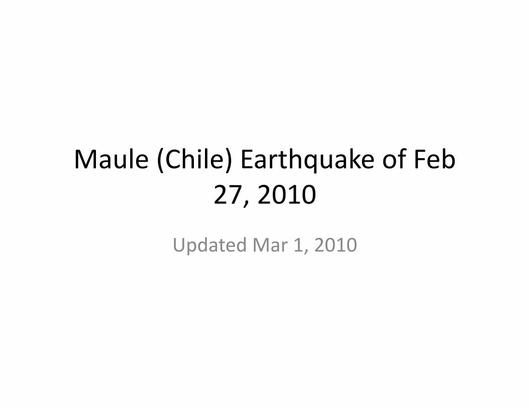
Fig. 5. Elastic modelling of the upper plate deformation in the South Central Chile gap. (a) GPS observations (brown arrows) and model predictions (white arrows) are shown.Inset describes the characteristics of the model. (b) Residual (i.e. observations-model) velocities are shown (black arrow). In both boxes, the grey contour line and shadedpattern draw the subduction plane buried at depth and the white arrows depict the dislocation applied on this plane.

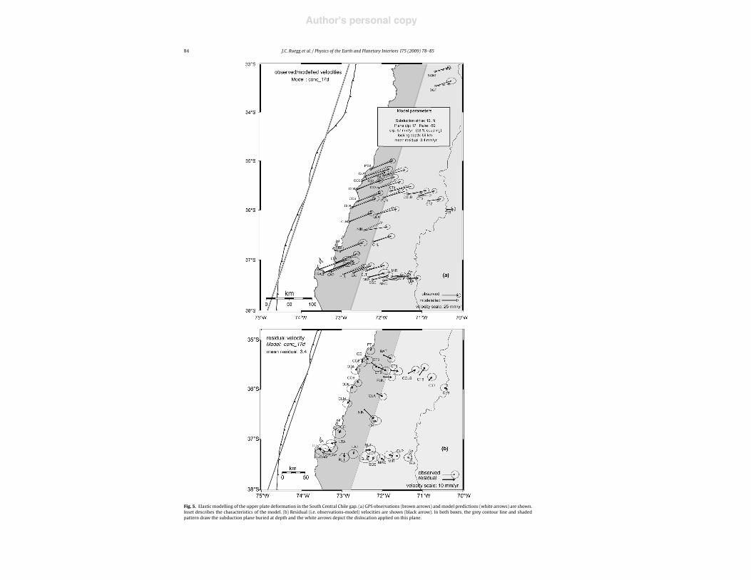
“Finally  a  convergence  moKon  of  about  68mm/year  represents  more  than  10  m  of  displacement  accumulated  since  the  last  big  interplate  subducKon  event  in    this  area  over  170  years  ago  (1835  earthquake  described  by  Darwin).  Therefore,  in  a  worst  case  scenario,  the  area  already  has  a  potenKal  for  an    earthquake  of  magnitude  as  large  as  8–8.5,  should  it  happen  in  the  near  future.”  [Ruegg,  et  al.,  2009]  

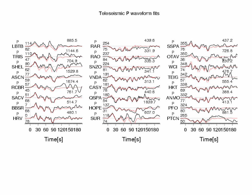
Preliminary  Result  02/27/2010  (Mw  8.8),  Chile  

Anthony  Sladen,  Caltech  

hXp://www.tectonics.caltech.edu/slip_history/2010_chile/index.html  

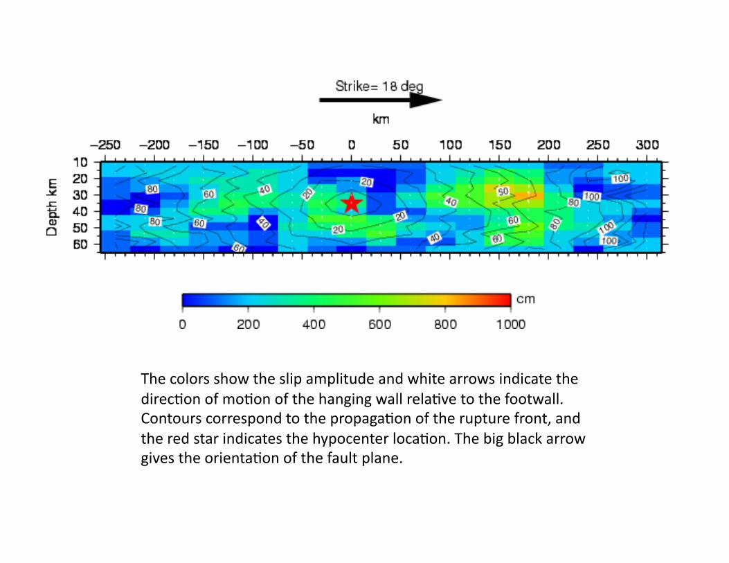
The  colors  show  the  slip  amplitude  and  white  arrows  indicate  the  direcKon  of  moKon  of  the  hanging  wall  relaKve  to  the  footwall.  Contours  correspond  to  the  propagaKon  of  the  rupture  front,  and  the  red  star  indicates  the  hypocenter  locaKon.  The  big  black  arrow  gives  the  orientaKon  of  the  fault  plane.    

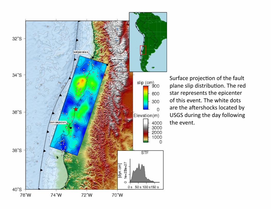
Surface  projecKon  of  the  fault  plane  slip  distribuKon.  The  red  star  represents  the  epicenter  of  this  event.  The  white  dots  are  the  a]ershocks  located  by  USGS  during  the  day  following  the  event.