Embed Size (px)
Citation preview
Gray Matters: Fetal Pollution Exposureand Human Capital Formation
Prashant Bharadwaj, Matthew Gibson, Joshua Graff Zivin, Christopher Neilson
Abstract: This paper examines the impact of fetal exposure to air pollution on fourth-grade test scores in Santiago, Chile. We rely on comparisons across siblings which ad-dress concerns about locational sorting (for nonmovers) and all other time-invariant fam-ily characteristics that can lead to endogenous exposure to poor environmental quality.We also exploit data on air quality alerts to help address concerns related to short-runtime-varying avoidance behavior, which has been shown to be important in a numberof other contexts. We find a strong negative effect from fetal exposure to carbon mon-oxide (CO) and correlated pollutants (like PM10) on math and language skills mea-sured in fourth grade. These effects are economically significant, and our back-of-the-envelope calculations suggest that the 50% reduction in CO in Santiago between 1990and 2005 increased lifetime earnings by approximately US$100 million per birth cohort.
JEL Codes: I24, J24, Q53, Q56
Keywords: Air pollution, Avoidance behavior, Environment and development,Human capital, Sibling comparisons
A LONG LITERATURE in economics has emphasized the important role of humancapital in determining labor market activity and economic growth.1 It is widely be-
Prashant Bharadwaj and Joshua Graff Zivin are at the University of California, San Diego. Mat-thew Gibson ([email protected]) is at Williams College. Christopher Neilson is at PrincetonUniversity. We wish to thank the Departamento de Estasticas e Informacion de Salud del Mi-nisterio de Salud (MINSAL) and Ministry of Education (MINEDUC) of the government ofChile for providing access to the data used in this study.We have also benefited from discussionswith Francisco Gallego, Matthew Neidell, Reed Walker, and participants at PERC Workshopon Environmental Quality and Human Health, NBER Environmental Meetings, University ofSouthern California, University of California, Irvine, Yale University, and the IZA Workshopon Labor Market Effects of Environmental Policies. Financial support from the University ofCalifornia Center for Energy and Environmental Economics is gratefully acknowledged.
1. See Heckman, Lochner, and Todd (2006) for a review on the links between human cap-ital and wages; Romer (1986) and Lucas (1988) form some of the important work showing theimportance of human capital for economic growth.
Received February 10, 2016; Accepted June 03, 2016; Published online April 10, 2017.
JAERE, volume 4, number 2. © 2017 by The Association of Environmental and Resource Economists.All rights reserved. 2333-5955/2017/0402-0005$10.00 http://dx.doi.org/10.1086/691591
505
This content downloaded from 137.110.033.009 on May 01, 2017 11:16:45 AMAll use subject to University of Chicago Press Terms and Conditions (http://www.journals.uchicago.edu/t-and-c).

506 Journal of the Association of Environmental and Resource Economists June 2017
lieved that information technology has increased the private and social returns to ed-ucation, which may partly explain why governments around the world spend an aver-age of 5% of their GDP on education (World Development Indicators 2010) and whyAmericans alone spend more than $7 billion on private tutoring every year (Dizik2013). Yet human capital formation depends on many inputs, and growing literaturesin public health and economics highlight the important role played by prenatal andearly childhood health in this process (Currie and Hyson 1999; Cunha and Heckman2008; Almond and Currie 2011). Pollution has been known to have adverse effects oncontemporaneous childhood health,2 which raises the question of whether early-lifepollution exposure affects long-term human capital outcomes. If so, pollution couldhave a sizable cost to society through its contemporaneous and dynamic effects onthe production of human capital. Such effects may constitute a sizable, and heretoforelargely unmeasured, cost of pollution.
Estimating the relationship between fetal environmental exposures and humancapital outcomes later in life is challenging for two reasons. First, data sets that linkenvironmental and human capital measures over an extended period of time are quiterare. Second, exposure to pollution levels is typically endogenous. Families can engagein both short- and long-run avoidance behaviors to reduce exposure: for example, cur-tailing outdoor activities or moving to a more pristine location. As a result research inthis area has been extremely limited,3 relying on quasi-experimental variation in expo-sure induced by nuclear accidents/testing in data-rich Scandinavian countries (Al-mond, Edlund, and Palme 2009; Black et al. 2013) or policy-induced variation in pol-lution coupled with strong assumptions about individual mobility (Sanders 2012).
In this paper, we employ a unique panel data set from Santiago, Chile, to examinehow fetal exposure to carbon monoxide (and correlated pollutants like PM10 andPM2.5) affects children’s performance on high-stakes national tests in primary school.4
The richness of our data allows us to overcome the core estimation challenges in thisline of research and improve upon the existing literature in several important dimen-sions. First, we can directly link vital statistics and education data through unique in-
2. For recent examples, see Currie and Walker (2011), Knittel, Miller, and Sanders (2011),Arceo-Gomez, Hanna, and Oliva (2012), Currie, Graff Zivin, Meckel, et al. (2013), Currie,Graff Zivin, Mullins, and Neidell (2013), Schlenker and Walker (2015).
3. A notable exception is the literature focused on exposure to lead, a neurotoxin with well-documented impacts on brain development even at modest concentration levels (Sanders et al.2009). Long-term consequences include negative impacts on schooling outcomes, criminal be-havior, and economic productivity (Rogan and Ware 2003; Reyes 2007; Nilsson 2009; Rau,Reyes, and Urzúa 2013).
4. Outcomes in primary school are important to consider as they predict future outcomeslike dropping out of high school (Ensminger and Slusarcick 1992; Garnier, Stein, and Jacobs1997). Research shows that parents are willing to pay more in local school taxes for modest in-creases in test performance in elementary school (Black 1999).
This content downloaded from 137.110.033.009 on May 01, 2017 11:16:45 AMAll use subject to University of Chicago Press Terms and Conditions (http://www.journals.uchicago.edu/t-and-c).

Fetal Pollution Exposure Bharadwaj et al. 507
dividual identifiers. Geographic identifiers allow us to further link to data from pollu-tion monitors operated by the Chilean Ministry of Environment. Moreover our studyperiod, which includes the universe of births between 1992 and 2001, corresponds to aperiod when sustained economic growth and new environmental policy allowed San-tiago to transition from high levels of pollution to more modest ones.
Second, we exploit a multipronged approach to address the endogeneity of pollu-tion exposure. In particular, we rely on sibling comparisons which allow us to addressconcerns about locational sorting (insofar as households do not endogenously movebetween sibling births) and purge estimates of all other time-invariant family charac-teristics, including those that might spuriously influence our core relationship of inter-est in ways that would otherwise be unobservable to the econometrician. As we willdetail below, using sibling fixed effects (FE) yields results that are quite a bit largerthan ordinary least squares (OLS) estimates, suggesting an important role for family-level characteristics.5 We also exploit data on air quality alerts to address short-runtime-varying avoidance behavior, which has proved to be important in a number ofother contexts (Graff Zivin and Neidell 2009; Neidell 2009; Graff Zivin, Neidell,and Schlenker 2011; Deschenes, Greenstone, and Shapiro 2012).
Finally, our paper may shed light on the micro-foundations underpinning the re-cently documented relationship between early-life pollution exposure and labor mar-ket outcomes (Isen, Rossin-Slater, andWalker 2014). It may also help underscore theimplicit trade-offs across economic development paths by highlighting potential feed-back loops between industrialization, human capital formation, and economic growth.The evidence presented in this paper is also of direct policy relevance. Drawing on pre-vious work linking academic achievement and labor productivity, we develop a quan-titative estimate of the social costs of pollution through its effects on human capitalproduction and highlight the sizable benefits accrued from pollution abatement poli-cies implemented during the last two decades. Carbon monoxide is regularly emittedas a by-product of fossil fuel combustion and subject to regulation across the world.6
The human capital impacts from pollution along with any attending avoidance behav-iors constitute additional costs that should be weighed against the relevant benefitsfrom the generation of air pollution.
5. Note that Almond, Edlund, and Palme (2009) also use a sibling FE framework. Sinceendogenous exposure to fallout from the Chernobyl accident in their setting is a minimal con-cern, while exposure was made quite salient to individuals ex post, they interpret their findingsas shedding light on parental investments rather than sorting.
6. It is worth mentioning that an important caveat here is that while we estimate the impactsof carbon monoxide exposure, CO is emitted along with other pollutants and we are unable toseparately identify the impacts of CO versus PM10 versus PM2.5, etc. Later in the paper weshow estimates for these other correlated pollutants as well as a composite index of pollutants(AQI).
This content downloaded from 137.110.033.009 on May 01, 2017 11:16:45 AMAll use subject to University of Chicago Press Terms and Conditions (http://www.journals.uchicago.edu/t-and-c).

508 Journal of the Association of Environmental and Resource Economists June 2017
The remainder of the paper is organized as follows. The next section provides abrief description of the relevant scientific background. Section 2 describes our data,and section 3 details our econometric approach. Our results are described in section 4.Section 5 offers some concluding remarks.
1. SCIENTIFIC BACKGROUND
Carbon monoxide is an odorless and colorless gas that is largely emitted through mo-tor vehicle exhaust (EPA 2008). CO binds to the iron in hemoglobin, inhibiting thebody’s ability to deliver oxygen to vital organs and tissues. The detrimental effects ofCO exposure are magnified in utero. First, the reduced oxygen available to pregnantwomen means less oxygen is delivered to the fetus. Second, carbon monoxide can di-rectly cross the placenta where it more readily binds to fetal hemoglobin (Margulies1986) and remains in the fetal system for an extended period of time (Van Housenet al. 1989). Third, the immature fetal cardiovascular and respiratory systems are par-ticularly sensitive to diminished oxygen levels. Exposure to carbon monoxide in uteroand in early childhood has been linked with lower pulmonary function (Plopper andFanucchi 2000; Neidell 2004; Mortimer et al. 2008). Moreover, most of the damagingeffects of smoking on infant health are believed to be due to the CO contained in cig-arette smoke (World Health Organization 2000).
Animal studies have shown that CO can disrupt critical processes in the developingbrain. The limited evidence suggests that the first and third trimesters of pregnancymay be particularly important. During the first trimester, exposure to CO can impairthe migration of neuroblasts during neurogenesis and thus impede brain development(Woody and Brewster 1990). Exposure to CO during the third trimester can blockimportant receptors that regulate neuronal cell death, leading to neurodegeneration inthe developing rat brain (Ikonomidou et al. 1999). Most directly relevant for our study,a recent epidemiological study of human exposure to wood smoke, of whichCO is amajorconstituent component, found that third-trimester exposure led to long-term deficits inneuropsychological performance (Dix-Cooper et al. 2012). Whether exposure to out-door CO pollution translates into cognitive impairment in humans is largely unknownand the focus of this study.
A common challenge for all nonlaboratory studies of the impacts of air pollution isconfounding due to other pollutants. Some pollutants are co-emitted as a by-productof combustion processes. Others follow opposing seasonal patterns due to heating andcooling patterns and weather more generally. During our study period, Santiago reg-ularly experienced episodes where carbon monoxide, particulate matter (PM), and ozonepollution levels were elevated. While neither PM nor ozone cross the placental barrier,it is still possible that they could damage fetal health through respiratory and cardio-vascular impacts on the mother. A recent study that found CO to be the only pollut-ant to consistently impair infant and child health (Currie, Neidell, and Schmieder
This content downloaded from 137.110.033.009 on May 01, 2017 11:16:45 AMAll use subject to University of Chicago Press Terms and Conditions (http://www.journals.uchicago.edu/t-and-c).

Fetal Pollution Exposure Bharadwaj et al. 509
2009) bolsters the case for our focus on CO but also underscores the importance ofutilizing a multipollutant framework to address potential confounding.
In our setting, environmental confounding could take several distinct forms. InSantiago, like most urban environments, CO exhibits a strong seasonal pattern, withhigh levels in winter and lower levels in summer. Ozone exhibits the opposite pattern,with high levels in summer and lower levels in winter. Thus, if ozone exposure alsoinhibits cognitive formation, ignoring it would lead us to understate the impacts of COpollution.7 To address this, all of our regressions will control for seasonality as well asdirectly control for ozone pollution levels. Ideally, we would include similar controlsfor PM, but given the extremely high correlation between ambient levels of CO andPM in our setting, which typically exceeds 0.9, that is not possible. Rather, we inter-pret our results as the composite effect of CO and PM, recognizing that the epidemi-ological literature points toward CO as the primary culprit in this population.8 Finally,we note that weather, particularly temperature, can impact pollution formation as wellas child health (Deschenes, Greenstone, andGuryan 2009). Thus, we add a wide rangeof controls for weather in order to isolate the deleterious effect of CO. Additional de-tails on these controls can be found in section 3 where we discuss our empirical spec-ification and strategy.
2. DATA
In order to measure the effect of in utero pollution exposure on middle school testscores, we require data from several broad categories. This section describes how weconstruct a data set that links data on births, environmental conditions, and test scores.Our analysis is based on the universe of births in Santiago, Chile, between 1992 and2001 and the corresponding test scores between 2002 and 2010.
2.1. Birth DataBirth data come from a data set (essentially the vital statistics of Chile) provided by theHealth Ministry of the government of Chile. This data set includes information on allthe children born in the years 1992–2001. It provides data on the sex, birth weight,length, and weeks of gestation for each birth. It also provides demographic informa-tion on the parents, including their age, education, marital status, and municipality ofresidence. (Note that a Chilean municipality is a neighborhood, not a city.) Impor-
7. CO and ozone are negatively correlated. Assume for the moment that both pollutantsnegatively affect long-run human capital. If we were to omit the ozone control from our regres-sion, our estimated effect of CO would conflate the harm from high CO with the benefit fromlow ozone. The CO estimate would be biased downward in magnitude.
8. As will be clarified later, our results are largely unchanged when we repeat our core anal-yses using PM rather than CO as our exposure variable.
This content downloaded from 137.110.033.009 on May 01, 2017 11:16:45 AMAll use subject to University of Chicago Press Terms and Conditions (http://www.journals.uchicago.edu/t-and-c).
510 Journal of the Association of Environmental and Resource Economists June 2017
tantly, these data contain a unique code for the mother, allowing us to identify off-spring from the same mother and thus implement sibling fixed effects.
2.2. Environmental DataAir pollution data for the period from 1998 to 2001 come from the Sistema de In-formacion Nacional de Calidad del Aire (SINCA), a network of monitoring stationsoperated by the Chilean Ministry of Environment. Data from 1992–97 come from theMonitoreo Automatica de Contaminantes Atmosfericos Metropolitana (MACAM1)network, also operated by the Ministry.
Given concerns about the endogeneity of monitor “births” and “deaths” (Auff-hammer and Kellogg 2011), our analysis is based on data from the balanced panel ofthree Santiago monitors that operate during our entire study period.9 Two of the mon-itors—Parque O’Higgins and La Independencia—are centrally located and represen-tative of general pollution patterns in metropolitan Santiago (Osses, Gallardo, andFaundez 2013). The third monitor is located in Las Condes, a wealthy suburb in thefoothills of the Andes that sits at high elevation. Pollution patterns at this monitorare quite different since inversion layers, which are correlated with extremely high pol-lution events, occur at altitudes that are lower than this monitor (Gramsch et al. 2006).As a result, we limit our assignment of pollution from the Las Condes monitor to res-idents in the Las Condes municipality. All other residents in Santiago are assigned thepollution readings from the nearest monitor based on municipality centroids.10
CO data during our study period are reported as an 8-hour moving average. Weconstruct a daily average measure of CO from these readings and then compute themean exposure at the trimester level. Data on particulate matter less than 10 micronsin diameter (PM10, measured as a 24-hour moving average) and ozone (O3, measuredhourly) come from the same monitoring sites as our CO data. We follow a similarprocedure to construct mean exposure at the trimester level.
9. In Santiago, new monitor placements arise endogenously from political and bureaucraticprocesses. Use of an unbalanced monitor panel could induce nonzero covariance between expo-sure measurement error and time-varying unobservable determinants of test scores, resulting inbias. Nonetheless we explore this approach in appendix table A2 (appendix and tables A1–A5available online), which shows results using an unbalanced panel of Santiago monitors. Esti-mates are broadly similar, but somewhat smaller in magnitude for math scores. We do not havesimilarly consistent pollution measures for other Chilean cities, e.g., Valparaiso, over this period.
10. Appendix table A3 shows results when we constrain distance to the nearest monitor.Our OLS results are strongest (as expected) when the distance to the nearest monitor is smaller.We have also constructed an alternative exposure measure by taking an inverse-distance weightedaverage over the remaining two monitors for births outside Las Condes. Results are qualitativelysimilar. In addition, assigning all high elevation municipalities (as determined by the mean or me-dian altitude of the municipality) to the Las Condes monitor and using nearest monitor assign-ment among remaining municipalities yields very similar results.
This content downloaded from 137.110.033.009 on May 01, 2017 11:16:45 AMAll use subject to University of Chicago Press Terms and Conditions (http://www.journals.uchicago.edu/t-and-c).

Fetal Pollution Exposure Bharadwaj et al. 511
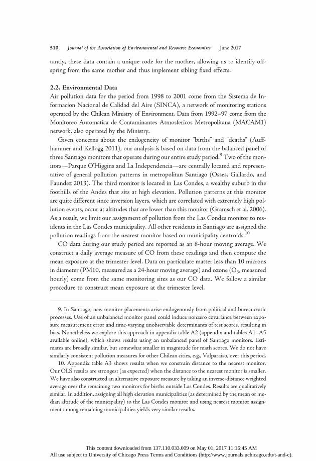
In order to provide a sense of aggregate pollution patterns in Santiago, we use dataon CO, PM10, and O3, to compute a daily Air Quality Index (AQI) using the algo-rithm developed by the US Environmental Protection Agency (EPA 2006; Mintz2012). The AQI is a composite measure of pollution that ranges from 0 to 500 inorder to rank air quality based on its associated health risks. Seasonality in theAQI correlates well with the patterns seen in CO during the year, as is evident fromfigure 1. Air quality is worst during the winter months in Santiago when thermal in-versions are common.
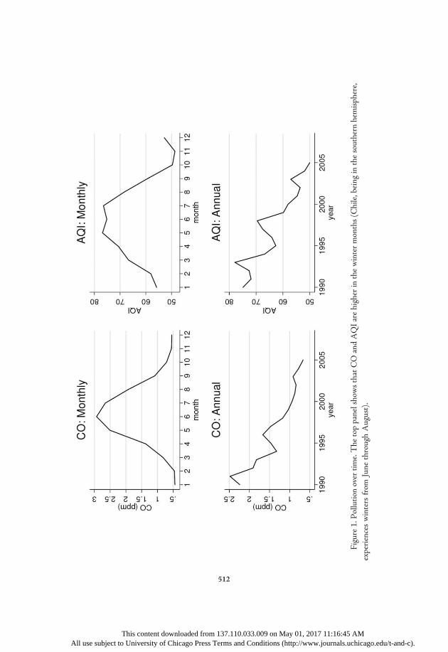
Figure 1 also shows long-run levels of CO and the AQI. As in the seasonal graphs,the two series track each other closely. The steep declines that occur in the mid- tolate-1990s are the result of a concerted government effort to address the serious pol-lution concerns from the previous decade. The most important of these measuresstarted in 1997 under the PPDA (Mullins and Bharadwaj 2014). Figure 2 showsthe monitor-level time series for the three monitors that comprise our balanced panel.They exhibit similar seasonal patterns, but levels are much lower at the Las Condesmonitor than at the Parque O’Higgins and La Independencia monitors.
Meteorological data for this study period come from the NOAA Summary of theDay for the monitor at Comodoro ArturoMerino Benitez International Airport (SCL).Our analysis makes use of daily maximum temperature measures as well as daily av-erage data on rainfall, dew point, wind speed, and an indicator for the presence of fog.Each is converted to a trimester-level measure and used as a nonlinear control in ourregressions, as detailed in section 3.
2.3. Education DataThe data on school achievement are obtained from the SIMCE database, which in-cludes administrative data on test scores for every student in the country between2002 and 2010.11 The SIMCE is a national standardized test administered in allschools in Chile. The SIMCE test covers three main subjects: mathematics, language,and science. It is administered to every student in grade 4, and episodically in grades 8and 10. The SIMCE scores are used to evaluate the progress of students against thenational curriculum goals set out by MINEDUC and are constructed to be compa-rable across schools and time. The education data sets were subsequently matchedto the birth data using individual-level identifiers.12 We are unable to use the eighth-and tenth-grade results in this setting since for these later grades, the number of siblinggroups is far too small: approximately 3,000 for eighth grade and still fewer for tenthgrade.
The match rate between births and SIMCE files (the test score records) is approx-imately 0.8. This match rate, and the fact that Santiago has around 82,500 births per
11. This database was kindly provided by the Ministry of Education of Chile (MINEDUC).12. More details on the match quality can be found in Bharadwaj, Løken, and Neilson 2013.
This content downloaded from 137.110.033.009 on May 01, 2017 11:16:45 AMAll use subject to University of Chicago Press Terms and Conditions (http://www.journals.uchicago.edu/t-and-c).
A
Figure1.Pollutio
novertim
e.The
toppanelshowsthatCO
andAQIarehigherinthewintermonths(Chile,being
inthesouthern
hemisphere,
experienceswintersfrom
June
throughAugust).
512
This content downloaded from 137.110.033.009 on May 01, 2017 11:1ll use subject to University of Chicago Press Terms and Conditions (http://www.journ
6:als
45 A.uc
Mhicago.edu/t-and-c).

A
Figure2.CO
overtim
e,by
monito
r.Eachgraphshow
s90-day
movingaverageCO
(ppm
)atoneof
thethreemonito
rsinourbalanced
panel.
513
This content downloaded from 137.110.033.009 on May 01, 2017 11:16:4ll use subject to University of Chicago Press Terms and Conditions (http://www.journals.
5 Auc
Mhicago.edu/t-and-c).
514 Journal of the Association of Environmental and Resource Economists June 2017
year over our time period, leads to around 66,000 matched observations per year.Over a 10-year period, this is around 660,000 observations. After accounting for ob-servations that are missing essential covariates, we arrive at a potential OLS sample of623,002. Among these observations, the number that have siblings within the agerange observable to us is 193,138. Descriptive statistics for all variables used in ourempirical analysis are presented in table 1.
3. ECONOMETRIC APPROACH
Our goal is to estimate the effect of in utero pollution exposure on human capital out-comes later in life. The primary estimating equation uses test scores as the dependentvariable and pollution exposure in all three trimesters as the independent variables ofinterest. Trimesters are computed using the birth date and the baby’s estimated ges-tational age. The median gestational age in our data is 39 weeks. We assign weeks 1–13 to trimester 1, weeks 14–26 to trimester 2, and weeks 27–birth to trimester 3.13
Since we have the exact date of birth and gestational age, we are able to accuratelyconstruct the history of gestational exposure to ambient air quality. We include all tri-mester exposure measures in a single specification, along with temperature and otherweather variables. Our basic estimating equation is:
Sijrt 5 βEmt 1 vt 1 axijrt 1 gWt 1 εijrt: (1)
The dependent variable Sijrt is fourth-grade test score in either math or language ofchild i, born to mother j, in municipality (neighborhood) r, at time t. The term vt is avector of year and month dummies interacted with three monitor dummies (monthdummies capture important seasonal effects, which differ markedly by monitor),and χ ijrt is a gender dummy. The term Wt includes a host of weather controls (tem-perature, precipitation, fog, dew point, and wind) measured at the trimester level. Weuse a polynomial in the trimester average of precipitation, fog, dew point, and wind inorder to capture potential nonlinear impacts. Since temperature extremes can have adirect effect on maternal behavior and fetal health (Deschenes et al. 2009), and alsoplay a role in pollution formation, we control for temperature more flexibly. In partic-ular, we create 10-degree bins based on daily maximum temperatures and count thenumber of days per trimester in each bin. For example, we include three variables (one pertrimester) counting the number of days with a maximum temperature between 70 and80 degrees Fahrenheit.14
13. While it is easier to interpret and aggregate coefficients at the trimester level, analysis atthe gestational month level yields similar results.
14. Temperature controls are constructed as follows: for each trimester, we count days forwhich maximum temperature falls in each of six 10-degree Fahrenheit bins, 40–49, 50–59, 60–69, 70–79, 80–89, ≥90. This results in 3 trimesters × 6 bins 5 18 count variables.
This content downloaded from 137.110.033.009 on May 01, 2017 11:16:45 AMAll use subject to University of Chicago Press Terms and Conditions (http://www.journals.uchicago.edu/t-and-c).
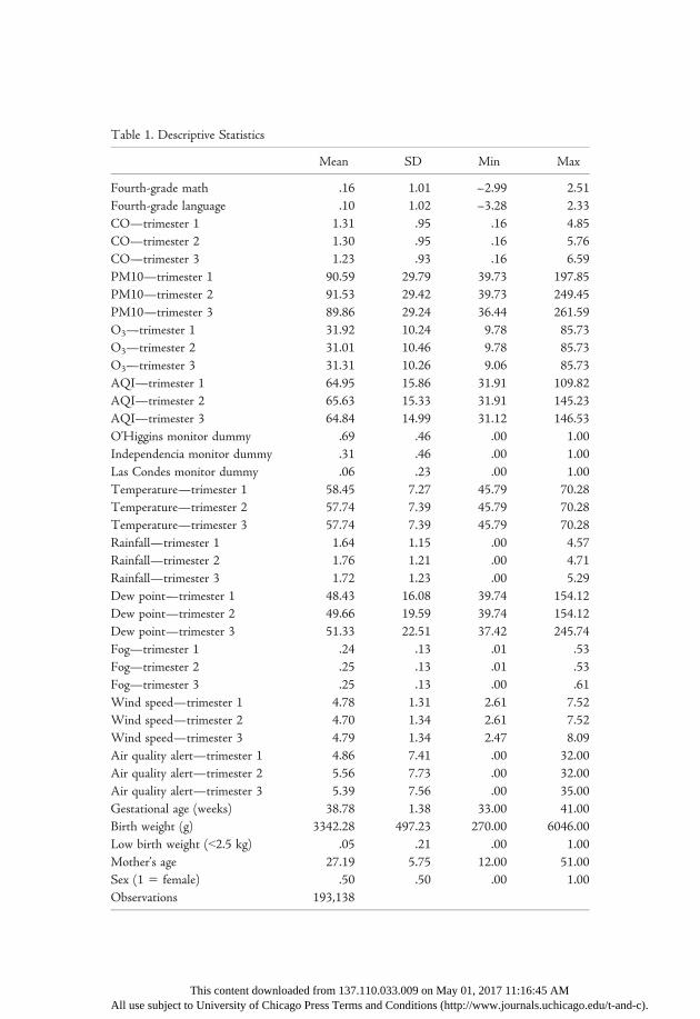
Table 1. Descriptive Statistics
Mean SD Min Max
Fourth-grade math .16 1.01 –2.99 2.51Fourth-grade language .10 1.02 –3.28 2.33CO—trimester 1 1.31 .95 .16 4.85CO—trimester 2 1.30 .95 .16 5.76CO—trimester 3 1.23 .93 .16 6.59PM10—trimester 1 90.59 29.79 39.73 197.85PM10—trimester 2 91.53 29.42 39.73 249.45PM10—trimester 3 89.86 29.24 36.44 261.59O3—trimester 1 31.92 10.24 9.78 85.73O3—trimester 2 31.01 10.46 9.78 85.73O3—trimester 3 31.31 10.26 9.06 85.73AQI—trimester 1 64.95 15.86 31.91 109.82AQI—trimester 2 65.63 15.33 31.91 145.23AQI—trimester 3 64.84 14.99 31.12 146.53O’Higgins monitor dummy .69 .46 .00 1.00Independencia monitor dummy .31 .46 .00 1.00Las Condes monitor dummy .06 .23 .00 1.00Temperature—trimester 1 58.45 7.27 45.79 70.28Temperature—trimester 2 57.74 7.39 45.79 70.28Temperature—trimester 3 57.74 7.39 45.79 70.28Rainfall—trimester 1 1.64 1.15 .00 4.57Rainfall—trimester 2 1.76 1.21 .00 4.71Rainfall—trimester 3 1.72 1.23 .00 5.29Dew point—trimester 1 48.43 16.08 39.74 154.12Dew point—trimester 2 49.66 19.59 39.74 154.12Dew point—trimester 3 51.33 22.51 37.42 245.74Fog—trimester 1 .24 .13 .01 .53Fog—trimester 2 .25 .13 .01 .53Fog—trimester 3 .25 .13 .00 .61Wind speed—trimester 1 4.78 1.31 2.61 7.52Wind speed—trimester 2 4.70 1.34 2.61 7.52Wind speed—trimester 3 4.79 1.34 2.47 8.09Air quality alert—trimester 1 4.86 7.41 .00 32.00Air quality alert—trimester 2 5.56 7.73 .00 32.00Air quality alert—trimester 3 5.39 7.56 .00 35.00Gestational age (weeks) 38.78 1.38 33.00 41.00Birth weight (g) 3342.28 497.23 270.00 6046.00Low birth weight (<2.5 kg) .05 .21 .00 1.00Mother’s age 27.19 5.75 12.00 51.00Sex (1 5 female) .50 .50 .00 1.00Observations 193,138
This content downloadedAll use subject to University of Chicago P
from 137.110.03ress Terms and C
3.009 on May 01onditions (http:/
, 2017 11:16:45/www.journals.u
AMchicago.edu/t-and-c).

516 Journal of the Association of Environmental and Resource Economists June 2017
The term Emt contains the average level of pollution, also measured at the level ofgestational trimester based on the nearest monitor. As discussed in the previous sec-tion, our analysis will focus on the impacts of carbon monoxide on educational out-comes but will also include controls for ozone pollution levels. As a robustness check,we will repeat the same analysis using PM10 as our primary pollutant, with controls forozone levels.15 We will also take a more structured approach to the multipollutantproblem by using the air quality index, which provides a composite measure of environ-mental conditions based on the health dangers associated with CO, PM10, and O3 lev-els (EPA 2006; Mintz 2012).
The seasonal patterns in pollution in Santiago are an important reason behind theinclusion of month and year fixed effects in equation (1). As mentioned earlier, figure 1shows that there are strong monthly patterns to CO and overall air quality as capturedby the AQI. Since these seasonal patterns could exist for other unmeasured variablesthat might impact our outcome of interest (e.g., income-specific timing of childbirth),month fixed effects are an important control in all our specifications. Our approach re-quires residual variation in the measures of pollution after controlling for seasonality(month fixed effects) and year fixed effects. Figure 3 shows the distribution of CO afterremoving these fixed effects; we see that substantial variation remains in the pollutionmeasures. It is this variation that drives the identification in this paper.16
The first modification we make to equation (1) is the introduction of observablemother’s characteristics. Hence, we estimate:
Sijrt 5 βEmt 1 vt 1 axijrt 1 gWt 1 dXj 1 εijrt, (2)
where Xj includes mother’s characteristics like age and education.The identifying assumption in the above equation is that after controlling for ob-
servable maternal characteristics, seasonality and flexible weather controls, exposure topollution is uncorrelated with εijrt. One concern with this assumption is that parentsmay respond to pollution levels, either directly by limiting exposure to pollution orindirectly through ex post investments designed to mitigate harmful effects. Whilesuch responses would not bias our results, they imply that all estimates would capturepollution impacts net of these potentially costly behaviors.17 To clarify the interpre-
15. Recall that the correlation between CO and PM10 levels is 0.9 (see appendix table A1).Also, our results are not sensitive to the use of ozone as a control variable. This is likely due tothe fact that ozone and CO are inversely correlated and seasonal controls do enough to capturethe effects of ozone.
16. Note that while feasible, including year of birth × month of birth fixed effects leaves uswith little residual variation. Results including year × month of birth fixed effects are insignif-icant in the OLS and sibling fixed effects specifications. Results available on request.
17. See Graff Zivin and Neidell (2012) for a detailed conceptual model of the environmen-tal health production function.
This content downloaded from 137.110.033.009 on May 01, 2017 11:16:45 AMAll use subject to University of Chicago Press Terms and Conditions (http://www.journals.uchicago.edu/t-and-c).

Fetal Pollution Exposure Bharadwaj et al. 517
tation of β in our estimation strategy, it is useful to describe a simple education pro-duction function.
We begin by specifying a production function for school achievement, similar inspirit to Todd andWolpin (2007). Test score achievement of student i born to motherj in region r at time t is a function of early childhood health (H),18 investments madefrom birth to time of test taking (P), and parental characteristics (X).
Sijrt 5 f Hijrt, ok5T
k5tPijrk,Xj
!: (3)
Early childhood health is a function of in utero pollution exposure E, weather con-ditions W (e.g., rainfall, temperature, etc.), and parental characteristics X. Individual
Figure 3. Residualized pollution (year and month dummies). Figure based on the residualsof a regression using daily CO as the dependent variable and year and month dummies as inde-pendent variables. We then plot the probability distribution function of the residuals using theStata command “kdensity” with default options: an Epanechnikov kernel and MSE-minimizingbandwidth under an assumed Gaussian distribution.
18. In our specification, t always refers to time of birth, not time of test taking. For the mostpart everyone born at time t takes the test at the same later time (T), since we use scores fromthe national fourth-grade exam.
This content downloaded from 137.110.033.009 on May 01, 2017 11:16:45 AMAll use subject to University of Chicago Press Terms and Conditions (http://www.journals.uchicago.edu/t-and-c).

518 Journal of the Association of Environmental and Resource Economists June 2017
environmental conditions are a function of ambient pollution measured at the nearestmonitor (Emt), mitigated by individual-level avoidance behavior (A).
Hijrt 5 h Eijrt,Wijrt,Xj� �
, (4)
Eijrt 5 e Emt,Aijrt� �
: (5)
Taking a linear approach to estimating equation (3) and plugging in linear func-tions of equations (4) and (5), and recognizing that weather variables are observed citywide, we can express student performance as:
Sijrt 5 βEmt 1 gWt 1 ok5T
k5tnkPijrk 1 hAijrt 1 dXj 1 εijrt: (6)
Equation (1) is essentially a modified version of equation (6). Test scores still de-pend on environmental conditions and parental characteristics and now also dependon time-varying parental investments in human capital as well as pollution avoidancebehaviors during the prenatal period. While educational investments in response toearly-life insults are not observable in our setting (they will be subsumed in our errorterm), studies in other similar contexts have found those responses to be small and ifanything largely compensatory (see Bharadwaj, Eberhard, and Neilson 2013; Hallaand Zweimuller 2014). Thus, to the extent that Chilean parents make investmentsto overcome cognitive deficiencies due to in utero pollution exposure, they will be re-flected in our estimated effects from pollution. This is desirable—it captures the re-alized impacts of pollution—but it is worth noting that the costs of those parental in-vestments may constitute a sizable welfare cost due to pollution.
Avoidance behavior can take two broad forms, and we employ two main techniquesto capture them in our analysis. Since residential sorting can lead to nonrandom assign-ment of pollution, we employ sibling fixed effects models to make within-householdcomparisons that hold geography fixed. This is a particular concern as air quality iscapitalized into housing values (Figueroa, Rogat, and Firinguetti 1996; Chay and Green-stone 2005). Families with higher incomes are more likely to sort into neighborhoodswith better air quality and invest in human capital.19 Sibling fixed effects in this settingalso play an important role insofar as our limited data on maternal characteristics aremissing important unobservable family characteristics that might matter for test out-comes as well as pollution exposure (Currie et al. 2009). Our estimating equation us-
19. Note that our results are robust to the inclusion of municipality (neighborhood) lineartime trends.
This content downloaded from 137.110.033.009 on May 01, 2017 11:16:45 AMAll use subject to University of Chicago Press Terms and Conditions (http://www.journals.uchicago.edu/t-and-c).

Fetal Pollution Exposure Bharadwaj et al. 519
ing sibling fixed effects (indexing another sibling i′ born at t′) is essentially a first dif-ference across siblings and takes the form:
DSijrt–i0 jrt0 5 βDEmt–mt0 1 gDWt–t0 1 Duijrt–i0 jrt0 : (7)
In general the addition of granular fixed effects can exacerbate measurement errorproblems (Griliches and Hausman 1986). In studies of air pollution exposure, how-ever, a spatial error component is often the primary concern. If measurement error isan additively separable function of location, our sibling fixed effects estimates willreduce rather than exacerbate bias from measurement error. In this vein, Jerrettet al. (2005) find that community fixed effects reduce attenuation in estimates of thepollution-mortality relationship. In addition, our sibling fixed effects will capture alltime-invariant investments in children. Equation (7) ignores time-varying investments,however, since we do not have data on parental investments across siblings. One time-varying activity that may influence outcomes is averting behavior. In the short run, in-dividuals can take deliberate actions to reduce their realized exposure to pollution byspending less time outside, wearing face masks, or engaging in a number of other ac-tivities (Neidell 2005, 2009). Such short-run responses require knowledge about dailyor even hourly pollution levels. In our context, that knowledge is made availablethrough a well-publicized system of air quality alerts based on PM10 levels (whichare highly correlated with CO levels). For example, during May–August, the peakpollution months in Santiago, PM10 forecasts are broadcast on a regular basis, withalerts announced when this pollutant reaches certain thresholds (see Mullins andBharadwaj [2014] for details). To the extent that these alerts generate behavioral re-sponses, we can account for them by including controls for the number of alert daysduring the pregnancy for each trimester.20 If individuals engage in avoidance behavior,controlling for avoidance should make the estimates larger relative to estimates wherethis is not explicitly taken into account (Moretti and Neidell 2011). These avoidancecontrols also reduce exposure measurement error arising from differences in indoorand outdoor air quality (Zeger et al. 2000).
We modify equation (7) to take transient avoidance into account as follows:
DSijrt–i0 jrt0 5 βDEmt–mt0 1 gDWt–t0 1 kDAlertst–t0 1 Duijrt–i0 jrt0 : (8)
All of our core analyses will follow the same basic structure. The OLS regression de-scribed in equation (2) will serve as our base model specification. This will be followed
20. Of course, individuals may also engage in avoidance behavior based on the visible signs ofpollution (or its correlates). While we cannot control for those behaviors in this setting, they canbe viewed as conceptually similar to unmeasured parental investments in human capital. Theycreate a wedge between the “biological” and “in situ” impacts of pollution and represent a po-tentially significant welfare cost attributable to pollution.
This content downloaded from 137.110.033.009 on May 01, 2017 11:16:45 AMAll use subject to University of Chicago Press Terms and Conditions (http://www.journals.uchicago.edu/t-and-c).

520 Journal of the Association of Environmental and Resource Economists June 2017
by estimates of the sibling fixed effect regressions described in equation (7). Finally, wewill present estimates of our fully saturated model, which includes sibling fixed effectsand controls for air quality alerts to capture time-varying avoidance behavior, as de-scribed in equation (8).
All
Table 2. CO Effects on Scores
OLS Sib FE Sib FE
A. Math
CO—trimester 1 –.025 –.001 –.000(.017) (.018) (.019)
CO—trimester 2 –.002 –.021 –.022(.011) (.016) (.016)
CO—trimester 3 –.005 –.034** –.036**(.013) (.015) (.016)
CO—whole pregnancy –.032 –.055 –.059*(.027) (.034) (.036)
B. Language
CO—trimester 1 –.040** –.018 –.018(.018) (.017) (.018)
CO—trimester 2 –.017 –.015 –.018(.013) (.015) (.016)
CO—trimester 3 –.025* –.040** –.042**(.014) (.019) (.020)
Sibling FE No Yes YesAir quality alerts No No Yes
Observations 193,138 193,138 193,138CO—whole pregnancy –.082*** –.073** –.078**
(.031) (.037) (.039)
This content downloadeduse subject to University of Chicago P
from 137.110.033.009ress Terms and Condit
on May 01, 2017 11:1ions (http://www.journ
Note. Standard errors are in parentheses, clustered on family andmunicipality (neighborhood).The dependent variable is the fourth-grade math/language SIMCE test score. All regressions in-clude year and month fixed effects interacted with monitor dummies. Demographic controls in-clude student gender, log of mother’s age, and dummies for mother’s education. Environmental con-trols include second-degree polynomials in precipitation, fog, wind speed, and dew point for eachtrimester. Temperature controls are constructed as follows: for each trimester, we count days forwhich maximum temperature falls in each of six 10-degree Fahrenheit bins, 40–49, 50–59, 60–69, 70–79, 80–89, ≥90. This results in 3 trimesters × 6 bins5 18 count variables. We also controlfor ozone pollution (level). All pollution measurements are averaged within each trimester of preg-nancy. We represent an air quality alert with a dummy and sum within each trimester.
* p < .10.** p < .05.*** p < .01.
6:45 AMals.uchicago.edu/t-and-c).

Fetal Pollution Exposure Bharadwaj et al. 521
4. RESULTS
We begin our analysis by examining the impact of CO on test scores in table 2. PanelA presents the estimates using fourth-grade math scores as the dependent variable,and panel B uses fourth-grade language scores as the dependent variable. Column 1is our base OLS specification where we control for seasonality (year and month fixedeffects interacted with monitor dummies), environmental controls at the trimester level(maximum temperature in 10 degree Fahrenheit bin days and a second degree polyno-mial in mean precipitation, fog, wind speed, and dew point), demographic controls(mother’s age and education, student gender), and trimester average ozone levels.21
Standard errors are clustered on family and municipality (neighborhood) in all col-umns. To this base model we add sibling fixed effects in column 2 and further addthe total number of trimester level air quality alert days in column 3. Here and through-out our empirical analysis, we estimate our OLS specification using the sibling sample,facilitating ceterus paribus comparisons across specifications.
Table 2, panel A, shows negative and significant effects of in utero CO exposure onfourth-grade math test scores in specifications that account for sibling fixed effects.22
The effects are concentrated in trimesters 2 and 3 (although estimates for trimester 2are not statistically significant), but taken together, the effect over the entire pregnancyis sizable and statistically significant in our preferred specification. Moving from col-umn 1 to column 2 illustrates the importance of accounting for sorting behavior andother time-invariant unobserved family characteristics in this setting, as the magni-tudes of our estimates increase significantly in column 2. A 1 standard deviation in-crease in CO in the third trimester is initially associated with a statistically insignificant0.005 standard deviation decrease in fourth-grade math scores (col. 1); however, add-ing sibling FE in column 2 increases the magnitude to a statistically significant 0.034standard deviations. Adding air quality alerts to our sibling fixed effects specification(col. 3) increases the magnitude of the estimates slightly (by about 6%–8% in mostcases), suggesting that insofar as the alerts induce avoidance behavior, this appears tohave a rather modest impact on child outcomes.23 Panel B shows similar effects in bothdirection and magnitude on language test scores. The bottom line in each panel presents
21. As discussed in section 1, this study focuses on CO rather than ozone because the sci-entific literature documents the mechanism by which CO harms a developing fetus. Ozone mayalso be harmful to the fetus, but the mechanisms are unknown. Appendix table A4 reports theestimated ozone coefficients from our preferred specification.
22. As described later in this section, our results remain qualitatively similar when we repeatour core analysis replacing CO with PM10 or with AQI.
23. The difference in coefficients from adding the alerts controls is similar for trimesters 2 and3. We caution against overinterpreting this pattern, however. First, these differences are verysmall relative to the associated standard errors. Second, these differences reflect both the quantityof avoidance behavior and its effectiveness, which could vary over the course of a pregnancy.
This content downloaded from 137.110.033.009 on May 01, 2017 11:16:45 AMAll use subject to University of Chicago Press Terms and Conditions (http://www.journals.uchicago.edu/t-and-c).

522 Journal of the Association of Environmental and Resource Economists June 2017
whole-pregnancy effects (sums of trimester-level estimates), which are statistically sig-nificant for language but not for math.
While there are many potential reasons for OLS and sibling fixed effects results tovary in this setting, the fact that OLS seems to underestimate the effect of pollutionexposure is worth noting. This is perhaps counterintuitive if we believe that parentswith worse socioeconomic status live in areas that are more polluted and also have chil-dren who perform worse in school. We offer three potential explanations as to whyOLS might underestimate in this context relative to sibling FE. First, measurementerror (if classical) can bias OLS toward zero. In our case, if measurement error is dif-ferenced out when comparing siblings, then the estimates from sibling FE could belarger than OLS. The second is parental investments. If parents act in ways that tryto compensate for health deficiencies, and parental investments are at least partiallylocal public goods within the household, then we would expect sibling FE estimatesto be larger than OLS. For example, books purchased for one child are likely to benefitothers within the household. In this case, investments that differentially help disad-vantaged children who were exposed to pollution early in life will produce a greater“catch up” compared to children in other households (i.e., OLS) than compared tochildren within the same household (i.e., sibling FE). A full exploration of these forcesis considered in Bharadwaj et al. (2013). The third is avoidance behavior. This is theexplanation used in Moretti and Neidell (2011). In their model, they show that avoid-ance behavior can introduce a downward bias in OLS. The intuition here is simple: ifincreased pollution leads to more avoidance (and more avoidance leads to betterhealth/cognitive scores), then the OLS captures the net effect of exposure and avoid-ance. In strategies that account for avoidance (like the instrumental variables [IV] usedin Moretti and Neidell [2011]), avoidance is held constant, and therefore the IV es-timates are larger than OLS estimates. In our case, sibling fixed effects hold constanttime-invariant avoidance (e.g., fixed cost or lumpy investments or routine patterns ofvariable cost avoidance behaviors) and hence could be yet another explanation as towhy FE estimates are larger than OLS.
Taken as whole, the results in table 2 reveal a strong negative effect from fetal ex-posure to CO.24 While the magnitudes may appear small, it is important to note thattest performance is notoriously difficult to move, even via input-based schooling pol-icies (Hanushek 2003). To place the magnitudes of these effects in context, they areroughly one-fifth the magnitude of successful interventions that specifically target ed-ucational outcomes in developing countries ( JPAL 2014). The economic importanceof these results is underscored by the size of the exposed population—far more chil-
24. An alternative measure is to measure pollution over the entire 9 months of the preg-nancy. This measure yields similar negative and significant effects as seen in the graphs in ap-pendix figures A1 and A2.
This content downloaded from 137.110.033.009 on May 01, 2017 11:16:45 AMAll use subject to University of Chicago Press Terms and Conditions (http://www.journals.uchicago.edu/t-and-c).
Fetal Pollution Exposure Bharadwaj et al. 523
dren are exposed to pollution than well-designed education-specific programs in devel-oping countries. It is also worth noting that our effects are quite a bit larger than es-timates based on changes in total suspended particulates pollution within the UnitedStates (Sanders 2012).25
In table 3, we examine heterogeneity in these human capital impacts by mother’seducation. For both math and language test scores, we see that the effects of CO ex-posure are quite a bit larger for children of mothers without a high school diploma. A1 standard deviation increase in third-trimester CO affects the children of less edu-cated mothers by more than twice as much as the children of more educated mothers(cols. 3 and 6). These results provide suggestive evidence that less educated familiesare more vulnerable to the detrimental effects of pollution. There are several possibleexplanations for this pattern, including but not limited to (1) increased susceptibility,perhaps due to poorer baseline health; (2) increased exposure; and (3) diminished abil-ity to invest in children to offset early-life deficits. Our claims about the vulnerabilityof less educated families are based on evidence that air quality is capitalized into hous-ing prices (Chay and Greenstone 2005; Banzhaf and Walsh 2008). We also note thatGraff Zivin and Neidell (2013) discuss these issues of nonrandom pollution exposuremore generally and provide direct empirical evidence that those households with highersocioeconomic status and higher levels of health investments generally live in neighbor-hoods with better air quality. Conditional on exposure, less educated families may bemore susceptible to pollution due to a range of comorbid conditions, such as asthmaand social stress, which are prevalent among less educated families, and are known toexacerbate the impacts of pollution (e.g., Eggleston et al. 1999; Clougherty et al. 2010).The relative importance of these and other mechanisms remains an open question.
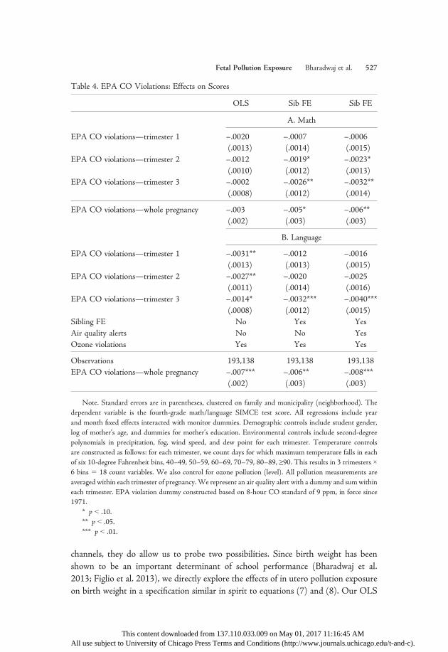
All of our previous analysis treated the relationship between CO exposure and testscores as linear. Figures 4 and 5 show the relationship between pollution and testscores for the third trimester of pregnancy using local linear regressions. The figuresconfirm the negative result found in the previous tables and suggest nonlinearity is notfirst order in this setting. However, we note that there are many ways to model non-linearity in this context. In order to avoid ad hoc searches for nonlinearity, we adoptcounts of violations of the US Environmental Protection Agency’s National AmbientAir Quality Standards for CO (9 parts per million for an 8-hour average)26 as our non-linear exposure measure. To be clear, for each trimester we sum the number of dayson which the EPA’s safety threshold is exceeded. Table 4 presents these results forboth math and language. We find that for every extra day of EPA threshold violation
25. The estimates in Sanders (2012) may be smaller due to measurement error issues. San-ders (2012) infers in utero pollution exposure by assuming that all students were born in theplace they attended high school.
26. The average CO level over a trimester in our sample is approximately 1 part per million.
This content downloaded from 137.110.033.009 on May 01, 2017 11:16:45 AMAll use subject to University of Chicago Press Terms and Conditions (http://www.journals.uchicago.edu/t-and-c).

Table3.
CO
Effectson
Scores,byMother’s
Educatio
n
Math
Math
Math
Language
Language
Language
CO—trimester1
–.014
–.000
.000
–.023
–.010
–.011
(.015)
(.018)
(.019)
(.017)
(.017)
(.018)
CO—trimester2
.003
–.021
–.022
–.011
–.014
–.017
(.012)
(.017)
(.017)
(.014)
(.015)
(.016)
CO—trimester3
–.007
–.025*
–.028*
–.024*
–.030
–.034*
(.012)
(.015)
(.015)
(.014)
(.019)
(.020)
CO—trimester1×lessthan
HS
–.029**
–.004
–.003
–.056***
–.033***
–.028**
(.013)
(.012)
(.012)
(.013)
(.013)
(.012)
CO—trimester2×lessthan
HS
–.028**
.006
.006
–.031**
–.003
–.000
(.013)
(.014)
(.014)
(.013)
(.013)
(.013)
CO—trimester3×lessthan
HS
–.018*
–.041***
–.038***
–.032***
–.045***
–.038***
(.010)
(.010)
(.010)
(.009)
(.011)
(.011)
SiblingFE
No
Yes
Yes
No
Yes
Yes
Airquality
alerts
No
No
Yes
No
No
Yes
Observatio
ns193,138
193,138
193,138
193,138
193,138
193,138
CO—wholepregnancy
–.019
–.046
–.050
–.058**
–.054
–.063
(.024)
(.035)
(.036)
(.029)
(.037)
(.039)
CO—wholepregnancy×lessthan
HS
–.093***
–.085**
–.085**
–.176***
–.134***
–.129***
(.030)
(.035)
(.036)
(.033)
(.038)
(.040)
Note.Standard
errorsareinparentheses,clusteredon
family
andmunicipality
(neighborhood).T
hedependentvariableisthefourth-grade
math/language
SIMCEtestscore.
Allregressionsincludeyear
andmonth
fixedeffectsinteracted
with
monito
rdummies.Dem
ographiccontrolsincludestudentgender,log
ofmother’s
age,anddummiesfor
mother’s
education.
Environmentalcontrolsincludesecond-degreepolynomialsin
precipitatio
n,fog,windspeed,
anddewpointforeach
trimester.Tem
perature
controlsare
constructedas
follows:foreach
trimester,wecountdays
forwhich
maximum
temperature
falls
ineach
ofsix10-degreeFahrenheitbins,40–49,50–59,60–69,70–79,
80–89,≥90.T
hisresultsin3trimesters×6bins
518
countvariables.W
ealso
controlfor
ozonepollutio
n(level).Allpollutio
nmeasurementsareaveraged
with
ineach
trimester
ofpregnancy.W
erepresentan
airquality
alertwith
adummyandsum
with
ineach
trimester.
*p<.10.
**p<.05.
***p<.01.
A
ll use s ubj ect Tto
hisUncoive
ntersit
nt dy o
owf C
nlohic
adago
ed Pr
fromess
1 Te
37.1rms
10.and
033 C
.00ond
9 oitio
n Mns
ay(ht
01tp:/
, 2/ww
017w.
11jou
:16rna
:45ls.u
AMchi
cag o.edu/t-and-c).
Fetal Pollution Exposure Bharadwaj et al. 525
during the third trimester, test scores decrease significantly, with a consistent magni-tude around 0.003 standard deviations using the fixed effects estimates. It is worthnoting that violations of the EPA standard were a regular occurrence in the 1990s inSantiago. For example, in 1997 approximately 47 days exceeded the EPA CO limit,which under linearity would imply an effect of nearly 0.15 standard deviations if all47 violations happened in the second or third trimester. The average number of EPAviolations during a third trimester in our sample is 2.3, which translates to a 0.007 stan-
Figure 4. Residualized math scores and third-trimester CO. The vertical axis measuresresidualized fourth-grade math/language SIMCE test scores. The horizontal axis measuresresidualized third-trimester CO exposure, recentered around mean exposure for ease of inter-pretation. Residualized variables are constructed by regressing these two variables on the full setof controls from our preferred specification, including sibling fixed effects, alerts, and CO expo-sure in trimesters 1–2, then calculating residuals. Other controls include year and month fixedeffects interacted with monitor dummies. Demographic controls include student gender, logof mother’s age, and dummies for mother’s education. Environmental controls include second-degree polynomials in precipitation, fog, wind speed, and dew point. Temperature controlsare constructed as follows: for each trimester, we count days for which maximum temperaturefalls in each of six 10-degree Fahrenheit bins, 40–49, 50–59, 60–69, 70–79, 80–89, ≥90. Thisresults in 3 trimesters × 6 bins5 18 count variables. We also control for ozone pollution (level).All pollution measurements are averaged within each trimester of pregnancy. We represent anair quality alert with a dummy and sum within each trimester. Points represent means within 20equal-frequency bins. Fitted line is a local linear regression over these points, with default kerneland bandwidth. *p < .10; **p < .05; ***p < .01.
This content downloaded from 137.110.033.009 on May 01, 2017 11:16:45 AMAll use subject to University of Chicago Press Terms and Conditions (http://www.journals.uchicago.edu/t-and-c).

526 Journal of the Association of Environmental and Resource Economists June 2017
dard deviation reduction in test scores for the average child exposed to such a thirdtrimester. Appendix table A5 adopts an alternative approach to nonlinearity, allowingCO exposure to enter as counts of third-trimester days in four bins. Consistent withour findings in table 4, there is suggestive evidence that harmful effects stem from themost polluted days, with ambient readings over 3.3 parts per million (ppm).
Thus far our analysis has largely been silent on the various mechanisms that mightunderpin our results. While our data do not allow us to formally disentangle possible
Figure 5. Residualized language scores and third-trimester CO. The vertical axis measuresresidualized fourth-grade math/language SIMCE test scores. The horizontal axis measuresresidualized third-trimester CO exposure, recentered around mean exposure for ease of inter-pretation. Residualized variables are constructed by regressing these two variables on the full setof controls from our preferred specification, including sibling fixed effects, alerts, and CO expo-sure in trimesters 1–2, then calculating residuals. Other controls include year and month fixedeffects interacted with monitor dummies. Demographic controls include student gender, log ofmother’s age, and dummies for mother’s education. Environmental controls include second-degree polynomials in precipitation, fog, wind speed, and dew point. Temperature controls areconstructed as follows: for each trimester, we count days for which maximum temperature fallsin each of six 10-degree Fahrenheit bins, 40–49, 50–59, 60–69, 70–79, 80–89, ≥90. This re-sults in 3 trimesters × 6 bins 5 18 count variables. We also control for ozone pollution (level).All pollution measurements are averaged within each trimester of pregnancy. We represent anair quality alert with a dummy and sum within each trimester. Points represent means within20 equal-frequency bins. Fitted line is a local linear regression over these points, with default ker-nel and bandwidth. *p < .10; **p < .05; ***p < .01.
This content downloaded from 137.110.033.009 on May 01, 2017 11:16:45 AMAll use subject to University of Chicago Press Terms and Conditions (http://www.journals.uchicago.edu/t-and-c).
Fetal Pollution Exposure Bharadwaj et al. 527
channels, they do allow us to probe two possibilities. Since birth weight has beenshown to be an important determinant of school performance (Bharadwaj et al.2013; Figlio et al. 2013), we directly explore the effects of in utero pollution exposureon birth weight in a specification similar in spirit to equations (7) and (8). Our OLS
Table 4. EPA CO Violations: Effects on Scores
OLS Sib FE Sib FE
A. Math
EPA CO violations—trimester 1 –.0020 –.0007 –.0006(.0013) (.0014) (.0015)
EPA CO violations—trimester 2 –.0012 –.0019* –.0023*(.0010) (.0012) (.0013)
EPA CO violations—trimester 3 –.0002 –.0026** –.0032**(.0008) (.0012) (.0014)
EPA CO violations—whole pregnancy –.003 –.005* –.006**(.002) (.003) (.003)
B. Language
EPA CO violations—trimester 1 –.0031** –.0012 –.0016(.0013) (.0013) (.0015)
EPA CO violations—trimester 2 –.0027** –.0020 –.0025(.0011) (.0014) (.0016)
EPA CO violations—trimester 3 –.0014* –.0032*** –.0040***(.0008) (.0012) (.0015)
Sibling FE No Yes YesAir quality alerts No No YesOzone violations Yes Yes Yes
Observations 193,138 193,138 193,138EPA CO violations—whole pregnancy –.007*** –.006** –.008***
(.002) (.003) (.003)
This content downloaded from 13All use subject to University of Chicago Press Term
7.110.033.009 on Ms and Conditions
ay 01, 2017 11:16:(http://www.journal
Note. Standard errors are in parentheses, clustered on family and municipality (neighborhood). Thedependent variable is the fourth-grade math/language SIMCE test score. All regressions include yearand month fixed effects interacted with monitor dummies. Demographic controls include student gender,log of mother’s age, and dummies for mother’s education. Environmental controls include second-degreepolynomials in precipitation, fog, wind speed, and dew point for each trimester. Temperature controlsare constructed as follows: for each trimester, we count days for which maximum temperature falls in eachof six 10-degree Fahrenheit bins, 40–49, 50–59, 60–69, 70–79, 80–89, ≥90. This results in 3 trimesters ×6 bins 5 18 count variables. We also control for ozone pollution (level). All pollution measurements areaveraged within each trimester of pregnancy.We represent an air quality alert with a dummy and sumwithineach trimester. EPA violation dummy constructed based on 8-hour CO standard of 9 ppm, in force since1971.
* p < .10.** p < .05.*** p < .01.
45 AMs.uchicago.edu/t-and-c).
528 Journal of the Association of Environmental and Resource Economists June 2017
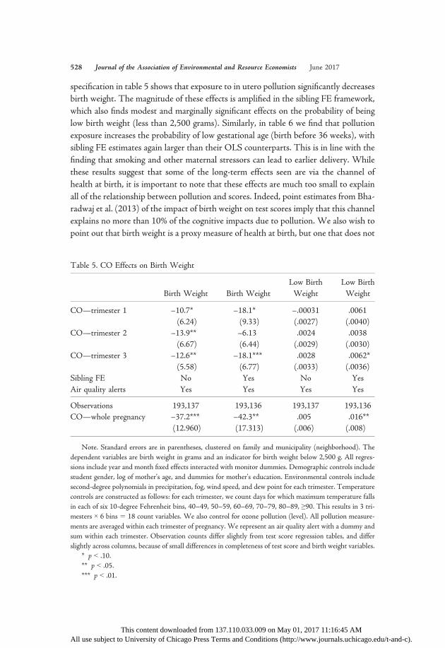
specification in table 5 shows that exposure to in utero pollution significantly decreasesbirth weight. The magnitude of these effects is amplified in the sibling FE framework,which also finds modest and marginally significant effects on the probability of beinglow birth weight (less than 2,500 grams). Similarly, in table 6 we find that pollutionexposure increases the probability of low gestational age (birth before 36 weeks), withsibling FE estimates again larger than their OLS counterparts. This is in line with thefinding that smoking and other maternal stressors can lead to earlier delivery. Whilethese results suggest that some of the long-term effects seen are via the channel ofhealth at birth, it is important to note that these effects are much too small to explainall of the relationship between pollution and scores. Indeed, point estimates from Bha-radwaj et al. (2013) of the impact of birth weight on test scores imply that this channelexplains no more than 10% of the cognitive impacts due to pollution. We also wish topoint out that birth weight is a proxy measure of health at birth, but one that does not
Table 5. CO Effects on Birth Weight
Birth Weight Birth WeightLow BirthWeight
Low BirthWeight
CO—trimester 1 –10.7* –18.1* –.00031 .0061(6.24) (9.33) (.0027) (.0040)
CO—trimester 2 –13.9** –6.13 .0024 .0038(6.67) (6.44) (.0029) (.0030)
CO—trimester 3 –12.6** –18.1*** .0028 .0062*(5.58) (6.77) (.0033) (.0036)
Sibling FE No Yes No YesAir quality alerts Yes Yes Yes Yes
Observations 193,137 193,136 193,137 193,136CO—whole pregnancy –37.2*** –42.3** .005 .016**
(12.960) (17.313) (.006) (.008)
This content dAll use subject to University o
ownloaded from 137f Chicago Press Term
.110.033.009 on Mas and Conditions (ht
y 01, 2017 11:16:tp://www.journal
Note. Standard errors are in parentheses, clustered on family and municipality (neighborhood). Thedependent variables are birth weight in grams and an indicator for birth weight below 2,500 g. All regres-sions include year and month fixed effects interacted with monitor dummies. Demographic controls includestudent gender, log of mother’s age, and dummies for mother’s education. Environmental controls includesecond-degree polynomials in precipitation, fog, wind speed, and dew point for each trimester. Temperaturecontrols are constructed as follows: for each trimester, we count days for which maximum temperature fallsin each of six 10-degree Fehrenheit bins, 40–49, 50–59, 60–69, 70–79, 80–89, ≥90. This results in 3 tri-mesters × 6 bins 5 18 count variables. We also control for ozone pollution (level). All pollution measure-ments are averaged within each trimester of pregnancy. We represent an air quality alert with a dummy andsum within each trimester. Observation counts differ slightly from test score regression tables, and differslightly across columns, because of small differences in completeness of test score and birth weight variables.
* p < .10.** p < .05.*** p < .01.
45 AMs.uchicago.edu/t-and-c).

Fetal Pollution Exposure Bharadwaj et al. 529
capture all aspects of fetal health or nutrition (Almond and Currie 2011). Moreover,maternal health stressors, such as pollution, can directly impact gene expression in thefetus through epigenetic channels that negatively impact intellectual growth and ma-turity (Petronis 2010).
4.1. Robustness ChecksAs mentioned earlier, due to the high correlation between CO and PM10, our mainspecifications do not control for PM10. Hence, replacing CO with PM10 should yieldqualitatively similar results. In table 7, we find that this is indeed the case. Across allthree of our specifications, we find that exposure to PM10 in utero is associated withsignificant negative effects on fourth-grade math and language scores. An alternativeapproach to addressing multiple pollutants is to aggregate them into a single index. Inthis case, we use the US Environmental Protection Agency’s Air Quality Index (AQI),which is constructed by taking the maximum over piecewise-linear transformations
All use
Table 6. CO Effects on Low Gestational Age
Low GA Low GA Low GA
CO—trimester 1 .0078*** .010*** .010***(.0028) (.0027) (.0030)
CO—trimester 2 .014*** .0081** .0049(.0033) (.0032) (.0035)
CO—trimester 3 .010*** .0092*** .0059**(.0030) (.0027) (.0029)
Sibling FE No Yes YesAir quality alerts No No Yes
Observations 193,138 193,138 193,138CO—whole pregnancy .032*** .028*** .021***
(.007) (.006) (.007)
This content downloaded subject to University of Chicago P
from 137.110.033.0ress Terms and Cond
09 on May 01, 2017 itions (http://www.j
Note. Standard errors are in parentheses, clustered on family and municipality (neigh-borhood). The dependent variable is an indicator for gestational age below 36 weeks. Allregressions include year and month fixed effects interacted with monitor dummies. Demo-graphic controls include student gender, log of mother’s age, and dummies for mother’s ed-ucation. Environmental controls include second-degree polynomials in precipitation, fog,wind speed, and dew point for each trimester. Temperature controls are constructed as fol-lows: for each trimester, we count days for which maximum temperature falls in each ofsix 10-degree Fahrenheit bins, 40–49, 50–59, 60–69, 70–79, 80–89, ≥90. This resultsin 3 trimesters × 6 bins 5 18 count variables. We also control for ozone pollution (level).All pollution measurements are averaged within each trimester of pregnancy. We representan air quality alert with a dummy and sum within each trimester.
* p < .10.** p < .05.*** p < .01.
11:16:45 AMournals.uchicago.edu/t-and-c).

530 Journal of the Association of Environmental and Resource Economists June 2017
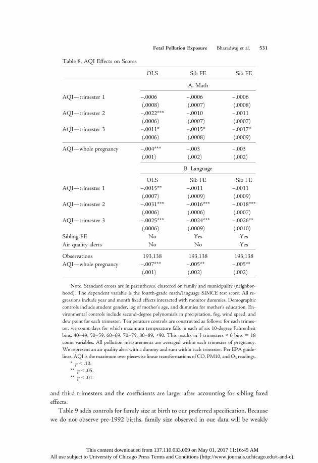
of daily readings for all individual pollutants (EPA 2006; Mintz 2012). As can be seenin table 8, higher AQI exposure in utero leads to lower test scores. While this approachdoes not allow us to disentangle the effects of different pollutants, these results followthe same patterns as prior tables—most of the effects are concentrated in the second
All us
Table 7. PM10 Effects on Scores
OLS Sib FE Sib FE
A. Math
PM10—trimester 1 –.0004 –.0002 –.0001(.0005) (.0005) (.0006)
PM10—trimester 2 –.0006 –.0003 –.0003(.0004) (.0005) (.0005)
PM10—trimester 3 –.0009* –.0010* –.0011*(.0005) (.0005) (.0006)
PM10—whole pregnancy –.002 –.001 –.001(.001) (.001) (.001)
B. Language
PM10—trimester 1 –.0010** –.0008 –.0008(.0005) (.0005) (.0005)
PM10—trimester 2 –.0011** –.0006 –.0006(.0005) (.0004) (.0004)
PM10—trimester 3 –.0013*** –.0013** –.0013**(.0004) (.0006) (.0006)
Sibling FE No Yes YesAir quality alerts No No Yes
Observations 193,138 193,138 193,138PM10—whole pregnancy –.003*** –.003*** –.003***
(.001) (.001) (.001)
This content downloaded fe subject to University of Chicago Pre
rom 137.110.033.009ss Terms and Condit
on May 01, 2017 1ions (http://www.jo
Note. Standard errors are in parentheses, clustered on family and municipality (neighbor-hood). The dependent variable is the fourth-grade math/language SIMCE test score. All re-gressions include year and month fixed effects interacted with monitor dummies. Demographiccontrols include student gender, log of mother’s age, and dummies for mother’s education. En-vironmental controls include second-degree polynomials in precipitation, fog, wind speed, anddew point for each trimester. Temperature controls are constructed as follows: for each tri-mester, we count days for which maximum temperature falls in each of six 10-degree Fahren-heit bins, 40–49, 50–59, 60–69, 70–79, 80–89, ≥90. This results in 3 trimesters × 6 bins 518 count variables. We also control for ozone pollution (level). All pollution measurementsare averaged within each trimester of pregnancy.We represent an air quality alert with a dummyand sum within each trimester.
* p < .10.** p < .05.*** p < .01.
1:16:45 AMurnals.uchicago.edu/t-and-c).
Fetal Pollution Exposure Bharadwaj et al. 531
and third trimesters and the coefficients are larger after accounting for sibling fixedeffects.
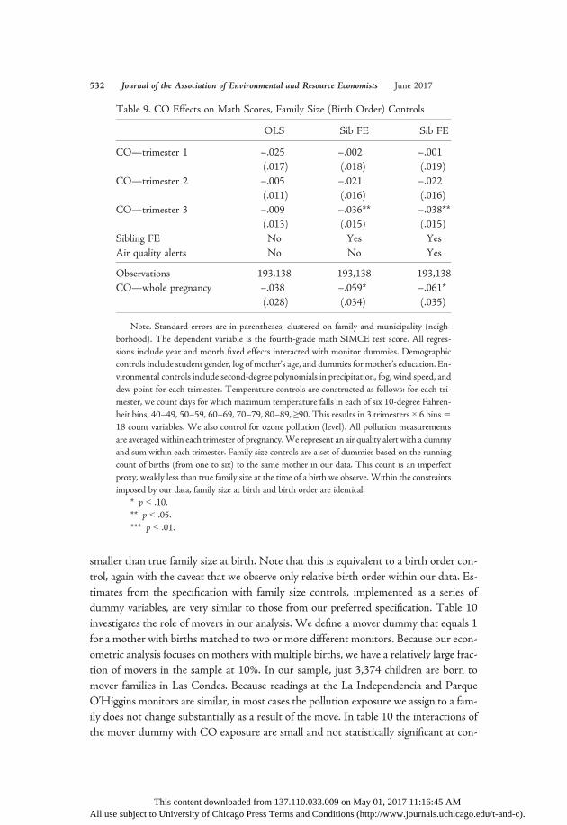
Table 9 adds controls for family size at birth to our preferred specification. Becausewe do not observe pre-1992 births, family size observed in our data will be weakly
All u
Table 8. AQI Effects on Scores
OLS Sib FE Sib FE
A. Math
AQI—trimester 1 –.0006 –.0006 –.0006(.0008) (.0007) (.0008)
AQI—trimester 2 –.0022*** –.0010 –.0011(.0006) (.0007) (.0007)
AQI—trimester 3 –.0011* –.0015* –.0017*(.0006) (.0008) (.0009)
AQI—whole pregnancy –.004*** –.003 –.003(.001) (.002) (.002)
B. Language
OLS Sib FE Sib FEAQI—trimester 1 –.0015** –.0011 –.0011
(.0007) (.0009) (.0009)AQI—trimester 2 –.0031*** –.0016*** –.0018***
(.0006) (.0006) (.0007)AQI—trimester 3 –.0025*** –.0024*** –.0026**
(.0006) (.0009) (.0010)Sibling FE No Yes YesAir quality alerts No No Yes
Observations 193,138 193,138 193,138AQI—whole pregnancy –.007*** –.005** –.005**
(.001) (.002) (.002)
This content downloadedse subject to University of Chicago P
from 137.110.033.0ress Terms and Cond
09 on May 01, 2017 1itions (http://www.jo
Note. Standard errors are in parentheses, clustered on family and municipality (neighbor-hood). The dependent variable is the fourth-grade math/language SIMCE test score. All re-gressions include year and month fixed effects interacted with monitor dummies. Demographiccontrols include student gender, log of mother’s age, and dummies for mother’s education. En-vironmental controls include second-degree polynomials in precipitation, fog, wind speed, anddew point for each trimester. Temperature controls are constructed as follows: for each trimes-ter, we count days for which maximum temperature falls in each of six 10-degree Fahrenheitbins, 40–49, 50–59, 60–69, 70–79, 80–89, ≥90. This results in 3 trimesters × 6 bins 5 18count variables. All pollution measurements are averaged within each trimester of pregnancy.We represent an air quality alert with a dummy and sum within each trimester. Per EPA guide-lines, AQI is the maximum over piecewise linear transformations of CO, PM10, andO3 readings.
* p < .10.** p < .05.** p < .01.
1:16:45 AMurnals.uchicago.edu/t-and-c).
532 Journal of the Association of Environmental and Resource Economists June 2017
smaller than true family size at birth. Note that this is equivalent to a birth order con-trol, again with the caveat that we observe only relative birth order within our data. Es-timates from the specification with family size controls, implemented as a series ofdummy variables, are very similar to those from our preferred specification. Table 10investigates the role of movers in our analysis. We define a mover dummy that equals 1for a mother with births matched to two or more different monitors. Because our econ-ometric analysis focuses on mothers with multiple births, we have a relatively large frac-tion of movers in the sample at 10%. In our sample, just 3,374 children are born tomover families in Las Condes. Because readings at the La Independencia and ParqueO’Higgins monitors are similar, in most cases the pollution exposure we assign to a fam-ily does not change substantially as a result of the move. In table 10 the interactions ofthe mover dummy with CO exposure are small and not statistically significant at con-
All us
Table 9. CO Effects on Math Scores, Family Size (Birth Order) Controls
OLS Sib FE Sib FE
CO—trimester 1 –.025 –.002 –.001(.017) (.018) (.019)
CO—trimester 2 –.005 –.021 –.022(.011) (.016) (.016)
CO—trimester 3 –.009 –.036** –.038**(.013) (.015) (.015)
Sibling FE No Yes YesAir quality alerts No No Yes
Observations 193,138 193,138 193,138CO—whole pregnancy –.038 –.059* –.061*
(.028) (.034) (.035)
This content downloaded fe subject to University of Chicago Pr
rom 137.110.033.00ess Terms and Condi
9 on May 01, 2017 11tions (http://www.jou
Note. Standard errors are in parentheses, clustered on family and municipality (neigh-borhood). The dependent variable is the fourth-grade math SIMCE test score. All regres-sions include year and month fixed effects interacted with monitor dummies. Demographiccontrols include student gender, log of mother’s age, and dummies for mother’s education. En-vironmental controls include second-degree polynomials in precipitation, fog, wind speed, anddew point for each trimester. Temperature controls are constructed as follows: for each tri-mester, we count days for which maximum temperature falls in each of six 10-degree Fahren-heit bins, 40–49, 50–59, 60–69, 70–79, 80–89, ≥90. This results in 3 trimesters × 6 bins518 count variables. We also control for ozone pollution (level). All pollution measurementsare averaged within each trimester of pregnancy.We represent an air quality alert with a dummyand sum within each trimester. Family size controls are a set of dummies based on the runningcount of births (from one to six) to the same mother in our data. This count is an imperfectproxy, weakly less than true family size at the time of a birth we observe. Within the constraintsimposed by our data, family size at birth and birth order are identical.
* p < .10.** p < .05.*** p < .01.
:16:45 AMrnals.uchicago.edu/t-and-c).

Fetal Pollution Exposure Bharadwaj et al. 533
ventional levels. The sums of exposure coefficients for movers and nonmovers are nearlyidentical. This suggests that moves do not create a correlation between our CO expo-sure measures and time-varying unobservable determinants of test scores.
Table 11 shows that CO exposure in trimesters prior to conception does not play arole in determining test scores. This is important and reassuring, as it shows that our
All use s
Table 10. CO Effects on Math Scores, Interacted with Moving
OLS Sib FE Sib FE
CO—trimester 1 –.029 –.000 .001(.019) (.018) (.019)
CO—trimester 2 –.001 –.020 –.021(.011) (.016) (.016)
CO—trimester 3 –.007 –.035** –.037**(.013) (.015) (.015)
CO—trimester 1 × mover .053* –.010 –.010(.027) (.014) (.014)
CO—trimester 2 × mover –.000 –.008 –.008(.016) (.017) (.017)
CO—trimester 3 × mover .041* .018 .018(.022) (.012) (.012)
Sibling FE No Yes YesAir quality alerts No No Yes
Observations 193,138 193,138 193,138CO—whole pregnancy –.037 –.055 –.058
(.027) (.034) (.036)CO—whole pregnancy, mover .056 –.054 –.057
(.041) (.038) (.039)
This content downloaded from 1ubject to University of Chicago Press Te
37.110.033.009 rms and Conditio
on May 01, 2017ns (http://www.
Note. Standard errors are in parentheses, clustered on family and municipality(neighborhood). The dependent variable is the fourth-grade math SIMCE test score.All regressions include year and month fixed effects interacted with monitor dummies.Demographic controls include student gender, log of mother’s age, and dummies formother’s education. Environmental controls include second-degree polynomials in pre-cipitation, fog, wind speed, and dew point for each trimester. Temperature controls areconstructed as follows: for each trimester, we count days for which maximum tempera-ture falls in each of six 10-degree Fahrenheit bins, 40–49, 50–59, 60–69, 70–79, 80–89,≥90. This results in 3 trimesters × 6 bins5 18 count variables.We also control for ozonepollution (level). All pollution measurements are averaged within each trimester of preg-nancy. We represent an air quality alert with a dummy and sum within each trimester.The movers dummy equals 1 for mothers matched to two or more pollution monitors.
* p < .10.** p < .05.*** p < .01.
11:16:45 AMjournals.uchicago.edu/t-and-c).
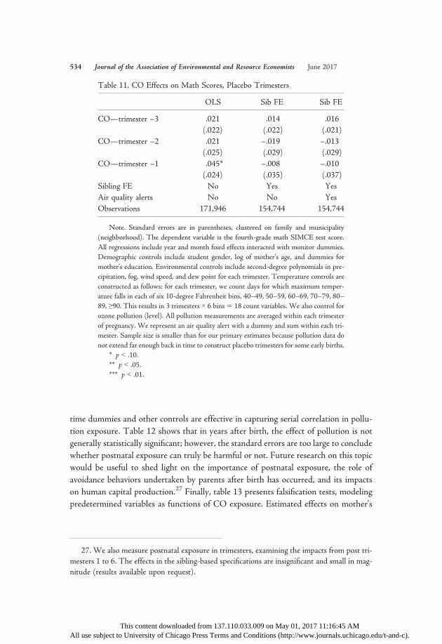
534 Journal of the Association of Environmental and Resource Economists June 2017
time dummies and other controls are effective in capturing serial correlation in pollu-tion exposure. Table 12 shows that in years after birth, the effect of pollution is notgenerally statistically significant; however, the standard errors are too large to concludewhether postnatal exposure can truly be harmful or not. Future research on this topicwould be useful to shed light on the importance of postnatal exposure, the role ofavoidance behaviors undertaken by parents after birth has occurred, and its impactson human capital production.27 Finally, table 13 presents falsification tests, modelingpredetermined variables as functions of CO exposure. Estimated effects on mother’s
27. Wmestersnitude (
All use s
Table 11. CO Effects on Math Scores, Placebo Trimesters
OLS Sib FE Sib FE
CO—trimester –3 .021 .014 .016(.022) (.022) (.021)
CO—trimester –2 .021 –.019 –.013(.025) (.029) (.029)
CO—trimester –1 .045* –.008 –.010(.024) (.035) (.037)
Sibling FE No Yes YesAir quality alerts No No YesObservations 171,946 154,744 154,744
e also measure postnatal expos1 to 6. The effects in the siblingresults available upon request).
This content downloaded ubject to University of Chicago Pr
ure in trimesters, e-based specification
from 137.110.033.0ess Terms and Con
xamining the impas are insignificant
09 on May 01, 2017ditions (http://www.
Note. Standard errors are in parentheses, clustered on family and municipality(neighborhood). The dependent variable is the fourth-grade math SIMCE test score.All regressions include year and month fixed effects interacted with monitor dummies.Demographic controls include student gender, log of mother’s age, and dummies formother’s education. Environmental controls include second-degree polynomials in pre-cipitation, fog, wind speed, and dew point for each trimester. Temperature controls areconstructed as follows: for each trimester, we count days for which maximum temper-ature falls in each of six 10-degree Fahrenheit bins, 40–49, 50–59, 60–69, 70–79, 80–89, ≥90. This results in 3 trimesters × 6 bins5 18 count variables. We also control forozone pollution (level). All pollution measurements are averaged within each trimesterof pregnancy. We represent an air quality alert with a dummy and sum within each tri-mester. Sample size is smaller than for our primary estimates because pollution data donot extend far enough back in time to construct placebo trimesters for some early births.
* p < .10.** p < .05.*** p < .01.
cts from post tri-and small in mag-
11:16:45 AMjournals.uchicago.edu/t-and-c).

Fetal Pollution Exposure Bharadwaj et al. 535
age, father’s age, and mother’s education are near zero and statistically insignificant,revealing no evidence of bias from gross misspecification.
5. CONCLUSION
In this paper, we merge data from the Chilean ministries of health and education withpollution and meteorological data to assess the impact of fetal air pollution exposureon human capital outcomes later in life. Data on air quality alerts and the use of sib-ling fixed effects estimation allow us to address several potentially important concernsabout endogenous exposure to poor environmental quality. We find a strong and ro-bust negative effect from fetal exposure to CO on math and language skills. Our re-sults are also in line with the scientific literature suggesting the importance of the firstand third trimesters in fetal brain development. Our richest model specification sug-gests that a 1 standard deviation increase in CO exposure during the third trimester of
All use s
Table 12. CO Effects on Math Scores, Postnatal Years
OLS Sib FE Sib FE
CO—year 1 .032 .007 .008(.034) (.042) (.043)
CO—year 2 .040 .094** .087**(.045) (.044) (.044)
CO—year 3 –.091 –.048 –.055(.060) (.069) (.068)
CO—year 4 .061 .038 .026(.159) (.142) (.142)
Sibling FE No Yes YesAir quality alerts No No YesObservations 193,138 193,138 193,138
This content downloubject to University of Chic
aded from 137.110.03ago Press Terms and C
3.009 on May 01, 2017onditions (http://www.
Note. Standard errors are in parentheses, clustered on family and municipality(neighborhood). The dependent variable is the fourth-grade math SIMCE test score.All regressions include year and month fixed effects interacted with monitor dummies.Demographic controls include student gender, log of mother’s age, and dummies formother’s education. Environmental controls include second-degree polynomials in pre-cipitation, fog, wind speed, and dew point for each trimester or year. Temperature con-trols are constructed as follows: for each trimester or year, we count days for which max-imum temperature falls in each of six 10-degree Fahrenheit bins, 40–49, 50–59, 60–69,70–79, 80–89, ≥90. This results in (3 trimesters × 6 bins) 1 (4 years × 6 bins) 5 42count variables. We also control for ozone pollution (level). All pollution measurementsare averaged within each trimester or year of pregnancy. We represent an air qualityalert with a dummy and sum within each trimester or year.
* p < .10.** p < .05.*** p < .01.
11:16:45 AMjournals.uchicago.edu/t-and-c).
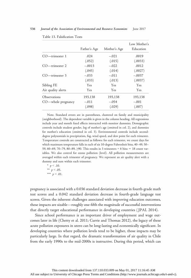
536 Journal of the Association of Environmental and Resource Economists June 2017
pregnancy is associated with a 0.036 standard deviation decrease in fourth-grade mathtest scores and a 0.042 standard deviation decrease in fourth-grade language testscores. Given the inherent challenges associated with improving education outcomes,these impacts are sizable—roughly one-fifth the magnitude of successful interventionsthat directly target educational performance in developing countries ( JPAL 2014).
Since school performance is an important driver of employment and wage out-comes later in life (Chetty et al. 2011; Currie and Thomas 2012), the legacy of theseacute pollution exposures in utero can be long-lasting and economically significant. Indeveloping countries where pollution levels tend to be higher, those impacts may beparticularly large. In that regard, the dramatic transformation of air quality in Chilefrom the early 1990s to the mid-2000s is instructive. During this period, which can
All use s
Table 13. Falsification Tests
Father’s Age Mother’s AgeLow Mother’sEducation
CO—trimester 1 .024 –.021 .0019(.052) (.015) (.0033)
CO—trimester 2 –.0013 –.022 .0012(.045) (.014) (.0027)
CO—trimester 3 –.033 –.011 –.0037(.033) (.013) (.0037)
Sibling FE Yes Yes YesAir quality alerts Yes Yes Yes
Observations 193,138 193,138 193,138CO—whole pregnancy –.011 –.054 –.001
(.098) (.029) (.007)
This content downloaubject to University of Chicag
ded from 137.110o Press Terms and
.033.009 on May 01 Conditions (http:/
Note. Standard errors are in parentheses, clustered on family and municipality(neighborhood). The dependent variable is given in the column heading. All regressionsinclude year and month fixed effects interacted with monitor dummies. Demographiccontrols include student gender, log of mother’s age (omitted in col. 2), and dummiesfor mother’s education (omitted in col. 3). Environmental controls include second-degree polynomials in precipitation, fog, wind speed, and dew point for each trimester.Temperature controls are constructed as follows: for each trimester, we count days forwhich maximum temperature falls in each of six 10-degree Fahrenheit bins, 40–49, 50–59, 60–69, 70–79, 80–89, ≥90. This results in 3 trimesters × 6 bins 5 18 count var-iables. We also control for ozone pollution (level). All pollution measurements areaveraged within each trimester of pregnancy. We represent an air quality alert with adummy and sum within each trimester.
* p < .10.** p < .05.*** p < .01.
, 2017 11:16:45 AM/www.journals.uchicago.edu/t-and-c).
Fetal Pollution Exposure Bharadwaj et al. 537
be viewed as a transition from typical developing country urban pollution levels to lev-els that are closer to those found in typical developed country cities, average CO levelsin Santiago dropped by more than 50%. A back-of-the-envelope calculation using ourestimated human capital effects and estimates on the returns to test scores from theUnited States (Blau and Kahn 2005) suggests that, ceteris paribus, this drop couldaccount for as much as $1,000 in additional lifetime earnings per child born under thecleaner regime. During our sample period on average 100,000 children are born everyyear in Santiago, suggesting a lifetime increase of US$100 million per cohort.28 It isimportant to realize that most of the costs of pollution exposure might be borne by theless fortunate. Such results may help explain patterns of wealth accumulation around theworld, where the poor tend to live in neighborhoods with low environmental quality,which diminishes cognitive attainment and thus limits opportunities to rise out of pov-erty. The sizable nonpecuniary benefits from education (Oreopoulos and Salvanes2011) only serve to magnify these welfare impacts.
Our empirical results are also of direct importance for policy makers. Carbon mon-oxide is directly regulated throughout the developed and an increasing share of thedeveloping world. Nearly all of these regulations are based on the benefits associatedwith reductions in pollution-related health problems, mortality, and hospitaliza-tions.29 Our results suggest that such an approach underestimates regulatory benefitsfor at least two reasons. First, it completely ignores the human capital effects, whichhave been largely invisible but may well rival the more dramatic health effects in mag-nitude since they affect a much broader swath of the population. Second, it fails toaccount for the costs of short- and long-run avoidance behaviors for which we findevidence. While our empirical framework does not allow us to assess the magnitudeof these costs, they have been found to be substantial in other settings (Graff Zivin
28. This number is calculated as follows. The change in average CO levels between 1992 and2002 is equivalent to a 1 standard deviation change in CO pollution levels. Using our sibling FEresults for math performance in the third trimester (this is conservative, as the improvement weimagine will apply for the entirety of the pregnancy, rather than a specific trimester) implies thatthis change in pollution levels generates a 0.036 SD improvement in test scores. Blau and Kahn(2005) find that a 1 SD change in US adult test scores averaged across math and verbal reasoningyields a 16.36% change in adult earnings after controlling for education levels (see table 2, col. 4,in Blau and Kahn 2005). Applying this relationship betweenUS adult test scores and earnings toChilean children yields an annual wage increase of 0.58%. Finally, we apply this figure to averageadult wages in Chile (around US$11,000) and discount at a 5% rate over 30 years.
29. Two examples of such work in the context of Santiago, Chile, are worth mentioning. Thefirst is Dessus and O’Connon (2003), who examine the welfare implications of climate policy inSantiago by including health costs. The second is the work of Figueroa et al. (2013), who esti-mate the benefits due to reduced pollution in Santiago due to better public transit infrastructure.
This content downloaded from 137.110.033.009 on May 01, 2017 11:16:45 AMAll use subject to University of Chicago Press Terms and Conditions (http://www.journals.uchicago.edu/t-and-c).

538 Journal of the Association of Environmental and Resource Economists June 2017
et al. 2011). The degree to which these “additional” benefits imply stricter regulationwill, of course, depend upon the costs and effectiveness of pollution reduction.30
While this paper provides new evidence in support of the fetal origins hypothesisand its lasting legacy on human capital formation, many questions remain unanswered.From a scientific perspective, the mechanisms behind these impacts remain murky.Our evidence suggests that birth weight and gestational age are important channelsfor these impacts, but they offer only a partial explanation. In the realm of humanbehavior, much more work is needed to understand the role that households play inshaping outcomes. The effects we measure are net of any parental investments that takeplace between birth and test taking. The scale of these investments as well as their costsand effectiveness are largely unknown. Do they vary by identifiable household charac-teristics or over the life cycle of a child? A deeper understanding of the persistence ofthese effects within and across generations is of paramount importance. Together thesecomprise a future research agenda.
REFERENCESAlmond, Douglas, and Janet Currie. 2011. Killing me softly: The fetal origins hypothesis. Journal of Eco-
nomic Perspectives 25 (3): 153–72.
Almond, Douglas, Lena Edlund, and Mårten Palme. 2009. Chernobyl’s subclinical legacy: Prenatal exposure
to radioactive fallout and school outcomes in Sweden. Quarterly Journal of Economics 124 (4): 1729–72.
Arceo-Gomez, Eva O., Rema Hanna, and Paulina Oliva. 2012. Does the effect of pollution on infant mor-
tality differ between developing and developed countries? Evidence from Mexico City. NBERWorking
Paper, National Bureau of Economic Research, Cambridge, MA.
Auffhammer, Maximilian, and Ryan Kellogg. 2011. Clearing the air? The effects of gasoline content regu-
lation on air quality. American Economic Review 101 (6): 2687–2722.
Banzhaf, Spencer H., and Randall P. Walsh. 2008. Do people vote with their feet? An empirical test of
Tiebout’s mechanism. American Economic Review 98 (3): 843–63.
Bharadwaj, Prashant, Juan Eberhard, and Christopher Neilson. 2013. Health at birth, parental investments
and academic outcomes. Working Paper, University of California, San Diego.
Bharadwaj, Prashant, Katrine Vellesen Løken, and Christopher Neilson. 2013. Early life health interven-
tions and academic achievement. American Economic Review 103 (5): 1862–91.
Black, Sandra E. 1999. Do better schools matter? Parental valuation of elementary education. Quarterly
Journal of Economics 114 (2): 577–99.
Black, Sandra E., Aline Bütikofer, Paul J. Devereux, and Kjell G. Salvanes. 2013. This is only a test? Long-
run impacts of prenatal exposure to radioactive fallout. NBER Working Paper, National Bureau of
Economic Research, Cambridge, MA.
30. Gallego, Montero, and Salas (2011) provide a cautionary tale about well-intentionedpolicies aimed at reducing air pollution. They find that transportation policies in Santiagoand Mexico City increased carbon monoxide levels, which given our findings would imply a re-duction in human capital formation.
This content downloaded from 137.110.033.009 on May 01, 2017 11:16:45 AMAll use subject to University of Chicago Press Terms and Conditions (http://www.journals.uchicago.edu/t-and-c).
Fetal Pollution Exposure Bharadwaj et al. 539
Blau, Francine D., and Lawrence M. Kahn. 2005. Do cognitive test scores explain higher US wage inequal-
ity? Review of Economics and Statistics 87 (1): 184–93.
Chay, Kenneth Y., and Michael Greenstone. 2005. Does air quality matter? Evidence from the housing
market. Journal of Political Economy 113 (2): 376–424.
Chetty, Raj, John N. Friedman, Nathaniel Hilger, Emmanuel Saez, Diane Whitmore Schanzenbach, and
Danny Yagan. 2011. How does your kindergarten classroom affect your earnings? Evidence from Proj-
ect STAR. Quarterly Journal of Economics 126 (4): 1593–1660.
Clougherty, Jane E., Christina A. Rossi, Joy Lawrence, Mark S. Long, Edgar A. Diaz, Robert H. Lim, Bruce
McEwen, Petros Koutrakis, and John J. Godleski. 2010. Chronic social stress and susceptibility to con-
centrated ambient fine particles in rats. Environmental Health Perspectives 118 (6): 769.
Cunha, Flavio, and James J. Heckman. 2008. Formulating, identifying and estimating the technology of cog-
nitive and noncognitive skill formation. Journal of Human Resources 43 (4): 738–82.
Currie, Janet, Joshua Graff Zivin, Katherine Meckel, Matthew Neidell, and Wolfram Schlenker. 2013.
Something in the water: Contaminated drinking water and infant health. Canadian Journal of Econom-
ics/Revue canadienne d’économique 46 (3): 791–810.
Currie, Janet, Joshua S. Graff Zivin, Jamie Mullins, andMatthew J. Neidell. 2013.What do we know about
short and long term effects of early life exposure to pollution? NBERWorking Paper, National Bureau
of Economic Research, Cambridge, MA.
Currie, Janet, and Rosemary Hyson. 1999. Is the impact of health shocks cushioned by socioeconomic sta-
tus? The case of low birthweight. American Economic Review 89 (2): 245–50.
Currie, Janet, Matthew Neidell, and Johannes F. Schmieder. 2009. Air pollution and infant health: Lessons
from New Jersey. Journal of Health Economics 28 (3): 688–703.
Currie, Janet, and Duncan Thomas. 2012. Early test scores, school quality and SES: Long run effects on
wage and employment outcomes. In 35th anniversary retrospective, Research in Labor Economics, vol. 35.
Bingley, UK: Emerald Group.
Currie, Janet, and ReedWalker. 2011. Traffic congestion and infant health: Evidence from E-ZPass. Amer-
ican Economic Journal: Applied Economics 3 (1): 65–90.
Deschênes, Olivier, Michael Greenstone, and Jonathan Guryan. 2009. Climate change and birth weight.
American Economic Review 99 (2): 211–17.
Deschenes, Olivier, Michael Greenstone, and Joseph S. Shapiro. 2012. Defensive investments and the de-
mand for air quality: Evidence from the NOx budget program and ozone reductions. NBER Working
Paper, National Bureau of Economic Research, Cambridge, MA.
Dessus, Sebastien, and David O’Connor. 2003. Climate policy without tears: CGE-based ancillary benefits
estimates for Chile. Environmental and Resource Economics 25 (3): 287–317.
Dix-Cooper, Linda, Brenda Eskenazi, Carolina Romero, John Balmes, and Kirk R. Smith. 2012. Neuro-
developmental performance among school age children in rural Guatemala is associated with prenatal
and postnatal exposure to carbon monoxide, a marker for exposure to woodsmoke. Neurotoxicology 33
(2): 246–54.
Dizik, Alina. 2013. Does your child really need a private tutor? BBC News: Capital, October 16.
Eggleston, Peyton A., Timothy J. Buckley, Patrick N. Breysse, Marsha Wills-Karp, Steven R. Kleeberger,
and J. J. Jaakkola. 1999. The environment and asthma in US inner cities. Environmental Health Perspec-
tives 107 (suppl 3): 439.
Ensminger, Margaret E., and Anita L. Slusarcick. 1992. Paths to high school graduation or dropout: A lon-
gitudinal study of a first-grade cohort. Sociology of Education 65:95–113.
This content downloaded from 137.110.033.009 on May 01, 2017 11:16:45 AMAll use subject to University of Chicago Press Terms and Conditions (http://www.journals.uchicago.edu/t-and-c).
540 Journal of the Association of Environmental and Resource Economists June 2017
EPA (Environmental Protection Agency). 2006. Guidelines for the reporting of air quality: The Air Quality
Index (AQI). Technical Report. Washington, DC: US Environmental Protection Agency, Office of
Air Quality Planning and Standards.
———. 2008. Latest findings on national air quality: Status and trends through 2006. EPA-454/R-07-
007. Research Triangle Park, NC. https://nepis.epa.gov/Exe/ZyPDF.cgi/60000MXE.PDF?Dockey
p60000MXE.PDF.
Figlio, David N., Jonathan Guryan, Krzysztof Karbownik, and Jeffrey Roth. 2013. The effects of poor neo-
natal health on children’s cognitive development. NBERWorking Paper, National Bureau of Economic
Research, Cambridge, MA.
Figueroa, Eugenio, Andrés Gómez-Lobo, Pablo Jorquera, and Felipe Labrín. 2013. Estimating the impacts
of a public transit reform on particulate matter concentration levels: The case of Transantiago in Chile.
Estudios de Economía 40 (1): 53–79.
Figueroa, Eugenio, Jorge Rogat, and Luis Firinguetti. 1996. An estimation of the economic value of an air
quality improvement program in Santiago, Chile. Estudios de Economia 23 (1996): 99–114.
Gallego, Francisco, Juan-Pablo Montero, and Christian Salas. 2011. The effect of transport policies on car
use: Theory and evidence from Latin American cities. Documento de Trabajo IE-PUC 407. http://
citeseerx.ist.psu.edu/viewdoc/download?doip10.1.1.460.3856&repprep1&typeppdf.
Garnier, Helen E., Judith A. Stein, and Jennifer K. Jacobs. 1997. The process of dropping out of high
school: A 19-year perspective. American Educational Research Journal 34 (2): 395–419.
Graff Zivin, Joshua, and Matthew Neidell. 2009. Days of haze: Environmental information disclosure and
intertemporal avoidance behavior. Journal of Environmental Economics and Management 58 (2): 119–28.
———. 2012. The impact of pollution on worker productivity. American Economic Review 102:3652–73.
———. 2013. Environment, health, and human capital. Journal of Economic Literature 51 (3): 689–730.
Graff Zivin, Joshua, Matthew Neidell, and Wolfram Schlenker. 2011. Water quality violations and avoid-
ance behavior: Evidence from bottled water consumption. NBER Working Paper, National Bureau of
Economic Research, Cambridge, MA.
Gramsch, E., F. Cereceda-Balic, P. Oyola, and D. Von Baer. 2006. Examination of pollution trends in San-
tiago de Chile with cluster analysis of PM10 and ozone data. Atmospheric Environment 40 (28): 5464–
75.
Griliches, Zvi, and Jerry A. Hausman. 1986. Errors in variables in panel data. Journal of Econometrics 31 (1):
93–118.
Halla, Martin, and Martina Zweimüller. 2014. Parental response to early human capital shocks: Evidence
from the Chernobyl accident. Discussion Paper no. 7968. Institute for the Study of Labor (IZA), Bonn.
Hanushek, Eric A. 2003. The failure of input-based schooling policies. Economic Journal 113 (485): F64–
F98.
Heckman, James J., Lance J. Lochner, and Petra E. Todd. 2006. Earnings functions, rates of return and treat-
ment effects: The Mincer equation and beyond. Handbook of the Economics of Education 1:307–458.
Ikonomidou, Chrysanthy, Friederike Bosch, Michael Miksa, Petra Bittigau, Jessica Vöckler, Krikor Dikra-
nian, Tanya I. Tenkova, Vanya Stefovska, Lechoslaw Turski, and John W. Olney. 1999. Blockade of
NMDA receptors and apoptotic neurodegeneration in the developing brain. Science 283 (5398): 70–74.
Isen, Adam, Maya Rossin-Slater, and W. Reed Walker. 2014. Every breath you take—every dollar you’ll
make: The long-term consequences of the Clean Air Act of 1970. NBER Working Paper, National
Bureau of Economic Research, Cambridge, MA.
This content downloaded from 137.110.033.009 on May 01, 2017 11:16:45 AMAll use subject to University of Chicago Press Terms and Conditions (http://www.journals.uchicago.edu/t-and-c).
Fetal Pollution Exposure Bharadwaj et al. 541
Jerrett, Michael, Richard T. Burnett, Renjun Ma, C. Arden Pope III, Daniel Krewski, K. Bruce Newbold,
George Thurston, Yuanli Shi, Norm Finkelstein, Eugenia E. Calle, et al. 2005. Spatial analysis of air
pollution and mortality in Los Angeles. Epidemiology 16 (6): 727–36.
JPAL (Abdul Latif Jameel Poverty Action Lab). 2014. Student learning. http://www.povertyactionlab.org
/policylessons/education/student-learning?tab5tab-background (accessed April 2, 2014).
Knittel, Christopher R., Douglas L. Miller, and Nicholas Sanders J. 2011. Caution, drivers! Children pres-
ent: Traffic, pollution, and infant health. NBER Working Paper, National Bureau of Economic Re-
search, Cambridge, MA.
Lucas, R. E. 1988. On the mechanics of economic development. Econometric Society Monographs 29, 61–70.
Cambridge: Cambridge University Press.
Margulies, Jeffrey L. 1986. Acute carbon monoxide poisoning during pregnancy. American Journal of Emer-
gency Medicine 4 (6): 516–19.
Mintz, David. 2012. Technical assistance document for the reporting of daily air quality: The Air Quality Index
(AQI). Washington, DC: US Environmental Protection Agency, Office of Air Quality Planning and
Standards.
Moretti, Enrico, and Matthew Neidell. 2011. Pollution, health, and avoidance behavior evidence from the
ports of Los Angeles. Journal of Human Resources 46 (1): 154–75.
Mortimer, Kathleen, Romain Neugebauer, Frederick Lurmann, Siana Alcorn, John Balmes, and Ira Tager.
2008. Air pollution and pulmonary function in asthmatic children: Effects of prenatal and lifetime ex-
posures. Epidemiology 19 (4): 550–57.
Mullins, Jamie, and Prashant Bharadwaj. 2014. Effects of short-term measures to curb air pollution: Evi-
dence from Santiago, Chile. American Journal of Agricultural Economics 97 (4): 1107–34.
Neidell, Matthew J. 2004. Air pollution, health, and socio-economic status: The effect of outdoor air qual-
ity on childhood asthma. Journal of Health Economics 23 (6): 1209–36.
———. 2005. Public information and avoidance behavior: Do people respond to smog alerts? Center for
Integrating Statistical and Environmental Science Technical Report, Lemont, IL.
———. 2009. Information, avoidance behavior, and health: The effect of ozone on asthma hospitalizations.
Journal of Human Resources 44 (2): 450–78.
Nilsson, J. Peter. 2009. The long-term effects of early childhood lead exposure: Evidence from the phase-
out of leaded gasoline. Institute for LabourMarket Policy Evaluation (IFAU)Working Paper, Uppsala.
Oreopoulos, Philip, and Kjell G. Salvanes. 2011. Priceless: The nonpecuniary benefits of schooling. Journal
of Economic Perspectives 25 (1): 159–84.
Osses, Axel, Laura Gallardo, and Tania Faundez. 2013. Analysis and evolution of air quality monitoring
networks using combined statistical information indexes. Tellus B 65:1–17.
Petronis, Arturas. 2010. Epigenetics as a unifying principle in the aetiology of complex traits and diseases.
Nature 465 (7299): 721–27.
Plopper, Charles G., and Michelle V. Fanucchi. 2000. Do urban environmental pollutants exacerbate child-
hood lung diseases? Environmental Health Perspectives 108 (6): A252.
Rau, Tomás, Loreto Reyes, and Sergio S. Urzúa. 2013. The long-term effects of early lead exposure: Ev-
idence from a case of environmental negligence. NBER Working Paper, National Bureau of Economic
Research, Cambridge, MA.
Reyes, Jessica Wolpaw. 2007. Environmental policy as social policy? The impact of childhood lead exposure
on crime. BE Journal of Economic Analysis and Policy 7 (1): 1–43.
This content downloaded from 137.110.033.009 on May 01, 2017 11:16:45 AMAll use subject to University of Chicago Press Terms and Conditions (http://www.journals.uchicago.edu/t-and-c).

542 Journal of the Association of Environmental and Resource Economists June 2017
Rogan, Walter J., and James H. Ware. 2003. Exposure to lead in children: How low is low enough? New
England Journal of Medicine 348 (16): 1515–16.
Romer, Paul M. 1986. Increasing returns and long-run growth. Journal of Political Economy 94:1002–37.
Sanders, Nicholas J. 2012. What doesn’t kill you makes you weaker: Prenatal pollution exposure and ed-
ucational outcomes. Journal of Human Resources 47 (3): 826–50.
Sanders, Talia, Yiming Liu, Virginia Buchner, and Paul B. Tchounwou. 2009. Neurotoxic effects and bio-
markers of lead exposure: A review. Reviews on Environmental Health 24 (1): 15–46.
Schlenker, Wolfram, and W. Reed Walker. 2015. Airports, air pollution, and contemporaneous health.
Review of Economic Studies 83 (2): 768–809.
Todd, Petra E., and Kenneth I. Wolpin. 2007. The production of cognitive achievement in children:
Home, school, and racial test score gaps. Journal of Human capital 1 (1): 91–136.
Van Hoesen, Karen B., Enrico M. Camporesi, Richard E. Moon, Marvin L. Hage, and Claude A. Pian-
tadosi. 1989. Should hyperbaric oxygen be used to treat the pregnant patient for acute carbon monoxide
poisoning? JAMA: Journal of the American Medical Association 261 (7): 1039–43.
Woody, Robert C., and Marge A. Brewster. 1990. Telencephalic dysgenesis associated with presumptive
maternal carbon monoxide intoxication in the first trimester of pregnancy. Clinical Toxicology 28 (4):
467–75.
World Bank. 2010.World development indicators 2010. ©World Bank. https://openknowledge.worldbank
.org/handle/10986/4373 License: CC BY 3.0 IGO.
World Health Organization (WHO). 2000. Air quality guidelines for Europe. Geneva: World Health Or-
ganization.
Zeger, Scott L., Duncan Thomas, Francesca Dominici, Jonathan M. Samet, Joel Schwartz, Douglas Dock-
ery, and Aaron Cohen. 2000. Exposure measurement error in time-series studies of air pollution: Con-
cepts and consequences. Environmental Health Perspectives 108 (5): 419.
This content downloaded from 137.110.033.009 on May 01, 2017 11:16:45 AMAll use subject to University of Chicago Press Terms and Conditions (http://www.journals.uchicago.edu/t-and-c).