GRAY MATTERS: FETAL POLLUTION EXPOSURE AND HUMAN CAPITAL FORMATIONweb.williams.edu/Economics/wp/BharadwajGibsonGraff… · · 2016-02-10GRAY MATTERS: FETAL POLLUTION EXPOSURE AND

GRAY MATTERS: FETAL POLLUTION EXPOSURE AND HUMAN CAPITAL FORMATION

PRASHANT BHARADWAJ‡

MATTHEW GIBSON†

JOSHUA GRAFF ZIVIN‡

CHRISTOPHER NEILSON8

ABSTRACT. This paper examines the impact of fetal exposure to air pollution on 4th grade test scores in

Santiago, Chile. We rely on comparisons across siblings which address concerns about locational sorting

and all other time-invariant family characteristics that can lead to endogenous exposure to poor environmental

quality. We also exploit data on air quality alerts to help address concerns related to short-run time-varying

avoidance behavior, which has been shown to be important in a number of other contexts. We find a strong

negative effect from fetal exposure to carbon monoxide (CO) on math and language skills measured in 4th

grade. These effects are economically significant and our back of the envelope calculations suggest that the

50% reduction in CO in Santiago between 1990 and 2005 increased lifetime earnings by approximately 100

million USD per birth cohort.

‡ UNIVERSITY OF CALIFORNIA, SAN DIEGO; †WILLIAMS COLLEGE; 8PRINCETON UNIVERSITYDate: This draft: January 2016.The authors wish to thank the Departamento de Estasticas e Informacion de Salud del Ministerio de Salud (MINSAL) and Ministryof Education (MINEDUC) of the government of Chile for providing access to the data used in this study. We have also benefitedfrom discussions with Francisco Gallego, Matthew Neidell, Reed Walker and participants at PERC Workshop on EnvironmentalQuality and Human Health, NBER Environmental Meetings, University of Southern California, UC Irvine, Yale and the IZAWorkshop on Labor Market Effects of Environmental Policies. Financial support from the UC Center for Energy and EnvironmentalEconomics is gratefully acknowledged.

1

2 BHARADWAJ, GIBSON, GRAFF ZIVIN & NEILSON

1. INTRODUCTION

A long literature in economics has emphasized the important role of human capital in determining

labor market activity and economic growth.1 It is widely believed that information technology has increased

the private and social returns to education, which may partly explain why governments around the world

spend an average of 5% of their GDP on education (World Development Indicators 2010) and why Ameri-

cans alone spend more than $7B on private tutoring every year (Dizik, 2013). Yet human capital formation

depends on many inputs and growing literatures in public health and economics highlight the important

role played by prenatal and early childhood health in this process (Cunha and Heckman 2008, Currie and

Hyson 1999, Almond and Currie 2011). Pollution has known adverse effects on contemporaneous childhood

health,2 which raises the question of whether early-life pollution exposure affects long-term human capital

outcomes. If so, pollution could have a sizable cost to society through its contemporaneous and dynamic

effects on the production of human capital. Such effects may constitute a sizable, and heretofore largely

unmeasured, cost of pollution.

Estimating the relationship between fetal environmental exposures and human capital outcomes

later in life is challenging for two reasons. First, datasets that link environmental and human capital measures

over an extended period of time are quite rare. Second, exposure to pollution levels is typically endogenous.

Families can engage in both short- and long-run avoidance behaviors to reduce exposure: for example,

curtailing outdoor activities or moving to a more pristine location. As a result research in this area has been

extremely limited,3 relying on quasi-experimental variation in exposure induced by nuclear accidents/testing

in data-rich Scandinavian countries (Almond, Edlund and Palme 2009; Black et al. 2013), or policy-induced

variation in pollution coupled with strong assumptions about individual mobility (Sanders 2012).

In this paper, we employ a unique panel dataset from Santiago, Chile, to examine the impacts of

fetal carbon monoxide exposure on children’s performance on high-stakes national tests in primary school.4

1See Heckman, Lochner and Todd (2006) for a review on the links between human capital and wages; Romer (1986) and Lucas(1988) form some of the important work showing the importance of human capital for economic growth.2For recent examples see Currie and Walker (2009), Schlenker and Walker (2011), Knittel, Miller, and Sanders (2012), Arceo-Gomez, Hanna, and Oliva (2012), Currie et al. (2013).3A notable exception is the literature focused on exposure to lead, a neurotoxin with well documented impacts on brain developmenteven at modest concentration levels (Sanders, Liu, Buchner, and Tchounwou 2009). Long-term consequences include negativeimpacts on: schooling outcomes, criminal behavior, and economic productivity (Reyes 2007, Nilsson 2009, Rogan and Ware 2003,Rau, Reyes and Urzua 2014).4Outcomes in primary school are important to consider as they predict future outcomes like dropping out of high school (Ensmingerand Slusarcick 1992, Garnier, Stein and Jacobs 1997). Research shows that parents are willing to pay more in local school taxes formodest increases in test performance in elementary school (Black 1999).

GRAY MATTERS 3

The richness of our data allows us to overcome the core estimation challenges in this line of research and

improve upon the existing literature in several important dimensions. First, we can directly link vital statis-

tics and education data through unique individual identifiers. Geographic identifiers allow us to further link

to data from pollution monitors operated by the Chilean Ministry of Environment. Moreover our study pe-

riod, which includes the universe of births between 1992 and 2001, corresponds to a period when sustained

economic growth and new environmental policy allowed Santiago to transition from high levels of pollution

to more modest ones.

Second, we exploit a multi-pronged approach to address the endogeneity of pollution exposure.

In particular, we rely on sibling comparisons which allow us to address concerns about locational sorting

and purge estimates of all other time-invariant family characteristics, including those that might spuriously

influence our core relationship of interest in ways that would otherwise be unobservable to the econometri-

cian. As we will detail below, using sibling fixed effects yields results that are quite a bit larger than OLS

estimates, suggesting an important role for family-level characteristics.5 We also exploit data on air quality

alerts to address short-run time-varying avoidance behavior, which has proved to be important in a number

of other contexts (Neidell 2009; Graff Zivin and Neidell 2009; Deschenes, Greenstone and Shapiro 2012;

Graff Zivin, Neidell and Schlenker 2011).

Finally, our paper may shed light on the micro-foundations underpinning the recently documented

relationship between early life pollution exposure and labor market outcomes (Isen, Rossin-Slater, and

Walker 2014). It may also help underscore the implicit tradeoffs across economic development paths by

highlighting potential feedback loops between industrialization, human capital formation, and economic

growth. The evidence presented in this paper is also of direct policy relevance. Drawing on previous work

linking academic achievement and labor productivity, we develop a quantitative estimate of the social costs

of pollution through its effects on human capital production and highlight the sizable benefits incurred from

pollution abatement policies implemented during the last two decades. Carbon monoxide is regularly emit-

ted as a byproduct of fossil fuel combustion and subject to regulation across the world. The human capital

impacts from pollution along with any attending avoidance behaviors constitute additional costs that should

be weighed against the relevant benefits from the generation of air pollution.5Note that Almond, Edlund and Palme (2009) also use a sibling FE framework. Since endogenous exposure to fallout from theChernobyl accident in their setting is a minimal concern, while exposure was made quite salient to individuals ex post, they interprettheir findings as shedding light on parental investments rather than sorting.


The remainder of the paper is organized as follows. The next section provides a brief description

of the relevant scientific background. Section 3 describes our data and Section 4 details our econometric

approach. Our results are described in Section 5. Section 6 offers some concluding remarks.

2. SCIENTIFIC BACKGROUND

Carbon monoxide is an odorless and colorless gas that is largely emitted through motor vehicle

exhaust (Environmental Protection Agency, January 1993, 2003b). CO binds to the iron in hemoglobin,

inhibiting the body’s ability to deliver oxygen to vital organs and tissues. The detrimental effects of CO

exposure are magnified in utero. First, the reduced oxygen available to pregnant women means less oxygen

is delivered to the fetus. Second, carbon monoxide can directly cross the placenta where it more readily

binds to fetal hemoglobin (Margulies 1986) and remains in the fetal system for an extended period of time

(Van Housen et al., 1989). Third, the immature fetal cardiovascular and respiratory systems are particularly

sensitive to diminished oxygen levels. Exposure to carbon monoxide in utero and in early childhood has

been linked with lower pulmonary function (Mortimer et al 2008, Neidell 2004, Plopper and Fanucchi

2000). Moreover, most of the damaging effects of smoking on infant health are believed to be due to the CO

contained in cigarette smoke (World Health Organization, 2000).

Animal studies have shown that CO can disrupt critical processes in the developing brain. The

limited evidence suggests that the first and third trimesters of pregnancy may be particularly important.

During the first trimester, exposure to CO can impair the migration of neuroblasts during neurogenesis and

thus impede brain development (Woody and Brewster, 1990). Exposure to CO during the third trimester can

block important receptors that regulate neuronal cell death, leading to neurodegeneration in the developing

rat brain (Ikonomidou et al., 1999). Most directly relevant for our study, a recent epidemiologic study of

human exposure to woodsmoke, of which CO is a major constituent component, found that third trimester

exposure led to long-term deficits in neuropsychological performance (Dix-Cooper et al., 2012). Whether

exposure to outdoor CO pollution translates into cognitive impairment in humans is largely unknown and

the focus of this study.

A common challenge for all non-laboratory studies of the impacts of air pollution is confounding

due to other pollutants. Some pollutants are co-emitted as a byproduct of combustion processes. Others

follow opposing seasonal patterns due to heating and cooling patterns and weather more generally. During

GRAY MATTERS 5

our study period, Santiago regularly experienced episodes where carbon monoxide, particulate matter (PM),

and ozone pollution levels were elevated. While neither PM nor ozone cross the placental barrier, it is still

possible that they could damage fetal health through respiratory and cardiovascular impacts on the mother.

A recent study that found CO to be the only pollutant to consistently impair infant and child health (Currie,

Neidell, and Schmieder 2009) bolsters the case for our focus on CO, but also underscores the importance of

utilizing a multi-pollutant framework to address potential confounding.

In our setting, environmental confounding could take several distinct forms. In Santiago, like most

urban environments, CO exhibits a strong seasonal pattern, with high levels in winter and lower levels in

summer. Ozone exhibits the opposite pattern, with high levels in summer and lower levels in winter. Thus,

if ozone exposure also inhibits cognitive formation, ignoring it would lead us to understate the impacts of

CO pollution.6 To address this, all of our regressions will control for seasonality as well as directly control

for ozone pollution levels. Ideally, we would include similar controls for PM, but given the extremely

high correlation between ambient levels of CO and PM in our setting, which typically exceeds 0.9, that is

not possible. Rather, we interpret our results as the composite effect of CO and PM, recognizing that the

epidemiological literature points toward CO as the primary culprit in this population.7 Finally, we note that

weather, particularly temperature, can impact pollution formation as well as child health (Deschenes et al.,

2009). Thus, we add a wide range of controls for weather in order to isolate the deleterious effect of CO.

Additional details on these controls can be found in Section 4 where we discuss our empirical specification

and strategy.

3. DATA

In order to measure the effect of in utero pollution exposure on middle school test scores, we

require data from several broad categories. This section describes how we construct a dataset that links

data on births, environmental conditions, and test scores. Our analysis is based on the universe of births in

Santiago, Chile between 1992 and 2001 and their subsequent test scores in 2002-2010.6CO and ozone are negatively correlated. Assume for the moment that both pollutants negatively effect long-run human capital. Ifwe were to omit the ozone control from our regression, our estimated effect of CO would conflate the harm from high CO with thebenefit from low ozone. The CO estimate would be biased downward in magnitude.7As will be clarified later, our results are largely unchanged when we repeat our core analyses using PM rather than CO as ourdependent variable.


3.1. Birth Data

Birth data come from a dataset (essentially the Vital Statistics of Chile) provided by the Health

Ministry of the government of Chile. This dataset includes information on all the children born in the years

1992-2001. It provides data on the sex, birth weight, length, and weeks of gestation for each birth. It

also provides demographic information on the parents, including their age, education, marital status, and

municipality of residence. (Note that a Chilean municipality is a neighborhood, not a city.) Importantly,

these data contain a unique code for the mother, allowing us to identify offspring from the same mother, and

thus implement sibling fixed effects.

3.2. Environmental Data

Air pollution data for the period from 1998-2001 come from the Sistema de Informacion Nacional

de Calidad del Aire (SINCA), a network of monitoring stations operated by the Chilean Ministry of En-

vironment. Data from 1992-1997 come from the Monitoreo Automatica de Contaminantes Atmosfericos

Metropolitana (MACAM1) network, also operated by the Ministry.

Given concerns about the endogeneity of monitor “births” and “deaths” (Auffhammer and Kellogg,

2011), our analysis is based on data from the balanced panel of 3 Santiago monitors that operate during our

entire study period.8 Two of the monitors – Parque O’Higgins and La Independencia – are centrally located

and representative of general pollution patterns in metropolitan Santiago (Osses, Gallardo, and Faundez,

2013). The third monitor is located in Las Condes, a wealthy suburb in the foothills of the Andes that

sits at high elevation. Pollution patterns at this monitor are quite different since inversion layers, which are

correlated with extremely high pollution events, occur at altitudes that are lower than this monitor (Gramsch,

Cereceda-Balic, Oyola, and Von Baer, 2006). As a result, we limit our assignment of pollution from the Las

Condes monitor to residents in the Las Condes municipality. All other residents in Santiago are assigned

the pollution readings from the nearest monitor based on municipality centroids.9

CO data during our study period is reported as an 8-hour moving average. We construct a daily

average measure of CO from these readings and then compute the mean exposure at the trimester level. Data8We do not have similarly consistent pollution measures for other Chilean cities, e.g. Valparaiso, over this period.9Appendix Table A2 shows results when we constrain distance to the nearest monitor. Our OLS results are strongest (as expected)when the distance to the nearest monitor is smaller. We have also constructed an alternative exposure measure by taking an inverse-distance weighted average over the remaining two monitors for births outside Las Condes. Results are qualitatively similar. Inaddition, assigning all high elevation municipalities (as determined by the mean or median altitude of the municipality) to the LasCondes monitor and using nearest monitor assignment among remaining municipalities yields very similar results.

GRAY MATTERS 7

on particulate matter less than 10 microns in diameter (PM10, measured as a 24-hour moving average) and

ozone (O3, measured hourly) come from the same monitoring sites as our CO data. We follow a similar

procedure to construct mean exposure at the trimester level.

In order to provide a sense of aggregate pollution patterns in Santiago, we use data on CO, PM10

and O3, to compute a daily Air Quality Index (AQI) using the algorithm developed by the U.S. Environmen-

tal Protection Agency (EPA 2006). The AQI is a composite measure of pollution that ranges from 0 to 500

in order to rank air quality based on its associated health risks. Seasonality in the AQI correlates well with

the patterns seen in CO during the year, as is evident from Figure 1. Air quality is worst during the winter

months in Santiago when thermal inversions are common.

Figure 1 also shows long-run levels of CO and the AQI. As in the seasonal graphs, the two series

track each other closely. The steep declines that occur in the mid- to late-90s are the result of a concerted

government effort to address the serious pollution concerns from the previous decade. The most serious

of these measures started in 1997 under the PPDA (Mullins and Bharadwaj 2014). Figure 2 shows the

monitor-level time series for the three monitors that comprise our balanced panel. They exhibit similar

seasonal patterns, but levels are much lower at the Las Condes monitor than at the Parque O’Higgins and La

Independencia monitors.

Meteorological data for this study period come from the NOAA Summary of the Day for the

monitor at Comodoro Arturo Merino Benitez International Airport (SCL). Our analysis makes use of daily

maximum temperature measures as well as daily average data on rainfall, dew point, wind speed, and an

indicator for the presence of fog. Each is converted to a trimester level measure and used as a non-linear

control in our regressions, as detailed in Section 4.

3.3. Education Data

The data on school achievement are obtained from the SIMCE database, which includes admin-

istrative data on test scores for every student in the country between 2002 and 2010.10 The SIMCE is a

national standardized test administered in all schools in Chile. The SIMCE test covers three main subjects:

mathematics, language, and science. It is administered to every student in grade 4, and episodically in grades

8 and 10. The SIMCE scores are used to evaluate the progress of students against the national curriculum

goals set out by MINEDUC, and are constructed to be comparable across schools and time. The education10This database was kindly provided by the Ministry of Education of Chile (MINEDUC).


data sets were subsequently matched to the birth data using individual level identifiers.11 We are unable to

use the 8th and 10th grade results in this setting since for these later grades, the number of sibling groups is

far too small: approximately 3000 for 8th grade and still fewer for 10th grade.

4. ECONOMETRIC APPROACH

Our goal is to estimate the effect of in utero pollution exposure on human capital outcomes later in

life. The primary estimating equation uses test scores as the dependent variable and pollution exposure in

each trimester as the independent variables of interest. Trimesters are computed using the birth date and the

baby’s estimated gestational age. The median gestational age in our data is 39 weeks. We assign weeks 1-13

to trimester 1, weeks 14-26 to trimester 2, and weeks 27-birth to trimester 3.12 Since we have the exact date

of birth and gestational age, we are able to accurately construct the history of gestational exposure to ambient

air quality. We include all trimester exposure measures in a single specification, along with temperature and

other weather variables. Our basic estimating equation is:

Sijrt = �Emt + ✓t + ↵�ijrt + �Wt + ✏ijrt(1)

The dependent variable Sijrt is 4th grade test score in either math or language of child i, born to

mother j, in municipality (neighborhood) r, at time t. ✓t is a vector of year and month dummies interacted

with three monitor dummies (month dummies capture important seasonal effects, which differ markedly by

monitor), and �ijrt is a gender dummy. Wt includes a host of weather controls (temperature, precipitation,

fog, dewpoint and wind), measured at the trimester level. We use a polynomial in the trimester average of

precipitation, fog, dew point and wind in order to capture potential nonlinear impacts. Since temperature

extremes can have a direct effect on maternal behavior and fetal health (Deschenes et al., 2009), and also

play a role in pollution formation, we control for temperature more flexibly. In particular, we create 10

degree bins based on daily maximum temperatures and count the number of days per trimester in each bin.11More details on the match quality can be found in Bharadwaj, Loken and Neilson, 2013.12While it is easier to interpret and aggregate coefficients at the trimester level, analysis at the gestational month level yields similarresults.

GRAY MATTERS 9

For example, we include three variables (one per trimester) counting the number of days with a maximum

temperature between 70 and 80 degrees Fahrenheit.13

Emt contains the average level of pollution, also measured at the level of gestational trimester

based on the nearest monitor assignment. As discussed in the previous section, our analysis will focus on

the impacts of carbon monoxide on educational outcomes, but will also include controls for ozone pollution

levels. As a robustness check, we will repeat the same analysis using PM10 as our primary pollutant, with

controls for ozone levels.14 We will also take a more structured approach to the multi-pollutant problem by

using the air quality index, which provides a composite measure of environmental conditions based on the

health dangers associated with CO, PM10, and O3 levels (EPA, 2006).

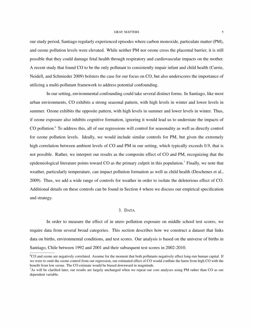
The seasonal patterns in pollution in Santiago are an important reason behind the inclusion of

month and year fixed effects in equation 1. As mentioned earlier, Figure 1 shows that there are strong

monthly patterns to CO and overall air quality as captured by the AQI. Since these seasonal patterns could

exist for other unmeasured variables that might impact our outcome of interest (e.g. income-specific timing

of childbirth), month fixed effects are an important control in all our specifications. Our approach requires

residual variation in the measures of pollution after controlling for seasonality (month fixed effects) and

year fixed effects. Figure 3 shows the distribution of CO after removing these fixed effects; we see that

substantial variation remains in the pollution measures. It is this variation that drives the identification in

this paper.

The first modification we make to equation 1 is the introduction of observable mother’s character-

istics. Hence, we estimate:

Sijrt = �Emt + ✓t + ↵�ijrt + �Wt + �Xj + ✏ijrt(2)

Where Xj includes mother’s characteristics like age and education.

The identifying assumption in the above equation is that after controlling for observable maternal

characteristics, seasonality and flexible weather controls, exposure to pollution is uncorrelated with ✏ijrt.

13Temperature controls are constructed as follows: for each trimester, we count days for which maximum temperature falls in eachof 6 10-degree F bins, 40-49, 50-59, 60-69, 70-79, 80-89, � 90.Thisresultsin3trimesters ⇤ 6bins = 18countvariables.14Recall that the correlation between CO and PM10 levels is 0.9 (see Appendix Table A1). Also, our results are not sensitive to theuse of ozone as a control variable. This is likely due to the fact that ozone and CO are inversely correlated and seasonal controls doenough to capture the effects of ozone.


One concern with this assumption is that parents may respond to pollution levels, either directly by limiting

exposure to pollution or indirectly through ex post investments designed to mitigate harmful effects. While

such responses would not bias our results, they imply that all estimates would capture pollution impacts

net of these potentially costly behaviors.15 To clarify the interpretation of � in our estimation strategy, it is

useful to describe a simple education production function.

We begin by specifying a production function for school achievement, similar in spirit to Todd

and Wolpin (2007). Test score achievement of student i born to mother j in region r at time t 16 is a

function of early childhood health (H), investments made from birth to time of test taking (P ) and parental

characteristics (X).

Sijrt = f(Hijrt,

k=TX

k=t

Pijrk, Xj)(3)

Early childhood health is a function of in utero pollution exposure E, weather conditions W (e.g.

rainfall, temperature, etc.) and parental characteristics X . Individual environmental conditions are a func-

tion of ambient pollution measured at the nearest monitor (Emt), mitigated by individual level avoidance

behavior (A).

Hijrt = h(Eijrt,Wijrt, Xj)(4)

Eijrt = e(Emt, Aijrt)(5)

Taking a linear approach to estimating equation 3 and plugging in linear functions of equations 4

and 5, and recognizing that weather variables are observed at the city wide, we can express student perfor-

mance as:

Sijrt = �Emt + �Wt +k=TX

k=t

⌫kPijrk + ⌘Aijrt + �Xj + ✏ijrt(6)

Equation 1 is essentially a modified version of equation 6. Test scores still depend on environmental

conditions and parental characteristics, and now also depend on time-varying parental investments in human

15See Graff Zivin and Neidell (2012) for a detailed conceptual model of the environmental health production function.16In our specification, t always refers to time of birth, not time of test taking. For the most part everyone born at time t takes thetest at the same later time (T ), since we use scores from the national fourth grade exam.

GRAY MATTERS 11

capital as well as pollution avoidance behaviors during the prenatal period. While educational investments

in response to early life insults are not observable in our setting (they will be subsumed in our error term),

studies in other similar contexts have found those responses to be small and if anything largely compensatory

(see Bharadwaj, Eberhard and Neilson (2013) and Halla and Zweimüller (2014)). Thus, to the extent that

Chilean parents make investments to overcome cognitive deficiencies due to in utero pollution exposure,

they will be reflected in our estimated effects from pollution. This is desirable - it captures the realized

impacts of pollution - but it is worth noting that the costs of those parental investments may constitute a

sizable welfare cost due to pollution.

Avoidance behavior can take two broad forms and we employ two main techniques to capture them

in our analysis. Since residential sorting can lead to non-random assignment of pollution, we employ sibling

fixed effects models to make within household comparisons that hold geography fixed. This is a particu-

lar concern as air quality is capitalized into housing values (Chay and Greenstone 2005, Figueroa, Rogat,

Firinguetti 1996). Families with higher income are more likely to sort into neighborhoods with better air

quality and invest in human capital.17 Sibling fixed effects in this setting also play an important role insofar

as our limited data on maternal characteristics is missing important unobservable family characteristics that

might matter for test outcomes as well as pollution exposure (Currie, Neidell, and Schmieder 2009). Our

estimating equation using sibling fixed effects (indexing another sibling i0 born at t0) is essentially a first

difference across siblings and takes the form:

�Sijrt�i0jrt0 = ��Emt�mt0 + ��Wt�t0 +�uijrt�i0jrt0(7)

In general the addition of granular fixed effects can exacerbate measurement error problems (Griliches

and Hausman 1986). In studies of air pollution exposure, however, a spatial error component is often the pri-

mary concern. If measurement error is an additively separable function of location, our sibling fixed effects

estimates will reduce rather than exacerbate bias from measurement error. In this vein, Jerrett et al (2005)

find that community fixed effects reduce attenuation in estimates of the pollution-mortality relationship. In

addition, our sibling fixed effects will capture all time-invariant investments in children. Equation (7) ig-

nores time-varying investments, however, since we do not have data on parental investments across siblings.

17Note that our results are robust to the inclusion of municipality (neighborhood) linear time trends.


One time-varying activity that may influence outcomes is averting behavior. In the short run, individuals can

take deliberate actions to reduce their realized exposure to pollution by spending less time outside, wear-

ing face masks, or engaging in a number of other activities (Neidell 2005, Neidell 2009). Such short-run

responses require knowledge about daily or even hourly pollution levels. In our context, that knowledge

is made available through a well-publicized system of air quality alerts based on PM10 levels (which are

highly correlated with CO levels). For example, during May-August, the peak pollution months in Santiago,

PM10 forecasts are broadcast on a regular basis, with alerts announced when this pollutant reaches certain

thresholds (see Mullins and Bharadwaj 2014 for details). To the extent that these alerts generate behavioral

responses, we can account for them by including controls for the number of alert days during the pregnancy

for each trimester.18 If individuals engage in avoidance behavior, controlling for avoidance should make

the estimates larger relative to estimates where this is not explicitly taken into account (Moretti and Neidell

2011). These avoidance controls also reduce exposure measurement error arising from differences in indoor

and outdoor air quality (Zeger et al 2000).

We modify equation 7 to take transient avoidance into account as follows:

�Sijrt�i0jrt0 = ��Emt�mt0 + ��Wt�t0 + �Alertst�t0 +�uijrt�i0jrt0(8)

All of our core analyses will follow the same basic structure. The OLS regression described in equation

(2) will serve as our base model specification. This will be followed by estimates of the sibling fixed effect

regressions described in equation (7). Finally, we will present estimates of our fully saturated model, which

includes sibling fixed effects and controls for air quality alerts to capture time-varying avoidance behavior,

as described in equation (8).

5. RESULTS

We begin our analysis by examining the impact of CO on test scores in Table 2. Panel A presents

the estimates using 4th grade math scores as the dependent variable and Panel B uses 4th grade language

scores as the dependent variable. Column 1 is our base OLS specification where we control for seasonality

18Of course, individuals may also engage in avoidance behavior based on the visible signs of pollution (or its correlates). While wecannot control for those behaviors in this setting, they can be viewed as conceptually similar to unmeasured parental investmentsin human capital. They create a wedge between the “biological” and “in situ” impacts of pollution, and represent a potentiallysignificant welfare cost attributable to pollution.

GRAY MATTERS 13

(year and month fixed effects interacted with monitor dummies), environmental controls at the trimester

level (maximum temperature in 10 degree F bin days and a second degree polynomial in mean precipitation,

fog, wind speed and dew point), demographic controls (mother’s age and education, student gender) and

trimester average ozone levels.19 Standard errors are clustered on family and municipality (neighborhood)

in all columns. We add to this base model, sibling fixed effects in column 2 and further add the total number

of trimester level air quality alert days in column 3.

Table 2 Panel A shows negative and significant effects of in utero CO exposure on 4th grade math

test scores in specifications that account for sibling fixed effects.20 The effects are concentrated in trimesters

2 and 3 (although estimates for trimester 2 are not statistically significant). Moving from Column 1 to

Column 2 illustrates the importance of accounting for sorting behavior and other time-invariant unobserved

family characteristics in this setting, as the magnitudes of our estimates increase significantly in Column 2.

A 1 SD increase in CO in the third trimester is associated with a statistically insignificant 0.005 SD decrease

in 4th grade math scores (column 1); however adding sibling FE in Column 2 increases the magnitude to a

statistically significant 0.034 SD. Adding air quality alerts to our sibling fixed effects specification (Column

3) increases the magnitude of the estimates slightly (by about 6 to 8 percent in most cases), suggesting

that insofar as the alerts induce avoidance behavior, this appears to have a rather modest impact on child

outcomes.21 Panel B shows similar effects in both direction and magnitude on language test scores.

Taken as whole, the results in Table 2 reveal a strong negative effect from fetal exposure to CO.22

While the magnitudes may appear small, it is important to note that test performance is notoriously difficult

to move, even via input-based schooling policies (Hanushek 2003). To place the magnitudes of these ef-

fects in context, they are roughly one-fifth the magnitude of successful interventions that specifically target

educational outcomes in developing countries (JPAL 2014). The economic importance of these results is

19As discussed in Section 2, this study focuses on CO rather than ozone because the scientific literature documents the mechanismby which CO harms a developing fetus. Ozone may also be harmful to the fetus, but the mechanisms are unknown. Appendix TableA3 reports the estimated ozone coefficients from our preferred specification.20As described later in this section, our results remain qualitatively similar when we repeat our core analysis replacing CO withPM10 or with AQI.21The difference in coefficients from adding the alerts controls is similar for trimesters 2 and 3. We caution against over-interpretingthis pattern, however. First, these differences are very small relative to the associated standard errors. Second, these differencesreflect both the quantity of avoidance behavior and its effectiveness, which could vary over the course of a pregnancy.22An alternative measure is to measure pollution over the entire 9 months of the pregnancy. This measure yields similar negativeand significant effects as seen in the graphs in Appendix Figures A1 and A2.


underscored by the size of the exposed population – far more children are exposed to pollution than well-

designed education-specific programs in developing countries. It is also worth noting that our effects are

quite a bit larger than estimates based on changes in total suspended particulates pollution within the U.S.

(Sanders 2012). 23

In Table 3, we examine heterogeneity in these human capital impacts by mother’s education. For

both math and language test scores, we see that the effects of CO exposure are quite a bit larger for children

of mothers without a high school diploma. A 1 SD increase in third trimester CO affects the children of

less educated mothers by more than twice as much as the children of more educated mothers (columns 3

and 6). These results provide suggestive evidence that less educated families are more vulnerable to the

detrimental effects of pollution. There are several possible explanations for this pattern, including but not

limited to: 1) increased susceptibility, perhaps due to poorer baseline health; 2) increased exposure; and 3)

diminished ability to invest in children to offset early life deficits. The relative importance of these and other

mechanisms remains an open question.

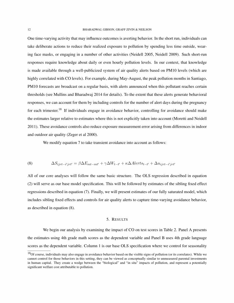
All of our previous analysis treated the relationship between CO exposure and test scores as linear.

Figures 4 and 5 show the relationship between pollution and test scores for the third trimester of pregnancy

using local linear regressions. The figures confirm the negative result found in the previous tables and sug-

gest non-linearity is not first order in this setting. However, we note that there are many ways to model

non-linearity in this context. In order to avoid ad-hoc searches for non-linearity, we adopt counts of vio-

lations of the U.S Environmental Protection Agency’s National Ambient Air Quality thresholds for CO (9

parts-per-million for an 8-hr average)24 as our non-linear exposure measure. To be clear, for each trimester

we sum the number of days on which the EPA’s safety threshold is exceeded. Table 4 presents these results

for both math and language. We find that for every extra day of EPA threshold violation during the third

trimester, test scores decrease significantly, with a consistent magnitude around 0.003 SD using the fixed

effects estimates. It is worth noting that violations of the EPA standard were a regular occurrence in the

1990s in Santiago. For example, in 1997 approximately 47 days exceeded the EPA CO limit, which, lin-

early would imply an effect of nearly 0.15SD if all 47 violations happened in the second or third trimester.

The average number of EPA violations during a third trimester in our sample is 2.3, which translates to a

23The estimates in Sanders (2012) may be smaller due to measurement error issues. Sanders (2012) infers in utero pollutionexposure by assuming all students were born in the place they attended high school.24The average CO levels over a trimester in our sample is approximately 1 part-per-million.

GRAY MATTERS 15

0.007 SD reduction in test scores for the average child exposed to such a third trimester. Appendix Table

A4 adopts an alternative approach to non-linearity, allowing CO exposure to enter as counts of 3rd-trimester

days in four bins. Consistent with our findings in Table 4, there is suggestive evidence that harmful effects

stem from the most polluted days, with ambient readings over 3.3ppm.

Thus far our analysis has largely been silent on the various mechanisms that might underpin our

results. While our data do not allow us to formally disentangle possible channels, they do allow us to probe

an important one. Since birth weight has been shown to be an important determinant of school performance

(Figlio et al. 2013, Bharadwaj et al. 2013), we directly explore the effects of in utero pollution exposure on

birth weight in a specification similar in spirit to Equations 7 and 8. Our OLS specification in Table 5 shows

that exposure to in utero pollution significantly decreases birth weight. The magnitude of these effects is

amplified in the sibling FE framework, which also finds modest and marginally significant effects on the

probability of being low birth weight (less than 2500 grams). While these results suggest that some of the

long term effects seen are via the channel of health at birth, it is important to note that these birth weight

effects are much too small to explain all of the relationship between pollution and scores. Indeed, point

estimates from Bharadwaj, Eberhard and Neilson (2013) of the impact of birthweight on test scores imply

that this channel explains no more than 10% of the cognitive impacts due to pollution.

5.1. Robustness Checks

As mentioned earlier, due to the high correlation between CO and PM10, our main specifications

do not control for PM10. Hence, replacing CO with PM10 should yield qualitatively similar results. In Table

6, we find that this is indeed the case. Across all three of our specifications, we find that exposure to PM10

in utero is associated with significant negative effects on 4th grade math and language scores. An alternative

approach to addressing multiple pollutants is to aggregate them into a single index. In this case, we use

the U.S. Environmental Protection Agency’s Air Quality Index (AQI), which is constructed by taking the

maximum over piecewise-linear transformations of daily readings for all individual pollutants (EPA, 2006).

As can be seen in Table 7, higher AQI exposure in utero leads to lower test scores. While this approach does

not allow us to disentangle the effects of different pollutants, these results follow the same patterns as prior

tables – most of the effects are concentrated in the second and third trimester and the coefficients are larger

after accounting for sibling fixed effects.


Table 8 adds controls for family size at birth to our preferred specification. Because we do not

observe pre-1992 births, family size observed in our data will be weakly smaller than true family size at

birth. Note that this is equivalent to a birth order control, again with the caveat that we observe only relative

birth order within our data. Estimates from the specification with family size controls, implemented as a

series of dummy variables, are very similar to those from our preferred specification. Table 9 investigates

the role of movers in our analysis. We define a mover dummy that equals 1 for a mother observed in

two different municipalities (neighborhoods). Because our econometric analysis focuses on mothers with

multiple births, we have a relatively large fraction of movers in the sample at roughly 29%. In our sample,

just 3,374 children are born to mover families in Las Condes. Because readings at the La Independencia

and Parque O’Higgins monitors are similar, in most cases the pollution exposure we assign to a family does

not change substantially as a result of the move. In Table 9 the interactions of the mover dummy with CO

exposure are all negative, but small and not statistically significant at conventional levels.

Finally, Table 10 shows that CO exposure in trimesters prior to conception does not play a role

in determining test scores. This is important and reassuring, as it shows that our time dummies and other

controls are effective in capturing serial correlation in pollution exposure. Table 11 shows that in years after

birth, the effect of pollution is not generally statistically significant; however, the standard errors are too

large to conclude whether post natal exposure can truly be harmful or not. Future research on this topic

would be useful to shed light on the importance of post natal exposure, the role of avoidance behaviors

undertaken by parents after birth has occurred, and its impacts on human capital production.25

6. CONCLUSION

In this paper, we merge data from the Chilean ministries of health and education with pollution

and meteorological data to assess the impact of fetal air pollution exposure on human capital outcomes

later in life. Data on air quality alerts and the use of siblings fixed effects estimation allow us to address

several potentially important concerns about endogenous exposure to poor environmental quality. We find

a strong and robust negative effect from fetal exposure to CO on math and language skills. Our results are

also in line with the scientific literature suggesting the importance of the first and third trimester in fetal

brain development. Our richest model specification suggests that a 1 standard deviation increase in CO

25We also measure post natal exposure in trimesters, examining the impacts from post trimesters 1 to 6. The effects in the siblingbased specifications are insignificant and small in magnitude (results available upon request).

GRAY MATTERS 17

exposure during the third trimester of pregnancy is associated with a 0.036 standard deviation decrease in

4th grade math test scores and a 0.042 SD decrease in 4th grade language test scores. Given the inherent

challenges associated with improving education outcomes, these impacts are sizable - roughly one-fifth the

magnitude of successful interventions that directly target educational performance in developing countries

(JPAL 2014).

Since school performance is an important driver of employment and wage outcomes later in life

(Chetty et al 2011, Currie and Thomas 2012), the legacy of these acute pollution exposures in utero can be

long lasting and economically significant. In developing countries where pollution levels tend to be higher,

those impacts may be particularly large. In that regard, the dramatic transformation of air quality in Chile

from the early-1990s to the mid-2000s is instructive. During this period, which can be viewed as a transition

from typical developing country urban pollution levels to levels that are closer to those found in typical

developed country cities, average CO levels in Santiago dropped by more than 50 percent. A back-of-the

envelope calculation using our estimated human capital effects and estimates on the returns to test scores

from the U.S. (Blau and Kahn, 2005) suggests that, ceteris paribus, this drop could account for as much as

$1000 in additional lifetime earnings per child born under the cleaner regime. During our sample period

on average 100,000 children are born every year in Santiago, suggesting a lifetime increase of 100 million

USD per cohort.26 It is important to realize that most of the costs of pollution exposure might be borne

by the less fortunate. Such results may help explain patterns of wealth accumulation around the world,

where the poor tend to live in neighborhoods with low environmental quality, which diminishes cognitive

attainment and thus limits opportunities to rise out of poverty. The sizable non-pecuniary benefits from

education (Oreopoulos and Salvanes 2011) only serve to magnify these welfare impacts.

Our empirical results are also of direct importance for policy makers. Carbon monoxide is directly

regulated throughout the developed and an increasing share of the developing world. Nearly all of these reg-

ulations are based on the benefits associated with reductions in pollution-related health problems, mortality

26This number is calculated as follows. The change in average CO levels between 1992 and 2002 is equivalent to a 1 standarddeviation change in CO pollution levels. Using our sibling FE results for math performance in the third trimester (this is conser-vative, as the improvement we imagine will apply for the entirety of the pregnancy, rather than a specific trimester) implies thatthis change in pollution levels generates a 0.036 SD improvement in test scores. Blau and Kahn (2005) find that a 1 SD change inU.S. adult test scores averaged across math and verbal reasoning yields a 16.36 percent change in adult earnings after controllingfor education levels (see table 2, column 4 in Blau and Kahn 2005). Applying this relationship between U.S. adult test scores andearnings to Chilean children yields an annual wage increase of 0.58%. Finally, we apply this figure to average adult wages in Chile(around 11000 USD) and discount at a 5% rate over 30 years.


and hospitalizations.27 Our results suggest that such an approach underestimates regulatory benefits for at

least two reasons. First, it completely ignores the human capital effects, which have been largely invisible,

but may well rival the more dramatic health effects in magnitude since they affect a much broader swath

of the population. Second, it fails to account for the costs of short- and long-run avoidance behaviors for

which we find evidence. While our empirical framework does not allow us to assess the magnitude of these

costs, they have been found to be substantial in other settings (Graff Zivin et al., 2011). The degree to which

these “additional” benefits imply stricter regulation will, of course, depend upon the costs and effectiveness

of pollution reduction.28

While this paper provides new evidence in support of the fetal origins hypothesis and its lasting

legacy on human capital formation, many questions remain unanswered. From a scientific perspective, the

mechanisms behind these impacts remain murky. Our evidence suggests that birth weight is one important

channel for these impacts, but it offers only a partial explanation. In the realm of human behavior, much

more work is needed to understand the role that households play in shaping outcomes. The effects we

measure are net of any parental investments that take place between birth and test taking. The scale of

these investments as well as their costs and effectiveness are largely unknown. Do they vary by identifiable

household characteristics or over the lifecycle of a child? A deeper understanding of the persistence of these

effects within and across generations is of paramount importance. Together these comprise a future research

agenda.

27Two examples of such work in the context of Santiago, Chile are worth mentioning. The first is Dessus and O’Connon (2003)who examine the welfare implications of climate policy in Santiago by including health costs. The second is the work of Figueroa,Gomez-Lobo, Jorquera and Labrin (2012), who estimate the benefits due to reduced pollution in Santiago due to better public transitinfrastructure.28Gallego, Montero and Salas (2011) provide a cautionary tale about well intentioned policies aimed at reducing air pollution. Theyfind that transportation policies in Santiago and Mexico City increased carbon monoxide levels, which given our findings wouldimply a reduction in human capital formation.

GRAY MATTERS 19

REFERENCES

ALMOND, D., AND J. CURRIE (2011): “Killing me softly: The fetal origins hypothesis,” The Journal of Economic Perspectives,

pp. 153–172.

ALMOND, D., L. EDLUND, AND M. PALME (2009): “Chernobyl’s subclinical legacy: prenatal exposure to radioactive fallout and

school outcomes in Sweden,” The Quarterly Journal of Economics, 124(4), 1729–1772.

ARCEO-GOMEZ, E. O., R. HANNA, AND P. OLIVA (2012): “Does the Effect of Pollution on Infant Mortality Differ Between

Developing and Developed Countries? Evidence from Mexico City,” Discussion paper, National Bureau of Economic Research.

AUFFHAMMER, M., AND R. KELLOGG (2011): “Clearing the air? The effects of gasoline content regulation on air quality,” The

American Economic Review, pp. 2687–2722.

BHARADWAJ, P., J. EBERHARD, AND C. NEILSON (2013): “Health at Birth, Parental Investments and Academic Outcomes,”

Discussion paper, Working Paper.

BLACK, S. E. (1999): “Do better schools matter? Parental valuation of elementary education,” Quarterly journal of economics,

pp. 577–599.

BLACK, S. E., A. BÜTIKOFER, P. J. DEVEREUX, AND K. G. SALVANES (2013): “This is only a test? long-run impacts of

prenatal exposure to radioactive fallout,” Discussion paper, National Bureau of Economic Research.

BLAU, F. D., AND L. M. KAHN (2005): “Do cognitive test scores explain higher US wage inequality?,” Review of Economics and

Statistics, 87(1), 184–193.

CHAY, K. Y., AND M. GREENSTONE (2005): “Does air quality matter? Evidence from the housing market,” Journal of

political economy, 113(2), 376–424.

CHETTY, R., J. N. FRIEDMAN, N. HILGER, E. SAEZ, D. W. SCHANZENBACH, AND D. YAGAN (2011): “How does your

kindergarten classroom affect your earnings? Evidence from Project STAR,” The Quarterly Journal of Economics, 126(4), 1593–

1660.

CUNHA, F., AND J. J. HECKMAN (2008): “Formulating, identifying and estimating the technology of cognitive and noncognitive

skill formation,” Journal of Human Resources, 43(4), 738–782.

CURRIE, J., ET AL. (2011): “Traffic Congestion and Infant Health: Evidence from E-ZPass,” American Economic Journal: Applied

Economics, 3(1), 65–90.

CURRIE, J., J. GRAFF ZIVIN, K. MECKEL, M. NEIDELL, AND W. SCHLENKER (2013): “Something in the water: contaminated

drinking water and infant health,” Canadian Journal of Economics/Revue canadienne d’économique, 46(3), 791–810.

CURRIE, J., AND R. HYSON (1999): “Is the impact of health shocks cushioned by socioeconomic status? The case of low

birthweight,” Discussion paper, National Bureau of Economic Research.

CURRIE, J., M. NEIDELL, AND J. F. SCHMIEDER (2009): “Air pollution and infant health: Lessons from New Jersey,” Journal

of health economics, 28(3), 688–703.

CURRIE, J., AND D. THOMAS (2012): Early test scores, school quality and SES: Long run effects on wage and employment

outcomes, vol. 35. Emerald Group Publishing Limited.


CURRIE, J., J. S. G. ZIVIN, J. MULLINS, AND M. J. NEIDELL (2013): “What Do We Know About Short and Long Term Effects

of Early Life Exposure to Pollution?,” Discussion paper, National Bureau of Economic Research.

CUTTER, W. B., AND M. NEIDELL (2009): “Voluntary information programs and environmental regulation: Evidence from

"Spare the Air",” Journal of Environmental Economics and Management, 58(3), 253–265.

DESCHÊNES, O., M. GREENSTONE, AND J. GURYAN (2009): “Climate change and birth weight,” The American Economic

Review, pp. 211–217.

DESCHENES, O., M. GREENSTONE, AND J. S. SHAPIRO (2012): “Defensive investments and the demand for air quality: Evi-

dence from the nox budget program and ozone reductions,” Discussion paper, National Bureau of Economic Research.

DESSUS, S., AND D. O’CONNOR (2003): “Climate policy without tears cge-based ancillary benefits estimates for Chile,” Envi-

ronmental and Resource Economics, 25(3), 287–317.

DIX-COOPER, L., B. ESKENAZI, C. ROMERO, J. BALMES, AND K. R. SMITH (2012): “Neurodevelopmental performance

among school age children in rural Guatemala is associated with prenatal and postnatal exposure to carbon monoxide, a marker

for exposure to woodsmoke,” Neurotoxicology, 33(2), 246–254.

DIZIK, A. (2013): “Does your child really need a private tutor,” BBC News: Capital, p. October 16.

DOBBING, J., AND J. SANDS (1973): “Quantitative growth and development of human brain,” Archives of Disease in Childhood,

48(10), 757–767.

ENSMINGER, M. E., AND A. L. SLUSARCICK (1992): “Paths to high school graduation or dropout: A longitudinal study of a

first-grade cohort,” Sociology of education, pp. 95–113.

EPA (2006): “Guidelines for the reporting of air quality - the Air Quality Index (AQI),” Discussion paper, US Environmental

Protection Agency, Office of Air Quality Planning and Standards.

FIGLIO, D. N., J. GURYAN, K. KARBOWNIK, AND J. ROTH (2013): “The Effects of Poor Neonatal Health on Children’s Cogni-

tive Development,” Discussion paper, National Bureau of Economic Research.

FIGUEROA, E., A. GÓMEZ-LOBO, P. JORQUERA, AND F. LABRÍN (2013): “Estimating the impacts of a public transit reform on

particulate matter concentration levels: the case of Transantiago in Chile,” Estudios de Economía, 40(1), JEL–Classification.

FIGUEROA, E., J. ROGAT, AND L. FIRINGUETTI (1996): “An estimation of the economic value of an air quality improvement

program in Santiago, Chile,” Estudios de Economia, 23(esp Year 1996), 99–114.

FREIRE, C., R. RAMOS, R. PUERTAS, M.-J. LOPEZ-ESPINOSA, J. JULVEZ, I. AGUILERA, F. CRUZ, M.-F. FERNANDEZ,

J. SUNYER, AND N. OLEA (2010): “Association of traffic-related air pollution with cognitive development in children,” Journal

of epidemiology and community health, 64(3), 223–228.

GALLEGO, F., J.-P. MONTERO, AND C. SALAS (2011): “The effect of transport policies on car use: Theory and evidence from

Latin American cities,” Documento de Trabajo IE-PUC, 407.

GARNIER, H. E., J. A. STEIN, AND J. K. JACOBS (1997): “The process of dropping out of high school: A 19-year perspective,”

American Educational Research Journal, 34(2), 395–419.

GRAY MATTERS 21

GRAFF ZIVIN, J., AND M. NEIDELL (2009): “Days of haze: Environmental information disclosure and intertemporal avoidance

behavior,” Journal of Environmental Economics and Management, 58(2), 119–128.

(2012): “The impact of pollution on worker productivity,” American Economic Review, 102, 3652–3673.

GRAFF ZIVIN, J., M. NEIDELL, AND W. SCHLENKER (2011): “Water quality violations and avoidance behavior: Evidence from

bottled water consumption,” Discussion paper, National Bureau of Economic Research.

GRAMSCH, E., F. CERECEDA-BALIC, P. OYOLA, AND D. VON BAER (2006): “Examination of pollution trends in Santiago de

Chile with cluster analysis of PM< sub> 10</sub> and Ozone data,” Atmospheric environment, 40(28), 5464–5475.

GRILICHES, Z., AND J. A. HAUSMAN (1986): “Errors in variables in panel data,” Journal of econometrics, 31(1), 93–118.

HALLA, M., AND M. ZWEIMÜLLER (2014): “Parental Response to Early Human Capital Shocks: Evidence from the Chernobyl

Accident,” Working Paper 1402, Department of Economics, University of Linz.

HANUSHEK, E. A. (2003): “The Failure of Input-based Schooling Policies*,” The economic journal, 113(485), F64–F98.

HECKMAN, J. J., L. J. LOCHNER, AND P. E. TODD (2006): “Earnings functions, rates of return and treatment effects: The Mincer

equation and beyond,” Handbook of the Economics of Education, 1, 307–458.

HUANG, H., R. XUE, J. ZHANG, T. REN, L. J. RICHARDS, P. YAROWSKY, M. I. MILLER, AND S. MORI (2009): “Anatomical

characterization of human fetal brain development with diffusion tensor magnetic resonance imaging,” The Journal of Neuro-

science, 29(13), 4263–4273.

IKONOMIDOU, C., F. BOSCH, M. MIKSA, P. BITTIGAU, J. VÖCKLER, K. DIKRANIAN, T. I. TENKOVA, V. STEFOVSKA,

L. TURSKI, AND J. W. OLNEY (1999): “Blockade of NMDA receptors and apoptotic neurodegeneration in the developing

brain,” Science, 283(5398), 70–74.

ISEN, A., M. ROSSIN-SLATER, AND W. R. WALKER (2014): “Every Breath You Take–Every Dollar Youï£¡ll Make: The Long-

Term Consequences of the Clean Air Act of 1970,” Discussion paper, National Bureau of Economic Research.

JERRETT, M., R. T. BURNETT, R. MA, C. A. POPE III, D. KREWSKI, K. B. NEWBOLD, G. THURSTON, Y. SHI, N. FINKEL-

STEIN, E. E. CALLE, ET AL. (2005): “Spatial analysis of air pollution and mortality in Los Angeles,” Epidemiology, 16(6),

727–736.

JPAL (2014): “Student Learning,” Downloaded April 2, 2014 from http://www.povertyactionlab.org/policy-

lessons/education/student-learning?tab=tab-background.

KNITTEL, C. R., D. L. MILLER, AND N. J. SANDERS (2011): “Caution, drivers! Children present: Traffic, pollution, and infant

health,” Discussion paper, National Bureau of Economic Research.

LUCAS, R. (1998): “On the mechanics of economic development,” ECONOMETRIC SOCIETY MONOGRAPHS, 29, 61–70.

MARGULIES, J. L. (1986): “Acute carbon monoxide poisoning during pregnancy,” The American journal of emergency medicine,

4(6), 516–519.

MINTZ, D. (2012): Technical Assistance Document for the Reporting of Daily Air Quality-the Air Quality Index (AQI). US Envi-

ronmental Protection Agency, Office of Air Quality Planning and Standards.


MORETTI, E., AND M. NEIDELL (2011): “Pollution, health, and avoidance behavior evidence from the ports of Los Angeles,”

Journal of human Resources, 46(1), 154–175.

MORTIMER, K., R. NEUGEBAUER, F. LURMANN, S. ALCORN, J. BALMES, AND I. TAGER (2008): “Air pollution and pulmonary

function in asthmatic children: effects of prenatal and lifetime exposures,” Epidemiology, 19(4), 550–557.

MULLINS, J., AND P. BHARADWAJ (2014): “Effects of Short-Term Measures to Curb Air Pollution: Evidence from Santiago,

Chile,” American Journal of Agricultural Economics, p. aau081.

NEIDELL, M. (2005): “Public information and avoidance behavior: Do people respond to smog alerts?,” Center for Integrating

Statistical and Environmental Science Technical Report, (24).

(2009): “Information, Avoidance behavior, and health the effect of ozone on asthma hospitalizations,” Journal of Human

Resources, 44(2), 450–478.

NILSSON, J. P. (2009): “The long-term effects of early childhood lead exposure: Evidence from the phase-out of leaded gasoline,”

Institute for Labour Market Policy Evaluation (IFAU) Work. Pap.

OREOPOULOS, P., AND K. G. SALVANES (2011): “Priceless: The nonpecuniary benefits of schooling,” The Journal of Economic

Perspectives, pp. 159–184.

OSSES, A., L. GALLARDO, AND T. FAUNDEZ (2013): “Analysis and evolution of air quality monitoring networks using combined

statistical information indexes,” Tellus B, 65.

OTAKE, M. (1998): “Review: Radiation-related brain damage and growth retardation among the prenatally exposed atomic bomb

survivors,” International journal of radiation biology, 74(2), 159–171.

PLOPPER, C. G., AND M. V. FANUCCHI (2000): “Do urban environmental pollutants exacerbate childhood lung diseases?,”

Environmental health perspectives, 108(6), A252.

RAU, T., L. REYES, AND S. S. URZÚA (2013): “The Long-term Effects of Early Lead Exposure: Evidence from a case of

Environmental Negligence,” Discussion paper, National Bureau of Economic Research.

REYES, J. W. (2007): “Environmental policy as social policy? The impact of childhood lead exposure on crime,” The BE Journal

of Economic Analysis & Policy, 7(1).

RIBAS-FITÓ, N., M. TORRENT, D. CARRIZO, L. MUÑOZ-ORTIZ, J. JÚLVEZ, J. O. GRIMALT, AND J. SUNYER (2006): “In

utero exposure to background concentrations of DDT and cognitive functioning among preschoolers,” American journal of epi-

demiology, 164(10), 955–962.

ROGAN, W. J., AND J. H. WARE (2003): “Exposure to lead in children-How low is low enough?,” New England Journal of

Medicine, 348(16), 1515–1516.

ROMER, P. M. (1986): “Increasing returns and long-run growth,” The journal of political economy, pp. 1002–1037.

SANDERS, N. J. (2012): “What doesn’t kill you makes you weaker prenatal pollution exposure and educational outcomes,” Journal

of Human Resources, 47(3), 826–850.

SANDERS, T., Y. LIU, V. BUCHNER, AND P. B. TCHOUNWOU (2009): “Neurotoxic effects and biomarkers of lead exposure: a

review,” Reviews on environmental health, 24(1), 15–46.

GRAY MATTERS 23

SCHLENKER, W., AND W. R. WALKER (2011): “Airports, air pollution, and contemporaneous health,” Discussion paper, National

Bureau of Economic Research.

TODD, P. E., AND K. I. WOLPIN (2007): “The production of cognitive achievement in children: Home, school, and racial test

score gaps,” Journal of Human capital, 1(1), 91–136.

VAN HOESEN, K. B., E. M. CAMPORESI, R. E. MOON, M. L. HAGE, AND C. A. PIANTADOSI (1989): “Should Hyperbaric

Oxygen Be Used to Treat the Pregnant Patient for Acute Carbon Monoxide Poisoning?,” JAMA: The Journal of the American

Medical Association, 261(7), 1039–1043.

WOODY, R. C., AND M. A. BREWSTER (1990): “Telencephalic dysgenesis associated with presumptive maternal carbon monox-

ide intoxication in the first trimester of pregnancy,” Clinical Toxicology, 28(4), 467–475.

ZEGER, S. L., D. THOMAS, F. DOMINICI, J. M. SAMET, J. SCHWARTZ, D. DOCKERY, AND A. COHEN (2000): “Exposure

measurement error in time-series studies of air pollution: concepts and consequences.,” Environmental health perspectives, 108(5),

419.

.51

1.5

22.5

3C

O (

ppm

)

1 2 3 4 5 6 7 8 9 10 11 12month

CO: Monthly

50

60

70

80

AQ

I

1 2 3 4 5 6 7 8 9 10 11 12month

AQI: Monthly

.51

1.5

22.5

CO

(ppm

)

1990 1995 2000 2005year

CO: Annual

50

60

70

80

AQ

I

1990 1995 2000 2005year

AQI: Annual

02

46

8C

O −

Independenci

a

01jan1

990

01jan1

992

01jan1

994

01jan1

996

01jan1

998

01jan2

000

01jan2

002

date

02

46

8C

O −

Parq

ue O

’Hig

gin

s

01jan1

990

01jan1

992

01jan1

994

01jan1

996

01jan1

998

01jan2

000

01jan2

002

date

02

46

8C

O −

Las

Condes

01jan1

990

01jan1

992

01jan1

994

01jan1

996

01jan1

998

01jan2

000

01jan2

002

date

0.2

.4.6

Densi

ty−5 0 5 10 15 20

Residualskernel = epanechnikov, bandwidth = 0.0971

CO

−.0

1−

.005

0.0

05

4th

gra

de m

ath

sco

re (

resi

dualiz

ed)

.8 1 1.2 1.4 1.6CO exposure (3rd trimester, residualized)

kernel = epanechnikov, degree = 1, bandwidth = .15

�

−.0

15

−.0

1−

.005

0.0

05

4th

gra

de la

nguage s

core

(re

sidualiz

ed)

.8 1 1.2 1.4 1.6CO exposure (3rd trimester, residualized)


�

⇤⇤ ⇤⇤

⇤⇤

⇤ ⇤⇤ ⇤⇤

�

⇤ ⇤ ⇤ ⇤

⇤⇤ ⇤⇤⇤ ⇤⇤⇤ ⇤⇤

⇤⇤ ⇤⇤

⇤ ⇤⇤⇤ ⇤⇤⇤ ⇤⇤⇤ ⇤⇤⇤ ⇤⇤⇤

�

⇤ ⇤

⇤⇤ ⇤⇤

⇤⇤

⇤⇤

⇤ ⇤⇤⇤ ⇤⇤⇤

�

⇤ ⇤

⇤⇤

⇤⇤ ⇤⇤⇤ ⇤

⇤ p < 0.10 ⇤⇤ p < 0.05 ⇤⇤⇤ p < 0.01

�

⇤ ⇤ ⇤

⇤⇤

⇤⇤

⇤⇤⇤ ⇤⇤ ⇤⇤

�

⇤⇤⇤

⇤ ⇤ ⇤

⇤⇤

⇤⇤⇤ ⇤⇤⇤ ⇤⇤⇤

⇤⇤⇤ ⇤⇤⇤ ⇤⇤

�

⇤⇤ ⇤⇤

⇤ p < 0.10 ⇤⇤ p < 0.05 ⇤⇤⇤ p < 0.01

�

⇤⇤ ⇤⇤

⇤ p < 0.10 ⇤⇤ p < 0.05 ⇤⇤⇤ p < 0.01

�

⇤

⇤ p < 0.10 ⇤⇤ p < 0.05 ⇤⇤⇤ p < 0.01

�

⇤⇤ ⇤⇤

⇤ p < 0.10 ⇤⇤ p < 0.05 ⇤⇤⇤ p < 0.01

�

−.0

2−

.01

0.0

1.0

24th

gra

de m

ath

sco

re (

resi

dualiz

ed)

1 1.2 1.4 1.6 1.8CO exposure (whole pregnancy, residualized)


�

−.0

15

−.0

1−

.005

0.0

05

.01

4th

gra

de la

nguage s

core

(re

sidualiz

ed)

1 1.2 1.4 1.6 1.8CO exposure (whole pregnancy, residualized)


�

⇤⇤ ⇤⇤

⇤ ⇤⇤

⇤ ⇤

⇤⇤ ⇤⇤ ⇤⇤

⇤

⇤⇤ ⇤

�

⇤⇤⇤ ⇤⇤⇤ ⇤⇤⇤

⇤⇤⇤ ⇤⇤ ⇤

�

⇤⇤⇤

⇤⇤ ⇤ ⇤⇤

⇤⇤⇤

⇤

�

Documents

GRAY MATTERS: FETAL POLLUTION EXPOSURE AND HUMAN CAPITAL FORMATIONweb.williams.edu/Economics/wp/BharadwajGibsonGraff… · · 2016-02-10GRAY MATTERS: FETAL POLLUTION EXPOSURE AND