JHEP03(2013)152

Published for SISSA by Springer

Received: January 11, 2013

Revised: February 26, 2013

Accepted: February 26, 2013

Published: March 27, 2013

Gravitating cosmic strings with flat directions

Betti Hartmann,a Asier Lopez-Eiguren,b Kepa Sousaa,b and Jon Urrestillab

aSchool of Engineering and Science, Jacobs University Bremen,

28759 Bremen, GermanybDepartment of Theoretical Physics, University of the Basque Country UPV/EHU,

48080 Bilbao, Spain

E-mail: b.hartmann@jacobs-university.de, asier.lopez@ehu.es,

k.sousa@jacobs-university.de, jon.urrestilla@ehu.es

Abstract: We study field theoretical models for cosmic strings with flat directions in

curved space-time. More precisely, we consider minimal models with semilocal, axionic

and tachyonic strings, respectively. In flat space-time, isolated static and straight cosmic

strings solutions of these models have a flat direction, i.e., a uniparametric family of config-

urations with the same energy exists which is associated with a zero mode. We prove that

this zero mode survives coupling to gravity, and study the role of the flat direction when

coupling the string to gravity. Even though the total energy of the solution is the same,

and thus the global properties of the family of solutions remains unchanged, the energy

density, and therefore the gravitational properties, are different. The local structure of the

solutions depends strongly on the value of the parameter describing the flat direction; for

example, for a supermassive string, the value of the free parameter can determine the size

of the space-time.

Keywords: Topological Strings, Classical Theories of Gravity, Supergravity Models

c© SISSA 2013 doi:10.1007/JHEP03(2013)152

JHEP03(2013)152

Contents

1 Introduction 1

2 The models and their flat directions 3

2.1 Semilocal strings 5

2.2 Axionic and tachyonic strings 7

3 Numerical results 10

3.1 Semilocal strings 11

3.2 Tachyonic strings or φ strings 13

3.3 Axionic strings or s-strings 15

4 Conclusions and discussion 17

1 Introduction

In several field theoretical models which allow for string-like objects it has been observed

that families of solutions which have different local behaviour of the fields appear, but

possess the same value of the energy per unit length. These zero modes do not disappear

when coupling the models minimally to gravity. Therefore, despite the fact that the global

properties of the family of solutions will remain unchanged, the gravitational properties

might change, since, after all, gravity is intrinsically locally defined.

The simplest model that is frequently used to describe cosmic strings is the U(1)

Abelian-Higgs model. The models we study in this paper are somewhat more complicated

than this one, but will be closely related to it since the solutions can (sometimes) be seen as

embedded Abelian-Higgs strings. Semilocal strings are solutions of an SU(2)global×U(1)localmodel which — in fact — corresponds to the Standard Model of Particle physics in the

limit sin2 θw = 1, where θw is the Weinberg angle. The simplest semilocal string solution

is an embedded Abelian-Higgs solution [1, 2]. A detailed analysis of the stability of these

embedded solutions has shown [3, 4] that they are unstable (stable) if the Higgs boson

mass is larger (smaller) than the gauge boson mass. In the case of equality of the two

masses, the solutions fulfill a Bogomolnyi-Prasad-Sommerfield (BPS) [5] bound such that

their energy per unit length is directly proportional to the winding number. Interestingly, it

has been observed [3, 4] that in this BPS limit, it is possible to find a one-parameter family

of single static and straight cosmic string solutions: the Goldstone field can form a non-

vanishing condensate inside the string core and the energy per unit length is independent

of this value, which itself is related to the width of the string. These solutions are also

sometimes denominated “skyrmions” and have been related to the zero mode associated

with the width of the semilocal strings present in the BPS limit. Semilocal strings have

– 1 –

JHEP03(2013)152

been studied in cosmological settings both in the context of their formation [6–9], network

properties [10] and their CMB implications [11].

The second model that we are investigating in this paper is a field theoretical model for

so-called axionic and tachyonic strings. This model, introduced in Blanco-Pillado et al. [12],

originally describes an unstable D-brane anti-D–brane pair and allows for the existence of

non-singular BPS strings. In fact, depending on the boundary conditions imposed on

the matter fields, the model accommodates three different types of strings [13]: φ-strings

(tachyonic), s-strings (axionic), and a hybrid of both types. As in the semilocal model,

each of these types of strings has a family of solutions of the same energy parametrized by

one parameter. For tachyonic and axionic strings, respectively, this parameter is associated

with the “width” of the strings - very similar to what happens in the semilocal model. On

the other hand, for hybrid strings it measures the contribution of the tachyonic string in

relation to the axionic string. These strings, in particular the tachyonic strings, share some

qualitative features with semilocal strings.

The gravitational properties of field theoretical cosmic string solutions have also been

discussed in the literature. The most thorough study has been done for Abelian-Higgs

strings by minimally coupling the Abelian-Higgs model to gravity [14, 15]. Far away from

the core of the string, the space-time has a deficit angle, i.e. corresponds to Minkowski

space-time minus a wedge [16]. The deficit angle is proportional to the energy per unit

length of the string. If the vacuum expectation value (vev) of the Higgs field is sufficiently

large (corresponding to very heavy strings that have formed at energies bigger than the

GUT scale), the deficit angle becomes larger than 2π. These solutions are the so-called

“supermassive strings” studied in [17, 18] and possess a singularity at a maximal value

of the radial coordinate, at which the angular part of the metric vanishes. Gravitating

semilocal strings have first been studied in [19].

In this paper we reinvestigate the gravitating semilocal strings and point out further

details. Moreover, we investigate gravitating axionic and tachyonic strings focusing in all

cases on the role of the zero mode. Our paper is organised as follows: in section 2, we

describe the models and give the equations of motion. In order to simplify the calcula-

tions we will use a standard result in the context of supergravity theories: cosmic string

configurations preserving a fraction of the supersymmetries in a supergravity theory sat-

urate a BPS bound, and the corresponding Einstein equations admit a first integral, the

so called gravitino equation, (see for example [20]). The models we will discuss here can

be embedded in N = 1 supergravity, [12, 21], and moreover the corresponding cosmic

string solutions leave unbroken half of the supersymmetries of the original theory. Here,

following the results in [22], we will rederive the first integrals of the Einstein equations for

the present models treating them as non-supersymmetric theories, and therefore, without

making any explicit reference to supersymmetry. The rest of the field equations will be

obtained using a BPS-type of argument valid for static cylindrically symmetric configura-

tions in a gravitational theory, that is, searching for the conditions required to minimize

an appropriate energy functional. The resulting equations will turn out to be a set of first

order differential equations for both models analog to those found in flat space-time [2, 12],

and in particular we recover the results already found in [19] for the semilocal case.

In section 3 we discuss the numerical results and conclude in section 4.

– 2 –

JHEP03(2013)152

2 The models and their flat directions

The models we are studying have an action of the following form

S = −1

2M2

p

∫

d4x√

−det g R+

∫

d4x√

−det gLm , (2.1)

where the gravitational strength coupling is given in term of the reduced Plank mass

M−2p = 8πG. The space-time metric has signature (−,+,+,+). The Ricci tensor scalar

follows conventions from [20].

We will study two types of matter Lagrangians Lm, the semilocal model [1, 2], and the

axionic D-term model presented in [12]. First we will discuss the gravity part of the model

and then we will describe the matter content in the subsections below. In particular, we

will point out what type of string-like solutions these models can accommodate and discuss

the role that gravity plays in connection to the zero modes.

In the present work we will focus on static cylindrically symmetric configurations

invariant under boosts along the axis of symmetry which, without loss of generality, we can

take to be the z−axis. The most general line element consistent with these symmetries is:

ds2 = −N2(r)dt2 + dr2 + L2(r)dϕ2 +N2(r)dz2 , (2.2)

where (r, ϕ, z) are cylindrical coordinates. The non-vanishing components of the Ricci

tensor Rνµ then read [14]:

R00 =

(LNN ′)′

N2L, Rr

r =2N ′′

N+

L′′

L, Rϕ

ϕ =(N2L′)′

N2L, Rz

z = R00 , (2.3)

where the prime denotes the derivative with respect to r. With our conventions the Einstein

equations have the following form

Rµν = −M−2p

(

Tµν −1

2gµνT

)

, (2.4)

where T = T σσ is the trace of the energy-momentum tensor which is given by

Tµν = −2∂Lm

∂gµν+ gµνLm . (2.5)

In [22] it was shown that the energy momentum tensor of the semilocal model has a very

simple form for field configurations satisfying the BPS bound. In particular, the only non-

vanishing components of T νµ are proportional to the field strength of an auxiliary vector

field ABµ , which is a function of the gauge boson and the scalar fields involved in the

string configuration:

T rr = Tϕ

ϕ = 0, T tt = T z

z = ±L−1(∂rABϕ − ∂ϕA

Br ), (2.6)

As we shall see below this statement is also true for the axionic D-term string model

proposed in [12].

– 3 –

JHEP03(2013)152

If the energy-momentum tensor is of the form (2.6) the metric function N(r) becomes

a constant [23, 24], and thus choosing the coordinates conveniently, we can always set it to

one, N(r) ≡ 1. To obtain the equation of motion for the remaining metric function L(r)

we use the ϕϕ-component of (2.4) which reads

L′′

L= −M−2

p

(

Tϕϕ − 1

2T

)

=1

2M−2

p T . (2.7)

In order for the metric to be regular at the z−axis we need to impose the following bound-

ary conditions

L(0) = 0 , L′(0) = 1 . (2.8)

For cylindrically symmetric field configurations it is possible to choose a gauge where

the vector field ABµ satisfies AB

r = 0 and ABϕ = AB

ϕ (r) and therefore, as long as the BPS

bound is saturated, we can find a first integral to the Einstein equations:1

L′′ = ±M−2p (AB

ϕ )′ =⇒ L′ = 1±M−2

p ABϕ . (2.9)

Here the integration constant is fixed by the boundary conditions (2.8), since regularity

also requires that ABϕ (0) = 0. This first integral of the Einstein equations allows us to

express the deficit angle of the string configurations in terms of the asymptotic value of

the vector field ABµ [23]

δ = 2π(1− L′|r=∞) = ∓2πM−2p AB

ϕ |r=∞. (2.10)

In order to discuss the existence of zero-modes in these theories we need an appropriate

definition of the energy which is valid for general curved space-times. We use the same

definition as in [20], which is valid for time independent configurations, and is obtained

adding a Gibbons-Hawking term to the action:

E = −S − SGH, SGH = M2p

∫

∂M

√

−det g K. (2.11)

Here K is the trace of the second fundamental form of the metric gµν at the space-time

boundary ∂M, and gαβ is the metric induced at ∂M. Note that field configurations

minimizing this energy functional also extremize the action, and therefore are solutions to

the equations of motion [25]. In order to obtain a finite value for the energy we calculate

the integrals in (2.11) only over the plane orthogonal to the string, i.e. over the r and ϕ

coordinates. Then, choosing the boundary to be a cylinder centered on the z−axis with

an arbitrary large radius r → ∞ we have (after setting N(r) = 1)

√

−det g K = L′(r), (2.12)

and thus the Gibbons-Hawking term can be written in terms of the deficit angle

SGH = M2p

∫

∂M

√

−det g K = 2πM2p

(

L′|r=∞ − L′|r=0

)

= −M2p δ. (2.13)

1In the context of supergravity theories this equation is know as the gravitino equation [20].

– 4 –

JHEP03(2013)152

Due to the Einstein equations, the action S vanishes on shell; and we find the following

relation between the energy of the string and its deficit angle:

E = M2p δ = ∓2π AB

ϕ |r=∞, (2.14)

where the second equality can be obtained using equation (2.10). In the following subsec-

tions we will arrive to the same result following a Bogomolnyi type of argument [5] which

involves rewriting the energy functional as a sum of positive terms plus a boundary term.

It is possible to show that for field configurations with the same symmetries as the

ones we discuss here the definition of the energy (2.11) agrees with the one used in [19],

E =

∫

d2x√

−det g T 00 . (2.15)

In order to check this is sufficient to note that using the ansatz for the metric (2.2), the

Einstein-Hilbert term becomes a boundary term which is exactly cancelled by SGH, and

that any contribution to the action involving time derivatives must be zero.

2.1 Semilocal strings

First, we will reconsider the semilocal model which possesses a SU(2)global×U(1)local sym-

metry [1, 2] and is given by the following matter Lagrangian density

LSLm = − (DµΦ)

†DµΦ− 1

4g2FµνF

µν − λ

2

(

ξ − Φ†Φ)2

, (2.16)

where Fµν = ∂µAµ − ∂νAµ is the field strength tensor of the U(1) gauge field and DµΦ =

(∂µ − iAµ)Φ is the covariant derivative of the complex scalar field doublet Φ = (φ1, φ2)T .

The constant g denotes the gauge coupling, λ the self-coupling of the scalar fields and√ξ

is their vacuum expectation value.

If the couplings satisfy the Bogomolnyi limit g =√λ, and working in the gauge

A0 = Az = 0, the energy functional (2.11) for the stationary string with a translational

symmetry along the z−axis can be given by

E =

∫

drdϕL(r)

[

(DrΦ)†DrΦ+ L−2 (DϕΦ)

†DϕΦ+1

2g2L−2FrϕFrϕ +

g2

2

(

ξ − Φ†Φ)2

]

,

(2.17)

which can be rearranged in the following way:

E =

∫

drdϕL(r)

[

(DrΦ± iL−1DϕΦ)†(DrΦ± iL−1DϕΦ)

+1

2g2

(

L−1Frϕ ∓ g2(ξ − Φ†Φ))2

]

∓∫

drdϕFBrϕ, (2.18)

where we have used the explicit form of the metric (2.2) after setting N(r) = 1, and we

have introduced the auxiliary vector field ABµ and its field strength:2

ABµ ≡ i

2(Φ†DµΦ−DµΦ

†Φ)− ξ Aµ, FBµν ≡ ∂µA

Bν − ∂νA

Bµ . (2.19)

2In the context of N = 1 supergravity, ABµ is known as the gravitino U(1) connection.

– 5 –

JHEP03(2013)152

In order to obtain finite energy configurations (2.17) we have to require that far away from

the center of the string the fields are in the vacuum, and that the covariant derivatives of

the fields vanish

Φ†Φ|r→∞ = ξ , DµΦ|r→∞ = 0 . (2.20)

Therefore, using Stokes’ theorem, we find the following lower bound for the energy of the

cosmic string

E ≥ ∓∫

drdϕFBrϕ = ±ξ

∫

drdϕFrϕ, (2.21)

where the last integral is the total magnetic flux trapped inside the string. Any field

configuration which saturates this bound is at a local minimum of the energy functional

and thus, as we argued in the previous subsection, it must be a solution to the equations of

motion. In particular, the bound is saturated by cosmic string configurations which satisfy

the BPS equations:

DrΦ± iL−1DϕΦ = 0, L−1 Frϕ ∓ g2(ξ − Φ†Φ) = 0. (2.22)

We use the following ansatz for a static straight cosmic string lying along the

z-axis [1, 2]:

φ1 =√

ξf(r)einϕ , φ2 =√

ξh(r)eimϕ , Aϕ = ±v(r), (2.23)

with all the other components of the gauge field set to zero. Here n and m are the

winding numbers of the fields φ1 and φ2 respectively and, without loss of generality, we

will assume3 |n| > |m|. By using the rescalings r → r/(g√ξ) and L(r) → L(r)/(g

√ξ) the

BPS equations read

f ′ +(v − |n|)

Lf = 0 , h′ +

(v − |m|)L

h = 0 ,v′

L+ (f2 + h2 − 1) = 0, (2.24)

which have to be solved subject to appropriate boundary conditions that result from im-

posing (2.20) and regularity at the origin [1, 2]

f2∞ + h2∞ = 1 , v(r → ∞) = |n| , (2.25)

f(0) = 0 , v(0) = 0 , h′m=0(0) = 0 or hm 6=0(0) = 0 , (2.26)

where f∞ = f(r = ∞) and h∞ = h(r = ∞). The choice of signs of the winding numbers

n and m in (2.24) ensures that these conditions can be met. Indeed, the BPS equa-

tions (2.22) with the upper sign can only be solved provided n,m > 0, while the lower sign

requires n,m < 0.

The first two BPS equations (2.24) imply that the profile functions f and h must be

related to each other [1, 2]

log h = log f − (|n| − |m|)∫

dr

L(r)+ κ =⇒ h = c · f · exp

(

(|m| − |n|)∫

dr

L(r)

)

(2.27)

3The case n = m can always be rotated into a Nielsen-Olesen string using a SU(2) transformation, and

therefore will not discuss it.

– 6 –

JHEP03(2013)152

and therefore, there is a one-parameter family of solutions characterized by a real constant

κ = log c . As in flat space, this family is degenerate in energy, i.e. the total energy does

not depend on the parameter κ. This can be checked inserting the ansatz for the gauge

boson (2.23) and its boundary conditions in (2.21):

E = ±ξ

∫

dϕAϕ|r=∞ = 2π|n|ξ . (2.28)

For field configurations safisfying the BPS equations (2.22) it is easy to check that the

energy momentum tensor takes the form (2.6), with ABµ given by (2.19). Then, the profile

function of the metric L(r) can be obtained from (2.9), which using the ansatz (2.23) takes

the form

L′ = 1− α2(

(|n| − v)f2 + (|m| − v)h2 + v)

, (2.29)

where α ≡ M−1p

√ξ is the vacuum expectation value of φ measured in Planck masses. From

the previous two equations it is possible to recover the relation (2.14) between the deficit

angle of the BPS strings and their energy

δ = M−2p E = 2π|n|α2 . (2.30)

Note that the choice of signs made above for the winding numbers ensures that the energy,

and thus the deficit angle, are positive.

2.2 Axionic and tachyonic strings

In this subsection we are going to consider the cosmic string solutions of the axionic

D−term model studied in flat space-time in [12, 13]. The model describes the dynam-

ics of two complex scalar fields, the tachyon φ, and an axio-dilaton S = s + ia (s > 0),

coupled to a U(1) gauge field Aµ. The lagrangian density reads

LAm = −DµφD

µφ−KSSDµSDµS − 1

4g2FµνFµν −

g2

2

(

ξ + 2δKS − qφφ)2

(2.31)

where Fµν = ∂µAν − ∂νAµ is the U(1) field strength, and the covariant derivatives of the

tachyon and the axio-dilaton are given by Dµφ = (∂µ − iqAµ)φ and DµS = ∂µS + i2δAµ

respectively. The model depends on three continuous parameters: the gauge coupling g,

the charge of the axio-dilaton δ, and ξ which determines the expectation value of the

fields. The constant q is an integer which represents the U(1) charge of the tachyon. The

lagrangian density also involves the derivatives of the Kahler potential associated with the

axio-dilaton field K(S, S), which is a real function chosen to have the following form:

K(S, S) = −M2p log(S + S). (2.32)

The quantities KS and KSS denote the derivatives of the Kahler potential with respect to

the fields S and S, and they are given by

KS = −M2p

1

S + S, KSS = M2

p

1

(S + S)2. (2.33)

– 7 –

JHEP03(2013)152

This lagrangian density is the bosonic part of a supersymmetric model with a D−term

scalar potential, and therefore the couplings satisfy the Bogomolnyi limit [26]. Thus,

without imposing further constraints in the couplings, the energy of a static configuration

E =

∫

drdϕL(r)

(

DrφDrφ+ L−2DϕφDϕφ+KSSDµSDµS

+1

2g2L−2FrϕFrϕ +

g2

2

(

ξ + 2δKS − qφφ)2

)

, (2.34)

can be written in the Bogomolnyi form as follows

E =

∫

drdϕL(r)

[

|Drφ± iL−1Dϕφ|2 +KSS |DrS ± iL−1DϕS|2

+1

2g2(

L−1Frϕ ∓ g2(ξ + 2δKS − q|φ|2))2

]

∓∫

drdϕFBrϕ , (2.35)

where we have defined the composite vector field ABµ and its field strength

ABµ ≡ i

2(φDµφ− φDµφ)−

iM2p

4 ReS(DµS −DµS)− ξAµ, FB

µν ≡ ∂νABµ − ∂µA

Bµ . (2.36)

As in the semilocal model, if we restrict ourselves to finite energy configurations, we have

to impose that far away from the string core the fields are in the vacuum, and that the

covariant derivatives vanish

(q|φ|2 − 2δKS)r→∞ = ξ , Dµφ|r→∞ , DµS|r→∞ = 0 . (2.37)

With these boundary conditions we find a lower bound for the energy similar to (2.21),

and the corresponding BPS equations (which ensure that the bound is saturated) read

(Dr±iL−1Dϕ)φ = 0, (Dr±iL−1Dϕ)S = 0, L−1 Frϕ∓g2(ξ+2δKS−q|φ|2) = 0. (2.38)

As we mentioned earlier in the paper, the energy momentum tensor reduces to a very

simple form for field configurations which satisfy the previous equations. Indeed, the only

non-vanishing components are given by

T tt = T z

z = ±L−1FBrϕ, (2.39)

and therefore as we discussed before the Einstein equations admit the first integral (2.9).

In order to solve the BPS equations we use the ansatz for the matter fields proposed

in [12], which represents a static straight cosmic string along the z−axis:

φ =√

ξ/q f(r)einϕ s−1(r) = ξ/(δM2p )h(r)

2

a = 2δ mϕ Aϕ = ±v(r) . (2.40)

After rescaling the radial coordinate and the metric profile function, r → r/(g√ξ), L →

L/(g√ξ), the BPS equations become:

f ′ +(qv − |n|)

Lf = 0, h′ + α2q

(v − |m|)L

h3 = 0,v′

L+ (f2 + h2 − 1) = 0, (2.41)

– 8 –

JHEP03(2013)152

where α = M−1p

√

ξ/q. The signs of the winding numbers n and m are fixed by requiring

f(r) to be regular and h(r)2 > 0 for r → 0. As in the semilocal case, we can use the first

two equations to find a relation between the tachyon and the dilaton field

1

(αh)2= 2 (|n| − q|m|)

∫

dr

L(r)− 2 log f + κ , (2.42)

and therefore the solutions are parametrized by an arbitrary constant κ. Actually, this

model admits three different families of cosmic string solutions depending on the boundary

conditions at r → ∞:

• φ-strings (tachyonic)

In this type of strings the magnetic flux trapped in the core is induced by the winding

of the tachyon field, which must satisfy |n| > q|m| in order to solve the BPS equations.

The profile functions have the following asymptotic behavior

f(r → ∞) → 1 , h(r → ∞) → 0 , v(r → ∞) → |n|/q (2.43)

so that the tachyon field acquires a non-vanishing expectation value far away from

the core while the function h(r) tends to zero. For the solutions to be regular we also

have to impose the following boundary conditions at the core of the strings r → 0:

f(0) = 0, v(0) = 0, h′m=0(0) = 0, or hm 6=0(0) = 0. (2.44)

In the present work we will only consider the case m = 0, where the profile function of

the axion-dilaton, h(r), can be non-zero at the core creating a “condensate”. Actually,

as in the flat space-time analysis [12], the value of h(r = 0) will be a free parameter

related to κ, which determines the width of the string. This family of solutions is

degenerate in energy

E = ±ξ

∫

dϕAϕ|r=∞ = 2π|n|ξq, (2.45)

and therefore the zero-mode survives the coupling to gravity. For simplicity, in our

numerical analysis we will set the constant q = 1.

• s-strings (axionic)

In this case the magnetic flux inside the strings is induced by the winding of the

axio-dilaton, S. The behaviour at infinity is

f(r → ∞) → 0 , h(r → ∞) → 1 , v(r → ∞) → |m| . (2.46)

It is now the dilaton which acquires a non-zero expectation value far from the core,

while the tachyonic field tends to zero far from the core. Thus, the role of the

tachyonic and the dilatonic field is exchanged. These strings are solutions to the

BPS equations provided |n| < q |m|. Regularity at the origin imposes the following

boundary conditions

h(0) = 0, v(0) = 0, f ′n=0(0) = 0, or fn 6=0(0) = 0. (2.47)

– 9 –

JHEP03(2013)152

In the next section we discuss the properties of this family of solutions for the case

n = 0, where the value of the profile function of the tachyon at the center of the

string, f(r = 0), is a free parameter related to κ. Again, this family of solutions is

degenerate in energy

E = ±ξ

∫

dϕAϕ|r=∞ = 2π|m|ξ, (2.48)

and thus the zero-mode still exists after coupling the model to gravity. Note that

s−strings have a tension q times larger than φ−strings. As for the tachyonic strings,

we will restrict the analysis to the case q = 1.

• Hybrid-strings

In this case, both the tachyon and the dilaton field contribute to cancel the scalar

potential far away from the core, i.e., they both acquire a finite vacuum expectation

value for r → ∞. This can only happen provided the windings satisfy |n| = q |m|.Thus, in this case we have the following boundary conditions at infinity

f2∞ + h2∞ = 1 , v(r → ∞) =

|n|q

= |m| , (2.49)

where f(r → ∞) ≡ f∞ and h(r → ∞) ≡ h∞. Provided the previous constraints are

satisfied, the value of f∞ is a free parameter, which will be again related to κ. In

this case κ is not a measure of the width of the string, instead, it is related to the

relative contributions of the tachyonic and the axionic string to the tension of the

string. The corresponding boundary conditions at the core of the string are given by

f(0) = 0, v(0) = 0, h(0) = 0. (2.50)

The zeromode associated with the parameter κ is not normalizable and thus we will

not discuss it any further in the present work. Indeed, if we promote the parameter

κ to be time dependent the corresponding effective action for the zeromode gets a

quadratically divergent contribution Λ2, where Λ is a cutoff which, in a cosmological

setting, could be given by the distance to the closest cosmic string.

Finally, the form of the equation for the metric profile function (2.9) can be found

using the ansatz (2.40):

L′ = 1− α2[

(|n| − qv)f2 + q(|m| − v)h2 + qv]

. (2.51)

Similarly to the semilocal case, from the boundary conditions discussed above, it is

straightforward to find a relation between the deficit angle of these strings and their en-

ergy: δ = M−2p q E.

3 Numerical results

We have solved the BPS equations for both models, subject to appropriate boundary

conditions, focusing on the interplay between the flat direction and gravity, in order words,

we studied how the local field configuration changed the energy density and the properties

of the solutions, even though the global energy was unchanged.

– 10 –

JHEP03(2013)152

0

0.5

1

1.5

2

0 2 4 6 8 10

r

fhvL

0

0.5

1

1.5

2

0 2 4 6 8 10

r

fhvL

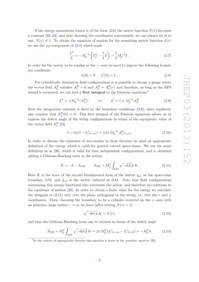
Figure 1. Profiles of a typical n = 1 semilocal string solution uncoupled to gravity, with different

values of the free parameter: h(0) = 0.1 (left) and h(0) = 0.9 (right).

0

0.5

1

1.5

2

0 2 4 6 8 10

r

fhvL

0

0.5

1

1.5

2

0 2 4 6 8 10

r

fhvL

Figure 2. The profiles of a gravitating n = 1 semilocal string (α = 0.5) with the value of the free

parameter h(0) = 0.1 (left) and h(0) = 0.9 (right).

3.1 Semilocal strings

The gravitating properties of semilocal strings were first studied in [19]. Besides completing

that analysis, we include this case in the present work because it shares several properties

with the other cases to be studied.

Figure 1 shows two typical n = 1 cosmic string solutions to this model, when the

coupling to gravity is not included. The metric function L ≡ r in this case. These figures

illustrate the effect of varying the value of the condensate h at the center of the string

r = 0, i.e. the free parameter of the family of degenerate solutions. For larger values of

h(r = 0) the profile functions reach their asymptotic values farther away from the center

of the string and thus, as we anticipated in the previous subsection, the width of the string

core increases.

The form of the profiles when coupling to gravity, can be seen in figure 2. Close to the

core, the profile functions have the same form as in a Minkowski background:

L(r) ≈ r + . . . , f(r) ≈ f0 r|n| + . . . , h(r) ≈ h0 r

|m| + . . . , v(r) ≈ 1

2r2 + . . . .

(3.1)

However, far away from the core, r → ∞, the metric takes the form

ds2 ≈ −dt2 + dr2 + (1− |n|α2)2 r2dϕ2 + dz2, (3.2)

– 11 –

JHEP03(2013)152

0

1

2

3

4

5

6

7

8

9

10

0 2 4 6 8 10

L(r)

r

α=0.0α=0.5α=1.0

α=1.02

0

2

4

6

8

10

12

14

0 2 4 6 8 10 12 14

L(r)

r

h(0)=0.1h(0)=0.5h(0)=0.9

Figure 3. The function L for different configurations. On the left, h(0) = 0.5 while we vary the

values of α; on the right α = 0.5 while we vary the value of h(0).

0

0.1

0.2

0.3

0.4

0.5

0.6

0.7

0.8

0.9

0 2 4 6 8 10 12 14

L(r)

xΕ

r

h(0)=0.1h(0)=0.5h(0)=0.9

Figure 4. Energy density for different values of the free parameter h(0), with fized α = 0.5.

which corresponds to a conical space-time with a deficit angle δ = 2π|n|α2, and the behavior

of the profile functions in the same limit is given by the following asymptotic expansion:

f(r) ≈ 1− 1

2

(

r

r0

)

2(|m|−|n|)

1−|n|α2

+ . . . ,

h(r) ≈(

r

r0

)

|m|−|n|

1−|n|α2

+ . . . ,

v(r) ≈ |n| − (|n| − |m|)(

r

r0

)

2(|m|−|n|)

1−|n|α2

+ . . . , (3.3)

where r0 is a parameter related to h0 which determines the width of the string core. Setting

the constant α = 0 we recover the corresponding expansions in flat space.

The figures show that the metric function L does indeed depend on the value of the

condensate. We can see the dependence more clearly in the right plot of figure 3 where we

have displayed the metric function L for different values of the condensate keeping constant

the value of α. In the left plot of figure 3 we show the profile function L in different cases

where we keep the value of the condensate constant and vary the value of the α parameter.

Note that the deficit angle (2.10) increases with increasing α, and also that as α approaches

zero, the space-time becomes Minkowski, where L(r) = r.

One way of understanding this phenomenon is by looking at the energy density for

each one of these configurations, as shown in figure 4, where we only vary the value of the

– 12 –

JHEP03(2013)152

0

50

100

150

200

250

0 0.1 0.2 0.3 0.4 0.5 0.6 0.7 0.8 0.9 1

r*

h(0)

Figure 5. Values r∗ at which the function L = 0 for a given coupling constant (α = 1.02) with

respect to the value of the condensate at the core h(0).

condensate. Even though the total energy (the area below these lines) is the same, the

energy density is different, and affects the metric function with different strength. Indeed,

since the width of the string core increases with the value of the condensate, the energy

density spreads and the metric profile function L reaches its asymptotic behavior farther

away from the string. Note also that the deficit angle for each of the configurations is

exactly the same, and therefore the slope of the profile function L in the limit r → ∞should be the same regardless of the value of the condensate.

For BPS cosmic strings the energy density is closely related to the magnetic field Frϕ

E(r) = ξv′(r)

L, (3.4)

and thus from (3.1) and (3.3) it is trivial to find the limiting form of the energy density

E(r → 0) ≈ ξ

2+ . . . , E(r → ∞) ≈ 2ξ(|n| − |m|)2

(1− |n|α2)2r2

(

r

r0

)

2(|m|−|n|)

1−|n|α2

+ . . . . (3.5)

A dramatic effect happens when considering supermassive strings. In this case the

string is massive enough to make the function L turn round and become zero at some

finite value of r∗ (see Fig 3 for the case with α = 1.02), in other words, the deficit angle

δ becomes larger than 2π. The value of the condensate in the core determines the extent

to which this solution exists; it decides the “size” of the universe. Once again, the total

energy does not change, i.e., the integral for the energy density curve from r = 0 up to

the other point r∗ where L(r∗) = 0 is independent of the value of h(r = 0). In figure 5

we have depicted the values of r∗ for a fixed coupling constant with respect to the value of

the condensate at the core h(r = 0). As the value of the condensate increases the string

core (where space-time is approximately Minkowski) becomes wider. In the limiting case

where h(r = 0) → 1 the space-time becomes Minkowski everywhere and the point r∗ tends

to infinity.

3.2 Tachyonic strings or φ strings

These solutions share many properties with the semilocal strings, the main difference being

the factor of h3 in the equation (2.41) instead of the h in equation (2.24). This translates

– 13 –

JHEP03(2013)152

0

0.5

1

1.5

2

0 2 4 6 8 10

r

fhvL

0

0.5

1

1.5

2

0 2 4 6 8 10

r

fhvL

Figure 6. Profiles of a gravitating tachyonic string (α = 0.5) with the value of the free parameter

h(0) = 0.1 (left) and h(0) = 0.9 (right).

into the function h tending to zero logarithmically. As in the semilocal case, the tachyonic

field f is responsible for the formation of the string, whereas h is responsible for the

condensate. Close to the core of the string the profile functions behave as in flat space-

time [12], in particular

f(r) ≈ f0 r|n| + . . . , h(r)−2 ≈ h−2

0 − 2α2q|m| log r+ . . . , v(r) ≈ 1

2r2 + . . . . (3.6)

The value h(0) is a free parameter, related to the string width, which leaves the total

energy unchanged and modifies the field configurations slightly. A typical n = 1 cosmic

string configuration can be seen in figure 6, which shows that, as in the case of semilocal

strings, for larger values of the condensate the core width increases. Note also how the

h field tends to zero slowly. Actually, all the profile functions approach their values at

infinity logarithmically, as can be seen from their asymptotic expansion

h(r)2 ≈ (1− |n|α2)

2α2(|n| − q|m|) log r + . . . ,

f(r) ≈ 1− (1− |n|α2)

4α2(|n| − q|m|) log r + . . . ,

v(r) ≈ |n|q

− (1− |n|α2)2

4α2q(|n| − q|m|) log2 r + . . . . (3.7)

The term appearing in the numerator of the three expressions (1−|n|α2) was not obtained

in the flat space-time analysis done in [12], since this is a consequence of the asymptotic

form of the space-time metric

ds2 ≈ −dt2 + dr2 + (1− |n|α2)2 r2dϕ2 + dz2. (3.8)

From (3.7) we can immediately extract the form of the energy density far away from

the core:

E(r) =M2

p (1− |n|α2)

2(|n| − q|m|)r2 log3 r + . . . . (3.9)

Most of our results for the semilocal strings can also be obtained here. The global

energy, and thus the deficit angle, are independent of the value of the h field at r = 0,

implying that the slope of L remains unchanged for large values of r; however, as the energy

– 14 –

JHEP03(2013)152

0

0.1

0.2

0.3

0.4

0.5

0.6

0.7

0.8

0.9

0 5 10 15 20 25 30 35

L(r)

xΕ

r

h(0)=0.1h(0)=0.5h(0)=0.9

Figure 7. Energy density for different values of the free parameter h(0) with fixed α = 0.5.

0

1

2

3

4

5

6

7

8

9

10

0 1 2 3 4 5 6 7 8 9 10

L(r)

r

α=0.0α=0.9α=1.2

0

2

4

6

8

10

12

14

0 2 4 6 8 10 12 14

L(r)

r

h(0)=0.1h(0)=0.5h(0)=0.9

Figure 8. The function L for different models: left, h(0) = 0.5 and various α; right, α = 0.5 and

various h(0).

density spreads due to the presence of the condensate, the behaviour of the metric profile

function L changes close to the core, and in particular reaches its asymptotic behavior

farther away from the string center (see figure 8).

Once again, the deficit angle increases for larger values of α, and in the case of super-

massive strings, the metric field develops a zero far from the core, making the space-time

closed. Figure 9 depicts the points r∗ where the L develops a second zero for different

values of the condensate at the core, keeping the value of α fixed.

3.3 Axionic strings or s-strings

For this type of strings, the roles played by the tachyon field f and the dilaton field h

are interchanged, the latter being responsible for the formation of the strings, and the

former giving a measure of the width of the string (see figure 10) . Close to the core, the

approximate form of the profile functions is also given by (3.6), but in this case q|m| > |n|,and in particular figure 10 corresponds to the case n = 0. Here f(0) plays the role of the

free parameter which fixes the width of the string. The following asymptotic expansion

shows the behavior of the profile functions in the opposite limit, r → ∞

f(r) ≈(

r

r0

)

|n|−q|m|

1−q|m|α2

+ . . . ,

h(r) ≈ 1− 1

2

(

r

r0

)

2(|n|−q|m|)

1−q|m|α2

+ . . . ,

v(r) ≈ |m| − |n| − q|m|qα2

(

r

r0

)

2(|n|−q|m|)

1−q|m|α2

+ . . . . (3.10)

– 15 –

JHEP03(2013)152

0

50

100

150

200

250

0 0.1 0.2 0.3 0.4 0.5 0.6 0.7 0.8 0.9 1

r*

h(0)

Figure 9. Values of the points r∗ at which the function L = 0 for a given coupling constant α = 1.1

with respect to the value of the condensate at the core h(0).

0

0.5

1

1.5

2

0 2 4 6 8 10

r

fhvL

0

0.5

1

1.5

2

0 2 4 6 8 10

r

fhvL

Figure 10. The profiles of a gravitating axionic string (α = 0.5) with the value of the free parameter

f(0) = 0.1 (left) and f(0) = 0.9 (right).

This result is slightly different than the one obtained in a Minkowski background [12], as

can be seen from the appearance of the factor (1 − q|m|α) in the exponents. As for the

case of the tachyonic strings, this correction is related to the form of the space-time metric

far away from the core of the string:

ds2 ≈ −dt2 + dr2 + (1− q|m|α2)2 r2dϕ2 + dz2. (3.11)

From (3.10) we obtain the asymptotic expansion of the energy density far away from

the core:

E(r) =2M2

p (|n| − q|m|)2(1− q|m|α2)2r2

(

r

r0

)

2(|n|−q|m|)

1−q|m|α2

+ . . . . (3.12)

The energy density of these strings is close to that of the semilocal or tachyonic strings,

in that there is a concentration of energy next to the core, although at much shorter

distances than in those cases. This effect has its origin in the factor Re(S)−2 of the kinetic

terms of the axio-dilaton field (2.34), which is responsible for the divergence of Re(S) at

the center of the s−strings. As in the two types of strings previously discussed, the details

of the shape of the energy density depend on the value of the condensate.

Once again, the global energy of these configurations does not change with respect to

the value of the condensate at the core, the zero mode survives. In this case, solutions

for supermassive strings that have a closed space-time associated with them can also be

– 16 –

JHEP03(2013)152

0

50

100

150

200

250

0 0.1 0.2 0.3 0.4 0.5 0.6 0.7 0.8 0.9 1

r*

f(0)

Figure 11. Values of the points r∗ at which the function L = 0 for a given coupling constant

α = 1.1 with respect to the value of the condensate at the core f(0).

obtained, and the dependency of the values r∗ at which the closing occurs can be found in

figure 11.

4 Conclusions and discussion

In this paper we have studied field theoretical models for cosmic strings with flat directions

in curved space-time. Specifically we have considered the effects of the gravity coupling

on models with semilocal, axionic and tachyonic strings, which were known to have flat

directions in flat space-time. In this work we have focused on solutions of a single static

cylindrically symmetric string with invariance under boosts along the axis of symmetry.

Although the models studied are very different in character, some of the solutions obtained

are very similar.

The cosmic string solutions have been found using a BPS-type of argument, which con-

sists in minimizing an energy functional appropriate for static cylindrically symmetric field

configurations in a gravitational theory. The field configurations saturate the correspond-

ing BPS bound provided the fields satisfy a set of first order differential equations, similar

to those found for Minkowski space. Following [22] we have shown that, if these conditions

are met, then the energy momentum tensor acquires a very simple form, which allows to

find a first integral to the Einstein equations. This result is also interesting in the context

of supergravity theories, where this first integral is known as the gravitino equation, and

it is known to exist whenever the cosmic string configuration preserves a fraction of the

supersymmetries. However, since the derivation we have presented here makes no reference

to supersymmetry, our results show that cosmic string solutions saturating a BPS bound

can satisfy a gravitino-type of equation, regardless of the fraction of supersymmetries of

the model that is broken by the string.

As in the case of the non-gravitational version of these three types of strings, the set

of differential equations characterizing them admit a one-parameter family of solutions

which are degenerate in energy. Therefore, we have proved that the zero mode survives

the coupling to gravity in the three cases. We have found numerical solutions to the BPS

equations for the three types of strings, paying special attention to the space-time metric,

– 17 –

JHEP03(2013)152

and in particular we have characterized its dependence on the value of the family-parameter

and the string tension.

Even though the free parameter does not change the total energy, and therefore, neither

the deficit angle of the string, it changes the shape of the energy density. This is due to the

fact that the free parameter changes the profiles of the fields forming the string, in particular

it changes the width of the string core, which in turns modifies the energy distribution.

As gravity depends on the energy density, not only on the global value of it, the energy

distribution changes the metric function L which, the wider the string, the farther from

the string center it reaches its asymptotic behavior. Thus, we show that different values of

the zero mode do change the metric properties, even though they do not change the global

characteristics, such as the deficit angle. This effect becomes very apparent when the string

is massive enough to have a deficit angle larger than 2π. In those cases the L function

turns round and becomes zero at some finite value of the radial coordinate, rendering the

spatial directions transverse to the string closed. As the free parameter associated with

the zero mode changes the shape of the L function, its value acts as a modulus which fixes

the size of the compact space-time dimension.

We would like to mention possible generalizations of this work. On the one hand,

it would be interesting to study whether the zero-mode associated with the string width

would survive the coupling to gravity in general situations, i.e. situations involving several

strings with a random motion. It is known that the semilocal model admits static parallel

muti-vortex solutions with flat directions which survive the coupling to gravity [22], and

the low energy dynamics of the corresponding zero-modes has been studied in flat space-

time [27]. Given the similarities between the semilocal strings and the axionic and tachyonic

strings we expect that performing similar analyses for the later cases is possible, and in

particular to find static multi-vortex solutions with flat directions even after including the

gravity coupling. On the other hand, the study of the models in this paper was performed

statically. The analysis of the dynamics of these models would also be very interesting,

for example to investigate whether the zero modes could be excited, or whether the zero

modes could actually be dynamical.

Acknowledgments

We are grateful to J.J. Blanco-Pillado for very useful discussions. BH and KS grate-

fully acknowledge support within the framework of the Deutsche Forschungsgemeinschaft

(DFG) Research Training Group 1620 Models of gravity. JU acknowledges financial sup-

port from the Basque Government (IT-559-10), the Spanish Ministry (FPA2009-10612),

and the Spanish Consolider-Ingenio 2010 Programme CPAN (CSD2007-00042). KS thanks

the department of Theoretical Physics and Science History at the University of the Basque

Country for its hospitality. KS was supported by DFG grant HA-4426/5-1.

References

[1] T. Vachaspati and A. Achucarro, Semilocal cosmic strings, Phys. Rev. D 44 (1991) 3067

[INSPIRE].

– 18 –

JHEP03(2013)152

[2] A. Achucarro and T. Vachaspati, Semilocal and electroweak strings,

Phys. Rept. 327 (2000) 347 [hep-ph/9904229] [INSPIRE].

[3] M. Hindmarsh, Existence and stability of semilocal strings, Phys. Rev. Lett. 68 (1992) 1263

[INSPIRE].

[4] M. Hindmarsh, Semilocal topological defects, Nucl. Phys. B 392 (1993) 461

[hep-ph/9206229] [INSPIRE].

[5] E. Bogomolny, Stability of classical solutions, Sov. J. Nucl. Phys. 24 (1976) 449 [INSPIRE].

[6] A. Achucarro, K. Kuijken, L. Perivolaropoulos and T. Vachaspati, Dynamical simulations of

semilocal strings, Nucl. Phys. B 388 (1992) 435 [INSPIRE].

[7] A. Achucarro, J. Borrill and A.R. Liddle, Semilocal string formation in two-dimensions,

Phys. Rev. D 57 (1998) 3742 [hep-ph/9702368] [INSPIRE].

[8] A. Achucarro, J. Borrill and A.R. Liddle, The formation rate of semilocal strings,

Phys. Rev. Lett. 82 (1999) 3742 [hep-ph/9802306] [INSPIRE].

[9] J. Urrestilla, A. Achucarro, J. Borrill and A.R. Liddle, The evolution and persistence of

dumbbells in electroweak theory, JHEP 08 (2002) 033 [hep-ph/0106282] [INSPIRE].

[10] A. Achucarro, P. Salmi and J. Urrestilla, Semilocal cosmic string networks,

Phys. Rev. D 75 (2007) 121703 [astro-ph/0512487] [INSPIRE].

[11] J. Urrestilla, N. Bevis, M. Hindmarsh, M. Kunz and A.R. Liddle, Cosmic microwave

anisotropies from BPS semilocal strings, JCAP 07 (2008) 010 [arXiv:0711.1842] [INSPIRE].

[12] J.J. Blanco-Pillado, G. Dvali and M. Redi, Cosmic D-strings as axionic D-term strings,

Phys. Rev. D 72 (2005) 105002 [hep-th/0505172] [INSPIRE].

[13] A. Achucarro and K. Sousa, A note on the stability of axionic D-term strings,

Phys. Rev. D 74 (2006) 081701 [hep-th/0601151] [INSPIRE].

[14] M. Christensen, A. Larsen and Y. Verbin, Complete classification of the string-like solutions

of the gravitating abelian Higgs model, Phys. Rev. D 60 (1999) 125012 [gr-qc/9904049]

[INSPIRE].

[15] Y. Brihaye and M. Lubo, Classical solutions of the gravitating abelian Higgs model,

Phys. Rev. D 62 (2000) 085004 [hep-th/0004043] [INSPIRE].

[16] D. Garfinkle, General relativistic strings, Phys. Rev. D 32 (1985) 1323 [INSPIRE].

[17] P. Laguna and D. Garfinkle, Space-time of supermassive U(1) gauge cosmic strings,

Phys. Rev. D 40 (1989) 1011 [INSPIRE].

[18] M.E. Ortiz, A new look at supermassive cosmic strings, Phys. Rev. D 43 (1991) 2521

[INSPIRE].

[19] B. Hartmann and J. Urrestilla, Gravitating semilocal strings,

J. Phys. Conf. Ser. 229 (2010) 012008 [arXiv:0911.3062] [INSPIRE].

[20] G. Dvali, R. Kallosh and A. Van Proeyen, D term strings, JHEP 01 (2004) 035

[hep-th/0312005] [INSPIRE].

[21] K. Dasgupta, J.P. Hsu, R. Kallosh, A.D. Linde and M. Zagermann, D3/D7 brane inflation

and semilocal strings, JHEP 08 (2004) 030 [hep-th/0405247] [INSPIRE].

[22] G. Gibbons, M. Ortiz, F. Ruiz Ruiz and T. Samols, Semilocal strings and monopoles,

Nucl. Phys. B 385 (1992) 127 [hep-th/9203023] [INSPIRE].

– 19 –

JHEP03(2013)152

[23] A. Vilenkin and E.P.S. Shellard, Cosmic strings and other topological defects, Cambridge

University Press, Cambridge U.K. (1994).

[24] M. Hindmarsh and T. Kibble, Cosmic strings, Rept. Prog. Phys. 58 (1995) 477

[hep-ph/9411342] [INSPIRE].

[25] G. Gibbons and S. Hawking, Action Integrals and Partition Functions in Quantum Gravity,

Phys. Rev. D 15 (1977) 2752 [INSPIRE].

[26] S.C. Davis, A.-C. Davis and M. Trodden, N = 1 supersymmetric cosmic strings,

Phys. Lett. B 405 (1997) 257 [hep-ph/9702360] [INSPIRE].

[27] R. Leese and T. Samols, Interaction of semilocal vortices, Nucl. Phys. B 396 (1993) 639

[INSPIRE].

– 20 –