Embed Size (px)
Citation preview

Grassland: A Rapid Algebraic Modeling System forMillion-variable Optimization
Xihan Li
University College London
London, The United Kingdom
Xiongwei Han
Huawei Noah’s Ark Lab
Shenzhen, China
Zhishuo Zhou
Fudan University
Shanghai, China
Mingxuan Yuan
Huawei Noah’s Ark Lab
Shenzhen, China
Jia Zeng
Huawei Noah’s Ark Lab
Shenzhen, China
Jun Wang
University College London
London, The United Kingdom
ABSTRACTAn algebraic modeling system (AMS) is a type of mathematical
software for optimization problems, which allows users to define
symbolic mathematical models in a specific language, instantiate
themwith given source of data, and solve themwith the aid of exter-
nal solver engines. With the bursting scale of business models and
increasing need for timeliness, traditional AMSs are not sufficient
to meet the following industry needs: 1) million-variable models
need to be instantiated from raw data very efficiently; 2) Strictly
feasible solution of million-variable models need to be delivered in a
rapid manner to make up-to-date decisions against highly dynamic
environments. Grassland is a rapid AMS that provides an end-to-
end solution to tackle these emerged new challenges. It integrates a
parallelized instantiation scheme for large-scale linear constraints,
and a sequential decomposition method that accelerates model solv-
ing exponentially with an acceptable loss of optimality. Extensive
benchmarks on both classical models and real enterprise scenario
demonstrate 6 ∼ 10x speedup of Grassland over state-of-the-art
solutions on model instantiation. Our proposed system has been
deployed in the large-scale real production planning scenario of
Huawei. With the aid of our decomposition method, Grassland
successfully accelerated Huawei’s million-variable production plan-
ning simulation pipeline from hours to 3 ∼ 5 minutes, supporting
near-real-time production plan decision making against highly dy-
namic supply-demand environment.
CCS CONCEPTS•Mathematics of computing→Mathematical software; •Ap-plied computing→Operations research; Supply chain manage-ment.
Permission to make digital or hard copies of all or part of this work for personal or
classroom use is granted without fee provided that copies are not made or distributed
for profit or commercial advantage and that copies bear this notice and the full citation
on the first page. Copyrights for components of this work owned by others than ACM
must be honored. Abstracting with credit is permitted. To copy otherwise, or republish,
to post on servers or to redistribute to lists, requires prior specific permission and/or a
fee. Request permissions from [email protected].
CIKM ’21, November 1–5, 2021, Virtual Event, Australia.© 2021 Association for Computing Machinery.
ACM ISBN 978-1-4503-8446-9/21/11. . . $15.00
https://doi.org/10.1145/XXXXXX.XXXXXX
KEYWORDSalgebraic modeling system, large-scale optimization
ACM Reference Format:Xihan Li, Xiongwei Han, Zhishuo Zhou, Mingxuan Yuan, Jia Zeng, and Jun
Wang. 2021. Grassland: A Rapid Algebraic Modeling System for Million-
variable Optimization. In Proceedings of the 30th ACM Int’l Conf. on Infor-mation and Knowledge Management (CIKM ’21), November 1–5, 2021, VirtualEvent, Australia. ACM, New York, NY, USA, 12 pages. https://doi.org/10.
1145/XXXXXX.XXXXXX
1 INTRODUCTIONMathematical optimization is a powerful analytics technology that
allows companies to make optimal decisions based on available busi-
ness data, widely applied in industry scenarios including logistics[9],
manufacturing[6], finance[7] and energy. It abstracts key features
of a complex business problem as an optimization model, which
consists of objectives (business goal), variables (decisions to be
made) and constraints (business rules). In such a way the business
problem is decomposed into two stages: conversion— converting the
problem to a canonical optimization model, and solving — finding
the optimal or approximated solution of the model.
In practice, the conversion stage consists of two steps. The first
step ismodeling, whichmeans writing down the expression of objec-
tive and constraints in a formulated way. E.g., using mathematical
expression
∑𝑖∈𝑆 𝑥𝑖 ≤ 𝑐𝑎𝑝 to formulate a capacity constraint that
the total production amount of specific products should not exceed
the plant capacity. The second step is instantiation, which means
to generate a particular instance of the model when real data are
available. E.g., when we know today’s plant capacity is 𝑐𝑎𝑝 = 100
and available set of products is 𝑆 = {1, 3, 5}, we get a particular
instance of expression 𝑥1 + 𝑥3 + 𝑥5 ≤ 100 for today (and tomor-
row’s instance might be very different). For the solving stage, we
usually use solver engines that are sophisticatedly developed to
solve specific kinds of models, such as Gurobi, CPLEX, Mosek and
CLP. Decomposition methods may also apply when the model is
large. A toy example of mathematical optimization pipelines for
practical online business scenarios is shown in Figure 1, in which
the high-level system to handle both the conversion and solving
stages is usually called algebraic modeling system (AMS).
In recent years, the scale and complexity of business problems
are dramatically increased, e.g., a large electronics company can
involve over 105types of products and 10
2plants worldwide with
arX
iv:2
108.
0458
6v1
[cs
.MS]
10
Aug
202
1

Instantiation
Data
𝑆 = 1,3,5 ,𝑐𝑎𝑝 = 100𝑐 = [2,1,1,1,1]
max
𝑖∈𝑆
𝑐𝑖𝑥𝑖 s. t.
𝑖∈𝑆
𝑥𝑖 ≤ 𝑐𝑎𝑝
Symbolic Model
Solving
Canonical Model
max 2𝑥1 + 𝑥3 + 𝑥5s. t. 𝑥1 + 𝑥3 + 𝑥5 ≤ 100
𝒙 ≥ 𝟎
Solution
𝑥1 = 100𝑥3 = 𝑥5 = 0
(modeling)
Stage 1: conversion Stage 2: solving
Figure 1: A toy example of mathematical optimizationpipeline for practical business decision making scenarios.
different standard. As a result, their corresponding optimization
models become extremely massive and cumbersome. They not only
involve millions of decision variables, but also contain extremely
lengthy real-world business constraints, which cover numerous
case of real business logic (e.g., production hierarchy, inventory
control, supply-demand modeling, delay minimization, intra/inter-
factory transshipment and replacement) thus can take hundreds of
pages to document. While million-variable models can be a burden
for solving stage, instantiating hundred-page business constraints
efficiently as standard models is also highly nontrivial for conver-
sion stage. For end-to-end optimization, both the two stages can be
extremely time-consuming with traditional toolchain.
However, the information age calls for rapid optimization. Onlyin this way can business decisions be frequently adjusted and up-
dated to reflect the latest state of fast-changing market, and fulfill
customers’ increasing need for timeliness. The more rapidly getting
optimized decisions from latest available data, the more timely the
company can respond to market change and other uncertainty fac-
tors. This especially applies to rolling horizon that a time-dependent
model is solved repeatedly. E.g., a manufacturing company that can
update its production plan in minutes (high re-planning periodicity)
to handle unexpected urgent orders or factory stoppage is more
competitive than its counterparts who have to wait for hours (low
re-planning periodicity) for a new optimized plan. The same goes
for other scenarios like logistics and finance, in which the timeli-
ness of business decisions is directly related to user experience and
profits, acting as a core competitiveness of modern enterprises.
Moreover, rapid optimization creates remarkable possibilities
for business intelligence. First, it can act as an analytical tool that
provides metrics for high-level business decisions. E.g., buyers can
evaluate different raw material purchase plans via running a “sim-
ulated” production planning model for each plan, and check their
corresponding order fulfillment rates. Second, it can serve as a basis
for larger or more complicated optimization. E.g., to strictly con-
serve order priority constraint (which is nonlinear), we can run
production planning multiple times, where high-priority orders are
planned before low-priority ones. All these build on the cornerstone
that a single shot of end-to-end optimization can be very rapid.
Sadly, current state-of-the-art AMSs are far from supporting
the aforementioned ambition of rapid optimization. In Figure 1,
for the conversion stage, they lack a principled design to stress
the efficiency of model instantiation, especially ignoring the paral-
lelization and vectorization of operations. This issue is minor for
normal-sized, simple models, but significantly raised as a major
bottleneck for million-variable, hundred-page documented business
scenarios. For the solving stage, they focus on lossless decomposi-
tion methods such as Benders decomposition, which are not widely
applicable since the special block structures they required are easily
broken in complex real scenarios. As a result, both two stages in
Figure 1 are desperately time-consuming (typically several hours)
in large-scale real scenarios, hindering companies from building
highly-responsive decision systems against fast-changing markets.
To achieve the ambition of rapid end-to-end optimization, both
the performance bottleneck of instantiation and solving must be
removed. In this paper, we propose two methods that fully address
the efficiency of the two stages respectively, and encapsulate them
as a new AMS, Grassland. For model instantiation, the motivation
is to take advantage of both the sparsity of the data and the modern
multiprocessor systems. While multiprocessor parallelism usually
accompanies with an extra cost of communication and synchroniza-
tion, we eliminate such a cost by a specially vectorized formulation
that fully exploits the parallelism of data. In such a way we devel-
oped a model instantiation algorithm that is not only comparable
with state-of-art AMSs in a single-threaded setting, but can also be
accelerated in direct proportion to the number of processor cores.
For model solving, we start from rolling horizon, a common busi-
ness practice for decision making, to decompose a full model into a
sequence of smaller models. While such a decomposition can lead
to a significant loss of global optimality, we propose a heuristic
of additional “aggregated master problem” to capture global opti-
mality, so as to minimize the loss. We also integrate our proposed
heuristics with an existing one to further improve the performance.
Our major contributions can be summarized as follows:
• Proposing a principled approach to stress the efficiency of
model instantiation for optimization problems with linear
constraints, by exploiting both the sparsity and parallelism
of data, represented as a new algebraic modeling language
with corresponding instantiation algorithms.
• Proposing Guided Rolling Horizon, a new decomposition
heuristics that accelerates solving exponentially for mathe-
matical optimization models with sequential structure with
an acceptable loss of optimality, which can also work with
other heuristics (Guided FRH) for better performance.
• Encapsulating our approaches as a new AMS, Grassland, andconducting extensive experiments on both classical LP/MIP
models and real enterprise production planning scenarios.
This system has been deployed in Huawei’s supply chain man-
agement scenario, especially for production planning simulation of
our planning department. By reducing the end-to-end optimization
pipeline from hours to 3-5 minutes, Grassland achieves our ambi-
tion of rapid optimization in real industrial scenarios, playing an
essential role in the production plan decision making of Huawei
against highly dynamic supply-demand environment.
2 RELATEDWORKAlgebraic modeling systems/languages is a relatively mature field
starting from the late 1970s, with many sophisticatedly designed

open-source and commercial software available. They can be di-
vided into three categories. 1) Classical standalone systems with
particular modeling language syntax, such as AMPL[10], GAMS[5]
and ZIMPL[14]. They are usually more efficiently developed and
easier to use for non-programmers; 2) Standalone modeling pack-
ages based on specific programming languages, such as YALMIP[15]
for MATLAB, Pyomo[13] for Python, and JuMP[16] for Julia. Their
modeling efficiency usually lies on the host language. 3) The mod-
eling API as an integrated part of several solver engines, such as
Gurobi[11] and Mosek[3], which usually provides solver-specific
features.
For the model instantiation process, while most of the aforemen-
tioned AMSs stress the universality of modeling, hardly any of them
take the efficiency issue (e.g., parallelization and vectorization) into
full consideration, especially for large-scale scenarios with millions
of variables. One may argue that such efficiency issue could be
leaved to practitioners. However, it is not practical for hundred-
page documented complex optimization models to be manually
analyzed line-by-line for instantiation efficiency, as if manual calcu-
lation of gradients is not practical for complex deep learning models
(although neither of them contains theoretical difficulties!). For com-
plex models, principled design must be given to achieve practical
implementation efficiency. While machine learning communities
benefit enormously from such principledly designed frameworks
such as TensorFlow[1] and PyTorch[17] , industrial optimization
practitioners call for an analogous framework that boost the instan-
tiation of highly complex business optimization models.
For decomposition methods of large-scale model solving, most
of the current literature focuses on lossless decomposition such
as Benders decomposition or column generation[4], in which the
global optimality is guaranteed. However, such methods require a
special block structure that is not easily satisfied in realistic com-
plex scenarios. It is common that one or more types of constraints
break the block structure, and blind use of decomposition methods
will usually lead to performance degradation or even infeasibility.
However, compared with feasibility, strict global optimality is not
so crucial in most of the application scenarios. A fast-generated
good solution is usually more appealing than a time-exhausting per-
fect one, which is the application foundation of heuristics methods.
Existing lossy decomposition methods like forward rolling horizon
[8] include a simple heuristics that aggregate future information to
speedup the solving. In this way strict global optimality is slightly
satisfied to exchange for more potential of acceleration. A detailed
introduction is provided in Section 4.2.
3 EFFICIENT INSTANTIATION OF LINEARCONSTRAINTS IN OPTIMIZATION
To design a rapid AMS, the first challenge is the efficiency of model
instantiation for the emerging large-scale applied scenarios. In this
section, we describe the model instantiation problem of mathe-
matical optimization, and propose a general scheme to instantiate
large-scale linear constraints efficiently, with both sparsity and
parallelism taken into account.
3.1 PreliminariesIn this section, we give a brief introduction to mathematical opti-
mization. Amathematical optimization (programming) problem can
be represented in the following way: given a function 𝑓 : 𝑆 → Rfrom a set 𝑆 to real numbers, find an element 𝑥0 ∈ 𝑆 so that ∀𝑥 ∈ 𝑆 ,𝑓 (𝑥0) ≤ 𝑓 (𝑥) (minimization) or 𝑓 (𝑥0) ≥ 𝑓 (𝑥) (maximization).
Here 𝑓 , 𝑆 and 𝑥 ∈ 𝑆 are called objective function, feasible region
and constraint respectively.
For the majority of optimization types in practice that can be
solved efficiently, 𝑆 is a convex polytope. That is, to optimize an ob-
jective function subject to linear equality and inequality constraints,
which can be expressed in canonical form as
min 𝑓 (x)subject to Ax = b, x ≥ 0
(1)
in which 𝐴 is called constraint matrix. 𝑓 (x) = c𝑇 x for linear pro-
gramming (LP) and 𝑓 (𝑥) = 1
2x𝑇Qx + c𝑇 x for quadratic program-
ming (QP). Mixed integer programming (MIP) adds additional inte-
ger constraints 𝑥𝑖 ∈ Z, 𝑖 ∈ 𝑍 on LP. Some special types of optimiza-
tion contains nonlinear constraints such as conic and semidefinite
optimization, which are out of this paper’s scope.
Practically, while objective function 𝑓 (x) describe the businessgoal which is only a single expression, constraint matrix A can rep-
resent numerous business rules which contain millions of expres-
sions that are much more time-consuming to instantiate. Therefore,
we focus more on the efficiency of constraints instantiation in the
following text.
3.2 Problem description and challengesIn this section, we describe the model instantiation problem of
mathematical optimization, as well as its challenges in large-scale
scenarios.
3.2.1 Problem description. While solver engines take canonical
mathematical optimization problems as input, end users rarely
write canonical problems directly. Instead, they develop symbolicrepresentations of models in a human-readable language, which is
called algebraic modeling language (AML). A symbolic representa-
tion of a model is a template of model without any concrete data.
The place where concrete data should exist is represented by place-holders. When a symbolic model needs to be solved with given
data, both the data and AML-based symbolic model are fed into
AMS. AMS will compile the symbolic model, and fill the model with
concrete data to generate a canonical representation for the solver
engine. We name this process as model instantiation and conclude
the input/output of this process as follows
Input (1) Symbolic representation of the model and (2) data.
Output Canonical representation of the model.
To show the procedure of model instantiation, we show an ex-
ample of a simplified classical minimum-cost flow model. Consider
a direct graph with a set 𝑉 of nodes and a set 𝐸 of edges, decision
variable 𝑥𝑖, 𝑗 represents the amount of current flowing from node 𝑖
to node 𝑗 . 𝑠𝑖 is the supply/demand at each node 𝑖 . For each node 𝑖 ,
flow out
∑{ 𝑗 | (𝑖, 𝑗) ∈𝐸 } 𝑥𝑖, 𝑗 minus flow in
∑{ 𝑗 | ( 𝑗,𝑖) ∈𝐸 } 𝑥 𝑗,𝑖 must equal
the supply/demand 𝑠𝑖 . Every flow corresponds to a cost 𝑐𝑖, 𝑗 , and the
model finds flows that minimize the total cost. The input/output
for this model’s instantiation is as follows
Input:• Symbolic representation of the model:
min
∑(𝑖, 𝑗) ∈𝐸
𝑐𝑖, 𝑗𝑥𝑖, 𝑗
subject to 𝑒𝑥𝑝𝑟𝑖 = 𝑠𝑖 , ∀𝑖 ∈ 𝑉 , x ≥ 0 (2)
in which 𝑒𝑥𝑝𝑟𝑖 =∑
{ 𝑗 | (𝑖, 𝑗) ∈𝐸 }𝑥𝑖, 𝑗 −
∑{ 𝑗 | ( 𝑗,𝑖) ∈𝐸 }
𝑥 𝑗,𝑖 (3)
in which 𝑖 , 𝑗 are index placeholders denoting the index of
expression 𝑒𝑥𝑝𝑟 and variable 𝑥 .𝑉 , 𝐸 and 𝑆 are data placehold-
ers whose value need to be specified in model instantiation
process.
• Data: 𝑉 ∗ = {1, 2, 3, 4}, 𝐸∗ = {(1, 2), (2, 4), (1, 3), (3, 4)}, 𝑠∗ =[1, 0, 0,−1], 𝑐∗ = 1
Output:• Canonical representation of the model: (1) in which
c = [0, 0, 0, 0, 1, 0, 0, 0, 1, 0, 0, 0, 0, 1, 1, 0]𝑇
A =
000
0
0
0
0
0
0
0
0
0
0
0
0
0
0
0
−11
0
0
0
0
0
0
0
0
0
0
0
0
0
−10
1
0
0
0
0
0
0
0
0
0
0
0
0
0
0
0
0
−10
1
0
−11
0
0
0
0
0
0b = [1, 0, 0,−1]𝑇
x = [𝑥1,1, · · · , 𝑥4,1, · · · , 𝑥1,4, · · · , 𝑥4,4]𝑇
Feed c, A and b into a LP solver engine and we can get the
solution of decision variable x. We will discuss the example output’s
generation process later in Section 3.3.2.
3.2.2 Challenges of model instantiation. While model instantia-
tion seems trivial from a theoretical perspective (it can be easily
achieved in polynomial time compared with model solving), the
challenge is that, the time complexity can still be extremely high
if we directly follow the literal meaning of mathematical expres-
sions to instantiate models, especially for constraints. Consider the
following general equality constraint
𝑒𝑥𝑝𝑟𝑖1, · · · ,𝑖𝑁 = 𝑠𝑖1, · · · ,𝑖𝑛 , ∀𝑖1 ∈ 𝑉1, · · · , 𝑖𝑁 ∈ 𝑉𝑁The time complexity of direct instantiation is𝑂 ( |𝑉1×· · ·×𝑉𝑁 | |𝑒𝑥𝑝𝑟 |)in which |𝑒𝑥𝑝𝑟 | is the computation cost to instantiate a single ex-
pression. For example, the time complexity of constraint (2)’s direct
instantiation is 𝑂 ( |𝑉 | |𝐸 |) since by definition, we need to iterate
every node 𝑖 (∀𝑖 ∈ 𝑉 in (2)), and search for edges whose heads
or tails are equal to 𝑖 (sum operation
∑{ 𝑗 | (𝑖, 𝑗) ∈𝐸 } and
∑{ 𝑗 | ( 𝑗,𝑖) ∈𝐸 }
in (3)). This is clearly unbearable if we have a sparse graph with
millions of vertices and edges.
In application scenarios, such a lack of principled, efficient model
instantiation scheme results in serious performance issues. A sur-
prising fact is that model instantiation costs similar or even more
time than model solving in many large-scale, complex enterprise
scenarios. While ad-hoc solutions may exist for specific kind of
problems1, our aim is to develop an AMS which is efficient for
1For example, an ad-hoc solution for instantiate Expression 3’s instantiation is to
pre-index the edge by both head and tail node.
𝑖,𝑗 ∈𝐸
𝑖,𝑗 ∈𝐸𝑇
𝑥𝑖,𝑗 𝑥𝑗,𝑖
-
expr𝑖
𝑖,𝑗 ∈𝐸
𝑥𝑖,𝑗
Global index
placeholders
in 1st sum
operator
𝐺1 = (𝑖)
Local index
placeholders in
1st sum operator
𝐿1 = (𝑗)
1st sum
operatorVariable
Coefficient (1, omitted)
Set data placeholder
in 1st sum operator.
In this example 𝐸represents a set of
pairs.
𝐸 = { 𝑢1, 𝑣1 , … }
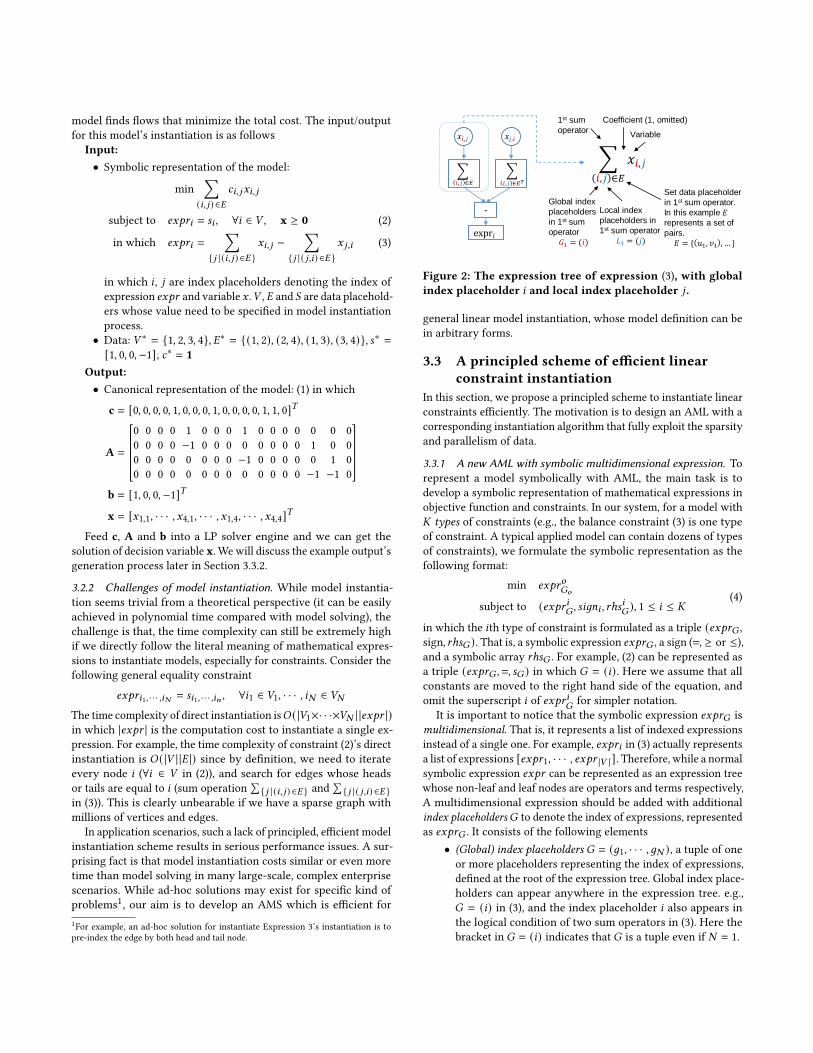
Figure 2: The expression tree of expression (3), with globalindex placeholder 𝑖 and local index placeholder 𝑗 .
general linear model instantiation, whose model definition can be
in arbitrary forms.
3.3 A principled scheme of efficient linearconstraint instantiation
In this section, we propose a principled scheme to instantiate linear
constraints efficiently. The motivation is to design an AML with a
corresponding instantiation algorithm that fully exploit the sparsity
and parallelism of data.
3.3.1 A new AML with symbolic multidimensional expression. Torepresent a model symbolically with AML, the main task is to
develop a symbolic representation of mathematical expressions in
objective function and constraints. In our system, for a model with
𝐾 types of constraints (e.g., the balance constraint (3) is one typeof constraint. A typical applied model can contain dozens of types
of constraints), we formulate the symbolic representation as the
following format:
min 𝑒𝑥𝑝𝑟𝑜𝐺𝑜
subject to (𝑒𝑥𝑝𝑟 𝑖𝐺 , 𝑠𝑖𝑔𝑛𝑖 , 𝑟ℎ𝑠𝑖𝐺 ), 1 ≤ 𝑖 ≤ 𝐾
(4)
in which the 𝑖th type of constraint is formulated as a triple (𝑒𝑥𝑝𝑟𝐺 ,sign, 𝑟ℎ𝑠𝐺 ). That is, a symbolic expression 𝑒𝑥𝑝𝑟𝐺 , a sign (=, ≥ or ≤),and a symbolic array 𝑟ℎ𝑠𝐺 . For example, (2) can be represented as
a triple (𝑒𝑥𝑝𝑟𝐺 ,=, 𝑠𝐺 ) in which 𝐺 = (𝑖). Here we assume that all
constants are moved to the right hand side of the equation, and
omit the superscript 𝑖 of 𝑒𝑥𝑝𝑟 𝑖𝐺for simpler notation.
It is important to notice that the symbolic expression 𝑒𝑥𝑝𝑟𝐺 is
multidimensional. That is, it represents a list of indexed expressionsinstead of a single one. For example, 𝑒𝑥𝑝𝑟𝑖 in (3) actually represents
a list of expressions [𝑒𝑥𝑝𝑟1, · · · , 𝑒𝑥𝑝𝑟 |𝑉 |]. Therefore, while a normal
symbolic expression 𝑒𝑥𝑝𝑟 can be represented as an expression tree
whose non-leaf and leaf nodes are operators and terms respectively,
A multidimensional expression should be added with additional
index placeholders𝐺 to denote the index of expressions, represented
as 𝑒𝑥𝑝𝑟𝐺 . It consists of the following elements
• (Global) index placeholders 𝐺 = (𝑔1, · · · , 𝑔𝑁 ), a tuple of oneor more placeholders representing the index of expressions,
defined at the root of the expression tree. Global index place-
holders can appear anywhere in the expression tree. e.g.,
𝐺 = (𝑖) in (3), and the index placeholder 𝑖 also appears in
the logical condition of two sum operators in (3). Here the
bracket in 𝐺 = (𝑖) indicates that 𝐺 is a tuple even if 𝑁 = 1.
• Operators (non-leaf nodes), receiving one or more nodes as
operands. Some specific operators such as sum (
∑) include
local index placeholders that are only valid in the scope of
these operators. E.g. the sum operator
∑{ 𝑗 | (𝑖, 𝑗) ∈𝐸 } in (3) re-
ceives 𝑥𝑖, 𝑗 as an operand, and include local index placeholder
𝑗 that is only valid in the scope of this sum operator. We will
discuss the sum operator in detail later.
• Terms (leaf nodes), a variable with its corresponding coef-
ficient. Their indices can be denoted by previously defined
global and local index placeholders. e.g. 𝑥𝑖, 𝑗 in (3) is a term
with variable 𝑥𝑖, 𝑗 and coefficient 1.
and a example is shown in the left part of Figure 2.
In this work we mainly focus on the linear constrainted scenario
that includes three operators: add (+), subtract (−) and sum (
∑).
While the add and subtract operators are trivial, we discuss the sum
operator in detail. In our formulation, we number all sum operators
in a expression, and sum operators take a fixed format: the 𝑘th sum
operator is assigned to a symbolic logical condition (𝐺𝑘 ∥𝐿𝑘 ) ∈ 𝑆𝑘 .2“∥” denotes the concatenation of tuples. For example, the 1st (𝑘 = 1)
sum operator
∑(𝑖, 𝑗) ∈𝐸 in (3) contains a logical condition (𝑖, 𝑗) ∈ 𝐸.
It consists of
• Global index placeholders 𝐺𝑘 = (𝑔𝑘1 , 𝑔𝑘2 , · · · ), a tuple whoseelements are the index placeholders from𝐺 . e.g.,𝐺1 = (𝑖) in∑(𝑖, 𝑗) ∈𝐸 .
• Local index placeholders 𝐿𝑘 = (𝑙1, 𝑙2, · · · ), which is only valid
in the scope of this sum operator. e.g., 𝐿1 = ( 𝑗) in∑(𝑖, 𝑗) ∈𝐸 .
• Data placeholder 𝑆𝑘 : A symbolic placeholder representing a
set of fixed-sized index tuples. The size of each tuple is |𝐺𝑘 | +|𝐿𝑘 |. e.g., edge set placeholder 𝐸 in
∑(𝑖, 𝑗) ∈𝐸 , representing a
set of direct edges (i.e., pair of node indices).
An example is shown in the right part of Figure 2.
3.3.2 An efficient model instantiation algorithm. To instantiate a
multidimensional expression 𝑒𝑥𝑝𝑟𝐺 given data 𝑆∗, a simple way is
to enumerate all possible combinations of global index placeholders
𝐺 (denoted as space(𝐺)), and traverse through the expression tree
for each combination to generate every single algebraic expression.
This is usually the literal meaning of mathematical expressions.
The detailed process is illustrated in Algorithm 1. For example, to
instantiate (3) with given data 𝑉 ∗ and 𝐸∗, this expression’s indexplaceholders is 𝐺 = (𝑖), and all possible values of 𝑖 are space(𝐺) ={1, 2, 3, 4}. Thenwe iterate all elements of space(𝐺). e.g., when 𝑖 = 1,
we iterate 𝐸 to generate sub-expression
∑(1, 𝑗) ∈𝐸 𝑥1, 𝑗 = 𝑥1,2 + 𝑥1,3
and
∑( 𝑗,1) ∈𝐸 𝑥 𝑗,1 = 0, then the expression will be 𝑒𝑥𝑝𝑟1 = 𝑥1,2 +
𝑥1,3. In a similar way we get 𝑒𝑥𝑝𝑟2 = 𝑥2,4 − 𝑥1,2, 𝑒𝑥𝑝𝑟3 = 𝑥3,4 −𝑥1,3, 𝑒𝑥𝑝𝑟4 = −𝑥2,4 − 𝑥3,4.
However, this approach is extremely exhaustive with time com-
plexity 𝑂 ( |space(𝐺) | |𝑆∗ |). In this section, we propose an efficient
model instantiation algorithm based on the AML proposed in pre-
vious section, whose result is identical to Algorithm 1 but with
|𝑂 (𝑆∗) | time complexity.
Lemma 3.1. For expression tree of 𝑒𝑥𝑝𝑟𝐺 , without loss of generality,we assume that every path from a leaf node to the root will go throughat least one sum operator.
2Here we simplify the denotation {𝐿𝑘 | (𝐺𝑘 ∥𝐿𝑘 ) ∈ 𝑆𝑘 } as (𝐺𝑘 ∥𝐿𝑘 ) ∈ 𝑆𝑘
Algorithm 1 Exhaustive model instantiation algorithm
Input: Symbolic multidimensional expression 𝑒𝑥𝑝𝑟𝐺 , set data 𝑆∗
Output: Constraint matrix𝐴
1: Initialize 𝐴 as an empty matrix, with number of columns equal to number of
variables.
2: for𝐺∗ ∈ space(𝐺) do3: Generate 𝑒𝑥𝑝𝑟 ∗
𝐺by replacing symbolic index placeholders𝐺 and data place-
holder 𝑆 with concrete value𝐺∗ and 𝑆∗ respectively in all nodes of 𝑒𝑥𝑝𝑟𝐺4: Do an in-order traversal to 𝑒𝑥𝑝𝑟 ∗
𝐺to generate the algebraic expression. When
visiting the 𝑖th sum operator, traverse through corresponding set data 𝑆∗𝑖 in its
logical condition.
5: Add one row to𝐴 with the generated expression.
6: end for7: return𝐴
Proof. For the leaf node whose path to the root does not include
any sum operator, we can insert a “dummy” sum operator
∑𝐺 ∈𝑆𝑖
before the node with set data 𝑆∗𝑖= space(𝐺). This operator does
not contain any local index placeholders so will not change the
result of Algorithm 1. □
Lemma 3.2. Let 𝐼 (𝑛𝑜𝑑𝑒) = {𝑖 |𝑖th sum operator is on the path fromnode to root}. Without loss of generality, we assume that for everyleaf node of the expression tree, {𝑔|𝑔 ∈ 𝐺 𝑗 , 𝑗 ∈ 𝐼 (𝑛𝑜𝑑𝑒)} = 𝐺 .
Proof. From Lemma 3.1 we know that 𝐼 (𝑛𝑜𝑑𝑒) ≠ ∅. If ∃𝑔′ ∈ 𝐺so that 𝑔′ ∉ {𝑔|𝑔 ∈ 𝐺 𝑗 , 𝑗 ∈ 𝐼 (𝑛𝑜𝑑𝑒)}, we select one sum operator∑(𝐺𝑖 ∥𝐿𝑖 ) ∈𝑆𝑖 on 𝐼 (𝑛𝑜𝑑𝑒) and expand𝐺𝑖 to𝐺𝑖 ∥𝑔′. For set data 𝑆∗𝑖 , we
replace each tuple data (𝑔∗𝑖1, · · · , 𝑔∗
𝑖𝑁, 𝑙∗𝑖1, · · · ) to a set of expanded
tuple {(𝑔∗𝑖1, · · · , 𝑔∗
𝑖𝑁, 𝑔∗
𝑗, 𝑙∗𝑖1, · · · ) |𝑔∗
𝑗∈ space(𝑔 𝑗 )}. In this way we
enumerate all possible value of 𝑔 𝑗 for every tuple data in 𝑆∗𝑖, so will
not change the result of Algorithm 1. □
With Lemma 3.1 and Lemma 3.2, we propose a model instantia-
tion algorithm. Different from Algorithm 1 that fixes the value of
all global index placeholders and traverses the expression tree for
|space(𝐺) | times, this algorithm traverses the expression tree only
once, and records the corresponding value of index placeholders
dynamically as “context information” when traverse through con-
crete set data 𝑆∗𝑖of 𝑖th sum operator. When the leaf node (term)
is reached, all the index placeholders in the term is replaced by
the actual value recorded in the context information. Meanwhile,
the actual value of all global index placeholders 𝐺 in the context is
snapshotted and attached to the index-replaced term. When the tra-
verse process is finished, we aggregate terms with the same global
index. The detailed algorithm is shown in Algorithm 2.
For example, to instantiate (3), we traverse the expression tree of
(3) in Figure 2. When we arrive at the first sum operation
∑(𝑖, 𝑗) ∈𝐸 ,
we iterate the value (𝑖, 𝑗) ∈ 𝐸 and record the context information
(e.g., record 𝑖 = 1, 𝑗 = 2 for the first edge). When we reach the leaf
node 𝑥𝑖, 𝑗 , we replace the index placeholder with the correspond-
ing value recorded in context information (e.g., we get 𝑥1,2), and
attach the actual value of all global index placeholders to the term
(e.g., attach 𝑖 = 1 to 𝑥1,2, represented as (1, 𝑥1,2)). When we finish
the traverse process, we will get (1, 𝑥1,2), (2, 𝑥2,4), (1, 𝑥1,3), (3, 𝑥3,4),(2,−𝑥1,2), (4,−𝑥2,4), (3,−𝑥1,3), (4,−𝑥3,4). By aggregating termswith
the same global index, we will get the same result as Algorithm 1.
Proposition 3.1. The outputs of Algorithm 1 and Algorithm 2are identical given the same input.
Algorithm 2 Efficient model instantiation algorithm
Input: Symbolic multidimensional expression 𝑒𝑥𝑝𝑟𝐺 , set data 𝑆∗
Output: Constraint matrix𝐴
1: procedure Replace(node, context) // node is a leaf node (term)
2: Replace the index placeholders of coefficient and variables with concrete values
in context, and return the replaced term
3: end procedure4: procedure Replace(𝐺 , context) // G is a tuple of placeholders
5: Replace the global index placeholders in𝐺 with concrete values in context,
and return
6: end procedure7: procedure Iterate(node, context)8: if node is a leaf node then9: terms← (Replace(node, context), Replace(𝐺 , context))
10: else if node is the 𝑖th sum operator then11: terms← emply list
12: Retrieve the concrete data 𝑆∗𝑖 of the 𝑖th sum operator from 𝑆∗
13: Filter all (𝑔∗1, · · · , 𝑔∗
𝑁) ∈ 𝑆∗𝑖 with the condition that 𝑔∗𝑗 = context(𝑔𝑗 ) if
𝑔𝑗 appears in the mapping key of the context
14: for (𝐺∗𝑖 , 𝐿∗𝑖 ) ∈ 𝑆∗𝑖 do15: context’← AddMapping(context,𝐺𝑖 → 𝐺∗𝑖 , 𝐿𝑖 → 𝐿∗𝑖 )16: terms← terms ∥ Iterate(child, context’)17: end for18: else if node is an add operator then19: terms← Iterate(left, context) ∥ Iterate(right, context)20: else if node is a sub operator then21: terms← Iterate(left, context) ∥ −Iterate(right, context)22: end if23: return terms
24: end procedure25: Initialize𝐴 as an empty matrix sized |𝑐𝑜𝑛𝑠𝑡𝑟𝑎𝑖𝑛𝑡𝑠 | × |𝑣𝑎𝑟𝑖𝑎𝑏𝑙𝑒𝑠 |.26: Initialize context as an empty mapping from symbolic index placeholder to con-
crete value.
27: terms← Iterate(root node of 𝑒𝑥𝑝𝑟𝐺 , context)
28: for (term,𝐺∗) ∈terms do29: Map𝐺∗ and variable to matrix index 𝑟𝑜𝑤 and 𝑐𝑜𝑙
30: 𝐴 [𝑟𝑜𝑤, 𝑐𝑜𝑙 ] = coefficient of variable
31: end for32: return𝐴
Proof. To simplify the demonstration we omit the coefficient
in all terms, which can be treated similarly to the variables.
⇒: In Algorithm 1, assume there is a variable 𝑥𝐺∗𝑥 ,𝐿∗𝑥in ex-
pression 𝑒𝑥𝑝𝑟𝐺∗ , from Lemma 3.2 we know that the union of all
𝐺𝑖 in 𝐼 (𝑥𝐺∗𝑥 ,𝐿∗𝑥 ) equals to 𝐺 . Without loss of generality we let
𝐼 (𝑥𝐺∗𝑥 ,𝐿∗𝑥 ) = 1, · · · , 𝑀 , then follow the depth-first iteration of Algo-
rithm 1, we can find a sequence (𝐺∗1∥𝐿∗
1∈ 𝑆∗
1, · · · ,𝐺∗
𝑀∥𝐿∗
𝑀∈ 𝑆∗
𝑀)
so that
⋃𝑀𝑖=1𝐺𝑖 = 𝐺 and
⋃𝑀𝑖=1𝐺
∗𝑖= 𝐺∗. For Algorithm 2, we can
follow the same sequence in the depth-first iteration and accumu-
late the mapping 𝐺𝑖 → 𝐺∗𝑖, 𝐿𝑖 → 𝐿∗
𝑖in context. Therefore when
the leaf node is finally reached, the context will contain𝐺 → 𝐺∗,then by the Replace procedure we get variable 𝑥𝐺∗𝑥 ,𝐿
∗𝑥in expression
𝑒𝑥𝑝𝑟𝐺∗ in Algorithm 2.
⇐: In Algorithm 2 assume there is a variable 𝑥𝐺∗𝑥 ,𝐿∗𝑥in expres-
sion 𝑒𝑥𝑝𝑟𝐺∗ , the context information stores mapping 𝐺 → 𝐺∗
when Iterate reached the leaf node, then following Lemma 3.2
we also have a sequence (𝐺∗1∥𝐿∗
1∈ 𝑆∗
1, · · · ,𝐺∗
𝑀∥𝐿∗
𝑀∈ 𝑆∗
𝑀) so that⋃𝑀
𝑖=1𝐺𝑖 = 𝐺 and
⋃𝑀𝑖=1𝐺
∗𝑖= 𝐺∗. Thus when 𝑒𝑥𝑝𝑟𝐺 is fixed into
𝑒𝑥𝑝𝑟𝐺∗ in Algorithm 1, we can follow the same sequence and get
variable 𝑥𝐺∗𝑥 ,𝐿∗𝑥in expression 𝑒𝑥𝑝𝑟𝐺∗ . □
3.3.3 Parallelization of the model instantiation algorithm. While
Algorithm 1 is extremely exhaustive, it is easy to be paralleled by
simply letting each worker instantiate a partition of concrete index
set space(𝐺). In this section we show that Algorithm 2 can also be
fully paralleled by transiting index partition to data partition.
g1 g2 g3
(0, 0, 1)(0, 0, 3)(0, 1, 2)(0, 2, 4)(1, 0, 0)(1, 1, 1)(2, 1, 2)(2, 2, 0)
(0, 0, 1)(0, 0, 3)(1, 0, 0)
(0, 1, 2)(1, 1, 1)(2, 1, 2)
(0, 2, 4)(2, 2, 0)
Data partition along index g2
P1={0}, P2={1}, P3={2}
S*
S1*
S2*
S3*
Figure 3: An example of data partition.
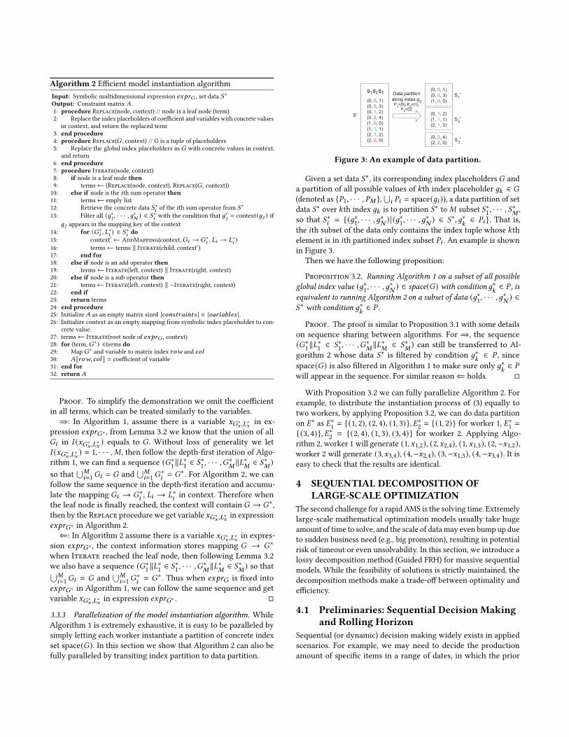
Given a set data 𝑆∗, its corresponding index placeholders 𝐺 and
a partition of all possible values of 𝑘th index placeholder 𝑔𝑘 ∈ 𝐺(denoted as {𝑃1, · · · , 𝑃𝑀 },
⋃𝑖 𝑃𝑖 = space(𝑔𝑖 )), a data partition of set
data 𝑆∗ over 𝑘th index 𝑔𝑘 is to partition 𝑆∗ to𝑀 subset 𝑆∗1, · · · , 𝑆∗
𝑀,
so that 𝑆∗𝑖= {(𝑔∗
1, · · · , 𝑔∗
𝑁) | (𝑔∗
1, · · · , 𝑔∗
𝑁) ∈ 𝑆∗, 𝑔∗
𝑘∈ 𝑃𝑖 }. That is,
the 𝑖th subset of the data only contains the index tuple whose 𝑘th
element is in 𝑖th partitioned index subset 𝑃𝑖 . An example is shown
in Figure 3.
Then we have the following proposition:
Proposition 3.2. Running Algorithm 1 on a subset of all possibleglobal index value (𝑔∗
1, · · · , 𝑔∗
𝑁) ∈ space(𝐺) with condition 𝑔∗
𝑘∈ 𝑃 , is
equivalent to running Algorithm 2 on a subset of data (𝑔∗1, · · · , 𝑔∗
𝑁) ∈
𝑆∗ with condition 𝑔∗𝑘∈ 𝑃 .
Proof. The proof is similar to Proposition 3.1 with some details
on sequence sharing between algorithms. For ⇒, the sequence
(𝐺∗1∥𝐿∗
1∈ 𝑆∗
1, · · · ,𝐺∗
𝑀∥𝐿∗
𝑀∈ 𝑆∗
𝑀) can still be transferred to Al-
gorithm 2 whose data 𝑆∗ is filtered by condition 𝑔∗𝑘∈ 𝑃 , since
space(𝐺) is also filtered in Algorithm 1 to make sure only 𝑔∗𝑘∈ 𝑃
will appear in the sequence. For similar reason⇐ holds. □
With Proposition 3.2 we can fully parallelize Algorithm 2. For
example, to distribute the instantiation process of (3) equally to
two workers, by applying Proposition 3.2, we can do data partition
on 𝐸∗ as 𝐸∗1= {(1, 2), (2, 4), (1, 3)}, 𝐸∗
2= {(1, 2)} for worker 1, 𝐸∗
1=
{(3, 4)}, 𝐸∗2= {(2, 4), (1, 3), (3, 4)} for worker 2. Applying Algo-
rithm 2, worker 1 will generate (1, 𝑥1,2), (2, 𝑥2,4), (1, 𝑥1,3), (2,−𝑥1,2),worker 2 will generate (3, 𝑥3,4), (4,−𝑥2,4), (3,−𝑥1,3), (4,−𝑥3,4). It iseasy to check that the results are identical.
4 SEQUENTIAL DECOMPOSITION OFLARGE-SCALE OPTIMIZATION
The second challenge for a rapid AMS is the solving time. Extremely
large-scale mathematical optimization models usually take huge
amount of time to solve, and the scale of data may even bump up due
to sudden business need (e.g., big promotion), resulting in potential
risk of timeout or even unsolvability. In this section, we introduce a
lossy decomposition method (Guided FRH) for massive sequential
models. While the feasibility of solutions is strictly maintained, the
decomposition methods make a trade-off between optimality and
efficiency.
4.1 Preliminaries: Sequential Decision Makingand Rolling Horizon
Sequential (or dynamic) decision making widely exists in applied
scenarios. For example, we may need to decide the production
amount of specific items in a range of dates, in which the prior
decisions will influence successive ones. More formally, for a se-
quential model of linear constraints with 𝑇 periods, its decision
variables x can be divided into 𝑇 row vectors x1, · · · , x𝑇 , so that
the constraints can be formulated as
A1x𝑇1 = b1
A2 [x1, x2]𝑇 = b2· · ·
A𝑇 [x1, x2, · · · , x𝑇 ]𝑇 = b𝑇
which indicates that the constraint matrix has a block triangular
structure. Here we assume the decision variables share the same
semantic meaning in each period, and use 𝑥𝑖𝑡 to denote the 𝑖th
variable in period 𝑡 . We refer to [4] for a detailed introduction.
To make sequential decisions in a dynamic environment, a com-
mon business practice is rolling horizon (RH)[19]. That is, we do
planning in a relatively long time window (planning horizon) us-
ing the latest available information, and only accept the generated
decisions in the first several time steps (re-planning periodicity).
When the re-planning periodicity passed, we start a new planning
horizon with updated environment information, and repeat the
above procedure.
From this perspective, compared with the decision in the re-
planning periodicity that will be actually applied, the planning
after the re-planning periodicity is more likely a “simulation-based
guidance” to reach the global optimum. That is, although the deci-
sions after the re-planning periodicity is never actually executed,
we assume that they will be executed on a simulation basis, so that
the global optimum in a longer range is considered.
In our large-scale scenario, the size of the planning horizon is
limited due to the scalability of solver engines. To enlarge the range
of future information involved in the optimization and reach global
optimum in a longer time window, we adopt the idea of “guid-
ance” in rolling horizon, but with a more computational efficient
approach.
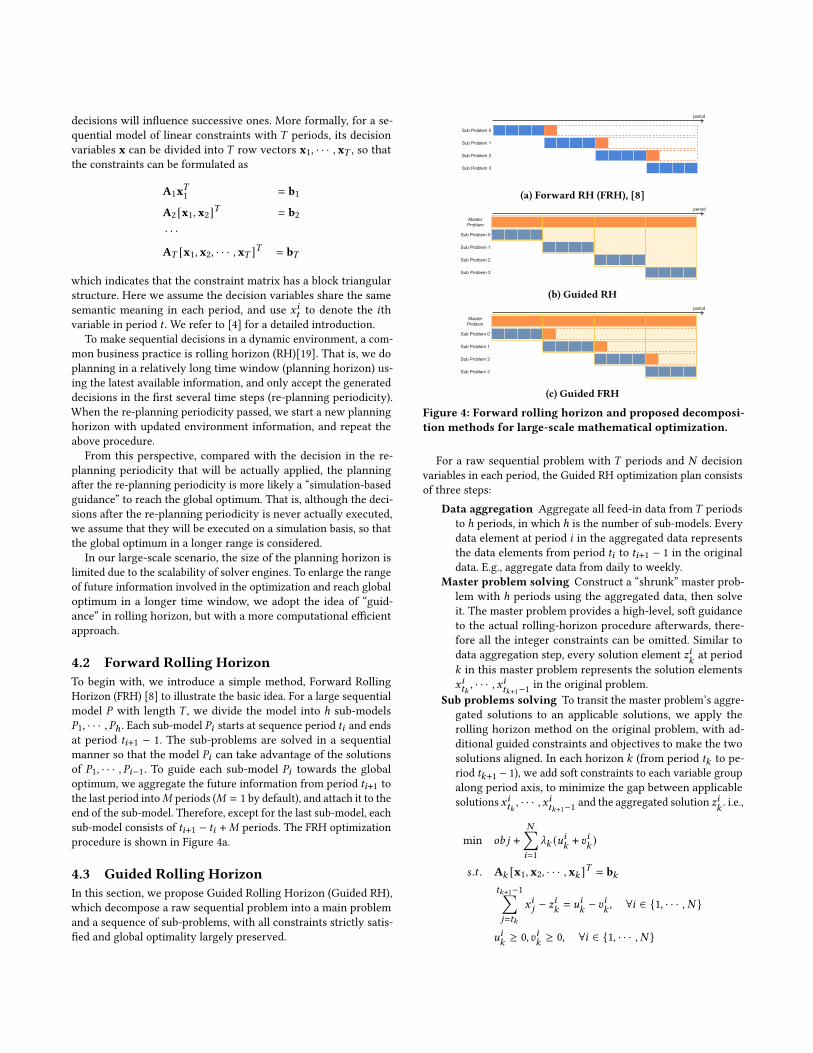
4.2 Forward Rolling HorizonTo begin with, we introduce a simple method, Forward Rolling
Horizon (FRH) [8] to illustrate the basic idea. For a large sequential
model 𝑃 with length 𝑇 , we divide the model into ℎ sub-models
𝑃1, · · · , 𝑃ℎ . Each sub-model 𝑃𝑖 starts at sequence period 𝑡𝑖 and ends
at period 𝑡𝑖+1 − 1. The sub-problems are solved in a sequential
manner so that the model 𝑃𝑖 can take advantage of the solutions
of 𝑃1, · · · , 𝑃𝑖−1. To guide each sub-model 𝑃𝑖 towards the global
optimum, we aggregate the future information from period 𝑡𝑖+1 tothe last period into𝑀 periods (𝑀 = 1 by default), and attach it to the
end of the sub-model. Therefore, except for the last sub-model, each
sub-model consists of 𝑡𝑖+1 − 𝑡𝑖 +𝑀 periods. The FRH optimization
procedure is shown in Figure 4a.
4.3 Guided Rolling HorizonIn this section, we propose Guided Rolling Horizon (Guided RH),
which decompose a raw sequential problem into a main problem
and a sequence of sub-problems, with all constraints strictly satis-
fied and global optimality largely preserved.
period
Sub Problem 0
Sub Problem 1
Sub Problem 2
Sub Problem 3
(a) Forward RH (FRH), [8]period
Master Problem
Sub Problem 0
Sub Problem 1
Sub Problem 2
Sub Problem 3
(b) Guided RHperiod
Master Problem
Sub Problem 0
Sub Problem 1
Sub Problem 2
Sub Problem 3
(c) Guided FRH
Figure 4: Forward rolling horizon and proposed decomposi-tion methods for large-scale mathematical optimization.
For a raw sequential problem with 𝑇 periods and 𝑁 decision
variables in each period, the Guided RH optimization plan consists
of three steps:
Data aggregation Aggregate all feed-in data from 𝑇 periods
to ℎ periods, in which ℎ is the number of sub-models. Every
data element at period 𝑖 in the aggregated data represents
the data elements from period 𝑡𝑖 to 𝑡𝑖+1 − 1 in the original
data. E.g., aggregate data from daily to weekly.
Master problem solving Construct a “shrunk” master prob-
lem with ℎ periods using the aggregated data, then solve
it. The master problem provides a high-level, soft guidance
to the actual rolling-horizon procedure afterwards, there-
fore all the integer constraints can be omitted. Similar to
data aggregation step, every solution element 𝑧𝑖𝑘at period
𝑘 in this master problem represents the solution elements
𝑥𝑖𝑡𝑘, · · · , 𝑥𝑖
𝑡𝑘+1−1 in the original problem.
Sub problems solving To transit the master problem’s aggre-
gated solutions to an applicable solutions, we apply the
rolling horizon method on the original problem, with ad-
ditional guided constraints and objectives to make the two
solutions aligned. In each horizon 𝑘 (from period 𝑡𝑘 to pe-
riod 𝑡𝑘+1 − 1), we add soft constraints to each variable group
along period axis, to minimize the gap between applicable
solutions 𝑥𝑖𝑡𝑘, · · · , 𝑥𝑖
𝑡𝑘+1−1 and the aggregated solution 𝑧𝑖𝑘. i.e.,
min 𝑜𝑏 𝑗 +𝑁∑𝑖=1
_𝑘 (𝑢𝑖𝑘 + 𝑣𝑖𝑘)
𝑠 .𝑡 . A𝑘 [x1, x2, · · · , x𝑘 ]𝑇 = b𝑘𝑡𝑘+1−1∑𝑗=𝑡𝑘
𝑥𝑖𝑗 − 𝑧𝑖𝑘= 𝑢𝑖
𝑘− 𝑣𝑖
𝑘, ∀𝑖 ∈ {1, · · · , 𝑁 }
𝑢𝑖𝑘≥ 0, 𝑣𝑖
𝑘≥ 0, ∀𝑖 ∈ {1, · · · , 𝑁 }
period
x
y
z
……
state variable
fixed variablesfree variables
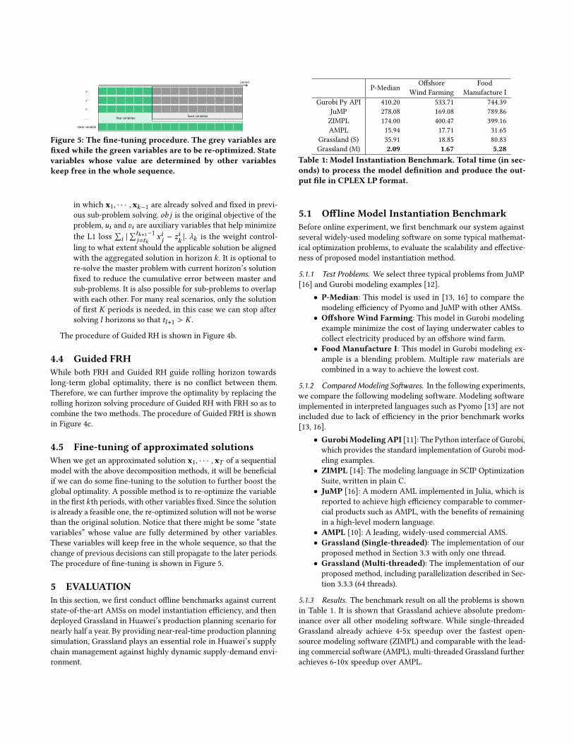
Figure 5: The fine-tuning procedure. The grey variables arefixed while the green variables are to be re-optimized. Statevariables whose value are determined by other variableskeep free in the whole sequence.
in which x1, · · · , x𝑘−1 are already solved and fixed in previ-
ous sub-problem solving. 𝑜𝑏 𝑗 is the original objective of the
problem, 𝑢𝑖 and 𝑣𝑖 are auxiliary variables that help minimize
the L1 loss
∑𝑖 |∑𝑡𝑘+1−1
𝑗=𝑡𝑘𝑥𝑖𝑗− 𝑧𝑖
𝑘|. _𝑘 is the weight control-
ling to what extent should the applicable solution be aligned
with the aggregated solution in horizon 𝑘 . It is optional to
re-solve the master problem with current horizon’s solution
fixed to reduce the cumulative error between master and
sub-problems. It is also possible for sub-problems to overlap
with each other. For many real scenarios, only the solution
of first 𝐾 periods is needed, in this case we can stop after
solving 𝑙 horizons so that 𝑡𝑙+1 > 𝐾 .
The procedure of Guided RH is shown in Figure 4b.
4.4 Guided FRHWhile both FRH and Guided RH guide rolling horizon towards
long-term global optimality, there is no conflict between them.
Therefore, we can further improve the optimality by replacing the
rolling horizon solving procedure of Guided RH with FRH so as to
combine the two methods. The procedure of Guided FRH is shown
in Figure 4c.
4.5 Fine-tuning of approximated solutionsWhen we get an approximated solution x1, · · · , x𝑇 of a sequential
model with the above decomposition methods, it will be beneficial
if we can do some fine-tuning to the solution to further boost the
global optimality. A possible method is to re-optimize the variable
in the first 𝑘th periods, with other variables fixed. Since the solution
is already a feasible one, the re-optimized solution will not be worse
than the original solution. Notice that there might be some “state
variables” whose value are fully determined by other variables.
These variables will keep free in the whole sequence, so that the
change of previous decisions can still propagate to the later periods.
The procedure of fine-tuning is shown in Figure 5.
5 EVALUATIONIn this section, we first conduct offline benchmarks against current
state-of-the-art AMSs on model instantiation efficiency, and then
deployed Grassland in Huawei’s production planning scenario for
nearly half a year. By providing near-real-time production planning
simulation, Grassland plays an essential role in Huawei’s supply
chain management against highly dynamic supply-demand envi-
ronment.
P-Median
Offshore
Wind Farming
Food
Manufacture I
Gurobi Py API 410.20 533.71 744.39
JuMP 278.08 169.08 789.86
ZIMPL 174.00 400.47 399.16
AMPL 15.94 17.71 31.65
Grassland (S) 35.91 18.85 80.83
Grassland (M) 2.09 1.67 5.28Table 1: Model Instantiation Benchmark. Total time (in sec-onds) to process the model definition and produce the out-put file in CPLEX LP format.
5.1 Offline Model Instantiation BenchmarkBefore online experiment, we first benchmark our system against
several widely-used modeling software on some typical mathemat-
ical optimization problems, to evaluate the scalability and effective-
ness of proposed model instantiation method.
5.1.1 Test Problems. We select three typical problems from JuMP
[16] and Gurobi modeling examples [12].
• P-Median: This model is used in [13, 16] to compare the
modeling efficiency of Pyomo and JuMP with other AMSs.
• Offshore Wind Farming: This model in Gurobi modeling
example minimize the cost of laying underwater cables to
collect electricity produced by an offshore wind farm.
• Food Manufacture I: This model in Gurobi modeling ex-
ample is a blending problem. Multiple raw materials are
combined in a way to achieve the lowest cost.
5.1.2 Compared Modeling Softwares. In the following experiments,
we compare the following modeling software. Modeling software
implemented in interpreted languages such as Pyomo [13] are not
included due to lack of efficiency in the prior benchmark works
[13, 16].
• GurobiModelingAPI [11]: The Python interface of Gurobi,which provides the standard implementation of Gurobi mod-
eling examples.
• ZIMPL [14]: The modeling language in SCIP Optimization
Suite, written in plain C.
• JuMP [16]: A modern AML implemented in Julia, which is
reported to achieve high efficiency comparable to commer-
cial products such as AMPL, with the benefits of remaining
in a high-level modern language.
• AMPL [10]: A leading, widely-used commercial AMS.
• Grassland (Single-threaded): The implementation of our
proposed method in Section 3.3 with only one thread.
• Grassland (Multi-threaded): The implementation of our
proposed method, including parallelization described in Sec-
tion 3.3.3 (64 threads).
5.1.3 Results. The benchmark result on all the problems is shown
in Table 1. It is shown that Grassland achieve absolute predom-
inance over all other modeling software. While single-threaded
Grassland already achieve 4-5x speedup over the fastest open-
source modeling software (ZIMPL) and comparable with the lead-
ing commercial software (AMPL), multi-threaded Grassland further
achieves 6-10x speedup over AMPL.

105
106
107
10−1
100
101
102
103
104
Number of Constraints
TimeCost(s)
Gurobi API
JuMP
ZIMPL
AMPL
Grassland (S)
Grassland (M)
(a)
104
105
106
107
10−2
10−1
100
101
102
103
104
Number of Constraints
TimeCost(s)
Gurobi API
JuMP
ZIMPL
AMPL
Grassland (S)
Grassland (M)
(b)
104
105
106
107
10−1
100
101
102
103
104
Number of Constraints
TimeCost(s)
Gurobi API
JuMP
ZIMPL
AMPL
Grassland (S)
Grassland (M)
(c)
Figure 6: Offline model instantiation benchmark on (a) P-Median (b) Offshore Wind Farming (c) Food Manufacture I.
Baseline RH FRH G-RH G-FRH
0
500
1,000
1,500
2,000
2,500
3,000
3,500
4,000
Methods
TimeCost(s)
Instantiation time
Solving time
Objective value
Optimal obj
5.1
5.2
5.3
5.4
5.5
5.6
·109
5.156 · 109
5.540 · 109(+7.45%)
5.198 · 109(+0.81%)
5.265 · 109(+2.11%)
5.175 · 109(+0.36%)
ObjectiveValue
(a)
Baseline RH FRH G-RH G-FRH
0
500
1,000
1,500
2,000
2,500
3,000
3,500
4,000
Methods
TimeCost(s)
Instantiation time
Solving time
Objective value
Optimal obj
5.1
5.2
5.3
5.4
5.5
5.6
·109
5.156 · 109
5.338 · 109(+3.52%)
5.197 · 109(+0.78%)
5.221 · 109(+1.26%)
5.173 · 109(+0.33%)
ObjectiveValue
(b)
01 · 106 2 · 106 3 · 106 4 · 106
100
101
102
103
104
Number of Constraints
TimeCost(s)
ZIMPL based version
Gurobi API based version
Grassland (S)
Grassland (M)
(c)
Figure 7: Online experiment results. (a) Comparison between baseline and different decomposition methods on time cost andoptimality. (b) Same as (a) with fine-tuning of first 20 periods. (c) Comparison of model instantiation efficiency.
We also tested the software on different scales of models. The
result is shown in Figure 6. It is shown that Grassland has superior
performance over all scale of models.
5.2 Online Experiment5.2.1 Background: Production planning and supply-demand analy-sis. Production planning is the planning of production activities to
transform raw materials (supply) into finished products, meeting
customer’s order (demand) in the most efficient or economical way
possible. It lies in the core of manufacturing companies’ supply
chain management, directly influencing the profit and customer
satisfaction. Mathematical optimization is a mainstream method for
production planning, and [18] provides a comprehensive introduc-
tion to this. As a world-leading electronic manufacturer, Huawei
provides more than ten thousand kinds of end products, with even
much more kinds of raw materials and intermediate assemblies,
to satisfy millions of demands from all over the world. Modeling
in such a large-scale scenario involves millions of variables and
constraints.
While mathematical optimization can deliver near-optimal pro-
duction planning solution for a certain input of supply and demand,
The demand and supply itself is always changing with high uncer-
tainty due to external dynamic factors. Our planning department
needs to react quickly to such changes to ensure business continu-
ity, which is called supply-demand analysis. To support the analysis,a crucial process is production planning simulation which returns
the final planning result (e.g., fulfillment rate) for a certain input of
supply and demand, helping planners evaluate and improve their
analysis. For example, when several raw materials are suddenly
unavailable, planners may try different ways to increase the supply
of alternative materials and run production planning simulation for
each of them, adjust the supply iteratively to increase the fulfillment
rate of related end products, and get the final supply adjustment
decision.
5.2.2 Dataset and Compared Methods. The dataset is from real pro-
duction environment which consists of all needed manufacturing
data in 78 weeks (one week per period). The instantiated model
consists of 5,957,634 variables, 3,443,465 constraints and 30,366,971
nonzero elements in the constraint matrix. In the following ex-
periments, we compare the result before and after the application
of Grassland in the production planning simulation scenario. The
baseline is the original method before the deployment of Grassland,
which is quite standard: ZIMPL is used for modeling and instantia-
tion, and the instantiated full model is directly solved without any
decomposition. The decomposition methods in section 4 (RH, FRH,
Guided RH, Guided FRH) are tested separately. Sequence length
𝑇 = 78, number of submodels ℎ = 8, fine-tuning periods 𝑘 = 20. All
models are solved via Mosek ApS[3].3
5.2.3 Results. The main result is shown in Figure 7a. Our proposed
methods can achieve significant acceleration (15-35x faster) than
baseline method, while the feasibility is strictly maintained and
3Note that we cannot deploy more efficient solvers like CPLEX on Huawei’s online
enterprise environment due to export restriction of the US (so as advanced AMSs like
AMPL). However, all solvers always deliver exact optimal solution if possible, and
have similar exponential curves between problem scale and solving time. Therefore
the selection of external solvers will not change the optimality and solving time ratio.

the loss of objective is small. For Guided FRH, it can achieve 15x
acceleration with only 0.36% of the objective loss. Practically, such
a tiny optimality loss does not cause sensible issues (0.1% ∼ 0.2%
fluctuation of fulfillment ratio), especially considering that multiple
source of more dominant error exist in complex business models
such as prediction and approximation error.
The fine-tuning result is shown in Figure 7b in which the first 20
periods of the problem is re-optimized following Section 4.5. It is
shown that fine-tuning can significantly narrow the gap between
the objective value of decomposition methods and the optimal one.
Additionally, for instantiation efficiency in online scenarios, we
compare Grassland with two legacy systems that we previously de-
veloped and deployed in online environment, based on ZIMPL and
Gurobi Modeling API respectively. We use the number of periods
involved to control the model size. The result is shown in Figure 7c.
It is shown that the result is aligned with offline benchmarks in
Figure 6.
6 CONCLUSIONIn this paper, we propose Grassland, an algebraic modeling system
that is efficient in large-scale mathematical optimization scenar-
ios, including a parallelized instantiation scheme for general linear
constraints, and a lossy sequential decomposition method that ac-
celerates large-scale model solving exponentially. We perform both
offline benchmarks and online deployment in Huawei’s produc-
tion planning scenario. The results demonstrate the significant
superiority of Grassland over strong baselines.
APPENDIXA IMPLEMENTATION DETAILSAs an algebraic modeling system, Grassland is implemented in five
layers:
Modeling API (AML) The grassland modeling API is imple-
mented as a Python package grassland (gl).Intermediate representation (IR) layer This layer plays as
a bridge between Modeling API and highly-efficient c++
backend. Models defined by Grassland modeling API is trans-
lated into a unified, JSON-based intermediate representation
with six components (variables, constants, index placehold-
ers, expression graphs, constraints and bounds).
Decomposition layer Implements four decomposition meth-
ods in section 4 (RH, FRH, Guided RH, Guided FRH).
Model instantiation layer Implements the parallelizedmodel
instantiation scheme in Section 3.3.2 and Section 3.3.3. The
parallelization is implemented by multi-threaded program-
ming. Due to the extreme efficiency of our proposed method,
even the float-to-string conversion becomes a significant bot-
tleneck. Here we apply Ryu [2] to accelerate the conversion.
Solver layer Calls different solver engine to solve the instan-
tiated model or sub-model and return back the solution.
B INTEGRATIONWITH ROUNDINGPROCEDURE
In applied optimization pipeline, there usually exist some integer
constraints for decision variables. To achieve this, a mixed integer
Test Problem #(variables) #(constraints) #(nonzeros)
P-Median 5,050,000 5,000,164 15,050,000
Offshore Wind Farming 4,170,120 4,220,120 10,425,300
Food Manufacture I 5,006,394 14,974,502 39,932,750
Table 2: The basic statistics of the benchmark test problemsin Table 1.
programming model or an external heuristics rounding procedure
may apply. However, the efficiency of rounding procedure can
heavily rely on the scale of the model, as well as the number of
integer constraints. With the above decomposition methods, we can
round the variables at the same time when we solve each sub-model.
Since the sub-model is significantly smaller than the original one,
the rounding procedure will also be largely accelerated.
C TEST PROBLEMS FOR MODELINSTANTIATION
The basic statistics of the benchmark test problems in Table 1 is
listed in Table 2. Problem data is randomly generated while main-
taining the feasibility, and we control the size of the data to generate
different scale of models in Figure 6.
D EXPREIMENTAL SETTINGFor offline model instantiation benchmark, all benchmarks are run
on a server with 32-core (64-thread) CPUs and 192GB memory.
The output format of all constructed problems is set to CPLEX LP
format (a standard LP/MIP format that is supported by most of
the mathematical solvers). The identity of all constructed problems
by different softwares on small and medium size are checked by
actual solving with Gurobi with the same optimized objective value,
and checked by static comparison script for extremely large size
that cannot be directly solved in reasonable time. MIP problems are
relaxed into LP in the identity checking process to extend scalability.
For multi-threaded Grassland, the size of thread pool is set to 64.
The basic information of the benchmark problems are shown in
Table 2.
For online experiment. all experiments are run on a Huawei
cloud server with 32-core (64-thread) CPUs and 256GB memory.
All models are solved via Mosek ApS[3]. For production planning
problem, the sequence length 𝑇 = 78 and we use number of sub-
models ℎ = 8, fine-tuning periods 𝑘 = 20 for all decomposition
methods.
Software version:
• Gurobi Modeling API (7.5.1, released in Jul 2017)4
• ZIMPL (3.4.0, released in June 2020)
• JuMP (0.21.3, released in June 2020)
• AMPL (20200810, released in Aug 2020)
E EXPERIMENTAL RESULTThe detailed result of online experiment is shown in Table 3 and
Table 4.
4Due to export restrictions, we cannot purchase and deploy the latest version of Gurobi
in Huawei’s enterprise environment.

Method
Model
instantiation time
Solving
time
Total
time
Objective
(×109)Baseline 857.00 3135.16 3992.16 5.15626
RH 4.94 40.80 45.74 (+7.45%) 5.54017
FARH 8.54∗ + 6.78 67.68 83.00 (+0.81%) 5.19818
G-RH 28.84∗∗ + 8.79∗ + 6.20 73.31 117.14 (+2.11%) 5.26513
G-FARH 30.99∗∗ + 11.07∗ + 7.43 167.62 217.11 (+0.36%) 5.17477Table 3: Sequential decomposition benchmark on demand-supply analysis problem. In “Model instantiation time” col-umn, timemarked with “*” is the time for data compression,time marked with “**” is the time to generate guided con-straints and objectives.
Method
Model
instantiation time
Solving
time
Total
time
Objective
(×109)Baseline 857.00 3135.16 3992.16 5.15626
RH 8.16 150.35† + 40.80 199.31 (+3.52%) 5.33775
FARH 8.54∗ + 9.19 147.11† + 67.68 232.52 (+0.78%) 5.19651
G-RH 28.84∗∗ + 8.79∗ + 9.29 138.11† + 73.31 258.34 (+1.26%) 5.22104
G-FARH 30.99∗∗ + 11.07∗ + 9.93 116.41† + 167.62 336.02 (+0.33%) 5.17321Table 4: Fine-tuning benchmark on demand-supply analysisproblem. In “Solving time” column, timemarked with “†” isthe extra solving time for fine tuning.
F PRODUCTION PLANNING MODELWhile real-world production planning models are complex with lots
of variants for different scenarios, here we show a self-contained,
simplified version with only three types of constraints. We refer to
[18] for a detailed introduction.
min
∑𝑡,𝑝,𝑖
𝐶𝑚𝑡,𝑝,𝑖𝑚𝑡,𝑝,𝑖 +∑𝑡,𝑝,𝑖
𝐶𝑥𝑡,𝑝,𝑖𝑥𝑡,𝑝,𝑖 +∑𝑡,𝑝,𝑖
𝐶𝑝𝑢𝑟
𝑡,𝑝,𝑖𝑝𝑢𝑟𝑡,𝑝,𝑖
+∑
𝑡,𝑝,𝑖,𝑖′, 𝑗
𝐶𝑟𝑝
𝑡,𝑝,𝑖,𝑖′, 𝑗𝑟𝑝𝑡,𝑝,𝑖,𝑖′, 𝑗 +
∑𝑡,𝑝,𝑖, 𝑗
𝐶𝑟𝑡,𝑝,𝑖, 𝑗𝑟𝑡,𝑝,𝑖, 𝑗
𝑠 .𝑡 . 𝑖𝑛𝑣𝑡,𝑝,𝑖 = 𝑖𝑛𝑣𝑡−1,𝑝,𝑖 + 𝑖𝑛𝑏𝑜𝑢𝑛𝑑𝑡,𝑝,𝑖 − 𝑜𝑢𝑡𝑏𝑜𝑢𝑛𝑑𝑡,𝑝,𝑖 (5)
𝑖𝑛𝑏𝑜𝑢𝑛𝑑𝑡,𝑝,𝑖 =∑𝑡 ′𝑥𝑡 ′,𝑝,𝑖 +
∑𝑡 ′𝑝𝑢𝑟𝑡 ′,𝑝,𝑖 +
∑𝑝′𝑠𝑡,𝑝′,𝑝,𝑖
+∑𝑖′, 𝑗
𝑟𝑝𝑡,𝑝,𝑖,𝑖′, 𝑗 +∑𝑗
𝑟𝑡,𝑝,𝑗,𝑖 + 𝑃𝑂𝑡,𝑝,𝑖 +𝑊𝐼𝑃𝑡,𝑝,𝑖
𝑜𝑢𝑡𝑏𝑜𝑢𝑛𝑑𝑡,𝑝,𝑖 =∑𝑗
𝐵𝑡,𝑝,𝑖, 𝑗𝑥𝑡,𝑝,𝑗 +∑𝑝′𝑠𝑡,𝑝,𝑝′,𝑖 +
∑𝑖′, 𝑗
𝑟𝑝𝑡,𝑝,𝑖′,𝑖, 𝑗
+∑𝑗
𝑟𝑡,𝑝,𝑖, 𝑗 + 𝑧𝑡,𝑝,𝑖
for (𝑡, 𝑝, 𝑖) ∈ 𝑃𝑚𝑡,𝑝,𝑖 =𝑚𝑡−1,𝑝,𝑖 − 𝑧𝑡,𝑝,𝑖 + 𝐷𝑡,𝑝,𝑖 (6)
for (𝑡, 𝑝, 𝑖) ∈ 𝑃∑𝑖′𝑟𝑝𝑡,𝑝,𝑖,𝑖′, 𝑗 ≤ 𝐵𝑡,𝑝,𝑖, 𝑗𝑥𝑡,𝑝,𝑗 (7)
for (𝑡, 𝑝, 𝑖, 𝑗) ∈ 𝐵𝑂𝑀
Indices:
• 𝑖, 𝑖 ′, 𝑗 : items (raw material, sub-assembly or end product).
• 𝑝: plant.• 𝑡 : period.
Decision variables:
• 𝑥𝑡,𝑝,𝑖 , 𝑝𝑢𝑟𝑡,𝑝,𝑖 , 𝑧𝑡,𝑝,𝑖 : the production/purchase/deliver amount
of item 𝑖 in plant 𝑝 at period 𝑡 .
• 𝑠𝑡,𝑝,𝑝′,𝑡 : the transit amount of item 𝑖 from plant 𝑝 to plant 𝑝 ′
at period 𝑡 .
• 𝑟𝑡,𝑝,𝑖, 𝑗 : the amount that item 𝑖 replace item 𝑗 in plant 𝑝 at
period 𝑡 .
• 𝑟𝑝𝑡,𝑝,𝑖,𝑖′, 𝑗 : the amount that item 𝑖 ′ replace item 𝑖 to produce
item 𝑗 in plant 𝑝 at period 𝑡 .
State variables (whose value is determined by other decision
variables):
• 𝑖𝑛𝑣𝑡,𝑝,𝑖 : the inventory amount of item 𝑖 in plant 𝑝 at period
𝑡 .
• 𝑚𝑡,𝑝,𝑖 : the delay amount of item 𝑖 in plant 𝑝 at period 𝑡 .
All the value of decision and state variables are not less than
zero.
Some important constants (note that not all constants are listed
due to space limit. Every sum operation contains a constant that
controls the range of indices):
• 𝐶𝑚,𝐶𝑠 ,𝐶𝑝𝑢𝑟 ,𝐶𝑟𝑝 ,𝐶𝑟 : the cost of delay, transition, purchase
and replacement. (Delay cost will usually dominate the ob-
jective)
• 𝑃 [𝑡, 𝑝, 𝑖]: item 𝑖 will be produced in plant 𝑝 at period 𝑡 .
• 𝐵𝑂𝑀 [𝑡, 𝑝, 𝑖, 𝑗]: 𝑗 is the parent of 𝑖 in plant 𝑝 at period 𝑡 .
• 𝐵𝑡,𝑝,𝑖, 𝑗 : number of item 𝑖’s amount that need to be consumed
to producing one item 𝑗 .
• 𝑃𝑂𝑡,𝑝,𝑖 ,𝑊 𝐼𝑃𝑡,𝑝,𝑖 : the amount of purchase order (PO) / work-
in-progress (WIP) of item 𝑖 in plant 𝑝 at period 𝑡 .
Constraints:
• Equation 5: inventory constraint. The current inventory
amount equals to last period’s inventory plus inbound minus
outbound.
• Equation 6: delay constraint. The current delay amount
equals to last period’s delay amount plus delivery amount
minus demand amount.
• Equation 7: replacement constraint. For all component-assembly
relation, the sum of replacement amount cannot exceed the
needed amount for assembly’s production.
REFERENCES[1] Martín Abadi, Paul Barham, Jianmin Chen, Zhifeng Chen, Andy Davis, Jeffrey
Dean, Matthieu Devin, Sanjay Ghemawat, Geoffrey Irving, Michael Isard, Man-
junath Kudlur, Josh Levenberg, Rajat Monga, Sherry Moore, Derek G. Murray,
Benoit Steiner, Paul Tucker, Vijay Vasudevan, Pete Warden, Martin Wicke, Yuan
Yu, and Xiaoqiang Zheng. 2016. TensorFlow: A System for Large-Scale Ma-
chine Learning. In 12th USENIX Symposium on Operating Systems Design andImplementation (OSDI 16). USENIX Association, Savannah, GA, 265–283. https:
//www.usenix.org/conference/osdi16/technical-sessions/presentation/abadi
[2] Ulf Adams. 2018. Ryu: Fast Float-to-String Conversion. In Proceedings of the 39thACM SIGPLAN Conference on Programming Language Design and Implementation(Philadelphia, PA, USA) (PLDI 2018). Association for Computing Machinery, New
York, NY, USA, 270–282. https://doi.org/10.1145/3192366.3192369
[3] MOSEK ApS. 2019. MOSEK optimization suite.
[4] Stephen P. Bradley. 1977. Applied mathematical programming. Addison-Wesley
Pub. Co., Reading, Mass.
[5] Anthony Brook, David Kendrick, and Alexander Meeraus. 1988. GAMS, a user’s
guide. ACM Signum Newsletter 23, 3-4 (1988), 10–11.

[6] Mingyuan Chen and Weimin Wang. 1997. A linear programming model for
integrated steel production and distribution planning. International Journal ofOperations & Production Management (1997).
[7] Gerard Cornuejols and Reha Tütüncü. 2006. Optimization methods in finance.Vol. 5. Cambridge University Press.
[8] A.D. Dimitriadis, N. Shah, and C.C. Pantelides. 1997. RTN-based rolling horizon
algorithms for medium term scheduling of multipurpose plants. Computers &Chemical Engineering 21 (1997), S1061 – S1066.
[9] Rafael Epstein, Andres Neely, Andres Weintraub, Fernando Valenzuela, Sergio
Hurtado, Guillermo Gonzalez, Alex Beiza, Mauricio Naveas, Florencio Infante,
Fernando Alarcon, et al. 2012. A strategic empty container logistics optimization
in a major shipping company. Interfaces 42, 1 (2012), 5–16.[10] Robert Fourer, David M Gay, and Brian W Kernighan. 1990. A modeling language
for mathematical programming. Management Science 36, 5 (1990), 519–554.[11] Gurobi Optimization, LLC. 2018. Gurobi optimizer reference manual. https:
//www.gurobi.com/documentation/9.0/refman/index.html. (2018).
[12] Gurobi Optimization, LLC. 2019. Gurobi modeling examples. https://gurobi.
github.io/modeling-examples/.
[13] William EHart, Jean-PaulWatson, and David LWoodruff. 2011. Pyomo: modeling
and solving mathematical programs in Python. Mathematical ProgrammingComputation 3, 3 (2011), 219.
[14] Thorsten Koch. 2004. Rapid Mathematical Programming. Ph.D. Dissertation.
Technische Universität Berlin. http://www.zib.de/Publications/abstracts/ZR-04-
58/ ZIB-Report 04-58.
[15] Johan Lofberg. 2004. YALMIP: A toolbox for modeling and optimization in
MATLAB. In 2004 IEEE international conference on robotics and automation (IEEECat. No. 04CH37508). IEEE, 284–289.
[16] Miles Lubin and Iain Dunning. 2015. Computing in Operations Research Using
Julia. INFORMS Journal on Computing 27, 2 (2015), 238–248. https://doi.org/10.
1287/ijoc.2014.0623
[17] Adam Paszke, Sam Gross, Francisco Massa, Adam Lerer, James Bradbury, Gregory
Chanan, Trevor Killeen, Zeming Lin, Natalia Gimelshein, Luca Antiga, Alban Des-
maison, Andreas Kopf, Edward Yang, Zachary DeVito, Martin Raison, Alykhan
Tejani, Sasank Chilamkurthy, Benoit Steiner, Lu Fang, Junjie Bai, and Soumith
Chintala. 2019. PyTorch: An Imperative Style, High-Performance Deep Learn-
ing Library. In Advances in Neural Information Processing Systems, H. Wallach,
H. Larochelle, A. Beygelzimer, F. d'Alché-Buc, E. Fox, and R. Garnett (Eds.), Vol. 32.
Curran Associates, Inc., 8026–8037. https://proceedings.neurips.cc/paper/2019/
file/bdbca288fee7f92f2bfa9f7012727740-Paper.pdf
[18] Yves Pochet and Laurence A. Wolsey. 2010. Production Planning by Mixed IntegerProgramming (1st ed.). Springer Publishing Company, Incorporated.
[19] Suresh Sethi and Gerhard Sorger. 1991. A theory of rolling horizon decision
making. Annals of Operations Research 29, 1 (01 Dec 1991), 387–415. https:
//doi.org/10.1007/BF02283607