Graduate School ETD Form 9 (Revised 12/07)

PURDUE UNIVERSITY GRADUATE SCHOOL

Thesis/Dissertation Acceptance

This is to certify that the thesis/dissertation prepared

By

Entitled

For the degree of

Is approved by the final examining committee:

Chair

To the best of my knowledge and as understood by the student in the Research Integrity and Copyright Disclaimer (Graduate School Form 20), this thesis/dissertation adheres to the provisions of Purdue University’s “Policy on Integrity in Research” and the use of copyrighted material.

Approved by Major Professor(s): ____________________________________

____________________________________

Approved by: Head of the Graduate Program Date

Sree Likhita Gavini

CONTROL OF NON-MINIMUM PHASE POWER CONVERTERS

Master of Science in Electrical and Computer Engineering

Afshin Izadian

Lingxi Li

Maher E Rizkalla

Afshin Izadian

Lingxi Li

Brian King 04/17/2012

Graduate School Form 20 (Revised 9/10)

PURDUE UNIVERSITY GRADUATE SCHOOL

Research Integrity and Copyright Disclaimer

Title of Thesis/Dissertation:

For the degree of Choose your degree

I certify that in the preparation of this thesis, I have observed the provisions of Purdue University Executive Memorandum No. C-22, September 6, 1991, Policy on Integrity in Research.*

Further, I certify that this work is free of plagiarism and all materials appearing in this thesis/dissertation have been properly quoted and attributed.

I certify that all copyrighted material incorporated into this thesis/dissertation is in compliance with the United States’ copyright law and that I have received written permission from the copyright owners for my use of their work, which is beyond the scope of the law. I agree to indemnify and save harmless Purdue University from any and all claims that may be asserted or that may arise from any copyright violation.

______________________________________ Printed Name and Signature of Candidate

______________________________________ Date (month/day/year)

*Located at http://www.purdue.edu/policies/pages/teach_res_outreach/c_22.html

CONTROL OF NON-MINIMUM PHASE POWER CONVERTERS

Master of Science in Electrical and Computer Engineering

Sree Likhita Gavini

4/18/2012

CONTROL OF NON-MINIMUM PHASE POWER CONVERTERS

A Thesis

Submitted to the Faculty

of

Purdue University

by

Sree Likhita Gavini

In Partial Fulfillment of the

Requirements for the Degree

of

Master of Science in Electrical and Computer Engineering

May 2012

Purdue University

Indianapolis, Indiana

ii

ACKNOWLEDGEMENTS

This research would not have been possible had it not been for my advisor, Dr. Afshin

Izadian. Despite his busy schedule, Dr. Izadian took time to teach us a short course every

week on Nonlinear Controls which quickened my learning curve. The weekly meetings

and the numerous hours of discussion with Dr. Izadian further helped me move forward

in my research. With a mentor, under whose constant encouragement and support, I

found motivation and guidance to successfully complete my research.

I am also grateful to Dr. Lingxi Li, my Co-Chair, for his continual support throughout

the course of my research and to Dr. Maher Rizkalla for making time out of his busy

schedule to be on my advisory committee.

I would also like to thank Mr. Nathaniel Girrens and Mr. Heng Yang from my

research group, for helping me with the converter test bed and dSPACE rapid prototyping

device for verification of my control designs and for offering me valuable suggestions. I

also acknowledge my colleague Ms. Ayana Pusha, who always had been my source of

comfort during all my frustrations.

Finally, I thank the Departments of Electrical and Computer Engineering and

Technology for allowing joint research collaboration between the two departments and

Ms. Valerie Lim Diemer and Ms. Sherrie Tucker for assisting me throughout my

Master’s program. Last, but not the least, I am obliged to my family and friends for their

staunch patronage during the two years of my Master’s program.

iii

TABLE OF CONTENTS

Page

LIST OF FIGURES .............................................................................................................v

ABSTRACT ...................................................................................................................... vii

1. INTRODUCTION ........................................................................................................ 1 1.1 Problem Statement ............................................................................................... 1 1.2 Previous Work ..................................................................................................... 1 1.3 Objectives ............................................................................................................ 2 1.4 About This Thesis ................................................................................................ 2

2. DYNAMICS OF DC-DC POWER CONVERTERS ................................................... 4 2.1 Modeling Procedures ........................................................................................... 4

2.1.1 State Space Averaging ............................................................................. 5 2.1.2 PWM Switch Modeling ........................................................................... 8 2.1.3 Bilinear Model ....................................................................................... 10

2.2 Nonlinear System Structure ............................................................................... 12 2.3 Zero Dynamics ................................................................................................... 16 2.4 Passivity ............................................................................................................. 18

3. PARALLEL COMPENSATION APPROACH ......................................................... 21 3.1 Motivation .......................................................................................................... 21 3.2 Undershoot and Non-minimum Phase Zeros ..................................................... 22 3.3 Positive Real Transfer Function......................................................................... 23 3.4 Control Structure ................................................................................................ 25 3.5 Design of Parallel Compensator for Voltage Regulation Application............... 25 3.6 Stability .............................................................................................................. 30 3.7 Simulation Results ............................................................................................. 30

4. FEEDFORWARD EXCESS PASSIVITY BASED CONTROL (FFEP) .................. 36

4.1 Motivation .......................................................................................................... 36 4.2 Passivity Indices................................................................................................. 38 4.3 Passivity in Relation to Stability and Positive Realness .................................... 40 4.4 Exponential Stability and Passivity Indices of Buck-Boost Converter ............. 42

iv

Page

4.5 FFEP Control Structure ..................................................................................... 45 4.6 On the Choice of Linear Compensator .............................................................. 47 4.7 Lipschitz Continuity........................................................................................... 49 4.8 Exponential Minimum-phaseness ...................................................................... 50 4.9 Closed-Loop Stability ........................................................................................ 55 4.10 Bias Effect .......................................................................................................... 55 4.11 FFEP Control Procedure .................................................................................... 59

5. DISCUSSIONS ........................................................................................................... 61 5.1 Simulations and Experimental Results .............................................................. 61 5.2 Performance of FFEP Control in the Presence of Load Variations ................... 64 5.3 Comparison of FFEP Control with Other Techniques....................................... 66

6. CONCLUSIONS AND RECOMMENDATIONS ..................................................... 70 6.1 Conclusions ........................................................................................................ 70 6.2 Future Recommendations .................................................................................. 71

6.2.1 Constant Power Loads ........................................................................... 71 6.2.2 Analysis of Distributed Power Systems ................................................. 73 6.2.3 In Model Reference Adaptive Control ................................................... 74 6.2.4 In Peaking Phenomenon ........................................................................ 75

LIST OF REFERENCES .................................................................................................. 76

APPENDIX ....................................................................................................................... 82

v

LIST OF FIGURES

Figure ............................................................................................................................. Page

Figure 2.1 Buck-Boost converter ................................................................................. 6

Figure 2.2 Small-Signal equivalent model of power converters .................................. 8

Figure 2.3 Equivalent DC and small signal model of PWM Switch ............................ 9

Figure 2.4 Phase plane plot of zero dynamics of capacitor voltage ........................... 18

Figure 3.1 Initial undershoot in non-minimum phase buck-boost converter ............. 24

Figure 3.2 Proposed control scheme for a small-signal buck-boost converter model......................................................................................................... 26

Figure 3.3 Control structure for buck-boost converter plant ...................................... 27

Figure 3.4 Replacement plant structure as shown in dashed box [35] ....................... 27

Figure 3.5 Parallel compensation design process ....................................................... 29

Figure 3.6 Equivalent compensation structure [35] ................................................... 30

Figure 3.7 Bode plot of the compensated and uncompensated system ...................... 31

Figure 3.8 Math model of buck-boost converter in Simulink .................................... 32

Figure 3.9 Math model of the converter line-to-output transfer function .................. 33

Figure 3.10 Math model of the converter control-to-output transfer function .................................................................................................... 33

Figure 3.11 Comparisons of voltage profiles of compensated and uncompensated system.............................................................................. 33

Figure 3.12 Comparison of voltage profile with a compensator and a PI controller ................................................................................................... 35

Figure 4.1 Output feedback passivity [26] ................................................................. 38

Figure 4.2 Input feedforward passivity [26] ............................................................... 39

Figure 4.3 ALS system compensation structure [48] ................................................. 46

vi

Figure Page

Figure 4.4 Proposed FFEP control structure .............................................................. 47

Figure 4.5 Structure of the plant with pre-filter and linear parallel compensator .............................................................................................. 56

Figure 4.6 Modified FFEP control structure .............................................................. 56

Figure 4.7 FFEP control procedure ............................................................................ 60

Figure 5.1 Voltage regulation profile of converter after FFEP compensation ............................................................................................ 62

Figure 5.2 Control effort ............................................................................................ 62

Figure 5.3 Compensator contribution ......................................................................... 63

Figure 5.4 Experimental verification of FFEP control ............................................... 63

Figure 5.5 Response of the converter in the presence of 30% decrease in load ........ 65

Figure 5.6 Response of the converter in the presence of 50% decrease in load ........ 65

Figure 5.7 Response of the converter in the presence of 50% increase in load ......... 66

Figure 5.8 Comparison of FFEP control with modified PI Controller ....................... 67

Figure 5.9 Passivity based control .............................................................................. 68

Figure 5.10 FFEP control performance ........................................................................ 69

Figure 6.1 Behavior of constant power loads ............................................................. 72

Figure 6.2 DC and small-signal model of CPL .......................................................... 72

Figure 6.3 DC distributed power system [55] ............................................................ 74

Appendix

Figure A Buck-boost converter experimental setup ................................................. 82

vii

ABSTRACT

Gavini, Sree Likhita. M.S.E.C.E., Purdue University, May 2012. Control of Non-minimum Phase Power Converters. Major Professor: Afshin Izadian.

The inner structural characteristics of non-minimum phase DC-DC converters pose a

severe limitation in direct regulation of voltage when addressed from a control

perspective. This constraint is reflected by the presence of right half plane zeros or the

unstable zero dynamics of the output voltage of these converters. The existing controllers

make use of one-to-one correspondence between the voltage and current equilibriums of

the non-minimum phase converters and exploit the property that when the average output

of these converters is the inductor current, the system dynamics are stable and hence they

indirectly regulate the voltage. As a result, the system performance is susceptible to

circuit parameter and load variation and require additional controllers, which in turn

increase the system complexity.

In this thesis, a novel approach to this problem is proposed for second order non-

minimum phase converters such as Boost and Buck-Boost Converter. Different solutions

have been suggested to the problem based on whether the converter is modeled as a linear

system or as a nonlinear system. For the converter modeled as a linear system, the non-

minimum phase part of the system is decoupled and its transfer function is converted to

minimum phase using a parallel compensator. Then the control action is achieved by

using a simple proportional gain controller.

viii

This method accelerates the transient response of the converter, reduces the initial

undershoot in the response, and considerably reduces the oscillations in the transient

response. Simulation results demonstrate the effectiveness of the proposed approach.

When the converter is modeled as a bilinear system, it preserves the stabilizing

nonlinearities of the system. Hence, a more effective control approach is adopted by

using Passivity properties. In this approach, the non-minimum phase converter system is

viewed from an energy-based perspective and the property of passivity is used to achieve

stable zero dynamics of the output voltage. A system is passive if its rate of energy

storage is less than the supply rate i.e. the system dissipates more energy than stores. As a

result, the energy storage function of the system is less than the supply rate function.

Non-minimum phase systems are not passive, and passivation of non-minimum phase

power converters is an attractive solution to the posed problem. Stability of non-

minimum phase systems can also be investigated by defining the passivity indices.

This research approaches the problem by characterizing the degree of passivity i.e. the

amount of damping in the system, from passivity indices. Thus, the problem is viewed

from a system level rather than from a circuit level description. This method uses feed-

forward passivation to compensate for the shortage of passivity in the non-minimum

phase converter and makes use of a parallel interconnection to the open-loop system to

attain exponentially stable zero dynamics of the output voltage. Detailed analytical

analysis regarding the control structure and passivation process is performed on a buck-

boost converter. Simulation and experimental results carried out on the test bed validate

the effectiveness of the proposed method.

1

INTRODUCTION 1.

1.1 Introduction

This thesis focuses on the control of second order non-minimum phase DC-DC power

converters and the analysis is carried out on a buck-boost converter as an example. Buck-

Boost converters are nonlinear switching systems with non-minimum phase output

voltage and can either step-up or step-down the output voltage. They are the result of

cascading the buck and boost converter circuits [1]. The inner structural characteristics of

these converters pose a severe limitation on the transient response of the converter [2].

This constraint is reflected by the presence of right half plane zeroes in the converter

control-to-output transfer function. When addressed from a control perspective, the right

half plane zeros in the transfer function or the non-minimum phase zeros of the buck-

boost converter complicate the control design scheme [3, 4, 5]. This research proposes a

novel approach to resolve this problem.

1.2 Previous Work

Using the classical control procedures, this problem is overcome by using either a low

gain feedback with reduced performance [6], or by using cascaded voltage and indirect

current control approach [7]. However, the response of the system is characterized by

significant undershoots and overshoots. The presence of non-minimum phase zeroes in

the system result in an initial undershoot in the output voltage response of the system [8].

Overshoots are also observed in the response of the converter [9]. A gain control

approach results in limited bandwidth of the system.

2

A number of effective non-linear controllers [10] such as sliding mode control,

passivity based control, feedback linearization are also used. They indirectly control the

output voltage by regulating the inductor current. Consequently, these controllers make

use of one-to-one correspondence between the voltage and current equilibriums and

exploit the property that when the average output of the buck-boost converter is the

inductor current, the system dynamics are stable. This results in large sensitivity of the

controller to circuit parameter and load variations. As a result, adaptive controllers [10]

are incorporated to achieve a satisfactory performance, and result in complex control

systems.

1.3 Objectives

In this work, the drawbacks of the above approaches are addressed and different

methods are proposed based on either linear or nonlinear models. The objective of this

research is to achieve a high profile transient output voltage response i.e. considerable

reduction in the overshoots and undershoots, by achieving direct regulation of non-

minimum phase voltage of the converter. The system sensitivity to load variations is

reduced.

1.4 About This Thesis

In this thesis, for the linear buck-boost converter model, the mathematical model of

the buck-boost converter is derived using the state space averaging technique. Then, the

non-minimum phase converter control-to-output transfer function is decoupled from the

non-minimum phase converter line-to-output transfer function. A parallel compensator is

connected in parallel to the converter control-to-output transfer function to obtain a new

minimum phase replacement plant, and result in an almost strictly positive real system. In

the last stage, output voltage of the compensated buck-boost converter system can be

effectively controlled using a proportional gain controller. The main advantages of this

technique are the reductions of initial undershoot and overshoot, expand the control

3

bandwidth, and enhance the effectiveness of the control. The simulation results

demonstrate the performance of this method compared with a proportional integral

controller and with the parallel compensator.

For the nonlinear converter model, the problem is approached by characterizing the

degree of passivity in the system from passivity indices. A complementary system level

approach is introduced in this research and a simple linear controller is used to enhance

the output voltage profile and attain robustness against load variations. This method

makes use of a parallel interconnection to the open-loop system to achieve exponentially

stable zero dynamics of the output voltage. An excess passive system is used to

compensate for the shortage of passivity in the buck-boost converter system to reduce the

non-minimum phase behavior. Simulations as well as experimental results validate the

effectiveness of this control approach.

4

DYNAMICS OF DC-DC POWER CONVERTERS 2.

2.1 Modeling Procedures

Power converters are nonlinear switching circuits that are able to buck, boost or buck

and boost the output voltage as needed. Boost and buck-boost converters can be made in

different forms as Cuk, Sepic, and Zeta and they are fourth order systems. The focus of

this thesis is on second-order non-minimum phase converters such as Boost or Buck-

Boost. Modeling of converters is challenging due to their continuously varying switching

behavior. Averaging techniques [11] are usually employed to mathematically represent

an approximate behavior of the converters. The averaging techniques can be broadly

classified into frequency dependent [12-14] and frequency independent methods. The

frequency dependent averaging takes into account the frequency of the switching

waveform and gives an estimate of ripple in the averaged state variables, thus provides a

more accurate representation of the converter than frequency independent averaging,

however the models are complex in nature.

The most widely used model of these converters is the frequency independent State

Space Averaging method. In state space averaging, the various circuit configurations of

the converter are averaged to obtain a unified representation of the converter. The output

voltage in this model is controlled by a variable duty cycle at the gate of switching

transistor. The averaged model obtained is a non-linear large signal model and has to be

perturbed and linearized around an operating point to derive the small-signal ac equations.

The state space-averaging model does not provide any information regarding the amount

of ripple in the averaged state variable. It is more suitable for low ripple converters,

which have small variations around the operating points.

5

The other types of frequency dependent modeling techniques applied to power

converters are Generalized State Space Averaging [13, 14], and Multi-Frequency

Averaging [12]. These modeling approaches are usually used with converters with high

ripple content like resonant converters or large ripple PWM converters. Fourier series are

used to approximate the behavior of circuit state variables. Depending on the degree of

accuracy required, the required number of harmonics is determined. In case of small

ripple approximation, the dc content of the signal dominates the Fourier series, and the

frequency selective averaging technique essentially becomes equal to state space

averaging.

Another modeling procedure is based on PWM switch modeling [18] which is a

circuit based technique. Unlike state space averaging PWM switch modeling averages the

time variant pulses and is modeled independent of the load. This technique is especially

useful when analyzing circuits containing constant power loads (CPL). When state space

averaging is used to model CPL, one of the state-variables is inverted in the state-space

equations and results in nonlinearities. In this thesis, state-space averaging models are

used as they provide a good approximation for Boost and Buck-Boost Converters. PWM

switch model for the buck-boost converter is also derived to illustrate the PWM modeling

procedure. However, state space averaging models are adopted in this thesis, owing to the

simplicity of the models.

2.1.1 State Space Averaging

In this section, the small-signal transfer functions for a continuous conduction mode

(CCM) buck-boost converter are derived based on state space averaging method. Figure

2.1 shows the circuit diagram of a buck-boost converter.

Buck-Boost converters step up or step down the output voltage depending on the ratio

of applied duty cycle. It is an inverting circuit, whose output polarity is opposite of the

input voltage.

6

Figure 2.1 Buck-Boost converter

The circuit equations of the converter, when the switch is ON, are given as:

=+

=+−

0

0

Rv

dtdvC

dtdiLV

CC

Lin

(2.1)

The circuit equations when the switch is OFF are given as:

=++

=+−

0

0

Rv

dtdvCi

vdtdiL

CCL

CL

(2.2)

where C , L and R are the values of the capacitance, inductance and resistance

respectively of the buck-boost converter as shown in Figure 2.1.

Equations 2.1 and 2.2 are averaged so that the duty cycle u and u−1 are used as

weights respectively. Then the state space averaged model of buck-boost converter is

given as:

( )

( )

−−−=

−+=

LCC

CinL

iuRv

dtdv

C

vuuVdtdiL

1

1 (2.3)

The above equation gives a large signal non-linear averaged model of the buck-boost

converter. Equation 2.3 is perturbed and linearized, i.e. the state variable is expressed as a

DC value with a superimposed small ac variation such that only linear terms are

considered in the resulting equation, around the quiescent values of the circuit.

7

The following small-signal ac equations are obtained:

( ) ( ) ( ) ( ) ( )

( ) ( ) ( ) ( )

+−′−=

−+′+=

tdIRtvtiD

dttvdC

tdVVtvDtvDdt

tidL inin

ˆˆˆˆ

ˆˆˆˆ

(2.4)

where D is the steady state value of the duty cycle driving the converter to obtain a

steady state voltage V and current I and ( )td

, ( )tv and ( )ti

are small ac variations of

duty cycle, voltage and current respectively around the steady state operating point.

The IV , and D′are as follows:

−=′′

−=

′−=

DDRD

VI

VDDV

1

(2.5)

Then deriving the transfer function from the small-signal ac equations we get:

( ) ( ) ( )sdLCs

RLsD

sLIVVsv

LCsRLsD

DDsv gg

ˆˆˆ2222 ++′

−−−

++′

′−= (2.6)

Decoupling the converter control-to-output transfer function from the converter line-to-

output transfer function results in two transfer functions [17].

The converter line-to-output transfer function is given as:

( ) ( )( ) ( )

22

20ˆ 1

1ˆˆ

DLCs

RDLsD

Dsv

svsGsdin

vin

′+

′+

′−==

=

(2.7)

8

The converter control-to-output transfer function is given as:

( ) ( )( ) ( )

′+

′+

−−

′−

−===

22

2

20ˆ 1

1

ˆˆ

DLCs

RDLs

VVLIs

DVV

sdsvsG gg

svvd

in

(2.8)

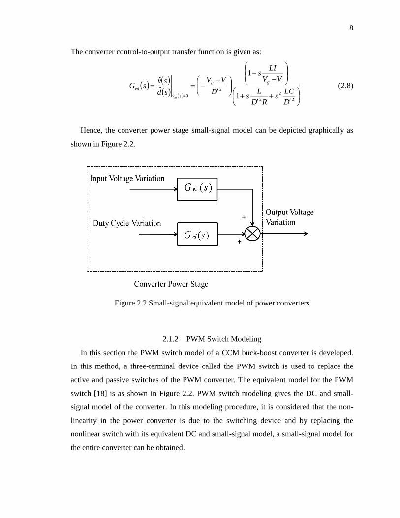
Hence, the converter power stage small-signal model can be depicted graphically as

shown in Figure 2.2.

Figure 2.2 Small-signal equivalent model of power converters

2.1.2 PWM Switch Modeling

In this section the PWM switch model of a CCM buck-boost converter is developed.

In this method, a three-terminal device called the PWM switch is used to replace the

active and passive switches of the PWM converter. The equivalent model for the PWM

switch [18] is as shown in Figure 2.2. PWM switch modeling gives the DC and small-

signal model of the converter. In this modeling procedure, it is considered that the non-

linearity in the power converter is due to the switching device and by replacing the

nonlinear switch with its equivalent DC and small-signal model, a small-signal model for

the entire converter can be obtained.

9

Figure 2.3 Equivalent DC and small signal model of PWM switch

By replacing this model in the buck-boost converter, the small signal transfer functions

[19] can be obtained.

The line to output transfer function of the buck-boost converter is given as:

( ) ( )( ) ( ) 12

1

ˆˆ

020

20ˆ ++

+==

= ss

s

svsvsG zn

sdinvin

ωξ

ω

ω (2.9)

Where,

( )( )[ ]( )( )

( )

==

+′+′+

=

′++

+′++′+=

RrrCr

rRLCRDrDDr

RDrrRLCLRrDrRrDDrC

CeC

zn

C

eL

LC

CCeL

,1

22

0

2

2

ω

ω

ξ

(2.10)

10

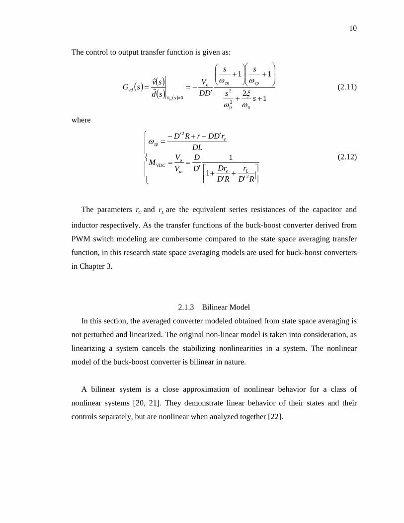
The control to output transfer function is given as:

( ) ( )( ) ( ) 12

11

ˆˆ

020

20ˆ ++

+

+

′−==

= ss

ss

DDV

sdsvsG zpzno

sv

vd

in

ωξ

ω

ωω (2.11)

where

′+

′+

′==

′++′−=

RDr

RDDrD

DVVM

DLrDDrRD

Lein

oVDC

ezp

2

2

1

1

ω

(2.12)

The parameters Cr and Lr are the equivalent series resistances of the capacitor and

inductor respectively. As the transfer functions of the buck-boost converter derived from

PWM switch modeling are cumbersome compared to the state space averaging transfer

function, in this research state space averaging models are used for buck-boost converters

in Chapter 3.

2.1.3 Bilinear Model

In this section, the averaged converter modeled obtained from state space averaging is

not perturbed and linearized. The original non-linear model is taken into consideration, as

linearizing a system cancels the stabilizing nonlinearities in a system. The nonlinear

model of the buck-boost converter is bilinear in nature.

A bilinear system is a close approximation of nonlinear behavior for a class of

nonlinear systems [20, 21]. They demonstrate linear behavior of their states and their

controls separately, but are nonlinear when analyzed together [22].

11

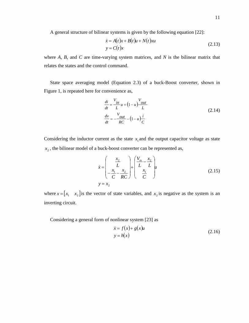
A general structure of bilinear systems is given by the following equation [22]:

( ) ( ) ( )( )xtCy

xutNutBxtAx=

++= (2.13)

where A, B, and C are time-varying system matrices, and N is the bilinear matrix that

relates the states and the control command.

State space averaging model (Equation 2.3) of a buck-Boost converter, shown in

Figure 1, is repeated here for convenience as,

( )

( )Ci

uRCoutV

dtdv

LoutV

uuLinV

dtdi

−−−=

−+=

1

1 (2.14)

Considering the inductor current as the state 1x and the output capacitor voltage as state

2x , the bilinear model of a buck-boost converter can be represented as,

2

1

2

21

2

xy

u

Cx

Lx

LV

RCx

Cx

Lx

xin

=

−+

−−=

(2.15)

where [ ]21 xxx = is the vector of state variables, and 2x is negative as the system is an

inverting circuit.

Considering a general form of nonlinear system [23] as

( ) ( )( )xhy

uxgxfx=

+= (2.16)

12

The functions ( )xf , ( )xg , and ( )xh of the bilinear buck-boost converter can be

represented as

( ) ( )

( ) 2

1

2

21

2

,

xxhCx

Lx

LV

xg

RCx

Cx

Lx

xfin

=

−=

−−=

(2.17)

2.2 Nonlinear System Structure

The bilinear model of the buck-boost converter can be converted into Isidori’s Normal

form if there exist a relative degree r for the system i.e. a non-singular co-ordinate

transformation.

A single-input single-output nonlinear system, of the form as given in Equation 2.16,

is said to have a relative degree r at a point x [23], where x is the state of the system at

time t such that ( ) 01 ≠− xhLL rfg .

i. ( ) 0=xhLL kfg for all x in a neighborhood of ox and all 1−< rk

ii. ( ) 01 ≠− orfg xhLL

where

( ) ( )∑= ∂∂

=n

ii

if xf

xxL

1

λλ (2.18)

The function (Equation 2.18) is the derivative of a vector λ along the direction of another

vector field f .

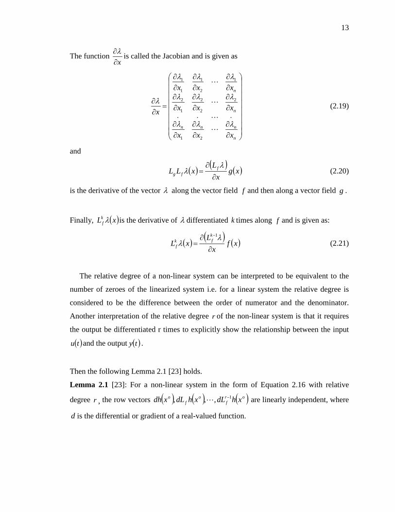
13

The function x∂

∂λ is called the Jacobian and is given as

∂∂

∂∂

∂∂

⋅⋅⋅∂∂

∂∂

∂∂

∂∂

∂∂

∂∂

=∂∂

n

nnn

n

n

xxx

xxx

xxx

xλλλ

λλλ

λλλ

λ

21

2

2

2

1

2

1

2

1

1

1

(2.19)

and

( ) ( ) ( )xgx

LxLL f

fg ∂

∂=

λλ (2.20)

is the derivative of the vector λ along the vector field f and then along a vector field g .

Finally, ( )xLkf λ is the derivative of λ differentiated k times along f and is given as:

( ) ( ) ( )xfx

LxL

kfk

f ∂

∂=

− λλ

1

(2.21)

The relative degree of a non-linear system can be interpreted to be equivalent to the

number of zeroes of the linearized system i.e. for a linear system the relative degree is

considered to be the difference between the order of numerator and the denominator.

Another interpretation of the relative degree r of the non-linear system is that it requires

the output be differentiated r times to explicitly show the relationship between the input

( )tu and the output ( )ty .

Then the following Lemma 2.1 [23] holds.

Lemma 2.1 [23]: For a non-linear system in the form of Equation 2.16 with relative

degree r , the row vectors ( ) ( ) ( )orf

of

o xhdLxhdLxdh 1,,, − are linearly independent, where

d is the differential or gradient of a real-valued function.

14

It can be concluded that a system of order n is of relative degree r if the following

proposition holds.

Proposition 2.1 [23]: Suppose the system has relative degree r at ox . Then nr ≤ and the

co-ordinate transformation is given as

( ) ( )( ) ( )

( ) ( )xhLx

xhLxxhx

rfr

f

1

2

1

−=

==

φ

φφ

(2.22)

If r is strictly less than n , it is always possible to find rn − functions ( ) ( )xx nr φφ ,1+ such

that the mapping

( )( )

( )

=

x

xx

nφ

φφ

1

(2.23)

has a jacobian matrix nonsingular at ox and qualifies as a local coordinate transformation

in a neighborhood of ox . The value at ox of these additional functions can be fixed

arbitrarily. Moreover, it is always possible to choose ( ) ( )xx nr φφ ,1+ such that ( ) 0=xL igφ

for all nir ≤≤+1 and all x around ox .

Hence, the state-space description of the system (Equation 2.16) in the normal form

[23] is given as follows:

( ) ( )( )

( )zqz

zqzuzazbz

zz

zzzz

nn

rr

r

rr

=

=+=

=

==

++

−

11

1

32

21

(2.24)

15

For a buck-boost converter system (Equation 2.17), the relative degree is 1=r as

( ) ( ) ( ) 0]10[ 1

1

2

≠=

−=

∂∂

=Cx

Cx

Lx

LV

xgxxhxhL

in

g (2.25)

As the relative degree is one for a second order system, there exist a non-singular co-

ordinate transformation and therefore the normal form is

( ) ( )

( )

( )

==

−+==

===

2

22

22

122

211

22xxhy

VLx

Lx

Cxxz

xxhxz

inφ

φ

(2.26)

The output voltage of an inverting buck-boost converter is 02 <x and as the buck-

boost converter is considered to be operating in CCM 01 >x . Therefore, 02 >z for all

values and the inverse transformation exists and can be obtained as

=

−+=

12

21

121 22

zx

Lz

LVzzCx in

(2.27)

The buck-boost converter system in the new coordinates ( )21 , zz , i.e. the normal form,

is represented by

( )

1

21

12

211

2

21

1211

22

2211

zy

Lzz

LVzC

LCV

RLCzzVz

Lzz

LVzC

Cuz

RCz

ininin

in

=

−++

−=

−+

−−−=

(2.28)

The advantage of the normal form of the system is the structure, which is taken

advantage of in different controls like exact linearization, due to which many important

16

properties of the system can be obtained just by inspection. From Equation 2.28, it can be

said that the relative degree of the buck-boost converter system is one, as the first

equation explicitly contains the input term ( )tu . The zero dynamics of a non-linear system

can also be easily obtained from the normal form.

2.3 Zero Dynamics

The zero dynamics of a non-linear system are analogous to the zeros of the transfer

function in a linear system. A system with relative degree r that is strictly less than the

order of the system n is said to have zero dynamics of the order rn − . If nr = the system

does not have any unseen internal dynamics and it also implies that the transfer function

of the linear system has no zeros. Zero dynamics of a system are the hidden internal

dynamics when the initial conditions of the system and the input are constrained to make

the output of the system zero [23].

The zero dynamics of a nonlinear system can be easily obtained from the Isidori’s

Normal form, by zeroing the output. If a nonlinear system (Equation 2.16) has a relative

degree r then the state vector z can be grouped into the following two vectors as given

below:

=

=

+

n

r

r z

z

z

z

11

, ηξ (2.29)

Then the normal form can be written as:

( ) ( )( )ηξη

ηξηξ,

,,1

32

21

quabz

zz

zzzz

r

rr

=+=

=

==

−

(2.30)

17

When the output of the system is identical to zero its state is constrained to evolve such

that ( )tξ is identically zero [23]. Then the zero dynamics are given by the following

equation as:

( ) ( )( )tqt ηη ,0= (2.31)

then the unique input to the system is given as:

( ) ( )( )( )( )tatbtu

ηη,0,0

−= (2.32)

For the buck-boost converter system the zero dynamics are obtained by zeroing the

output in Equation 2.26, then the following equation is obtained,

22 2CzLCVz in= (2.33)

Phase plane [25] is a tool used to analyze the stability of zero dynamics. This method

is used to graphically analyze how the system trajectories change with the state variable

from which the stability of the system can be commented. The phase plane plot of the

zero dynamics is shown in Figure 2.4.

As the phase plane trajectories diverge in Figure 2.4, the zero dynamics of the

capacitor voltage in a buck-boost converter are not stable; this behavior is due to the non-

minimum phase nature of these converters with respect to capacitor voltage. Hence, the

zero dynamics of the non-minimum phase voltage of the buck-boost converter are

unstable.

18

Figure 2.4 Phase plane plot of zero dynamics of capacitor voltage

2.4 Passivity

A system is said to be passive if its rate of energy storage is less than the rate of

supply energy i.e. the system dissipates more energy than it stores. As a result, the energy

storage function of the system is less than the supply rate energy function. Passivity can

be formalized by the following definitions. Consider a nonlinear system, H, defined as

( )( )

==

=uxhyuxfx

H,,

(2.34)

Definition 2.1 Supply Rate [25]: The supply rate ( ) ( ) ( )( )tytuwtw ,= is a real valued

function defined on YU × , such that for any ( ) Utu ∈ and Xxo ∈ and

( ) ( )( )uxtthty ,,, 00φ= , ( )tw satisfies

( ) ∞<∫ dttwt

t

1

0

(2.35)

for all 001 ≥≥ tt .

0 2 4 6 8 10 120

2

4

6

8

10

12

14Phase Plane Plot of Zero Dynamics of Output Voltage

z2

z2do

t

19

Definition 2.2 Dissipative Systems [25]: System H with supply rate ( )tw is said to be

dissipative if there exists a nonnegative real function ( )xS : +ℜ→X , called the storage

function, such that, for all 01 ≥≥ tt , Xx ∈0 and Uu∈ ,

( ) ( ) ( )∫≤−1

0

01

t

t

dttwxSxS (2.36)

or

( )( ) ( )twdt

txdS≤ (2.37)

Where ( )uxttx ,,, 0011 φ= and +ℜ , is a set of nonnegative real numbers. A Lyapunov

candidate of the system can be used as Storage Function ( )xS .

Definition 2.3 Passive Systems [25]: A system is said to be passive if it is dissipative

with respect to the following supply rate

( ) ( )( ) ( ) ( )tytutytuw T=, (2.38)

and the storage function ( )xS satisfies ( ) 00 =S .

Passivity is an input-output property, and it depends on how the output of the system

is defined. Consider the buck-boost converter system in its original representation

(Equation 2.16) with a positive definite storage function ( ) 22

21 2

121 CxLxxS += . In order to

investigate this input-output property, consider, for now, the output as the current and

define a bilinear supply rate ( ) 1xVuyutw inT ⋅⋅== , where inVu ⋅ is the input to the circuit

with current 1x as output. Then the following can be shown:

( ) ( )twRxxuVxS in ≤−=

22

1 (2.39)

Hence, the buck-boost converter is passive when the output defined is the inductor

current.

20

The following theorem encapsulates the passivity properties for nonlinear systems as

Theorem 2.1 [25]: A system H with a constant rank ( ) xhLg in a neighborhood of 0=x ,

with a 2C storage function ( )xS which is positive definite, is passive, then:

1. ( )0hLg is nonsingular and H has relative degree 1,,1 .

2. The zero dynamics of H exists locally at ,0=x and H is weakly minimum phase.

As the phase plane plot (Fig. 2.4) reveals, the output voltage zero dynamics are

unstable, i.e. non minimum phase. Therefore from theorem 2.1 it can be inferred that the

buck-boost converter is not passive respect to the output voltage.

Passivity is an input-output property, and does not provide information about the state

of the system. But, the Kalman-Yacubovich-Popov property relates passivity of the

system with the state of the system. It relates the storage function of the system with the

Lyapunov candidate of the system and is given as follows:

Definition 2.4 Kalman-Yacubovich-Popov Property [25]: Consider a control affine

system without throughput (2.16) where nXx ℜ∈∈ , mUu ℜ⊂∈ and mYy ℜ⊂∈ . It is

said to have the Kalman-Yacubovich-Popov (KYP) property if there exists a 1C

nonnegative function ( ) +ℜ→XxS : , with ( ) 00 =S such that

( ) ( ) ( ) 0≤∂

∂= xf

xxSxSLf (2.40)

( ) ( ) ( ) ( )xhxgxxSxSL T

g =∂

∂= (2.41)

for each Xx∈ .

A system H of the form (Equation 2.16) which has the KYP property is passive, with a

storage function ( )xS and conversely, a passive system having a 1C storage function has

the KYP property [25]. This proposition is used in Chapter 4 to derive the gain

constraints for a parallel interconnection in a feed-forward passivation procedure. .

21

PARALLEL COMPENSATION APPROACH 3.

3.1 Motivation

In this chapter, the parallel compensation approach is introduced to overcome the

drawbacks of the existing linear control methods [6, 7] discussed in Chapter 1. It will be

shown at the end of this chapter that this method accelerates the transient response of the

converter, considerably removes undershoot in the response, reduces the oscillations in

the transient response, and directly regulates the voltage instead of using multi-loop

current mode control [7]. The effectiveness of this method can be verified from the

simulation results carried out on the buck-boost converter.

State space averaging method is used to represent the buck-boost converter

mathematically. The small-signal control-to-output transfer function and the line-to-

output transfer function of the buck-boost converter (Equations 2.6-2.8), derived in

Chapter 2, are used in the process of designing a compensator. The non-minimum phase

control-to-output transfer function is decoupled from the minimum phase line-to-output

transfer function and a parallel compensator is connected in parallel to the non-minimum

phase transfer function. The new replacement plant is compensated in such a way that the

system exhibits minimum phase characteristics.

An effective way to design a compensator for the non-minimum phase systems is to

use strictly positive real form of the system [27, 28]. Parallel feed-forward compensators

can be used to convert any plant to an almost strictly positive real system [29]. Then the

control can be achieved by using output feedback techniques.

22

Parallel compensation techniques have been successfully implemented [30, 31] and

have proven to be efficient and stable control approaches for non-minimum phase

systems than pole-zero cancellation technique [32]. Pole-zero cancellation generates

hidden modes that may cause instabilities, thus, cannot be universally used in non-

minimum phase systems.

There are different methods in deriving the transfer function of an augmented plant

and the parallel compensator. The principle of transforming the configuration of a non-

minimum phase plant to minimum phase is introduced in [33]. This technique uses a feed

through compensation to obtain a minimum-phase augmented plant and uses a high gain

feedback control to stabilize the system [33]. The transfer function of the compensator in

[33] is derived by using the transmission-zero-assignment technique [34]. Gessing [35,

36] have also proposed ways of changing non-minimum phase plants into minimum

phase. They have classified the control problems of regulation, tracking or disturbance

rejection and specially designed replacement plants for each problem at hand. General

approach to compensator design depends on the application purposes [34-36]. The

control problem of the converter, considered in this thesis, falls under the category of

voltage regulation [35] and the method outlined in [35] is adopted here.

3.2 Undershoot and Non-minimum Phase Zeros

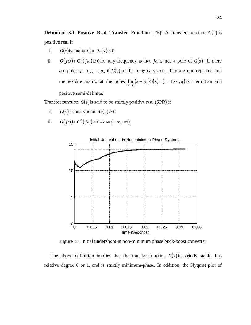
It has been studied and observed [9, 38] that in a non-minimum phase system with odd

number of positive zeros, the system response gives rise to an initial undershoot. In such

a case, the coefficients of the numerator polynomial of a system are not all positive [38],

thus non-Hurwitz. This can be verified in the case of buck-boost converter system from

its control-to-output transfer function (Equation 2.8) given by:

( ) ( )( ) ( )

′+

′+

−−

′−

−===

22

2

20ˆ 1

1

ˆˆ

DLCs

RDLs

VVLIs

DVV

sdsvsG gg

svvd

in

(3.1)

23

It can be observed that all of the coefficients of the numerator polynomial in Equation

3.1 are not positive. The undershoot in a system is undesirable as the output initially

tends in the opposite direction of the final value, as a result delay is introduced into the

system.

The physical significance behind the undershoot due to the right half-plane zeroes in

converters can be explained as follows. The average diode current of the converter in

Figure 2.1 is related to the average inductor current [17] as follows:

ss TLTD idi ′= (3.2)

where sT is the switching interval.

The average diode current Di is equal to the load current. When a step increase in duty

cycle is applied, Di decreases and the capacitor begin to discharge and the voltage

across the capacitor drops. However, the increased duty cycle causes a slow increase in

the inductor current as a result Di increases again and the voltage across the capacitor

starts increasing. This delay in the rise of the inductor current is not a desirable

phenomenon as it causes undershoot in the system and is a destabilizing effect. In this

research, this problem is addressed and the parallel compensation approach is provided as

a solution to the problem. The following behavior is observed in the simulations of the

buck-boost converter without any compensation as shown in Figure 3.1.

3.3 Positive Real Transfer Function

Positive real systems have many important properties with regard to stability analysis

and in the generation of Lyapunov functions. A passive linear system (Equation 2.38) is

strictly positive real, and vice versa. The following definition can be given with regard to

a positive real transfer function.

24

Definition 3.1 Positive Real Transfer Function [26]: A transfer function ( )sG is

positive real if

i. ( )sG is analytic in ( ) 0Re >s

ii. ( ) ( ) 0* ≥+ ωω jGjG for any frequency ω that ωj is not a pole of ( )sG . If there

are poles qppp ,,, 21 of ( )sG on the imaginary axis, they are non-repeated and

the residue matrix at the poles ( ) ( ) ( )qisGps ips i

,,1lim =−→

is Hermitian and

positive semi-definite.

Transfer function ( )sG is said to be strictly positive real (SPR) if

i. ( )sG is analytic in ( ) 0Re ≥s

ii. ( ) ( ) ( )+∞∞−∈∀>+ ,0* ωωω jGjG

Figure 3.1 Initial undershoot in non-minimum phase buck-boost converter

The above definition implies that the transfer function ( )sG is strictly stable, has

relative degree 0 or 1, and is strictly minimum-phase. In addition, the Nyquist plot of

0 0.005 0.01 0.015 0.02 0.025 0.03 0.0350

5

10

15

Time (Seconds)

Initial Undershoot in Non-minimum Phase Systems

25

( )ωjG lies entirely in the right half complex plane or the phase shift of the system is

always within the range of ( ) 90,90− .

In order to achieve the objectives as specified in Chapter 1, it is desired that the non-

minimum phase control-to-output transfer function of buck-boost converter be converted

to SPR/PR, such that the system be converted to a minimum phase system. The transfer

function approach is considered here, as a linear small-signal model of buck-boost

converter is adopted in parallel compensation approach. The process of designing a

compensator is detailed in the following sections.

3.4 Control Structure

The control scheme given to achieve the stated objectives is shown in Figure 3.2. As

can be observed in Figure 3.2, the compensation is applied only to the decoupled non-

minimum phase control-to-output transfer function. Then voltage regulation can be

achieved by the use of a simple proportional controller. The control structure for the

buck-boost converter plant is as shown in Figure 3.3. The next section gives the design

procedure for the parallel compensator.

3.5 Design of Parallel Compensator for Voltage Regulation Application

In this section the parallel compensator for the control-to-output transfer function is

derived. The technique outlined in [35] is adopted for deriving the replacement plant for a

buck-boost converter. There are other techniques to accomplish this task such as the

transmission zero assignment technique [34]. This technique uses Eigen value assignment

technique to place the transmission zeros in the desired positions. Moreover, the

complexity of the procedure increases as buck-boost converter is also non-linear in nature.

So the following method [35] of deriving the replacement plant for the buck-boost

converter control-to-output transfer function has been adopted.

26

A first order shunt system is taken as the transfer function for the replacement plant.

Therefore, the replacement plant is selected in such a way that it is SPR, then the non-

minimum phase control-to-output transfer function is compensated to become a minimum

phase system. The only criterion to be satisfied for the application of using this kind of

replacement plant is that the original open-loop converter control-to-output transfer

function should be stable.

The control-to-output transfer function of buck-boost converter (Equation 2.8) is

stable as the denominator polynomial is Hurwitz. Hence, all the poles of the buck-boost

converter are in the left-half plane and the open-loop transfer function is stable.

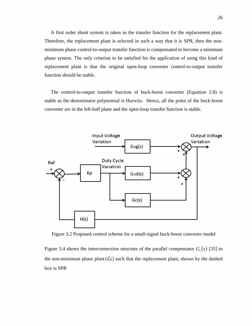
Figure 3.2 Proposed control scheme for a small-signal buck-boost converter model

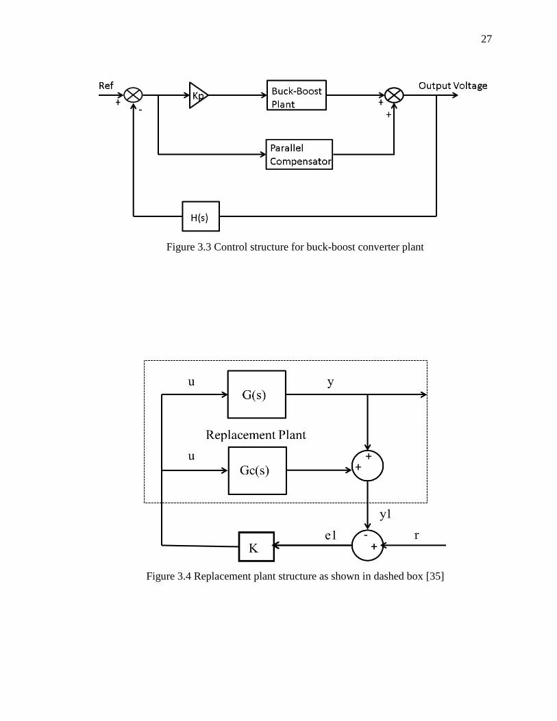
Figure 3.4 shows the interconnection structure of the parallel compensator ( )sGc [35] to

the non-minimum phase plant ( )sG such that the replacement plant, shown by the dashed

box is SPR

27

Figure 3.3 Control structure for buck-boost converter plant

Figure 3.4 Replacement plant structure as shown in dashed box [35]

28

The non-minimum phase transfer function for which a replacement transfer function is

to be derived is given as below:

)()(

)()()(

sMsL

sUsYsG == (3.3)

Then the transfer function of the parallel compensator which is to be connected in parallel

to the above non-minimum phase plant is given as:

( ) ( )( ) ( ) ( )sGsGsUsYsG c

c −== 1 (3.4)

The transfer function of the replacement plant, which is minimum phase, is given by

)()()()(

)()()()()(

11

1

sGsGsGsG

sGsGsUsYsG cr

=−+=

+== (3.5)

The transfer function of the stable replacement plant )(1 sG is chosen as,

( )11 +

=Ts

ksG o (3.6)

where the constant ok is given [35] as:

( )0Gko = (3.7)

From Equation 3.6 it can be said that ( )sG1 is SPR as the relative degree is one,

minimum-phase and stable. The condition to be satisfied by the original plant and the

replacement plant is that steady state value of the original plant should be equal to the

steady state value of the replacement plant as:

( ) ( )001 GG = (3.8)

Now for the buck-boost control-to-output non-minimum phase transfer function given as

29

( )

′+

′+

−−

′−

−=

22

2

2

1

1

DLCs

RDLs

VVLIs

DVV

ksG ggvd (3.9)

The replacement plant transfer function is as given below and is derived based on the

procedure outlined above:

( ) ( ) kD

VVglsT

lsGvd 21 ',

1−

−=+

= (3.10)

Thus, the parallel compensator using Equation 3.4 for the buck-boost converter

control-to-output transfer function is given as:

( )2

22

2

''1

1

1DLCs

RDsL

VVLIs

DVV

sTlsG gg

c

++

−−

′−

−−+

= (3.11)

where the gain k is a proportional constant which is known and the time constant T is a

positive number. It has been observed in simulations that the smaller the time constant T,

the faster the response of the system.

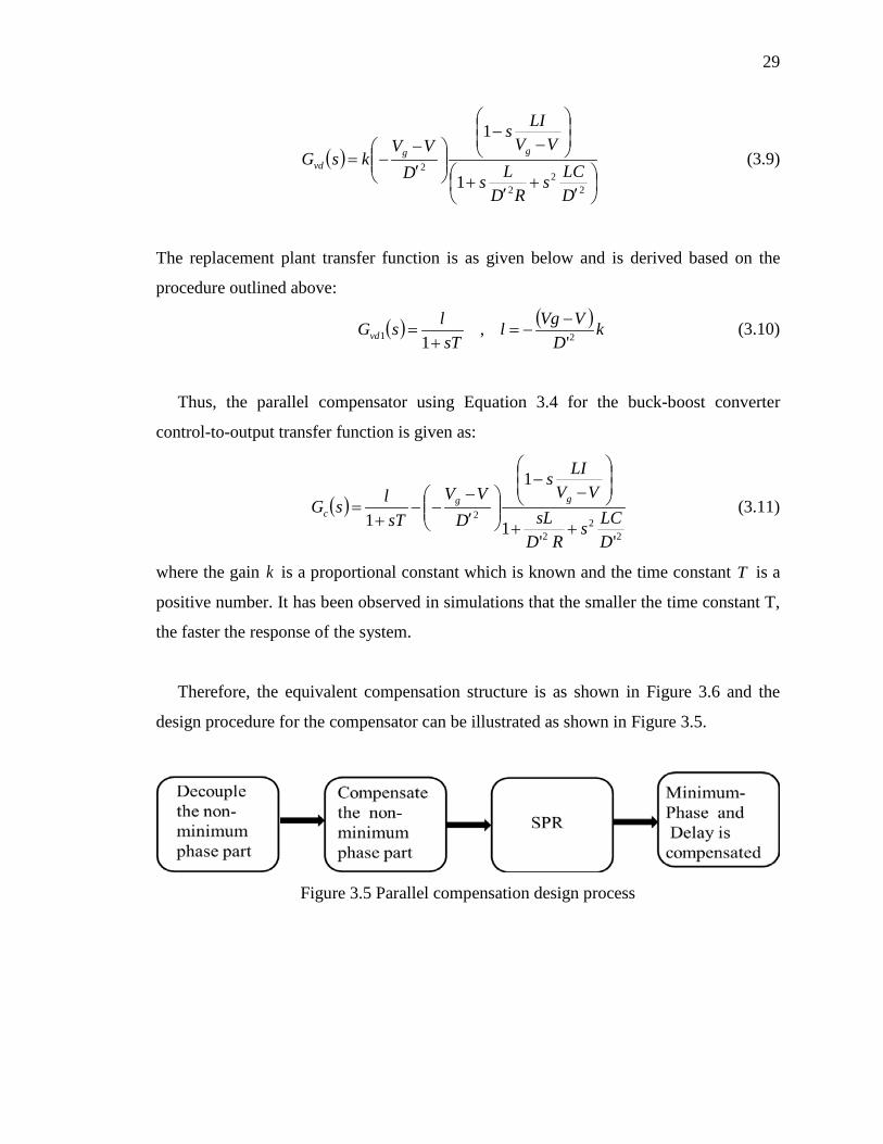
Therefore, the equivalent compensation structure is as shown in Figure 3.6 and the

design procedure for the compensator can be illustrated as shown in Figure 3.5.

Figure 3.5 Parallel compensation design process

30

Figure 3.6 Equivalent compensation structure [35]

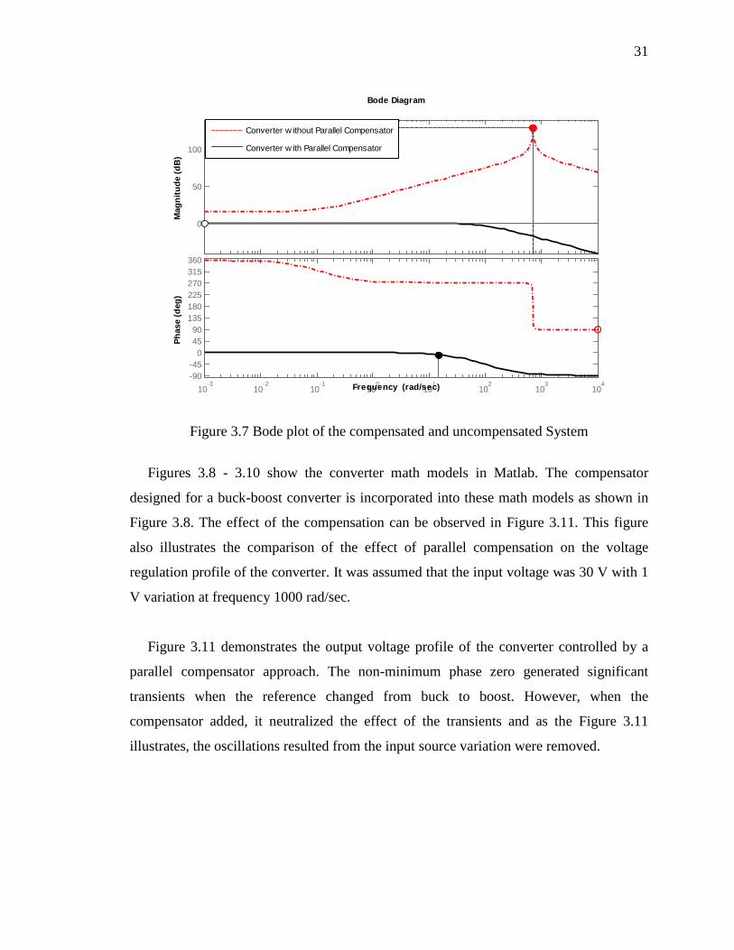
3.6 Stability

To understand the effect of the parallel compensator on the closed loop stability of a

buck-boost converter, the bode diagram of the converter control-to-output transfer

functions with and without compensation is provided in Figure 3.7. It can be observed

that the phase of the compensated system is in the range of ( ) 90,90− satisfying the

requirement of SPR system.

3.7 Simulation Results

The simulations are carried out on the buck-boost converter with the following

parameters: VVmFCHLR g 30,1,100,10 ===Ω= µ . The derived math model of

the buck-boost converter using state-space averaging (Equations 2.7-2.8) is represented

mathematically in Matlab.

31

Figure 3.7 Bode plot of the compensated and uncompensated System

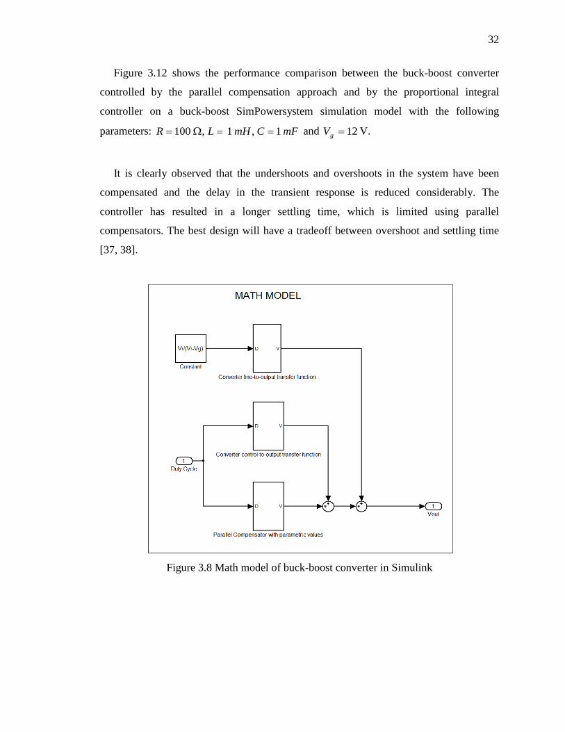
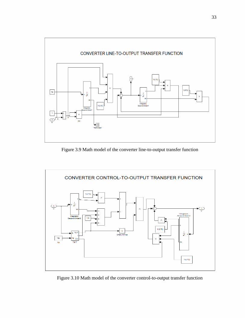
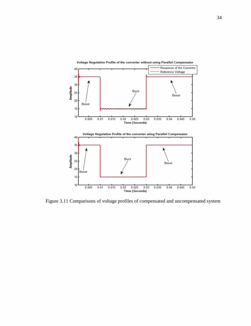
Figures 3.8 - 3.10 show the converter math models in Matlab. The compensator

designed for a buck-boost converter is incorporated into these math models as shown in

Figure 3.8. The effect of the compensation can be observed in Figure 3.11. This figure

also illustrates the comparison of the effect of parallel compensation on the voltage

regulation profile of the converter. It was assumed that the input voltage was 30 V with 1

V variation at frequency 1000 rad/sec.

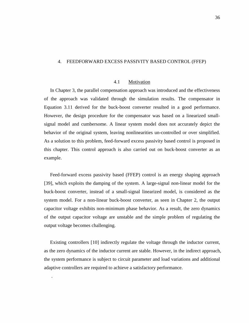
Figure 3.11 demonstrates the output voltage profile of the converter controlled by a

parallel compensator approach. The non-minimum phase zero generated significant

transients when the reference changed from buck to boost. However, when the

compensator added, it neutralized the effect of the transients and as the Figure 3.11

illustrates, the oscillations resulted from the input source variation were removed.

0

50

100

Mag

nitu

de (d

B)

10-3

10-2

10-1

100

101

102

103

104

-90-45

04590

135180225270315360

Phas

e (d

eg)

Bode Diagram

Frequency (rad/sec)

Converter w ithout Parallel Compensator

Converter w ith Parallel Compensator

32

Figure 3.12 shows the performance comparison between the buck-boost converter

controlled by the parallel compensation approach and by the proportional integral

controller on a buck-boost SimPowersystem simulation model with the following

parameters: mFCmHLR 1,1,100 ==Ω= and 12=gV V.

It is clearly observed that the undershoots and overshoots in the system have been

compensated and the delay in the transient response is reduced considerably. The

controller has resulted in a longer settling time, which is limited using parallel

compensators. The best design will have a tradeoff between overshoot and settling time

[37, 38].

Figure 3.8 Math model of buck-boost converter in Simulink

33

Figure 3.9 Math model of the converter line-to-output transfer function

Figure 3.10 Math model of the converter control-to-output transfer function

34

Figure 3.11 Comparisons of voltage profiles of compensated and uncompensated system

35

Figure 3.12 Comparison of voltage profile with a compensator and a PI controller

0 0.5 1 1.5 2 2.5 30

20

40

60

80

Time (Seconds)

Ampl

itude

Voltage Regulation Profile of the Converter using Proportional Integral Controller

0 0.5 1 1.5 2 2.5 30

5

10

15

20

25

Time (Seconds)

Ampl

itude

Voltage Regulation Profile of the Converter using Parallel Compensator

Reference voltageResponse of the Converter

Boost

Buck

Boost

Boost

Buck

Boost

36

FEEDFORWARD EXCESS PASSIVITY BASED CONTROL (FFEP) 4.

4.1 Motivation

In Chapter 3, the parallel compensation approach was introduced and the effectiveness

of the approach was validated through the simulation results. The compensator in

Equation 3.11 derived for the buck-boost converter resulted in a good performance.

However, the design procedure for the compensator was based on a linearized small-

signal model and cumbersome. A linear system model does not accurately depict the

behavior of the original system, leaving nonlinearities un-controlled or over simplified.

As a solution to this problem, feed-forward excess passivity based control is proposed in

this chapter. This control approach is also carried out on buck-boost converter as an

example.

Feed-forward excess passivity based (FFEP) control is an energy shaping approach

[39], which exploits the damping of the system. A large-signal non-linear model for the

buck-boost converter, instead of a small-signal linearized model, is considered as the

system model. For a non-linear buck-boost converter, as seen in Chapter 2, the output

capacitor voltage exhibits non-minimum phase behavior. As a result, the zero dynamics

of the output capacitor voltage are unstable and the simple problem of regulating the

output voltage becomes challenging.

Existing controllers [10] indirectly regulate the voltage through the inductor current,

as the zero dynamics of the inductor current are stable. However, in the indirect approach,

the system performance is subject to circuit parameter and load variations and additional

adaptive controllers are required to achieve a satisfactory performance.

.

37

This, in turn, tends to increase the complexity of the system. In this research, FFEP

control is proposed as a solution and aims to achieve direct regulation of non-minimum

output voltage. It has also been verified through simulation and experimental results that

the system performance is not significantly affected by the load variations and does not

call for additional advanced controllers.

FFEP control uses the principle of passivity as a design tool. It has been investigated

in Chapter 2 that the buck-boost converter system is not passive when the output is the

capacitor voltage. It is due to the non-minimum phase behavior of the capacitor voltage.

In FFEP control, direct regulation of voltage is achieved by making the open-loop buck-

boost converter passive when the output is the capacitor voltage. In order to attain

passivity in the converters, the damping of the converter system i.e. the degree of

passivity need to be modified.

In FFEP control, it is shown that a parallel interconnection to the open-loop system

can achieve exponential stability of the zero dynamics of the output voltage. An excess

passive system is used to compensate for the shortage of passivity in the buck-boost

converter to reduce the non-minimum phase behavior. To achieve passive system, the

degree of passivity in the system is characterized from passivity indices rather than from

the system’s energy function.

The noteworthy feature of FFEP control lies in its simplicity and its effectiveness.

Though, different solutions [40, 41] to the problem of direct regulation of non-minimum

phase voltage have been previously proposed, they rely on circuit level energy

descriptions whereas FFEP control which is based on a system level description. Chapter

5 compares the two methods of approach and shows the merit of FFEP over [40, 41]. The

following sections of Chapter 4 provide detailed information regarding the FFEP control

It has to be pointed out that the motivation for FFEP control for non-minimum phase

power converters is inspired from process control [44] and networked control systems

38

[43]. The concept of compensating for the shortage of passivity through system

interconnection has been thoroughly explored in applications relating to pH process

control, heat distillation columns, robotic manipulators [42], and in large interconnected

systems. The novelty of this research lies in the identification and application of this

concept to non-minimum phase power converters, in order to achieve simple effective

solution for the problem of direct regulation of non-minimum phase voltage.

4.2 Passivity Indices

In FFEP control, the degree of passivity in a system [24, 26, 45], as an index to

measure the passivity, is quantified by passivity indices. The passivity indices indicate

either excess or shortage of passivity. The following two definitions [26] can be given

with regard to excess and shortage of passivity.

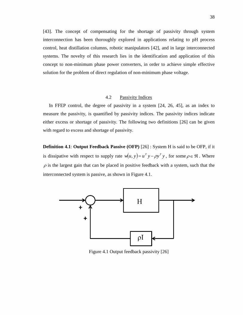
Definition 4.1: Output Feedback Passive (OFP) [26] : System H is said to be OFP, if it

is dissipative with respect to supply rate ( ) yyyuyuw TT ρ−=, , for some ℜ∈ρ . Where

ρ is the largest gain that can be placed in positive feedback with a system, such that the

interconnected system is passive, as shown in Figure 4.1.

Figure 4.1 Output feedback passivity [26]

39

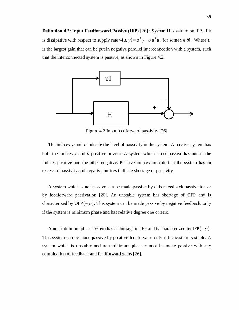
Definition 4.2: Input Feedforward Passive (IFP) [26] : System H is said to be IFP, if it

is dissipative with respect to supply rate ( ) uuyuyuw TT υ−=, , for some ℜ∈υ . Where υ

is the largest gain that can be put in negative parallel interconnection with a system, such

that the interconnected system is passive, as shown in Figure 4.2.

Figure 4.2 Input feedforward passivity [26]

The indices ρ and υ indicate the level of passivity in the system. A passive system has

both the indices ρ and υ positive or zero. A system which is not passive has one of the

indices positive and the other negative. Positive indices indicate that the system has an

excess of passivity and negative indices indicate shortage of passivity.

A system which is not passive can be made passive by either feedback passivation or

by feedforward passivation [26]. An unstable system has shortage of OFP and is

characterized by OFP ( )ρ− . This system can be made passive by negative feedback, only

if the system is minimum phase and has relative degree one or zero.

A non-minimum phase system has a shortage of IFP and is characterized by IFP ( )υ− .

This system can be made passive by positive feedforward only if the system is stable. A

system which is unstable and non-minimum phase cannot be made passive with any

combination of feedback and feedforward gains [26].

40

The technique of feedback passivation [46] is quite popular and makes use of

feedback to render a system passive. However, the relative degree and zero-dynamics of

a system are invariant under feedback, and any system irrespective of its relative degree

whose zero dynamics with respect to the output are not minimum phase, cannot be made

passive via feedback. Buck-boost converters fall under the category of a system whose

relative degrees is one and has unstable output voltage zero dynamics. Therefore, direct

voltage regulation of non-minimum buck-boost converter can be made possible only by

feedforward passivation [26].

It should be noted that more general definitions for the supply rate functions can be

used other than given in Definition 1 and Definition 2, to simultaneously obtain the IFP

and OFP indices. Some such supply rates [26] can be given as:

( ) ( ) ( )yuuuyyuw TTT ρυ −−=, (4.1)

or

( ) ( )( ) ( ) ( ) ( ) ( ) ( ) ( )tRututSytutQytytytuw TTT ++= 2, (4.2)

where mmSRQ ×ℜ∈,, are constant weighting matrices, with matrices Q and R being

symmetrical.

Note 4.1: The following general statement should be recalled with regard to classical

control. Feedback structure in a system affects the poles of the system i.e. the system

stability, and Feedforward structure in a system effects the zeros of the system i.e. zero

dynamics.. Therefore, feedback passivation applied on a system does not influence the

zero dynamics and relative degree of the system. Similarly feedforward passivation

cannot influence the free dynamics of the system i.e. the stability of the system.

4.3 Passivity in Relation to Stability and Positive Realness

The concept of stability, passivity and positive realness are interrelated and this

section explores their relationship. A passive system is stable when it is unforced i.e.

when the input 0=u . This relation between passivity and stability can be formally given

41

prior to which certain definitions like zero-state observability (ZSO) and zero-state

detectability (ZSD) are to be stated.

Definition 4.3 ZSO and ZSD [26]: A system ( )( )

==

uxhyuxfx

H,,

:

is ZSO if for any Xx∈ ,

( ) ( )( ) 0,00,,, 00 ≥≥∀== ttxtthty φ 0=ximplies (4.3)

and the system is locally ZSO if there exists a neighborhood nX of 0, such that for all

nXx∈ , Equation 4.3 holds. The system is ZSD if for any Xx∈ ,

( ) ( )( ) ( ) 00,,,lim0,00,,, 000 =≥≥∀==∞→

xttimpliesttxtthtyt

φφ (4.4)

and the system is locally ZSD if there exists a neighborhood nX of 0, such that for all

nXx∈ Equation 4.4 holds.

The following theorem relates passivity and stability.

Theorem 4.1 Passivity and Stability [24]: The passive system H with a 1C storage

function S and ( )uxh , be 1C in u for all x . Then the following properties hold:

i. If S is positive definite, then the equilibrium 0=x of H with 0=u is stable

ii. If H is ZDS, then the equilibrium 0=x of H with 0=u is stable

iii. When there is no throughput, ( )xhy = , then the feedback yu −= achieves

asymptotic stability of 0=x if and only if H is ZSD.

where 1C of a function indicates that the derivate of the function exists and is continuous.

A system is said to be positive real if the following relation holds [26]:

( ) ( ) 0,0 01

1

0

≥≥∀≥∫ ttdttutyt

t

T (4.5)

From Equation 2.36 it can be inferred that a positive real system is passive and vice versa.

42

4.4 Exponential Stability and Passivity Indices of Buck-Boost Converter

The stability of a nonlinear system can be given by various definitions, depending on

the degree of stability in the system. A nonlinear system can have different equilibriums

unlike a linear system [26]. So the stability in a non-linear system is with respect to the

individual equilibrium point. It is very likely that some equilibrium points in a non-linear

system are stable and some of them from the same system are unstable. The following

definition is the stability of the system in the sense of Lyapunov.

Definition 4.4 Stability in the sense of Lyapunov [25]: The equilibrium state 0=X is

said to be stable if for any 0>R , there exists 0>r , such that if ( ) rx <0 , then

( ) Rtx < for all 0≥t . Otherwise, the equilibrium point is unstable.

Definition 4.4 implies that for a stable system the state trajectories, originating from a set

of initial states, are confined to a bounded region of a certain radius. Definition 4.4 can be

said to be an unconstrained definition of stability and does not give indicate how fast the

system trajectories converge to the bounded region.

The following definition can be given with regard to asymptotic stability.

Definition 4.5 Asymptotic Stability [25]: An equilibrium point 0 is asymptotically

stable if it is stable, and if in addition there exists some 0>r such that ( ) rX <0 implies

that ( ) 0→tX as .∞→t

Asymptotic stability gives an estimate about the convergence of the system state

trajectories, and is a strong definition of stability than the definition of stability in the

sense of Lyapunov. Exponential stability of the system has faster rate of convergence of

system states than asymptotic stability and is given by Definition 4.6.

43

Definition 4.6 Exponential Stability [25]: A system is exponentially stable [25] if there

exist two strictly positive numbers α and λ such that,

( ) ( ) textxt λα −≤>∀ 0,0 (4.6)

In some ball rB around the origin.

Hence the following order of precedence can be given with regard to how fast the system

trajectories converge.

StabilitylExponentiaStabilityAymptoticLyapunovofsensetheinStability ⇒⇒

The above distinction between the degrees of stability in a system is vital, especially

when the system comprises of several interconnections between different sub-systems.

The interactions between the sub-systems influence the stability of the overall system, so

it is critical to mark the degree of stability of each sub-system.

In this research on FFEP control, a more constrained definition of stability is imposed

on buck-boost converter, which is justified in Section 4.10. The following arguments can

be given with regard to exponential stability of the buck-boost converter.

To demonstrate the exponential stability of the output voltage of the buck-boost

converter, characteristic equation of the buck-boost converter is used. When the switch Q

in Figure 2.1 is on or off mode, the output voltage x2 is in charging or discharging mode

of operation respectively. In either case, a general form of this state variable can be

expressed as tAex λ−=2 (4.7)

where A is a negative coefficient, as the buck-boost converter is an inverting circuit, and

λ is the time constant of the circuit defined as:

RC1

=λ (4.8)

44

In an RLC circuit, analyzed separately in two modes of buck-boost operation, x2 can be

expressed as tt eAeAx 21

212λλ −− += (4.9)

where 1λ and 2λ are the circuit time constants and

LCRCRC

LCRCRC

12

12

1

12

12

1

2

2

2

1

−

+=

−

−=

λ

λ (4.10)

In a physically realizable circuit, the time constants 1λ , 2λ are strictly positive values.

Hence, the state 2x of the buck-boost system, which is the output voltage, converges to

the origin exponentially. Thus, buck-boost converter is exponentially stable.

Note 4.2: The argument (Equations 4.7-4.10) with regard to exponential stability of the

buck-boost converter when the output is the capacitor voltage may be misleading, with

the statement that the zero dynamics of the output capacitor voltage (Equation 2.33) are

unstable. In order to clarify, another definition of zero dynamics need to be highlighted

from Brynes and Isidori’s pioneering work [49] on zero dynamics of a nonlinear system.

For a nonlinear system of the form (Equation 2.16), which is decomposed into observable

and unobservable components, the zero dynamics of a system can be considered as the

internal dynamics of the unobservable component. Hence, stability of the system i.e.

observable part of the system does not imply stability of the unobservable component i.e.

the zero dynamics, which is the cause of all complications.

IFP and OFP passivity indices of the buck-boost converter system can be obtained by

considering the buck-boost converter system in its original bilinear representation

(Equation 2.15) with a positive definite storage function,

( ) 22

21 2

121 CxLxxS += (4.11)

and by considering a more general definition for the supply rate (Equation 4.1)

45

( ) ( )2222 inin

TTT uVxxuVuuyyyutw υρυρ −−=−−= (4.12)

and the following relation is given

( ) ( ) ( )222

222

1 xuVxuVRxxuVxS ininin −−≤−= ρυ (4.13)

It can be observed that R1

=ρ is positive and 1x>υ is negative, depicting a shortage of

IFP ( )υ− and an excess of OFP ( )ρ in the output voltage of buck-boost converter. From

the Definitions 4.1 and 4.2, since the buck-boost converter with output defined as

capacitor voltage is IFP ( )υ− and exponentially stable from Equations 4.7 - 4.10, the

buck-boost converter with the output capacitor voltage can be made passive by

feedforward passivation. Dynamic feedforward compensation is used to passivate the

buck-boost converter instead of static gain compensation.

4.5 FFEP Control Structure

The following background is provided with regard to the design of the dynamic

feedforward compensation. Polynomial systems are large classes of nonlinear dynamic

systems which can be categorized into subclasses of bilinear and quadratic systems.

These subclass systems can approximate an analytic system with linear inputs (ALS) [47].

An interesting property exists for ALS systems and is based on Theorem 4.2 [48] and is

repeated here for convenience of the readers.

Theorem 4.2 [48]: The Jacobi linearized zero dynamics of an ALS at an operating point

ox can be changed at least in the neighborhood of ox by a linear compensator. If the

differential degree cd of the linear compensator with the transfer function ( )sFc is

sufficiently large, a possibly unstable zero dynamics of a given ALS can be changed by

the free designable parameters of the compensator in such a way that the substitute

system s∑ has a stable zero dynamics.

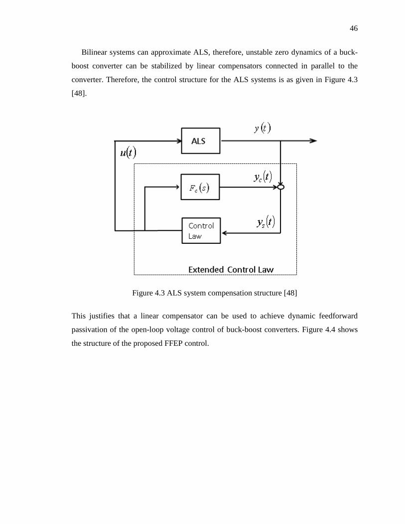
46

Bilinear systems can approximate ALS, therefore, unstable zero dynamics of a buck-

boost converter can be stabilized by linear compensators connected in parallel to the

converter. Therefore, the control structure for the ALS systems is as given in Figure 4.3

[48].

Figure 4.3 ALS system compensation structure [48]

This justifies that a linear compensator can be used to achieve dynamic feedforward

passivation of the open-loop voltage control of buck-boost converters. Figure 4.4 shows

the structure of the proposed FFEP control.

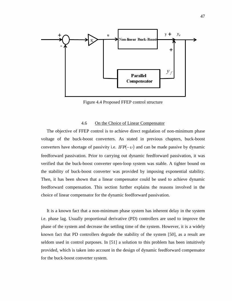
47

Figure 4.4 Proposed FFEP control structure

4.6 On the Choice of Linear Compensator

The objective of FFEP control is to achieve direct regulation of non-minimum phase

voltage of the buck-boost converters. As stated in previous chapters, buck-boost

converters have shortage of passivity i.e. ( )υ−IFP and can be made passive by dynamic

feedforward passivation. Prior to carrying out dynamic feedforward passivation, it was

verified that the buck-boost converter open-loop system was stable. A tighter bound on

the stability of buck-boost converter was provided by imposing exponential stability.

Then, it has been shown that a linear compensator could be used to achieve dynamic

feedforward compensation. This section further explains the reasons involved in the

choice of linear compensator for the dynamic feedforward passivation.

It is a known fact that a non-minimum phase system has inherent delay in the system

i.e. phase lag. Usually proportional derivative (PD) controllers are used to improve the

phase of the system and decrease the settling time of the system. However, it is a widely

known fact that PD controllers degrade the stability of the system [50], as a result are

seldom used in control purposes. In [51] a solution to this problem has been intuitively

provided, which is taken into account in the design of dynamic feedforward compensator

for the buck-boost converter system.

48

[51] states that an effect of a derivative controller of the form,

( )

+=

0

1ssKsH (4.14)

can still be achieved without affecting the stability of the system, by using the inverse of

derivative controller

( )

+

=−

0

1

1ss

DsH (4.15)

where K

D 1= is a feedforward configuration of the system.

Hence, the linear compensator in the design of dynamic feedforward compensation is

considered to be of the form given by

( )1fs

ksG f

−= (4.16)

where 1f is a negative constant, whose state-space description is given as:

ff

fff

zyukzfz

=

+= 1 (4.17)

It is note worth pointing out that the linear compensator is strictly positive real, as the

relative degree is equal to one and the poles and zeros of ( )sG are in the left-half plane.

As ( )sG is strictly positive real, it can be recalled from section 4.3 that ( )sG is passive.

PID controllers are also passive [26], hence ( )sG 1− i.e. the derivative controller is

passive.

The following sections further detail as to how to constrain the gains of the linear

compensator such that the augmented buck-boost converter system becomes and remains

passive.

49

4.7 Lipschitz Continuity

A brief discussion on Lipschitz Continuity is carried out to the constrain the gains of

the linear parallel compensator. A nonlinear system is described by a set of differential

equations. Consider a system given by the following equation:

( ) ( ) 00,, xtxxtfx == (4.18)

The solution to Equation 4.18 with the given initial condition exists and is unique if and

only if the function satisfies the following inequality, called the Lipschitz condition [26]

( ) ( ) yxLytfxtf −≤− ,, (4.19)

where L is called Lipschitz constant. Equation (4.19) can also be written as,

( ) ( ) Lyx

yfxf≤

−−

(4.20)

From the Equation (4.20), it can be said that the derivative of the function f is bounded

by the Lipschitz constant. However, Lipschitz continuity does not imply that the function

f is differentiable.

Lipschitz constant depends on the function. It basically defines how the function f

varies with changes in the input. If f undergoes a large variation for a small change in

input then the function f has a large Lipschitz constant. Therefore, Lipschitz continuity

quantifies the continuity of a function f and Lipschitz constant provides an upper bound

on the amount of variation. The Lipschitz constant of function also depends on the

interval that the function is defined at. If the interval on which the function is defined is

changed, then the Lipschitz constant for the same function is different.

If a function f is defined as RRRf m →×: then the following definition can be given:

50

Definition 4.7: A function f is locally Lipschitz continuous with respect to its first

argument if it is continuous and if for each ( ) RRtx m ×∈, there exists a 0>L such that

( ) ( ) yzLszfsyf −≤− ,, (4.21)

The above definition is used to obtain the Lipschitz constants of the buck-boost converter

system (Equation 4.22)

4.8 Exponential Minimum-phaseness

A system whose zero dynamics are stable is called a minimum phase system. It is

shown in Chapter 2 that the zero dynamics of the buck-boost converter are unstable when

the output of the buck-boost converter system is the voltage across the capacitor. In FFEP

control, the linear compensator (Equation 4.17) in parallel to the buck-boost converter

makes the augmented system passive i.e. dynamic feedforward passivation. From

Theorem 2.1 in Chapter 2, a passive system has relative degree not greater than one and

the zero dynamics are minimum phase. Hence, the gains of the linear compensator are

constrained to make the augmented zero dynamics stable.

Now the normal form of the buck-boost converter is given as:

( ) ( ) ( )( ) ( )( ) ( )

==

+=

tztyzzqtz

uzzbzzatz

1

212

21211

,,,

(4.22)

Where,

( )

( )

( )

−++

−=

−+=

−+−−=

Lz

LzVzC

LCV

RLCzzVzzq

Lz

LzVzC

Czzb

Lzz

LVzC

Cz

RCzza

ininin

in

in

22,

221,

2211,

211

2

211

21

211

221

21

12121

(4.23)

51

Then, the augmented system i.e. the parallel compensator (Equation 4.17) in shunt with

buck-boost converter is represented as

( ) ( )

fa

f

o

f

z

zzy

ub

zbbzfzf

fzz

+=

+

=

1

1

(4.24)

where,

[ ]( ) ( ) ( )[ ][ ]To

Tz

T

b

zqzazf

zzz

01

21

=

=

=

(4.25)

By using the following non-singular co-ordinate transformation,

[ ] ( )fzTT

aa zzz ,φηξ = (4.26)

where

[ ]

( )

22

11

111

21

1

,1

z

ztzbk

z

zzyyz

zz

a

ff

a

ffa

Taaa

aa

=

−=

+=+==

=

η

η

ηηηξ

(4.27)

The normal form of the augmented system is given by

( ) ( )( )( ) ( ) ( )

( )

=

−−=

=

+++==

1

1

2

1

11

,1,1

,

a

ff

ff

a

aa

ffaa

zyzq

ztzbk

zftzbk

za

uktzbzfzazz

ηη

η

ξ

(4.28)

From Equation 4.28 it can be seen that the relative degree of the augmented system is

one. The zero dynamics of the augmented system are obtained by zeroing out the output

011 =+== fa zzzy .

52

Then the zero dynamics aη of the augmented system are given as,

( ) ( ) ( ) ( )[ ]( )

+−

=

==

zq

tzbftzbkz

zaf

f

a

aaa

,,,0 1

2

1

ηη

ηψη (4.29)

The zero dynamics aη can be expressed as,

( ) ( )( )

( )( )

( ) ( ) ( )

( )( ) ( )( )

( ) ( ) ( )2121212

112111211

212121

1121

11211

211

,,,

,1,

,,,

,1

,,

aaaaaa

aaf

aaf

aaaaa

aaf

aaf

aa

qzqq

zzzbk

zzzbkf

azaa

zzzbk

zzzbkfza

ηηηηηη

ηη

ηηηηη

η

ηηη

−+=

−+−

+−+=

−

+−+=

(4.30)

which can be further written as 01 =az

( ) ( ) ( )

( ) ( )

( ) ( )

−

+

−

−

−+=

10

,,

01

,101

,

01

,,

212*1

*12

*1

*12

*1

1

212*1

aaaa

aaaf

aaaf

aaaaaza

qq

bk

bkf

aaf

ηηηη

ηηηηηη

ηηηηηη

(4.31)

where

( ) ( ) ( )]Taaaaaz qaf 2121 ,,[ ηηηηη = (4.32)

and 1*1 za =η as another operating point.

A system (Equation 2.16) is exponentially minimum phase i.e., has exponentially

stable zero dynamics [52] if the Lyapunov energy function of the zero dynamics ( )zVo of

the system satisfy the following relations [25]:

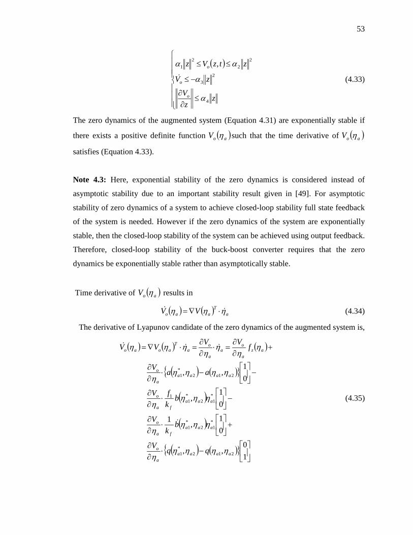
53

( )

≤∂∂

−≤

≤≤

zz

V

zV

ztzVz

o

o

o

4

23

22

21 ,

α

α

αα

(4.33)

The zero dynamics of the augmented system (Equation 4.31) are exponentially stable if

there exists a positive definite function ( )aoV η such that the time derivative of ( )aoV η

satisfies (Equation 4.33).

Note 4.3: Here, exponential stability of the zero dynamics is considered instead of

asymptotic stability due to an important stability result given in [49]. For asymptotic

stability of zero dynamics of a system to achieve closed-loop stability full state feedback

of the system is needed. However if the zero dynamics of the system are exponentially

stable, then the closed-loop stability of the system can be achieved using output feedback.

Therefore, closed-loop stability of the buck-boost converter requires that the zero

dynamics be exponentially stable rather than asymptotically stable.

Time derivative of ( )aoV η results in

( ) ( ) aT

aao VV ηηη ⋅∇= (4.34)

The derivative of Lyapunov candidate of the zero dynamics of the augmented system is,

( ) ( ) ( )

( ) ( )

( )

( )

( ) ( )

−⋅

∂∂

+

⋅

∂∂

−

⋅

∂∂

−

−⋅

∂∂

+∂∂

=⋅∂∂

=⋅∇=

10

,,

01

,1

01

,

01

,,

212*1

*12

*1

*12

*1

1

212*1

aaaaa

o

aaafa

o

aaafa

o

aaaaa

o

aza

oa

a

oa

Taoao

qqV

bk

V

bkfV

aaV

fVVVV

ηηηηη

ηηηη

ηηηη

ηηηηη

ηη

ηη

ηηη

(4.35)

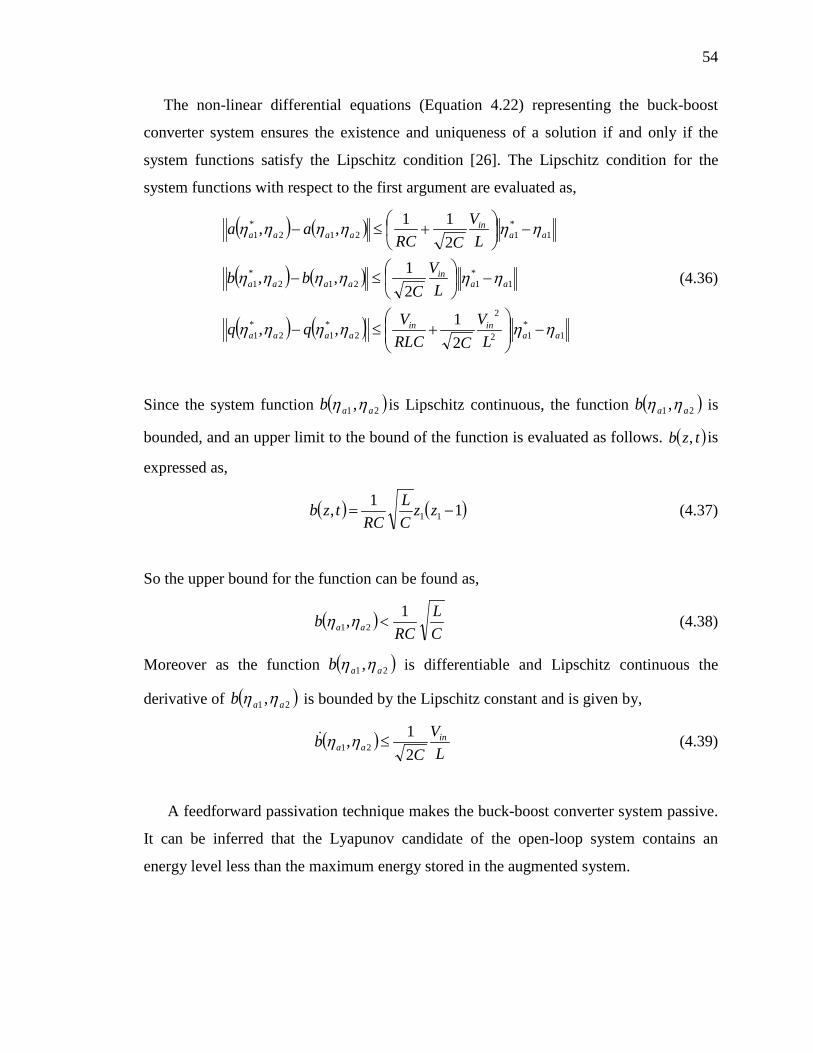
54

The non-linear differential equations (Equation 4.22) representing the buck-boost

converter system ensures the existence and uniqueness of a solution if and only if the

system functions satisfy the Lipschitz condition [26]. The Lipschitz condition for the

system functions with respect to the first argument are evaluated as,

( ) ( )

( ) ( )

( ) ( ) 1*12

2

2*12

*1

1*1212

*1

1*1212

*1

21,,

21,,

211,,

aainin

aaaa

aain

aaaa

aain

aaaa

LV

CRLCVqq

LV

Cbb

LV

CRCaa

ηηηηηη

ηηηηηη

ηηηηηη

−

+≤−

−

≤−

−

+≤−

(4.36)

Since the system function ( )21 , aab ηη is Lipschitz continuous, the function ( )21 , aab ηη is

bounded, and an upper limit to the bound of the function is evaluated as follows. ( )tzb , is

expressed as,

( ) ( )11, 11 −= zzCL

RCtzb (4.37)

So the upper bound for the function can be found as,

( )CL

RCb aa

1, 21 <ηη (4.38)

Moreover as the function ( )21 , aab ηη is differentiable and Lipschitz continuous the

derivative of ( )21 , aab ηη is bounded by the Lipschitz constant and is given by,

( )L

VC

b inaa 2

1, 21 ≤ηη (4.39)

A feedforward passivation technique makes the buck-boost converter system passive.

It can be inferred that the Lyapunov candidate of the open-loop system contains an

energy level less than the maximum energy stored in the augmented system.

55

Therefore, by evaluating the Lipschitz continuity equations and solving Equation 4.35

and using the relations in Equation 4.33 the following relation for the gain constraints of

the parallel compensator are obtained such that the open-loop augmented system is

passive:

1122

+

++> CRC

LRV

LVk inin

f (4.40)

4.9 Closed-Loop Stability

In section 4.8, the detailed procedure to make the augmented buck-boost converter

system passive was outlined. As the control of a passive system can be relatively easy,

the control action is achieved by using a simple proportional gain controller as shown in

Figure 4.4. From Theorem 4.3 and from Note 4.3 the closed-loop stability of buck-boost

converter can be guaranteed.

Theorem 4.3 [24]: If two systems H1 and H2 are passive, then their parallel and

feedback interconnections are also passive.

We can infer that the closed-loop system is passive, where H2 is the positive gain, which

guarantees the closed-loop stability of the system.

4.10 Bias Effect

Application of a parallel interconnection to the buck-boost converter, in dynamic

feedforward passivation, results in a steady state error or bias effect. In order to overcome

the offset in the steady state response, a pre-filter [53] of the following form, is used in

cascade with the plant.

( )δ++

=s

bsasG ff

f (4.41)

where δ,, ff ba are positive constants which satisfy

56

0>−δf

f

ab

(4.42)

Then the structure of the buck-boost converter plant with the pre-filter and a linear

compensator is as given in Figure 4.5.

Now the dynamic feedforward passivation is carried out on the cascade

interconnection of pre-filter and the buck-boost converter. For this to be possible, the

modified buck-boost converter system should be stable i.e. cascade connection of the pre-

filter to buck-boost converter should be stable. This is required because feedforward

passivation cannot influence the stability of the system, recall from Note 4.1. Then the

modified FFEP control structure is given in Figure 4.6.

Figure 4.5 Structure of the plant with pre-filter and linear parallel compensator

Figure 4.6 Modified FFEP control structure

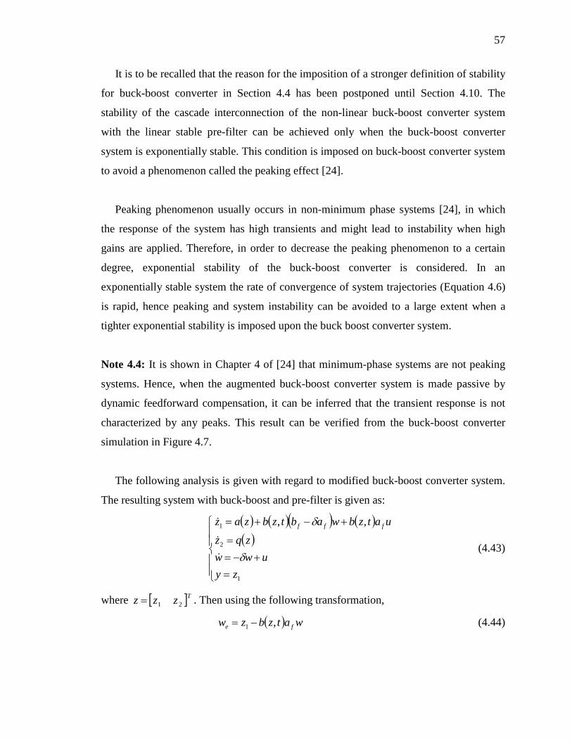
57

It is to be recalled that the reason for the imposition of a stronger definition of stability

for buck-boost converter in Section 4.4 has been postponed until Section 4.10. The

stability of the cascade interconnection of the non-linear buck-boost converter system

with the linear stable pre-filter can be achieved only when the buck-boost converter

system is exponentially stable. This condition is imposed on buck-boost converter system

to avoid a phenomenon called the peaking effect [24].

Peaking phenomenon usually occurs in non-minimum phase systems [24], in which

the response of the system has high transients and might lead to instability when high

gains are applied. Therefore, in order to decrease the peaking phenomenon to a certain

degree, exponential stability of the buck-boost converter is considered. In an

exponentially stable system the rate of convergence of system trajectories (Equation 4.6)

is rapid, hence peaking and system instability can be avoided to a large extent when a

tighter exponential stability is imposed upon the buck boost converter system.

Note 4.4: It is shown in Chapter 4 of [24] that minimum-phase systems are not peaking

systems. Hence, when the augmented buck-boost converter system is made passive by

dynamic feedforward compensation, it can be inferred that the transient response is not

characterized by any peaks. This result can be verified from the buck-boost converter

simulation in Figure 4.7.

The following analysis is given with regard to modified buck-boost converter system.

The resulting system with buck-boost and pre-filter is given as:

( ) ( )( ) ( )( )

=+−=

=

+−+=

1

2

1 ,,

zyuww

zqzuatzbwabtzbzaz fff

δ

δ

(4.43)

where [ ]Tzzz 21= . Then using the following transformation,

( ) watzbzw fe ,1 −= (4.44)

58

the cascaded system is obtained as:

( ) ( )( )( )

===

+=

1

2

1

,

,,

zywzqw

zqzutzbwzaz

eee

eee

(4.45)

where

( ) ( ) ( )

( ) ( )

( ) ( ) ( )( ) ( )

−

−+=

=

−

−+=

ef

fee

fe

ef

fee

wztzbtzb

ab

zawzq

tzbatzb

wzab

zawza

1

1

,,,

,,

,

δ

(4.46)

Then, the augmented system i.e. the parallel compensator (Equation 4.17) in shunt

with buck-boost converter and the pre-filter in cascade is represented as,

( ) ( )

fa

f

o

f

eze

zzy

ub

zbbzfwzf

fzz

+=

+

=

1

1

,

(4.47)

where,

[ ]( ) ( ) ( ) ( )[ ][ ]To

Teeeeez

Te

b

wzqzqwzawzf

wzzz

001

,,,21

=

=

= ε

(4.48)

By using the following non-singular co-ordinate transformation,

[ ] ( )fezTT

aa zzzz ,φηξ ==′ (4.49)

where

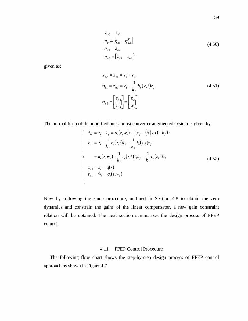
59

[ ]

[ ]Taaa

aa

Taaa

aa

zz

z

zz

432

21

21

1

=

==

=

η

ηηηη

ξ

(4.50)

given as:

( )

=

=

−==

+==

ea

aa

ff

aa

faa

wz

zz

ztzbk

zz

zzzz

2

4

32

121

11

,1

η

η ε

ξ

(4.51)

The normal form of the modified buck-boost converter augmented system is given by:

( ) ( )( )( ) ( )

( ) ( ) ( )

( )( )

====

−−=

−−=

+++=+=

eeea

a

fef

fef

ee

fef

fef

a

fefeefa

wzqwzzqzz

ztzbk

zftzbk

wza

ztzbk

ztzbk

zz

uktzbzfwzazzz

,

,1,1,

,1,1

,,

4

23

1

12

111

(4.52)

Now by following the same procedure, outlined in Section 4.8 to obtain the zero

dynamics and constrain the gains of the linear compensator, a new gain constraint

relation will be obtained. The next section summarizes the design process of FFEP

control.

4.11 FFEP Control Procedure

The following flow chart shows the step-by-step design process of FFEP control

approach as shown in Figure 4.7.

60

Figure 4.7 FFEP control procedure

61

DISCUSSIONS 5.

5.1 Simulations and Experimental Results

This section discusses the simulations and experimental results obtained using FFEP

control approach on buck-boost converter. The FFEP control for direct regulation of

voltage is carried out on a buck-boost converter, simulated using SimPowerSystems

Toolbox in Matlab environment. The following parameters are adopted for buck-boost

converter, resistance Ω= 100R , capacitance FC µ50= , inductance HL µ10= , switching

frequency KHzf s 20= and input voltage .5VVin =

Figure 5.1 shows the voltage regulation profile of the buck-boost converter. It can be

observed that the delay due to over-shoot and under-shoot has been compensated. Figure

5.2 shows the controller effort and Figure 5.3 shows the contribution of the linear

compensator and it can be observed that the bias effect due to the compensator is

negligible. Simulations demonstrate the effectiveness of FFEP control and direct

regulation of non-minimum phase voltage is achieved.

Experiments were also carried out on the buck-boost converter test bed and tested by

implementing the FFEP control using dSPACE rapid-prototyping device. Figure 5.4

shows the voltage regulation profile of the buck-boost converter. The buck-boost

converter test bed is operated at 1 KHz switching frequency and the design parameters of

the test bed are given in the Appendix.

62

Figure 5.1 Voltage regulation profile of converter after FFEP compensation

Figure 5.2 Control effort

0 0.02 0.04 0.06 0.08 0.10

5

10

15

20

Time(Seconds)

Capacitor Voltage x2

0 0.02 0.04 0.06 0.08 0.10

0.2

0.4

0.6

0.8

1Control Effort

Time(Seconds)

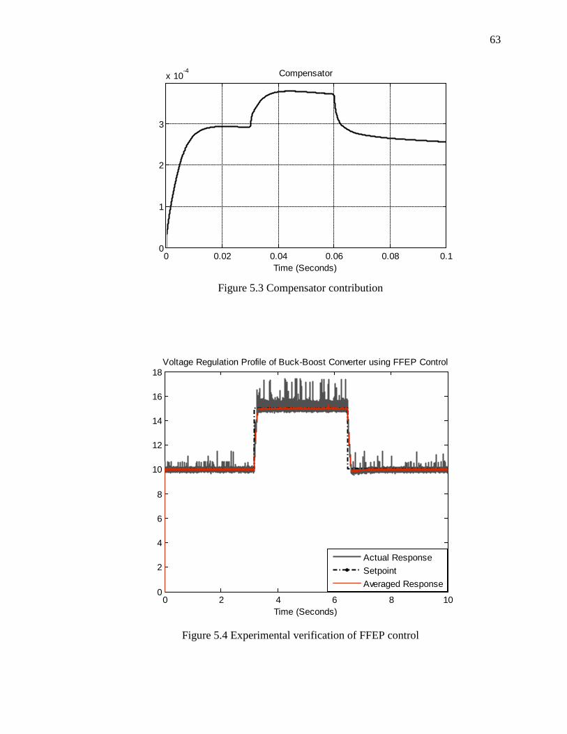
63

Figure 5.3 Compensator contribution

Figure 5.4 Experimental verification of FFEP control

0 0.02 0.04 0.06 0.08 0.10

1

2

3

x 10-4 Compensator

Time (Seconds)

0 2 4 6 8 100

2

4

6

8

10

12

14

16

18

Time (Seconds)

Voltage Regulation Profile of Buck-Boost Converter using FFEP Control

Actual ResponseSetpointAveraged Response

64

5.2 Performance of FFEP Control in the Presence of Load Variations

In the objectives of the thesis it was stated that using FFEP control the sensitivity of

the converter to load variation was reduced significantly. This can be shown by the

following argument. It has been shown in Section 4.4 that the buck-boost converter is IFP

( )υ− by using a general definition for the supply rate. By considering the actual

definition of supply rate given by

( ) ( )22, inin

TT uVxuVuuyuyuw υυ −=−= (5.1)

and

( ) 22

21 2

121 CxLxxS += (5.2)

The following inequalities are obtained,

( ) ( )

( ) 22

22

1

,

xuVuVRxxuV

yuwxS

ininin −<−

<

υ

(5.3)

Then it can be seen by inspection that it is always possible to find a ℜ∈υ , as buck-

boost converter is IFP ( )υ− , such that

( ) υ21 inin uVxuV < (5.4)

and

uRifxuV

Rx

in −<>

11

2

22 (5.5)

The above analysis implies that at high loads (small R), Equation 5.3 holds i.e. the

buck-boost converter has shortage of passivity at high loads or there is insufficient

damping in the system. However, from Chapter 4 in FFEP control dynamic feedforward

passivation is used to make the buck-boost converter system passive. This implies that

irrespective of the load applied to the buck-boost converter system the system is made

passive through dynamic feedforward passivation. Therefore if the load is perturbed, the

system response returns to its nominal behavior as the FFEP control maintains the buck-

boost converter passive through dynamic feedforward passivation.

65

This behavior of the converter in the presence of load variations has been verified using

Simulations. Figure 5.5 and 5.6 shows how the converter returns to its nominal behavior

quickly when the load is decreased by 30% and 50% respectively. Figure 5.7 also shows

the converter’s response when the load is increased by 50%.

Figure 5.5 Response of the converter in the presence of 30% decrease in load

Figure 5.6 Response of the converter in the presence of 50% decrease in load

0 0.02 0.04 0.06 0.08 0.10

5

10

15

Time (Seconds)

Capacitor Voltage x2 ( 30% Perturbation in Load)

R=130 OhmR=100 Ohm

0 0.02 0.04 0.06 0.08 0.10

5

10

15Capacitor Voltage X2 (50% Perturbation in Load)

R=100 Ohm R=150 Ohm

66

Figure 5.7 Response of the converter in the presence of 50% increase in load

Hence, it can be said that FFEP control approach results in a satisfactory performance

when the load varies significantly.

5.3 Comparison of FFEP Control with Other Techniques

In this section FFEP control is compared with different control approaches. In Figure

5.8 a comparison between FFEP and a modified PI control is shown. It can be observed

that even when the gains are fine-tuned, overshoot is observed when a negative step

reference is applied. This attribute cannot be fully eliminated with a PI, as it is due to the

peaking phenomenon [24] inherent in a non-minimum phase system. Therefore, in FFEP

control as the non-minimum phase behavior is compensated to minimum phase by

feedforward passivation, the system behaves close to a minimum phase system. As a

result peaking is very much reduced as can be seen from Figure 5.8.

The FFEP is also compared with other existing passivity based approaches [40, 41]. In

these techniques the energy of the system has been modeled by Hamiltonian [40] and

Brayton - Moser (BM) [41] equations. They constitute the total energy in the system from

0 0.02 0.04 0.06 0.08 0.10

5

10

15Capacitor Voltage X2 (50% Perturbation in Load)

Time (Seconds)

R=100 Ohm R=50 Ohm

67

the internal and external interconnections, and from the damping associated with the

system. In Hamiltonian technique, a closed-loop energy function, the aggregate of the

system, and controller energies is considered. By proper choice of nonlinear control

action and damping injected into the inductor current, [40] achieves the voltage

regulation by driving the closed-loop energy function to a minimum. This technique uses

a state-modulated feedback and a non-quadratic Lyapunov energy function to resolve the

non-minimum phase voltage control. In BM a closed-loop error dynamic function is

considered instead of a closed-loop energy function, and the control task is accomplished

by injecting damping into the capacitor voltage.

Figure 5.8 Comparison of FFEP control with modified PI controller

The principal investigation in [40] and [41] focuses on characterizing the energy of the

system based on the physical structure and makes use of error dynamic and energy

dynamic description to draw conclusions about the degree of passivity i.e. damping in the

0 0.5 1 1.5 2 2.5 30

5

10

15

20

Time (Seconds)

Out

put R

espo

nse

Voltage Regulation Profile with FFEP Control

0 0.5 1 1.5 2 2.5 30

5

10

15

20Voltage Regulation Profile with Modified PI Controller

Out

put R

espo

nse

Time (Seconds)

ResponseReference

Kp:0.3 Ki:1

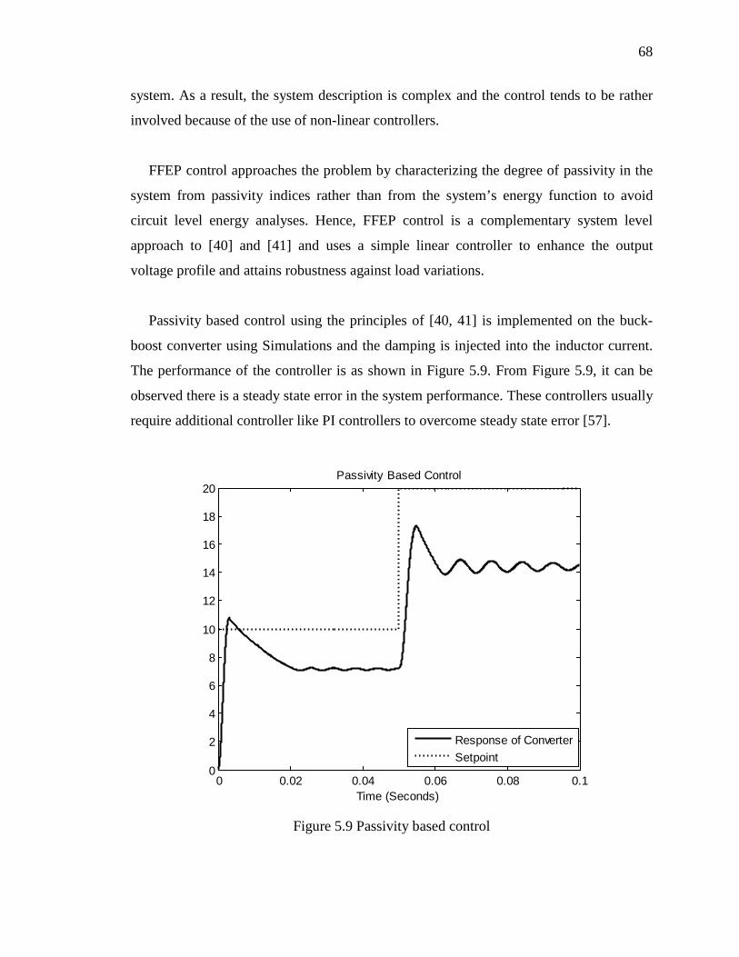
68

system. As a result, the system description is complex and the control tends to be rather

involved because of the use of non-linear controllers.

FFEP control approaches the problem by characterizing the degree of passivity in the

system from passivity indices rather than from the system’s energy function to avoid

circuit level energy analyses. Hence, FFEP control is a complementary system level

approach to [40] and [41] and uses a simple linear controller to enhance the output

voltage profile and attains robustness against load variations.

Passivity based control using the principles of [40, 41] is implemented on the buck-

boost converter using Simulations and the damping is injected into the inductor current.

The performance of the controller is as shown in Figure 5.9. From Figure 5.9, it can be

observed there is a steady state error in the system performance. These controllers usually

require additional controller like PI controllers to overcome steady state error [57].

Figure 5.9 Passivity based control

0 0.02 0.04 0.06 0.08 0.10

2

4

6

8

10

12

14

16

18

20

Time (Seconds)

Passivity Based Control

Response of ConverterSetpoint

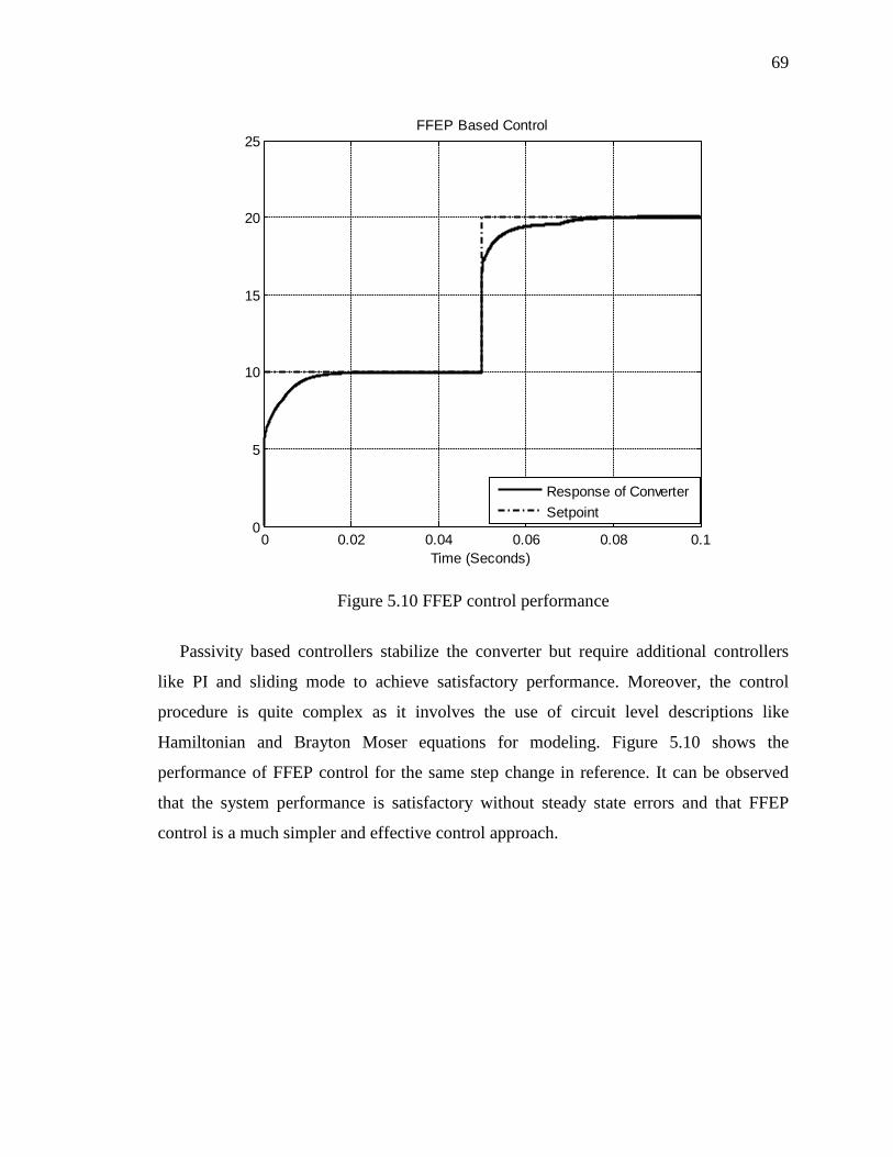
69

Figure 5.10 FFEP control performance

Passivity based controllers stabilize the converter but require additional controllers

like PI and sliding mode to achieve satisfactory performance. Moreover, the control

procedure is quite complex as it involves the use of circuit level descriptions like

Hamiltonian and Brayton Moser equations for modeling. Figure 5.10 shows the

performance of FFEP control for the same step change in reference. It can be observed

that the system performance is satisfactory without steady state errors and that FFEP

control is a much simpler and effective control approach.

0 0.02 0.04 0.06 0.08 0.10

5

10

15

20

25

Time (Seconds)

FFEP Based Control

Response of Converter Setpoint

70

CONCLUSIONS AND RECOMMENDATIONS 6.

6.1 Conclusions

This thesis provided a solution to the problem of direct regulation of non-minimum

phase voltage for second-order DC-DC power converters. Two different methodologies

were introduced depending on the modeling of the converter. For linear converter models,

‘Parallel Compensation Approach [56]’ had been suggested and for bilinear models,

‘Feedforward Excess Passivity (FFEP) based Control’ had been proposed. The main idea

behind these two control approaches is to compensate the non-minimum phase behavior

of the converter such that delay in the system is compensated and a satisfactory

performance of the converter is assured even in the presence of load variations.

In parallel compensation approach, the concept of strictly positive real form of the

system was exploited to achieve a good performance. It has been observed from the

simulation results that the parallel compensation approach accelerates the transient

response of the converter, removes the undershoot and overshoot, considerably reduces

the transient response oscillations and directly controls the voltage. It provided an

alternative solution to the industry standard indirect current mode control. The efficiency

of the control approach has been compared with the conventional proportional integral

controller.

In FFEP based control, a novel system level approach to characterize the damping in

the system has been adopted. The concept of Passivity was used to stabilize the unstable

zero dynamics of the non-minimum phase voltage in the converter. The simulation and

experimental results validate the claim. FFEP based control was also compared with the

existing Passivity based control techniques.

71

Several applications to these control approaches are suggested in the next section,

especially FFEP based control.

6.2 Future Recommendations

This section identifies different problems where FFEP based control can be used as an

effective solution. They are given as:

• Stabilization of constant power loads (CPL) in DC-DC converter systems

• Framework to analyze DC based grid systems

• Model reference adaptive control for non-minimum phase systems

• Solution to overcome peaking effect in non-minimum phase systems

6.2.1 Constant Power Loads

Loads are basically classified into two types: positive incremental loads and negative

incremental loads i.e. constant power loads (CPL). The conventional loads are positive

incremental loads and are usually modeled as resistors, constant current sources, or series

combination of voltage sources, resistors and inductors. Power electronic converters in

multi-converter systems and motor drives exhibit CPL behavior at their input terminals

when they are tightly regulated, as a result the power quality and system stability is

affected. In DC systems, a point of load converters in a multi-converter system behaves

as CPLs and affects the stability of the system.

The voltage and current characteristics of a CPL is as shown in Figure 6.1.and the DC

and small-signal model are given as in Figure 6.2 [54]. The following analysis of buck-

boost converter in the presence of CPL is carried out to show how a stable buck-boost

converter (Equations 2.6 - 2.8) becomes unstable in the presence of a CPL.

72

Figure 6.1 Behavior of constant power loads [CPL]

Figure 6.2 DC and small-signal model of CPL

This scenario usually arises when tightly regulated DC-DC converters acts as loads in

multi-converter system.

The small signal model of the buck-boost converter with CPL is given as:

( ) ( ) ( )( )sd

DLCss

RDL

sDLIVV

DDLCss

RDL

svDDsv

e

Lio

e

io

~

1

1

1

~~

22

222

2

′

+′

−

′−−

′+

′

+′

−′

−= (6.1)

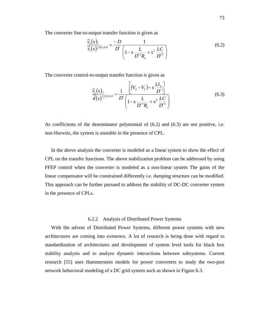
73

The converter line-to-output transfer function is given as

( )( ) ( )

′

+′

−′

−=

=

22

2

0~

1

1~~

DLCs

RDLs

DD

svsv

e

sdi

o (6.2)

The converter control-to-output transfer function is given as

( )( ) ( )

( )

′

+′

−

′−−

′==

22

2

0~

1

1~~

DLCs

RDLs

DLIsVV

Dsdsv

e

LIo

svo

i (6.3)

As coefficients of the denominator polynomial of (6.2) and (6.3) are not positive, i.e.

non-Hurwitz, the system is unstable in the presence of CPL.

In the above analysis the converter is modeled as a linear system to show the effect of

CPL on the transfer functions. The above stabilization problem can be addressed by using

FFEP control when the converter is modeled as a non-linear system The gains of the

linear compensator will be constrained differently i.e. damping structure can be modified.

This approach can be further pursued to address the stability of DC-DC converter system

in the presence of CPLs.

6.2.2 Analysis of Distributed Power Systems

With the advent of Distributed Power Systems, different power systems with new

architectures are coming into existence. A lot of research is being done with regard to

standardization of architectures and development of system level tools for black box

stability analysis and to analyze dynamic interactions between subsystems. Current

research [55] uses Hammerstein models for power converters to study the two-port

network behavioral modeling of a DC grid system such as shown in Figure 6.3.

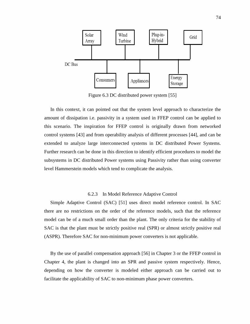
74

Figure 6.3 DC distributed power system [55]

In this context, it can pointed out that the system level approach to characterize the

amount of dissipation i.e. passivity in a system used in FFEP control can be applied to

this scenario. The inspiration for FFEP control is originally drawn from networked

control systems [43] and from operability analysis of different processes [44], and can be

extended to analyze large interconnected systems in DC distributed Power Systems.

Further research can be done in this direction to identify efficient procedures to model the

subsystems in DC distributed Power systems using Passivity rather than using converter

level Hammerstein models which tend to complicate the analysis.

6.2.3 In Model Reference Adaptive Control

Simple Adaptive Control (SAC) [51] uses direct model reference control. In SAC

there are no restrictions on the order of the reference models, such that the reference

model can be of a much small order than the plant. The only criteria for the stability of

SAC is that the plant must be strictly positive real (SPR) or almost strictly positive real

(ASPR). Therefore SAC for non-minimum power converters is not applicable.

By the use of parallel compensation approach [56] in Chapter 3 or the FFEP control in

Chapter 4, the plant is changed into an SPR and passive system respectively. Hence,

depending on how the converter is modeled either approach can be carried out to

facilitate the applicability of SAC to non-minimum phase power converters.

75

6.2.4 In Peaking Phenomenon

From [24] it is said that non-minimum phase systems are peaking systems i.e. they

cannot be stabilized without peaking phenomenon. Such systems when connected in

cascade, in multi-converter system would result in high transients and the system

performance degrades. This can be avoided by the use of FFEP control, as in FFEP

control the system is compensated to make it passive by dynamic feedforward passivation.

Therefore, the system behavior approaches a minimum phase system and the peaking can

be decreased to a considerable effect

LIST OF REFERENCES

76

LIST OF REFERENCES

[1] B. Bryant and M. K. Kazimierezuk, "Derivation of the buck-boost PWM DC-DC converter circuit topology,” IEEE International Symposium on Circuits and Systems, vol. 5, pp. 841-844, 2002.

[2] F. B. Cunha and D. J. Pagano, “Limitations in the control of a DC-DC boost converter,” in Proc. of 15th IFAC World Congress, Barcelona, Spain, 2002.

[3] D. S. Bernstein, "What makes some control problems hard?," IEEE Control Systems Magazine, vol. 22, no. 4, pp. 8-19, Aug 2002.

[4] J. Freudenberg and D. Looze, "Right half plane poles and zeros and design tradeoffs in feedback systems," IEEE Transactions on Automatic Control, vol. 30, no. 6, pp. 555-565, Jun 1985.

[5] R. H. Middleton, “Trade-offs in linear control system design,” Automatica, vol. 27, Issue 2, pp. 281-292, March 1991.

[6] S. Mariéthoz, S. Almér, M. Bâja, A. G. Beccuti, D. Patino, A. Wernrud, J. Buisson, H. Cormerais, T. Geyer, H. Fujioka, U.T. Jönsson, Chung-Yao Kao, M. Morari, G. Papafotiou, A. Rantzer, and P. Riedinger, “Comparison of Hybrid Control Techniques for Buck and Boost DC-DC Converters," IEEE Transactions on Control Systems Technology, vol. 18, no. 5, pp. 1126-1145, Sept. 2010.

[7] J. Alvarez-Ramirez, I. Cervantes, G. Espinosa-Perez, P. Maya, and A. Morales, "A stable design of PI control for DC-DC converters with an RHS zero," IEEE Transactions on Circuits and Systems I: Fundamental Theory and Applications, vol. 48, no. 1, pp. 103-106, Jan 2001.

[8] M. Vidyasagar, "On undershoot and non-minimum phase zeros," IEEE Transactions on Automatic Control, vol. 31, no. 5, pp. 440, May 1986.

77

[9] J. B. Hag and D. S. Bernstein, "Non-minimum-phase zeros - much to do about nothing - classical control - revisited part II," IEEE Control Systems Magazine, vol. 27, no. 3, pp. 45-57, June 2007.

[10] G. Escobar, R. Ortega, H. Sira-Ramirez, J. P. Vilain, and I. Zein, "An experimental comparison of several nonlinear controllers for power converters," IEEE Control Systems, vol. 19, no. 1, pp. 66-82, Feb 1999.

[11] P. T. Krein, J. Bentsman, R. M. Bass, and B. L. Lesieutre, "On the use of averaging for the analysis of power electronic systems," IEEE Transactions on Power Electronics, vol. 5, no. 2, pp. 182-190, Apr 1990.

[12] V. A Caliskan, O. C. Verghese, and A. M. Stankovic, "Multifrequency averaging of DC/DC converters," IEEE Transactions on Power Electronics, vol. 14, no. 1, pp. 124-133, Jan 1999.

[13] S. R. Sanders, J. M. Noworolski, X. Z. Liu, and G. C. Verghese, “Generalized averaging method for power conversion circuits," IEEE Transactions on Power Electronics, vol. 6, no. 2, pp. 251-259, Apr 1991.

[14] J. Mahdavi, A. Emaadi, M. D. Bellar, and M. Ehsani, "Analysis of power electronic converters using the generalized state-space averaging approach," IEEE Transactions on Circuits and Systems I: Fundamental Theory and Applications, vol. 44, no. 8, pp. 767-770, Aug 1997.

[15] R. D. Middlebrook and S. Cuk, “A general unified approach to modeling switching converter power stages,” International Journal of Electronics, vol. 42, pp. 521-550, 1977.

[16] A. J. Forsyth and S. V. Mollov, "Modeling and control of DC-DC converters," Power Engineering Journal, vol. 12, no. 5, pp. 229-236, Oct 1998.

[17] R. W. Erickson and D. Maksimovic, “Fundamentals of Power Electronics,” New York: Chapman & Hill, 1997, p. 261-314.

[18] V. Vorperian, "Simplified analysis of PWM converters using model of PWM switch. Continuous conduction mode," IEEE Transactions on Aerospace and Electronic Systems, vol. 26, no. 3, pp. 490-496, May 1990.

78

[19] Q. Wang, L. Shi, and C. Chang, "Small-signal transfer functions for a single-switch buck-boost converter in continuous conduction mode," 9th International Conference on Solid-State and Integrated-Circuit Technology, pp. 2016-2019, Oct. 2008.

[20] R. R. Mohler,"An Overview of Bilinear System Theory and Applications," IEEE Transactions on Systems, Man and Cybernetics, vol. 10, no. 10, pp. 683-688, Oct. 1980.

[21] L. B. Dunoyer, K. J. Burnham, and D. J. G. James, “Systems modeling and control for industrial plant: a bilinear approach,” in Proceedings of the 13th World Congress of the International Federation of Automatic Control, San Francisco, Calif, USA, June-July 1996.

[22] C. Bruni, G. DiPillo, and G. Koch, "Bilinear systems: An appealing class of nearly linear systems in theory and applications," IEEE Transactions on Automatic Control, vol. 19, no. 4, pp. 334-348, Aug 1974.

[23] A. Isidori. “Nonlinear Control Systems,” Third edition. Springer Verlag, 1995.

[24] R. Sepulchre, M. Jankovic, and P. V. Kokotovic, “Constructive Nonlinear Control,” Springer-Verlag, 1997

[25] J. J. E. Slotine and W. Li, “Applied Nonlinear Control,” Prentice-Hall, 1991.

[26] J. Bao and P. L. Lee, “Process Control,” London: Springer-Verlag, 2007.

[27] R. Lozano-Leal and S. M. Joshi, "Strictly positive real transfer functions revisited," Proceedings of the 29th IEEE Conference on Decision and Control, vol. 6, pp. 3640-3641, Dec 1990.

[28] W. Sun, P. P. Khargonekar, and D. Shim, "Solution to the positive real control problem for linear time-invariant systems," IEEE Transactions on Automatic Control, vol. 39, no. 10, pp. 2034-2046, Oct 1994.

[29] Z. Iwai, I. Mizumoto, and M. Deng, "A parallel feedforward compensator virtually realizing almost strictly positive real plant," Proceedings of the 33rd IEEE Conference on Decision and Control, vol. 3, pp. 2827-2832, Dec 1994.

[30] Z. Iwai, I. Mizumoto, and Y. Nakashima, "Multivariable Stable PID Controller Design with Parallel Feedforward Compensator," International Joint Conference SICE-ICASE, pp. 3246-3251, Oct. 2006.

79

[31] Z. Iwai, I. Mizumoto, L. Liu, S. L. Shah, and H. Jiang, "Adaptive Stable PID Controller with Parallel Feedforward Compensator," 9th International Conference on Control, Automation, Robotics and Vision, pp. 1-6, Dec. 2006.

[32] S. Kahne, "Pole-zero cancellations in SISO linear feedback systems," IEEE Transactions on Education, vol. 33, no. 3, pp. 240-243, Aug 1990.

[33] M. Pradeep, "On the Control of Non-Minimum Phase Systems," American Control Conference, pp. 1295-1296, June 1989.

[34] P. Misra and R. V. Patel, "Transmission zero assignment in linear multivariable systems. I. Square systems," Proceedings of the 27th IEEE Conference on Decision and Control, vol. 2, pp. 1310-1311, Dec 1988.

[35] R. Gessing, "Parallel compensator for control systems with non-minimum phase plants," Proceedings of the American Control Conference 2004, vol. 4, pp. 3351-3356, June 2004-July 2004.

[36] R. Gessing, "Parallel Compensator for Continuous and Relay Control Systems with Difficult Plants," American Control Conference, pp. 5810-5815, July 2007.

[37] K. Lau, R. H. Middleton, and J. H. Braslavsky, "Undershoot and settling time tradeoffs for nonminimum phase systems," IEEE Transactions on Automatic Control , vol. 48, no. 8, pp. 1389-1393, Aug. 2003.

[38] U. Holmberg, P. Mygzkorowski, and R. Longchamp, "On compensation of non-minimum phase zeros,"Automatica, vol. 31, pp. 1433-1441, 1995.

[39] R. Ortega, A. J. Van Der Schaft, I. Mareels, and B. Maschke, "Putting energy back in control," IEEE Control Systems, vol. 21, no. 2, pp. 18-33, Apr 2001.

[40] H. Rodriguez, R. Ortega, and G. Escobar, "A robustly stable output feedback saturated controller for the Boost DC-to-DC converter," Proceedings of the 38th IEEE Conference on Decision and Control, vol. 3, pp. 2100-2105.

[41] D. Jeltsema and J. M. A Scherpen,"Tuning of passivity-preserving controllers for switched-mode power converters,” IEEE Transactions on Automatic Control, vol. 49, no. 8, pp. 1333-1344, Aug. 2004.

[42] T. Shibata and T. Murakami, "Null Space Motion Control by PID Control Considering Passivity in Redundant Manipulator," IEEE Transactions on Industrial Informatics, vol. 4, no. 4, pp. 261-270, Nov. 2008.

80

[43] M. J. McCourt and P. J. Antsaklis, "Stability of networked passive switched systems," 49th IEEE Conference on Decision and Control, pp. 1263-1268, Dec. 2010.

[44] H. Santoso, J. Bao, and P. L. Lee, “Dynamic operability analysis for stable and unstable linear processes,” American Institute of Chemical Engineers Journal, vol. 47, pp. 963-982.

[45] H. Yu and P. J. Antsaklis, "A passivity measure of systems in cascade based on passivity indices," IEEE Conference on Decision and Control, pp. 2186-2191, Dec. 2010.

[46] C. I. Byrnes, A. Isidori, and J. C. Willems, "Passivity, feedback equivalence, and the global stabilization of minimum phase nonlinear systems," IEEE Transactions on Automatic Control, vol. 36, no. 11, pp. 1228-1240, Nov 1991.

[47] G. Palm,"On representation and approximation of nonlinear systems", Biol. Cybern., vol. 34, pp. 49, 1979.

[48] H. Schwarz, “Changing the unstable zero dynamics of nonlinear systems via parallel compensation,” IFAC International Conference on Control, no. 427, pp. 1226-1231, 1996.

[49] C. I. Byrnes and A. Isidori, "Asymptotic stabilization of minimum phase nonlinear systems," IEEE Transactions on Automatic Control, vol. 36, no. 10, pp. 1122-1137, Oct 1991.

[50] K. H. Ang, G. Chong, and Y. Li, "PID control system analysis, design, and technology," IEEE Transactions on Control Systems Technology, vol. 13, no .4, pp. 559- 576, July 2005.

[51] I. Bar-Kana, “Parallel Feedforward and Simplified Adaptive Control,” Int. J. Adaptive Control and Signal Processing, vol. 1, no. 2, pp. 95-109, 1987.

[52] L. Fradkov and D. J. Hill, “Exponential Feedback Passivity and Stabilizability of Nonlinear Systems,” Automatica, vol. 34, no. 6, pp. 697-703, Jun. 1998.

[53] I. Mizumoto, S. Ohishi, and Z. Iwai, "Realization of OFEP-based adaptive output feedback control systems with a PFC," Int. J. of Innovative Computing, Information and Control, vol. 4, no. 12, pp. 3135-3148, 2008.

81

[54] V. Grigore, J. Hatonen, J. Kyyra, and T. Suntio, "Dynamics of a buck converter with a constant power load," Power Electronics Specialists Conference, 1998. PESC 98 Record. 29th Annual IEEE, vol. 1, pp. 72-78, May 1998.

[55] I. Cvetkovic, D. Boroyevich, P. Mattavelli, F. C. Lee, and D. Dong, "Non-linear, hybrid terminal behavioral modeling of a dc-based nanogrid system," Twenty-Sixth Annual IEEE Applied Power Electronics Conference and Exposition (APEC), pp. 1251-1258, March 2011.

[56] L. Gavini, A. Izadian, and L. Li, "A parallel compensation approach in controls of buck-boost converters," 37th Annual Conference on IEEE Industrial Electronics Society, pp. 451-455, Nov. 2011.

[57] B. Wang and Y. Ma, "Research on the passivity-based control strategy of Buck-Boost converters with a wide input power supply range," 2nd IEEE International Symposium on Power Electronics for Distributed Generation Systems, pp. 304-308, June 2010.

APPENDIX

82

APPENDIX

The following figure shows the test bed equipment for buck-boost converter. Figure A.1

shows the dSPACE rapid prototyping device, buck-boost converter and a programmable

load.

Figure A Buck-Boost Converter Experimental Setup

.