GradNorm: Gradient Normalization for Adaptive Loss Balancing in … · 2018-06-13 · GradNorm: Gradient Normalization for Adaptive Loss Balancing in Deep Multitask Networks Zhao

GradNorm: Gradient Normalization for AdaptiveLoss Balancing in Deep Multitask Networks

Zhao Chen 1 Vijay Badrinarayanan 1 Chen-Yu Lee 1 Andrew Rabinovich 1

AbstractDeep multitask networks, in which one neural net-work produces multiple predictive outputs, canoffer better speed and performance than theirsingle-task counterparts but are challenging totrain properly. We present a gradient normaliza-tion (GradNorm) algorithm that automatically bal-ances training in deep multitask models by dynam-ically tuning gradient magnitudes. We show thatfor various network architectures, for both regres-sion and classification tasks, and on both syntheticand real datasets, GradNorm improves accuracyand reduces overfitting across multiple tasks whencompared to single-task networks, static baselines,and other adaptive multitask loss balancing tech-niques. GradNorm also matches or surpasses theperformance of exhaustive grid search methods,despite only involving a single asymmetry hy-perparameter α. Thus, what was once a tedioussearch process that incurred exponentially morecompute for each task added can now be accom-plished within a few training runs, irrespective ofthe number of tasks. Ultimately, we will demon-strate that gradient manipulation affords us greatcontrol over the training dynamics of multitasknetworks and may be one of the keys to unlockingthe potential of multitask learning.

1. IntroductionSingle-task learning in computer vision has enjoyed muchsuccess in deep learning, with many single-task models nowperforming at or beyond human accuracies for a wide arrayof tasks. However, an ultimate visual system for full sceneunderstanding must be able to perform many diverse percep-tual tasks simultaneously and efficiently, especially withinthe limited compute environments of embedded systems

1Magic Leap, Inc. Correspondence to: Zhao Chen<[email protected]>.

Proceedings of the 35 th International Conference on MachineLearning, Stockholm, Sweden, PMLR 80, 2018. Copyright 2018by the author(s).

such as smartphones, wearable devices, and robots/drones.Such a system can be enabled by multitask learning, whereone model shares weights across multiple tasks and makesmultiple inferences in one forward pass. Such networksare not only scalable, but the shared features within thesenetworks can induce more robust regularization and boostperformance as a result. In the ideal limit, we can thushave the best of both worlds with multitask networks: moreefficiency and higher performance.

In general, multitask networks are difficult to train; differenttasks need to be properly balanced so network parametersconverge to robust shared features that are useful across alltasks. Methods in multitask learning thus far have largelytried to find this balance by manipulating the forward passof the network (e.g. through constructing explicit statisti-cal relationships between features (Long & Wang, 2015)or optimizing multitask network architectures (Misra et al.,2016), etc.), but such methods ignore a key insight: taskimbalances impede proper training because they manifestas imbalances between backpropagated gradients. A taskthat is too dominant during training, for example, will neces-sarily express that dominance by inducing gradients whichhave relatively large magnitudes. We aim to mitigate such is-sues at their root by directly modifying gradient magnitudesthrough tuning of the multitask loss function.

In practice, the multitask loss function is often assumed tobe linear in the single task losses Li, L =

∑i wiLi, where

the sum runs over all T tasks. In our case, we propose anadaptive method, and so wi can vary at each training stept: wi = wi(t). This linear form of the loss function isconvenient for implementing gradient balancing, as wi verydirectly and linearly couples to the backpropagated gradientmagnitudes from each task. The challenge is then to find thebest value for each wi at each training step t that balancesthe contribution of each task for optimal model training.To optimize the weights wi(t) for gradient balancing, wepropose a simple algorithm that penalizes the network whenbackpropagated gradients from any task are too large or toosmall. The correct balance is struck when tasks are train-ing at similar rates; if task i is training relatively quickly,then its weight wi(t) should decrease relative to other taskweights wj(t)|j 6=i to allow other tasks more influence on

arX

iv:1

711.

0225

7v4

[cs

.CV

] 1

2 Ju

n 20

18

GradNorm: Gradient Normalization for Adaptive Loss Balancing in Deep Multitask Networks

training. Our algorithm is similar to batch normalization(Ioffe & Szegedy, 2015) with two main differences: (1) wenormalize across tasks instead of across data batches, and(2) we use rate balancing as a desired objective to informour normalization. We will show that such gradient normal-ization (hereafter referred to as GradNorm) boosts networkperformance while significantly curtailing overfitting.

Our main contributions to multitask learning are as follows:

1. An efficient algorithm for multitask loss balancingwhich directly tunes gradient magnitudes.

2. A method which matches or surpasses the performanceof very expensive exhaustive grid search procedures,but which only requires tuning a single hyperparameter.

3. A demonstration that direct gradient interaction pro-vides a powerful way of controlling multitask learning.

2. Related WorkMultitask learning was introduced well before the advent ofdeep learning (Caruana, 1998; Bakker & Heskes, 2003), butthe robust learned features within deep networks and theirexcellent single-task performance have spurned renewedinterest. Although our primary application area is computervision, multitask learning has applications in multiple otherfields, from natural language processing (Collobert & We-ston, 2008; Hashimoto et al., 2016; Søgaard & Goldberg,2016) to speech synthesis (Seltzer & Droppo, 2013; Wuet al., 2015), from very domain-specific applications suchas traffic prediction (Huang et al., 2014) to very generalcross-domain work (Bilen & Vedaldi, 2017). Multitasklearning has also been explored in the context of curriculumlearning (Graves et al., 2017), where subsets of tasks aresubsequently trained based on local rewards; we here ex-plore the opposite approach, where tasks are jointly trainedbased on global rewards such as total loss decrease.

Multitask learning is very well-suited to the field of com-puter vision, where making multiple robust predictions iscrucial for complete scene understanding. Deep networkshave been used to solve various subsets of multiple visiontasks, from 3-task networks (Eigen & Fergus, 2015; Te-ichmann et al., 2016) to much larger subsets as in Uber-Net (Kokkinos, 2016). Often, single computer vision prob-lems can even be framed as multitask problems, such as inMask R-CNN for instance segmentation (He et al., 2017) orYOLO-9000 for object detection (Redmon & Farhadi, 2016).Particularly of note is the rich and significant body of workon finding explicit ways to exploit task relationships withina multitask model. Clustering methods have shown successbeyond deep models (Jacob et al., 2009; Kang et al., 2011),while constructs such as deep relationship networks (Long& Wang, 2015) and cross-stich networks (Misra et al., 2016)

give deep networks the capacity to search for meaningfulrelationships between tasks and to learn which features toshare between them. Work in (Warde-Farley et al., 2014)and (Lu et al., 2016) use groupings amongst labels to searchthrough possible architectures for learning. Perhaps themost relevant to the current work, (Kendall et al., 2017) usesa joint likelihood formulation to derive task weights basedon the intrinsic uncertainty in each task.

3. The GradNorm Algorithm3.1. Definitions and Preliminaries

For a multitask loss function L(t) =∑wi(t)Li(t), we aim

to learn the functions wi(t) with the following goals: (1)to place gradient norms for different tasks on a commonscale through which we can reason about their relative mag-nitudes, and (2) to dynamically adjust gradient norms sodifferent tasks train at similar rates. To this end, we first de-fine the relevant quantities, first with respect to the gradientswe will be manipulating.

• W : The subset of the full network weights W ⊂ Wwhere we actually apply GradNorm. W is generallychosen as the last shared layer of weights to save oncompute costs1.

• G(i)W (t) = ||∇Wwi(t)Li(t)||2: the L2 norm of the

gradient of the weighted single-task loss wi(t)Li(t)with respect to the chosen weights W .

• GW (t) = Etask[G(i)W (t)]: the average gradient norm

across all tasks at training time t.

We also define various training rates for each task i:

• Li(t) = Li(t)/Li(0): the loss ratio for task i at timet. Li(t) is a measure of the inverse training rate oftask i (i.e. lower values of Li(t) correspond to a fastertraining rate for task i)2.

• ri(t) = Li(t)/Etask[Li(t)]: the relative inverse train-ing rate of task i.

With the above definitions in place, we now complete ourdescription of the GradNorm algorithm.

3.2. Balancing Gradients with GradNorm

As stated in Section 3.1, GradNorm should establish a com-mon scale for gradient magnitudes, and also should balance

1In our experiments this choice of W causes GradNorm toincrease training time by only ∼ 5% on NYUv2.

2Networks in this paper all had stable initializations and Li(0)could be used directly. When Li(0) is sharply dependent on ini-tialization, we can use a theoretical initial loss instead. E.g. for Li

the CE loss across C classes, we can use Li(0) = log(C).


Figure 1. Gradient Normalization. Imbalanced gradient norms across tasks (left) result in suboptimal training within a multitask network.We implement GradNorm through computing a novel gradient loss Lgrad (right) which tunes the loss weights wi to fix such imbalances ingradient norms. We illustrate here a simplified case where such balancing results in equalized gradient norms, but in general there may betasks that require relatively high or low gradient magnitudes for optimal training (discussed further in Section 3).

training rates of different tasks. The common scale for gra-dients is most naturally the average gradient norm, GW (t),which establishes a baseline at each timestep t by which wecan determine relative gradient sizes. The relative inversetraining rate of task i, ri(t), can be used to rate balanceour gradients. Concretely, the higher the value of ri(t), thehigher the gradient magnitudes should be for task i in orderto encourage the task to train more quickly. Therefore, ourdesired gradient norm for each task i is simply:

G(i)W (t) 7→ GW (t)× [ri(t)]

α, (1)

where α is an additional hyperparameter. α sets the strengthof the restoring force which pulls tasks back to a commontraining rate. In cases where tasks are very different intheir complexity, leading to dramatically different learningdynamics between tasks, a higher value of α should be usedto enforce stronger training rate balancing. When tasks aremore symmetric (e.g. the synthetic examples in Section 4),a lower value of α is appropriate. Note that α = 0 willalways try to pin the norms of backpropagated gradientsfrom each task to be equal at W . See Section 5.4 for moredetails on the effects of tuning α.

Equation 1 gives a target for each task i’s gradient norms,and we update our loss weights wi(t) to move gradient

norms towards this target for each task. GradNorm is thenimplemented as an L1 loss function Lgrad between the actualand target gradient norms at each timestep for each task,summed over all tasks:

Lgrad(t;wi(t)) =∑i

∣∣∣∣G(i)W (t)−GW (t)× [ri(t)]

α

∣∣∣∣1

(2)

where the summation runs through all T tasks. When dif-ferentiating this loss Lgrad, we treat the target gradient normGW (t)× [ri(t)]

α as a fixed constant to prevent loss weightswi(t) from spuriously drifting towards zero. Lgrad is thendifferentiated only with respect to the wi, as the wi(t) di-rectly control gradient magnitudes per task. The computedgradients ∇wi

Lgrad are then applied via standard updaterules to update each wi (as shown in Figure 1). The fullGradNorm algorithm is summarized in Algorithm 1. Notethat after every update step, we also renormalize the weightswi(t) so that

∑i wi(t) = T in order to decouple gradient

normalization from the global learning rate.

4. A Toy ExampleTo illustrate GradNorm on a simple, interpretable system,we construct a common scenario for multitask networks:training tasks which have similar loss functions but differentloss scales. In such situations, if we naıvely pick wi(t) = 1


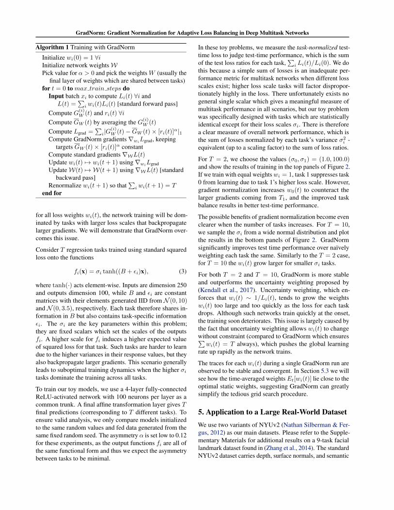
Algorithm 1 Training with GradNorm

Initialize wi(0) = 1 ∀iInitialize network weightsWPick value for α > 0 and pick the weightsW (usually the

final layer of weights which are shared between tasks)for t = 0 to max train steps do

Input batch xi to compute Li(t) ∀i andL(t) =

∑i wi(t)Li(t) [standard forward pass]

Compute G(i)W (t) and ri(t) ∀i

Compute GW (t) by averaging the G(i)W (t)

Compute Lgrad =∑i|G

(i)W (t)−GW (t)× [ri(t)]

α|1Compute GradNorm gradients∇wi

Lgrad, keepingtargets GW (t)× [ri(t)]

α constantCompute standard gradients∇WL(t)Update wi(t) 7→ wi(t+ 1) using ∇wiLgradUpdateW(t) 7→ W(t+ 1) using∇WL(t) [standard

backward pass]Renormalize wi(t+ 1) so that

∑i wi(t+ 1) = T

end for

for all loss weights wi(t), the network training will be dom-inated by tasks with larger loss scales that backpropagatelarger gradients. We will demonstrate that GradNorm over-comes this issue.

Consider T regression tasks trained using standard squaredloss onto the functions

fi(x) = σi tanh((B + εi)x), (3)

where tanh(·) acts element-wise. Inputs are dimension 250and outputs dimension 100, while B and εi are constantmatrices with their elements generated IID from N (0, 10)and N (0, 3.5), respectively. Each task therefore shares in-formation in B but also contains task-specific informationεi. The σi are the key parameters within this problem;they are fixed scalars which set the scales of the outputsfi. A higher scale for fi induces a higher expected valueof squared loss for that task. Such tasks are harder to learndue to the higher variances in their response values, but theyalso backpropagate larger gradients. This scenario generallyleads to suboptimal training dynamics when the higher σitasks dominate the training across all tasks.

To train our toy models, we use a 4-layer fully-connectedReLU-activated network with 100 neurons per layer as acommon trunk. A final affine transformation layer gives Tfinal predictions (corresponding to T different tasks). Toensure valid analysis, we only compare models initializedto the same random values and fed data generated from thesame fixed random seed. The asymmetry α is set low to 0.12for these experiments, as the output functions fi are all ofthe same functional form and thus we expect the asymmetrybetween tasks to be minimal.

In these toy problems, we measure the task-normalized test-time loss to judge test-time performance, which is the sumof the test loss ratios for each task,

∑i Li(t)/Li(0). We do

this because a simple sum of losses is an inadequate per-formance metric for multitask networks when different lossscales exist; higher loss scale tasks will factor dispropor-tionately highly in the loss. There unfortunately exists nogeneral single scalar which gives a meaningful measure ofmultitask performance in all scenarios, but our toy problemwas specifically designed with tasks which are statisticallyidentical except for their loss scales σi. There is thereforea clear measure of overall network performance, which isthe sum of losses normalized by each task’s variance σ2

i -equivalent (up to a scaling factor) to the sum of loss ratios.

For T = 2, we choose the values (σ0, σ1) = (1.0, 100.0)and show the results of training in the top panels of Figure 2.If we train with equal weightswi = 1, task 1 suppresses task0 from learning due to task 1’s higher loss scale. However,gradient normalization increases w0(t) to counteract thelarger gradients coming from T1, and the improved taskbalance results in better test-time performance.

The possible benefits of gradient normalization become evenclearer when the number of tasks increases. For T = 10,we sample the σi from a wide normal distribution and plotthe results in the bottom panels of Figure 2. GradNormsignificantly improves test time performance over naıvelyweighting each task the same. Similarly to the T = 2 case,for T = 10 the wi(t) grow larger for smaller σi tasks.

For both T = 2 and T = 10, GradNorm is more stableand outperforms the uncertainty weighting proposed by(Kendall et al., 2017). Uncertainty weighting, which en-forces that wi(t) ∼ 1/Li(t), tends to grow the weightswi(t) too large and too quickly as the loss for each taskdrops. Although such networks train quickly at the onset,the training soon deteriorates. This issue is largely caused bythe fact that uncertainty weighting allows wi(t) to changewithout constraint (compared to GradNorm which ensures∑wi(t) = T always), which pushes the global learning

rate up rapidly as the network trains.

The traces for each wi(t) during a single GradNorm run areobserved to be stable and convergent. In Section 5.3 we willsee how the time-averaged weightsEt[wi(t)] lie close to theoptimal static weights, suggesting GradNorm can greatlysimplify the tedious grid search procedure.

5. Application to a Large Real-World DatasetWe use two variants of NYUv2 (Nathan Silberman & Fer-gus, 2012) as our main datasets. Please refer to the Supple-mentary Materials for additional results on a 9-task faciallandmark dataset found in (Zhang et al., 2014). The standardNYUv2 dataset carries depth, surface normals, and semantic


Figure 2. Gradient Normalization on a toy 2-task (top) and 10-task (bottom) system. Diagrams of the network structure with lossscales are on the left, traces of wi(t) during training in the middle, and task-normalized test loss curves on the right. α = 0.12 for all runs.

segmentation labels (clustered into 13 distinct classes) for avariety of indoor scenes in different room types (bathrooms,living rooms, studies, etc.). NYUv2 is relatively small (795training, 654 test images), but contains both regression andclassification labels, making it a good choice to test therobustness of GradNorm across various tasks.

We augment the standard NYUv2 depth dataset with flipsand additional frames from each video, resulting in 90,000images complete with pixel-wise depth, surface normals,and room keypoint labels (segmentation labels are, unfortu-nately, not available for these additional frames). Keypointlabels are professionally annotated by humans, while sur-face normals are generated algorithmically. The full datasetis then split by scene for a 90/10 train/test split. See Figure6 for examples. We will generally refer to these two datasetsas NYUv2+seg and NYUv2+kpts, respectively.

All inputs are downsampled to 320 x 320 pixels and outputsto 80 x 80 pixels. We use these resolutions following (Leeet al., 2017), which represents the state-of-the-art in roomkeypoint prediction and from which we also derive ourVGG-style model architecture. These resolutions also allowus to keep models relatively slim while not compromisingsemantic complexity in the ground truth output maps.

5.1. Model and General Training Characteristics

We try two different models: (1) a SegNet (Badrinarayananet al., 2015; Lee et al., 2017) network with a symmetricVGG16 (Simonyan & Zisserman, 2014) encoder/decoder,

and (2) an FCN (Long et al., 2015) network with a modifiedResNet-50 (He et al., 2016) encoder and shallow ResNet de-coder. The VGG SegNet reuses maxpool indices to performupsampling, while the ResNet FCN learns all upsamplingfilters. The ResNet architecture is further thinned (both inits filters and activations) to contrast with the heavier, morecomplex VGG SegNet: stride-2 layers are moved earlierand all 2048-filter layers are replaced by 1024-filter layers.Ultimately, the VGG SegNet has 29M parameters versus15M for the thin ResNet. All model parameters are sharedamongst all tasks until the final layer. Although we willfocus on the VGG SegNet in our more in-depth analysis,by designing and testing on two extremely different net-work topologies we will further demonstrate GradNorm’srobustness to the choice of base architecture.

We use standard pixel-wise loss functions for each task:cross entropy for segmentation, squared loss for depth, andcosine similarity for normals. As in (Lee et al., 2017), forroom layout we generate Gaussian heatmaps for each of48 room keypoint types and predict these heatmaps witha pixel-wise squared loss. Note that all regression tasksare quadratic losses (our surface normal prediction uses acosine loss which is quadratic to leading order), allowing usto use ri(t) for each task i as a direct proxy for each task’srelative inverse training rate.

All runs are trained at a batch size of 24 across 4 TitanX GTX 12GB GPUs and run at 30fps on a single GPU atinference. All NYUv2 runs begin with a learning rate of 2e-5. NYUv2+kpts runs last 80000 steps with a learning rate


Table 1. Test error, NYUv2+seg for GradNorm and various base-lines. Lower values are better. Best performance for each task isbolded, with second-best underlined.

Model and Depth Seg. NormalsWeighting RMS Err. Err. Err.

Method (m) (100-IoU) (1-|cos|)VGG Backbone

Depth Only 1.038 - -Seg. Only - 70.0 -

Normals Only - - 0.169Equal Weights 0.944 70.1 0.192

GradNorm Static 0.939 67.5 0.171GradNorm α = 1.5 0.925 67.8 0.174

decay of 0.2 every 25000 steps. NYUv2+seg runs last 20000steps with a learning rate decay of 0.2 every 6000 steps.Updating wi(t) is performed at a learning rate of 0.025 forboth GradNorm and the uncertainty weighting ((Kendallet al., 2017)) baseline. All optimizers are Adam, althoughwe find that GradNorm is insensitive to the optimizer chosen.We implement GradNorm using TensorFlow v1.2.1.

5.2. Main Results on NYUv2

In Table 1 we display the performance of GradNorm onthe NYUv2+seg dataset. We see that GradNorm α = 1.5improves the performance of all three tasks with respectto the equal-weights baseline (where wi(t) = 1 for all t,i),and either surpasses or matches (within statistical noise)the best performance of single networks for each task.The GradNorm Static network uses static weights derivedfrom a GradNorm network by calculating the time-averagedweights Et[wi(t)] for each task during a GradNorm trainingrun, and retraining a network with weights fixed to thosevalues. GradNorm thus can also be used to extract goodvalues for static weights. We pursue this idea further inSection 5.3 and show that these weights lie very close to theoptimal weights extracted from exhaustive grid search.

To show how GradNorm can perform in the presence of alarger dataset, we also perform extensive experiments onthe NYUv2+kpts dataset, which is augmented to a factorof 50x more data. The results are shown in Table 2. Aswith the NYUv2+seg runs, GradNorm networks outperformother multitask methods, and either matches (within noise)or surpasses the performance of single-task networks.

Figure 3 shows test and training loss curves for GradNorm(α = 1.5) and baselines on the larger NYUv2+kpts datasetfor our VGG SegNet models. GradNorm improves test-timedepth error by ∼ 5%, despite converging to a much highertraining loss. GradNorm achieves this by aggressively ratebalancing the network (enforced by a high asymmetry α =1.5), and ultimately suppresses the depth weight wdepth(t) tolower than 0.10 (see Section 5.4 for more details). The same

Figure 3. Test and training loss curves for all tasks inNYUv2+kpts, VGG16 backbone. GradNorm versus an equalweights baseline and uncertainty weighting (Kendall et al., 2017).

trend exists for keypoint regression, and is a clear signal ofnetwork regularization. In contrast, uncertainty weighting(Kendall et al., 2017) always moves test and training error inthe same direction, and thus is not a good regularizer. Onlyresults for the VGG SegNet are shown here, but the ThinResNet FCN produces consistent results.

5.3. Gradient Normalization Finds OptimalGrid-Search Weights in One Pass

For our VGG SegNet, we train 100 networks from scratchwith random task weights on NYUv2+kpts. Weights aresampled from a uniform distribution and renormalized tosum to T = 3. For computational efficiency, we only trainfor 15000 iterations out of the normal 80000, and thencompare the performance of that network to our GradNorm


Table 2. Test error, NYUv2+kpts for GradNorm and various base-lines. Lower values are better. Best performance for each task isbolded, with second-best underlined.

Model and Depth Kpt. NormalsWeighting RMS Err. Err. Err.

Method (m) (%) (1-|cos|)ResNet Backbone

Depth Only 0.725 - -Kpt Only - 7.90 -

Normals Only - - 0.155Equal Weights 0.697 7.80 0.172

(Kendall et al., 2017) 0.702 7.96 0.182GradNorm Static 0.695 7.63 0.156

GradNorm α = 1.5 0.663 7.32 0.155VGG Backbone

Depth Only 0.689 - -Keypoint Only - 8.39 -Normals Only - - 0.142Equal Weights 0.658 8.39 0.155

(Kendall et al., 2017) 0.649 8.00 0.158GradNorm Static 0.638 7.69 0.137

GradNorm α = 1.5 0.629 7.73 0.139

Figure 4. Gridsearch performance for random task weightsvs GradNorm, NYUv2+kpts. Average change in performanceacross three tasks for a static multitask network with weightswstatic

i ,plotted against the L2 distance between wstatic

i and a set of staticweights derived from a GradNorm network, Et[wi(t)]. A refer-ence line at zero performance change is provided for convenience.All comparisons are made at 15000 steps of training.

α = 1.5 VGG SegNet network at the same 15000 steps.The results are shown in Figure 4.

Even after 100 networks trained, grid search still falls shortof our GradNorm network. Even more remarkably, there isa strong, negative correlation between network performanceand task weight distance to our time-averaged GradNormweights Et[wi(t)]. At an L2 distance of ∼ 3, grid searchnetworks on average have almost double the errors per taskcompared to our GradNorm network. GradNorm has there-fore found the optimal grid search weights in one singletraining run.

Figure 5. Weights wi(t) during training, NYUv2+kpts. Tracesof how the task weights wi(t) change during training for twodifferent values of α. A larger value of α pushes weights fartherapart, leading to less symmetry between tasks.

5.4. Effects of tuning the asymmetry α

The only hyperparameter in our algorithm is the asymmetryα. The optimal value of α for NYUv2 lies near α = 1.5,while in the highly symmetric toy example in Section 4 weused α = 0.12. This observation reinforces our characteri-zation of α as an asymmetry parameter.

Tuning α leads to performance gains, but we found thatfor NYUv2, almost any value of 0 < α < 3 will improvenetwork performance over an equal weights baseline (seeSupplementary for details). Figure 5 shows that higher val-ues of α tend to push the weights wi(t) further apart, whichmore aggressively reduces the influence of tasks which over-fit or learn too quickly (in our case, depth). Remarkably, atα = 1.75 (not shown) wdepth(t) is suppressed to below 0.02at no detriment to network performance on the depth task.

5.5. Qualitative Results

Figure 6 shows visualizations of the VGG SegNet outputson test set images along with the ground truth, for both theNYUv2+seg and NYUv2+kpts datasets. Ground truth labelsare juxtaposed with outputs from the equal weights network,3 single networks, and our best GradNorm network. Some


Figure 6. Visualizations at inference time. NYUv2+kpts outputs are shown on the left, while NYUv2+seg outputs are shown on theright. Visualizations shown were generated from random test set images. Some improvements are incremental, but red frames are drawnaround predictions that are visually more clearly improved by GradNorm. For NYUv2+kpts outputs GradNorm shows improvementover the equal weights network in normals prediction and over single networks in keypoint prediction. For NYUv2+seg there is animprovement over single networks in depth and segmentation accuracy. These are consistent with the numbers reported in Tables 1 and 2.

improvements are incremental, but GradNorm producessuperior visual results in tasks for which there are significantquantitative improvements in Tables 1 and 2.

6. ConclusionsWe introduced GradNorm, an efficient algorithm for tun-ing loss weights in a multi-task learning setting based onbalancing the training rates of different tasks. We demon-strated on both synthetic and real datasets that GradNormimproves multitask test-time performance in a variety ofscenarios, and can accommodate various levels of asymme-try amongst the different tasks through the hyperparameterα. Our empirical results indicate that GradNorm offers su-

perior performance over state-of-the-art multitask adaptiveweighting methods and can match or surpass the perfor-mance of exhaustive grid search while being significantlyless time-intensive.

Looking ahead, algorithms such as GradNorm may haveapplications beyond multitask learning. We hope to extendthe GradNorm approach to work with class-balancing andsequence-to-sequence models, all situations where problemswith conflicting gradient signals can degrade model perfor-mance. We thus believe that our work not only provides arobust new algorithm for multitask learning, but also rein-forces the powerful idea that gradient tuning is fundamentalfor training large, effective models on complex tasks.


ReferencesBadrinarayanan, V., Kendall, A., and Cipolla, R. Segnet:

A deep convolutional encoder-decoder architecture forimage segmentation. arXiv preprint arXiv:1511.00561,2015.

Bakker, B. and Heskes, T. Task clustering and gating forbayesian multitask learning. Journal of Machine Learn-ing Research, 4(May):83–99, 2003.

Bilen, H. and Vedaldi, A. Universal representations: Themissing link between faces, text, planktons, and catbreeds. arXiv preprint arXiv:1701.07275, 2017.

Caruana, R. Multitask learning. In Learning to learn, pp.95–133. Springer, 1998.

Collobert, R. and Weston, J. A unified architecture for natu-ral language processing: Deep neural networks with mul-titask learning. In Proceedings of the 25th internationalconference on Machine learning, pp. 160–167. ACM,2008.

Eigen, D. and Fergus, R. Predicting depth, surface normalsand semantic labels with a common multi-scale convolu-tional architecture. In Proceedings of the IEEE Interna-tional Conference on Computer Vision, pp. 2650–2658,2015.

Graves, A., Bellemare, M. G., Menick, J., Munos, R., andKavukcuoglu, K. Automated curriculum learning forneural networks. arXiv preprint arXiv:1704.03003, 2017.

Hashimoto, K., Xiong, C., Tsuruoka, Y., and Socher, R. Ajoint many-task model: Growing a neural network formultiple nlp tasks. arXiv preprint arXiv:1611.01587,2016.

He, K., Zhang, X., Ren, S., and Sun, J. Deep residual learn-ing for image recognition. In Proceedings of the IEEEconference on computer vision and pattern recognition,pp. 770–778, 2016.

He, K., Gkioxari, G., Dollar, P., and Girshick, R. Maskr-cnn. arXiv preprint arXiv:1703.06870, 2017.

Huang, W., Song, G., Hong, H., and Xie, K. Deep archi-tecture for traffic flow prediction: deep belief networkswith multitask learning. IEEE Transactions on IntelligentTransportation Systems, 15(5):2191–2201, 2014.

Ioffe, S. and Szegedy, C. Batch normalization: Acceleratingdeep network training by reducing internal covariate shift.In International Conference on Machine Learning, pp.448–456, 2015.

Jacob, L., Vert, J.-p., and Bach, F. R. Clustered multi-tasklearning: A convex formulation. In Advances in neuralinformation processing systems, pp. 745–752, 2009.

Kang, Z., Grauman, K., and Sha, F. Learning with whomto share in multi-task feature learning. In Proceedings ofthe 28th International Conference on Machine Learning(ICML-11), pp. 521–528, 2011.

Kendall, A., Gal, Y., and Cipolla, R. Multi-task learningusing uncertainty to weigh losses for scene geometry andsemantics. arXiv preprint arXiv:1705.07115, 2017.

Kokkinos, I. Ubernet: Training a universal convolutionalneural network for low-, mid-, and high-level vision usingdiverse datasets and limited memory. arXiv preprintarXiv:1609.02132, 2016.

Lee, C.-Y., Badrinarayanan, V., Malisiewicz, T., and Rabi-novich, A. Roomnet: End-to-end room layout estimation.arXiv preprint arXiv:1703.06241, 2017.

Long, J., Shelhamer, E., and Darrell, T. Fully convolutionalnetworks for semantic segmentation. In Proceedings ofthe IEEE Conference on Computer Vision and PatternRecognition, pp. 3431–3440, 2015.

Long, M. and Wang, J. Learning multiple tasks with deeprelationship networks. arXiv preprint arXiv:1506.02117,2015.

Lu, Y., Kumar, A., Zhai, S., Cheng, Y., Javidi, T., and Feris,R. Fully-adaptive feature sharing in multi-task networkswith applications in person attribute classification. arXivpreprint arXiv:1611.05377, 2016.

Misra, I., Shrivastava, A., Gupta, A., and Hebert, M. Cross-stitch networks for multi-task learning. In Proceedingsof the IEEE Conference on Computer Vision and PatternRecognition, pp. 3994–4003, 2016.

Nathan Silberman, Derek Hoiem, P. K. and Fergus, R. In-door segmentation and support inference from rgbd im-ages. In ECCV, 2012.

Redmon, J. and Farhadi, A. Yolo9000: better, faster,stronger. arXiv preprint arXiv:1612.08242, 2016.

Seltzer, M. L. and Droppo, J. Multi-task learning in deepneural networks for improved phoneme recognition. InAcoustics, Speech and Signal Processing (ICASSP), 2013IEEE International Conference on, pp. 6965–6969. IEEE,2013.

Simonyan, K. and Zisserman, A. Very deep convolu-tional networks for large-scale image recognition. arXivpreprint arXiv:1409.1556, 2014.

Søgaard, A. and Goldberg, Y. Deep multi-task learning withlow level tasks supervised at lower layers. In Proceed-ings of the 54th Annual Meeting of the Association forComputational Linguistics, volume 2, pp. 231–235, 2016.


Teichmann, M., Weber, M., Zoellner, M., Cipolla, R.,and Urtasun, R. Multinet: Real-time joint seman-tic reasoning for autonomous driving. arXiv preprintarXiv:1612.07695, 2016.

Warde-Farley, D., Rabinovich, A., and Anguelov, D. Self-informed neural network structure learning. arXivpreprint arXiv:1412.6563, 2014.

Wu, Z., Valentini-Botinhao, C., Watts, O., and King, S.Deep neural networks employing multi-task learningand stacked bottleneck features for speech synthesis. InAcoustics, Speech and Signal Processing (ICASSP), 2015IEEE International Conference on, pp. 4460–4464. IEEE,2015.

Zhang, Z., Luo, P., Loy, C. C., and Tang, X. Facial land-mark detection by deep multi-task learning. In EuropeanConference on Computer Vision, pp. 94–108. Springer,2014.


7. GradNorm: Gradient Normalization forAdaptive Loss Balancing in Deep MultitaskNetworks: Supplementary Materials

7.1. Performance Gains Versus α

The α asymmetry hyperparameter, we argued, allows us toaccommodate for various different priors on the symmetrybetween tasks. A low value of α results in gradient normswhich are of similar magnitude across tasks, ensuring thateach task has approximately equal impact on the training dy-namics throughout training. A high value of α will penalizetasks whose losses drop too quickly, instead placing moreweight on tasks whose losses are dropping more slowly.

For our NYUv2 experiments, we chose α = 1.5 as ouroptimal value for α, and in Section 5.4 we touched uponhow increasing α pushes the task weightswi(t) farther apart.It is interesting to note, however, that we achieve overallgains in performance for almost all positive values of α forwhich GradNorm is numerically stable3. These results aresummarized in Figure 7.

Figure 7. Performance gains on NYUv2+kpts for various set-tings of α. For various values of α, we plot the average perfor-mance gain (defined as the mean of the percent change in the testloss compared to the equal weights baseline across all tasks) onNYUv2+kpts. We show results for both the VGG16 backbone(solid line) and the ResNet50 backbone (dotted line). We showperformance gains at all values of α tested, although gains appearto peak around α = 1.5. No points past α > 2 are shown forthe VGG16 backbone as GradNorm weights are unstable past thispoint for this particular architectural backbone.

We see from Figure 7 that we achieve performance gainsat almost all values of α. However, for NYUv2+kpts inparticular, these performance gains seem to be peaked atα = 1.5 for both backbone architectures. Moreover, the

3At large positive values of α, which in the NYUv2 case cor-responded to α ≥ 3, some weights were pushed too close to zeroand GradNorm updates became unstable.

ResNet architecture seems more robust to α than the VGGarchitecture, although both architectures offer a similar levelof gains with the proper setting of α. Most importantly, theconsistently positive performance gains across all values ofα suggest that any kind of gradient balancing (even in sub-optimal regimes) is healthy for multitask network training.

7.2. Additional Experiments on a Multitask FacialLandmark Dataset

We perform additional experiments on the Multitask FacialLandmark (MTFL) dataset (Zhang et al., 2014). This datasetcontains approximately 13k images of faces, split into atraining set of 10k and a test set of 3k. Images are eachlabeled with (x, y) coordinates of five facial landmarks (lefteye, right eye, nose, left lip, and right lip), along with fourclass labels (gender, smiling, glasses, and pose). Examplesof images and labels from the dataset are given in Figure 8.

Figure 8. Examples from the Multi-Task Facial Landmark(MTFL) dataset.

The MTFL dataset provides a good opportunity to testGradNorm, as it is a rich mixture of classification andregression tasks. We perform experiments at two differentinput resolutions: 40x40 and 160x160. For our 40x40experiments we use the same architecture as in (Zhang et al.,2014) to ensure a fair comparison, while for our 160x160experiments we use a deeper version of the architecturein (Zhang et al., 2014); the deeper model layer stack is[CONV-5-16][POOL-2][CONV-3-32]2[POOL-2][CONV-3-64]2[POOL-2][[CONV-3-128]2[POOL-2]]2[CONV-3-128]2[FC-100][FC-18], where CONV-X-F denotes aconvolution with filter size X and F output filters, POOL-2denotes a 2x2 pooling layer with stride 2, and FC-X isa dense layer with X outputs. All networks output 18values: 10 coordinates for facial landmarks, and 4 pairs of 2softmax scores for each classifier.

The results on the MTFL dataset are shown in Table 3. Key-point error is a mean over L2 distance errors for all fivefacial landmarks, normalized to the inter-ocular distance,while failure rate is the percent of images for which key-point error is over 10%. For both resolutions, GradNormoutperforms other methods on all tasks (save for glasses


Table 3. Test error on the Multi-Task Facial Landmark (MTFL) dataset for GradNorm and various baselines. Lower values arebetter and best performance for each task is bolded. Experiments are performed for two different input resolutions, 40x40 and 160x160. Inall cases, GradNorm shows superior performance, especially on gender and smiles classification. GradNorm also matches the performanceof (Zhang et al., 2014) on keypoint prediction at 40x40 resolution, even though the latter only tries to optimize keypoint accuracy(sacrificing classification accuracy in the process).

Input Keypoint Failure. Gender Smiles Glasses PoseMethod Resolution Err. (%) Rate. (%) Err. (%) Err. (%) Err. (%) Err. (%)

Equal Weights 40x40 8.3 27.4 20.3 19.2 8.1 38.9(Zhang et al., 2014) 40x40 8.2 25.0 - - - -

(Kendall et al., 2017) 40x40 8.3 27.2 20.7 18.5 8.1 38.9GradNorm α = 0.3 40x40 8.0 25.0 17.3 16.9 8.1 38.9

Equal Weights 160x160 6.8 15.2 18.6 17.4 8.1 38.9(Kendall et al., 2017) 160x160 7.2 18.3 38.1 18.4 8.1 38.9GradNorm α = 0.2 160x160 6.5 14.3 14.4 15.4 8.1 38.9

and pose prediction, both of which always quickly convergeto the majority classifier and refuse to train further). Grad-Norm also matches the performance of (Zhang et al., 2014)on keypoints, even though the latter did not try to optimizefor classifier performance and only stressed keypoint accu-racy. It should be noted that the keypoint prediction andfailure rate improvements are likely within error bars; a 1%absolute improvement in keypoint error represents a veryfine sub-pixel improvement, and thus may not represent astatistically significant gain. Ultimately, we interpret theseresults as showing that GradNorm significantly improvesclassification accuracy on gender and smiles, while at leastmatching all other methods on all other tasks.

We reiterate that both glasses and pose classification alwaysconverge to the majority classifier. Such tasks which be-come “stuck” during training pose a problem for GradNorm,as the GradNorm algorithm would tend to continuously in-crease the loss weights for these tasks. For future work,we are looking into ways to alleviate this issue, by detect-ing pathological tasks online and removing them from theGradNorm update equation.

Despite such obstacles, GradNorm still provides superiorperformance on this dataset and it is instructive to examinewhy. After all loss weights are initialized to wi(0) = 1,we find that (Kendall et al., 2017) tends to increase theloss weight for keypoints relative to that of the classifierlosses, while GradNorm aggressively decreases the relativekeypoint loss weights. For GradNorm training runs, weoften find that wkpt(t) converges to a value ≤ 0.01, showingthat even with gradients that are smaller by two orders ofmagnitude compared to (Kendall et al., 2017) or the equalweights method, the keypoint task trains properly with noattenuation of accuracy.

To summarize, GradNorm is the only method that correctlyidentifies that the classification tasks in the MTFL datasetare relatively undertrained and need to be boosted. In con-trast, (Kendall et al., 2017) makes the inverse decision by

placing more relative focus on keypoint regression, and of-ten performs quite poorly on classification (especially forhigher resolution inputs). These experiments thus highlightGradNorm’s ability to identify and benefit tasks which re-quire more attention during training.

Documents

GradNorm: Gradient Normalization for Adaptive Loss Balancing in … · 2018-06-13 · GradNorm: Gradient Normalization for Adaptive Loss Balancing in Deep Multitask Networks Zhao