Embed Size (px)
Citation preview

1
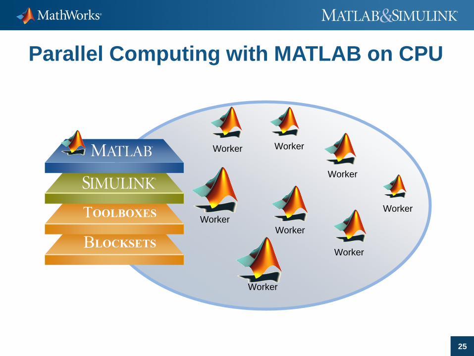
Parallel Computing with MATLAB
Narfi Stefansson
Parallel Computing Development Manager
MathWorks
2
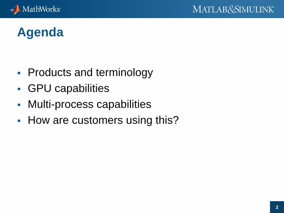
Agenda
Products and terminology
GPU capabilities
Multi-process capabilities
How are customers using this?

3
User’s Desktop
Parallel ComputingToolbox
Compute Cluster
MATLAB DistributedComputing Server
MATLAB Workers
Parallel Computing with MATLAB on CPU
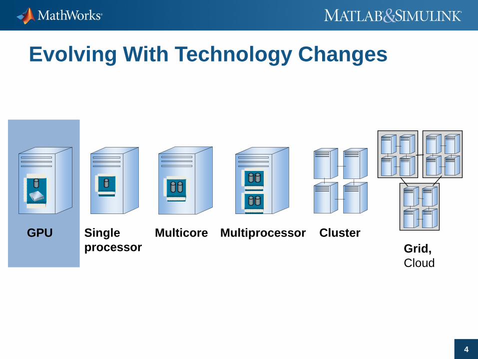
4
Single
processor
Multicore Multiprocessor Cluster
Grid,
Cloud
GPU
Evolving With Technology Changes

5
Why GPUs and why now?
Double support
– Single/double performance inline with expectations
Operations are IEEE Compliant
Cross-platform support now available
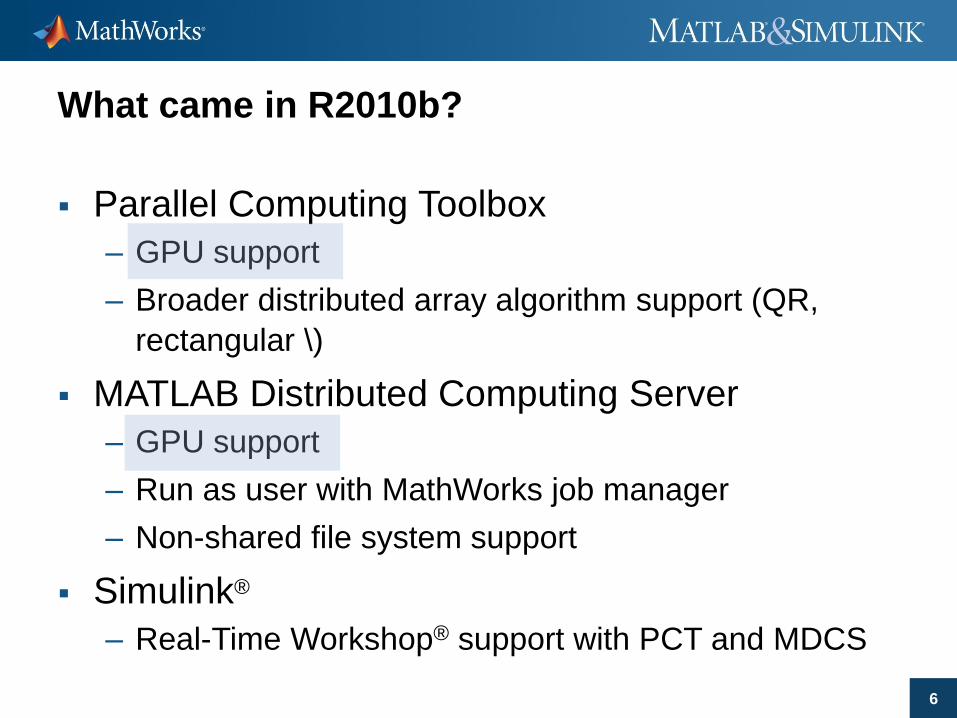
6
What came in R2010b?
Parallel Computing Toolbox
– GPU support
– Broader distributed array algorithm support (QR,
rectangular \)
MATLAB Distributed Computing Server
– GPU support
– Run as user with MathWorks job manager
– Non-shared file system support
Simulink®
– Real-Time Workshop® support with PCT and MDCS

7
What came in R2011a?
Parallel Computing Toolbox
– Deployment of local workers
– More GPU support
– More distributed array algorithm support
MATLAB Distributed Computing Server
– Enhanced support for Microsoft HPC Server
– More GPU support
– Remote service start in Admin Center

8
GPU Support
Call GPU(s) from MATLAB or toolbox/server
worker
Support for CUDA 1.3 enabled devices and up
9
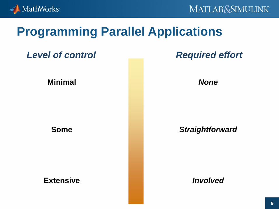
Programming Parallel Applications
Level of control
Minimal
Some
Extensive
Required effort
None
Straightforward
Involved

10
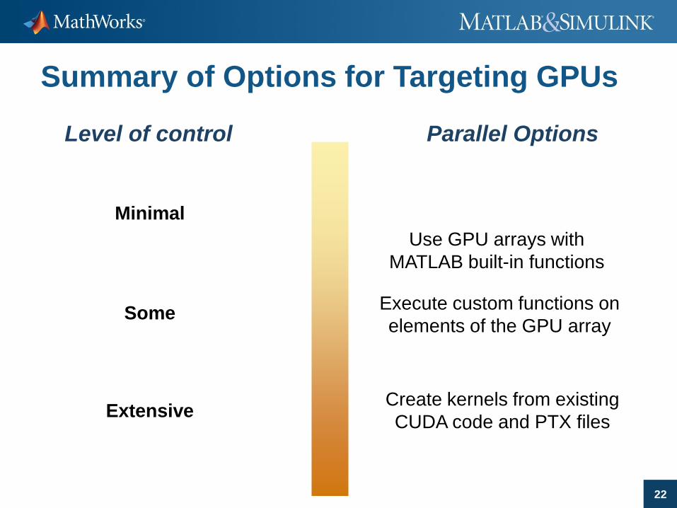
Summary of Options for Targeting GPUs
Level of control
Minimal
Some
Extensive
Parallel Options
Use GPU arrays with
MATLAB built-in functions
Execute custom functions on
elements of the GPU array
Create kernels from existing
CUDA code and PTX files

11
GPU Array Functionality
Array data stored in GPU device memory
Algorithm support for over 100 functions
Integer, single, double, real and complex
support

12
Example:
GPU Arrays
>> A = someArray(1000, 1000);
>> G = gpuArray(A); % Push to GPU memory
…
>> F = fft(G);
>> x = G\b;
…
>> z = gather(x); % Bring back into MATLAB

13
GPUArray Function Support
>100 functions supported
– fft, fft2, ifft, ifft2
– Matrix multiplication (A*B)
– Matrix left division (A\b)
– LU factorization
– ‘ .’
– abs, acos, …, minus, …, plus, …, sin, …
– conv, conv2, filter
– indexing

14
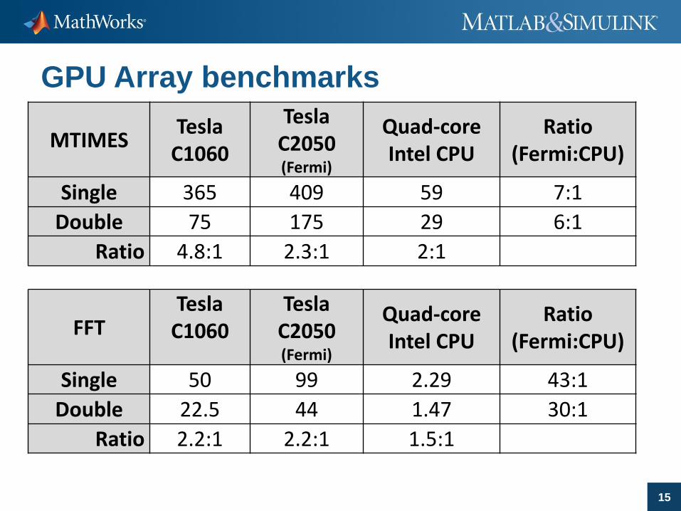
GPU Array benchmarks
* Results in Gflops, matrix size 8192x8192. Limited by card memory.
Computational capabilities not saturated.
A\b*Tesla
C1060
TeslaC2050 (Fermi)
Quad-core Intel CPU
Ratio (Fermi:CPU)
Single 191 250 48 5:1
Double 63.1 128 25 5:1
Ratio 3:1 2:1 2:1
15
GPU Array benchmarks
MTIMESTesla
C1060
TeslaC2050 (Fermi)
Quad-core Intel CPU
Ratio (Fermi:CPU)
Single 365 409 59 7:1
Double 75 175 29 6:1
Ratio 4.8:1 2.3:1 2:1
FFTTesla
C1060Tesla
C2050 (Fermi)
Quad-core Intel CPU
Ratio (Fermi:CPU)
Single 50 99 2.29 43:1
Double 22.5 44 1.47 30:1
Ratio 2.2:1 2.2:1 1.5:1

16
Example:
arrayfun: Element-Wise Operations
>> y = arrayfun(@foo, x); % Execute on GPU
function y = foo(x)
y = 1 + x.*(1 + x.*(1 + x.*(1 + ...
x.*(1 + x.*(1 + x.*(1 + x.*(1 + ...
x.*(1 + x./9)./8)./7)./6)./5)./4)./3)./2);

17
Some arrayfun benchmarks
CPU[4] = multhithreading enabled
CPU[1] = multhithreading disabled
Note: Due to memory constraints, a
different approach is used at N=15 and
above.
18
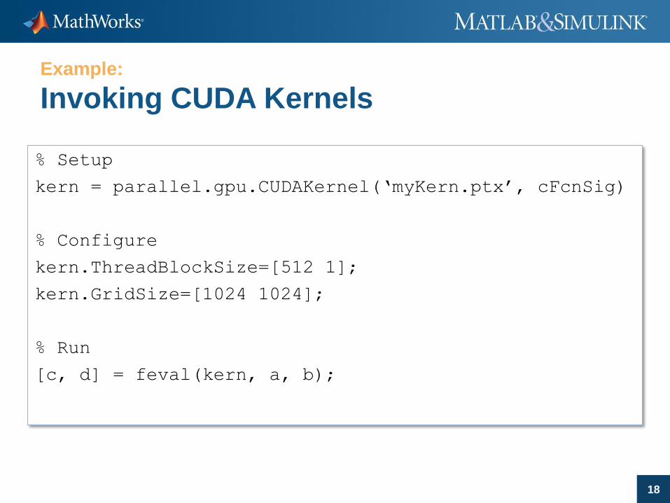
Example:
Invoking CUDA Kernels
% Setup
kern = parallel.gpu.CUDAKernel(‘myKern.ptx’, cFcnSig)
% Configure
kern.ThreadBlockSize=[512 1];
kern.GridSize=[1024 1024];
% Run
[c, d] = feval(kern, a, b);

19
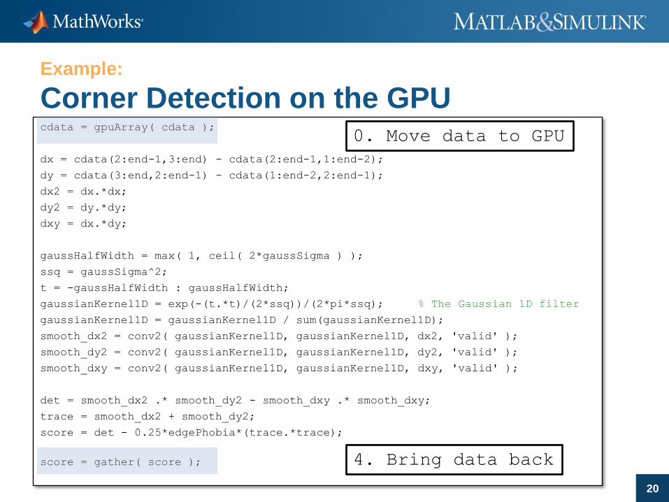
Example:
Corner Detection on the CPU
dx = cdata(2:end-1,3:end) - cdata(2:end-1,1:end-2);
dy = cdata(3:end,2:end-1) - cdata(1:end-2,2:end-1);
dx2 = dx.*dx;
dy2 = dy.*dy;
dxy = dx.*dy;
gaussHalfWidth = max( 1, ceil( 2*gaussSigma ) );
ssq = gaussSigma^2;
t = -gaussHalfWidth : gaussHalfWidth;
gaussianKernel1D = exp(-(t.*t)/(2*ssq))/(2*pi*ssq); % The Gaussian 1D filter
gaussianKernel1D = gaussianKernel1D / sum(gaussianKernel1D);
smooth_dx2 = conv2( gaussianKernel1D, gaussianKernel1D, dx2, 'valid' );
smooth_dy2 = conv2( gaussianKernel1D, gaussianKernel1D, dy2, 'valid' );
smooth_dxy = conv2( gaussianKernel1D, gaussianKernel1D, dxy, 'valid' );
det = smooth_dx2 .* smooth_dy2 - smooth_dxy .* smooth_dxy;
trace = smooth_dx2 + smooth_dy2;
score = det - 0.25*edgePhobia*(trace.*trace);
1. Calculate derivatives
2. Smooth using convolution
3. Calculate score
20
Example:
Corner Detection on the GPUcdata = gpuArray( cdata );
dx = cdata(2:end-1,3:end) - cdata(2:end-1,1:end-2);
dy = cdata(3:end,2:end-1) - cdata(1:end-2,2:end-1);
dx2 = dx.*dx;
dy2 = dy.*dy;
dxy = dx.*dy;
gaussHalfWidth = max( 1, ceil( 2*gaussSigma ) );
ssq = gaussSigma^2;
t = -gaussHalfWidth : gaussHalfWidth;
gaussianKernel1D = exp(-(t.*t)/(2*ssq))/(2*pi*ssq); % The Gaussian 1D filter
gaussianKernel1D = gaussianKernel1D / sum(gaussianKernel1D);
smooth_dx2 = conv2( gaussianKernel1D, gaussianKernel1D, dx2, 'valid' );
smooth_dy2 = conv2( gaussianKernel1D, gaussianKernel1D, dy2, 'valid' );
smooth_dxy = conv2( gaussianKernel1D, gaussianKernel1D, dxy, 'valid' );
det = smooth_dx2 .* smooth_dy2 - smooth_dxy .* smooth_dxy;
trace = smooth_dx2 + smooth_dy2;
score = det - 0.25*edgePhobia*(trace.*trace);
score = gather( score );
0. Move data to GPU
4. Bring data back

21
arrayfun
Can execute entire scalar programs on the GPU
(while, if, for, break, &, &&, …)
function [logCount,t] = mandelbrotElem( x0, y0, r2, maxIter)
% Evaluate the Mandelbrot function for a single element
z0 = complex( x0, y0 );
z = z0;
count = 0;
while count <= maxIter && (z*conj(z) <= r2)
z = z*z + z0;
count = count + 1;
end
% . . . Etc. . . .
22
Summary of Options for Targeting GPUs
Level of control
Minimal
Some
Extensive
Parallel Options
Use GPU arrays with
MATLAB built-in functions
Execute custom functions on
elements of the GPU array
Create kernels from existing
CUDA code and PTX files

23
Parallel Computing enables you to …
Larger Compute Pool Larger Memory Pool
11 26 41
12 27 42
13 28 43
14 29 44
15 30 45
16 31 46
17 32 47
17 33 48
19 34 49
20 35 50
21 36 51
22 37 52
Speed up Computations Work with Large Data

24
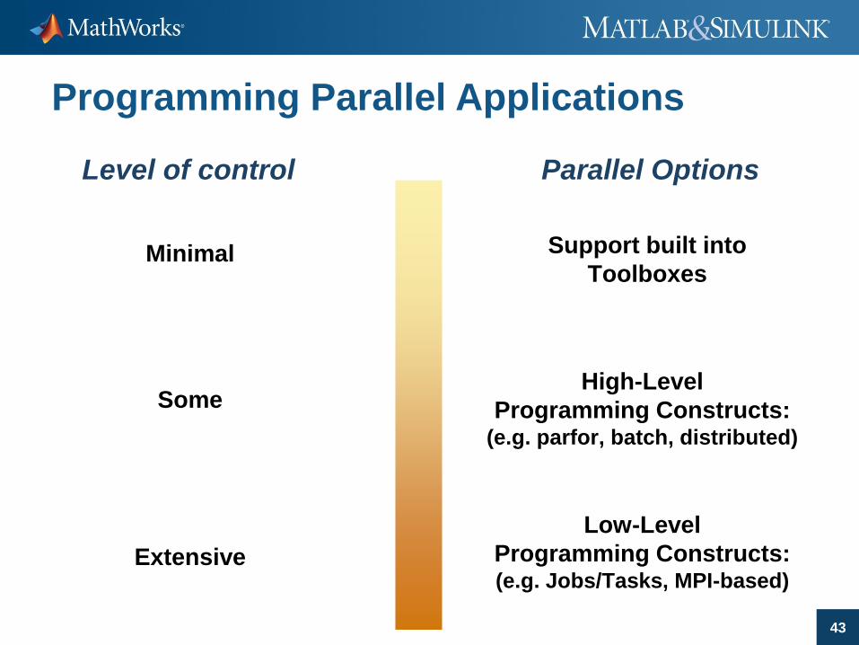
Programming Parallel Applications
Level of control
Minimal
Some
Extensive
Parallel Options
Low-Level
Programming Constructs:(e.g. Jobs/Tasks, MPI-based)
High-Level
Programming Constructs:(e.g. parfor, batch, distributed)
Support built into
Toolboxes
25
Worker Worker
Worker
Worker
WorkerWorker
Worker
WorkerTOOLBOXES
BLOCKSETS
Parallel Computing with MATLAB on CPU
26
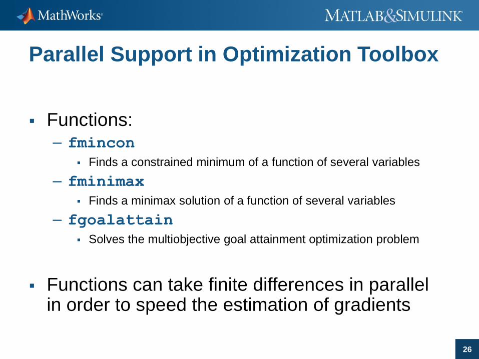
Parallel Support in Optimization Toolbox
Functions: – fmincon
Finds a constrained minimum of a function of several variables
– fminimax
Finds a minimax solution of a function of several variables
– fgoalattain
Solves the multiobjective goal attainment optimization problem
Functions can take finite differences in parallelin order to speed the estimation of gradients

27
Tools with Built-in Support
Optimization Toolbox
Global Optimization Toolbox
Statistics Toolbox
SystemTest
Simulink Design Optimization
Bioinformatics Toolbox
Model-Based Calibration Toolbox
…http://www.mathworks.com/products/parallel-computing/builtin-parallel-support.html
Worker
Worker
Worker
WorkerWorker
Worker
WorkerTOOLBOXES
BLOCKSETS
Directly leverage functions in Parallel Computing Toolbox

28
Programming Parallel Applications
Level of control
Minimal
Some
Extensive
Parallel Options
Low-Level
Programming Constructs:(e.g. Jobs/Tasks, MPI-based)
High-Level
Programming Constructs:(e.g. parfor, batch, distributed)
Support built into
Toolboxes

29
Running Independent Tasks or Iterations
Ideal problem for parallel computing
No dependencies or communications between tasks
Examples include parameter sweeps and Monte Carlo
simulations
Time Time

30
Example: Parameter Sweep of ODEs
Solve a 2nd order ODE
Simulate with differentvalues for b and k
Record peak value for each run
Plot results
0,...2,1,...2,1
5
xkxbxm
0 5 10 15 20 25-0.4
-0.2
0
0.2
0.4
0.6
0.8
1
1.2
Time (s)
Dis
pla
cem
ent
(x)
m = 5, b = 2, k = 2
m = 5, b = 5, k = 5
0
2
4
6 12
34
5
0.5
1
1.5
2
2.5
Stiffness (k)Damping (b)
Pe
ak D
isp
lace
me
nt (x
)

31
Summary of Example
Mixed task-parallel and serial
code in the same function
Ran loops on a pool of
MATLAB resources0 5 10 15 20 25
-0.4
-0.2
0
0.2
0.4
0.6
0.8
1
1.2
Time (s)
Dis
pla
cem
ent
(x)
m = 5, b = 2, k = 2
m = 5, b = 5, k = 5
0
2
4
6 12
34
5
0.5
1
1.5
2
2.5
Stiffness (k)Damping (b)
Pe
ak D
isp
lace
me
nt (x
)

32
The Mechanics of parfor Loops
Pool of MATLAB Workers
a = zeros(10, 1)
parfor i = 1:10
a(i) = i;
end
aa(i) = i;
a(i) = i;
a(i) = i;
a(i) = i;
Worker
Worker
WorkerWorker
1 2 3 4 5 6 7 8 9 101 2 3 4 5 6 7 8 9 10

33
Parallel Computing enables you to …
Larger Compute Pool Larger Memory Pool
11 26 41
12 27 42
13 28 43
14 29 44
15 30 45
16 31 46
17 32 47
17 33 48
19 34 49
20 35 50
21 36 51
22 37 52
Speed up Computations Work with Large Data

34
TOOLBOXES
BLOCKSETS
Distributed Array
Lives on the Cluster
Remotely Manipulate Array
from Desktop
11 26 41
12 27 42
13 28 43
14 29 44
15 30 45
16 31 46
17 32 47
17 33 48
19 34 49
20 35 50
21 36 51
22 37 52
Client-side Distributed Arrays

35
Enhanced MATLAB Functions That
Operate on Distributed Arrays

36
Programming Parallel Applications
Level of control
Minimal
Some
Extensive
Parallel Options
Low-Level
Programming Constructs:(e.g. Jobs/Tasks, MPI-based)
High-Level
Programming Constructs:(e.g. parfor, batch, distributed)
Support built into
Toolboxes

37
spmd blocks
spmd
% single program across workers
end
Mix parallel and serial code in the same function
Run on a pool of MATLAB resources
Single Program runs simultaneously across workers
– Distributed arrays, message-passing
Multiple Data spread across multiple workers
– Data stays on workers

39
Client-side Distributed Arrays and SPMD
Client-side distributed arrays– Class distributed
– Can be created and manipulated directly from the client.
– Simpler access to memory on labs
– Client-side visualization capabilities
spmd
– Block of code executed on workers
– Worker specific commands
– Explicit communication between workers
– Mixture of parallel and serial code

40
MPI-Based Functions in
Parallel Computing Toolbox™
Use when a high degree of control over parallel algorithm is required
High-level abstractions of MPI functions
– labSendReceive, labBroadcast, and others
– Send, receive, and broadcast any data type in MATLAB
Automatic bookkeeping
– Setup: communication, ranks, etc.
– Error detection: deadlocks and miscommunications
Pluggable
– Use any MPI implementation that is binary-compatible with MPICH2

41
Scheduling Jobs and Tasks
TOOLBOXES
BLOCKSETS
Scheduler
Job
Results
Worker
Worker
Worker
Worker
Task
Result
Task
Task
Task
Result
Result
Result

42
Open API for others
Support for Schedulers
Direct Support
TORQUE
43
Programming Parallel Applications
Level of control
Minimal
Some
Extensive
Parallel Options
Low-Level
Programming Constructs:(e.g. Jobs/Tasks, MPI-based)
High-Level
Programming Constructs:(e.g. parfor, batch, distributed)
Support built into
Toolboxes

44
Research Engineers Advance Design
of the International Linear Collider with
MathWorks Tools
ChallengeDesign a control system for ensuring the precise
alignment of particle beams in the International Linear
Collider
SolutionUse MATLAB, Simulink, Parallel Computing Toolbox,
and Instrument Control Toolbox software to design,
model, and simulate the accelerator and alignment
control system
Results Simulation time reduced by an order of magnitude
Development integrated
Existing work leveraged
“Using Parallel Computing Toolbox,
we simply deployed our simulation
on a large group cluster. We saw a
linear improvement in speed, and we
could run 100 simulations at once.
MathWorks tools have enabled us to
accomplish work that was once
impossible.”
Dr. Glen White
Queen Mary, University of London
Queen Mary high-throughput cluster.
Link to user story

45
Edwards Air Force Base Accelerates Flight
Test Data Analysis Using MATLAB and
MathWorks Parallel Computing Tools
ChallengeAccelerate performance and flying qualities flight test
data analysis for unmanned reconnaissance aircraft
Solution
Use MathWorks parallel computing tools to execute
MATLAB flight data processing algorithms on a
16-node computer cluster
Results Analysis completed 16 times faster
Application parallelized in minutes
Program setup time reduced from weeks to days
Parallel Computing Toolbox and
MATLAB Distributed Computing
Server provided a one-for-one time
savings with the number of
processors used. For example,
with a 16-processor cluster,
throughput was 16 times higher,
enabling Edwards AFB engineers
to accomplish in hours tasks that
used to take days.
Link to user story
A Global Hawk test flight.

46
Argonne National Laboratory Develops
Powertrain Systems Analysis Toolkit with
MathWorks Tools
Challenge
Evaluate designs and technologies for hybrid and fuel cell
vehicles
Solution
Use MathWorks tools to model advanced vehicle
powertrains and accelerate the simulation of hundreds
of vehicle configurations
Results Distributed simulation environment developed in
one hour
Simulation time reduced from two weeks to
one day
Simulation results validated using vehicle test data
“We developed an advanced
framework and scalable powertrain
components in Simulink, designed
controllers with Stateflow,
automated the assembly of models
with MATLAB scripts, and then
distributed the complex simulation
runs on a computing cluster – all
within a single environment."
Sylvain Pagerit
Argonne National Laboratory
Vehicle model created with PSAT.
Link to user story