GPU-Accelerated Preconditioned Iterative Linear Solvers∗

Ruipeng Li † Yousef Saad†

Abstract

This work is an overview of our preliminary experience in developing high-performance it-erative linear solver accelerated by GPU co-processors. Our goal is to illustrate the advantagesand difficulties encountered when deploying GPU technology to perform sparse linear algebracomputations. Techniques for speeding up sparse matrix-vector product (SpMV) kernels andfinding suitable preconditioning methods are discussed. Our experiments with an NVIDIATESLA C1060 show that for unstructured matrices SpMV kernels can be up to 10 times fasteron the GPU than on the host Intel Xeon E5504 Processor. Overall performance of the GPU-accelerated Incomplete Cholesky (IC) factorization preconditioned CG method can outperformits CPU counterpart by a much smaller factor, up to 3, and GPU-accelerated Incomplete LU(ILU) factorization preconditioned GMRES method can achieve a speedup nearing 4. However,with better suited preconditioning techniques for GPUs, this performance can be significantlyimproved.

1 Introduction

Emerging many-core platforms yield enormous raw processing power, in the form of massive SIMDparallelism. Chip designers are increasing processing capabilities by building multiple processingcores in a single chip. The number of cores that can fit into a chip is increasing at a fast pace and as aresult Moore’s Law has been given a new interpretation: it is the number of cores that doubles every18 months [1]. The NVIDIA GPU (Graphics Processing Unit) is one of several available coprocessorsthat feature a large number of cores. Traditionally, GPUs have been especially designed to handlecomputations for computer graphics in real-time. Today, they are increasingly being exploitedas general-purpose attached processors to speed-up computations in image processing, physicalsimulations, data mining, linear algebra, etc.

CUDA (Compute Unified Device Architecture) is a parallel language for NVIDIA GPUs, whichsupports developers to programming on GPU in C/C++ with NVIDIA extensions. Wrappers forPython, Fortran, Java and MATLAB are also available. This paper explores various aspects ofsparse linear algebra computations on GPUs. Specifically, we investigate appropriate precondition-ing methods for high-performance iterative linear solvers accelerated by GPUs.

The remainder of this report is organized as follows: Section 2 gives a brief introduction of GPUarchitectures, the CUDA programming model, and related work. Section 3 describes the sparsematrix-vector product (SpMV) kernel on GPUs; Section 4 describes sparse triangular solves andthe preconditioned iterative methods, CG and GMRES are discussed in Section 5; Section 6 reportson experimental results and analyses. Finally, concluding remarks are stated in Section 7.

∗This work is supported by DOE under grant DE-FG 08ER 25841 and by the Minnesota Supercomputer Institute.†Department of Computer Science & Engineering; University of Minnesota; Department of Computer Science &

Engineering; Minneapolis, MN 55455, USA.

1

2 GPU Architecture and CUDA

2.1 GPU Architecture

A GPU is built as a scalable array of multi-threaded Streaming Multiprocessors (SMs), each ofwhich consists of multiple Scalar Processor (SP) cores. To manage hundreds of threads, the multi-processors employs a Single Instruction Multiple Threads (SIMT) model. Each thread is mappedinto one SP core and executes independently with its own instruction address and register state[18].

The NVIDIA GPU platform has various memory hierarchies. The types of memory can beclassified as follows: (1) off-chip global memory, (2) off-chip local memory, (3) on-chip sharedmemory, (4) read-only cached off-chip constant memory and texture memory and (5) registers. Theeffective bandwidth of each type of memory depends significantly on the access pattern. Globalmemory is relatively large but has a much higher latency (from 400 to 800 cycles for the NVIDIAGPUs) compared with the on-chip shared memory (1 clock cycle if there are no bank conflicts).Global memory is not cached, so it is important to follow the right access pattern to achieve goodmemory bandwidth.

Threads are organized in warps. A warp is defined as a group of 32 threads of consecutive threadIDs. A half-warp is either the first or second half of a warp. The most efficient way to use the global

memory bandwidth is to coalesce the simultaneous memory accesses by threads in a half-warp intoa single memory transaction. For NVIDIA GPU devices with ’compute capability’ 1.2 and higher,memory access by a half-warp is coalesced as soon as the words accessed by all threads lie in thesame segment of size equal to 128 bytes if all threads access 32-bit or 64-bit words. Local memoryaccesses are always coalesced. Alignment and coalescing techniques are explained in details in [18].Since it is on chip, the shared memory is much faster than the global memory but we also need topay attention to the problems of bank conflict. The size of shared memory is 16K per SM. Cachedconstant memory and texture memory are also beneficial for accessing reused data and data with2D spatial locality.

2.2 CUDA Programming

Programming NVIDIA GPUs for general-purpose computing is supported by the NVIDIA CUDA(Compute Unified Device Architecture) environment. CUDA programs on the host (CPU) invoke akernel grid which runs on the device (GPU). The same parallel kernel is executed by many threads.These threads are organized into thread blocks. Thread blocks are distributed to SMs and splitinto warps scheduled by SIMT units. All threads in the same thread block share the same sharedmemory of size 16 KB and can synchronize themselves by a barrier. Threads in a warp execute onecommon instruction at a time. This is referred to as warp-level synchronization [18]. Full efficiencyis achieved when all 32 threads of a warp follow the same execution path. Branch divergence causesserial execution.

2.3 Related Work

The potential of GPUs for parallel sparse matrix computations was recognized early on when GPUprogramming required shader languages [6]. After the advent of NVIDIA CUDA, GPUs have drawnmuch more attention for sparse linear algebra and the solution of sparse linear systems. Existingimplementations of the GPU Sparse matrix-vector product (SpMV) include CUDPP (CUDA DataParallel Primitives) library [24], NVIDIA CUSPARSE library [5] and the IBM SpMV library [4].

2

In [4, 5], different formats of sparse matrices are studied for producing high performance SpMVkernels on GPUs.

A GPU-accelerated Jacobi preconditioned CG method is studied in [12]. In [3], the CG methodwith incomplete Poisson preconditioning is proposed for the Poisson problem on a multi-GPU plat-form. The Block-ILU preconditioned GMRES method is studied for solving sparse linear systemson the NVIDIA Tesla GPUs in [27]. SpMV kernels on GPUs and the Block-ILU preconditionedGMRES method are used in [16, 25] for solving large sparse linear systems in black-oil and com-positional flow simulations. A GPU implementation of deflated PCG method for bubbly flowcomputations is discussed in [13].

For dense linear algebra computations, the Matrix Algebra for GPU and Multicore Architectures(MAGMA) project [2] using hybrid multicore-multiGPU system aims to develop a dense linearalgebra library similar to LAPACK. They reported speeds up to 375/75 GFLOPS in single/doubleprecision for the GEMM matrix-matrix operation, and 280 GFLOPS in single precision for solving alinear system by the L/U factorization using multiple GPUs. Vasily Volkov and James Demmel[26] reported that they were able to approach the peak performance of the G80 series GPUs fordense matrix-matrix multiplications.

3 Sparse Matrix-Vector Product

The sparse matrix-vector product (SpMV) is one of the major components of any sparse matrixcomputations. However, the SpMV kernel which accounts for a big part of the cost of sparseiterative linear solvers, has difficulty in reaching a significant percentage of peak floating pointthroughput. It yields only a small fraction of the machine peak performance due to its indirectand irregular memory accesses [4]. Recently, several research groups have reported their imple-mentations on high-performance sparse matrix-vector multiplication kernels on GPUs [10, 5, 4].NVIDIA researchers have demonstrated that their SpMV kernels can reach 15 GFLOPS and 10GFLOPS in single/double precision for unstructured mesh matrices [5]. This section, will discussimplementation of SpMV GPU kernels using several different formats.

For a matrix-vector product, y = Ax, data reuse can be applied to the vector x which is read-only. Therefore, a good strategy is to place the vector x in the cached texture memory and accessit by texture fetching [18]. As reported in [5], caching improves the throughput by an average of30% and 25% in single and double precision respectively.

3.1 SpMV in CSR Format

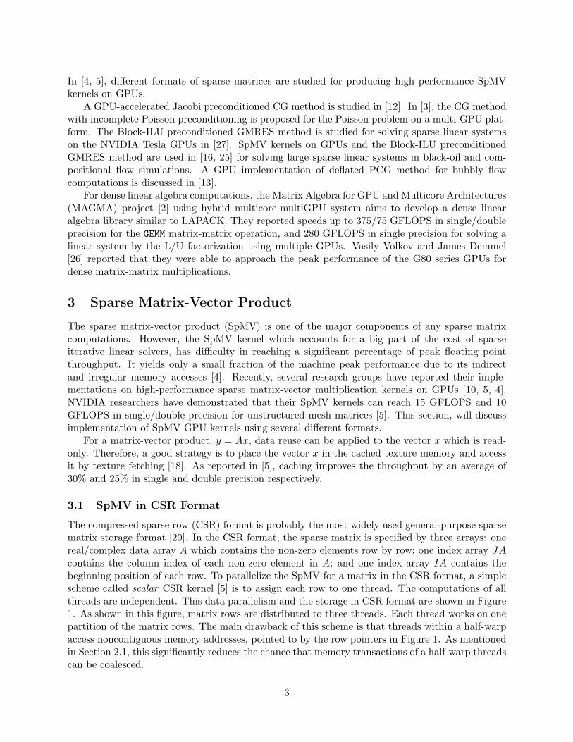
The compressed sparse row (CSR) format is probably the most widely used general-purpose sparsematrix storage format [20]. In the CSR format, the sparse matrix is specified by three arrays: onereal/complex data array A which contains the non-zero elements row by row; one index array JAcontains the column index of each non-zero element in A; and one index array IA contains thebeginning position of each row. To parallelize the SpMV for a matrix in the CSR format, a simplescheme called scalar CSR kernel [5] is to assign each row to one thread. The computations of allthreads are independent. This data parallelism and the storage in CSR format are shown in Figure1. As shown in this figure, matrix rows are distributed to three threads. Each thread works on onepartition of the matrix rows. The main drawback of this scheme is that threads within a half-warpaccess noncontiguous memory addresses, pointed to by the row pointers in Figure 1. As mentionedin Section 2.1, this significantly reduces the chance that memory transactions of a half-warp threadscan be coalesced.

3

...

...

Data

Col Indices

Row pointers ...

Thread2 Thread3 Thread1 Thread2 ...Thread1Row1 Row2 Row3 Row4 Row5

Figure 1: Scalar CSR SpMV Kernel

A better approach, termed vector CSR kernel, is to assign a half-warp (16 threads) instead ofonly one thread to each row. In this approach, the first half-warp works on row one, the secondworks on row two, and so on. Since all threads within a half-warp access non-zero elements ofsome row, these accesses are more likely to belong to the same memory segment. So the chanceof coalescing should be higher. But this approach incurs another problem related to computingvector dot products in parallel (dot product of a matrix row vector with the vector x). To solvethis problem, each thread saves its partial result into the shared memory and a parallel reduction isused to sum up all partial results [4, 5]. Moreover, since a warp executes one common instructionat a time, threads within a warp are implicitly synchronized and so the synchronization in thehalf-warp parallel reduction can be omitted for better performance [18]. In addition, full efficiencyof the vector CSR kernel requires at least 16 non-zeros per row in A. Our vector CSR kernel isslightly different from the implementation in [5] in which a warp of threads are assigned to eachrow.

3.2 SpMV in JAD Format

The JAD (JAgged Diagonal) format can be viewed as a generalization of the Ellpack-Itpack formatwhich removes the assumption on the fixed-length rows [22]. To build the JAD structure, we firstsort the rows by non-increasing order of the number of non-zeros per row. Then the first JADconsists of the first element of each row; the second JAD consists of the second element, etc. Thenumber of JADs is the largest number of non-zeros per row. An example is shown below.

A =

1 0 2 0 03 4 0 5 00 6 7 0 80 0 9 10 00 0 0 11 12

, PA =

3 4 0 5 00 6 7 0 81 0 2 0 00 0 9 10 00 0 0 11 12

Here, A is the original matrix and PA is the reordered matrix. Then the JAD format of Ais shown in Table 1. The JAD data structure also consist of three arrays: one real/complex dataarray DJ contains the non-zero elements; one index array JDIAG contains the column index of eachnon-zero; and one index array IDIAG contains the beginning position of each JAD.

Like in the scalar CSR kernel, only one thread works on each matrix row to exploit fine-grainedparallelism. Note that since matrix data and indices are stored in the JAD format, the JAD kerneldoes not suffer from the performance drawback of the scalar CSR kernel: consecutive threads canaccess contiguous memory addresses, which follows the suggested memory access pattern and canimprove the memory bandwidth by coalescing memory transactions. This memory access pattern

4

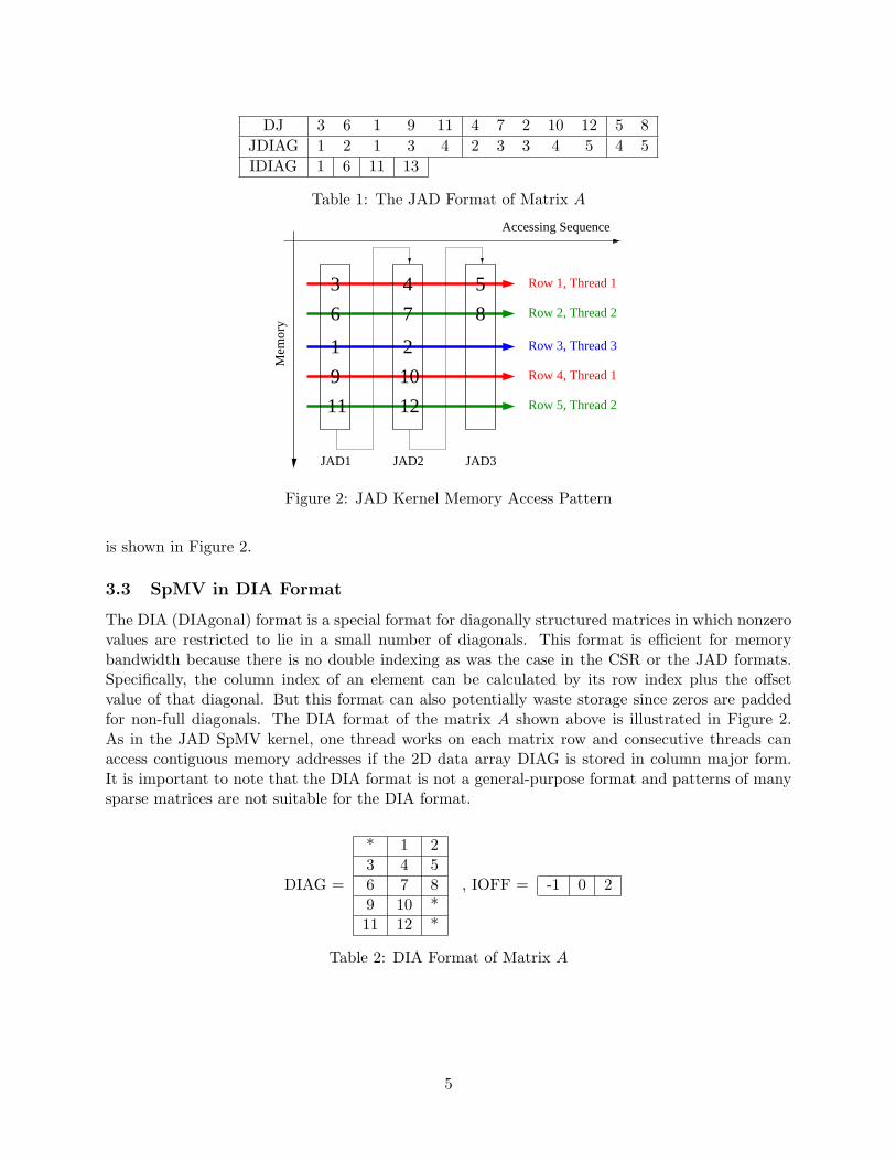
DJ 3 6 1 9 11 4 7 2 10 12 5 8

JDIAG 1 2 1 3 4 2 3 3 4 5 4 5

IDIAG 1 6 11 13

Table 1: The JAD Format of Matrix A

3

6

1

9

11

8

4

7

2

12

10

5 Row 1, Thread 1

Row 2, Thread 2

Row 3, Thread 3

Row 4, Thread 1

Row 5, Thread 2

Mem

ory

Accessing Sequence

JAD1 JAD3JAD2

Figure 2: JAD Kernel Memory Access Pattern

is shown in Figure 2.

3.3 SpMV in DIA Format

The DIA (DIAgonal) format is a special format for diagonally structured matrices in which nonzerovalues are restricted to lie in a small number of diagonals. This format is efficient for memorybandwidth because there is no double indexing as was the case in the CSR or the JAD formats.Specifically, the column index of an element can be calculated by its row index plus the offsetvalue of that diagonal. But this format can also potentially waste storage since zeros are paddedfor non-full diagonals. The DIA format of the matrix A shown above is illustrated in Figure 2.As in the JAD SpMV kernel, one thread works on each matrix row and consecutive threads canaccess contiguous memory addresses if the 2D data array DIAG is stored in column major form.It is important to note that the DIA format is not a general-purpose format and patterns of manysparse matrices are not suitable for the DIA format.

* 1 23 4 5

DIAG = 6 7 89 10 *11 12 *

, IOFF = -1 0 2

Table 2: DIA Format of Matrix A

5

4 Sparse Triangular Solve

In the row version of the standard forward and backward substitution algorithms for solving trian-gular systems, the outer loop of the substitution for each unknown is sequential. The inner loop isa vector dot product of a sparse row vector of the triangular matrix and the dense right-hand-sidevector b. In the column oriented versions, the inner loop is a saxpy operation of a sparse columnvector and the vector b. These dot product and saxpy operations can be split and parallelized butthis approach is not efficient in general since the length of the vector involved is usually short.

4.1 Level Scheduling

Better parallelism can be achieved by level scheduling, which exploits topological sorting [22]. Theidea is to group unknowns x(i) into different levels so that all unknowns within the same level canbe computed simultaneously. For forward substitution, the level of unknown x(i), denoted by l(i)can be computed as follow after initializing l(j) = 0 for all j,

l (i) = 1 + maxj{l (j)}, for all j such that Lij 6= 0 .

If nlev is the number of levels, the permutation array q records the ordering of all unknowns, levelby level and level (i) points to the beginning of the ith level in array q, then forward substitutionwith level scheduling is shown in Algorithm 1. The inequality, 1 ≤ nlev ≤ n is satisfied, wheren is the size of the system. The best case when nlev = 1, corresponds to the situation when allunknowns can be computed simultaneously (e.g., L is a diagonal matrix). In the worst case, whennlev = n, the forward substitution is completely sequential. The analogous back substitution ishandled similarly.

Algorithm 1 Forward Substitution with Level Scheduling

1: for lev = 1 : nlev do

2: j1 = level (lev)3: j2 = level (lev + 1)− 14: for k = j1 : j2 do

5: i = q (k)6: for j = ial (i) : ial (i + 1)− 1 do

7: x(i)← x(i)− al(j)× x(jal(j))8: end for

9: end for

10: end for

4.2 GPU Implementation

The implementation of the row version of forward/backward substitution kernel is similar to thevector CSR format SpMV kernel. With level scheduling, the equations are partitioned into levels.Starting from the first level, each half-warp picks one unknown of the current level to solve andthe vector dot product is split and summed up by parallel reduction of the partial results as wasdone in the vector CSR format SpMV kernel. Synchronization among half-warps is needed aftereach level is finished. The performance of parallel triangular solve on GPUs significantly dependson the number of levels of triangular matrices. For some cases, some reordering technique like

6

the Multiple Minimal Degree (MMD) ordering [11], may help reduce the number of levels so as toincrease parallelism. However, the performance of the sparse triangular solve on GPUs is usuallyfar lower than that of sparse matrix-vector products and typically even lower than the sequentialimplementation on CPUs.

5 Preconditioned Iterative Methods

Linear systems are often derived from discretization of partial differential equations by finite dif-ference method, finite element method or finite volume method. Matrices from these applicationsare usually large and sparse, which means that a large number of the entries of A are zeros. TheConjugate Gradient (CG) and the Generalized Minimal RESidual (GMRES) methods, see, e.g.,[22], are extensively used Krylov subspace methods for solving symmetric positive definite (SPD)/non-symmetric linear systems iteratively. These are termed accelerators.

A preconditioner is any form of implicit or explicit modification of an original system that makeit easier to solve by a given accelerator [22]. The right preconditioned linear system takes the form:

AM−1u = b, u = Mx.

The matrix M is the preconditioning matrix. It should be close to A, i.e., M ≈ A and thepreconditioning operation M−1v should be easy to apply for an arbitrary vector v.

The main computational components in the preconditioned CG or GMRES methods are: (1)Matrix-vector product; (2) Preconditioning operation; (3) Level-1 BLAS vector operations. Pre-conditioned iterative methods can be speeded-up by the GPU SpMV kernels and the CUBLASlibrary which is an implementation of BLAS library on top of the NVIDIA CUDA driver [17].

The convergence rate of iterative methods is highly dependent on the quality of the precon-ditioner used. Computational complexities of different types of preconditioning operations aredifferent. Moreover, their performance varies significantly on different computing platforms. In thefollowing sections, several types of preconditioners along with their GPU implementations will bediscussed in detail.

5.1 ILU/IC Preconditioners

The Incomplete LU (ILU) factorization process for a sparse matrix A computes a sparse lowertriangular matrix L and a sparse upper triangular matrix U such that the residual matrix R =LU − A satisfies certain conditions [22]. Since the preconditioning matrix M = LU and LU ≈A, the preconditioning operation is a back substitution followed by a forward substitution, i.e.,u = M−1v = U−1L−1v. If no fill-in is allowed in ILU process, we obtain the so called ILU(0)preconditioner. The zero pattern of L and U is exactly the same as that of A. The accuracy ofthis ILU(0) factorization preconditioning may be not sufficient in many cases. The more accurateILU(k) factorization allows more fill-ins by using the notion of level-fill-in. ILUT approach usesan alternative method to drop fill-ins. Instead of levels, it drops entries based on the numericalvalues of the fill-in elements. If the value is smaller than some threshold, it is zeroed out. Detailsare discussed in [22]. When A is SPD, the incomplete Cholesky (IC) factorization is used as apreconditioner for the CG method. However, the incomplete Cholesky factorization for an SPDmatrix does not always exist. The modified incomplete Cholesky (MIC) factorization discussed in[19] is used, which exists for any SPD matrix.

As mentioned in Section 4.2, the performance of a triangular solve on GPUs deteriorates severelywhen the number of level increases. Triangular systems obtained from ILU or IC factorizations

7

����������������

����������������

�������������������������

�������������������������

�������������������������

�������������������������

��������������������

��������������������

��������������������

��������������������

LU

A1

An

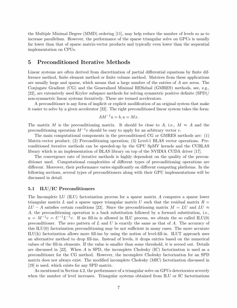
Figure 3: Block Jacobi+ILU Preconditioner

which allow many fill-ins usually have a large number of levels. Although MMD reordering can helpincrease parallelism in some cases, in general, triangular solves on GPUs are still slower than on theCPU due to their sequential nature. Therefore, the triangular solves which are slow on the GPU canbe executed on the CPU for better performance. This implies transferring data (the preconditionedvector) between CPU and GPU in each iteration step. In CUDA, page-locked/mapped host memorycan be used to this portion of data to achieve higher memory bandwidth [18]. Although thisviolates one of the performance guidelines in [18], ’minimize data transfer between the host and

the device...even if that means running kernels with low parallelism computations’, this hybridCPU/GPU computation still exhibits a higher performance than performing the triangular solveson GPUs.

To obtain a higher speed-up from the GPU, parallel preconditioners that are better suitedfor GPU parallelism must be developed and implemented. The Block Jacobi preconditioners,multi-color SSOR/ILU(0) preconditioners and polynomial preconditioners discussed in the followingsections try to achieve high performance in this way.

5.2 Block Jacobi Preconditioners

The simplest parallel preconditioner might be the block Jacobi technique which breaks up thesystem into independent local sub-systems. These subsystems correspond to the diagonal blocks inthe reordered matrix illustrated in Figure 3. The global solution is obtained by adding solutionsof all local systems and these local systems can be solved approximately by ILU factorizations.The setup and application phases of the preconditioner can be performed locally without datadependency. Therefore, one CUDA thread block is assigned to each local block and no globalsynchronization or communication is needed. Threads within each thread block can cooperate tosolve the local system and save the local results to the global output vector.

Although block Jacobi preconditioner with a large number of blocks can provide high parallelism,a well-known drawback is that it usually results in a much larger number of iterations to converge.The benefits of increased parallelism may be outweighed by the increased number of iterations.

5.3 Multi-Color SSOR/ILU(0) Preconditioners

A graph G is p-colorable if its vertices can be colored in p colors such that no two adjacent verticeshave the same color. A simple greedy algorithm known as sequential coloring algorithm can provide

8

an adequate coloring in a number of colors upper bounded by ∆ (G) + 1, where ∆ (G) is themaximum degree of vertices of G.

Suppose a graph is colored by p colors and its vertices are reordered into p blocks by colors.Then its reordered adjacency matrix A has the following structure:

D1

D2 −F. . .

−E Dp−1

Dp

,

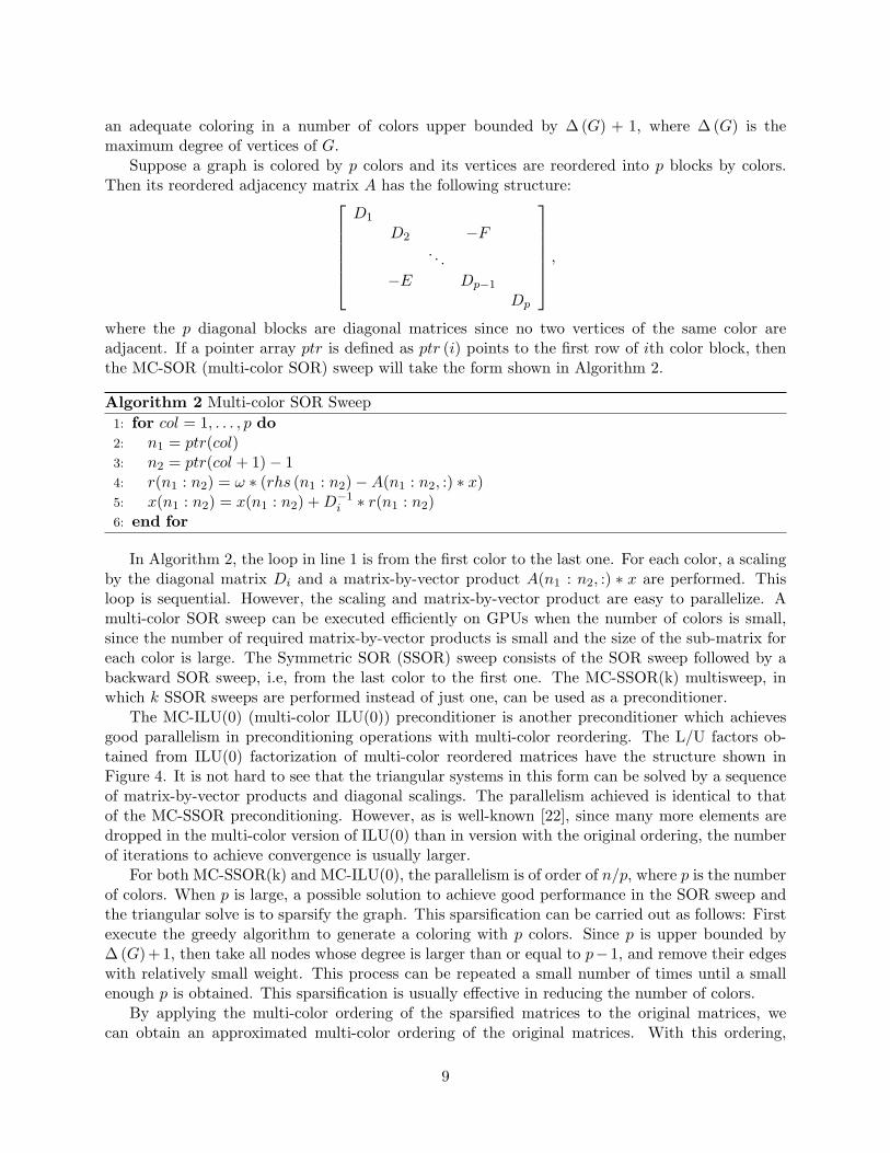
where the p diagonal blocks are diagonal matrices since no two vertices of the same color areadjacent. If a pointer array ptr is defined as ptr (i) points to the first row of ith color block, thenthe MC-SOR (multi-color SOR) sweep will take the form shown in Algorithm 2.

Algorithm 2 Multi-color SOR Sweep

1: for col = 1, . . . , p do

2: n1 = ptr(col)3: n2 = ptr(col + 1)− 14: r(n1 : n2) = ω ∗ (rhs (n1 : n2)−A(n1 : n2, :) ∗ x)5: x(n1 : n2) = x(n1 : n2) + D−1

i ∗ r(n1 : n2)6: end for

In Algorithm 2, the loop in line 1 is from the first color to the last one. For each color, a scalingby the diagonal matrix Di and a matrix-by-vector product A(n1 : n2, :) ∗ x are performed. Thisloop is sequential. However, the scaling and matrix-by-vector product are easy to parallelize. Amulti-color SOR sweep can be executed efficiently on GPUs when the number of colors is small,since the number of required matrix-by-vector products is small and the size of the sub-matrix foreach color is large. The Symmetric SOR (SSOR) sweep consists of the SOR sweep followed by abackward SOR sweep, i.e, from the last color to the first one. The MC-SSOR(k) multisweep, inwhich k SSOR sweeps are performed instead of just one, can be used as a preconditioner.

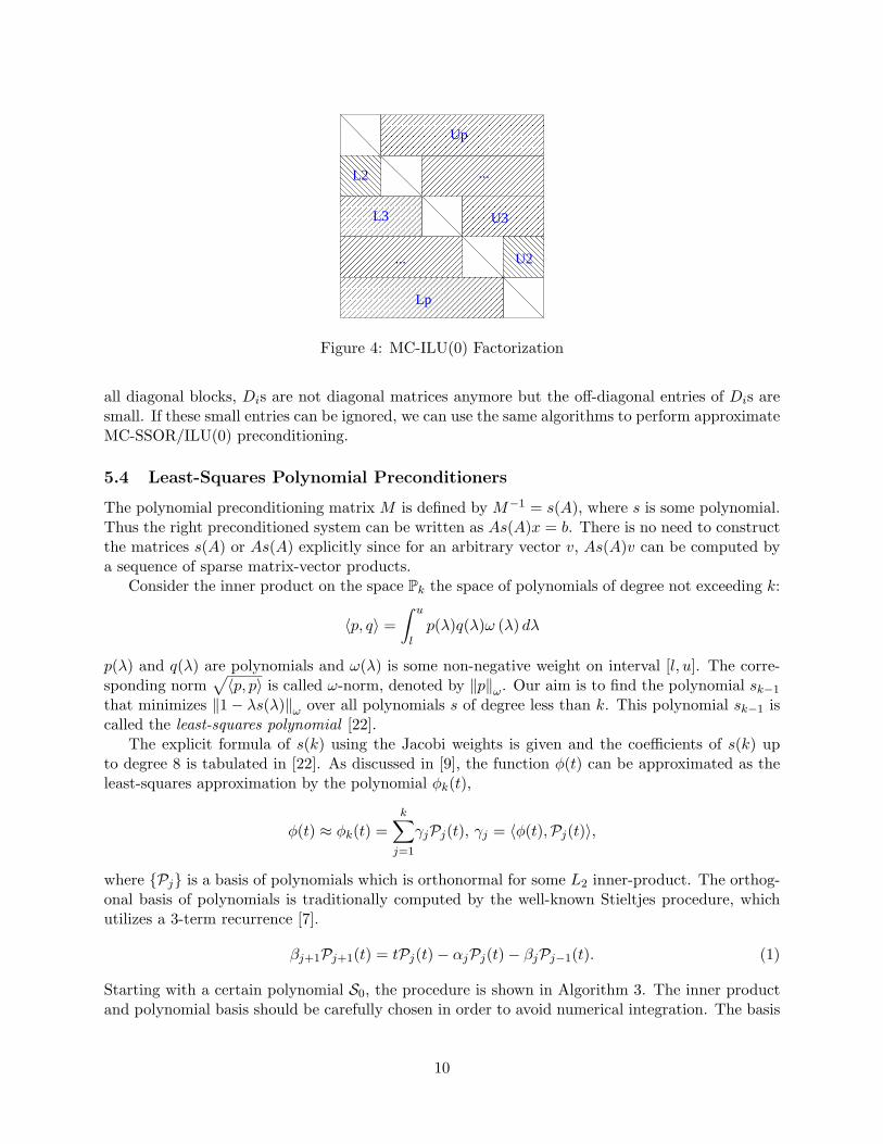
The MC-ILU(0) (multi-color ILU(0)) preconditioner is another preconditioner which achievesgood parallelism in preconditioning operations with multi-color reordering. The L/U factors ob-tained from ILU(0) factorization of multi-color reordered matrices have the structure shown inFigure 4. It is not hard to see that the triangular systems in this form can be solved by a sequenceof matrix-by-vector products and diagonal scalings. The parallelism achieved is identical to thatof the MC-SSOR preconditioning. However, as is well-known [22], since many more elements aredropped in the multi-color version of ILU(0) than in version with the original ordering, the numberof iterations to achieve convergence is usually larger.

For both MC-SSOR(k) and MC-ILU(0), the parallelism is of order of n/p, where p is the numberof colors. When p is large, a possible solution to achieve good performance in the SOR sweep andthe triangular solve is to sparsify the graph. This sparsification can be carried out as follows: Firstexecute the greedy algorithm to generate a coloring with p colors. Since p is upper bounded by∆ (G)+1, then take all nodes whose degree is larger than or equal to p−1, and remove their edgeswith relatively small weight. This process can be repeated a small number of times until a smallenough p is obtained. This sparsification is usually effective in reducing the number of colors.

By applying the multi-color ordering of the sparsified matrices to the original matrices, wecan obtain an approximated multi-color ordering of the original matrices. With this ordering,

9

�������������������������

�������������������������

���������������������������������������������

���������������������������������������������

����������������������������������������

����������������������������������������

�����������������������������������������������������������������

�����������������������������������������������������������������

������������������������������������������������������������

������������������������������������������������������������

��������������������

��������������������

��������������������������������������������������������������������

��������������������������������������������������������������������

��������������������������������������������������������������������������������

��������������������������������������������������������������������������������

L2

L3

...

Lp

...

U2

U3

Up

Figure 4: MC-ILU(0) Factorization

all diagonal blocks, Dis are not diagonal matrices anymore but the off-diagonal entries of Dis aresmall. If these small entries can be ignored, we can use the same algorithms to perform approximateMC-SSOR/ILU(0) preconditioning.

5.4 Least-Squares Polynomial Preconditioners

The polynomial preconditioning matrix M is defined by M−1 = s(A), where s is some polynomial.Thus the right preconditioned system can be written as As(A)x = b. There is no need to constructthe matrices s(A) or As(A) explicitly since for an arbitrary vector v, As(A)v can be computed bya sequence of sparse matrix-vector products.

Consider the inner product on the space Pk the space of polynomials of degree not exceeding k:

〈p, q〉 =

∫ u

l

p(λ)q(λ)ω (λ) dλ

p(λ) and q(λ) are polynomials and ω(λ) is some non-negative weight on interval [l, u]. The corre-sponding norm

√

〈p, p〉 is called ω-norm, denoted by ‖p‖ω. Our aim is to find the polynomial sk−1

that minimizes ‖1− λs(λ)‖ω over all polynomials s of degree less than k. This polynomial sk−1 iscalled the least-squares polynomial [22].

The explicit formula of s(k) using the Jacobi weights is given and the coefficients of s(k) upto degree 8 is tabulated in [22]. As discussed in [9], the function φ(t) can be approximated as theleast-squares approximation by the polynomial φk(t),

φ(t) ≈ φk(t) =k

∑

j=1

γjPj(t), γj = 〈φ(t),Pj(t)〉,

where {Pj} is a basis of polynomials which is orthonormal for some L2 inner-product. The orthog-onal basis of polynomials is traditionally computed by the well-known Stieltjes procedure, whichutilizes a 3-term recurrence [7].

βj+1Pj+1(t) = tPj(t)− αjPj(t)− βjPj−1(t). (1)

Starting with a certain polynomial S0, the procedure is shown in Algorithm 3. The inner productand polynomial basis should be carefully chosen in order to avoid numerical integration. The basis

10

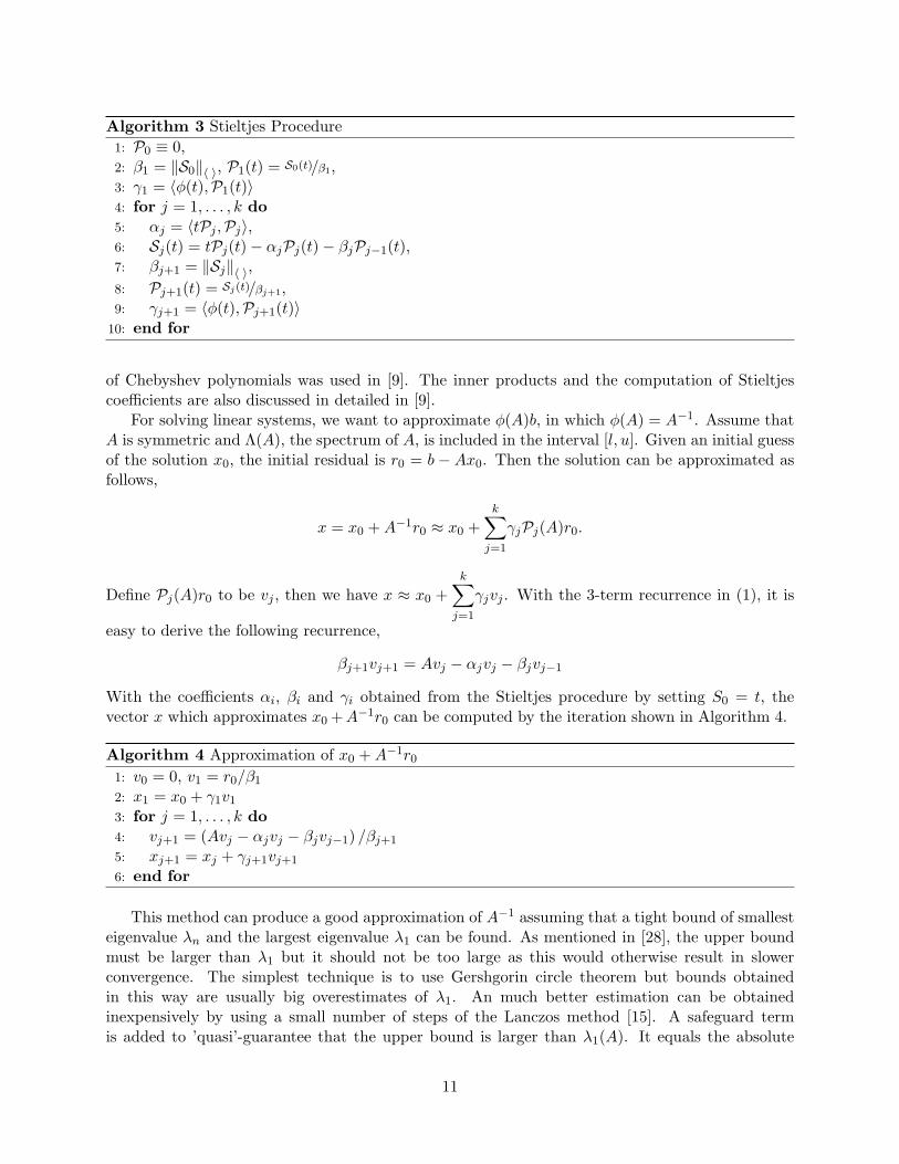
Algorithm 3 Stieltjes Procedure

1: P0 ≡ 0,2: β1 = ‖S0‖〈 〉, P1(t) = S0(t)/β1,3: γ1 = 〈φ(t),P1(t)〉4: for j = 1, . . . , k do

5: αj = 〈tPj ,Pj〉,6: Sj(t) = tPj(t)− αjPj(t)− βjPj−1(t),7: βj+1 = ‖Sj‖〈 〉,

8: Pj+1(t) = Sj(t)/βj+1,9: γj+1 = 〈φ(t),Pj+1(t)〉

10: end for

of Chebyshev polynomials was used in [9]. The inner products and the computation of Stieltjescoefficients are also discussed in detailed in [9].

For solving linear systems, we want to approximate φ(A)b, in which φ(A) = A−1. Assume thatA is symmetric and Λ(A), the spectrum of A, is included in the interval [l, u]. Given an initial guessof the solution x0, the initial residual is r0 = b − Ax0. Then the solution can be approximated asfollows,

x = x0 + A−1r0 ≈ x0 +k

∑

j=1

γjPj(A)r0.

Define Pj(A)r0 to be vj , then we have x ≈ x0 +k

∑

j=1

γjvj . With the 3-term recurrence in (1), it is

easy to derive the following recurrence,

βj+1vj+1 = Avj − αjvj − βjvj−1

With the coefficients αi, βi and γi obtained from the Stieltjes procedure by setting S0 = t, thevector x which approximates x0 + A−1r0 can be computed by the iteration shown in Algorithm 4.

Algorithm 4 Approximation of x0 + A−1r0

1: v0 = 0, v1 = r0/β1

2: x1 = x0 + γ1v1

3: for j = 1, . . . , k do

4: vj+1 = (Avj − αjvj − βjvj−1) /βj+1

5: xj+1 = xj + γj+1vj+1

6: end for

This method can produce a good approximation of A−1 assuming that a tight bound of smallesteigenvalue λn and the largest eigenvalue λ1 can be found. As mentioned in [28], the upper boundmust be larger than λ1 but it should not be too large as this would otherwise result in slowerconvergence. The simplest technique is to use Gershgorin circle theorem but bounds obtainedin this way are usually big overestimates of λ1. An much better estimation can be obtainedinexpensively by using a small number of steps of the Lanczos method [15]. A safeguard termis added to ’quasi’-guarantee that the upper bound is larger than λ1(A). It equals the absolute

11

MATRIX N NNZ NNZ/ROW

sherman3 5,005 20,033 4.0

memplus 17,758 126,150 7.1

msc23052 23,052 588,933 25.6

bcsstk36 23,052 1,143,140 49.6

dubcova2 65,025 547,625 8.4

cfd1 70,656 949,510 13.4

poisson3Db 85,623 2,374,949 27.7

cfd2 123,440 1,605,669 13.0

boneS01 127,224 3,421,188 26.9

majorbasis 160,000 1,750,416 10.9

copcase1 208,340 1,382,902 6.6

af shell8 504,855 9,046,865 17.9

parafem 525,825 2,100,225 4.0

ecology2 999,999 2,997,995 3.0

lap7pt 1,000,000 6,940,000 6.9

spe10 1,094,421 7,598,799 6.9

thermal2 1,228,045 4,904,179 4.0

atmosmodd 1,270,432 8,814,880 6.9

atmosmodl 1,489,752 10,319,760 6.9

Table 3: Matrices used for experiments

value of the last element of the normalized eigenvector associated with the largest eigenvalue of thetridiagonal matrix. This safeguard is not theoretical but is observed to be generally effective[28].The computations in preconditioning operation consists of the SpMV and level-1 BLAS vectoroperations, both of which can be performed efficiently on GPUs. Typically a small number of stepsof Lanczos iterations are enough to provide a good estimate of extreme eigenvalues. The Lanczosalgorithm can be accelerated by GPUs as well, since the computations it required are also SpMVsand level-1 BLAS vector computations.

6 Experiment Results

The experiments were conducted on a workstation with Intel Xeon E5504 Processor (4M Cache, 2.00GHz, 8-core) and an NVIDIA TESLA C1060 GPU (240 cores, 1.3 GHz, 4GB memory) running64-bit Linux system. The CUDA Toolkit and SDK 3.1 are used for programming. The CUDAkernels were compiled by NVIDIA CUDA Compiler (nvcc) with flag -arch sm 13 in order to enabledouble precision. The CPU program is compiled by g++ compiler using -O3 optimization level.

For the iterative linear solves, the stopping criterion for convergence is that the relative residualbe ≤ 10−6. The maximum number of iterations allowed is 1, 000. The linear systems used aretaken from the University of Florida sparse matrix collection [8] and a few cases from reservoirsimulations were also used. The size, number of non-zeros and average number of non-zeros perrow of each matrix are tabulated in Table 3.

12

0

2

4

6

8

10

12

GF

LOP

S

sherm

an3

memplu

s

msc23

052

bcsst

k36

dubc

ova2

cfd1

poiss

on3D

bcfd

2

bone

S01

majorb

asis

copc

ase1

af_sh

ell8

paraf

em

ecolo

gy2

lap7p

t

spe1

0

therm

al2

atmos

modd

atmos

modl

CPU−SerialCPU−ParallelGPU−CSR−ScalarGPU−CSR−VectorGPU−JAD

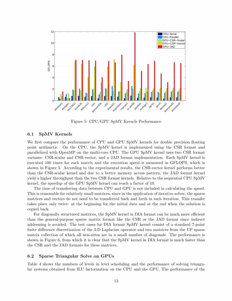
Figure 5: CPU/GPU SpMV Kernels Performance

6.1 SpMV Kernels

We first compare the performance of CPU and GPU SpMV kernels for double precision floatingpoint arithmetic. On the CPU, the SpMV kernel is implemented using the CSR format andparallelized with OpenMP on the multi-core CPU. The GPU SpMV kernel uses two CSR formatvariants: CSR-scalar and CSR-vector, and a JAD format implementation. Each SpMV kernel isexecuted 100 times for each matrix and the execution speed is measured in GFLOPS, which isshown in Figure 5. According to the experimental results, the CSR-vector kernel performs betterthan the CSR-scalar kernel and due to a better memory access pattern, the JAD format kernelyield a higher throughput than the two CSR format kernels. Relative to the sequential CPU SpMVkernel, the speedup of the GPU SpMV kernel can reach a factor of 10.

The time of transferring data between CPU and GPU is not included in calculating the speed.This is reasonable for relatively small matrices, since in the application of iterative solver, the sparsematrices and vectors do not need to be transferred back and forth in each iteration. This transfertakes place only twice: at the beginning for the initial data and at the end when the solution iscopied back.

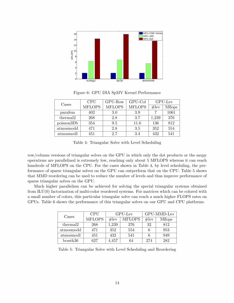
For diagonally structured matrices, the SpMV kernel in DIA format can be much more efficientthan the general-purpose sparse matrix format like the CSR or the JAD format since indirectaddressing is avoided. The test cases for DIA format SpMV kernel consist of a standard 7-pointfinite difference discretization of the 3-D Laplacian operator and two matrices from the UF sparsematrix collection of which all non-zeros are in a small number of diagonals. The performance isshown in Figure 6, from which it is clear that the SpMV kernel in DIA format is much faster thanthe CSR and the JAD formats for these matrices.

6.2 Sparse Triangular Solve on GPUs

Table 4 shows the numbers of levels in level scheduling and the performance of solving triangu-lar systems obtained from ILU factorization on the CPU and the GPU. The performance of the

13

ecology2 lap7pt atmosmodd0

2

4

6

8

10

12

14

16

GF

LOP

S

GPU−CSR−VectorGPU−JADGPU−DIA

Figure 6: GPU DIA SpMV Kernel Performance

CasesCPU GPU-Row GPU-Col GPU-Lev

MFLOPS MFLOPS MFLOPS #lev Mflops

parafem 402 3.0 3.9 7 1061

thermal2 268 2.8 3.7 1,239 376

poisson3Db 354 9.5 11.6 136 812

atmosmodd 471 2.8 3.5 352 554

atmosmodl 451 2.7 3.4 432 541

Table 4: Triangular Solve with Level Scheduling

row/column versions of triangular solves on the GPU in which only the dot products or the saxpyoperations are parallelized is extremely low, reaching only about 5 MFLOPS whereas it can reachhundreds of MFLOPS on the CPU. For the cases shown in Table 4, by level scheduling, the per-formance of sparse triangular solves on the GPU can outperform that on the CPU. Table 5 showsthat MMD reordering can be used to reduce the number of levels and thus improve performance ofsparse triangular solves on the GPU.

Much higher parallelism can be achieved for solving the special triangular systems obtainedfrom ILU(0) factorization of multi-color reordered systems. For matrices which can be colored witha small number of colors, this particular triangular solve can reach a much higher FLOPS rates onGPUs. Table 6 shows the performance of this triangular solves on our GPU and CPU platforms.

CasesCPU GPU-Lev GPU-MMD-Lev

MFLOPS #lev MFLOPS #lev Mflops

thermal2 268 1,239 376 32 812

atmosmodd 471 352 554 6 953

atmosmodl 451 432 541 6 949

bcsstk36 627 4,457 64 274 282

Table 5: Triangular Solve with Level Scheduling and Reordering

14

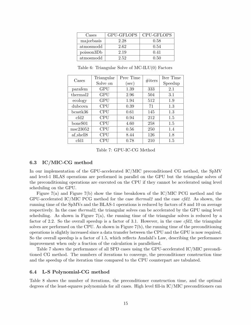
Cases GPU-GFLOPS CPU-GFLOPS

majorbasis 2.28 0.58

atmosmodd 2.62 0.54

poisson3Db 2.19 0.41

atmosmodd 2.52 0.50

Table 6: Triangular Solve of MC-ILU(0) Factors

CasesTriangular Prec Time

#itersIter Time

Solve on (sec) Speedup

parafem GPU 1.39 333 2.1

thermal2 GPU 2.96 504 3.1

ecology GPU 1.94 512 1.9

dubcova CPU 0.39 71 1.3

bcsstk36 CPU 0.61 145 1.3

cfd2 CPU 0.94 212 1.5

boneS01 CPU 4.60 258 1.5

msc23052 CPU 0.56 250 1.4

af shell8 CPU 8.44 126 1.8

cfd1 CPU 0.78 210 1.5

Table 7: GPU-IC-CG Method

6.3 IC/MIC-CG method

In our implementation of the GPU-accelerated IC/MIC preconditioned CG method, the SpMVand level-1 BLAS operations are performed in parallel on the GPU but the triangular solves ofthe preconditioning operations are executed on the CPU if they cannot be accelerated using levelscheduling on the GPU.

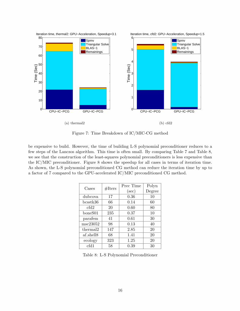
Figure 7(a) and Figure 7(b) show the time breakdown of the IC/MIC PCG method and theGPU-accelerated IC/MIC PCG method for the case thermal2 and the case cfd2. As shown, therunning time of the SpMVs and the BLAS-1 operations is reduced by factors of 8 and 10 on averagerespectively. In the case thermal2, the triangular solves can be accelerated by the GPU using levelscheduling. As shown in Figure 7(a), the running time of the triangular solves is reduced by afactor of 2.2. So the overall speedup is a factor of 3.1. However, in the case cfd2, the triangularsolves are performed on the CPU. As shown in Figure 7(b), the running time of the preconditioningoperations is slightly increased since a data transfer between the CPU and the GPU is now required.So the overall speedup is a factor of 1.5, which reflects Amdahl’s Law, describing the performanceimprovement when only a fraction of the calculation is parallelized.

Table 7 shows the performance of all SPD cases using the GPU-accelerated IC/MIC precondi-tioned CG method. The numbers of iterations to converge, the preconditioner construction timeand the speedup of the iteration time compared to the CPU counterpart are tabulated.

6.4 L-S Polynomial-CG method

Table 8 shows the number of iterations, the preconditioner construction time, and the optimaldegrees of the least-squares polynomials for all cases. High level fill-in IC/MIC preconditioners can

15

CPU−IC−PCG GPU−IC−PCG0

10

20

30

40

50

60

70

80T

ime

(Sec

)Iteration time, thermal2: GPU−Acceleration, Speedup=3.1

SpmvTriangular SolveBLAS−1Remainings

(a) thermal2

CPU−IC−PCG GPU−IC−PCG0

1

2

3

4

5

6

Tim

e (S

ec)

Iteration time, cfd2: GPU−Acceleration, Speedup=1.5

SpmvTriangular SolveBLAS−1Remainings

(b) cfd2

Figure 7: Time Breakdown of IC/MIC-CG method

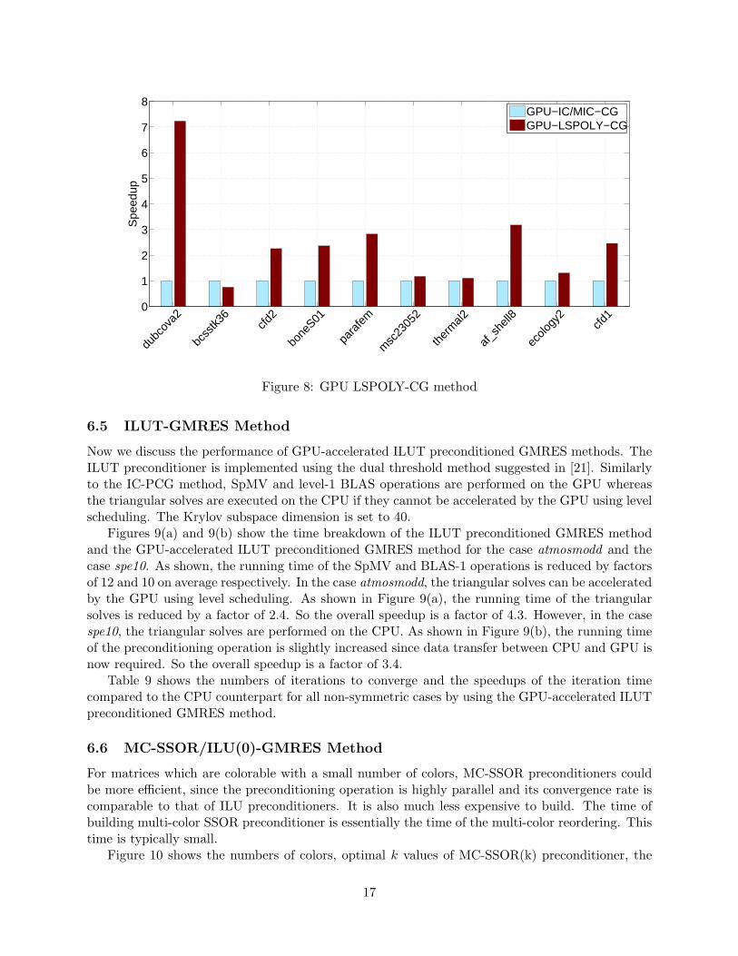
be expensive to build. However, the time of building L-S polynomial preconditioner reduces to afew steps of the Lanczos algorithm. This time is often small. By comparing Table 7 and Table 8,we see that the construction of the least-squares polynomial preconditioners is less expensive thanthe IC/MIC preconditioner. Figure 8 shows the speedup for all cases in terms of iteration time.As shown, the L-S polynomial preconditioned CG method can reduce the iteration time by up toa factor of 7 compared to the GPU-accelerated IC/MIC preconditioned CG method.

Cases #ItersPrec Time Polyn

(sec) Degree

dubcova 17 0.36 10

bcsstk36 66 0.14 60

cfd2 20 0.60 80

boneS01 235 0.37 10

parafem 41 0.61 30

msc23052 98 0.13 40

thermal2 147 2.85 20

af shell8 68 1.41 20

ecology 323 1.25 20

cfd1 58 0.39 30

Table 8: L-S Polynomial Preconditioner

16

0

1

2

3

4

5

6

7

8

Spe

edup

dubc

ova2

bcss

tk36

cfd2

bone

S01

para

fem

msc

2305

2

ther

mal2

af_s

hell8

ecolo

gy2

cfd1

GPU−IC/MIC−CGGPU−LSPOLY−CG

Figure 8: GPU LSPOLY-CG method

6.5 ILUT-GMRES Method

Now we discuss the performance of GPU-accelerated ILUT preconditioned GMRES methods. TheILUT preconditioner is implemented using the dual threshold method suggested in [21]. Similarlyto the IC-PCG method, SpMV and level-1 BLAS operations are performed on the GPU whereasthe triangular solves are executed on the CPU if they cannot be accelerated by the GPU using levelscheduling. The Krylov subspace dimension is set to 40.

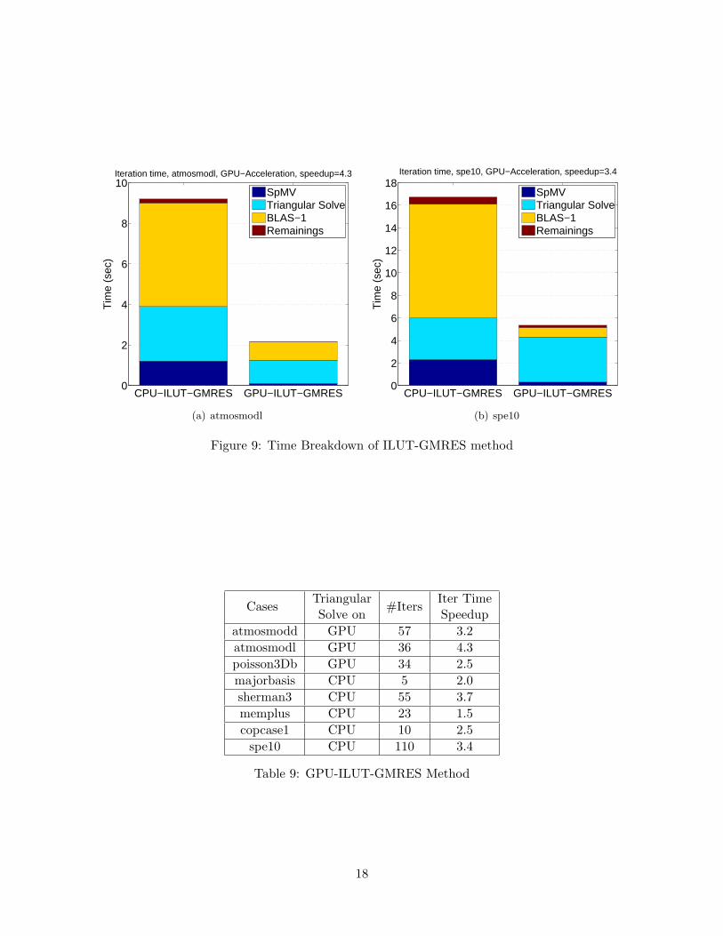
Figures 9(a) and 9(b) show the time breakdown of the ILUT preconditioned GMRES methodand the GPU-accelerated ILUT preconditioned GMRES method for the case atmosmodd and thecase spe10. As shown, the running time of the SpMV and BLAS-1 operations is reduced by factorsof 12 and 10 on average respectively. In the case atmosmodd, the triangular solves can be acceleratedby the GPU using level scheduling. As shown in Figure 9(a), the running time of the triangularsolves is reduced by a factor of 2.4. So the overall speedup is a factor of 4.3. However, in the casespe10, the triangular solves are performed on the CPU. As shown in Figure 9(b), the running timeof the preconditioning operation is slightly increased since data transfer between CPU and GPU isnow required. So the overall speedup is a factor of 3.4.

Table 9 shows the numbers of iterations to converge and the speedups of the iteration timecompared to the CPU counterpart for all non-symmetric cases by using the GPU-accelerated ILUTpreconditioned GMRES method.

6.6 MC-SSOR/ILU(0)-GMRES Method

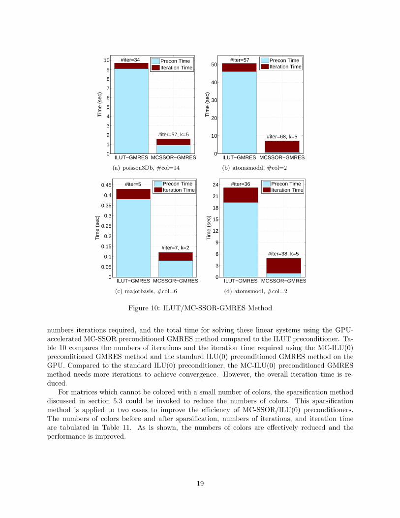
For matrices which are colorable with a small number of colors, MC-SSOR preconditioners couldbe more efficient, since the preconditioning operation is highly parallel and its convergence rate iscomparable to that of ILU preconditioners. It is also much less expensive to build. The time ofbuilding multi-color SSOR preconditioner is essentially the time of the multi-color reordering. Thistime is typically small.

Figure 10 shows the numbers of colors, optimal k values of MC-SSOR(k) preconditioner, the

17

CPU−ILUT−GMRES GPU−ILUT−GMRES0

2

4

6

8

10

Tim

e (s

ec)

Iteration time, atmosmodl, GPU−Acceleration, speedup=4.3

SpMVTriangular SolveBLAS−1Remainings

(a) atmosmodl

CPU−ILUT−GMRES GPU−ILUT−GMRES0

2

4

6

8

10

12

14

16

18

Tim

e (s

ec)

Iteration time, spe10, GPU−Acceleration, speedup=3.4

SpMVTriangular SolveBLAS−1Remainings

(b) spe10

Figure 9: Time Breakdown of ILUT-GMRES method

CasesTriangular

#ItersIter Time

Solve on Speedup

atmosmodd GPU 57 3.2

atmosmodl GPU 36 4.3

poisson3Db GPU 34 2.5

majorbasis CPU 5 2.0

sherman3 CPU 55 3.7

memplus CPU 23 1.5

copcase1 CPU 10 2.5

spe10 CPU 110 3.4

Table 9: GPU-ILUT-GMRES Method

18

ILUT−GMRES MCSSOR−GMRES0

1

2

3

4

5

6

7

8

9

10

Tim

e (s

ec)

Precon TimeIteration Time

#iter=57, k=5

#iter=34

(a) poisson3Db, #col=14

ILUT−GMRES MCSSOR−GMRES0

10

20

30

40

50

Tim

e (s

ec)

Precon TimeIteration Time

#iter=57

#iter=68, k=5

(b) atomsmodd, #col=2

ILUT−GMRES MCSSOR−GMRES0

0.05

0.1

0.15

0.2

0.25

0.3

0.35

0.4

0.45

Tim

e (s

ec)

Precon TimeIteration Time

#iter=7, k=2

#iter=5

(c) majorbasis, #col=6

ILUT−GMRES MCSSOR−GMRES0

3

6

9

12

15

18

21

24

Tim

e (s

ec)

Precon TimeIteration Time

#iter=36

#iter=38, k=5

(d) atomsmodl, #col=2

Figure 10: ILUT/MC-SSOR-GMRES Method

numbers iterations required, and the total time for solving these linear systems using the GPU-accelerated MC-SSOR preconditioned GMRES method compared to the ILUT preconditioner. Ta-ble 10 compares the numbers of iterations and the iteration time required using the MC-ILU(0)preconditioned GMRES method and the standard ILU(0) preconditioned GMRES method on theGPU. Compared to the standard ILU(0) preconditioner, the MC-ILU(0) preconditioned GMRESmethod needs more iterations to achieve convergence. However, the overall iteration time is re-duced.

For matrices which cannot be colored with a small number of colors, the sparsification methoddiscussed in section 5.3 could be invoked to reduce the numbers of colors. This sparsificationmethod is applied to two cases to improve the efficiency of MC-SSOR/ILU(0) preconditioners.The numbers of colors before and after sparsification, numbers of iterations, and iteration timeare tabulated in Table 11. As is shown, the numbers of colors are effectively reduced and theperformance is improved.

19

CasesMC-ILU(0) ILU(0)

#iters Iter Time #iters Iter Time

poisson3Db 96 0.53 96 0.85

atomsmodd 219 5.32 176 7.94

majorbasis 12 0.04 9 0.07

atomsmodl 96 2.66 58 3.00

Table 10: ILU(0)/MC-ILU(0)-GMRES Method

Cases Precon Sparsify #col #iter Time

memplusMC-SSOR

No 22 47 0.23Yes 3 32 0.07

MC-ILU(0)No 22 104 0.35Yes 3 115 0.20

spe10MC-SSOR

No 340 202 28.14Yes 5 200 10.88

MC-ILU(0)No 340 559 29.05Yes 53 607 22.31

Table 11: MC-SSOR/ILU(0) with Sparsification

6.7 Block Jacobi-GMRES Method

When using block Jacobi preconditioning, matrices are first partitioned by some graph partitioningalgorithm like METIS [14] and reordered. Then ILUT factorization is performed on each diagonalblock. The preconditioning operation, the block L/U solves are executed on the GPU. As shown inFigure 11(a), the speed of the Block L/U solve is increased as the number of blocks grows, becausemore parallelism is available in the computation. However, as shown in Figure 11(b), the numberof iterations required increases. The iteration time is shown in Figure 11(c).

Table 12 shows the performance of PCG methods for solving a 2D/3D Poisson equation. Thefirst row of Table 12 shows the IC/MIC preconditioned CG method running on the CPU. Row 2 torow 7 show the GPU-accelerated PCG methods with different preconditioners. By comparing therows of Table 12, we can see that the GPU-acceleration in the PCG methods and the performancedifference between different preconditioners.

PreconLap2d Lap3d

#iters time(sec) #iters time(sec)

CPU-IC 94 2.24 48 4.40

GPU-IC 94 1.14 48 2.14

GPU-LS-POLY 55 0.85 16 0.90

GPU-IC(0) 254 1.91 80 2.04

GPU-MC-IC(0) 442 1.12 129 1.15

GPU-MC-SSOR 309 1.83 104 2.25

GPU-BJ 251 2.27 95 2.73

Table 12: Performance Comparison of All Preconditioning

20

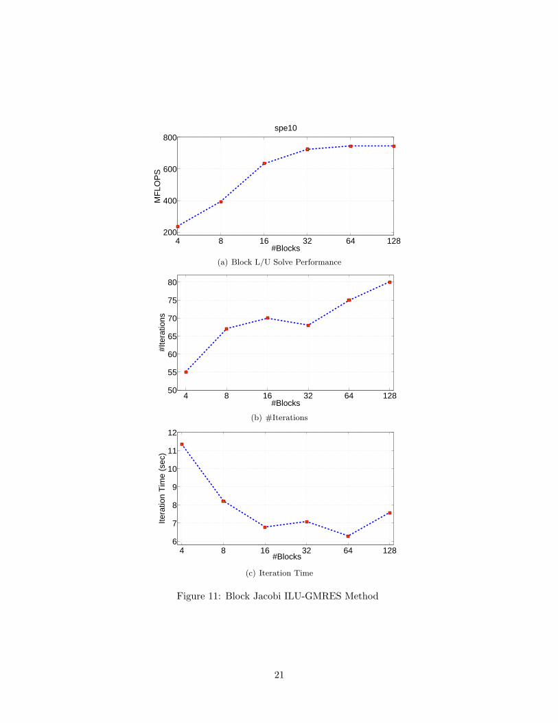
4 8 16 32 64 128200

400

600

800spe10

#Blocks

MF

LOP

S

(a) Block L/U Solve Performance

4 8 16 32 64 12850

55

60

65

70

75

80

#Blocks

#Ite

ratio

ns

(b) #Iterations

4 8 16 32 64 1286

7

8

9

10

11

12

#Blocks

Itera

tion

Tim

e (s

ec)

(c) Iteration Time

Figure 11: Block Jacobi ILU-GMRES Method

21

7 Conclusion

In this work, we have explored high performance sparse matrix-vector product (SpMV) kernelsin different formats on current many-core platforms and used them to construct effective iterativelinear solvers with several preconditioner options. Since the performance of triangular solve is low onGPUs, this computation can be accomplished by CPUs. By this hybrid CPU/GPU computations,IC preconditioned CG method and ILU preconditioned GMRES method are adapted to a GPUenvironment and achieve performance gains compared to its CPU counterpart. In order to achievebetter GPU-acceleration, a few preconditioners with enhanced parellelism were considered. Amongthese, the block Jacobi preconditioner is the simplest but it is usually not efficient since it requiresmany iterations to converge. For matrices which can be colored with a small number of colors, multi-color SSOR/ILU(0) preconditioners could provide a better performance since their preconditioningoperations can be executed with high parallelism and they can yield comparable convergence ratesto the standard ILU preconditioners. For symmetric linear systems, the Least-Squares polynomialpreconditioner can be much more efficient for the PCG method since its preconditioning operationrelies on the SpMV kernel.

Based on the experimental results reported here and elsewhere, we observe that, when used asgeneral purpose many-core processors, current GPUs provide a much lower performance advantagefor irregular (sparse) computations than they can for more regular (dense) computations. However,when used carefully, GPUs can still be beneficial as co-processors to CPUs to speed-up complexcomputations. We highlighted a few alternative approaches to standard ones in the arena of iterativesparse linear system solvers.

In our future work we will take a more careful look of the GPU SpMV kernels using CUDA VisualProfiler to find the potential throughput bottleneck. We will also consider the hybrid format SpMVkernel suggested in [5] and explore more efficient preconditioning techniques for GPU-acceleratediterative linear solvers.

References

[1] Anant Agarwal and Markus Levy, The kill rule for multicore, DAC ’07: Proceedings of the44th annual Design Automation Conference (New York, NY, USA), ACM, 2007, pp. 750–753.

[2] Emmanuel Agullo, Jim Demmel, Jack Dongarra, Bilel Hadri, Jakub Kurzak, Julien Langou,Hatem Ltaief, Piotr Luszczek, and Stanimire Tomov, Numerical linear algebra on emerging

architectures: The PLASMA and MAGMA projects, Journal of Physics: Conference Series180 (2009), no. 1, 012037.

[3] Marco Ament, Gunter Knittel, Daniel Weiskopf, and Wolfgang Strasser, A parallel precondi-

tioned conjugate gradient solver for the poisson problem on a multi-gpu platform, PDP ’10:Proceedings of the 2010 18th Euromicro Conference on Parallel, Distributed and Network-based Processing (Washington, DC, USA), IEEE Computer Society, 2010, pp. 583–592.

[4] Muthu Manikandan Baskaran and Rajesh Bordawekar, Optimizing sparse matrix-vector mul-

tiplication on GPUs, Tech. report, IBM Research, 2008.

[5] Nathan Bell and Michael Garland, Implementing sparse matrix-vector multiplication on

throughput-oriented processors, SC ’09: Proceedings of the Conference on High PerformanceComputing Networking, Storage and Analysis (New York, NY, USA), ACM, 2009, pp. 1–11.

22

[6] Jeff Bolz, Ian Farmer, Eitan Grinspun, and Peter Schrooder, Sparse matrix solvers on the gpu:

conjugate gradients and multigrid, ACM Trans. Graph. 22 (2003), no. 3, 917–924.

[7] Philip J. Davis, Interpolation and approximation, Blaisdell, Waltham, MA, 1963.

[8] Timothy A. Davis, University of florida sparse matrix collection, na digest, 1994.

[9] J. Erhel, F. Guyomarc, and Y. Saad, Least-squares polynomial filters for ill-conditioned lin-

ear systems, Tech. Report umsi-2001-32, Minnesota Supercomputer Institute, University ofMinnesota, Minneapolis, MN, 2001.

[10] F.Vazquez, E.M.Garzon, J.A.Martinez, and J.J.Fernandez, The sparse matrix vector product

on GPUs, Tech. report, Dept of Computer Architecture and Electronics, University of Almeria,2009.

[11] A. George and W. H. Liu, The evolution of the minimum degree ordering algorithm, SIAMRev. 31 (1989), no. 1, 1–19.

[12] Serban Georgescu and Hiroshi Okuda, Conjugate gradients on graphic hardware: Performance

& Feasibility, 2007.

[13] Rohit Gupta, A GPU implementation of a bubbly flow solver , Master’s thesis, Delft Instituteof Applied Mathematics, Delft University of Technology, 2628 BL Delft, The Netherlands,2009.

[14] George Karypis and Vipin Kumar, Metis - a software package for partitioning unstructured

graphs, partitioning meshes, and computing fill-reducing orderings of sparse matrices, version

4.0, Tech. report, University of Minnesota, Department of Computer Science / Army HPCResearch Center, 1998.

[15] C. Lanczos, An iteration method for the solution of the eigenvalue problem of linear differential

and integral operators, Journal of Research of the National Bureau of Standards 45 (1950),255–282.

[16] Ruipeng Li, Hector Klie, Hari Sudan, and Yousef Saad, Towards realistic reservoir simulations

on manycore platforms, SPE Journal (2010), 1–23, submitted.

[17] NVIDIA, Cublas library user guide 3.0, 2010.

[18] , NVIDIA CUDA programming guide 3.0, 2010.

[19] Yves Robert, Regular incomplete factorizations of real positive definite matrices, Linear Alge-bra and its Applications 48 (1982), 105 – 117.

[20] Y. Saad, SPARSKIT: A basic tool kit for sparse matrix computations, Tech. Report RIACS-90-20, Research Institute for Advanced Computer Science, NASA Ames Research Center, MoffettField, CA, 1990.

[21] , ILUT: a dual threshold incomplete ILU factorization, Numerical Linear Algebra withApplications 1 (1994), 387–402.

[22] , Iterative methods for sparse linear systems, 2nd edition, SIAM, Philadelpha, PA, 2003.

23

[23] Y. Saad and M. H. Schultz, GMRES: a generalized minimal residual algorithm for solving

nonsymmetric linear systems, SIAM Journal on Scientific and Statistical Computing 7 (1986),856–869.

[24] Shubhabrata Sengupta, Mark Harris, Yao Zhang, and John D. Owens, Scan primitives for gpu

computing, Graphics Hardware 2007, ACM, August 2007, pp. 97–106.

[25] H. Sudan, H. Klie, R. Li, and Y. Saad, High performance manycore solvers for reservoir

simulation, 12th European Conference on the Mathematics of Oil Recovery, 2010.

[26] Vasily Volkov and James Demmel, LU, QR and Cholesky factorizations using vector capabilities

of GPUs, Tech. report, Computer Science Division University of California at Berkeley, 2008.

[27] Mingliang Wang, Hector Klie, Manish Parashar, and Hari Sudan, Solving sparse linear systems

on nvidia tesla gpus, ICCS ’09: Proceedings of the 9th International Conference on Computa-tional Science (Berlin, Heidelberg), Springer-Verlag, 2009, pp. 864–873.

[28] Yunkai Zhou, Yousef Saad, Murilo L. Tiago, and James R. Chelikowsky, Parallel self-

consistent-field calculations via Chebyshev-filtered subspace acceleration, Phy. rev. E 74 (2006),066704.

24