Embed Size (px)
Citation preview

March 18-21, 2013 | San Jose, California
GPU Technology Conference 2013
GPU-Based Real-Time SAS Processing On-Board Autonomous
Underwater Vehicles
Jesús Ortiz Advanced Robotics Department (ADVR)
Istituto Italiano di tecnologia (IIT)
Francesco Baralli
Center for Maritime Research and Experimentation (CMRE) NATO Science and Technology Organization (STO)

GPU Technology Conference March 18-21, 2013 | San Jose, California 2
NATO Science and Technology Organization
Center for Maritime Research and Experimentation
• Within the framework of the STO, CMRE organizes and conducts scientific
research and technology development, and delivers innovative and field-tested S&T solutions to address the defense and security needs of the Alliance.
• The CMRE is customer funded. Customers will be comprised of NATO bodies, NATO Nations and other parties, consistent with NATO policy.
• The mission of the CMRE is centered on the maritime domain, but may extrapolate into other domains to meet customers’ demands.
• CMRE maintains a set of core technical capabilities, including: underwater acoustics, sensors and signal processing, autonomy, ocean engineering, seagoing capability, and AUVs.
CMRE@NATO STO Overview

GPU Technology Conference March 18-21, 2013 | San Jose, California 3
Istituto Italiano di Tecnologia
Advanced Robotics Department
• Innovative and multidisciplinary approach to humanoid design and control, and the development of novel robotic components and technologies: – Hardware: mechanical/ electrical design and fabrication, sensor systems, actuation
development, etc.
– Software: control, computer software, human factors, etc.
• Transition from traditional (hard-bodied) robots towards a new generation of hybrid systems (biologically inspired concepts: muscle, bone, tendon, skin…)
• Research activities: – core scientific/technological research aimed at providing fundamental competencies needed to
develop robotic and humanoid technology
– advanced research demonstrators that provide large focused research projects integrating the core sciences
ADVR@IIT Overview

GPU Technology Conference March 18-21, 2013 | San Jose, California 4
• Basic: – Perform underwater missions following pre-programmed path
– No human operator in the control loop
– Carry different sets of environmental and/or imaging sensors
– Communicate with surface station and with other agents
• Advanced – Real-time data processing and analysis
– High level of autonomy: adaptive behavior
– Cooperative behavior among different AUVs
Autonomous Underwater Vehicle (AUV)

GPU Technology Conference March 18-21, 2013 | San Jose, California 5
Synthetic Aperture Sonar (SAS): – Multiple pulses to create a
large synthetic array (aperture)
– One pixel of the image is produced using information from multiple pulses
– Multistatic approach (one emitter, multiple receivers)
– The emitted ping is a “chirp” (broad frequency band)
Sonar Imaging
Pings
Ran
ge

GPU Technology Conference March 18-21, 2013 | San Jose, California 6
• Sonar on both sides (port & starboard)
• Two receiver arrays per side:
– Main array (36 elements)
– Bathymetric array (12 elements)
AUV
Surge (longitudinal, along-track)
Sway (lateral,
cross-track, range)
Yaw (heading,
North)
Roll
Pitch
Heave (Depth, vertical)

GPU Technology Conference March 18-21, 2013 | San Jose, California 7
Synthetic Aperture Sonar (SAS)
Port side
Starboard side
Along-track (movement)
Range (cross-track)
Range (cross-track)

GPU Technology Conference March 18-21, 2013 | San Jose, California 8
SAS result
GPU Technology Conference March 18-21, 2013 | San Jose, California 9
• Preprocessing (calibration & matching)
• Displaced Phase Center Antenna (DPCA)
• Navigation Integration
• SAS imaging
• SAS Interferometry 3D images
Automatic Target Recognition (ATR)
Replanning
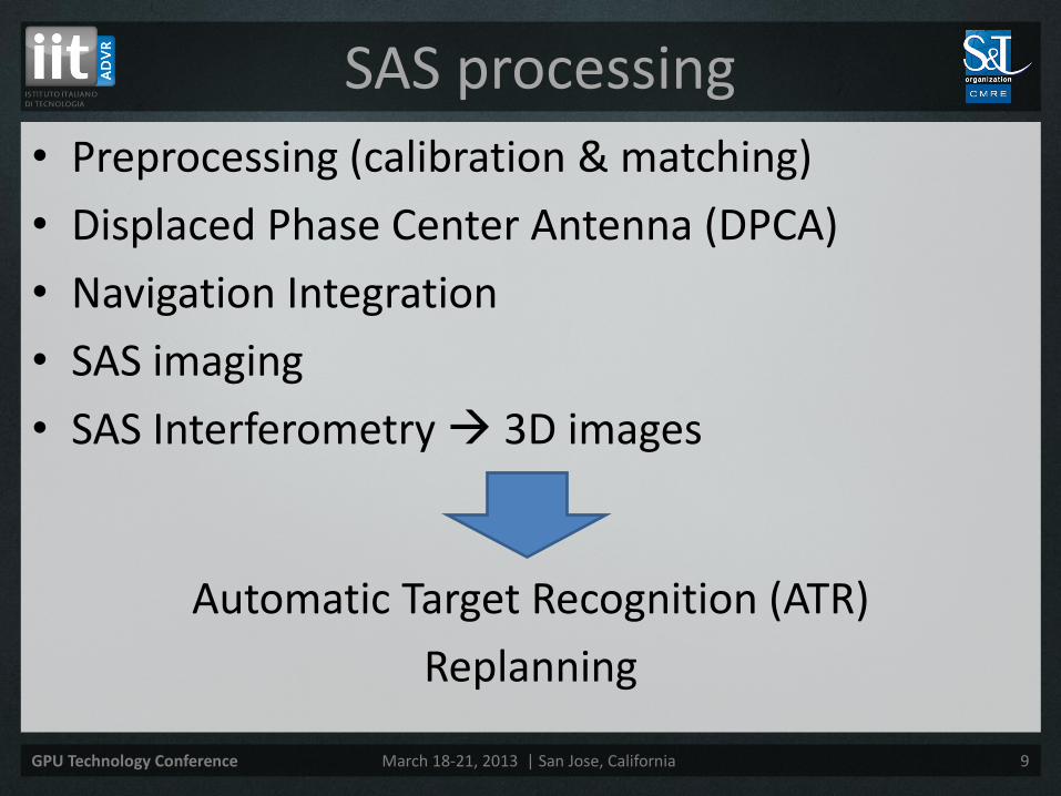
SAS processing

GPU Technology Conference March 18-21, 2013 | San Jose, California 10
• Preprocessing (calibration & matching)
• Displaced Phase Center Antenna (DPCA)
• Navigation Integration
• SAS imaging
• SAS Interferometry 3D images
Automatic Target Recognition (ATR)
Replanning
SAS processing
GPU Technology Conference March 18-21, 2013 | San Jose, California 11
SAS processing
PING 1
Preprocessing
PING 2
Preprocessing
DPCA
Motion
SAS Imaging
PING 3
Preprocessing
DPCA
Motion
SAS Imaging
PING N
Preprocessing
DPCA
Motion
SAS Imaging
Stacking tiles
Time (4Hz – 250 ms per ping)
. . .

GPU Technology Conference March 18-21, 2013 | San Jose, California 12
SAS processing
PING 1
Preprocessing
PING 2
Preprocessing
DPCA
Motion
SAS Imaging
PING 3
Preprocessing
DPCA
Motion
SAS Imaging
PING N
Preprocessing
DPCA
Motion
SAS Imaging
Stacking tiles
Time (4Hz – 250 ms per ping)
. . .

GPU Technology Conference March 18-21, 2013 | San Jose, California 13
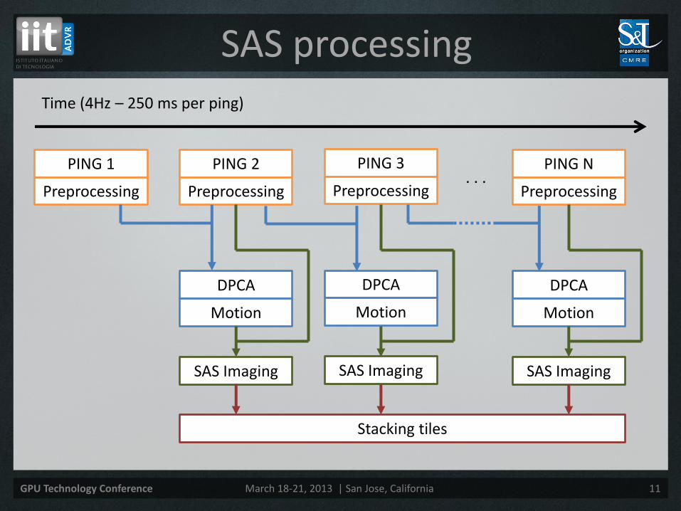
Preprocessing
Read Replica
Replica
FFT
Replica Freq.
Read Ping
Ping
FFT
Replica Shaded
Shading
Copy to Device Copy to Device Copy to Device
Replica Freq. Replica Shaded Ping
Calibration
FFT Multiply Multiply
Inverse FFT Inverse FFT
Matched Ping Shaded Ping
CPU operation
GPU operation
Data in host
Data in device
Only once
Memory transf.
GPU Technology Conference March 18-21, 2013 | San Jose, California 14
Preprocessing
Read Replica
Replica
FFT
Replica Freq.
Read Ping
Ping
FFT
Replica Shaded
Shading
Copy to Device Copy to Device Copy to Device
Replica Freq. Replica Shaded Ping
Calibration
FFT Multiply Multiply
Inverse FFT Inverse FFT
Matched Ping Shaded Ping
CPU operation
GPU operation
Data in host
Data in device
Only once
Memory transf.

GPU Technology Conference March 18-21, 2013 | San Jose, California 15
• Calibrate acoustic data
– Adjust the phase of each receiver due to wiring and reading delays
where:
• 𝐴𝑐 is the calibrated Acoustic data (complex)
• 𝐴𝑟 is the raw Acoustic data (complex)
• 𝐶 is the Calibration (complex of modulus 1)
Preprocessing - Calibration
𝐴𝑐 = 𝐴𝑟 ∙ 𝐶 ⇒ 𝐴𝑐𝑟 = 𝐴𝑟
𝑟 ∙ 𝐶𝑟 − 𝐴𝑟𝑖 ∙ 𝐶𝑖
𝐴𝑐𝑖 = 𝐴𝑟
𝑟 ∙ 𝐶𝑖 + 𝐴𝑟𝑖 ∙ 𝐶𝑟

GPU Technology Conference March 18-21, 2013 | San Jose, California 16
Preprocessing
Read Replica
Replica
FFT
Replica Freq.
Read Ping
Ping
FFT
Replica Shaded
Shading
Copy to Device Copy to Device Copy to Device
Replica Freq. Replica Shaded Ping
Calibration
FFT Multiply Multiply
Inverse FFT Inverse FFT
Matched Ping Shaded Ping
CPU operation
GPU operation
Data in host
Data in device
Only once
Memory transf.

GPU Technology Conference March 18-21, 2013 | San Jose, California 17
• Match acoustic data with the replica
– Unshaded replica For DPCA
– Shaded replica For Imaging
where:
• 𝐴𝑚𝑢 is the Unshaded Matched Acoustic data (complex)
• 𝐴𝑚𝑠 is the Shaded Matched Acoustic data (complex)
• 𝑅𝑢 is the Unshaded Replica (complex)
• 𝑅𝑠 is the Shaded Replica (complex)
Preprocessing - Matching
𝐴𝑚𝑢 = 𝐴𝑐 ∙ 𝑅𝑢
𝐴𝑚𝑠 = 𝐴𝑐 ∙ 𝑅𝑠

GPU Technology Conference March 18-21, 2013 | San Jose, California 18
• Calibration done in place to reduce the memory requirements
• FFT with FFTW (CPU) and cuFFT (GPU)
Preprocessing - Results
CPU1 GPU2 Speedup
84.3 ms 3.7 ms x23
1 Running on an Intel Core i7-920 @ 2.67 GHz 2 Running on a NVIDIA Tesla C1060

GPU Technology Conference March 18-21, 2013 | San Jose, California 19
SAS processing
PING 1
Preprocessing
PING 2
Preprocessing
DPCA
Motion
SAS Imaging
PING 3
Preprocessing
DPCA
Motion
SAS Imaging
PING N
Preprocessing
DPCA
Motion
SAS Imaging
Stacking tiles
Time (4Hz – 250 ms per ping)
. . .

GPU Technology Conference March 18-21, 2013 | San Jose, California 20
Phase Center Approximation
Tx
Rx
PCA
d
d/2

GPU Technology Conference March 18-21, 2013 | San Jose, California 21
DPCA concept
R. Heremans, A. Bellettini and M. Pinto, “Milestone: Displaced Phase Center Array”, September 2006, http://www.sic.rma.ac.be/~rhereman/milestones/dpca.pdf
d
(N-M)·d
N·d
(N-M)·d D=M·d/2
Ping (P)
Ping (P+1)
D AUV displacement d Separation elements N Number of elements K=(N-M) Number of overlapped elements

GPU Technology Conference March 18-21, 2013 | San Jose, California 22
• Find best correlation between consecutive pings
– Use INS for first approximation of surge
– Get best correlation surge correction
– Get delay sway calculation
– Use INS for other variables (roll, pitch, yaw)
DPCA calculation
K overlapped elements K+1 overlapped elements K-1 overlapped elements
tim
e-s
amp
les
Receiver elements

GPU Technology Conference March 18-21, 2013 | San Jose, California 23
• INS information:
– Speed surge estimation
– Accelerometer pitch & roll
– Compass yaw
– Depth heave
• DPCA:
– Surge correction
– Sway calculation
Motion Estimation
Surge (longitudinal, along-track)
Sway (lateral,
cross-track, range)
Yaw (heading,
North)
Roll
Pitch
Heave (Depth, vertical)
GPU Technology Conference March 18-21, 2013 | San Jose, California 24
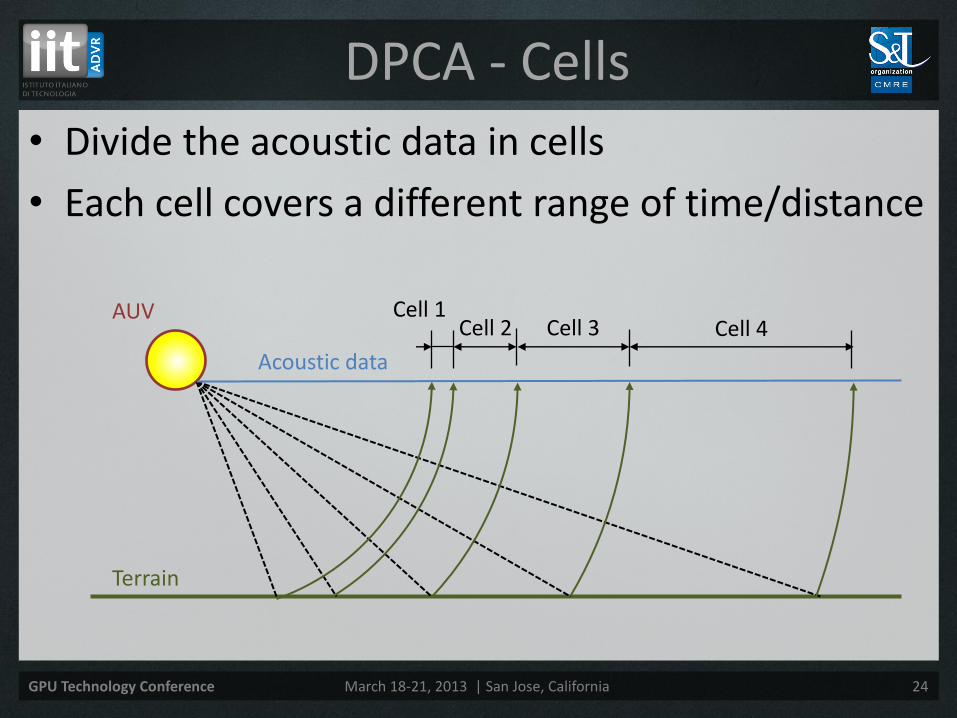
• Divide the acoustic data in cells
• Each cell covers a different range of time/distance
DPCA - Cells
Cell 1 Cell 2 Cell 3 Cell 4
Acoustic data
Terrain
AUV

GPU Technology Conference March 18-21, 2013 | San Jose, California 25
DPCA Processing
For each cell
Copy to cell
Matched Ping Previous
Beamforming
FFT
Normalize
Fourier Interpolation
Scale
Inverse FFT
Matched Ping Current
Copy to cell
FFT
Normalize
Calculate maxima
Shift data
FFT
Shift data
Inverse FFT
Scale
Copy to Host
Maxima
Navigation
DPCA results: Surge, sway,
roll, pitch, yaw, correlation
factor, transmitter
and receiver position, etc
CPU operation
GPU operation
Data in host
Data in device
Memory transf.

GPU Technology Conference March 18-21, 2013 | San Jose, California 26
DPCA Processing
For each cell
Copy to cell
Matched Ping Previous
Beamforming
FFT
Normalize
Fourier Interpolation
Scale
Inverse FFT
Matched Ping Current
Copy to cell
FFT
Normalize
Calculate maxima
Shift data
FFT
Shift data
Inverse FFT
Scale
Copy to Host
Maxima
Navigation
DPCA results: Surge, sway,
roll, pitch, yaw, correlation
factor, transmitter
and receiver position, etc
CPU operation
GPU operation
Data in host
Data in device
Memory transf.
GPU Technology Conference March 18-21, 2013 | San Jose, California 27
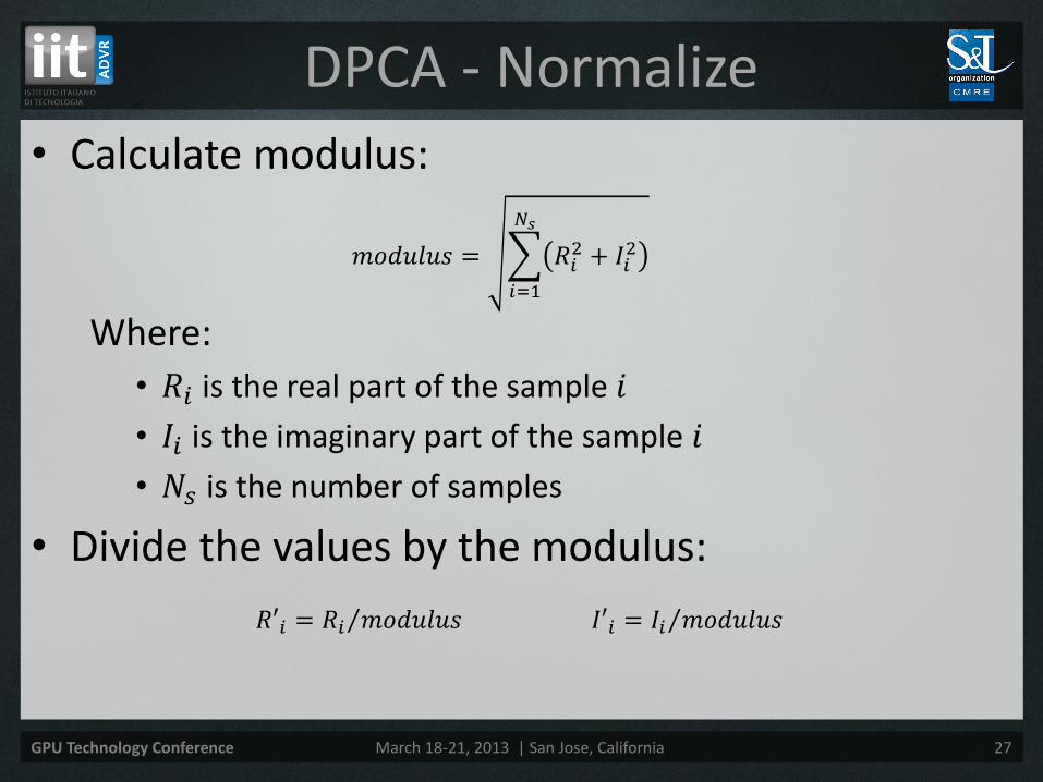
• Calculate modulus:
Where:
• 𝑅𝑖 is the real part of the sample 𝑖
• 𝐼𝑖 is the imaginary part of the sample 𝑖
• 𝑁𝑠 is the number of samples
• Divide the values by the modulus:
DPCA - Normalize
𝑚𝑜𝑑𝑢𝑙𝑢𝑠 = 𝑅𝑖2 + 𝐼𝑖
2
𝑁𝑠
𝑖=1
𝑅′𝑖 = 𝑅𝑖 𝑚𝑜𝑑𝑢𝑙𝑢𝑠 𝐼′𝑖 = 𝐼𝑖 𝑚𝑜𝑑𝑢𝑙𝑢𝑠

GPU Technology Conference March 18-21, 2013 | San Jose, California 28
• Calculate the modulus of each sample
• Each thread calculates more than one sample
where:
• 𝑚𝑜𝑑𝑢𝑙𝑢𝑠𝑡2 is the partial modulus calculated by the thread 𝑡
• 𝑁𝑠𝑡 is the number of samples per thread
• Save the partial modulus in the shared memory
DPCA - Normalize
𝑚𝑜𝑑𝑢𝑙𝑢𝑠𝑡2 = 𝑅𝑖
2 + 𝐼𝑖2
(𝑡+1)∙𝑁𝑠𝑡
𝑖=𝑡∙𝑁𝑠𝑡+1

GPU Technology Conference March 18-21, 2013 | San Jose, California 29
• Calculate the total modulus using a tree
DPCA - Normalize
1 2 3 4 5 6 7 8
1 2 3 4
1 2
1
1 2 3 4
1 2
__syncthreads();
if (threadIdx.x < 128)
modulus[threadIdx.x] += modulus[threadIdx.x + 128];
__syncthreads();
if (threadIdx.x < 64)
modulus[threadIdx.x] += modulus[threadIdx.x + 64];
__syncthreads();
...
__syncthreads();
if (threadIdx.x < 2)
modulus[threadIdx.x] += modulus[threadIdx.x + 2];
__syncthreads();
if (threadIdx.x == 0)
modulus[threadIdx.x] += modulus[threadIdx.x + 1];
__syncthreads();

GPU Technology Conference March 18-21, 2013 | San Jose, California 30
DPCA Processing
For each cell
Copy to cell
Matched Ping Previous
Beamforming
FFT
Normalize
Fourier Interpolation
Scale
Inverse FFT
Matched Ping Current
Copy to cell
FFT
Normalize
Calculate maxima
Shift data
FFT
Shift data
Inverse FFT
Scale
Copy to Host
Maxima
Navigation
DPCA results: Surge, sway,
roll, pitch, yaw, correlation
factor, transmitter
and receiver position, etc
CPU operation
GPU operation
Data in host
Data in device
Memory transf.
GPU Technology Conference March 18-21, 2013 | San Jose, California 31
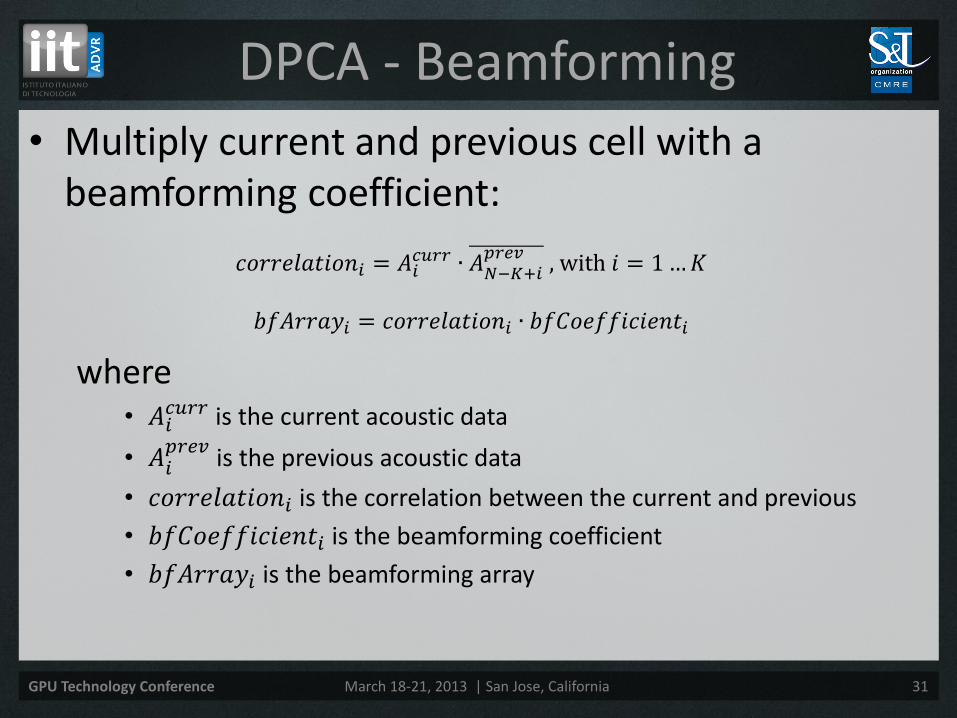
• Multiply current and previous cell with a beamforming coefficient:
where • 𝐴𝑖
𝑐𝑢𝑟𝑟 is the current acoustic data
• 𝐴𝑖𝑝𝑟𝑒𝑣
is the previous acoustic data
• 𝑐𝑜𝑟𝑟𝑒𝑙𝑎𝑡𝑖𝑜𝑛𝑖 is the correlation between the current and previous
• 𝑏𝑓𝐶𝑜𝑒𝑓𝑓𝑖𝑐𝑖𝑒𝑛𝑡𝑖 is the beamforming coefficient
• 𝑏𝑓𝐴𝑟𝑟𝑎𝑦𝑖 is the beamforming array
DPCA - Beamforming
𝑐𝑜𝑟𝑟𝑒𝑙𝑎𝑡𝑖𝑜𝑛𝑖 = 𝐴𝑖𝑐𝑢𝑟𝑟 ∙ 𝐴𝑁−𝐾+𝑖
𝑝𝑟𝑒𝑣 , with 𝑖 = 1…𝐾
𝑏𝑓𝐴𝑟𝑟𝑎𝑦𝑖 = 𝑐𝑜𝑟𝑟𝑒𝑙𝑎𝑡𝑖𝑜𝑛𝑖 ∙ 𝑏𝑓𝐶𝑜𝑒𝑓𝑓𝑖𝑐𝑖𝑒𝑛𝑡𝑖

GPU Technology Conference March 18-21, 2013 | San Jose, California 32
DPCA Processing
For each cell
Copy to cell
Matched Ping Previous
Beamforming
FFT
Normalize
Fourier Interpolation
Scale
Inverse FFT
Matched Ping Current
Copy to cell
FFT
Normalize
Calculate maxima
Shift data
FFT
Shift data
Inverse FFT
Scale
Copy to Host
Maxima
Navigation
DPCA results: Surge, sway,
roll, pitch, yaw, correlation
factor, transmitter
and receiver position, etc
CPU operation
GPU operation
Data in host
Data in device
Memory transf.

GPU Technology Conference March 18-21, 2013 | San Jose, California 33
• Find the maximum and use parabolic filtering We need to store the two neighbors:
– Three points in total (left, maximum, right)
– Two values per point (complex values, not enough with modulus)
– Only position of the maximum
• Each thread calculates a local maximum between a group of 𝑁𝑠𝑡 (number of samples per thread) Stores modulus of the maximum and the position in shared memory
DPCA - Maxima

GPU Technology Conference March 18-21, 2013 | San Jose, California 34
• Calculate the maximum using a tree, first thread stores results in global memory
DPCA - Maximums
if (threadIdx.x < 128)
{
if (modulus[threadIdx.x] < modulus[threadIdx.x + 128])
{
modulus[threadIdx.x] = modulus[threadIdx.x + 128];
positions[threadIdx.x] = positions[threadIdx.x + 128];
}
}
__syncthreads();
...
__syncthreads();
if (threadIdx.x < 2)
{
if (modulus[threadIdx.x] < modulus[threadIdx.x + 2])
{
modulus[threadIdx.x] = modulus[threadIdx.x + 2];
positions[threadIdx.x] = positions[threadIdx.x + 2];
}
}
__syncthreads();

GPU Technology Conference March 18-21, 2013 | San Jose, California 35
• Parabolic filtering, motion calculation, navigation integration always on the CPU
• FFT with FFTW (CPU) and cuFFT (GPU)
DPCA - Results
CPU1 GPU2 Speedup
93.5 ms 18.4 ms x5
1 Running on an Intel Core i7-920 @ 2.67 GHz 2 Running on a NVIDIA Tesla C1060

GPU Technology Conference March 18-21, 2013 | San Jose, California 36
SAS processing
PING 1
Preprocessing
PING 2
Preprocessing
DPCA
Motion
SAS Imaging
PING 3
Preprocessing
DPCA
Motion
SAS Imaging
PING N
Preprocessing
DPCA
Motion
SAS Imaging
Stacking tiles
Time (4Hz – 250 ms per ping)
. . .

GPU Technology Conference March 18-21, 2013 | San Jose, California 37
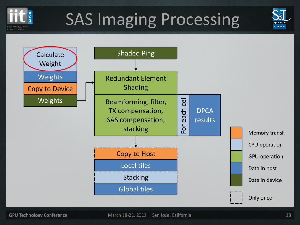
SAS Imaging Processing
Calculate Weight
Weights
Copy to Device
Weights
Shaded Ping
Redundant Element Shading
Beamforming, filter, TX compensation,
SAS compensation, stacking
Copy to Host
Local tiles
Stacking
Global tiles
CPU operation
GPU operation
Data in host
Data in device
Only once
Memory transf. For
each
cel
l
DPCA results
GPU Technology Conference March 18-21, 2013 | San Jose, California 38
SAS Imaging Processing
Calculate Weight
Weights
Copy to Device
Weights
Shaded Ping
Redundant Element Shading
Beamforming, filter, TX compensation,
SAS compensation, stacking
Copy to Host
Local tiles
Stacking
Global tiles
CPU operation
GPU operation
Data in host
Data in device
Only once
Memory transf. For
each
cel
l
DPCA results

GPU Technology Conference March 18-21, 2013 | San Jose, California 39
• Correct redundancy of the elements
• It depends on surge
• Example: 8 elements and displacement of 3
Redundant Element Shading
3 3 2 3 3 2 3 3 Ping n
Ping n+1
Ping n-1
...
...
...
...
0.333 0.333 0.5 0.333 0.333 0.5 0.333 0.333

GPU Technology Conference March 18-21, 2013 | San Jose, California 40
SAS Imaging Processing
Calculate Weight
Weights
Copy to Device
Weights
Shaded Ping
Redundant Element Shading
Beamforming, filter, TX compensation,
SAS compensation, stacking
Copy to Host
Local tiles
Stacking
Global tiles
CPU operation
GPU operation
Data in host
Data in device
Only once
Memory transf. For
each
cel
l
DPCA results

GPU Technology Conference March 18-21, 2013 | San Jose, California 41
• Multiply the acoustic data by the weight:
Where:
– 𝐴𝑗𝑤 is the weighted acoustic data of the element 𝑗
– 𝐴𝑗 is the acoustic data of the element 𝑗
– 𝑤𝑗 is the weight for the element 𝑗
• The multiplication is done in place (acoustic data is overwritten), to save memory.
Redundant Element Shading
𝐴𝑗𝑤 = 𝐴𝑗 ∙ 𝑤𝑗

GPU Technology Conference March 18-21, 2013 | San Jose, California 42
SAS Imaging Processing
Calculate Weight
Weights
Copy to Device
Weights
Shaded Ping
Redundant Element Shading
Beamforming, filter, TX compensation,
SAS compensation, stacking
Copy to Host
Local tiles
Stacking
Global tiles
CPU operation
GPU operation
Data in host
Data in device
Only once
Memory transf. For
each
cel
l
DPCA results

GPU Technology Conference March 18-21, 2013 | San Jose, California 43
• Each cell has:
– Min range
– Max range
• We calculate:
– Min X
– Max X
• With this values we have the bounding box (dark areas)
SAS Imaging - Beamforming
Range
X
GPU Technology Conference March 18-21, 2013 | San Jose, California 44
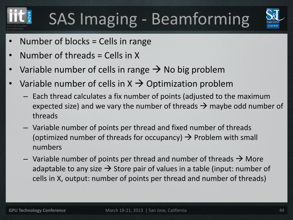
• Number of blocks = Cells in range
• Number of threads = Cells in X
• Variable number of cells in range No big problem
• Variable number of cells in X Optimization problem – Each thread calculates a fix number of points (adjusted to the maximum
expected size) and we vary the number of threads maybe odd number of threads
– Variable number of points per thread and fixed number of threads (optimized number of threads for occupancy) Problem with small numbers
– Variable number of points per thread and number of threads More adaptable to any size Store pair of values in a table (input: number of cells in X, output: number of points per thread and number of threads)
SAS Imaging - Beamforming

GPU Technology Conference March 18-21, 2013 | San Jose, California 45
• Blocks and threads distribution
SAS Imaging - Beamforming
1 2 3 4
1 2 3 4 1 2
1 2 3 4 1 2
1 2 3 4 1 2
1 2 3 4 1 2 3 4
1 2 3 4 1 2 3 4
1 2 3 4 1 2 3 4
1 2 3 4 1 2 3 4 1 2
1 2 3 4 1 2 3 4 1 2
1 2 3 4 1 2 3 4 1 2
Blocks (range)
Threads (X)

GPU Technology Conference March 18-21, 2013 | San Jose, California 46
• Range index (r) and position (R) of the block:
where: – 𝑟𝑚𝑖𝑛 and 𝑟𝑚𝑎𝑥 are the minimum and maximum range index
– 𝑅𝑚𝑖𝑛 and 𝑅𝑚𝑎𝑥 are the minimum and maximum range distance
– 𝑁𝑏 is the number of blocks
– 𝑟 is the range index
– 𝑅 is the range distance
– 𝑅𝑟𝑒𝑠 is the resolution
SAS Imaging - Beamforming
𝑟 = 𝑟𝑚𝑖𝑛 + 𝑗,where 𝑗 = 0. . 𝑁𝑏 − 1 and 𝑁𝑏 = 𝑟𝑚𝑎𝑥-𝑟𝑚𝑖𝑛
𝑅 = 𝑟 ∙ 𝑅𝑟𝑒𝑠 + 𝑅𝑚𝑖𝑛

GPU Technology Conference March 18-21, 2013 | San Jose, California 47
• Calculate 𝑥𝑚𝑖𝑛 and 𝑥𝑚𝑎𝑥 from range and beam angle
• X index of the thread:
Alternative calculation (slower): 𝑥 = 𝑥𝑚𝑖𝑛 + 𝑖 ∙ 𝑁𝑝𝑡 + 𝑘
where:
– 𝑥𝑚𝑖𝑛 and 𝑥𝑚𝑎𝑥 are the minimum and maximum X index
– 𝑁𝑡 is the number of threads
– 𝑁𝑝𝑡 is the number of points per thread
– 𝑥 is the X index
• Conversion between index and position analogue to range, with 𝑋, 𝑋𝑚𝑖𝑛, 𝑋𝑚𝑎𝑥 and 𝑋𝑟𝑒𝑠
SAS Imaging - Beamforming
𝑥 = 𝑥𝑚𝑖𝑛 + 𝑖 + 𝑘 ∙ 𝑁𝑡 , where 𝑖 = 0. . . 𝑁𝑡 − 1 and 𝑘 = 0. . . 𝑁𝑝𝑡 − 1
GPU Technology Conference March 18-21, 2013 | San Jose, California 48
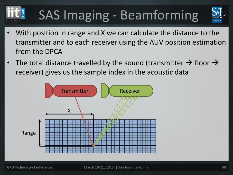
• With position in range and X we can calculate the distance to the transmitter and to each receiver using the AUV position estimation from the DPCA
• The total distance travelled by the sound (transmitter floor receiver) gives us the sample index in the acoustic data
SAS Imaging - Beamforming
Range
X
Transmitter Receiver

GPU Technology Conference March 18-21, 2013 | San Jose, California 49
• Instead of taking one single sample, we use a filter similar to sinc
• Store acoustic data and filter in 1D textures (float2 format)
SAS Imaging - Filter
distanceTransmitter = calculate_distance_to_transmitter(posTransmitter, posTile)
tileAcc = 0.0
for each receiver
distanceReceiver = calculate_distance_to_receiver(posReceiver, posTile)
pathLength = distanceTransmitter + distanceReceiver
indexData = calculate_index_data(pathLength)
indexFilter = calculate_index_filter(...)
tileSum = 0.0
for filter size
tileSum += filter(...) * acousticData(...)
next
tileAcc += tileSum * distanceReceiver
next
tileAcc *= distanceTransmitter / nReceivers

GPU Technology Conference March 18-21, 2013 | San Jose, California 50
• Multiply the accumulated value by the compensation factors:
– TX compensation: Eliminate rippling effects (similar to inverse sinc filter)
– SAS compensation: Add smoothing in the beam
• Stacking:
– Accumulate value in the tile
SAS Imaging - Compensation

GPU Technology Conference March 18-21, 2013 | San Jose, California 51
• Performance depends on the resolution and range
• Three configurations: A. Testing: Short range (110-150m), medium resolution (0.025x0.050), port side
B. Sea trials: Full range (35-145m), medium resolution (0.050x0.050), both sides
C. Scientific: Full range (35-145m), high resolution (0.025x0.015), port side
SAS Imaging - Results
CPU1 GPU2 Speedup
A 3663.8ms 47.8ms x77
B 8614.2ms 115.0ms x75
C 28588.2ms 352.9ms x81
1 Running on an Intel Core i7-920 @ 2.67 GHz 2 Running on a NVIDIA Tesla C1060

GPU Technology Conference March 18-21, 2013 | San Jose, California 52
Global performance
CPU1 GPU2 Speedup
Pre-processing 84.3 ms 3.7 ms x23
DPCA 93.5 ms 18.4 ms x5
Imaging A 3663.8ms 47.8ms x77
Imaging B 8614.2ms 115.0ms x75
Imaging C 28588.2ms 352.9ms x81
Pings per second A 0.26 14.3 x55
Pings per second B 0.11 6.3 x57
Pings per second C 0.035 2.7 x77
1 Running on an Intel Core i7-920 @ 2.67 GHz 2 Running on a NVIDIA Tesla C1060

GPU Technology Conference March 18-21, 2013 | San Jose, California 53
• Software tested on board an AUV
• x86 processor with a NVIDIA GT240 equivalent graphics card
• 4 pings per second (250ms between pings)
• Running in real-time in medium resolution (configuration B)
Sea Trials

GPU Technology Conference March 18-21, 2013 | San Jose, California 54
• Upgrade the on-board GPU to calculate in real-time in high resolution
• Further software improvements to increase performance
• Continue development of multi-GPU and multi-CPU versions for desktop computers (scientific research)
• Add further algorithms in the chain (interferometry generate 3D images from bathymetric and main arrays)
• Update algorithms? Adapt them to GPU
• Currently testing the NVIDIA Carma platform It’s already running!
Future work
GPU Technology Conference March 18-21, 2013 | San Jose, California 55
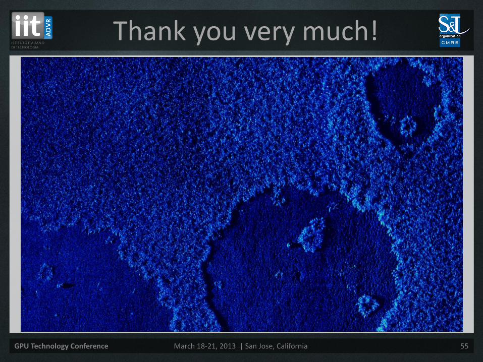
Thank you very much!