Embed Size (px)
Citation preview

Government Spending and Economic Recovery: A State Comparison during the Great Recession
MPP Professional Paper
In Partial Fulfillment of the Master of Public Policy Degree Requirements The Hubert H. Humphrey School of Public Affairs
The University of Minnesota
Conrad Segal
May 12, 2014 Signature below of Paper Supervisor certifies successful completion of oral presentation and completion of final written version: ________________________ ____May 7, 2014___ May 12, 2014 ___________ Morris Kleiner, Professor Date, oral presentation Date, paper completion ________________________ May 12, 2014_________________ Thomas Stinson, Professor Date
1

Executive Summary
In late 2007, the U.S. entered the worst recession since the Great Depression. State
and local governments saw large decreases in their revenues and, due to their
constitutions, were forced to balance their budgets, usually by reducing spending.
The loss in state and local government spending during the recession was countered
by two large federal expenditures totaling over a trillion dollars. Every state had a
different amount of per capita government spending during the recession. This
paper aims to answer the question: did states that, relative to other states, had high
amounts of per capita government spending recover faster economically than states
with low amounts of per capita government spending? Using national macro data,
much of which comes from the census and the Bureau of Economic Analysis, and
OLS models, I conclude that states that had high amounts of government spending,
either in their capital or current budgets, recovered 5% faster in both GSP and
payroll. The data also suggest that the full effect of the stimulus spending was over
by 2011.
Introduction
“It’s the economy stupid.”
-James Carville
A 2013 poll by CBS News asked voters what they thought was the most important
issue facing the United States today. The largest percentage, 31%, said the economy
or jobs.i Almost every poll over the last decade has shown similar results with the
economy rarely rating below 30% and frequently polling in the 40’s. However,
there exists a great debate amongst policy makers, politicians, and economists on
how best to stimulate a sluggish economy. On one side are Keynesian economists
who believe in government spending as a way to provide economic stimulus.
Democrats in the federal government also tend to believe in this theory. On the
2

other side are classical economists who believe in minimal government intervention
with subsequent low tax rates. Republicans generally support this approach.
In late December 2007, the United States faced the worst economic recession since
the Great Depression. The recession was felt worldwide and included: decreases in
housing values, limited credit, GDP loss, and an increase in unemployment.
Different agencies in the U.S. responded differently to the recession, some with
polices never seen before. The Fed, for example, responded by cutting interest rates
to a record near zero.ii
Given the political tendencies of the two parties, one would expect conservative
states to take a laissez-faire approach to the recession, while liberal states to be
hands on and pass stimulus bills. However, most state and local governments are
required by law to maintain balanced budgets. A 2008 National Conference of State
Legislatures Report states that 43 states are constitutionally required to keep
balanced budgets.iii According to the Quarterly Summary of State & Local Tax
Revenue put out by the U.S. Census, in 2012 state and local governments received
24% of their revenue from income tax, 33% from property tax, and 21% from sales
tax.iv When the recession hit, 8 million Americans lost their jobs, which meant less
revenue from income taxes.v Less income and low consumer confidence also meant
fewer purchases and therefore less sales tax revenue. According to Zillow, the total
U.S. housing market fell by $6.3 trillion from 2007-2011.vi This, coupled with a
record amount of foreclosures, greatly reduced property tax revenue. The result of
large losses in revenue for state and local governments combined with legal
requirements to keep balanced budgets meant that many state and local
governments had to make dramatic reductions to their budgets. Figure 1 shows
how, in 2008, state and local government spending contributed almost nothing to
the national GDP.
3

Figure 1: State, Local, and Federal Government Contributions to GDPvii
Partisan division was apparent at the federal level where two stimulus packages
were passed totaling $1,531 billion in government spending. The Emergency
Economic Stabilization Act of 2008 spent $700 billion on distressed assets, with an
emphasis on subprime mortgages as well as supplying banks with cash.viii The
following February, the federal government passed the American Recovery and
Reinvestment Act of 2009 (ARRA). The ARRA cost $831 billion and its aim was “job
preservation and creation, infrastructure investment, energy efficiency and science,
assistance to the unemployed, and State and local fiscal stabilization”.ix, The ARRA
was supported by a democratic president and a democratic majority in the House
and Senate. Only three Republicans (one of whom soon switched parties) in the
House and Senate voted for the bill.x Liberal economists such as Paul Krugman and
Joseph Stiglitz supported a large stimulus while conservative economists such as
4

Edward Prescott and Gary Becker opposed the ARRA. The theories and data behind
this disagreement will be further discussed in the next section of this paper.
It is impossible to know if the ARRA was a good policy response to the Great
Recession. Unlike physical scientists, economists cannot rerun the experiment with
different polices. It’s possible that a larger stimulus would have led to a faster
recovery or it’s possible that the stimulus slowed down the recovery; one can never
know with certainty. In other words, it is impossible to know the counter factual.
However, this paper tries to answer this question by comparing the amount of
government money different states spent during the recession. No two states are
the same and the Great Recession affected each state differently; this paper aims to
control for these differences. The models in this paper use per capita government
spending to see if states that had more per capita government spending recovered
their GSP and/or employment faster than those with less per capita government
spending. Answering this question will help policy makers decide what course of
action to take the next time a recession occurs.
Literature Review
Economics Theories
The dependent variable for this paper is economic recovery time. There are
different metrics one could use to determine economic recovery time; this paper
uses gross state product (GSP) as one of the determinants. There are different ways
to define GDP. This paper defines GDP as consumption plus investment plus
government spending plus trade balance (GDP=C+I+G+XM). Using this formula, one
would predict higher government spending would lead to higher GDP.
There are different schools of economic thought. Today, the two most popular
schools are Keynesian, sometimes called neo-Keynesian or New Keynesian, and free
market, sometimes called the Austrian School or neoclassical. Keynesian economics
relies on the Investment Saving-Liquidity Preference Money Supply (IS-LM) model.
5

In the short-run Keynesians believe that aggregate demand can grow by either
expansionary monetary policy or expansionary fiscal policy. Expansionary
monetary policy in the U.S. must be carried out by the Federal Reserve (FED) and is
done by purchasing securities, lowering the federal discount rate, or lowering the
reserve requirement for banks. The result of all three of these changes is to increase
the money supply, which shifts the LM curve downward, which raises income, which
increases aggregate demand (shown in Figure 2). Increasing government spending
or cutting taxes are ways to expand fiscal policy, which shifts the IS curve to the
right, which increases income, which increases aggregate demand (shown in Figure
3). The important takeaway is that Keynesian theory supports the idea that higher
per capita government spending will help state economies more than lower per
capita government spending.
Figure 2xi: Expansionary monetary policy
6
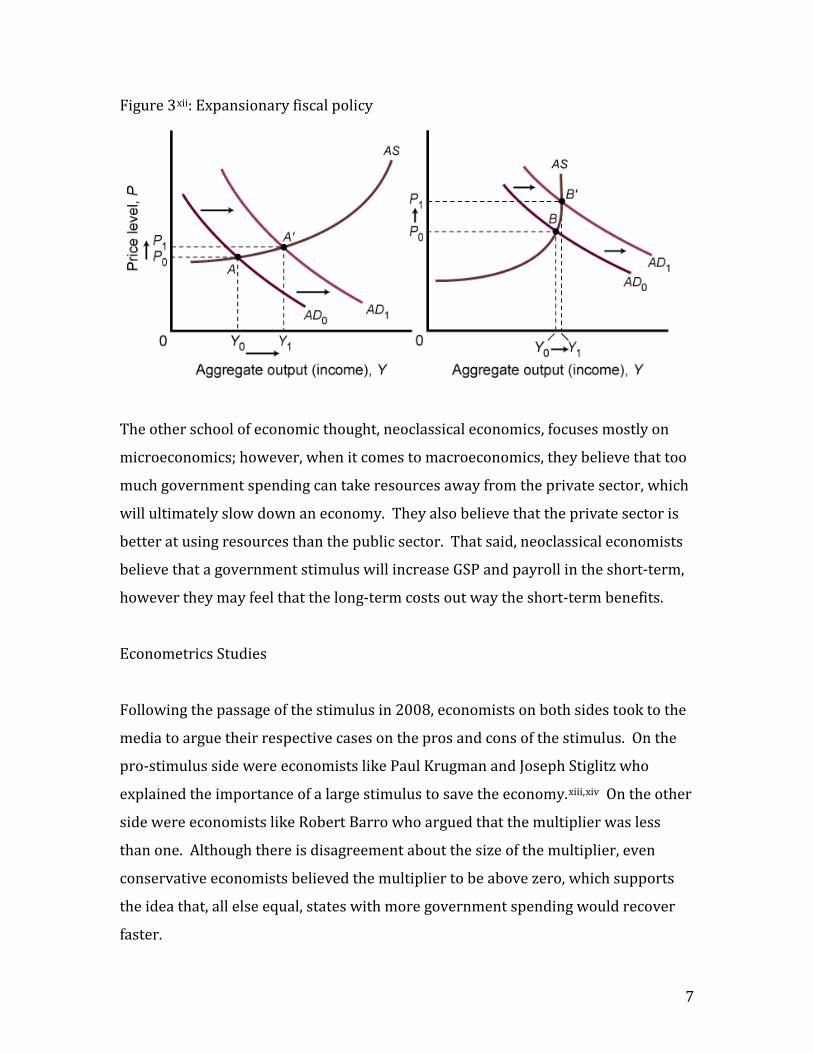
Figure 3xii: Expansionary fiscal policy
The other school of economic thought, neoclassical economics, focuses mostly on
microeconomics; however, when it comes to macroeconomics, they believe that too
much government spending can take resources away from the private sector, which
will ultimately slow down an economy. They also believe that the private sector is
better at using resources than the public sector. That said, neoclassical economists
believe that a government stimulus will increase GSP and payroll in the short-term,
however they may feel that the long-term costs out way the short-term benefits.
Econometrics Studies
Following the passage of the stimulus in 2008, economists on both sides took to the
media to argue their respective cases on the pros and cons of the stimulus. On the
pro-stimulus side were economists like Paul Krugman and Joseph Stiglitz who
explained the importance of a large stimulus to save the economy.xiii,xiv On the other
side were economists like Robert Barro who argued that the multiplier was less
than one. Although there is disagreement about the size of the multiplier, even
conservative economists believed the multiplier to be above zero, which supports
the idea that, all else equal, states with more government spending would recover
faster.
7

Now that the recession is over, some economists have tried to figure out how big the
multiplier was. Ilzetski, Mendoza, and Vegh came up with a model that looked at the
multiplier from 44 different countries. Between the 44 countries, the multiplier
ranged from .5 to 1.5.xv Again, all the multipliers are above zero, which means that
my study should show positive coefficients on the high spending states.
Data & Variable Explanation
The goal of this paper is to see if government spending leads to faster economic
recovery. There are different ways to define government spending. The all-
encompassing measure is total expenditure, which is the total amount of federal,
state, and local government money spent in a given fiscal year. This metric was not
used, since roughly a quarter of state’s expenditures are intergovernmental
expenditures, meaning that they go to other levels of the government.xvi Subtracting
intergovernmental expenditures from total expenditures leaves direct expenditures.
Direct expenditures are divided into five parts: xvii
• Current operation: “Direct expenditure for compensation of own officers and
employees and for supplies, materials, and contractual services except any
amounts for capital outlay.”
• Capital outlay: “Direct expenditure for purchase or construction, by contract
or government employee, construction of buildings and other improvements;
for purchase of land, equipment, and existing structures; and for payments
on capital leases.”
• Insurance benefits and repayments: “Social insurance payments to
beneficiaries, employee-retirement annuities and other benefits, and
withdrawals of insurance or employee retirement contributions.”
8

• Assistance and subsidies: “Cash contributions and subsidies to persons, not
in payments for goods or services or claims against the government. For
states, it also includes veterans' bonuses and direct cash grants for tuition,
scholarships, and aid to nonpublic education institutions.”
• Interest on debt: “Interest on debt is the amount of money paid by the state
for monies borrowed.”
Of these five I chose to use current operation and capital outlay as the independent
variables. Current operation makes up approximately two thirds of the entire state
budget and includes government employee salaries and almost all government
services. Capital outlays were also used since it includes construction costs, which
were a large percentage of the ARRA. The remaining three categories were not used
since they are not areas that were greatly affected by the recession, the ARRA, or
had a large effect on state economic recoveries. The census gathers all this data
from the states in their State Government Finance section.xviii
Economic recovery is another term that can be defined with different metrics. Stock
market, unemployment percentage, Gross Domestic Product (GDP), inflation
percent, and poverty rate are all ways economists analyze a region’s economy. For
this paper I chose to use Gross State Product (GSP) and payroll. Unemployment
reached 10% in October of 2009, which is the highest rate in the U.S. since 1983.xix
Due to the severity of unemployment, the media attention that was given to
unemployment, and the ARRA goal of reducing unemployment, including
unemployment was necessary. Unemployment is the percentage of people actively
looking for work. It therefore does not include underemployed people, people in
jobs that pay less than their previous job, and people who have given up looking for
a job and dropped out of the job market. Studies have shown that all three of these
phenomena happened in large numbers as a result of the Great Recession.xx One
9

way to avoid these issues is to use U6 unemployment data, which includes
"marginally attached workers and those working part-time for economic reasons.”
Unfortunately, U6 is not available at the state level so instead payroll was used.
Payroll data is from the Bureau of Labor Statistics Quarterly Census of Employment
and Wages surveyxxi and gives the amount of total wages in a state for a given year.
Using this metric accounted for the unemployed, those in lower paying jobs, and
people who dropped out of the workforce.
GSP was also used to evaluate the recovery of a state’s economy. GSP was chosen
since it does the best job of covering the entire economy of a given state. GSP should
measure the strength of a state’s economy and payroll should define the strength of
the state’s labor market. GSP data is in the same place as capital outlays and current
operations in the censusxxii.
Every state economy is different and therefore the Great Recession affected every
state differently. In order to accurately see if high per capita government spending
states recovered better than low spending states, one must control for these
differences. To accomplish this, nine covariates were included in the regressions.
Recessions can cause displacement of people. Home forecloses and job loss may
force people to move. Some people in states that were hit hardest by the recession
moved to states that were hit less hard. In order to control for this difference,
change in population, a variable that compares the change in population from the
current year to the previous year, was added.
Impoverished residents cost the government money through programs like
Medicaid, food stamps, EITC, unemployment, and Welfare. States have different
numbers of residents below the poverty line and the recession changed the
percentage in every state differently. Data from the Census Bureau’s Housing and
Household Economic Statistics Division was used to control for this difference.xxiii
10

The percentage of poor people in a state is not the only way to sense its income
distribution. A state’s median income was also used as a covariant. It was included
to control for any differences low and high-income level states might have in dealing
with the recession differently. Median income data is from the census.xxiv
Every state runs its own Medicaid program. Every state’s program is also partially
funded by the federal government. One way the federal government gave states
financial relief during the recession was to increase the percentage of state’s
Medicaid that was paid for by the federal government. Of the $831 billion 2009
federal stimulus package, $87 billion went to increase state’s Medicaid.xxv This freed
up money in states’ budgets that no longer had to go towards Medicaid, but instead
could go to economic stimulus. Since every state runs their Medicaid program
differently, they received different per capita amounts and this needed to be
controlled. Data for the number of state residents on Medicaid and the percentage
the federal government paid in that state is from the Kaiser Foundation.xxvi Taking
the number of residents on Medicaid multiplied by the federal percentage results in
the total amount of federal money spent in a given state on Medicaid.
Certain industries were hit harder during the recession than others. Industries in
the financial sector and construction were hit especially hard. Some states have
work forces with a higher percentage of recession-hit industries, so it was important
to control for these differences. I included the five largest industries to control for
these differences: construction, manufacturing, retail, finance and education. Not
only do these five industries have the largest wages, but they also experienced the
five largest job losses during the recession.xxvii
xxviii
Data for the industries is from the
Current Population Survey (CPS).
11

Methodology
When deciding which methodology to use to test the hypothesis that states that had
higher per capita government spending during the recession recovered faster than
those that had lower per capita spending, a few decisions needed to be made. The
first issue was how to deal with time periods. The data gathered was from 2005-
2012 and the official recession, according to the National Bureau of Economic
Research, started in December 2007 and ended in June 2009.xxix Figures 4 and 5
show the national trend for the two dependent variables, GDP and unemployment.
Non-recession GDP appears to stop somewhere between 2006 and 2007, bottoms
out at the end of 2009, and doesn’t recover until 2011. Non-recession
unemployment also appears to stop somewhere between 2006 and 2007, bottoms
out at the end of 2009, but as of the end of 2012 still had not recovered to pre-
recession levels. Given the national trends, 2005 was used as the state’s pre-
recession level, 2009 was the peak of the recession or trough, and since GDP and
unemployment recovered at different times, both 2011 and 2012 were used to
determine economic recovery. For government spending during the recession
period, 2008 through 2010 was used.
Figure 4xxx GDP Annual Growth Rate
12

Figure 5xxxi Unemployment Rate
The next issue that needed to be addressed was whether economic recovery should
be measured from the base year or the trough. Depending on which metric was
used, the results could be very different. For example, states A and B have a pre-
recession GSP of 10 and 20 respectively. During the recession, state A’s GSP falls to
5 while state B’s falls to 8. At the end of 2012, State A has recovered back to 9 while
State B has recovered to 17.
Table 1 Economic recovery Trough vs. Prerecession
State A State B
Pre 10 20
Trough 5 8
Post 9 17
Post/Pre .9 .85
Post/Trough 1.8 2.125
Comparing pre-recession to post-recession, state A recovered faster (.9>.85);
however, if one compares the trough to post-recession, state B recovered faster
(2.125>1.8). To deal with these potential differences, regressions were run using
both time periods.
13

Another issue that needed to be addressed was how to deal with the independent
variables, capital and current government spending. Just looking at state
government per capita spending during the recession might not be an adequate
measure of state government spending relative to other states. Alaska had the
highest per capita government spending during the recession, but it also had the
highest pre-recession per capita spending. It was possible for a high spending state
during the recession to have actually spent less per capita proportional to other
states. A fictional example is shown in Table 2. State A had the highest per capita
spending during the recession (8 compared to 6 and 5), but of the three states it is
the only one that decreased its per capita spending relative to before recession
spending.
Table 2 Average spending vs. Average spending/base year spending
State Pre Recession per
Capita Spending
During Recession Per
Capita Spending
Recession Spending/
Pre Recession Spending
A 10 (1) 8 (1) .8 (3)
B 5 (2) 5 (3) 1 (2)
C 4 (3) 6 (2) 1.5 (1)
To deal with this issue, both per capita government spending during the recession
and change in government spending were analyzed.
Change in government spending = 2008 through 2010 per capita spending/ 2005
per capita spending.
The last issue that had to be addressed was how to deal with 50 states. Creating a
dummy for all 50 states would not be a good method for many statistical reasons,
including loss of degrees of freedom and high standard errors. Instead, three groups
were created. For each regression, the states were ranked highest to lowest in per
capita government spending; the highest 16 states were marked as high, the middle
14

18 as medium and the lowest 16 as low. Comparing the coefficient on high spending
states to low spending states should show the biggest difference, if a difference
exists.
It should also be noted that every variable that was not a percent or median was
changed to per capita in order to eliminate the differences in state populations.
Thirty-two separate ordinary least squared models (OLS) were run. There are 32
different regressions due to 5 variations:
• Independent variable variations
o Capital vs. current budget spending
o 2008-2010 per capita spending vs. 2008-2010 per capita spending /
2005 per capita spending
• Dependent variable variation
o GSP vs. payroll
o 2011 vs. 2012 as the recovery year
o Comparing recovery from pre recession vs. recovery from trough
Each of the 32 regressions used the same covariates, which are listed below: The
data section describes why these covariates were selected.
Population change: high year population/ low year population (PopC)
State poverty rate: average percentage over the time period (PR)
Federal Medicaid payments: average per capita dollar amount over the time
period (MP)
Median income: average over the time period (MI)
Construction wages: average per capita over the time period (CW)
Manufacturing wages: average per capita over the time period (MW)
Retail wages: average per capita over the time period (RW)
15

Finance wages: average per capita over the time period (FW)
Education wages: average per capita over the time period (EW)
Depending on which independent and dependent variable was used in the
regression, that particular regression may have covered a different time period than
other regressions. In fact, the 32 regressions covered four different time periods, all
ranging somewhere between 2005-2012. Covariates were only used from the
regression’s time period. For example, a regression that went from 2008-2011 only
used average construction wages from 2008-2011, as opposed to a regression that
went from 2005-2011, which used average construction wages from 2005-2011.
The basic function for all 32 of these regressions is the following:
EconomicRecovery = C1HighSt + C2 MediumSt + C3PopC + C4PR +C5MP +C6MI
+C7CW + C8MW + C9RW + C10FW + C11EW +cons
• Economic Recovery is a combination of GSP/Payroll, 2011/2012, and
trough/base
• HighSt is a dummy for the 16 highest states in a combination of
capital/current budget and average spending or average spending /base year
spending
• MediumSt is a dummy for the 18 middle states in a combination of
capital/current budget and average spending or average spending /base year
spending
• Cons is the constant
Assumptions for the Model
1. This paper assumed that all government spending from the stimulus
had an equal effect on GSP and payroll. Some stimulus money may have had
16

a larger effect or a faster, more direct effect than other stimulus money;
however, it was assumed that it all had the same effect.
2. There are four ways for an economy’s GDP to grow. In this paper it
was assumed that private consumption and investment were affected
similarly in each state. In order words, it was assumed that residents in one
state changed their consumption and investment habits as a result of the
recession in a similar manner to residents in other states.
3. Covariates included in the regression dealt with any potential omitted
or selection bias.
Results
Meta-Analysis
Table 3 Aggregated Results for 32 Models (Coefficient)
Mean
Coefficient
Median
Coefficient
Difference from
Mean
All 32 0.04995 0.03798 -
Current 0.05118 0.04517 -0.00123
Capital 0.04871 0.03798 0.00123
Average Spending 0.05698 0.06196 -0.00703
Average/Base 0.04292 0.03635 0.00703
2011 0.04933 0.03798 0.00061
2012 0.05056 0.04564 -0.00061
Payroll 0.04970 0.03635 0.00025
GSP 0.05019 0.04145 -0.00025
Trough 0.01468 0.01573 0.03526
Base 0.08521 0.08818 -0.03526
17

Table 4 Aggregated Results for 32 Models (p-values)
Mean p-value Median p-value
Difference from
Mean
All 32 0.21991 0.08900 -
Current 0.28925 0.06400 -0.06934
Capital 0.15056 0.10150 0.06934
Average Spending 0.29075 0.03550 -0.07084
Average/Base 0.14906 0.09400 0.07084
2011 0.18556 0.05800 0.03434
2012 0.25425 0.11950 -0.03434
Payroll 0.20738 0.08400 0.01253
GSP 0.23244 0.08900 -0.01253
Trough 0.40200 0.29600 -0.18209
Base 0.03781 0.02200 0.18209
This section of the paper provides meta-analysis for all the regressions that were
run in this paper. Since there are 32 different results it is not practical (or
interesting) to discuss each result individually. Tables 3 and 4 give summary results
for the 32 OLS regressions (full results can be found in the appendix). Table 3 gives
the coefficient for the states that spent a high amount per capita (16 highest states)
relative to the low spending states (16 lowest states) and Table 4 gives the
corresponding p-values. The tables begin by giving the mean and median for the 32
regressions. As discussed in the methodology section, there are five variations that
create the 32 different models. Tables 3 and 4 break down each variation,
comparing the 16 models that used that method as opposed to the 16 that used the
other method. The last column notes the difference of the coefficient for that
particular group compared to the average coefficient for all 32 models.
The average coefficient for all 32 regressions is .05. This means that if all else is
equal, states that had relatively high per capita government money spent in them
during the recession recovered 5% more in GSP and payroll than states that had
relatively low per capita government money spent in them during the recession.
18

This finding suggests that government spending does in fact decrease the effects of a
recession. It should be noted that the average p-value for the 32 regressions is .22,
which is higher than one would like in order to claim strong results, however the
median p-value is much lower at .09, which is low enough to show significance. It
should be noted that these regressions contain only 50 observations, so that getting
very low p-values is not easy. It should also be noted that the p-value on the high
per capita government-spending coefficient is by far the lowest p-value of all the
covariates.
Current vs. Capital
There is only a .001 average difference between the current and capital coefficients.
This means that government money that went towards current expenditure items
stimulated the economy just as much as money that went toward capital
investments. One might have expected that money spent in the current budget
would have a faster stimulating effect, since money spent on capital projects would
take time to see returns to the economy, but that does not seem to be the case.
However, much of the capital money spent had immediate economic stimulus effects
such as construction worker wages, building materials, and construction contracts.
Average Spending (2008-2010) vs. Average/Base (2008-2010/2005)
Separating states using their per capita average government spending during the
recession resulted in a .014 higher mean coefficient and an even higher median
difference of .026 compared to sorting states by looking at change in government
spending comparing their base year to recession year spending. Going into the
study, I expected the reverse finding, since change in government spending seems to
be a more accurate way to look at government spending. One explanation for this
difference has to do with which states are included in the two groups. When one
looks at the high spending states using the per capita government spending model
during the recession, a lot of progressive northeastern states are included:
Connecticut, Delaware, New Jersey, Maine, New York, Rhode Island, and Vermont.
Contrast this to the high spending states in the change in government spending
19

model and one sees more conservative states: Alabama, Kansas, Oklahoma, Montana,
Tennessee, and Arizona. The difference in the coefficient might have to do with how
progressive northeastern states were able to cope with the recession compared to
conservative states.
2011 Recovery Year vs. 2012 Recovery Year
Using the mean coefficients from 2011 as compared to 2012 as the recovery year
yielded no statistical difference (.0009). One would need more years of data (2013,
2014, etc.) to draw conclusions using different recovery years. However, if
coefficients for 2013 and 2014, etc. also had no statistical difference, it might be the
case that government money spent during the recession had its full economic
stimulus effect already exhibited by 2011. Since most of the ARRA was designed for
immediate economic stimulus, it would mean that the ARRA did a good job of
accomplishing that part of its goal.
Payroll vs. GSP
Using payroll as opposed to GSP for the dependent variable yields almost no
difference. For both metrics, being a high spending state leads to a 5% increase in
payroll and GSP when compared to an identical low spending state. This is an
interesting finding, since GSP recovered faster than payroll. One might suspect that
the government spending effect would be higher for GSP than payroll, especially
when using 2011 as the recovery year, however this does not appear to be the case.
This finding, paired with the previous 2011 vs. 2012 finding, further suggests that
states that spent more during the recession saw the economic stimulus from this
higher spending right away and did not need to wait for results.
Trough vs. Base
Comparing the recovery to the base year vs. trough year yielded by far the largest
difference for the independent coefficient. Using the base year (2005) as the
comparison for the recovery had a very high .085 coefficient as opposed to using the
trough year (2009) which had a low .015 coefficient. The large difference in these
20

findings can be explained in Figure 6, which shows national per capita wages from
2005 through 2012. Comparing 2011 or 2012 to the base year reveals a large
increase in payroll, however when comparing 2011 or 2012 to the trough year,
there is a very small increase in wages. The base year coefficient is therefore much
higher, since it needs to account for a much larger payroll increase when compared
to the trough year.
Figure 6
Covariates
Table 5 Covariates
Covariates Positive Negative
Average p-
Value
Population Change 6 26 0.51453
Poverty Level 5 27 0.40744
Federal $ on Medicaid 14 18 0.60981
Median Income 0 32 0.30131
Construction Wages 25 7 0.47772
Manufacturing Wages 20 12 0.46178
Retail Wages 26 6 0.65884
Finance Wages 15 17 0.77866
Education Wages 11 21 0.78847
39.9
40
40.1
40.2
40.3
40.4
40.5
40.6
40.7
40.8
2005 2006 2007 2008 2009 2010 2011 2012
21

Looking at the results for the covariates, the only consistent finding is the
inconsistency in the covariates throughout the 32 regressions. Table 5 gives the
number of times each coefficient was positive and negative for the 32 regressions as
well as the average P-value. The only covariate that has consistency is the median
income, which is negative in all models and has a p-value of .301 (which is still
pretty high). All other covariates change signs a minimum of 5 times and have very
high p-values. Due to the change in coefficient signs and high p-values, it would be
unwise to draw conclusions on the effect of any of the covariates.
48 States
The two states with the highest per capita government money spent in them were
Alaska and Hawaii. From 2008 through 2010, Alaska had almost 3 times more per
capita current operations government spending than the average state in the
continental U.S and 4 times more in capital spending. Hawaii also had more than the
average continental state with twice per capita in current operations and 1.5 times
in capital budgets. Since these states’ spendings were significantly higher than the
other 48 states, the 32 regressions were also run with Alaska and Hawaii removed
from the dataset. After removing Alaska and Hawaii, there were 16 states in each
government spending group. Table 6 shows the aggregate results from the 32
regressions. There is no statistical difference in the 32 regression models using 48
states compared to 50 states. The mean coefficient for all 32 regressions is different
by only .002, while the median value is the same. Similarly, the mean p-value is
different by only .04, and the median p-value is the same. My hypothesis as to why
removing Alaska and Hawaii doesn’t change the results is twofold. First, half the
models use a percent change in government spending, so Alaska and Hawaii are not
outliers is those cases. Second, Alaska was one of the states that recovered the
fastest economically, which supports the claim that higher government spending
leads to faster recovery.
22

Table 6 Aggregated Results with 48 states
mean
C median C mean P median P
total 0.047 0.040 0.251 0.089
current 0.047 0.044 0.254 0.098
capital 0.046 0.040 0.249 0.082
average spending 0.051 0.052 0.260 0.068
average/base 0.043 0.040 0.243 0.098
2011 0.046 0.040 0.180 0.069
2012 0.048 0.044 0.323 0.132
payroll 0.045 0.040 0.287 0.082
gsp 0.049 0.042 0.215 0.093
trough 0.015 0.014 0.457 0.374
base 0.079 0.080 0.046 0.038
Finding the Best Model
The problem with meta-analysis is that it doesn’t allow for meaningful
interpretation or a strong predictive model. This section attempts to deal with these
issues by determining a best model for both dependent variables: GSP and payroll.
Of the 32 regressions, 13 of them have p-values below .05 (interestingly, the average
coefficient on the large state dummy for these 13 regressions is almost double that
of the average 32 regressions). Interestingly, the two models with the lowest p-
values were identical in four of the five differences. They both used capital spending,
average spending during the recession, 2011 as the base year, and compared the
recovery to the base year. The only difference was one used GSP and the other used
payroll. Results for these two models are shown in Tables 7 and 8.
23

Table 7 Payroll Best Model
Coef. p-Value Coef. p-Value Coef. p-Value Coef. p-Value
Large 0.096 0.001 0.101 0.001 0.099 0.000 0.088 0.000
Medium 0.039 0.163 0.039 0.152 0.038 0.136 0.046 0.049
Pc -0.711 0.079 -0.686 0.086 -0.669 0.076
Pv -0.005 0.517
Md -0.354 0.720 -0.136 0.883
Mi -0.032 0.441 -0.014 0.648 -0.011 0.628
C -0.011 0.811 -0.005 0.917 -0.002 0.959
M -0.001 0.938 0.003 0.808 0.003 0.773
R 0.054 0.461 0.065 0.368 0.060 0.349
F -0.004 0.705 -0.005 0.648 -0.005 0.660
E -0.013 0.826 -0.015 0.801 -0.014 0.802
Cons 2.094 0.002 1.852 0.001 1.809 0.000 1.152 0.000
Obs 50 50 50 50
Adj. R^2 0.166 0.178 0.198 0.200
R^2 0.353 0.346 0.346 0.233
24
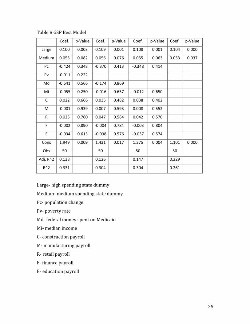
Table 8 GSP Best Model
Coef. p-Value Coef. p-Value Coef. p-Value Coef. p-Value
Large 0.100 0.003 0.109 0.001 0.108 0.001 0.104 0.000
Medium 0.055 0.082 0.056 0.076 0.055 0.063 0.053 0.037
Pc -0.424 0.348 -0.370 0.413 -0.348 0.414
Pv -0.011 0.222
Md -0.641 0.566 -0.174 0.869
Mi -0.055 0.250 -0.016 0.657 -0.012 0.650
C 0.022 0.666 0.035 0.482 0.038 0.402
M -0.001 0.939 0.007 0.593 0.008 0.552
R 0.025 0.760 0.047 0.564 0.042 0.570
F -0.002 0.890 -0.004 0.784 -0.003 0.804
E -0.034 0.613 -0.038 0.576 -0.037 0.574
Cons 1.949 0.009 1.431 0.017 1.375 0.004 1.101 0.000
Obs 50 50 50 50
Adj. R^2 0.138 0.126 0.147 0.229
R^2 0.331 0.304 0.304 0.261
Large- high spending state dummy
Medium- medium spending state dummy
Pc- population change
Pv- poverty rate
Md- federal money spent on Medicaid
Mi- median income
C- construction payroll
M- manufacturing payroll
R- retail payroll
F- finance payroll
E- education payroll
25

Columns 1 and 2 in Tables 7 and 8 give the coefficients and p-values for all variables
using the full models. The coefficient on the large state dummy is about .1 for both
models and has very low p-values of .001 and .003, respectively. This means, all else
equal, a state with high government spending during the recession would recover
10 % more in both payroll and GSP than an identical state with low government
spending during the recession. Another important take away is that none of the
other covariates have p-values anywhere low enough to signal significance.
When coming up with a list of covariates, I thought of all variables that could be
relevant in controlling for economic recovery. This does not mean that all of the
covariates should be included in the final models. Table 9 shows a correlation
matrix between all the covariates. The only variable that had the same sign on its
coefficients in all 32 models was median income. Since median income was the only
coefficient to have the same sign in all the models, it will be kept. Looking at the
correlation matrix, one sees that poverty rate is highly correlated with median
income. Intuitively this makes sense; states where people earn more will probably
have fewer poor residents. Given the high correlation, poverty rate was taken out of
the model and the results are shown in Columns 3 and 4 of Tables 7 and 8. The new
models have slightly higher coefficients on the large state dummy as well as slightly
lower p-values. The R2 not surprisingly goes down in both models, however the
adjusted R2 goes up in one model and falls slightly in the other.
26
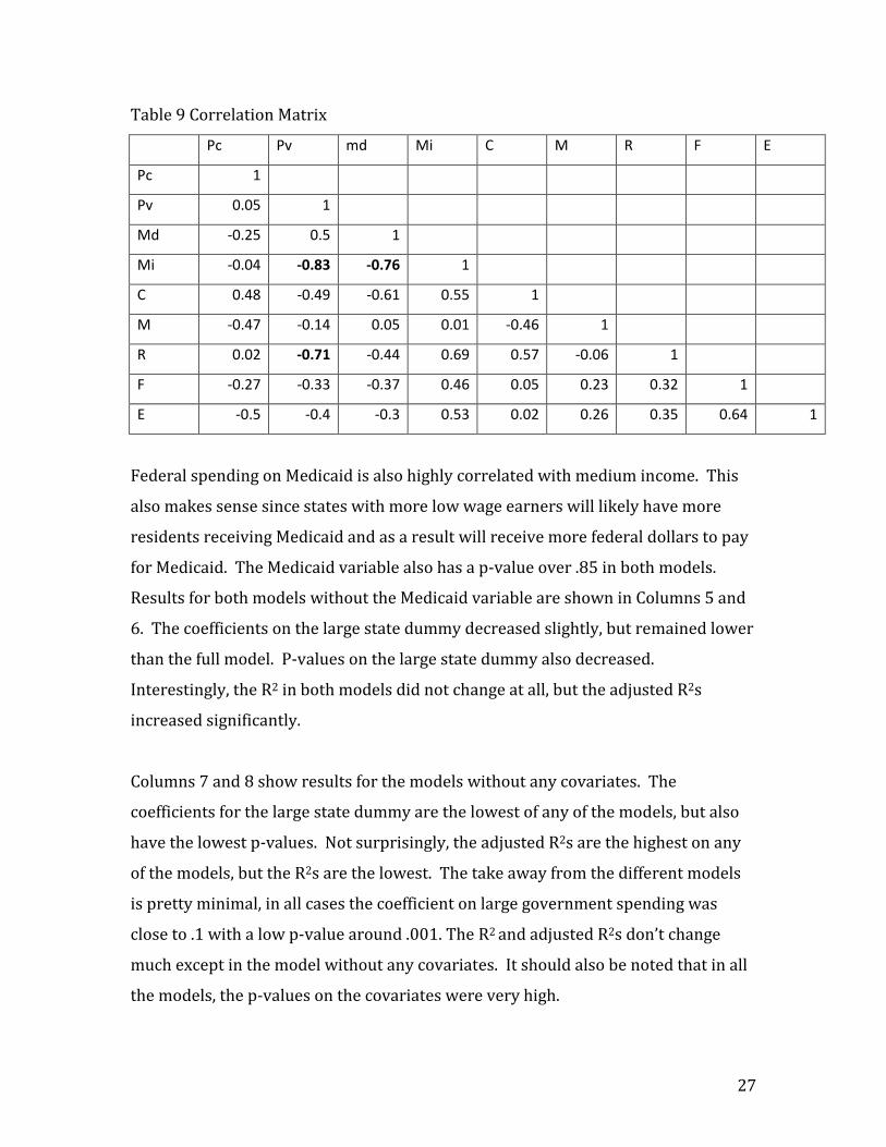
Table 9 Correlation Matrix
Pc Pv md Mi C M R F E
Pc 1
Pv 0.05 1
Md -0.25 0.5 1
Mi -0.04 -0.83 -0.76 1
C 0.48 -0.49 -0.61 0.55 1
M -0.47 -0.14 0.05 0.01 -0.46 1
R 0.02 -0.71 -0.44 0.69 0.57 -0.06 1
F -0.27 -0.33 -0.37 0.46 0.05 0.23 0.32 1
E -0.5 -0.4 -0.3 0.53 0.02 0.26 0.35 0.64 1
Federal spending on Medicaid is also highly correlated with medium income. This
also makes sense since states with more low wage earners will likely have more
residents receiving Medicaid and as a result will receive more federal dollars to pay
for Medicaid. The Medicaid variable also has a p-value over .85 in both models.
Results for both models without the Medicaid variable are shown in Columns 5 and
6. The coefficients on the large state dummy decreased slightly, but remained lower
than the full model. P-values on the large state dummy also decreased.
Interestingly, the R2 in both models did not change at all, but the adjusted R2s
increased significantly.
Columns 7 and 8 show results for the models without any covariates. The
coefficients for the large state dummy are the lowest of any of the models, but also
have the lowest p-values. Not surprisingly, the adjusted R2s are the highest on any
of the models, but the R2s are the lowest. The take away from the different models
is pretty minimal, in all cases the coefficient on large government spending was
close to .1 with a low p-value around .001. The R2 and adjusted R2s don’t change
much except in the model without any covariates. It should also be noted that in all
the models, the p-values on the covariates were very high.
27
Conclusion
There may never be political or academic agreement on stimulus spending during a
recession. This paper does not attempt to decipher what would have happened to
the economy with no stimulus, a smaller stimulus, a larger stimulus, or estimate the
multiplier for stimulus spending. This paper does however, by looking at
government spending in states during the recession, support the economic theory
that government spending in a recession does in fact increase payroll and GSP.
Using 32 OLS models with two variations on the independent variable and three
variations on the dependent variable, I found that states with high amounts of
government spending recovered 5% more in GSP and payroll compared to states
with low amounts of government spending. Using the best of these 32 models, the
number grows to 10% with high significance. For policy makers, this information
should be helpful in deciding the correct action to take during a recession. Policy
makers should also be aware of potential multiplier effects of government spending,
the cost of debt caused by increased spending, as well as who benefits from stimulus
money.
28

Appendix All 32 regression results Variables in each model
regression current capital average spending average/base 2011 2012 payroll gsp trough base 1 1 0 1 0 1 0 1 0 1 0 2 0 1 1 0 1 0 1 0 1 0 3 1 0 0 1 1 0 1 0 1 0 4 0 1 0 1 1 0 1 0 1 0 5 1 0 1 0 1 0 1 0 0 1 6 0 1 1 0 1 0 1 0 0 1 7 1 0 0 1 1 0 1 0 0 1 8 0 1 0 1 1 0 1 0 0 1 9 1 0 1 0 1 0 0 1 1 0
10 0 1 1 0 1 0 0 1 1 0 11 1 0 0 1 1 0 0 1 1 0 12 0 1 0 1 1 0 0 1 1 0 13 1 0 1 0 1 0 0 1 0 1 14 0 1 1 0 1 0 0 1 0 1 15 1 0 0 1 1 0 0 1 0 1 16 0 1 0 1 1 0 0 1 0 1 17 1 0 1 0 0 1 1 0 1 0 18 0 1 1 0 0 1 1 0 1 0 19 1 0 0 1 0 1 1 0 1 0 20 0 1 0 1 0 1 1 0 1 0 21 1 0 1 0 0 1 1 0 0 1 22 0 1 1 0 0 1 1 0 0 1 23 1 0 0 1 0 1 1 0 0 1 24 0 1 0 1 0 1 1 0 0 1 25 1 0 1 0 0 1 0 1 1 0 26 0 1 1 0 0 1 0 1 1 0 27 1 0 0 1 0 1 0 1 1 0 28 0 1 0 1 0 1 0 1 1 0 29 1 0 1 0 0 1 0 1 0 1 30 0 1 1 0 0 1 0 1 0 1 31 1 0 0 1 0 1 0 1 0 1 32 0 1 0 1 0 1 0 1 0 1
Regressions are numbered 1 through 32 A 1 indicates that the regression uses that variable A 0 indicates that the regression does not use that variable
29

Coefficient and p-Values for large state dummy variable regression X coefficient p
1 -0.0018695 0.896 2 0.0168729 0.175 3 0.0238946 0.019 4 0.0093307 0.391 5 0.1031774 0.004 6 0.0960258 0.001 7 0.0794925 0.004 8 0.0473935 0.107 9 0.002317 0.884
10 0.0285583 0.035 11 0.0212171 0.081 12 0.0145865 0.259 13 0.1134761 0.004 14 0.0995243 0.003 15 0.0810037 0.01 16 0.0543428 0.096 17 0.0037833 0.85 18 0.0145826 0.42 19 0.0233621 0.162 20 0.0253007 0.147 21 0.1111042 0.024 22 0.1003714 0.01 23 0.0724146 0.047 24 0.0699711 0.061 25 -0.0001086 0.996 26 0.0212139 0.294 27 0.0118906 0.525 28 0.0200092 0.298 29 0.1072672 0.036 30 0.0953648 0.02 31 0.0664478 0.086 32 0.0659867 0.092
30

Covariates coefficients positive/negative regression a sign b sign c sign e sign f sign g sign h sign I sign j sign
1 neg neg neg neg pos pos pos pos neg
2 neg neg neg neg pos pos pos pos neg
3 neg neg neg neg neg neg pos pos pos
4 neg neg neg neg neg neg pos pos pos
5 neg neg neg neg neg neg pos neg neg
6 neg neg neg neg neg neg pos neg neg
7 neg neg pos neg neg neg pos pos pos
8 neg neg pos neg pos neg pos pos pos
9 neg pos pos neg pos pos pos neg neg
10 neg pos pos neg pos pos pos neg neg
11 neg neg neg neg pos pos pos neg neg
12 neg neg neg neg pos pos pos neg neg
13 neg neg neg neg neg neg neg neg neg
14 neg neg neg neg pos neg pos neg neg
15 pos neg pos neg pos neg neg pos pos
16 neg neg neg neg pos neg neg pos neg
17 pos neg neg neg pos pos pos pos pos
18 pos pos pos neg pos pos pos pos pos
19 pos neg neg neg neg pos pos neg neg
20 neg neg neg neg pos pos pos pos neg
21 neg neg neg neg pos pos pos neg neg
22 neg neg pos neg pos pos pos neg neg
23 neg neg pos neg pos neg pos pos pos
24 neg neg pos neg pos pos pos pos neg
25 neg pos pos neg pos pos pos neg neg
26 neg pos pos neg pos pos pos neg pos
27 neg neg neg neg pos pos pos neg pos
28 neg neg neg neg pos pos pos neg neg
29 pos neg neg neg pos pos neg neg neg
30 neg neg pos neg pos pos pos neg neg
31 pos neg pos neg pos neg neg pos pos
32 neg neg pos neg pos pos neg pos neg
31

Covariates coefficients p-values regression a p b p c p e p f p g p h p I p j p
1 0.578 0.562 0.661 0.241 0.586 0.649 0.418 0.527 0.833
2 0.438 0.672 0.496 0.303 0.735 0.309 0.431 0.76 0.859
3 0.942 0.036 0.021 0.006 0.043 0.178 0.154 0.919 0.584
4 0.367 0.087 0.024 0.017 0.136 0.345 0.297 0.87 0.88
5 0.383 0.051 0.212 0.079 0.362 0.516 0.851 0.648 0.612
6 0.079 0.517 0.72 0.441 0.811 0.938 0.461 0.705 0.826
7 0.532 0.057 0.866 0.186 0.481 0.113 0.704 0.847 0.756
8 0.193 0.197 0.934 0.248 0.938 0.376 0.825 0.882 0.879
9 0.193 0.972 0.901 0.468 0.035 0.079 0.944 0.866 0.517
10 0.093 0.631 0.969 0.679 0.028 0.013 0.886 0.519 0.564
11 0.234 0.216 0.104 0.02 0.686 0.682 0.711 0.468 0.964
12 0.042 0.264 0.098 0.035 0.438 0.426 0.722 0.758 0.573
13 0.803 0.02 0.175 0.044 0.909 0.642 0.713 0.832 0.478
14 0.348 0.222 0.566 0.25 0.666 0.939 0.76 0.89 0.613
15 0.898 0.025 0.939 0.126 0.928 0.224 0.85 0.773 0.904
16 0.567 0.081 0.963 0.162 0.447 0.546 0.767 0.784 0.982
17 0.264 0.849 0.981 0.348 0.544 0.087 0.22 0.831 0.917
18 0.337 0.986 0.915 0.493 0.458 0.046 0.304 0.875 0.839
19 0.736 0.322 0.66 0.131 0.763 0.933 0.266 0.974 0.806
20 0.679 0.374 0.613 0.169 0.974 0.59 0.284 0.703 0.869
21 0.558 0.192 0.699 0.228 0.935 0.912 0.82 0.78 0.571
22 0.199 0.858 0.598 0.799 0.409 0.53 0.63 0.902 0.717
23 0.676 0.291 0.383 0.404 0.585 0.557 0.736 0.852 0.935
24 0.282 0.467 0.424 0.434 0.246 0.939 0.721 0.671 0.896
25 0.996 0.851 0.875 0.499 0.102 0.03 0.801 0.809 0.948
26 0.859 0.717 0.89 0.643 0.089 0.01 0.881 0.625 0.998
27 0.698 0.763 0.776 0.24 0.336 0.202 0.881 0.519 0.924
28 0.307 0.69 0.721 0.268 0.268 0.122 0.788 0.883 0.732
29 0.974 0.128 0.723 0.219 0.561 0.757 0.721 0.904 0.641
30 0.648 0.503 0.716 0.65 0.278 0.49 0.98 0.95 0.718
31 0.778 0.17 0.419 0.397 0.361 0.866 0.783 0.856 0.933
32 0.784 0.267 0.472 0.415 0.149 0.731 0.773 0.735 0.963
Covariate code: A- population change B- poverty rate C- federal money spent on Medicaid E- median income F- construction payroll G- manufacturing payroll
32

H- retail payroll I- finance payroll J- education payroll 48 State Regression Results
regression current capital average
spending average
/base 2011 2012 payroll gsp trough base
X coefficient p
1 1 0 1 0 1 0 1 0 1 0 -0.003 0.825
2 0 1 1 0 1 0 1 0 1 0 0.013 0.282
3 1 0 0 1 1 0 1 0 1 0 0.026 0.010
4 0 1 0 1 1 0 1 0 1 0 0.009 0.422
5 1 0 1 0 1 0 1 0 0 1 0.082 0.024
6 0 1 1 0 1 0 1 0 0 1 0.079 0.008
7 1 0 0 1 1 0 1 0 0 1 0.069 0.013
8 0 1 0 1 1 0 1 0 0 1 0.054 0.070
9 1 0 1 0 1 0 0 1 1 0 0.007 0.673
10 0 1 1 0 1 0 0 1 1 0 0.024 0.067
11 1 0 0 1 1 0 0 1 1 0 0.020 0.102
12 0 1 0 1 1 0 0 1 1 0 0.015 0.271
13 1 0 1 0 1 0 0 1 0 1 0.107 0.008
14 0 1 1 0 1 0 0 1 0 1 0.091 0.007
15 1 0 0 1 1 0 0 1 0 1 0.080 0.012
16 0 1 0 1 1 0 0 1 0 1 0.059 0.080
17 1 0 1 0 0 1 1 0 1 0 0.010 0.602
18 0 1 1 0 0 1 1 0 1 0 0.012 0.468
19 1 0 0 1 0 1 1 0 1 0 0.024 0.150
20 0 1 0 1 0 1 1 0 1 0 0.026 1.490
21 1 0 1 0 0 1 1 0 0 1 0.091 0.068
22 0 1 1 0 0 1 1 0 0 1 0.084 0.030
23 1 0 0 1 0 1 1 0 0 1 0.061 0.094
24 0 1 0 1 0 1 1 0 0 1 0.078 0.042
25 1 0 1 0 0 1 0 1 1 0 0.009 0.690
26 0 1 1 0 0 1 0 1 1 0 0.019 0.325
27 1 0 0 1 0 1 0 1 1 0 0.009 0.626
28 0 1 0 1 0 1 0 1 1 0 0.021 0.303
29 1 0 1 0 0 1 0 1 0 1 0.103 0.047
30 0 1 1 0 0 1 0 1 0 1 0.087 0.033
31 1 0 0 1 0 1 0 1 0 1 0.062 0.113
32 0 1 0 1 0 1 0 1 0 1 0.071 0.083
33

Work Cited
i http://www.pollingreport.com/prioriti.htm ii http://usatoday30.usatoday.com/money/economy/2008-12-16-fed-cuts-rates_N.htm?loc=interstitialskip iii http://www.ncsl.org/documents/fiscal/statebalancedbudgetprovisions2010.pdf iv https://www.census.gov/govs/qtax/ v http://money.cnn.com/2010/07/02/news/economy/jobs_gone_forever/ vi http://www.zillow.com/blog/value-us-homes-to-top-25-trillion-141142/ vii http://www.floatingpath.com/wp-content/uploads/2013/06/State-Local-and-Federal-Contributions-to-US-GDP.png viii https://www.govtrack.us/congress/bills/110/hr1424#summary ix http://www.cbo.gov/sites/default/files/cbofiles/attachments/02-22-ARRA.pdf x http://www.nytimes.com/2009/01/29/us/politics/29obama.html?hp&_r=0 xi http://www2.yk.psu.edu/~dxl31/econ14/monetary.png xii http://wps.prenhall.com/wps/media/objects/2066/2115639/chapter13/WPS_fig25_11n12.gif xiii http://www.nytimes.com/2008/01/25/opinion/25krugman.html xiv http://www.nytimes.com/2008/11/30/opinion/30stiglitz.html?pagewanted=all&_r=0 xv http://water.gov.bm/portal/server.pt/gateway/PTARGS_0_2_18757_935_233626_43/http%3B/ptpublisher.gov.bm%3B7087/publishedcontent/publish/ministry_of_finance/new_ministry_of_finance/sage_report_and_appendixes/glidepath/how_big_small_are_fiscal_multipliers.pdf xvi http://www.census.gov/govs/state/historical_data_2008.html xvii http://factfinder2.census.gov/help/en/american_factfinder_help.htm xviii http://www.census.gov/govs/state/historical_data_2005.html xix http://data.bls.gov/timeseries/LNS14000000 xx http://www.urban.org/UploadedPDF/412880-why-are-fewer-people.pdf xxi http://www.bls.gov/cew/ xxii http://www.census.gov/govs/state/historical_data_2005.html xxiii https://www.census.gov/cps/data/ xxiv http://www.census.gov/hhes/www/income/data/statemedian/ xxv http://www.hhs.gov/healthcare/rights/law/index.html xxvi http://kff.org/medicaid/state-indicator/federal-matching-rate-and-multiplier/#note-1 xxvii http://www.huffingtonpost.com/2010/04/05/which-industries-lostgain_n_525504.html xxviii http://www.bls.gov/cps/ xxix http://www.bls.gov/spotlight/2012/recession/pdf/recession_bls_spotlight.pdf xxx http://www.tradingeconomics.com/united-states/gdp-growth xxxi http://www.tradingeconomics.com/united-states/unemployment-rate
34