governed by marginal cost” (J.M. Keynes, 1921)

ASSOCIATION DES ECONOMISTES DE L’ENERGIE (AEE) & CENTRE DE GÉOPOLITIQUE DE L’ENERGIE DES MATIÈRES PREMIÈRES (CGEMP)

Université Paris-Dauphine, July 1, 2011

Market Power

“It is rare for anyone but an economist to suppose that price is predominantly governed by marginal cost” (J.M. Keynes, 1921)

Jean-Pierre Hansen, PhD GDF SUEZ Group Ecole Polytechnique, Paris

1

1. Microeconomics : some reminders

- Withholding of output

��

� ($/MWh)

��

∆ � �� (��)

∆ �

� (MW)

��

��

��

��

( withheld)

2

- The “deadweight loss” of monopoly

�� 12 �2 · 10 !� " (90 $ 50) $

!�&'

� $40.000/&

Monopoly inefficiency: “The deadweight loss”

20

90 70 50

� ($/MWh)

!+

� !,

8 10 � (GW)

Supply

!/0 1: !, � !+ 1 � , $ +

3

- The ability and incentive to raise prices above the competitive level

(“… the ability to maintain profitably prices above competitive level”, DOJ, 1997)

4

2. Measuring market power and the electricity sector

- The Lerner index

3 � � $ +4� �% where � is the price charged by the company and +4 is its marginal cost. In perfect competition, 3 � 0 and if 3 6 0 this can indicate the possibility for the company to charge, for various reasons, a price above its marginal cost.

- The reference to the structure of the industry: the HHI index

Economic theory suggests that, all other things being equal, the level of competition in a given sector is related to the number of companies active in that sector.

778 � 9:;<=

;>?

where :; is the market share of company @ expressed as a %.

If @ � 1 (monopoly), HHI reaches a maximum value of 10,000. Its value decreases when the number of companies increases.

5

These indexes are based on a Cournot model which makes it possible to link L and HHI as well as formulate a number of remarks. Let us consider a market where A companies are active, with each firm @ �@ � 1…A being characterized by:

• its marginal cost +4; ; • its market share :; ; • its production �; ; • and its total cost +;��;.

The market is characterized by a demand curve �� and elasticity C, with the production of the other companies being indicated as �D; . The basic hypotheses for a Cournot model postulate, among other things, that the good is homogeneous.

We express this as:

1; � �; · ��; E �D; $ +;��;

6

Its maximization is obtained through:

F1;F�; � � E �;�G $ +4;��; � 0

� � $ +4;��; E �; · �G � 0

Where HIJ � :; , with being the overall quantity produced � � �; E �D;

And therefore:

� �� $ +4;� E :; �G� ' � 0

or

3; � $:; �G� � $:; � ·

K�K�

3; � :;|C|

7

With 3; being the Lerner index for company @ and |C| the absolute value of the homogeneous good’s elasticity/price and 3; representing the margin rate on the marginal cost for @.

If we calculate the mean margin weighted by the market shares for the entire sector we obtain:

! � 9:;=

;>?M� $ +4;� N �9:;<|C|

=

;>?� 778

|C|

8

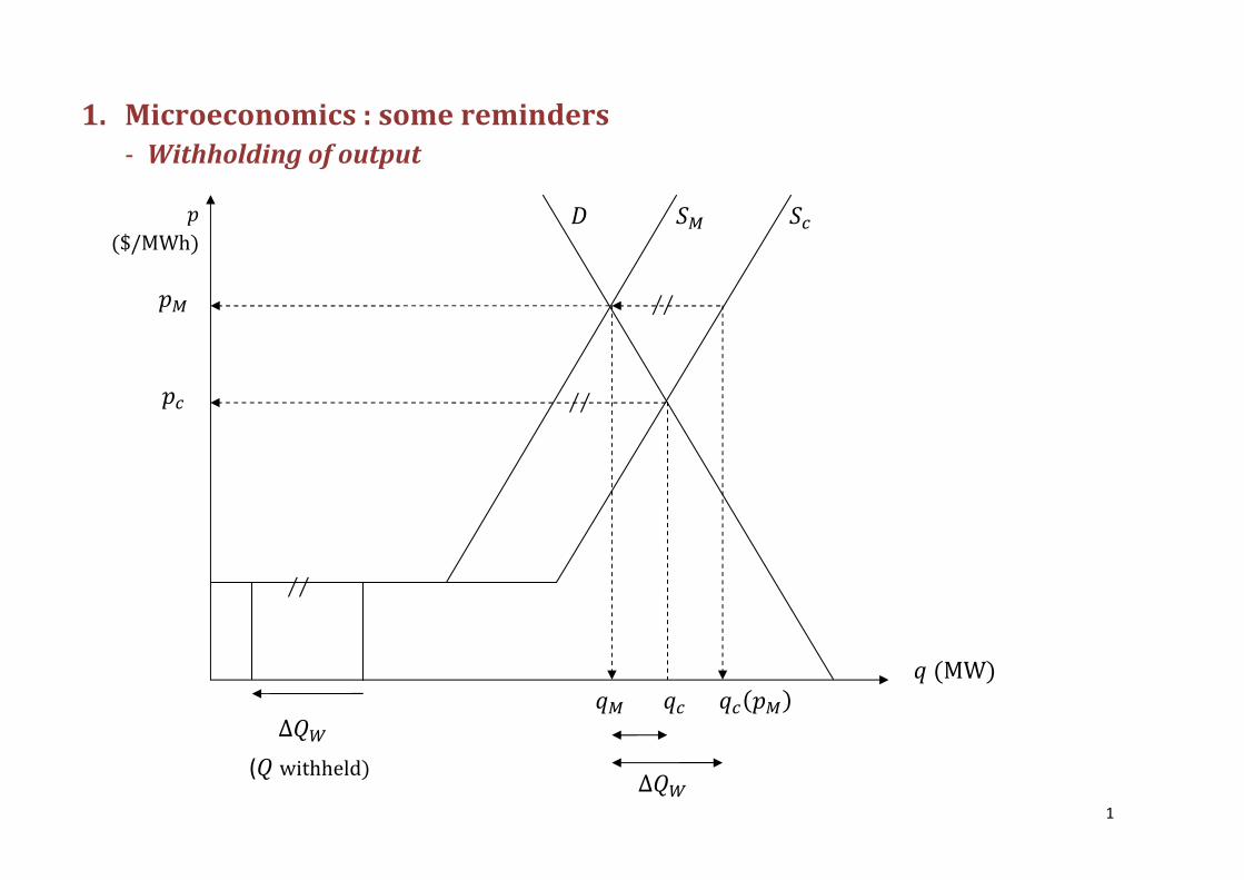
- Does it work?... Not really

9

(Counter)Example: let us imagine a power system consisting of two (types of) machines: - nuclear capacity of 40 GW with a marginal cost of c? ;

- fossil-fuel capacity of 60 GW with a marginal cost of c< 6 c? ;

- other fossil-fuel capacity spread out among a very large number of small operators;

- non-elastic demand of 50 GW.

The market price will be �P � Q<.

In the case of a nuclear duopoly, for example, where each operator has a 40% market share with the remainder being held by numerous small operators, we will obtain:

778 � �40< E �40< � 3 200.

�

100 50 40

� �MW

Q<

Q?

�P � Q<

�

10

Whereas in the case of a nuclear monopoly where the operator holds 80% of the market we calculate:

778 � �80< � 6 400.

With an identical price the HHI index varies by 100%...

- The pivotal indexes

A supplier is referred to as pivotal if the combined capacity of all its competitors is not sufficient to meet total demand. We then define:

• the PSI index (Pivotal Supplier Index) established per supplier and which has a value of 1 if the supplier is pivotal and 0 if otherwise;

• the RSI index (Residual Supply Index) established for supplier T and which is a continuous measurement calculated by means of:

,�8U � sum of the capacity of the other suppliers

quantity consumed

where ,�8U V 1 if T is pivotal.

11

The following test to gauge the level of competition is sometimes put forward: there

would be too little competition if the RSI of the biggest supplier were below 110% more

than 5% of the time.

The pertinence of these indexes is also limited. So, for example, in a system

characterized by:

- 50 GW of power in CCGT with a marginal cost of € 50/MWh;

- numerous small suppliers with in total 60 GW in low-efficiency power plants with a

marginal cost of € 100/MWh;

- and demand of 40 GW ;

there is no pivotal supplier in that system, regardless of the level of concentration of the

CCGTs.

In the case of a CCGT monopoly, we will see a price which is just under 100 and a

margin rate of 50%, despite a PSI index = 0 and RSI index = 60/40 = 150%>1.

In the case of perfect competition between CCGTs, we will see a price of € 50 and a

margin rate of zero and pivotal PSI index = 0 and RSI index = 110/40 = 275%61.

12

- Empiric illustration

RSI and Lerner Index

RSI

California, summer 2000, peak

� �$+4

/�

13

RSI

Spain, wholesale price, 2003-2005

Source : LE-GED DG Comp Study

� �$+4

/�

14

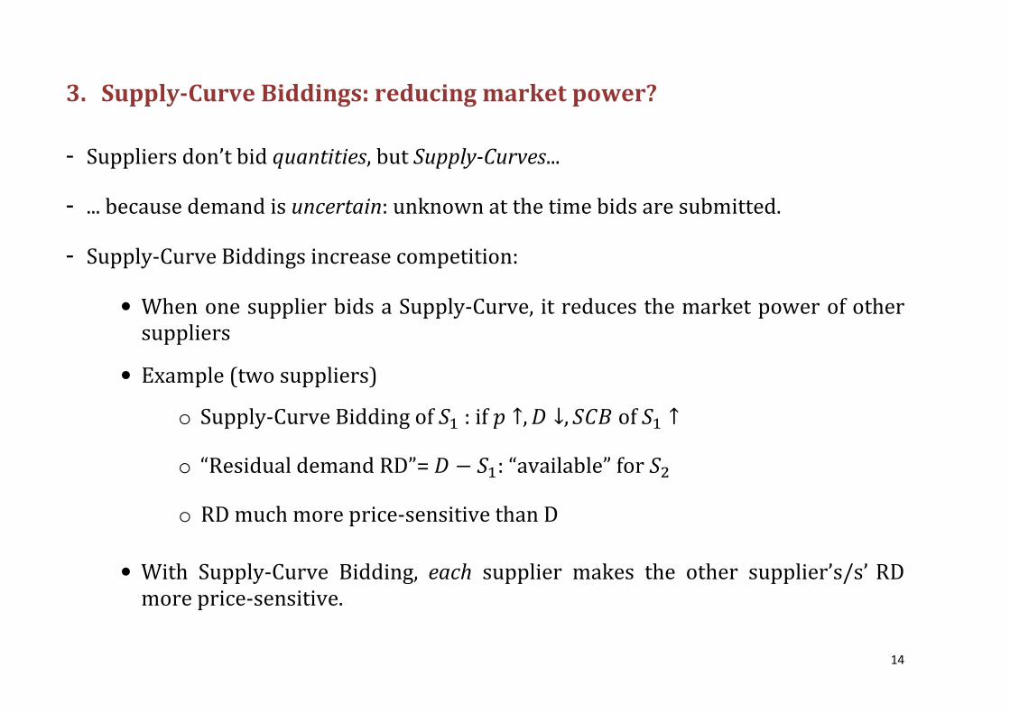
3. Supply-Curve Biddings: reducing market power?

- Suppliers don’t bid quantities, but Supply-Curves...

- ... because demand is uncertain: unknown at the time bids are submitted.

- Supply-Curve Biddings increase competition:

• When one supplier bids a Supply-Curve, it reduces the market power of other

suppliers

• Example (two suppliers)

o Supply-Curve Bidding of �? : if � W, � Y, �+Z of �? W

o “Residual demand RD”= � $ �?: “available” for �<

o RD much more price-sensitive than D

• With Supply-Curve Bidding, each supplier makes the other supplier’s/s’ RD

more price-sensitive.

15

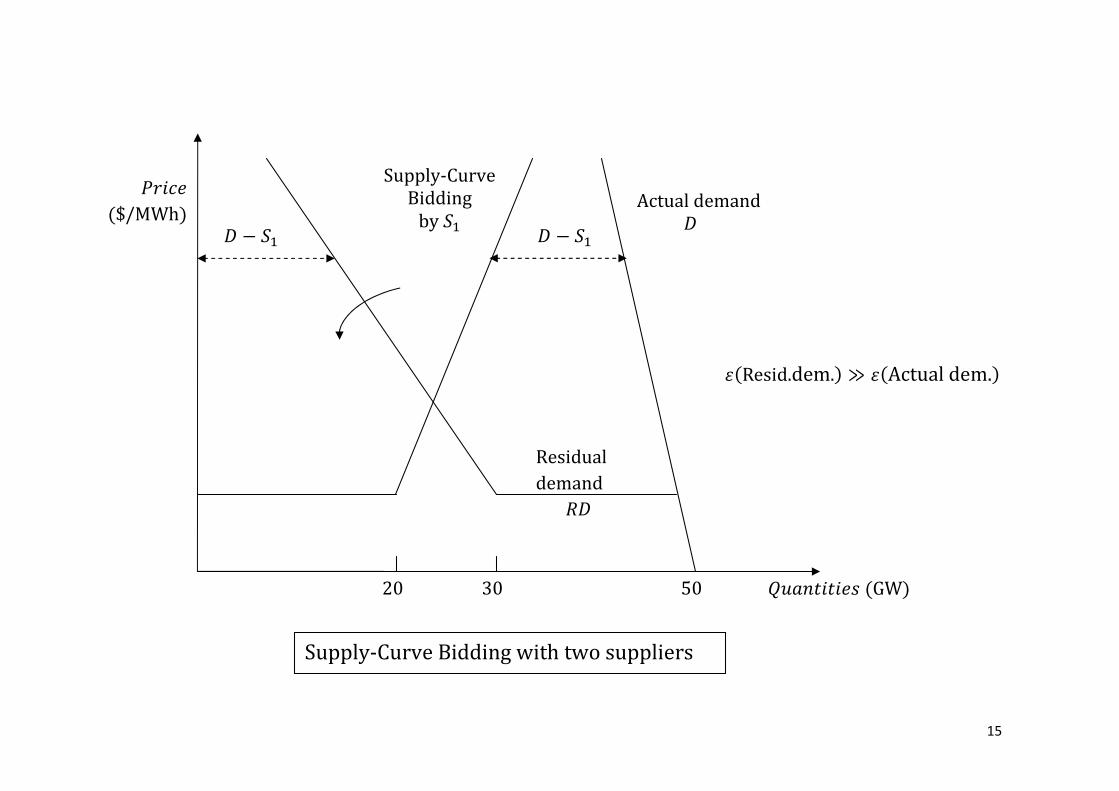
Supply-Curve Bidding with two suppliers

ij@Qk ($/MWh)

l/Am@m@k: (GW)

� $ �? Actual demand �

Supply-Curve Bidding by �?

,� Residual demand

� $ �?

20 30 50

C(Resid.dem.) s C(Actual dem.)

16

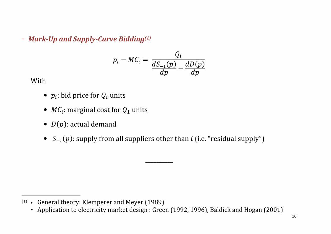
- Mark-Up and Supply-Curve Bidding(1)

�; $ !+; � ;K�D;��K� $ K��K�

With

• �;: bid price for ; units

• !+;: marginal cost for ? units

• �(�): actual demand

• �D;��: supply from all suppliers other than @ (i.e. “residual supply”)

__________

(1) • General theory: Klemperer and Meyer (1989)

• Application to electricity market design : Green (1992, 1996), Baldick and Hogan (2001)

Cases

1. Belgium

2. California

Comparison of bids with marginal costs

Marginal bid

� Highest accepted hourly sell bid or

� Highest unaccepted hourly buy bid

Hourly post-Belpex marginal costs

� Estimate of hourly marginal cost of

1

30

35

40

45

EU

R/M

Wh

Examples of marginal costs and bids

Close match, 5.2.2010� Estimate of hourly marginal cost of

the schedule cleared on Belpex

Observed results

� A variation of degree of

consistency across analyzed days

and hours

15 December, 2010

25

30

0 5 10 15 20 25

Hour

M arg inal c ost Highest accepted se ll b id

Highest unaccepted bu y bid

30

35

40

45

50

EU

R/M

Wh

0 5 10 15 20 25

Hour

Marginal cost Highest accepted sell bid

Highest unaccepted buy bid

Large difference, 8.1.2010

Comparison of bids with marginal costs

Results in Jan-Jul 2010

� General consistency (~1%

difference over the analyzed

period)

� Occasional divergence

� Absence of marginal bids during

2

Monthly marginal costs and marginal bids

40

50

� Absence of marginal bids during

off-peak hours (e.g. no accepted

buy bids or no unaccepted sell

bids)

15 December, 2010

010

20

30

40

€/M

Wh

Jan Feb Mar Apr May Jun Jul

Marginal Cost Marginal bid

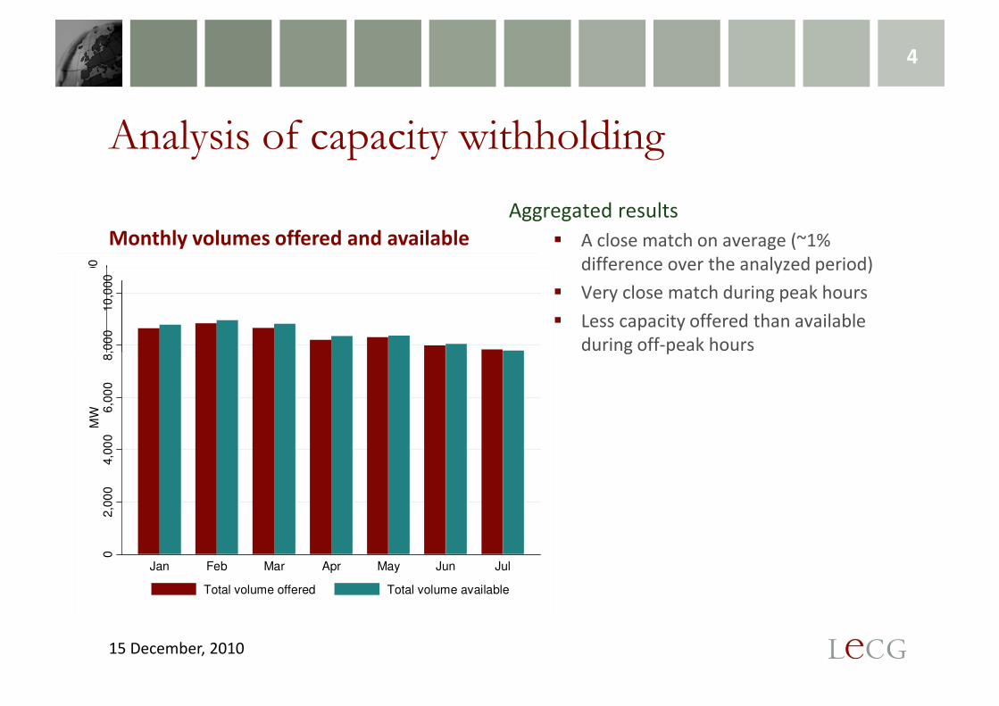
Analysis of capacity withholding

Total capacity less reserves

� Available thermal capacity and hydro

output less capacity needed to meet

the reserve requirements

Total capacity offered

� Volumes needed to meet EBL load

3

7000

8000

9000

10000

11000

MW

Examples of volumes offered and available

Close match, 25.3.2010� Volumes needed to meet EBL load

commitments, sold in Belpex and OTC,

and offered but not sold in Belpex

Observed results

� A variation of degree of consistency

across analyzed days and hours

15 December, 2010

5000

6000

0 1 2 3 4 5 6 7 8 9 10 11 12 13 14 15 16 17 18 19 20 21 22 23

Hour

Volume Offered

Volume Available

5000

6000

7000

8000

9000

10000

11000

MW

0 1 2 3 4 5 6 7 8 9 10 11 12 13 14 15 16 17 18 19 20 21 22 23

Hour

Volume Offered

Volume Available

Large difference, 5.4.2010

Analysis of capacity withholding

Aggregated results

� A close match on average (~1%

difference over the analyzed period)

� Very close match during peak hours

� Less capacity offered than available

during off-peak hours

4

8,00

010

,0

00

Monthly volumes offered and available

8,00

010

,0

00

during off-peak hours

15 December, 2010

02,00

04,00

06,00

0

MW


Total volume offered Total volume available

02,00

04,00

06,00

08,00

0

MW


Total volume offered Total volume available

California Independent System Operator

1

Predicting Market Power Using the Residual Supply Index

Presented to

FERC Market Monitoring Workshop

December 3-4, 2002

Anjali SheffrinDepartment of Market Analysis



2

Two sets of metrics to monitor market power• Measure of Market Power Impact (Price-cost markup.

Studies cited above)• Indicators of Market Structure :

• N-firm concentration or 20% Market Share• Traditional HHI• Pivotal Supplier Indicator, SMA indicator• Residual Supply Index (RSI)

What is the more accurate predictor of market power in electric markets? • Theoretical analysis and empirical study can provide guidance

Motivation and Objectives


3

Inadequacy of HHI and n-firm concentration index for electricity markets

HHI index below 2000 can mean significant price-cost markups

1-firm concentration below 20% (market based rate screen) but many firms can bid to inflate prices

Need for indicators which reflects three key factors affecting market outcomes: (1) Demand, (2) Total available supply and (3) Large suppliers’ capacity share and contract position

Development of Residual Supply Index


4

Pivotal Supplier Indicator -- A first attempt to capture the three key factorsA binary variable: whether or not a supplier is pivotal in the market given the hourly supply and demand situation. Or without this supplier, can the residual supply meet the demand?Significant improvement in predicting market power over traditional indicatorsSMA is a form of pivotal supply indicator applied to annual peak conditionInsufficiency of binary variable: ability to exercise market power when pivotal supply index close to but less than pivotalExtract further information: The RSI index

Pivotal Supplier Indicator


5

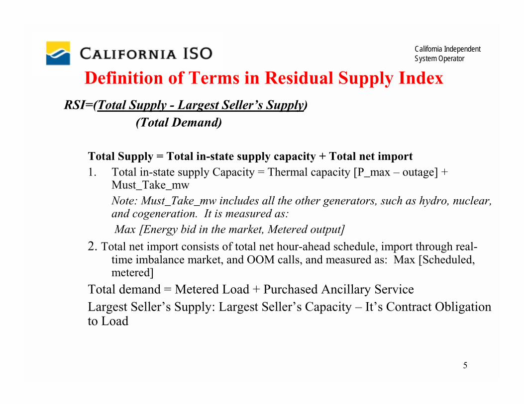
Definition of Terms in Residual Supply Index RSI=(Total Supply - Largest Seller’s Supply)

(Total Demand)

Total Supply = Total in-state supply capacity + Total net import1. Total in-state supply Capacity = Thermal capacity [P_max – outage] +

Must_Take_mwNote: Must_Take_mw includes all the other generators, such as hydro, nuclear, and cogeneration. It is measured as:Max [Energy bid in the market, Metered output]

2. Total net import consists of total net hour-ahead schedule, import through real-time imbalance market, and OOM calls, and measured as: Max [Scheduled, metered]

Total demand = Metered Load + Purchased Ancillary ServiceLargest Seller’s Supply: Largest Seller’s Capacity – It’s Contract Obligation to Load


6

Significant correlation between the Lerner Index, RSI, and actual system load

Explanation of Estimation Results

RSI versus Price-cost Markup -Summer Peak Hours, 2000

-0.40

-0.20

0.00

0.20

0.40

0.60

0.80

1.00

0.80 1.00 1.20 1.40

RSI

Pric

e-co

st M

arku

p (L

eane

r Ind

ex)


7

RSI compared with Pivotal Supplier IndexPivotal Supplier Index (and SMA) shows whether the residual supply is sufficient to meet market demand (binary index of 0 or 1)RSI shows additional information of what the ratio of residual supply relative to demand is

Residual supply / Demand

RSI or Pivotal

Pivotal Supply Index

RSI

1.0 2.00

1.0

More market power Less market power


8

Economic Rationale for RSIBased on oligopoly pricing models (such as Green and

Newberry, 1992)

Pi-MCi=Qi/(dSr(p)/dp-dD(p)/dp);Pi: bid price for Qi units of supplyMCi: marginal cost for Qi units of supplyD(p): total demand at the price of pSr: supply from all suppliers other than firm i (residual

supply)

• Qi has a positive effect on price-cost markup• Residual Supply elasticity has a negative effect on

markup• Demand elasticity has a negative effect on markup

Empirically, RSI and load are used to predict price-cost markup (demand elasticity is negligible currently, and can be incorporated later)


9

Illustration of RSI Computation for Entire Market in the Peak Hour

2000-2002 De ma nd Tota l

Supply* La rge s t Supplie r

Ca pa city**

RSI Inde x

Mus tta ke The rma l Ca pa city

Importe d Ene rgy

Ye a r (MW) (MW) (MW) (MW) (MW) (MW)

2,000 50,421 23,995 17,798 2,386 47,443 4,002 0.86

2,001 45,197 21,674 19,186 2,309 47,155 3,683 0.96

2,002 48,070 21,019 20,036 7,353 49,474 4,424 0.94

Tota l Supply

* Total supply is slightly higher than the sum of musttake, thermal capacity, and imported energy because we also account for loss adjustment.** Largest suppliers (not the same) on peak hour did not have any contract cover.


10

RSI Calculations for All HoursDuration Curve for Three Years

June-September, 2000-2002

0.8

0.9

1

1.1

1.2

1.3

1.4

1.5

1.6

1.7

1.8

1

126

251

376

501

626

751

876

1001

1126

1251

1376

1501

1626

1751

1876

2001

2126

2251

2376

2501

2626

2751

2876

frequency

RS

I in

dex

es RSI_2000RSI_2001RSI_2002

RSI_2002

RSI_2001

RSI_2000

Documents

governed by marginal cost” (J.M. Keynes, 1921)