Goodness-of-Fit â€“ Pitfalls and Power Example: Testing Consistency of Two Histograms

Goodness-of-Fit – Pitfalls and PowerExample: Testing Consistency of Two Histograms

Sometimes we have two histograms and are faced with the question:

“Are they consistent?”

That is, are our two histograms consistent with having been sampled

from the same parent distribution?

Each histogram represents a sampling from a multivariate Poisson

distribution.

0 10 20 30

010

2030

4050

60

bin index

uor

v

0 10 20 30

010

2030

4050

60

bin index

uor

v

1 Frank Porter, Caltech Seminar, February 26, 2008

Testing Consistency of Two Histograms

There are two variants of interest to this question:

1. We wish to test the hypothesis (absolute equality):

H0: The means of the two histograms are bin-by-bin equal, against

H1: The means of the two histograms are not bin-by-bin equal.

2. We wish to test the hypothesis (shape equality):

H ′0: The densities of the two histograms are bin-by-bin equal,

against

H ′1: The densities of the two histograms are not bin-by-bin equal.


Testing Consistency of Two Histograms – Some Context

There are many tests to address whether a dataset is consistent with

having been drawn from some continuous distribution.

– Histograms are built from such data. So why not work directly

with “the data”? Good question!

– Maybe original data not readily available.

– May be able to use features of binned data, eg, normal approxima-

tion ⇒ χ2.

These tests may often be adapted to address whether two datasets

have been drawn from the same continuous distribution, often called

“two-sample” tests.

These tests may then be further adapted to the present problem,

of determining whether two histograms have the same shape. Also

discussed as comparing whether two (or more) rows of a “table” are

consistent.3 Frank Porter, Caltech Seminar, February 26, 2008

Notation, Conventions

– Assume both histograms have k bins, with identical bin boundaries.

– The sampling distributions are: P (U = u) =k∏

i=1

μuii

ui!e−μi,

P (V = v) =k∏

i=1

νvii

vi!e−νi,

– Define: Nu ≡k∑

i=1Ui, μT ≡ 〈Nu〉 =

k∑i=1

μi;

Nv ≡k∑

i=1Vi, νT ≡ 〈Nv〉 =

k∑i=1

νi;

ti ≡ ui + vi, i = 1, . . . , k

Will drop distinction between random variable and realization.


Power, Confidence Level, P -value

Interested in the power of a test, for given confidence level. The

power is the probability that the null hypothesis is rejected when it is

false. Power depends on the true sampling distribution.

Power ≡ 1 − probability of a Type II error.

The confidence level is the probability that the null hypothesis is ac-

cepted, if the null hypothesis is correct.

Confidence level ≡ 1 − probability of a Type I error.

In physics, we don’t specify the confidence level of a test in advance,

at least not formally. Instead, we quote the P -value for our result. This

is the probability, under the null hypothesis, of obtaining a result as

“bad” or worse than our observed value. This would be the probability

of a Type I error if our observation were used to define the critical region

of the test.


Large Statistics Case

If all of the bin contents of both histograms are large, we use the ap-

proximation that the bin contents are normally distributed.

Under H0,

〈ui〉 = 〈vi〉 ≡ μi, i = 1, . . . , k.

More properly, it is 〈Ui〉 = μi, etc., but we are permitting ui to stand

for the random variable as well as its realization. Let the difference for

the contents of bin i between the two histograms be:

Δi ≡ ui − vi,

and let the standard deviation for Δi be denoted σi. Then the sampling

distribution of the difference between the two histograms is:

P (Δ) =1

(2π)k/2

⎛⎝ k∏

i=1

1σi

⎞⎠ exp

⎛⎝−1

2

k∑i=1

Δ2i

σ2i

⎞⎠.


Large Statistics Case – Test Statistic

This suggests the test statistic:

T =k∑

i=1

Δ2i

σ2i

.

If the σi were known, this would simply be distributed according to the

chi-square distribution with k degrees of freedom.

The maximum-likelihood estimator for the mean of a Poisson is just the

sampled number. The mean of the Poisson is also its variance, and we

will use the sampled number also as the estimate of the variance in the

normal approximation.

We’ll refer to this approach as a “χ2” test.


Large Statistics Algorithm – absolute

We suggest the following algorithm for this test:

1. For σ2i form the estimate

σ2i = (ui + vi).

2. Statistic T is thus evaluated according to:

T =k∑

i=1

(ui − vi)2

ui + vi.

If ui = vi = 0 for bin i, the contribution to the sum from that bin is

zero.

3. Estimate the P -value according to a chi-square with k degrees of free-

dom. Note that this is not an exact result.


Large Statistics Algorithm – shapes

If only comparing shapes, then scale both histogram bin contents:

1. Let N = 0.5(Nu + Nv).

Scale u and v according to:

ui → u′i = ui(N/Nu)

vi → v′i = vi(N/Nv).

2. Estimate σ2i with:

σ2i =

(N

Nu

)ui +

(N

Nv

)vi.

3. Statistic T is thus evaluated according to:

T =k∑

i=1

(uiNu

− viNv

)2

uiN2

u+ vi

N2v

.

4. Estimate the P -value according to a chi-square with k − 1 degrees of

freedom. Note that this is not an exact result.9 Frank Porter, Caltech Seminar, February 26, 2008

Application to Example0 10 20 30

010

2030

4050

60

bin index

uor

v

0 10 20 30

010

2030

4050

60

bin index

uor

v

With some small bin counts, might not expect this method to be espe-

cially good for our example, but can try it anyway:

Type of test T NDOF P (χ2 > T ) P -valueχ2 absolute comparison 53.4 36 0.031 0.023

χ2 shape comparison 38.5 35 0.31 0.28Likelihood Ratio shape comparison 38.7 35 0.31 0.35

Kolmogorov-Smirnov shape comparison 0.050 35 NA 0.22

Bhattacharyya shape comparison 0.986 35 NA 0.32

Cramer-Von-Mises shape comparison 0.193 35 NA 0.29

Anderson-Darling shape comparison 0.944 35 NA 0.42

Likelihood value shape comparison 90 35 NA 0.29Column “P -value” attempts a more reliable estimate of the probability,

under the null hypothesis, that a value for T will be as large as observed.

Compare with column P (χ2 > T ) column, the probability assuming T

follows a χ2 distribution with NDOF degrees of freedom.


Application to Example (continued)0 10 20 30

010

2030

4050

60

bin index

uor

v

0 10 20 30

010

2030

4050

60

bin index

uor

v

The absolute comparison yields much poorer agreement than the shape

comparison.

This is readily understood:

– The total number of counts in one dataset is 783; in the other it is 633.

– Treating these as samplings from a normal distribution with variances

783 and 633, we find a difference of 3.99 standard deviations or a two-

tailed P -value of 6.6 × 10−5.

– This low probability is diluted by the bin-by-bin test to 0.023.

– Lesson: The more you know about what you want to test, the better

(more powerful) the test you can make.


An Issue: We don’t know H0!

Evaluation of the probability under the null hypothesis is in fact prob-

lematic, since the null hypothesis actually isn’t completely specified.

The problem is the dependence of Poisson probabilities on the absolute

numbers of counts. Probabilities for differences in Poisson counts are

not invariant under the total number of counts.

Unfortunately, we don’t know the true mean numbers of counts in

each bin under H0. Thus, we must estimate these means.

The procedure adopted here has been to use the maximum likelihood

estimators (see later) for the mean numbers, in the null hypothesis.

We’ll have further discussion of this procedure below – It does not always

yield valid results.


Use of chi-square Probability Distribution

In our example, the probabilities estimated according to our simula-

tion and the χ2 distribution probabilities are fairly close to each other.

Suggests the possibility of using the χ2 probabilities – if we can do this,

the problem that we haven’t completely specified the null hypothesis is

avoided.

Conjecture: Let T be the “χ2” test statistic, for either the absolute or the

shape comparison, as desired. Let Tc be a possible value of T (perhaps

the critical value to be used in a hypothesis test). Then, for large values

of Tc, under H0 (or H ′0):

P (T < Tc) ≥ P(T < Tc|χ2(T,ndof)

),

where P(T < Tc|χ2(T,ndof)

)is the probability that T < Tc according

to a χ2 distribution with ndof degrees of freedom (either k or k − 1,

depending on which test is being performed).


Is it Useful?

The conjecture tells us that if we use the probabilities from a χ2 dis-

tribution in our test, the error that we make is in the “conservative”

direction.

That is, we’ll reject the null hypothesis less often than we would with

the correct probability.

This conjecture is independent of the statistics of the sample, bins

with zero counts are fine. In the limit of large statistics, the inequality

approaches equality.

Unfortunately, it isn’t as nice as it sounds. The problem is that, in low

statistics situations, the power of the test according to this approach can

be dismal. We might not reject the null hypothesis in situations where

it is obviously implausible.


Is it Useful? (continued)

60 80 100 120 140Tc

60 80 100 120 14060 80 100 120 140

0.0

0.2

0.4

0.6

0.8

1.0

Tc

Pro

babi

lity(

T<

Tc)

60 80 100 120 140

0.0

0.2

0.4

0.6

0.8

1.0

60 80 100 120 140Tc

60 80 100 120 140

(a) (b) (c)

Comparison of actual (cumulative) probability distribution for T (solid

blue curves) with chi-square distribution (dashed red curves). All plots

are for 100 bin histograms, and null hypothesis:

(a) Each bin has mean 100.

(b) Each bin has mean 1.

(c) Bin j has mean 30/j.


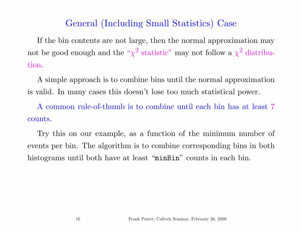
General (Including Small Statistics) Case

If the bin contents are not large, then the normal approximation may

not be good enough and the “χ2 statistic” may not follow a χ2 distribu-

tion.

A simple approach is to combine bins until the normal approximation

is valid. In many cases this doesn’t lose too much statistical power.

A common rule-of-thumb is to combine until each bin has at least 7

counts.

Try this on our example, as a function of the minimum number of

events per bin. The algorithm is to combine corresponding bins in both

histograms until both have at least “minBin” counts in each bin.


Combining bins for χ2 test

0 10 20 30

010

2030

4050

60

bin index

uor

v

0 10 20 30

010

2030

4050

60

bin index

uor

v

0

5

10

15

20

25

30

35

40

0 20 40 60 80 100 120 140minBin

T or

k0

0.1

0.2

0.3

0.4

0.5

0 20 40 60 80 100 120 140minBin

Pro

babi

lity

Left: The example pair of histograms.

Middle: The solid curve shows the value of the test statistic T , and the

dashed curve shows the number of histogram bins for the data in the

example, as a function of the minimum number of counts per bin.

Right: The P -value for consistency of the two datasets in the example.

The solid curve shows the probability for a chi-square distribution, and

the dashed curved shows the probability for the actual distribution, with

an estimated null hypothesis.


Working with the Poissons - Normalization Test

Alternative: Work with the Poisson distribution. Separate the problem

of the shape from that of the overall normalization.

To test normalization, compare totals over all bins between the his-

tograms. Distribution isP (Nu,Nv) =

μNuT νNv

T

Nu!Nv!e−(μT+νT ).

The null hypothesis is H0 : μT = νT , to be tested against alternative

H1 : μT = νT . We are interested in the difference between the two

means; the sum is a nuisance parameter. Hence, consider:

P (Nv|Nu + Nv = N) =P (N |Nv)P (Nv)

P (N)

=μN−Nv

T e−μT

(N − Nv)!νNvT e−νT

Nv!/(μT + νT )Ne−(μT+νT )

N !

=(

NNv

) (νT

μT + νT

)Nv(

μT

μT + νT

)N−Nv

.Example of use of con-

ditional likelihood.


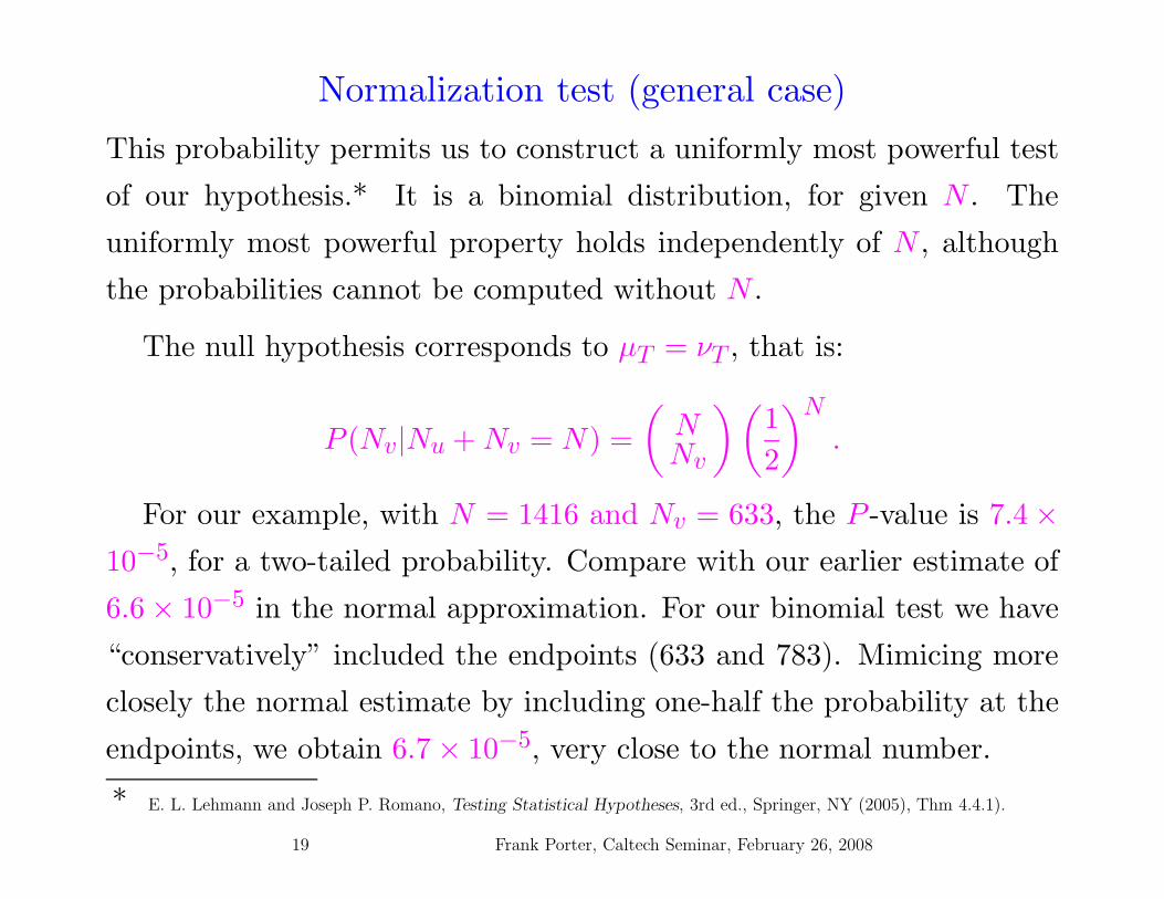
Normalization test (general case)

This probability permits us to construct a uniformly most powerful test

of our hypothesis.* It is a binomial distribution, for given N . The

uniformly most powerful property holds independently of N , although

the probabilities cannot be computed without N .

The null hypothesis corresponds to μT = νT , that is:

P (Nv|Nu + Nv = N) =(

NNv

) (12

)N

.

For our example, with N = 1416 and Nv = 633, the P -value is 7.4 ×10−5, for a two-tailed probability. Compare with our earlier estimate of

6.6 × 10−5 in the normal approximation. For our binomial test we have

“conservatively” included the endpoints (633 and 783). Mimicing more

closely the normal estimate by including one-half the probability at the

endpoints, we obtain 6.7 × 10−5, very close to the normal number.

* E. L. Lehmann and Joseph P. Romano, Testing Statistical Hypotheses, 3rd ed., Springer, NY (2005), Thm 4.4.1).


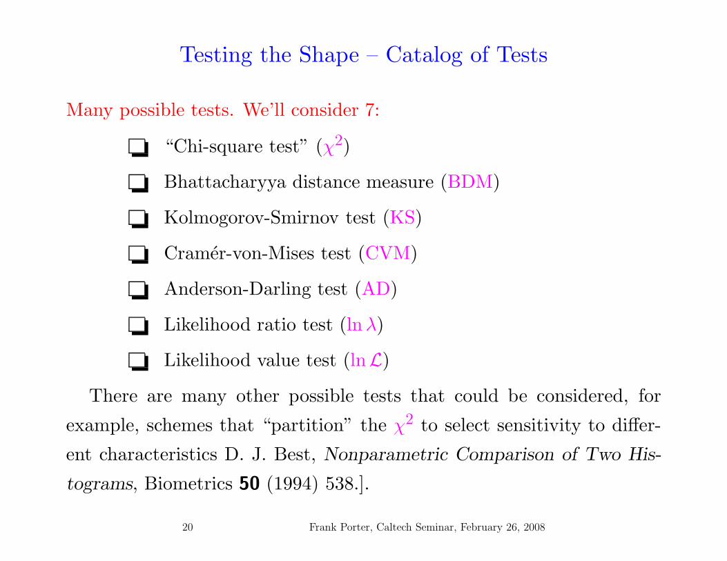
Testing the Shape – Catalog of Tests

Many possible tests. We’ll consider 7:

“Chi-square test” (χ2)

Bhattacharyya distance measure (BDM)

Kolmogorov-Smirnov test (KS)

Cramer-von-Mises test (CVM)

Anderson-Darling test (AD)

Likelihood ratio test (lnλ)

Likelihood value test (lnL)

There are many other possible tests that could be considered, for

example, schemes that “partition” the χ2 to select sensitivity to differ-

ent characteristics D. J. Best, Nonparametric Comparison of Two His-

tograms, Biometrics 50 (1994) 538.].


Chi-square test for shape

Even though we don’t expect it to follow a χ2 distribution in the low

statistics regime, we may evaluate the test statistic:

χ2 =k∑

i=1

(uiNu

− viNv

)2

uiN2

u+ vi

N2v

.

If ui = vi = 0, the contribution to the sum from that bin is zero.


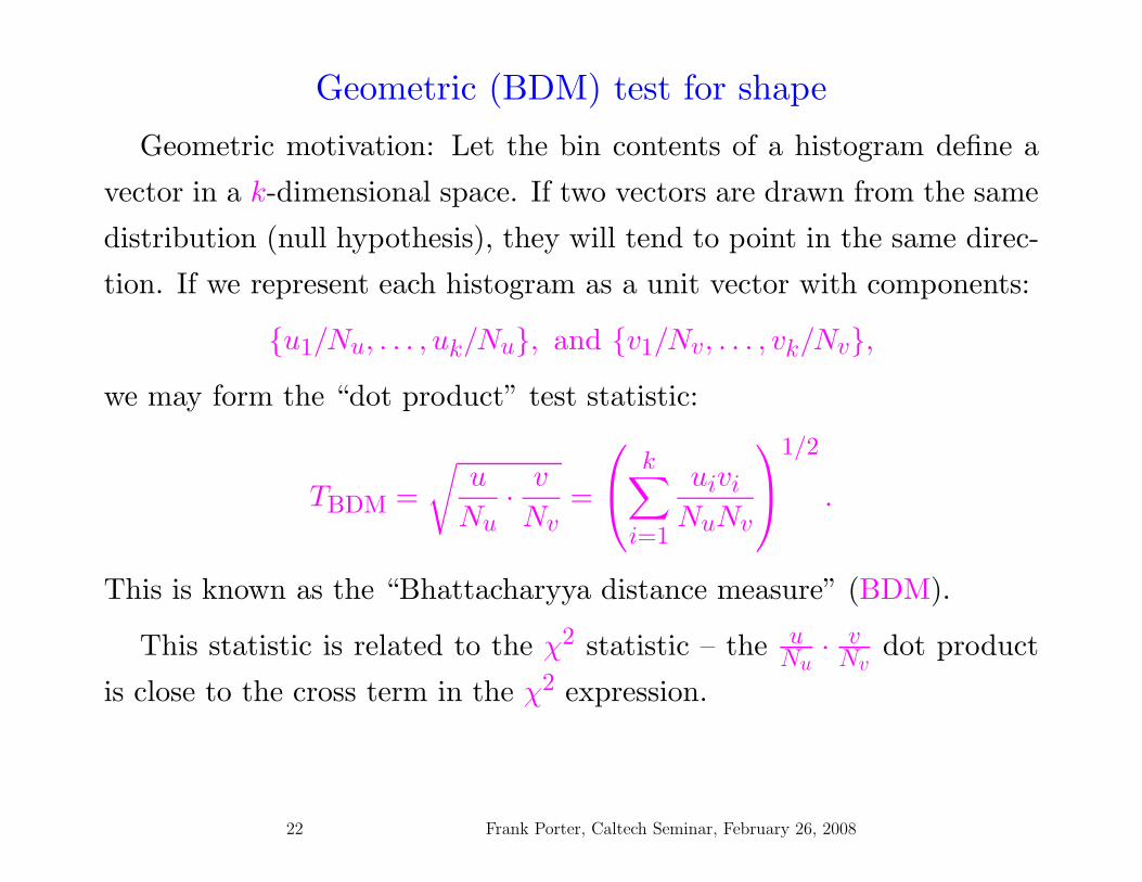
Geometric (BDM) test for shape

Geometric motivation: Let the bin contents of a histogram define a

vector in a k-dimensional space. If two vectors are drawn from the same

distribution (null hypothesis), they will tend to point in the same direc-

tion. If we represent each histogram as a unit vector with components:

{u1/Nu, . . . , uk/Nu}, and {v1/Nv, . . . , vk/Nv},we may form the “dot product” test statistic:

TBDM =√

u

Nu· v

Nv=

⎛⎝ k∑

i=1

uivi

NuNv

⎞⎠

1/2

.

This is known as the “Bhattacharyya distance measure” (BDM).

This statistic is related to the χ2 statistic – the uNu

· vNv

dot product

is close to the cross term in the χ2 expression.


Sample application of BDM test

Apply this formalism to our example. The sum over bins gives 0.986.

According to our estimated distribution of this statistic under the null

hypothesis, this gives a P -value of 0.32, similar to the χ2 test result

(0.28).

0 10 20 30

0.00

0.02

0.04

0.06

0.08

0.10

Bin index

BDM

per

bin

Bin-by-bin contributions to the

BDM test statistic for the exam-

ple.

BDM statisticFr

eque

ncy

0.970 0.975 0.980 0.985 0.990 0.995

050

010

0015

0020

0025

00Estimated distribution of the BDM

statistic for the null hypothesis

in the example.


Kolmogorov-Smirnov test

Another approach to a shape test may be based

on the Kolmogorov-Smirnov (KS) idea: Esti-

mate the maximum difference between observed

and predicted cumulative distribution functions

and compare with expectations.6 8 10 12

0.0

0.2

0.4

0.6

0.8

1.0

x

CD

F

Modify the KS statistic to apply to comparison of histograms: As-

sume neither histogram is empty. Form the “cumulative distribution

histograms” according to:

uci =i∑

j=1uj/Nu vci =

i∑j=1

vj/Nv.

Then compute the test statistic (for a two-tail test):

TKS = maxi

|uci − vci|.24 Frank Porter, Caltech Seminar, February 26, 2008

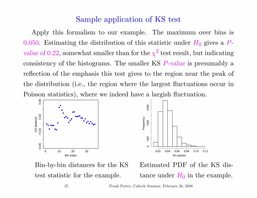
Sample application of KS test

Apply this formalism to our example. The maximum over bins is

0.050. Estimating the distribution of this statistic under H0 gives a P -

value of 0.22, somewhat smaller than for the χ2 test result, but indicating

consistency of the histograms. The smaller KS P -value is presumably a

reflection of the emphasis this test gives to the region near the peak of

the distribution (i.e., the region where the largest fluctuations occur in

Poisson statistics), where we indeed have a largish fluctuation.

0 10 20 30

−0.

06−

0.02

0.02

0.06

Bin index

KS

dis

tanc

e

Bin-by-bin distances for the KS

test statistic for the example.

KS statistic

Freq

uenc

y

0.02 0.04 0.06 0.08 0.10 0.120

500

1500

2500

Estimated PDF of the KS dis-

tance under H0 in the example.25 Frank Porter, Caltech Seminar, February 26, 2008

Cramer-von-Mises test

The idea of the Cramer-von-Mises (CVM) test is to add up the squared

differences between the cumulative distributions being compared. Used

to compare an observed distribution with a presumed parent continu-

ous probability distribution. Algorithm is adaptable to the two-sample

comparison, and to the case of comparing two histograms.

The test statistic for comparing the two samples x1, x2, . . . , xN and

y1, y2, . . . , yM is*:

T =NM

(N + M)2

⎧⎨⎩

N∑i=1

[Ex(xi) − Ey(xi)

]2 +M∑

j=1

[Ex(yj) − Ey(yj)

]2⎫⎬⎭ ,

where Ex is the empirical cumulative distribution for sampling x. That

is, Ex(x) = n/N if n of the sampled xi are less than or equal to x.

* T. W. Anderson, On the Distribution of the Two-Sample Cramer-Von Mises Criterion, Ann. Math. Stat. 33 (1962) 1148.


Cramer-von-Mises test – Adaptation to comparing histograms

Adapt this for the present application of comparing histograms with

bin contents u1, u2, . . . , uk and v1, v2, . . . , vk with identical bin bound-

aries: Let z be a point in bin i, and define the empirical cumulative

distribution function for histogram u as:

Eu(z) =i∑

j=1ui/Nu.

Then the test statistic is:

TCVM =NuNv

(Nu + Nv)2

k∑j=1

(uj + vj)[Eu(zj) − Ev(zj)

]2.


Sample application of CVM test

Apply this formalism to our example, finding TCVM = 0.193. The re-

sulting estimated distribution under the null hypothesis is shown below.


hypothesis, this gives a P -value of 0.29, similar with the χ2 test result.

0 10 20 30

010

2030

4050

60

bin index

uor

v

0 10 20 30

010

2030

4050

60

bin index

uor

v

CVM statistic

Freq

uenc

y0.0 0.5 1.0 1.5

020

0040

00

Example. Estimated PDF of the CVM statis-

tic under H0 for the example.


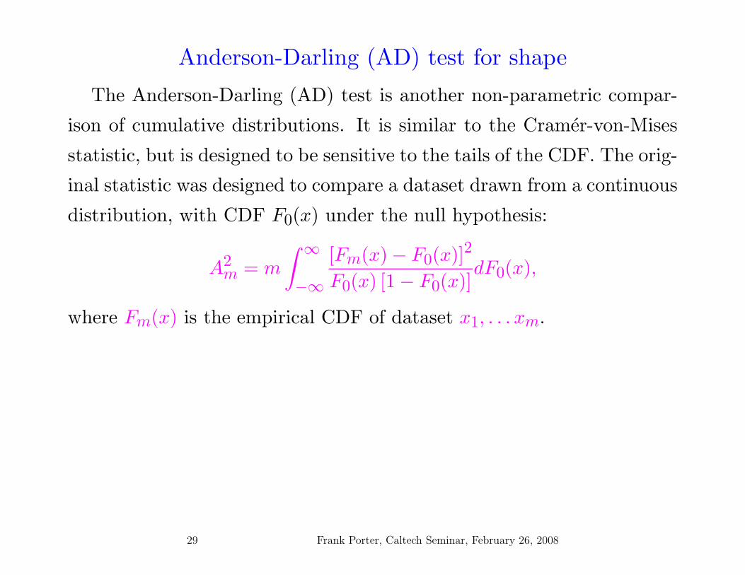
Anderson-Darling (AD) test for shape

The Anderson-Darling (AD) test is another non-parametric compar-

ison of cumulative distributions. It is similar to the Cramer-von-Mises

statistic, but is designed to be sensitive to the tails of the CDF. The orig-

inal statistic was designed to compare a dataset drawn from a continuous

distribution, with CDF F0(x) under the null hypothesis:

A2m = m

∫ ∞

−∞[Fm(x) − F0(x)]2

F0(x) [1 − F0(x)]dF0(x),

where Fm(x) is the empirical CDF of dataset x1, . . . xm.


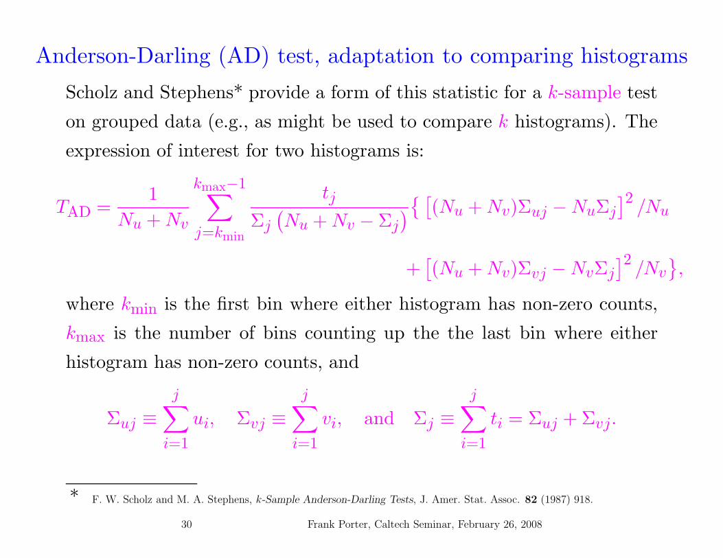
Anderson-Darling (AD) test, adaptation to comparing histograms

Scholz and Stephens* provide a form of this statistic for a k-sample test

on grouped data (e.g., as might be used to compare k histograms). The

expression of interest for two histograms is:

TAD =1

Nu + Nv

kmax−1∑j=kmin

tj

Σj(Nu + Nv − Σj

){ [(Nu + Nv)Σuj − NuΣj

]2/Nu

+[(Nu + Nv)Σvj − NvΣj

]2/Nv

},

where kmin is the first bin where either histogram has non-zero counts,

kmax is the number of bins counting up the the last bin where either

histogram has non-zero counts, and

Σuj ≡j∑

i=1ui, Σvj ≡

j∑i=1

vi, and Σj ≡j∑

i=1ti = Σuj + Σvj.

* F. W. Scholz and M. A. Stephens, k-Sample Anderson-Darling Tests, J. Amer. Stat. Assoc. 82 (1987) 918.


Sample application of AD test for shape

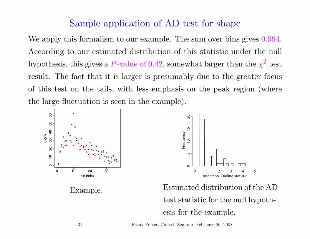
We apply this formalism to our example. The sum over bins gives 0.994.


hypothesis, this gives a P -value of 0.42, somewhat larger than the χ2 test

result. The fact that it is larger is presumably due to the greater focus

of this test on the tails, with less emphasis on the peak region (where

the large fluctuation is seen in the example).

0 10 20 30

010

2030

4050

60

bin index

uor

v

0 10 20 30

010

2030

4050

60

bin index

uor

v

Anderson−Darling statistic

Freq

uenc

y

0 1 2 3 4 5

05

1015

20Example. Estimated distribution of the AD

test statistic for the null hypoth-

esis for the example.31 Frank Porter, Caltech Seminar, February 26, 2008

Likelihood ratio test for shape

Base a shape test on the same conditional likelihood idea as for the

normalization test. Now there is a binomial associated with each bin.

The two histograms are sampled from the joint distribution:

P (u, v) =k∏

i=1

μuii

ui!e−μi

νvii

vi!e−νi.

With ti = ui + vi, and fixing the ti at the observed values, we have

the multi-binomial form:

P (v|u + v = t) =k∏

i=1

(tivi

)(νi

νi + μi

)vi(

μi

νi + μi

)ti−vi

.


Likelihood ratio test for shape (continued)

The null hypothesis is νi = aμi, i = 1, . . . , k. We want to test this,

but there are two complications:

1. The value of “a” is not specified;

2. We still have a multivariate distribution.

For a, we substitute the maximum likelihood estimator:

a =Nv

Nu.

Use a likelihood ratio statistic to reduce the problem to a single vari-

able. This will be the likelihood under the null hypothesis (with a given

by its maximum likelihood estimator), divided by the maximum of the

likelihood under the alternative hypothesis.


Likelihood ratio test for shape (continued)

We form the ratio:

λ =maxH0 L(a|v; u + v = t)

maxH1 L({ai ≡ νi/μi}|v; u + v = t)=

k∏i=1

(a

1+a

)vi(

11+a

)ti−vi

(ai

1+ai

)vi(

11+ai

)ti−vi.

The maximum likelihood estimator, under H1, for ai is just ai = vi/ui.

Thus, we rewrite our test statistic as: λ =k∏

i=1

(1 + vi/ui

1 + Nv/Nu

)ti(

Nv

Nu

ui

vi

)vi

.

In practice, we’ll work with

−2 ln λ = −2k∑

i=1

[ti ln

(1 + vi/ui

1 + Nv/Nu

)+ vi ln

(Nv

Nu

ui

vi

)].

If ui = vi = 0, the bin contributes zero.

If vi = 0, contribution is −2 lnλi = −2ti ln(

NuNu+Nv

).

If ui = 0, the contribution is −2 lnλi = −2ti ln(

NvNu+Nv

).


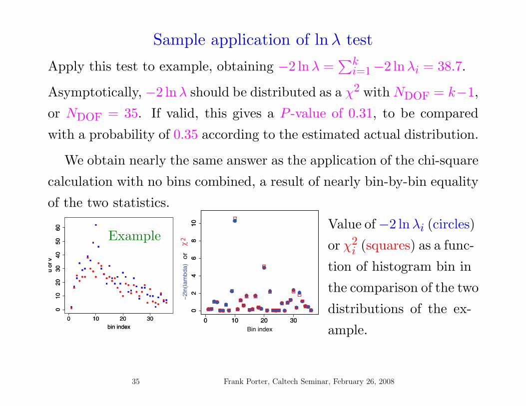
Sample application of lnλ test

Apply this test to example, obtaining −2 lnλ =∑k

i=1−2 lnλi = 38.7.

Asymptotically, −2 lnλ should be distributed as a χ2 with NDOF = k−1,

or NDOF = 35. If valid, this gives a P -value of 0.31, to be compared

with a probability of 0.35 according to the estimated actual distribution.

We obtain nearly the same answer as the application of the chi-square

calculation with no bins combined, a result of nearly bin-by-bin equality

of the two statistics.

0 10 20 30

010

2030

4050

60

bin index

uor

v

0 10 20 30

010

2030

4050

60

bin index

uor

v

Example

or

2χ

Value of −2 ln λi (circles)

or χ2i (squares) as a func-

tion of histogram bin in

the comparison of the two

distributions of the ex-

ample.


Comparison of lnλ and χ2

To investigate when this might hold more generally, compare the val-

ues of −2 lnλi and χ2i as a function of ui and vi, below. The two statis-

tics agree when ui = vi with increasing difference away from that point.

This agreement holds even for low statistics. However, shouldn’t con-

clude that the chi-square approximation may be used for low statistics

– fluctuations away from equal numbers lead to quite different results

when we get into the tails at low statistics. Our example doesn’t really

sample these tails – the only bin with a large difference is already high

statistics.

Value of −2 lnλi or χ2i as a func-

tion of ui and vi bin contents.

This plot assumes Nu = Nv. 0

2

4

6

8

10

12

14

16

0 2 4 6 8 10v

T

chisq, u=0-2lnL, u=0chisq, u=5-2lnL, u=5chisq, u=10-2lnL, u=10


Likelihood value test

– Let lnL be the value of the likelihood at its maximum value under

the null hypothesis.

– lnL is an often-used but controversial goodness-of-fit statistic.

– Can be demonstrated that this statistic carries little or no information

in some situations.

– However, in the limit of large statistics it is essentially the chi-square

statistic, so there are known situations were it is a plausible statistic

to use.

– Using the results in the previous slides, the test statistic is:

lnL = −k∑

i=1

[ln

(tivi

)+ ti ln

Nu

Nu + Nv+ vi ln

Nv

Nu

].

If either Nu = 0 or Nv = 0, then lnL = 0.


Sample application of the lnL test

– Apply this test to the example. The sum over bins is 90. Using our

estimated distribution of this statistic under the null hypothesis, this

gives a P -value of 0.29, similar to the χ2 test result.

– To be expected, since our example is reasonably well-approximated

by the large statistics limit.

ln Likelihood

Fre

quen

cy

75 80 85 90 95 100 105

050

010

0015

0020

00

Estimated distribution of the lnL test statistic under H0 in the ex-

ample.


Distributions Under the Null Hypothesis

Our example may be too easy. . .

When the asymptotic distribution may not be good enough, we would

like to know the probability distribution of our test statistic under the

null hypothesis.

Difficulty: our null hypothesis is not completely specified!

The problem is that the distribution depends on the values of νi = aμi.

Our null hypothesis only says νi = aμi, but says nothing about what μi

might be.

[It also doesn’t specify a, but we have already discussed that compli-

cation, which appears manageable.]


Estimating the null hypothesis

– Turn to the data to make an estimate for μi, to be used in estimating

the distribution of our test statistics.

– Straightforward approach: use the M.L. parameter estimators (under

H0):

μi =1

1 + a(ui + vi),

where a = Nv/Nu

νi =a

1 + a(ui + vi).

– Repeatedly simulate data using these values for the parameters of the

sampling distribution.

– For each simulation, obtain a value of the test statistic.

– The distribution so obtained is then an estimate of the distribution of

the test statistic under H0, and P -values may be computed from this.


But it isn’t guaranteed to work. . .

– We have just described the approach that was used to compute the

estimated probabilities for the example. The bin contents are reason-

ably large, and this approach works well enough for this case.

– Unfortunately, this approach can do very poorly in the low-statistics

realm.

– Consider a simple test case: Suppose our data is sampled from a flat

distribution with a mean of 1 count in each of 100 bins.


Algorithm to check estimated null hypothesis

We test how well our estimated null hypothesis works for any given

test statistic, T , as follows:

1. Generate a pair of histograms according to some assumed H0.

(a) Compute T for this pair of histograms.

(b) Given the pair of histograms, compute the estimated null hypoth-

esis according to the specified prescription above.

(c) Generate many pairs of histograms according to the estimated null

hypothesis in order to obtain an estimated distribution for T .

(d) Using the estimated distribution for T , determine the estimated

P -value for the value of T found in step (a).

2. Repeat step 1 many times and make a histogram of the estimated P -

values. This histogram should be uniform if the estimated P -values

are good estimates.


Checking the estimated null distribution

The next two slides show tests of the estimated null distribution for

each the 7 test statistics.

Shown are distributions of the simulated P -values. The data are gener-

ated according to H0, consisting of 100 bin histograms for:

– A mean of 100 counts/bin (left column), or

– A mean of 1 count/bin (other 3 columns).

The estimates of H0 are:

– Weighted bin-by-bin average (left two columns),

– Each bin mean given by the average bin contents in each histogram

(third column),

– Estimated with a Gaussian kernel estimator (right column) based on

the contents of both histograms.

The χ2 is computed without combining bins.


05

1015

2025

05

1015

2025

300

510

1520

250

510

15

20

25

Estimated probability0.0 0.2 0.4 0.6 0.8 1.0

Fre

quen

cy0

510

1520

25

05

015

025

0

Fre

quen

cy0

510

1520

25

05

010

020

0

Fre

quen

cy0

510

1520

25

05

1015

2025

30

Fre

quen

cy0

510

15

20

25

05

101

52

02

53

0



2χ

BDM

KS

CVM

05

1015

2025

300

510

1520

2530

05

1015

2025

05

1015

2025

30


<counts/bin> = 100 <counts/bin> = 1

H0 is weighted bin-by-bin average H0 from overall average H0 from Gaussian kernel estimator


05

1015

2025

300

510

1520

2530


01

02

03

0

Fre

quen

cy0

510

1520

2530

05

1015

2025

30

Fre

quen

cy0

510

1520

25

010

020

030

040

0

Estimated probability

Fre

quen

cy

0.0 0.2 0.4 0.6 0.8 1.0

05

1015

2025

30


010

020

030

040

0

AD

ln

ln

λ

L

05

1015

2025

300

510

1520

2530


010

2030

<counts/bin> = 100 <counts/bin> = 1

H0 is weighted bin-by-bin average H0 from overall average H0 from Gaussian kernel estimator


Summary of tests of null distribution estimates

Probability that the null hypothesis will be rejected with a cut at 1%

on the estimated distribution. H0 is estimated with the bin-by-bin al-

gorithm in the first two columns, by the uniform histogram algorithm

in the third column, and by Gaussian kernel estimation in the fourth

column.

Test statistic Probability (%) Probability (%) Probability (%) Probability (%)Bin mean = 100 1 1 1

H0 estimate bin-by-bin bin-by-bin uniform kernelχ2 0.97 ± 0.24 18.5 ± 1.0 1.2 ± 0.3 1.33 ± 0.28

BDM 0.91 ± 0.23 16.4 ± 0.9 0.30 ± 0.14 0.79 ± 0.22

KS 1.12 ± 0.26 0.97 ± 0.24 1.0 ± 0.2 1.21 ± 0.27

CVM 1.09 ± 0.26 0.85 ± 0.23 0.8 ± 0.2 1.27 ± 0.28

AD 1.15 ± 0.26 0.85 ± 0.23 1.0 ± 0.2 1.39 ± 0.29

lnλ 0.97 ± 0.24 24.2 ± 1.1 1.5 ± 0.3 2.0 ± 0.34

lnL 0.97 ± 0.24 28.5 ± 1.1 0.0 ± 0.0 0.061 ± 0.061


Conclusions from tests of null distribution estimates

In the “large statistics” case, where sampling is from histograms with

a mean of 100 counts in each bin, all test statistics display the desired

flat distribution.

The χ2, lnλ, and lnL statistics perform essentially identically at high

statistics, as expected, since in the normal approximation they are

equivalent.

In the “small statistics” case, if the null hypothesis were to be re-

jected at the estimated 0.01 probability, the bin-by-bin algortihm for

estimating ai would actually reject H0: 19% of the time for the χ2

statistic, 16% of the time for the BDM statistic, 24% of the time for

the lnλ statistic, and 29% of the time for the L statistics, all unac-

ceptably larger than the desired 1%. The KS, CVM, and AD statistics

are all consistent with the desired 1%.


Problem appears for low statistics

Intuition behind the failure of the bin-by-bin approach at low statistics:

Consider the likely scenario that some bins will have zero counts in both

histograms. Then our algorithm for the estimated null hypothesis yields

a zero mean for these bins. The simulation to determine the probability

distribution for the test statistic will always have zero counts in these

bins, ie, there will always be agreement between the two histograms.

Thus, the simulation will find that low values of the test statistic are

more probable than it should.

The AD, CVM, and KS tests are more robust under our estimates

of H0 than the others, as they tend to emphasize the largest differences

and are not so sensitive to bins that always agree. For these statistics,

our bin-by-bin procedure for estimating H0 does well even for low statis-

tics, although we caution that we are not examining the far tails of the

distribution.


Obtaining better null distribution estimates

A simple approach to salvaging the situation in the low statistics

regime involves relying on the often valid assumption that the un-

derlying H0 distribution is “smooth”. Then only need to estimate a

few parameters to describe the smooth distribution, and effectively

more statistics are available.

Assuming a smooth background represented by a uniform distribution

yields correct results. This is cheating a bit, since we aren’t supposed

to know that this is really what we are sampling from.

The lnL and to a lesser extent the BDM statistic, do not give the

desired 1% result, but now err on the “conservative” side. May be

possible to mitigate this with a different algorithm. Expect the power

of these statistics to suffer under the approach taken here.


More “honest” – Try a kernel estimator

Since we aren’t supposed to know that our null distribution is uniform,

we also try a kernel estimator for H0, using the sum of the observed

histograms as input. Try a Gaussian kernel, with a standard deviation

of 2. It works pretty well, though there is room for improvement. The

bandwidth was chosen here to be rather small for technical reasons; a

larger bandwidth might improve results.

0 20 40 60 80 1000.00

40.

008

0.01

20.

016

bin

Den

sity

Sample Gaussian kernel density estimate of the null hypothesis.50 Frank Porter, Caltech Seminar, February 26, 2008

Comparison of Power of Tests

The power depends on what the alternative hypothesis is.

Investigate adding a Gaussian component on top of a uniform back-

ground distribution. Motivated by the scenario where one distribution

appears to show some peaking structure, while the other does not.

Also look at a different extreme, a rapidly varying alternative.


Gaussian alternaitve

The Gaussian alternative data are generated as follows:

The “background” has a mean of one event per histogram bin.

The Gaussian has a mean of 50 and a standard deviation of 5, in units

of bin number.

As a function of the amplitude of the Gaussian, count how often the

null hypothesis is rejected at the 1% confidence level. The amplitude

is measured in percent, eg, a 25% Gaussian has a total amplitude cor-

responding to an average of 25% of the total counts in the histogram.

The Gaussian counts are added to the counts from the background

distribution.


Sample Gaussian alternative

0 20 40 60 80 100

1.0

1.5

2.0

2.5

3.0

3.5

Bin number

Mea

n c

ou

nts

/bin

0 20 40 60 80 100

01

23

45

67

0 20 40 60 80 100

01

23

45

67

Bin number

Co

un

ts/b

inLeft: The mean bin contents for a 25% Gaussian on a flat background

of one count/bin (note the suppressed zero).

Right: Example sampling from the 25% Gaussian (filled blue dots) and

from the uniform background (open red squares).


Power estimates for Gaussian alternative

On the next two slides, we show, for seven test statistics, the distribution

of the estimated probability, under H0, that the test statistic is worse

than that observed.

Three different magnitudes of the Gaussian amplitude are displayed.

The data are generated according to a uniform distribution, consisting

of 100 bin histograms with a mean of 1 count, for one histogram, and

for the other histogram with an added Gaussian peak of strength:

– 12.5% (left column),

– 25% (middle column), and

– 50% (right column).

[The χ2 is computed without combining bins.]


Fre

quen

cy0

510

1520

2530

01

03

05

07

0

010

020

030

040

050

0

12.5% 25% 50%2χ

Fre

quen

cy0

510

1520

2530

01

02

03

04

0

010

030

050

0BDMF

requ

ency

01

02

03

04

05

06

0

05

010

015

020

0

05

0010

0015

00

KS

Fre

quen

cy0

10

20

30

40

02

04

06

08

0

050

010

0015

00

CVM





05

0010

0015

00

Fre

quen

cy0

10

20

30

40

02

04

06

08

010

0

AD

020

040

060

080

0

Fre

quen

cy0

10

20

30

02

04

06

08

010

0

lnλ


010

020

030

040

050

0

Estimated probability

Fre

quen

cy

0.0 0.2 0.4 0.6 0.8 1.0

05

1020

30


01

02

03

0

lnL

12.5% 25% 50%


Power comparison summary - Gaussian peak alternative

Estimates of power for seven different test statistics, as a function of H1.

The comparison histogram is generated with all k = 100 bins Poisson of

mean 1. The selection is at the 99% confidence level, that is, the null

hypothesis is accepted with (an estimated) 99% probability if it is true.

H0 12.5 25 37.5 50 -25Statistic % % % % % %χ2 1.2 ± 0.3 1.3 ± 0.3 4.3 ± 0.5 12.2 ± 0.8 34.2 ± 1.2 1.6 ± 0.3

BDM 0.30 ± 0.14 0.5 ± 0.2 2.3 ± 0.4 10.7 ± 0.8 40.5 ± 1.2 0.9 ± 0.2

KS 1.0 ± 0.2 3.6 ± 0.5 13.5 ± 0.8 48.3 ± 1.2 91.9 ± 0.7 7.2 ± 0.6

CVM 0.8 ± 0.2 1.7 ± 0.3 4.8 ± 0.5 35.2 ± 1.2 90.9 ± 0.7 2.7 ± 0.4

AD 1.0 ± 0.2 1.8 ± 0.3 6.5 ± 0.6 42.1 ± 1.2 94.7 ± 0.6 2.8 ± 0.4

lnλ 1.5 ± 0.3 1.9 ± 0.3 6.4 ± 0.6 22.9 ± 1.0 67.1 ± 1.2 2.4 ± 0.4

lnL 0.0 ± 0.0 0.1 ± 0.1 0.8 ± 0.2 6.5 ± 0.6 34.8 ± 1.2 0.0 ± 0.0


Power comparison summary - Gaussian peak alternative

Pow

er (%

)

Gaussian Amplitude (%)

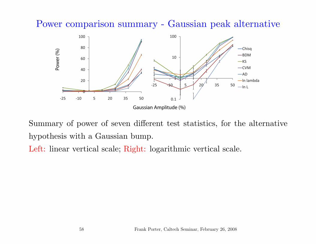
Summary of power of seven different test statistics, for the alternative

hypothesis with a Gaussian bump.

Left: linear vertical scale; Right: logarithmic vertical scale.


Power comparison - High statistics

Also look at the performance for histograms with large bin contents.

Estimates of power for seven different test statistics, as a function of

H1. The comparison histogram (H0) is generated with all k = 100 bins

Poisson of mean 100. The selection is at the 99% confidence level.H0 5 -5

Statistic % % %χ2 0.91 ± 0.23 79.9 ± 1.0 92.1 ± 0.7

BDM 0.97 ± 0.24 80.1 ± 1.0 92.2 ± 0.7

KS 1.03 ± 0.25 77.3 ± 1.0 77.6 ± 1.0

CVM 0.91 ± 0.23 69.0 ± 1.1 62.4 ± 1.2

AD 0.91 ± 0.23 67.5 ± 1.2 57.8 ± 1.2

lnλ 0.91 ± 0.23 79.9 ± 1.0 92.1 ± 0.7

lnL 0.97 ± 0.24 79.9 ± 1.0 91.9 ± 0.7


Comments on power comparison - High statistics

In this large-statistics case, for the χ2 and similar tests, the power to

for a dip is greater than the power for a bump of the same area.

– Presumably because the “error estimates” for the χ2 are based

on the square root of the observed counts, and hence give smaller

errors for smaller bin contents.

Also observe that the comparative strength of the KS, CVM, and AD

tests versus the χ2, BDM, lnλ, and lnL tests in the small statistics

situation is largely reversed in the large statistics case.


Power study for a “sawtooth” alternative

To see what happens for a radically different alternative distribution,

consider sampling from the “sawtooth” distribution. Compare once

again to sampling from the uniform histogram.

The “percentage” sawtooth here is the fraction of the null hypothe-

sis mean. A 100% sawtooth on a 1 count/bin background oscillates

between a mean of 0 counts/bin and 2 counts/bin.

The period of the sawtooth is always two bins.

0 20 40 60 80 100

0.0

0.5

1.0

1.5

2.0

Bin number

H0

or H

1 m

ean

0 20 40 60 80 100

0.0

0.5

1.0

1.5

2.0

0 20 40 60 80 100

01

23

45

Bin number

Cou

nts/

bin

0 20 40 60 80 100

01

23

45

Left: The mean bin contents

for a 50% sawtooth on a back-

ground of 1 count/bin (blue),

and for the flat background (red).

Right: A sampling from the 50%

sawtooth (blue) and from the

uniform background (red).61 Frank Porter, Caltech Seminar, February 26, 2008

Sawtooth alternative power results

Estimates of power for

seven different test statis-

tics, for a “sawtooth” al-

ternative distribution.

50 100Statistic % %χ2 3.7 ± 0.5 47.8 ± 1.2

BDM 1.9 ± 0.3 33.6 ± 1.2

KS 0.85 ± 0.23 1.0 ± 0.2

CVM 0.91 ± 0.23 1.0 ± 0.2

AD 0.91 ± 0.23 1.2 ± 0.3

lnλ 4.5 ± 0.5 49.6 ± 1.2

lnL 0.30 ± 0.14 10.0 ± 0.7

Now the χ2 and lnλ tests are the clear winners, with BDM next.

The KS, CVM, and AD tests reject the null hypothesis with the same

probability as for sampling from a true null distribution. This very

poor performance for these tests is readily understood, as these tests

are all based on the cumulative distributions, which smooth out local

oscillations.


Conclusions

These studies provide some lessons in “goodness-of-fit” testing:

1. No single “best” test for all applications. The statement “test X is bet-

ter than test Y” is empty without more context. E.g., the Anderson-

Darling test is very powerful in testing normality of data against al-

ternatives with non-normal tails (eg, a Cauchy distribution)*. It is

not always especially powerful in other situations. The more we know

about what we wish to test, the better we can choose a powerful test.

Each of the tests here may be useful, depending on the circumstance.

2. Even the controversial L test works as well as the others sometimes.

However, there is no known situation where it performs better than

all of the others, and the situations where it is observed to perform as

well are here limited to those where it is equivalent to another test.

* M. A. Stephens, Jour. Amer. Stat. Assoc. 69 (1974) 730.


Conclusions (continued)

3. Computing probabilities via simulations is a useful technique. How-

ever, must be done with care. Tests with an incompletely specified

null hypothesis require care. Generating a distribution according to

an assumed null distribution can lead to badly wrong results. It is

important to verify the validity of the procedure. We have only looked

into tails at the 1% level. Validity must be checked to whatever level

of probability is needed. Should not assume that results at the 1%

level will still be true at, say, the 0.1% level.

4. Concentrated on the question of comparing two histograms. However,

considerations apply more generally, to testing whether two datasets

are consistent with being drawn from the same distribution, and to

testing whether a dataset is consistent with a predicted distribution.

The KS, CVM, AD, lnL, and L tests may all be constructed for these

other situations (as well as the χ2 and BDM, if we bin the data).64 Frank Porter, Caltech Seminar, February 26, 2008

ASIDESignificance/GOF: Counting Degrees of Freedom

The following situation arises with some frequency (with variations):

I do two fits to the same dataset (say a histogram with N bins):

Fit A has nA parameters, with χ2A [or perhaps −2 lnLA].

Fit B has a subset nB of the parameters in fit A, with χ2B, where the

nA − nB other parameters (call them θ) are fixed at zero.

What is the distribution of χ2B − χ2

A?

Luc Demortier in:

http://phystat-lhc.web.cern.ch/phystat-lhc/program.html


Counting Degrees of Freedom (continued)

In the asymptotic limit (that is, as long as the normal sampling distri-

bution is a valid approximation),

Δχ2 ≡ χ2B − χ2

A

is the same as a likelihood ratio (−2 lnλ) statistic for the test:

H0 : θ = 0 against H1 : some θ = 0

Δχ2 is distributed according to a χ2(NDOF = nA − nB) distribution as

long as:

Parameter estimates in λ are consistent (converge to the correct val-

ues) under H0.

Parameter values in the null hypothesis are interior points of the main-

tained hypothesis (union of H0 and H1).

There are no additional nuisance parameters under the alternative

hypothesis.


Counting Degrees of Freedom (continued)

A commonly-encountered situation often violates these requirements:

We compare fits with and without a signal component to estimate sig-

nificance of the signal.

If the signal fit has, e.g., a parameter for mass, this constitutes an

additional nuisance parameter under the alternative hypothesis.

If the fit for signal constrains the yield to be non-negative, this violates

the interior point requirement.

Freq

uenc

y

0 2 4 6 8 10 12

040

0080

0012

000

2Δχ (H0-H1)

H0: Fit with no signalH1: Float signal yield

Curve: χ2 (1 dof )

Freq

uenc

y

0 2 4 6 8 10 12

050

0015

000

2500

0

2Δχ (H0-H1)

H0: Fit with no signalH1: Float signal yield, constrained 0

_>

Curve: χ2 (1 dof )

Freq

uenc

y0 2 4 6 8 10 12

010

0030

0050

00

H0: Fit with no signalH1: Float signal yield and location

Blue: χ2 (1 dof )

2Δχ (H0-H1)

χ2 (2 dof )Red:


Counting Degrees of Freedom - Sample fits50

080

0

H0 fit H1 fit

Fix meanAny signal

0 40 80

500

800

x

Cou

nts/

bin

H1 fit

Fix meanSignal>=0

0 40 80x

H1 fit

Float meanAny signal

500

800

H0 fit H1 fit

Fix meanAny signal

0 40 80

500

800

x

Cou

nts/

bin

H1 fit

Fix meanSignal>=0

0 40 80x

H1 fit

Float meanAny signal

Fits to data with no signal. Fits to data with a signal.


Documents

Goodness-of-Fit â€“ Pitfalls and Power Example: Testing Consistency of Two Histograms