Embed Size (px)
Citation preview

RTG 1666 GlobalFood ⋅ Heinrich Düker Weg 12 ⋅ 37073 Göttingen ⋅ Germany www.uni-goettingen.de/globalfood
ISSN (2192-3248)
www.uni-goettingen.de/globalfood
RTG 1666 GlobalFood
Transformation of Global Agri-Food Systems: Trends, Driving Forces, and Implications for Developing Countries
Georg-August-University of Göttingen
GlobalFood Discussion Papers
No. 76
Mobile money and household food security in Uganda
Conrad Murendo
Meike Wollni
January 2016

1
Mobile money and household food security in Uganda
Conrad Murendoa* and Meike Wollnia
aDepartment of Agricultural Economics and Rural Development, Georg-August-University of
Goettingen, 37073 Goettingen, Germany
* Corresponding author; phone: +49-551-3920212, fax: +49-551-3920203,
e-mail: [email protected]
Abstract.
Despite the fact that the use of mobile money technology has been spreading rapidly in developing
countries, empirical studies on the broader welfare effects of the technology on rural households
are still limited. Using household survey data, we analyse the effect of mobile money on household
food security in Uganda. Unlike previous studies that rely on a single measure of food security, we
measure food security using two indicators – a food insecurity index and food expenditures. To
account for selection bias in mobile money use, we estimate treatment effects and instrumental
variables regressions. Our results indicate that the use of mobile money per se as well as the
volumes transferred are associated with a reduction in food insecurity. Furthermore, the use,
frequency of use, and volumes of mobile money transferred are associated with increases in food
expenditures. Policy interventions and strategies aiming to improve household food security should
consider the promotion of mobile money among rural households in Uganda and other developing
countries as a promising instrument.
Keywords: mobile money; food security; households; Uganda
JEL codes – G29, I31, O16, O33
Acknowledgement
The authors acknowledge financial support from German Research Foundation (DFG) and German
Academic Exchange Service (DAAD). We are also grateful to Grameen Foundation for support in
fieldwork coordination. The authors take responsibility for all remaining errors.

2
1. Introduction
Mobile money, the use of mobile phones to perform financial and banking functions, is spreading
rapidly in developing countries (Donovan, 2012; IFC, 2011). Mobile money offers various benefits,
which are especially useful in developing countries where financial access is limited (Donovan,
2012; Kikulwe et al., 2014). One key benefit is improving access to financial services for the poor
and those with no formal bank accounts. Mobile money facilitates financial transactions through
affordable payment systems, which is of particular importance in developing countries where
households rely on remittances from family members (Donovan, 2012; IFC, 2011; Jack et al.,
2013). The affordability of mobile money also emanates from modest and proportionate withdrawal
fees, which are usually not a barrier to poor households transacting in small amounts. Other benefits
are associated with reduced security risk of moving around with cash and faster transfer of money
into rural areas (Kikulwe et al., 2014). Savings and insurance products are also now being offered
through mobile money. This is particularly valuable for poor households as it offers the possibility
for protection against vulnerabilities such as illness and to smooth consumption (Jack and Suri,
2014).
A growing number of studies document the positive effect of financial access on savings behaviour
(Karlan et al., 2014), consumption, and productive investment (Adams and Cuecuecha, 2013;
Dupas and Robinson, 2013). Mobile money is an innovation that has the potential to improve
financial access especially for rural households with no access to formal bank accounts. Rural
households could gain from using mobile money through faster transfer of money from various
sources (e.g. remittances, payment from traders, wage etc), lower financial transaction costs and
availability of other financial instruments for example savings and insurance. Mobile money is
expected to bridge the financial access gap, thus allowing for food security and broader welfare
improvements especially among the financially excluded rural communities in developing
countries. To date there are only few studies that have analysed the welfare effects of mobile money
3
on rural households in developing countries (Jack et al., 2013; Jack and Suri, 2014; Kikulwe et al.,
2014; Munyegera and Matsumoto, 2014). Most of these studies find positive effects of mobile
money on household income (Kikulwe et al., 2014), consumption smoothing (Jack and Suri, 2014)
and per capita consumption (Munyegera and Matsumoto, 2014).
The above-mentioned studies provide important empirical evidence of the broader welfare effects
of mobile money. However, little is known about the effects of mobile money on food security of
the rural poor. This article fills this gap by analysing the effect of mobile money on household food
security in Uganda, where the use of mobile money has grown rapidly in recent years. Our paper
contributes to the emerging literature on mobile money in several ways. First, to the best of our
knowledge this is the first paper that analyses the effects of mobile money on food security in a
developing country context. Second, unlike studies that use one measure of food security, we take
the multidimensional nature of food security into account (Maxwell et al., 2014) and use two
distinct measures. In addition to food expenditures (an objective and monetary measure), we use a
subjective and non-monetary measure: the Household Food Insecurity Access Scale (HFIAS). The
advantage of the HFIAS is that it includes many facets of food security and also captures
subjectively perceived risks of food insecurity. In addition, measurement errors are minimal, in
particular in comparison to consumption indicators (Kabunga et al., 2014). The use of two distinct
and complementary measures allows us to address the robustness of our results to choosing
different outcome variables. Our study is also unique in that we use alternative specifications of
the treatment variable; namely mobile money use, frequency of use and volumes transferred via
mobile money services.
The remainder of this article is organised as follows. In the next section we describe the conceptual
framework. Section three presents the methodology, including the description of survey data and
food security measures used in the empirical analysis. Section four describes the estimation strategy

4
employed. Empirical results are presented and discussed in section five and the last section
concludes and derives policy implications.
2. Conceptual framework
In our framework, we follow Munyegera and Matsumoto (2014) and consider the same rural
household in two scenarios: with and without the introduction of mobile money (Figure 1). The
rural household is located in a remote village where financial institutions are not available. This
household receives money from various sources (e.g. remittances, payments from traders, wages
or pensions) in both scenarios. The only difference is the money transfer or payment method, which
affects the overall disposable income. In scenario one, cash is transferred physically through slow
and insecure informal methods (e.g by person, bus, taxi) between the sender working in an urban
area and the receiver in the rural village (Kikulwe et al., 2014; Munyegera and Matsumoto, 2014).
In addition, household members have to travel to distant business centres to receive payments for
their agricultural produce from traders as well as access other financial services, for example their
pension. This is associated with high costs of accessing capital both in terms of the transport fare
and the opportunity cost of travel time between the two locations. The high transaction costs reduce
household disposable income and investment in food, health, education and agricultural inputs.
Consequently, overall household welfare is reduced.

5
Figure 1. Pathways through which mobile money may affect household food security
In scenario two, mobile money is introduced facilitating access of rural households in remote areas
to monetary transfers, such as remittances, payments and pensions. In scenario two, we will likely
observe an increased flow of cash into rural households because of the introduction of a relatively
faster and safer financial service innovation. The benefits realized through using mobile money
have the potential to contribute to household disposable income and food security through at least
three pathways. First, the household is able to receive cash faster and more immediately from
various sources (e.g. remittances, payments from traders, wages or pension payments). This will
result in greater liquidity, which can be used for household productive and consumptive purposes
(Adams and Cuecuecha, 2013).
Receive cash from various sources (e.g.
remittances, traders, wage, salary etc)
Faster cash flow and liquidity
Lower transaction costs - time and travel
Access to other services (e.g. savings,
insurance) improved
Higher disposable income
Increased investment in food, health,
education, agricultural inputs, savings
Improved food security and welfare
Scenario two
With mobile money
Rural household in
remote village
Scenario one
No mobile money
Co
nd
ition
s
Mech
an
isms
O
utco
me
Receive cash from various sources (e.g.
remittances, traders, wage, salary etc)
Slow cash flow and liquidity
Higher transaction costs - time and travel
Access to other services (e.g. savings,
insurance) constrained
Lower disposable income
Decreased investment in food, health,
education, agricultural inputs, savings
Reduced food security and welfare

6
The second pathway through which mobile money can affect household welfare and poverty is
through lower transaction costs. Mobile money can be an accessible, convenient and cheap medium
for the delivery of financial services and more reliable than traditional and informal methods
(Kikulwe et al., 2014). In many countries, mobile money is a relatively cheaper means of money
transfer than other alternatives (Donovan, 2012) and users benefit from the reduced time and
monetary costs of accessing financial services. The lower transaction costs associated with sending
money via mobile money services can directly translate into more money available to households
for various consumption expenditures, including food, health, and education, as well as productive
investment in agriculture or alternative income-generating activities.
Third, it is now possible to extend the range of financial services offered by mobile money beyond
basic payment and withdrawal to other financial products, for example savings and insurance (IFC,
2011). With access to savings or insurance services, households can efficiently manage risks and
invest in improving agricultural production.
Some evidence in support of these impact pathways can be found in the literature. Jack et al. (2013)
show for example that the introduction of mobile money positively increased the volumes of
internal remittances in Kenya. Similarly, Kikulwe et al. (2014) and Munyegera and Matsumoto
(2014) show that mobile money is associated with higher remittances received by households. Jack
and Suri (2014) found that remittances received via mobile money enabled households in Kenya
to smooth consumption, thus offering a form of risk insurance. In this section, we discussed that
mobile money potentially lowers the transaction and opportunity costs of transferring money and
enhances liquidity through faster transfer of cash. Through these pathways, we therefore
hypothesize that mobile money improves food security and welfare among rural households.

7
3. Methodology
3.1. Data
This article uses data collected from rural households in Mukono and Kasese districts in Uganda.
We applied a multi-stage approach to draw the sample. In the first stage, we randomly selected
approximately 20 villages in each of the two districts. In the second stage, we randomly selected
about 12 households in each village for the interviews. Households were chosen from lists that
were compiled in collaboration with the village administration, NGO workers and local extension
staff. In total, we interviewed 482 households in 39 villages. For the analysis, we had to drop six
households because of inconsistent data on consumption and expenditures. The survey instrument
contained a mobile money module, based on which we can distinguish between households using
mobile money services and those who are not. Our analysis is based on 273 mobile money users
and 203 non-users as shown in Table 1.
Table 1. Sample differentiated by mobile money adoption status
Non-Adopters Adopters Total
Mukono 92 147 239
Kasese 111 126 237
Total 203 273 476
The data were collected through personal interviews using a pre-tested questionnaire during
November and December 2013. The questionnaires were administered to the household head
and/or the spouse. Data on socioeconomic characteristics, including food consumption and
expenditures, were collected at the household level. Details on food consumption were collected
using a 7-day recall period for food, beverages and tobacco. A 30-day recall period was used to
capture purchases of more durable goods and services that are undertaken by households less
frequently (Deaton and Zaidi, 2002). The HFIAS module consisted of nine questions, representing
different experiences of food insecurity over the last 30 days (Coates et al., 2007).

8
A household is defined as a mobile money user if any member of the household used mobile money
services in the past 12 months prior to the survey (Kikulwe et al., 2014). We measure the frequency
of using mobile money as the number of times a household sent or received money via mobile
phone in the past 12 months, with zero values indicating that mobile money has not been used. This
is similar to the approach used by Kirui et al. (2012). The volume of mobile money transferred is
measured as the sum of money sent and received during the past twelve months, with zero values
indicating that no money has been transferred through mobile phones.
3.2. Food security measurement
According to the World Food Summit in 1996, food security exists when all people, at all times,
have physical and economic access to sufficient safe and nutritious food to meet their dietary needs
and food preferences for a healthy and active life (FAO, 1996). Food security is multidimensional
and this makes its measurement particularly complex. Several indicators have been used to measure
food security. Barrett (2010) gives an overview of objective measures of food security, e.g. dietary
intake, expenditures, and health indicators, as well as subjective measures, e.g. perceived adequacy
of consumption, exposure to risk, and the cultural acceptability of foods. A drawback of most of
the approaches based on dietary intake and anthropometric indicators is that they are expensive and
data intensive (de Haen et al., 2011). Maxwell et al. (2014) provide a review of subjective indicators
commonly used by agencies working on food security, such as the World Food Program. These
include: a) dietary diversity and food frequency, e.g. Household Dietary Diversity Score and Food
Consumption Score; b) consumption behaviours, e.g. Coping Strategies Index; c) experiential
measures, e.g. the Household Food Insecurity Access Scale and the Household Hunger Scale; and
d) self-assessment measures. These subjective measures are simple and easy to use, but their main
disadvantage is that they focus only on measuring food access and do not account for food intake
and availability. Maxwell et al. (2014) highlight that food security is a multidimensional livelihood
outcome and thus should ideally be measured by multiple indicators. In this paper, we use food
9
expenditures as an objective measure and the Household Food Insecurity Access Scale (HFIAS) as
a subjective measure of food security. We describe each of these measures separately in the next
subsections.
3.2.1. Food Expenditure
We used a 7-day recall period to elicit expenditures on food, beverages and tobacco and a 30-day
recall period in the case of household expenditures on less frequently purchased food items. We
collected expenditure data on an item-by-item basis. Conversion factors were used to change food
consumption expenditures to a 30-day monthly basis. Subsequently, all expenditures were
aggregated to derive total food consumption expenditures at household level. Consumption of
home-produced food was valued at local market prices. Finally, per capita food consumption
expenditures were calculated based on monthly per adult equivalents (AE). We use the OECD adult
equivalent scale which is given by: 1 + 0.7(A − 1) + 0.5C, where A and C represent the number
of adults and children in a household, respectively (Deaton and Zaidi, 2002). For the econometric
analysis, the monthly food expenditure per AE was normalized by log transformation.
3.2.2. Household Food Insecurity Access Scale (HFIAS)
The HFIAS measures the degree of food (access) insecurity (Coates et al., 2007). According to
Coates et al. (2007) and Maxwell et al. (2014), the HFIAS is a simple, cost effective and
scientifically valid indicator, which captures household experiences in terms of insufficient quality,
quantity and uncertainty over insecure food access. The HFIAS is widely used in international
contexts and its recent applications to Sub-Saharan Africa include Cock et al. (2013) for South
Africa, Kabunga et al. (2014) and Keino et al. (2014) for Kenya, and Maxwell et al. (2014) for
Ethiopia.
The HFIAS consists of asking household heads to respond to nine questions, which represent
universal domains of the experience of insecure access to food. The nine questions (sub-domains)
10
are grouped into three main domains (Coates et al., 2007; Cock et al., 2013; Kabunga et al., 2014;
Keino et al., 2014). The details of the domains and sub-domains are shown in Table 2. Domain I
represents anxiety and uncertainty about household food supply. Domain II represents insufficient
food quality, while domain III represents insufficient food quantity intake and physical
consequences. Respondents answered each sub-domain using a score from 0 to 3, depending on
whether the particular problem described occurred: never (non-occurrence), rarely (1–2 times),
sometimes (3–10 times), or often (more than 10 times) over the last 30 days. For each individual
household, the HFIAS score is computed by aggregating the sub-domain scores, and ranges from
0 to 27. The higher the score, the greater the food insecurity the household experienced; whereas a
lower score represents a more food-secure household (Coates et al., 2007).
3.2.2.1. Food insecurity index (FIN)
Creating the dependent variable by summing up the HFIAS scores (Cock et al., 2013; Keino et al.,
2014) has the disadvantage of assigning equal weight to each item, regardless of its value or utility.
For impact analysis this may not be informative because the sub-domains capture different aspects
of food insecurity (Kabunga et al., 2014). One approach to address this weakness involves using
factor analysis to create composite scores that capture the common patterns in the data (Kabunga
et al., 2014). We therefore created a Food Insecurity Index (FIN) based on the HFIAS using weights
obtained from the factor analysis. Kabunga et al. (2014) highlight that the food insecurity index
computed from factor analysis represents relative food insecurity within the sample and is suitable
for impact evaluations because it compares the extent to which one household differs from the
other. Factor analysis determines and assigns weights to capture the relative importance of multiple
indicators and maximize the variance explained by the linear composites. The use of factor analysis
in this context is a well-established method that has been applied in numerous studies (McKenzie,
2005; Sahn and Stifel, 2000).

11
In this study, factor analysis was applied to the nine sub-domains of the HFIAS to determine the
combination yielding the best accuracy performance for the FIN. In our analysis, eight subdomains
loaded highly on the first principal factor. The first factor, which explains 77% of the variation, is
considered our measure of food insecurity (Sahn and Stifel, 2000). The factor loadings are shown
in Table 2. Positive factor loadings indicate a positive correlation of the variable with relative food
insecurity and vice versa. Higher values of the index reflect higher levels of food insecurity.
The appropriateness of the application of factor analysis to our data was confirmed by the Kaiser-
Meyer-Olkin (KMO) measure of sampling adequacy and Bartlett test of sphericity. The KMO
yielded a value of 0.85 and Field (2013) recommends accepting KMO values above 0.6. The
Bartlett test of sphericity tests the null hypothesis that the original correlation matrix is an identity
matrix. The Bartlett test yielded 𝜒2 = 2896.03 (p = 0.000); hence, we reject the null hypothesis and
conclude that there are significant relationships between the variables used for the index. While the
KMO and Bartlett test indicate the data’s adequacy for factor analysis, the scale reliability is
expressed via the Cronbach’s alpha statistic. The corresponding statistic of 0.88 shows that the
scale reaches the advisable minimum of 0.7 and therefore consistently reflects the construct that it
is measuring (Field, 2013; Keino et al., 2014). The scale’s consistency was assessed by correlating
the individual sub-domains with the total scale score. The sub-domains are highly correlated with
the total score, a reflection of internal consistency.
3.2.2.2. Binary food insecurity
We also used a binary food insecurity indicator as an alternative to the food insecurity index. This
approach allows us to define discrete food insecurity levels. To determine the cut-off for these food
insecurity levels, we used the Household Food Insecurity Access Prevalence (HFIAP) developed
by Coates et al. (2007), which uses the same questions as the HFIAS to categorize households into
four levels of food insecurity. The four categories of food insecurity are: 1 = food secure, 2 = mildly
food insecure, 3 = moderately food insecure and 4 = severely food insecure. Households are

12
categorized as increasingly food insecure as they respond affirmatively to more severe conditions
and/or experience those conditions more frequently (Coates et al., 2007). In our analysis, we merge
categories 1 and 2 into food-secure households, and categories 3 and 4 into food-insecure
households (Kassie et al., 2014b).
4. Estimation strategy
As discussed in the conceptual framework, mobile money is expected to have positive effects on
food security. Econometrically, we examine the effect of mobile money on food security using the
following specification:
𝐹𝑆 = 𝛽𝑿 + 𝛿𝑀𝑀 + 휀 (1)
Where 𝐹𝑆 is one of the food security related outcome variables (food expenditures, food insecurity
index, and binary food insecurity); 𝑿 is a vector of regressors influencing the outcome variable;
and 𝑀𝑀 is the treatment variable (specified as dummy variable for the use of mobile money
services, or as continuous variable in the case of frequency of use or volume transferred).
Furthermore, 𝛽 is a vector of parameters to be estimated, and 𝛿, which is also estimated by the
model, measures the effect of mobile money on food (in-) security. Finally, 휀 is an i.i.d. random
error term.
When analysing food security, mobile money might be subject to selection bias resulting from
unobservable factors influencing not only household’s use of mobile money services, but also their
food security. For example, mobile money users may be more technically literate and more likely
to have family members in the capital city or abroad sending remittances. As a result, mobile money
users are more likely to have higher average levels of income and human capital and consequently
lower average levels of food insecurity. Due to such potential selection bias, mobile money users
and non-users are not directly comparable, which implies that an estimation method needs to be
chosen that corrects for this bias in order to obtain unbiased estimates of the effect of mobile money

13
on food security. We therefore use endogenous treatment effects models (in the case of binary
treatment variable specification) and instrumental variables regressions (in the case of continuous
treatment variable specification) to control for observed and unobserved heterogeneity when
estimating the effect of mobile money on food expenditure and food insecurity.
In this study, we use two different instruments: household-specific mobile phone network
connectivity and the size of the information exchange network of the household. Regarding mobile
phone network connectivity, we asked the household how many network bars are displayed on the
mobile phone at the homestead ranging from 0 to 4 (0 equals no network and 4 excellent network
connectivity). We classified 0 to 2 network bars into “poor network connectivity” and 3 to 4
network bars into “good network connectivity”. While in principle poor network connectivity at
home can be overcome by using network services elsewhere, we expect a positive correlation
between network availability at home and the (frequency and extent of) use of mobile phone based
financial services. The second instrument – the size of the information exchange network – is based
on social network data that was obtained using random matching within sample (Maertens and
Barrett, 2013). For this purpose, each interviewed household was matched with five other
households randomly drawn from the sample. Conditional on knowing the matched household, the
interviewee was asked whether they have ever talked about mobile money. Based on this data, our
instrument contains the number of matched households with which information on mobile money
services has been exchanged. It is thus a measure for information access and accordingly
hypothesized to be positively correlated with the household’s use of mobile money services. While
both instruments are strongly correlated with mobile money use, they are unlikely to affect
household food security directly. Beyond the instruments described here, we tested other potential
instruments, for example, the proportion of households using mobile money and owning a mobile
phone in the village (Kikulwe et al., 2014). However, these variables did not qualify as good
instruments in our case study.

14
The choice of the control variables used in the estimations is guided by the emerging literature on
mobile money use (Jack and Suri, 2014; Kikulwe et al., 2014; Kirui et al., 2013) and the broader
literature on technology adoption and food security (Kabunga et al., 2014; Kassie et al., 2014b;
Shiferaw et al., 2014). All variables are described in Table 3 below. Besides household
demographic and socio-economic control variables, we included a number of variables related to
information access. Firstly, we include the variable "number of mobile phones owned" as a proxy
for information access. Controlling for the number of mobile phones owned also allows us to make
sure that our variable of interest "mobile money" is not confounded with other more general
benefits of mobile phone ownership. Secondly, we included the variable "extension contact"
measuring whether a household had accessed information from extension service. In particular, in
the research area an extension program had been implemented that uses locally recruited farmers
known as community knowledge workers to disseminate mobile-phone based extension.
Community knowledge workers are trained by an NGO to use smart phones to access agricultural
and market information and provide this information to fellow farmers in their respective villages.
Thirdly, we include the variable "group membership" as a proxy for access to information. In
general, improved access to agricultural and market information is expected to improve agricultural
productivity, incomes, and thus food security.
5. Results and discussion
5.1. Use of mobile money
Overall, 57% of the households in the sample use mobile money. On the average, mobile money
was used seven times during the past 12 months, ranging from a minimum of one to a maximum
of ten times. Figure 2 shows the activities for which households use mobile money services. Around
96% of the mobile money users stated that they withdraw money from their mobile account. This
money may come from various sources (e.g. remittances or payments from traders) and is used for
a variety of household activities – for example purchases of food or agricultural inputs among

15
others. Fifty seven percent of the mobile money users stated that they use their mobile money
accounts as savings account. About 53% of the households stated that they also transfer money to
relatives and friends, and 25% of the households use mobile money to buy airtime for their mobile
phones. Eighteen percent used mobile services to transfer money to business partners and a similar
proportion (18%) used mobile services to pay school fees.
Figure 2. Activities performed with mobile money services
5.2. Results of descriptive analysis
The sample statistics for the HFIAS sub-domains are shown in Table 2. The proportion of
households responding ‘never’ in the first sub-domain is about 48%, implying that 52% of the
sampled households were anxious and uncertain about their food supply. In domain II, the average
proportion of ‘never’ responses is 35%. This means that roughly 65% of the households have
insufficient food quality. Lastly, in domain III, the average proportion of ‘never’ responses is 79%,
implying that about 21% have insufficient food quantity intake due to physical unavailability.
0 10 20 30 40 50 60 70 80 90 100
Withdraw money
Save money
Transfer money to relatives and friends
Buy airtime
Transfer money to business partners
Pay school fees
Pay bills
Transfer money to own account
Percent of mobile money users

16
Table 2. Sample statistics for the HFIAS sub-domains (Percentage response on occurrences in the last 30 days)
Never
(0
times)
Rarely
(1-2
times)
Sometimes
(3-10 times)
Often
(>10
times)
Factor
loadings
Domain I. Anxiety and uncertainty about household food
supply
1. Did you worry that your household would not have enough
food? (Anxiety)
47.90 16.39 27.10 8.61 0.778
Domain II. Insufficient quality (includes food variety and
preferences)
2. Were you or any household member not able to eat the
kinds of foods you preferred because of a lack of resources?
(Kinds)
34.66 12.18 38.87 14.29 0.825
3. Did you or any household member have to eat a limited
variety of foods due to a lack of resources? (Variety)
37.61 11.76 36.76 13.87 0.817
4. Did you or any household member have to eat some foods
that you really did not want to eat because of a lack of
resources to obtain other types of food? (Not want)
33.61 12.61 39.08 14.71 0.779
Domain III. Insufficient food intake and physical
consequences
5. Did you or any household member have to eat a smaller
meal than you felt you needed because there was not enough
food? (Smaller)
57.37 10.71 27.52 4.41 0.786
6. Did you or any household member have to eat fewer meals
in a day because there was not enough food? (Fewer)
61.34 7.98 25.63 5.04 0.767
7. Was there ever no food to eat of any kind in your household
because of a lack of resources to get food? (No Food)
86.76 3.15 9.03 1.05 0.525
8. Did you or any household member go to sleep at night
hungry because there was not enough food? (Sleep)
92.02 2.31 5.46 0.21 0.465
9. Did you or any household member go a whole day and
night without eating anything because there was not enough
food? (Whole day)
95.80 2.31 1.89 0.00 0.306

17
Figure 3 shows the food insecurity categories based on the HFIAP classification. The proportions
of food secure and mildly food insecure households are higher among mobile money users, while
the proportions of moderately and severely food-insecure households are higher among non-users.
Figure 3. Food insecurity categories
Similarly, mobile money users have an average food insecurity index score of -0.20, which is
significantly lower compared to the index score of 0.27 for non-users. The mean difference of 0.47
is statistically significant at the 1% level based on t-test results. Similarly, the monthly food
expenditure per AE of users (82861 UGX1) is higher than that of non-users (76479 UGX), which
is significant at the 10% level. These results suggest that users are more likely to be food secure
than non-users. While these descriptive differences cannot be interpreted as causal impacts, they
provide an indication that there may be structural differences in food security and expenditures
between mobile money users and non-users. In the following sections, we use econometric
techniques to identify the effect of mobile money.
Table 3 presents the descriptive statistics of potential explanatory variables included in the
econometric models differentiated by mobile money use. For some of these variables, we observe
significant differences between users and non-users. On average, mobile money users have better
1 The exchange rate was 2500 Uganda Shillings (UGX) =1USD at the time of survey.
19.7
34.84.9
8.4
52.2
42.1
23.214.7
0%
10%
20%
30%
40%
50%
60%
70%
80%
90%
100%
Non-Users Users
Severely food insecure
Moderately food insecure
Mildy food insecure
Food secure

18
access to information, as captured by the variables group membership and number of mobile phones
owned.
There are also significant differences with respect to education levels, land holdings and livestock
ownership. Better educated mobile money users and those with larger land holdings are more likely
to have higher agricultural productivity and to be food secure. Users are more likely to be involved
in off-farm income activities, suggesting that household members engaged in off-farm activities
may possibly send remittances using mobile money. Off-farm income activities increase household
cash, which might be used either to purchase sufficient food or invest in agriculture to increase
agricultural productivity and production to meet household food security needs. Earlier studies
show the importance of off-farm income for food security (Mabiso et al., 2014; Sinyolo et al.,
2014). Considering land, assets, off-farm income activity and livestock as proxies for wealth,
results suggest that mobile money users are wealthier than non-users. Significantly more of the
mobile money users also have their own means of transportation. This gives them an advantage in
mobility and access to agricultural input and output markets.

19
Table 3. Differences between mobile money users and non-users
*** indicates the corresponding mean differences are significant at the 1% level (t-tests).
2 TLU is calculated using the numbers of livestock owned by the household using the Storck (1991) conversion factors:
cows, oxen, bulls = 1; heifers = 0.75; calves = 0.25; donkey = 0.5; goat, sheep = 0.1; pig = 0.2; chickens = 0.01.
Users Non-users
Variable Description Mean Std Mean Std
Treatment variables
Frequency Number of times household used mobile money 7.22 2.77 - -
Volume transferred Volume of mobile money transferred (log) 12.16 1.42 - -
Control variables
Group membership Household member(s) belong to any group
(dummy)
0.766*** 0.42 0.606 0.49
Mobile phones Number of mobile phones owned by household 2.018*** 1.06 0.842 0.93
Extension contact Household accessed information from extension
service (dummy)
0.564*** 0.50 0.419 0.50
Age Age of household head (years) 49.377 12.85 49.897 14.48
Gender Gender of household head (dummy, 1=male) 0.897*** 0.30 0.788 0.41
Education Education of household head (years) 7.414*** 4.46 5.064 3.85
Household size Household size (number) 7.326*** 2.64 6.596 2.93
Dependency ratio Ratio of dependents (15 & below, 65 plus) to
workforce (16-64)
1.362 1.10 1.499 1.26
Adult equivalent Adult equivalent 4.603*** 1.51 4.165 1.67
Land size Size of land owned in acres 5.153*** 5.43 3.619 3.25
Ln(Farm equipment) Value of farm equipment (log) 10.943*** 1.26 10.502 1.09
Off farm income Household member(s) engaged in off-farm income
activity (dummy)
0.619*** 0.49 0.355 0.48
Access to credit Household accessed credit (dummy) 0.546*** 0.50 0.345 0.48
TLU Total livestock units2 1.242*** 2.21 0.671 1.50
Means of transport Household owns motorcycle and/or car (dummy) 0.201*** 0.40 0.059 0.24
Output market Distance to output market (km) 3.758 4.69 4.252 6.52
District Household is located in Mukono district (dummy) 0.538 0.50 0.453 0.50
Instruments
Size of exchange
social network
Number of network members household
communicates with about mobile money
0.498*** 1.13 0.089 0.39
Connectivity Mobile phone network connectivity (dummy,
1=good connectivity, 0=poor connectivity)
0.780*** 0.41 0.507 0.50
Observations 273 203

20
5.3. Econometric results
In this section, we present the econometric results of the effects of mobile money use on food
security. As described above, we measure food security using the food insecurity index, binary
food insecurity, and food expenditure. The effects of mobile money on these outcome variables are
discussed separately in the next sub-sections.
5.3.1. Effect of mobile money on food expenditure
The results from the endogenous treatment effects model on the effect of mobile money use on
food expenditure are shown in column 2 of Table 4. The size of the exchange social network and
mobile phone network connectivity are used as instruments in the endogenous treatment effects
model. The Wald test of independent equations is insignificant, indicating that there is no selection
on unobservables. We therefore rely on OLS regression for estimation. The results of the OLS
model show that mobile money use is positive and significant at the 10% level. The estimated
coefficient indicates that the adoption of mobile money leads to a nine-percentage point increase
in monthly food expenditure per adult equivalent.
A number of other covariates are significant. The number of mobile phones owned by the
household has a negative and significant effect on food expenditure per AE. Households having
many mobile phones may incur higher costs associated with airtime, charging costs, repair and
maintenance, which may reduce the food expenditure budget. Furthermore, larger households are
associated with lower levels of food expenditures per adult equivalent. An additional member in
the household reduces food expenditure per adult equivalent by 4.4 percentage points. This estimate
is in line with results based on per capita food consumption reported by Shiferaw et al. (2014). The
variables land size, value of farm equipment, and TLU are positive and highly significant. An
additional acre of land results in 0.7 percentage points increase in food consumption per AE. A one
percent increase in the value of farm equipment is associated with a 5-percentage point increase in
21
food expenditure per AE. An increase in TLU by one unit increases food consumption by 2.3
percentage points. Again, these results are in line with Shiferaw et al. (2014) who found for the
case of Ethiopia that livestock ownership increases per capita consumption expenditure. Finally,
owning a means of transport has a positive effect that is significant at the 10% level.
Table 4 also presents the results for the alternative specifications of the treatment variable: column
6 shows the estimated treatment effects of the frequency of using mobile money; column 8 shows
the estimated treatment effects of the volumes transferred through mobile money. For both
specifications, we first estimated IV regressions. The Hausman (endogeneity) test reported at the
bottom of the table is insignificant for both specifications highlighting absence of selection bias.
We therefore interpret the results of the OLS estimations. The OLS results reveal that the frequency
of using mobile money has a significant effect on food expenditures. If the number of times mobile
money is used is increased by one, food expenditures per AE increase by 1.9 percentage points.
Similarly, the volumes transferred through mobile money are positively and significantly
associated with food expenditures. A one-percentage point increase in the volumes transferred
increases food expenditure per AE by 1 percentage point. The signs and magnitudes of the
estimated coefficients of other covariates are consistent across the different model specifications.

22
Table 4. Estimated effects of mobile money on monthly food expenditure per AE (log) (n= 476)
Dependent variable: food expenditure per AE Use (dummy) Frequency Volume transferred
Treatment effects OLS IV OLS IV OLS
Coeff SE‡ Coeff SE‡ Coeff SE Coeff SE‡ Coeff SE Coeff SE‡
Mobile money 0.225* 0.125 0.091* 0.048 0.057 0.036 0.019*** 0.006 0.034* 0.020 0.010*** 0.004
Extension contact 0.027 0.042 0.026 0.042 -0.021 0.054 0.014 0.043 0.002 0.046 0.023 0.042
Group membership 0.053 0.052 0.054 0.053 0.058 0.052 0.058 0.053 0.044 0.053 0.053 0.053
Mobile phones -0.041* 0.021 -0.036* 0.021 -0.095* 0.051 -0.046** 0.021 -0.087** 0.044 -0.041** 0.021
Age 0.001 0.002 0.001 0.002 0.002 0.002 0.002 0.002 0.001 0.002 0.001 0.002
Gender 0.029 0.063 0.025 0.064 0.016 0.063 0.027 0.064 -0.002 0.065 0.022 0.064
Education 0.007 0.005 0.008 0.005 -0.001 0.008 0.005 0.005 0.005 0.006 0.008 0.005
Household size -0.044*** 0.008 -0.044*** 0.009 -0.042*** 0.009 -0.044*** 0.009 -0.043*** 0.009 -0.044*** 0.009
Dependency ratio 0.025 0.017 0.025 0.018 0.031 0.020 0.026 0.018 0.032 0.020 0.026 0.018
Land size 0.007* 0.004 0.007* 0.004 0.003 0.006 0.006 0.004 0.005 0.005 0.007 0.004
Ln(Farm equipment) 0.049** 0.020 0.050** 0.020 0.039* 0.021 0.046** 0.020 0.043** 0.020 0.048** 0.020
Off farm income -0.012 0.046 -0.011 0.047 -0.047 0.055 -0.014 0.047 -0.060 0.058 -0.017 0.047
Access to credit 0.021 0.044 0.023 0.045 -0.005 0.052 0.019 0.045 -0.011 0.052 0.018 0.045
TLU 0.023** 0.011 0.023** 0.011 0.026** 0.013 0.024** 0.011 0.025** 0.013 0.023** 0.011
Means of transport 0.103* 0.054 0.104* 0.055 0.045 0.078 0.090 0.055 0.071 0.069 0.099* 0.055
Output market 0.005 0.003 0.005 0.004 0.007 0.004 0.005 0.003 0.007 0.004 0.005 0.004
District 0.022 0.052 0.018 0.053 -0.023 0.062 0.014 0.053 -0.038 0.065 0.011 0.052
Constant 10.561*** 0.241 10.636*** 0.237 10.747*** 0.232 10.668*** 0.236 10.707*** 0.224 10.653*** 0.236
𝑎𝑡ℎ(𝜌) -0.201 0.177
Wald test of independent equations (p-value) 0.255
Wald statistic/F statistic 98.90*** 6.02*** 4.388*** 6.36*** 4.39*** 6.17***
Anderson LM statistic 15.17*** 21.90***

23
*, **, *** indicates coefficients are significant at 10%, 5%, and 1% levels. ‡ Robust standard errors are reported. /a Dummy variable used in frequency and volumes specifications. Only second stage
IV estimates are shown.
Cragg-Donald Wald F statistic 7.52 11.02
Sargan statistic(p-value) 0.40 0.69
Endogeneity test (p-value) 0.27 0.20

24
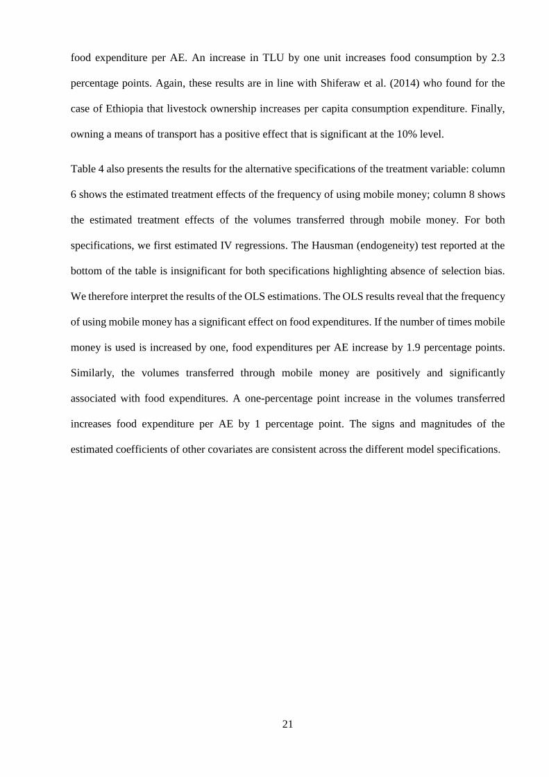
5.3.2. Effect of mobile money on food insecurity
5.3.2.1. Effect of mobile money on the food insecurity index
Table 5 presents the estimation results on the effects of mobile money use, frequency of use, and
volumes transferred on the food insecurity index. To test for potential selection bias, we estimate
an endogenous treatment effects model (in the case of mobile money use) and instrumental
variables regressions (in the case of frequency of use and volumes transferred) using the size of the
exchange social network and mobile phone network connectivity as instruments. In the endogenous
treatment effects model the Wald test of independent equations is statistically significant; we thus
reject the null hypothesis that 𝜌 equals zero. The parameter 𝜌 reflects the correlation between the
error terms of the selection and outcome equations (Miyata et al., 2009; StataCorp, 2013). A
significant 𝜌 indicates that selection bias is present, and thus the endogenous treatment model
results are preferred over the OLS results. Given that our outcome variable is food insecurity, the
positive sign of 𝜌 indicates a negative selection bias, i.e. the OLS estimates presented in column
two of Table 5 underestimate the effect of mobile money on food insecurity. Negative selection
bias in our case implies that households with lower food insecurity scores (i.e. more food secure
households) are more likely to adopt mobile money. This correlation can be a result of unobserved
factors that determine food insecurity and at the same time increase the likelihood of mobile money
use, such as innate ability or motivation.
The results of the endogenous treatment effects model controlling for selection bias are presented
in column four of Table 5. For the interpretation of the results it is important to keep in mind that
the dependent variable is food insecurity; therefore, a negative coefficient implies a reduction in
food insecurity and thus an increase in food security. First and foremost, we find that the use of
mobile money significantly reduces household food insecurity. The use of mobile money is
associated with a decrease in the food insecurity index by 0.20 index points. To put this number
into perspective, consider that the food insecurity index is normalized and thus has zero mean and

25
standard deviation one. The average treatment effect of mobile money use thus corresponds to one
fifth of the standard deviation.
Table 5 columns 6 and 10 report the results from the IV regressions estimating the effect of
frequency of use and volumes transferred on food insecurity, respectively. The Hausman
(endogeneity) tests shown at the bottom of the table have p-values of 0.30 and 0.25, respectively.
Thus, there is no evidence for selection bias in these specifications. We therefore interpret the
results from the OLS models (columns 8 and 12). The incremental effect of the frequency of using
mobile money is small and not statistically significant. The volume of money transferred has a
significant effect. A one-percentage point increase in the volume transferred via mobile phone is
associated with a reduction in food insecurity of 0.007 index points.
The coefficients of the other covariates are similar in sign and magnitude across the different model
specifications. In what follows, we discuss results based on the endogenous treatment effects model
(Table 5, column 4). We find that land size and ownership of a means of transport have a significant
and negative effect on food insecurity. This implies that households with larger land holdings and
who possess means of transport are more food secure. One additional acre of land reduces food
insecurity by 0.01 index points. Ownership of a means of transport is associated with a 0.09 index
point reduction in food insecurity – a result that is in line with the findings of Kassie et al. (2014b)
in Kenya. Our results further show that household characteristics, such as education, do not seem
to have significant effects on reducing food insecurity. These results are in contrast to findings
from earlier studies that have shown that human capital is an important determinant of food security
(Cock et al., 2013; Kabunga et al., 2014). Yet, they are in line e.g. with Kassie et al. (2014b), who
also find education to be insignificant in their study in Kenya.
26
Table 5. Estimated effects of mobile money on food insecurity index
Dependent variable: food insecurity index Use (dummy) Frequency Volume transferred
OLS Treatment effects IV OLS IV OLS
Coeff SE Coeff SE‡ Coeff SE Coeff SE‡ Coeff SE‡ Coeff SE‡
Mobile money -0.063** 0.026 -0.201*** 0.074 -0.023 0.019 -0.004 0.003 -0.018* 0.010 -0.007*** 0.002
Extension contact -0.063** 0.026 0.006 0.022 0.026 0.028 0.009 0.022 0.020 0.024 0.011 0.022
Group membership 0.009 0.022 -0.037 0.026 -0.040 0.027 -0.039 0.027 -0.032 0.027 -0.036 0.026
Mobile phones -0.037 0.027 0.001 0.010 0.016 0.027 -0.009 0.012 0.021 0.023 -0.001 0.011
Age -0.004 0.011 0.001 0.001 0.001 0.001 0.001 0.001 0.001 0.001 0.001 0.001
Gender 0.001 0.001 -0.012 0.032 -0.005 0.033 -0.011 0.033 0.006 0.034 -0.005 0.033
Education -0.007 0.033 -0.002 0.003 0.000 0.004 -0.003 0.003 -0.002 0.003 -0.003 0.003
Household size -0.003 0.003 0.008* 0.004 0.007 0.005 0.008* 0.005 0.007* 0.004 0.008* 0.004
Dependency ratio 0.008* 0.005 0.006 0.010 0.004 0.010 0.006 0.011 0.003 0.010 0.005 0.011
Land size 0.006 0.011 -0.008*** 0.002 -0.007** 0.003 -0.008*** 0.002 -0.007** 0.003 -0.008*** 0.002
Ln(Farm equipment) -0.008*** 0.002 -0.012 0.009 -0.008 0.011 -0.012 0.010 -0.009 0.010 -0.012 0.010
Off farm income -0.013 0.009 -0.037 0.024 -0.027 0.029 -0.043* 0.024 -0.014 0.030 -0.034 0.024
Access to credit -0.038 0.024 -0.016 0.023 -0.010 0.027 -0.022 0.023 -0.002 0.027 -0.016 0.023
TLU -0.019 0.023 -0.004 0.005 -0.005 0.007 -0.004 0.005 -0.005 0.006 -0.004 0.005
Means of transport -0.004 0.005 -0.092*** 0.029 -0.070* 0.041 -0.092*** 0.030 -0.076** 0.036 -0.089*** 0.029
Output market -0.092*** 0.030 0.001 0.002 0.001 0.002 0.001 0.002 0.000 0.002 0.001 0.002
District 0.001 0.002 0.011 0.026 0.028 0.033 0.010 0.027 0.042 0.034 0.020 0.027
Constant 0.016 0.027 0.557*** 0.114 0.438*** 0.122 0.477*** 0.110 0.445*** 0.116 0.470*** 0.109
Observations 476 476 476 476 476 476
𝑎𝑡ℎ(𝜌) 0.400** 0.204
Wald test of independent equations (p-value) 0.050
Wald/F statistic 6.31*** 84.93*** 4.34*** 5.69*** 4.57***
Anderson LM statistic 15.17*** 21.90***

27
*, **, *** indicates coefficients are significant at the 10%, 5%, and 1% levels. ‡ Robust standard errors are reported. Only second stage IV estimates are shown.
Cragg-Donald Wald F statistic 7.52 11.02
Sargan statistic (p-value) 0.03 0.07
Endogeneity test (p-value) 0.30 0.25

28
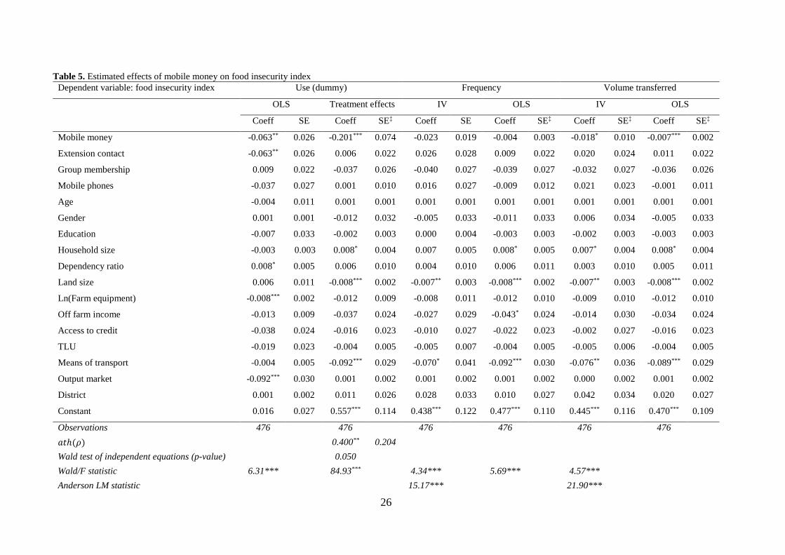
5.3.2.2. Effect of mobile money on binary food insecurity
Last but not least, we estimated a number of probit and IV probit models to obtain the effects of
different specifications of the treatment variable on binary food insecurity. The results are shown
in Table 6. In the IV probit specifications, we used the size of the exchange social network and
mobile phone network connectivity as instruments. The Wald tests of independent equations are
insignificant in all IV probit specifications indicating the absence of selection bias. We therefore
interpret probit estimates shown in columns 2, 6 and 10.
In line with the estimation in the previous section, we find that the use of mobile money has a
significant and negative effect. The adoption of mobile money reduces the likelihood of being food
insecure by ten percentage points (column 2). Also in line with previous estimation results, the
frequency of using mobile money does not have a significant effect on food insecurity. Finally, the
volume of money transferred is associated with a negative and significant effect. A one-unit
increase in the volume of money transferred via mobile phone reduces the probability of food
insecurity by 1.2 percentage points. The other control variables are consistent across the different
specifications of the treatment variable. Group membership has a negative and significant effect on
binary food insecurity, reducing the likelihood to be food insecure by about twelve percentage
points across all specifications. The variables land size and means of transport are negative and
significant, suggesting that larger land holdings and the ownership of a means of transport reduce
the likelihood of being food insecure. These findings are also consistent with the models on the
food insecurity index presented in the previous section.
29
Table 6. Estimated effects of mobile money on binary food insecurity
*, **, *** indicates the corresponding average marginal effects are significant at 10%, 5%, and 1% levels, respectively. ‡ Robust standard errors are reported. Marginal effects are
for discrete change of dummy variable from 0 to 1. Only second stage IV probit estimates are shown.
Use (dummy) Frequency Volume transferred
Probit IV probit Probit IV probit Probit IV probit
AME SE‡ Coef SE AME SE‡ Coef SE AME SE‡ Coef SE
Mobile money -0.104* 0.055 -0.679 0.784 -0.002 0.007 -0.015 0.114 -0.012** 0.005 -0.028 0.061
Extension contact 0.054 0.046 0.170 0.133 0.049 0.047 0.143 0.163 0.058 0.047 0.156 0.138
Group membership -0.116** 0.053 -0.309* 0.164 -0.116** 0.053 -0.328** 0.158 -0.117** 0.053 -0.332** 0.160
Mobile phones 0.001 0.024 0.067 0.144 -0.013 0.024 -0.023 0.160 0.007 0.024 0.012 0.133
Age 0.000 0.002 0.000 0.005 0.000 0.002 0.001 0.005 0.000 0.002 0.001 0.005
Gender -0.028 0.068 -0.044 0.200 -0.036 0.067 -0.096 0.192 -0.025 0.069 -0.072 0.198
Education -0.003 0.006 -0.004 0.018 -0.004 0.006 -0.008 0.026 -0.003 0.006 -0.008 0.017
Household size 0.012 0.010 0.032 0.026 0.013 0.010 0.034 0.026 0.012 0.010 0.034 0.026
Dependency ratio 0.001 0.023 -0.002 0.059 0.002 0.023 0.004 0.060 -0.000 0.023 0.000 0.060
Land size -0.011* 0.006 -0.027* 0.016 -0.011** 0.006 -0.030 0.018 -0.010* 0.006 -0.029* 0.016
Ln(Farm equipment) -0.027 0.020 -0.069 0.057 -0.026 0.020 -0.070 0.062 -0.025 0.020 -0.070 0.058
Off farm income -0.075 0.049 -0.149 0.181 -0.087* 0.049 -0.229 0.169 -0.069 0.050 -0.196 0.174
Access to credit 0.001 0.050 0.038 0.151 -0.007 0.050 -0.013 0.153 0.007 0.050 0.013 0.155
TLU -0.031** 0.013 -0.087** 0.039 -0.031** 0.013 -0.084** 0.040 -0.032** 0.013 -0.087** 0.040
Means of transport -0.216*** 0.073 -0.520** 0.210 -0.224*** 0.073 -0.567** 0.236 -0.211*** 0.073 -0.555*** 0.201
Output market 0.004 0.005 0.008 0.013 0.005 0.005 0.013 0.013 0.004 0.005 0.011 0.013
District 0.078 0.055 0.272 0.193 0.061 0.055 0.178 0.190 0.086 0.055 0.227 0.199
Observations 476 476 476
Wald statistic 70.11*** 63.89*** 63.47*** 58.92*** 73.02*** 59.64***
Pseudo R-square 0.111 0.11 0.12
Wald test of exogeneity (Prob > chi2) 0.62 0.93 0.95

30
6. Conclusion and policy implications
Our present study complements and adds to the limited literature on the broader welfare effects of
mobile money on households in developing countries. Using original household survey data, we
analysed the effect of mobile money on food security among rural households in Uganda.
Endogenous treatment effects and instrumental variables regressions are employed to control for
potential selection bias. We estimate several specifications of the treatment variable (use of mobile
money, frequency of use, volume transferred) as well as of the outcome variable (food
expenditures, food insecurity index, binary food insecurity). Our results are largely consistent
across the different model specifications indicating that the use of mobile money technology
positively contributes to enhancing household food security.
Regarding food expenditures per AE, we find that the use of mobile money, the frequency of use
and the volumes transferred are associated with increases in food expenditures. Furthermore, the
use of mobile money and the volumes transferred reduce subjectively perceived food insecurity,
both measured on a continuous scale as well as on a binary scale. The use of mobile money
increases food expenditures per AE by nine percentage points and reduces the food insecurity index
by 0.20 index points (one fifth of the standard deviation). The incremental effect of the frequency
of use is less important in the context of the subjective perception of food insecurity, but increases
food expenditures per AE: a one-unit increase in frequency is associated with a 1.9 percentage
point increase in food expenditures per AE. Furthermore, a one-percentage point increase in the
volumes transferred via mobile phone increases food expenditures per AE by one percentage point
and reduces perceived food insecurity by about 0.007 index points.
These results have important food policy implications, in particular that mobile money services can
play a role in improving food security among rural households in developing countries. Providing
households with access to cheap and easily available banking functions can have positive liquidity
effects and thus increase food expenditures and perceived food security. Against this background,

31
policy interventions to improve household food security should also consider the promotion of
mobile money and financial access among rural households in developing countries as a promising
strategy.
Besides mobile money, other covariates were found to be significantly associated with improved
food security. In particular, land size and ownership of a means of transport are consistently
significant across the different food expenditure and food insecurity specifications. These findings
have important policy implications as well. Due to land scarcity in Uganda, land area expansion is
not a feasible strategy. Instead, policy makers should focus on promoting the adoption of
sustainable intensification practices among rural households in Uganda. Sustainable intensification
practices that aim to increase output per unit of input resource while conserving the natural resource
base include for example modern high-yielding varieties, crop rotation, and soil and water
conservation practices (Smith, 2013; The Montpellier Panel, 2013). Finally, the positive effect of
ownership of a means of transport on food security is likely due to lower transaction costs and
enhanced access to input and output markets. In particular, in rural areas in Uganda (and other
developing countries) road infrastructure and public transport are poorly developed. Against this
background, public investments in the improvement of transport networks is likely to have positive
"side" effects on food security in rural areas.

32
References
Adams, R.H., Cuecuecha, A., 2013. The Impact of Remittances on Investment and Poverty in
Ghana. World Development 50, 24–40. 10.1016/j.worlddev.2013.04.009.
Barrett, C.B., 2010. Measuring Food Insecurity. Science 327 (5967), 825–828.
10.1126/science.1182768.
Becker, G.S., 1982. A Theory of Social Interactions. Journal of Political Economy 82 (6), 1063–
1093.
Bezu, S., Kassie, G.T., Shiferaw, B., Ricker-Gilbert, J., 2014. Impact of Improved Maize
Adoption on Welfare of Farm Households in Malawi: A Panel Data Analysis. World
Development 59, 120–131. 10.1016/j.worlddev.2014.01.023.
Coates, J., Swindale, A., Bilinsky, P., 2007. Household Food Insecurity Access Scale (HFIAS)
for measurement of food access: Indicator guide. Food and Nutrition Technical Assistance
Project (FANTA), Academy for Educational Development, Washington, DC.
Cock, N., D’Haese, M., Vink, N., Rooyen, C.J., Staelens, L., Schönfeldt, H.C., D’Haese, L.,
2013. Food security in rural areas of Limpopo province, South Africa. Food Sec. 5 (2), 269–
282. 10.1007/s12571-013-0247-y.
de Haen, H., Klasen, S., Qaim, M., 2011. What do we really know? Metrics for food insecurity
and undernutrition. Food Policy 36 (6), 760–769. 10.1016/j.foodpol.2011.08.003.
Deaton, A., Zaidi, S., 2002. Guidelines for constructing consumption aggregates for welfare
analysis. World Bank, Washington, DC, 104 pp.
Donovan, K., 2012. Mobile Money for Financial Inclusion, in: Information and Communications
for Development 2012. The World Bank, pp. 61–73.
Dupas, P., Robinson, J., 2013. Savings Constraints and Microenterprise Development: Evidence
from a Field Experiment in Kenya. American Economic Journal: Applied Economics 5 (1),
163–192. 10.1257/app.5.1.163.
FAO, 1996. The Rome Declaration on World Food Security. The World Food Summit, FAO,
Rome.
Field, A.P., 2013. Discovering statistics using IBM SPSS statistics: And sex and drugs and
rock'n'roll, 4th ed. SAGE, Los Angeles, Calif. [u.a.], XXXVI, 915 S.
IFC, 2011. Mobile Money Study: Summary Report. International Finance Corporation,
Washington, DC.
Jack, W., Ray, A., Suri, T., 2013. Transaction Networks: Evidence from Mobile Money in
Kenya. American Economic Review 103 (3), 356–361. 10.1257/aer.103.3.356.
Jack, W., Suri, T., 2014. Risk Sharing and Transactions Costs: Evidence from Kenya's Mobile
Money Revolution. American Economic Review 104 (1), 183–223. 10.1257/aer.104.1.183.
Kabunga, N.S., Dubois, T., Qaim, M., 2014. Impact of tissue culture banana technology on farm
household income and food security in Kenya. Food Policy 45, 25–34.
10.1016/j.foodpol.2013.12.009.
Karlan, D., Ratan, A.L., Zinman, J., 2014. Savings by and for the poor: a research review and
agenda. The Review of income and wealth 60 (1), 36–78. 10.1111/roiw.12101.
Kassie, M., Jaleta, M., Mattei, A., 2014a. Evaluating the impact of improved maize varieties on
food security in Rural Tanzania: Evidence from a continuous treatment approach. Food Sec. 6
(2), 217–230. 10.1007/s12571-014-0332-x.
Kassie, M., Ndiritu, S.W., Stage, J., 2014b. What Determines Gender Inequality in Household
Food Security in Kenya? Application of Exogenous Switching Treatment Regression. World
Development 56, 153–171. 10.1016/j.worlddev.2013.10.025.
Keino, S., Plasqui, G., van den Borne, Bart, 2014. Household food insecurity access: a predictor
of overweight and underweight among Kenyan women. Agric Food Secur 3 (1), 2.
10.1186/2048-7010-3-2.
Kikulwe, E.M., Fischer, E., Qaim, M., 2014. Mobile money, smallholder farmers, and household
welfare in Kenya. PLoS ONE 9 (10), e109804. 10.1371/journal.pone.0109804.

33
Kirui, O.K., Okello, J.J., Njiraini, G.W., 2013. Impact of mobile phone-based money transfer
services in agriculture: evidence from Kenya. Quarterly Journal of International Agriculture
52 (2), 141–162.
Kirui, O.K., Okello, J.J., Nyikal, R.A., 2012. Determinants of use and intensity of use of mobile
phone-based money transfer services in smallholder agriculture: case of Kenya. Paper
prepared for the International Association of Agricultural Economists (IAAE) Triennial
Conference, Foz do Iguaçu, Brazil, 18-24 August, 2012.
Mabiso, A., Cunguara, B., Benfica, R., 2014. Food (In)security and its drivers: insights from
trends and opportunities in rural Mozambique. Food Security 6 (5), 649–670.
10.1007/s12571-014-0381-1.
Maertens, A., Barrett, C.B., 2013. Measuring Social Networks' Effects on Agricultural
Technology Adoption. American Journal of Agricultural Economics 95 (2), 353–359.
10.1093/ajae/aas049.
Maxwell, D., Vaitla, B., Coates, J., 2014. How do indicators of household food insecurity
measure up? An empirical comparison from Ethiopia. Food Policy 47, 107–116.
10.1016/j.foodpol.2014.04.003.
McKenzie, D.J., 2005. Measuring inequality with asset indicators. Journal of Population
Economics 18 (2), 229–260. 10.1007/s00148-005-0224-7.
Miyata, S., Minot, N., Hu, D., 2009. Impact of Contract Farming on Income: Linking Small
Farmers, Packers, and Supermarkets in China. World Development 37 (11), 1781–1790.
10.1016/j.worlddev.2008.08.025.
Munyegera, G.K., Matsumoto, T., 2014. Mobile Money, Rural Household Welfare and
Remittances: Panel Evidence from Uganda. National Graduate Institute for Policy Studies,
Japan, National Graduate Institute for Policy Studies, Tokyo Japan.
Sahn, D.E., Stifel, D.C., 2000. Poverty Comparisons Over Time and Across Countries in Africa.
World Development 28 (12), 2123–2155. 10.1016/S0305-750X(00)00075-9.
Shiferaw, B., Kassie, M., Jaleta, M., Yirga, C., 2014. Adoption of improved wheat varieties and
impacts on household food security in Ethiopia. Food Policy 44, 272–284.
10.1016/j.foodpol.2013.09.012.
Sinyolo, S., Mudhara, M., Wale, E., 2014. Water security and rural household food security:
empirical evidence from the Mzinyathi district in South Africa. Food Security 6 (4), 483–499.
10.1007/s12571-014-0358-0.
Smith, P., 2013. Delivering food security without increasing pressure on land. Global Food
Security 2 (1), 18–23. 10.1016/j.gfs.2012.11.008.
StataCorp, 2013. Stata: Release 13. Statistical Software. StataCorp, College Station, TX:
StataCorp LP.
Storck, H., 1991. Farming systems and farm management practices of smallholders in the
Haraghe Highlands: A baseline survey. Wiss.-Verl. Vauk, Kiel, VI, 195 S ;
The Montpellier Panel, 2013. Sustainable Intensification: A New Paradigm for African
Agriculture, Imperial College London, London.