Global three-dimensional optimal disturbances in the Blasius

J. Fluid Mech., page 1 of 34 c© Cambridge University Press 2010

doi:10.1017/S0022112009993703

1

Global three-dimensional optimal disturbancesin the Blasius boundary-layer flow using

time-steppers

ANTONIOS MONOKROUSOS, ESPEN AKERVIK,LUCA BRANDT† AND DAN S. HENNINGSON

Linne Flow Centre, KTH Mechanics, SE-100 44 Stockholm, Sweden

(Received 12 May 2009; revised 27 November 2009; accepted 27 November 2009)

The global linear stability of the flat-plate boundary-layer flow to three-dimensionaldisturbances is studied by means of an optimization technique. We consider both theoptimal initial condition leading to the largest growth at finite times and the optimaltime-periodic forcing leading to the largest asymptotic response. Both optimizationproblems are solved using a Lagrange multiplier technique, where the objectivefunction is the kinetic energy of the flow perturbations and the constraints involvethe linearized Navier–Stokes equations. The approach proposed here is particularlysuited to examine convectively unstable flows, where single global eigenmodes of thesystem do not capture the downstream growth of the disturbances. In addition, the useof matrix-free methods enables us to extend the present framework to any geometricalconfiguration. The optimal initial condition for spanwise wavelengths of the order ofthe boundary-layer thickness are finite-length streamwise vortices exploiting the lift-upmechanism to create streaks. For long spanwise wavelengths, it is the Orr mechanismcombined with the amplification of oblique wave packets that is responsible for thedisturbance growth. This mechanism is dominant for the long computational domainand thus for the relatively high Reynolds number considered here. Three-dimensionallocalized optimal initial conditions are also computed and the corresponding wavepackets examined. For short optimization times, the optimal disturbances consist ofstreaky structures propagating and elongating in the downstream direction withoutsignificant spreading in the lateral direction. For long optimization times, we find theoptimal disturbances with the largest energy amplification. These are wave packetsof Tollmien–Schlichting waves with low streamwise propagation speed and fasterspreading in the spanwise direction. The pseudo-spectrum of the system for realfrequencies is also computed with matrix-free methods. The spatial structure of theoptimal forcing is similar to that of the optimal initial condition, and the largestresponse to forcing is also associated with the Orr/oblique wave mechanism, howeverless so than in the case of the optimal initial condition. The lift-up mechanism ismost efficient at zero frequency and degrades slowly for increasing frequencies. Theresponse to localized upstream forcing is also discussed.

† Email address for correspondence: [email protected]

2 A. Monokrousos, E.�

Akervik, L. Brandt and D. S. Henningson

1. IntroductionThe flat-plate boundary layer is a classic example of convectively unstable flows;

these behave as broadband amplifiers of incoming disturbances. As a consequence, aglobal stability analysis based on the asymptotic behaviour of single eigenmodes ofthe system will not capture the relevant dynamics. From this global perspective, allthe eigenmodes are damped, and one has to resort to an input/output formulation inorder to obtain the initial conditions yielding the largest possible disturbance growthat any given time and the optimal harmonic forcing. To do this, an optimizationprocedure is adopted. The aim of this work is to investigate the global stability of theflow over a flat plate subject to external perturbations and forcing and to examinethe relative importance of the different instability mechanisms at work. The approachadopted here can be extended to any complex flow provided a numerical solver forthe direct and adjoint linearized Navier–Stokes equations is available.

Recently, the global stability of the spatially evolving Blasius flow subject totwo-dimensional disturbances has been studied within an optimization frameworkby projecting the system onto a low-dimensional subspace consisting of dampedTollmien–Schlichting (TS) eigenmodes (Ehrenstein & Gallaire 2005). These resultswere extended by Akervik et al. (2008), who found that by not restricting the spannedspace to include only TS modes, the optimally growing structures could exploit boththe Orr and the TS wave packet mechanism and yield a substantially higher energygrowth. The Orr mechanism (Orr 1907) was studied in the context of parallel shearflows using the Orr–Sommerfeld/Squire (OSS) equations by Butler & Farrell (1992),who termed it the Reynolds stress mechanism. This instability extracts energy fromthe mean shear by transporting momentum down the mean momentum gradientthrough the action of the perturbation Reynolds stress. In other words, disturbancesthat are tilted against the shear can borrow momentum from the mean flow whilerotating with the shear until they are aligned with it. This mechanism is also referredto as wall-normal non-normality.

From the local point of view, the TS waves appear as unstable eigenvalues of theOrr–Sommerfeld equation. In the global framework, however, the global eigenmodesbelonging to the TS branch are damped (Ehrenstein & Gallaire 2005), and theevolution of TS waves consists of cooperating global modes that produce wavepackets. Considering the model problem provided by the Ginzburg–Landau equationwith spatially varying coefficients, Cossu & Chomaz (1997) demonstrated that thenon-normality of the streamwise eigenmodes resulting from the local convectiveinstabilities leads to substantial transient growth. This non-normality is revealed bythe streamwise separation of the direct and adjoint global modes induced by the basicflow advection; it is therefore also termed streamwise non-normality (Chomaz 2005).

It is now well established that when incoming disturbances exceed a certainamplitude threshold, the flat-plate boundary layer is likely to undergo transitiondue to three-dimensional instabilities arising via the lift-up effect (Ellingsen & Palm1975; Landahl 1980). This transient growth scenario, where streamwise vortices inducestreamwise streaks by the transport of the streamwise momentum of the mean flow,was studied for a variety of shear flows in the locally parallel assumption (cf. Butler& Farrell 1992; Reddy & Henningson 1993; Trefethen et al. 1993). The extensionto the non-parallel flat-plate boundary layer was performed at the same time byAndersson, Berggren & Henningson (1999) and Luchini (2000) by considering thesteady linear boundary-layer equations parabolic in the streamwise direction. In theseinvestigations, the optimal upstream disturbances are located at the plate leading edge

Optimal disturbances in the Blasius boundary-layer flow 3

and a Reynolds-number-independent growth was found for the evolution of streaksat large downstream distances. Levin & Henningson (2003) examined variations ofthe position at which disturbances are introduced and found the optimal locationto be downstream of the leading edge. In this study, low-frequency perturbationswere also considered, which are still within the boundary-layer approximation. Inthe global framework, an interpretation of the lift-up mechanism is presented e.g. byMarquet et al. (2008): Whereas the TS mechanism is governed by a transport of thedisturbances by the base flow, the lift-up mechanism is governed by a transport of thebase flow by the disturbances. Inherent in the lift-up mechanism is the component-wise transfer of momentum from the two cross-stream to the streamwise velocitycomponent (component-wise non-normality).

The standard way of solving the optimization problems involved in thedetermination of optimal initial condition (or forcing) is to directly calculate the matrixnorm of the discretized evolution operator (or the pseudo-spectrum of the resolvent)of the system. In the local approach, in which the evolution is governed by the OSSequations, it is clearly feasible to directly evaluate the matrix exponential or to invertthe relevant matrix. In the global approach, it is in general difficult, and in somecases impossible, to build the discretized system matrix. One possible remedy is tocompute a set of global eigenmodes with iterative methods and project the flowsystem onto the subspace spanned by these eigenvectors. The optimization is thenperformed in a low dimensional model of the flow: results for the flat-plate boundarylayer can be found in Ehrenstein & Gallaire (2005) and Akervik et al. (2008), whereastwo-dimensional and three-dimensional studies on separated flows were performed byAkervik et al. (2007), Gallaire, Marquillie & Ehrenstein (2007), Ehrenstein & Gallaire(2008), Marquet et al. (2008), Marquet et al. (2009) and Alizard, Cherubini & Robinet(2009).

However, the direct matrix-free approach followed here is preferable, if notindispensable, for more complicated flows. This amounts to solving eigenvalueproblems using only direct numerical simulations (DNSs) of the evolution operators.This approach is commonly referred to as a time-stepper technique (Tuckerman &Barkley 2000); one of its first applications was to the linear stability analysis of aspherical Couette flow (Marcus & Tuckerman 1987a ,b; Mamun & Tuckerman 1995).The time-stepper technique was then generalized to optimal growth calculations byintroducing the adjoint evolution operator and solving the eigenvalue problem ofthe composite operator (Blackburn, Barkley & Sherwin 2008; Barkley, Blackburn& Sherwin 2008) for backward-facing step flow; it was subsequently applied to theflat-plate boundary-layer flow subject to two-dimensional disturbances of Bagheriet al. (2009a).

Thus, in this paper we study the stability of the flat-plate boundary-layer flowsubject to three-dimensional disturbances from a global perspective using a time-stepper technique. The base flow has two inhomogeneous directions, namely thewall-normal and streamwise, thereby allowing a decoupling of Fourier modes inthe spanwise direction only. Both optimal initial condition and optimal forcing aretherefore first considered for a range of spanwise wavenumbers, seeking to find thespanwise scale of the most amplified disturbances. In the case of optimal initialconditions, we optimize over a range of final times, whereas time-periodic optimalforcing is computed for a range of frequencies. In addition, we compute for the firsttime optimal initial conditions localized in space. The evolution of the resulting wavepacket is analysed in terms of flow structures and propagation speed.



Whereas the computation of optimal initial condition is known in the global time-stepper context (see references above), the formulation of the optimal forcing problemin this framework is novel. This enables us to compute the pseudo-spectrum of thenon-normal governing operator with a matrix-free method. The latter type of analysiscan have direct implications for flow control as well: The optimization procedureallows us to determine the location and frequency of the forcing to which the flowunder consideration is most sensitive.

The paper is organized as follows. Section 2 is devoted to the description of thebase flow and the governing linearized equations. Sections 3 and 4 describe theLagrange approach to solving the optimization problems defined by the optimalinitial conditions and optimal forcing, respectively. The main results are presented in§ 5; the paper ends with a summary of the main findings.

2. Basic steady flow, governing equations and adjoint systemWe investigate the stability of the classical spatially evolving two-dimensional

flat-plate boundary-layer flow subject to three-dimensional disturbances. Thecomputational domain starts at a distance x from the leading edge defined by theReynolds number Rex = U∞x/ν =3.38 · 105 or Reδ∗ =1.72

√Rex = U∞δ∗

0/ν = 103. HereU∞ is the uniform free stream velocity, δ∗ is the local displacement thickness and ν isthe kinematic viscosity. We denote the displacement thickness at the inflow positionby δ∗

0 . All variables are non-dimensionalized by U∞ and δ∗0 . We solve the linearized

Navier–Stokes equations using a spectral DNS code described by Chevalier et al.(2007) on a domain Ω =[0, Lx] × [0, Ly] × [0, Lz]. The non-dimensional height of thecomputational box is Ly = 30 and the length is Lx =1000, and the spanwise width isLz = 502.6 for the case of localized initial conditions or defined in each simulation bythe Fourier mode under investigation. In the wall-normal direction y, a Chebyshev-tau technique with ny =101 polynomials is used along with homogeneous Dirichletconditions at the wall and the free-stream boundary. In the streamwise and spanwisedirections, we assume periodic behaviour, hence allowing for a Fourier transformationof all variables. For the simulations presented here, the continuous variables areapproximated by nx = 768 and nz = 128 Fourier modes in the streamwise and spanwisedirections, respectively, whereas we solve for each wavenumber separately in thespanwise direction when considering spanwise periodic disturbances, a decouplingjustified by the spanwise homogeneity of the base flow. Because the boundary-layer flow is spatially evolving, a fringe region technique is used to ensure that theflow is forced back to the laminar inflow profile at x = 0 (Nordstrom, Nordin &Henningson 1999). The fringe forcing quenches the incoming perturbations and isactive at the downstream end of the computational domain, x ∈ [800, 1000], sothat x = 800 can be considered as the effective outflow location, corresponding toRex = 1.138 × 106. The steady state used in the linearization is obtained by marchingthe nonlinear Navier–Stokes equations in time until the norm of the time derivative ofthe solution is numerically zero. Thus, the two-dimensional steady state with velocitiesU = (U (x, y), V (x, y), 0)T and pressure �(x, y) differs slightly from the well-knownBlasius similarity solution.

2.1. The linearized Navier–Stokes equations

The stability characteristics of the base flow U =(U (x, y), V (x, y), 0)T tosmall perturbations u = (u(x, t), v(x, t), w(x, t))T are determined by the linearized


Navier–Stokes equations

∂t u + (U · ∇) u + (u · ∇) U = −∇π + Re−1Δu + g, (2.1)

∇ · u = 0, (2.2)

subject to initial condition u(x, t = 0) = u0(x). Note that we have included adivergence-free forcing term g = g(x, t) to enable us to also study the responseto forcing as well as to initial condition. In the expression above, the fringe forcingterm is omitted for simplicity (see Bagheri, Brandt & Henningson 2009b).

When performing a systematic analysis of the linearized Navier–Stokes equations,we are interested in the initial condition u(0) and in the features of the flow statesu(t) at times t > 0. We will also consider the spatial structure of the time-periodicforcing g that creates the largest response at large times, that is when all transientseffects have died out. Our analysis will therefore consider flow states induced byforcing or initial conditions, where a flow state is defined by the three-dimensionalvelocity vector field throughout the computational domain Ω at time t . To this end,it is preferable to rewrite the equations in a more compact form. In order to doso, we define the velocities as our state variable, i.e. u = (u, v, w)T. Following Kreiss,Lundbladh & Henningson (1994), the pressure can be formally written in terms ofthe velocity field π = Ku, the solution to the equation

Δπ = −∇ · ((U · ∇)u + (u · ∇)U). (2.3)

The resulting state space formulation of (2.1) reads

(∂t − A)u − g = 0, u(0) = u0. (2.4)

Alternatively, A may also be defined using semi-group theory, in which it is referredto as the infinitesimal generator of the evolution operator T(t) (Trefethen & Embree2005), where T is defined as the operator that maps a solution at time t0 to timet0 + t

u(t + t0) = T(t)u(t0). (2.5)

In what follows we use the evolution operator T to study both the response toinitial condition and the regime response to forcing, i.e. we look at the long-termperiodic response. Indeed, for practical numerical calculations, the variables are oftendiscretized, so that the governing operator becomes a matrix of size n × n, withn= 3nxnynz for general three-dimensional disturbances. When considering spanwiseperiodic disturbances, we can focus on one wavenumber at a time and the dimension ofthe system matrix is reduced to n= 3nxny . However, even in this case the evaluation ofthe discretized evolution operator T = exp(At) is computationally not feasible. Thecomplete stability analysis, including the optimization, can be efficiently performed bymarching in time the linearized Navier–Stokes equations using a numerical code. Thisso-called time-stepper technique has indeed become increasingly popular in stabilityanalysis (Tuckerman & Barkley 2000).

2.2. Choice of norm and the adjoint equations

In order to measure the departure from the base flow, we use the kinetic energy ofthe perturbations

‖u(t)‖2 = (u(t), u(t)) =

∫Ω

uH u dΩ. (2.6)

Because the transition in shear flows is initiated by secondary instabilities induced bylocal gradients in the flow, one could alternatively use an infinity norm or maximize



directly the shear or vorticity. Using the above inner product, we may define theaction of the adjoint evolution operator as

(v, exp(At)u) = (exp(A†t)v, u), (2.7)

where A† is defined by the initial value problem

−∂tv = A†v = (U · ∇)v − (∇U)Tv + Re−1Δv + ∇Zv, v(T ) = vT . (2.8)

The adjoint system (2.8) is derived using the inner product in time space domainΣ = [0, T ] × Ω . The operator Z is the counterpart of the operator K for theadjoint pressure: σ = Zv. This initial value problem has a stable integration directionbackwards in time, so we may define the adjoint solution at time T − t for the forwardrunning time t as

v(T − t) = exp(A†t)vT , t ∈ [0, T ]. (2.9)

It is important to note that the addition of the forcing term g in (2.1) has no effecton the derivation of the adjoint equations. In particular, the fringe forcing term isself-adjoint because it is proportional to the velocity u.

3. Optimal initial conditionsIn this section, we derive the system whose solution yields initial conditions that

optimally excite flow disturbances. When seeking the optimal initial condition, weassume that the forcing term g in (2.4) is zero. We wish to determine the unitnorm initial condition u(0) yielding the maximum possible energy (u(T ), u(T )) at aprescribed time T . A common way of obtaining the optimal initial condition is torecognize that the condition

G(t) = max‖u(0)‖�=0

‖u(T )‖2

‖u(0)‖2= max

‖u(0)‖�=0

(u(0), exp(A†T ) exp(AT )u(0))

(u(0), u(0))(3.1)

defines the Rayleigh quotient of the composite operator exp(A†T ) exp(AT ). Theoptimization problem to be solved is hence the eigenvalue problem

γ u(0) = exp(A†T ) exp(AT )u(0). (3.2)

In the case of a large system matrix, as in fluid-flow systems, this eigenvalue problemcan be efficiently solved by matrix-free methods using a time-stepper (DNS) andperforming power iterations or the more advanced Arnoldi method (cf. Nayar &Ortega 1993; Lehoucq, Sorensen & Yang 1997); both methods only need a randominitial guess for u(0) and a numerical solver to determine the action of exp(AT ) andexp(A†T ) (Barkley et al. 2008).

One alternative approach relies on the Lagrange multiplier technique, which webelieve allows for more flexibility in defining different objective functions as well as inenforcing additional constrains. Here, we show how this approach is used to computethe unit norm initial condition u(0) non-zero only within a fixed region in space,Λ ⊂ Ω , i.e. the localized optimal initial condition. The objective is still maximizingthe kinetic energy at final time T

J = (u(T ), u(T )). (3.3)

The following constraints need to be enforced: the flow needs to satisfy the governinglinearized Navier–Stokes equations (2.4) (without forcing) and the initial condition


must have unit norm and exist only inside Λ. Additionally, the optimal perturbationmust be divergence-free. Hence, the Lagrange function reads

L(u, v, γ ) = (u(T ), u(T )) −∫ T

0

(v, (∂t − A) u) dτ

− γ ((u(0), u(0))Λ − 1) − (ψ, ∇ · u(0))Λ, (3.4)

where v, γ and ψ are the Lagrange multipliers. The inner product defined by (·, ·)Λcorresponds to an integral in Λ. Note that the normalization condition selects aunique solution to the eigenvalue problem and thus enables the numerical procedureto converge. We need to determine u, u(0), u(T ), v and γ such that L is stationary, anecessary condition for first-order optimality. This can be achieved by requiring thatthe variation of L is zero,

δL =

(∂L∂u

, δu)

+

(∂L∂v

, δv

)+

(∂L∂γ

)δγ +

(∂L∂ψ

)δψ = 0. (3.5)

This is only fulfilled when all terms are zero simultaneously. The variation with respectto the costate variable (or adjoint state variable) yields directly the state equation

(∂t − A)u = 0, (3.6)

and similarly the variation with respect to multiplier γ yields a normalization criterion(∂L∂γ

, δγ

)⇒ (u(0), u(0))Λ = 1. (3.7)

In order to take the variations with respect to the other variables, we performintegration by parts on the second term of L in (3.4) to obtain

L = (u(T ), u(T )) −∫ T

0

(u, (−∂t − A†) v) dτ − (v(T ), u(T ))

+ (v(0), u(0)) − γ ((u(0), u(0))Λ − 1) − (ψ, ∇ · u(0))Λ. (3.8)

The variation of this expression with respect to the state variable u yields an equationfor the adjoint variable as well as two optimality conditions(

∂L∂u

, δu)

⇒ −∫ T

0

(δu, (−∂t − A†)v) + (δu, v − γ u)|t=0 + (δu, u − v)|t=T = 0. (3.9)

The simplest choice to satisfy this condition is that each of these terms is zeroseparately

(−∂t − A†)v = 0, (3.10)

and

u(0) = γ −1v(0),

v(T ) = u(T ).

}(3.11)

Variations with respect to the initial velocity field give the following condition:

(δu(0), v(0)) − γ (δu(0), u(0))Λ − (δu(0), ∇ψ)Λ = 0. (3.12)

The above expression can be rewritten in integral form∫Ω−Λ

(δu(0)Tv(0)) +

∫Λ

δu(0)T(v(0) − γ u(0) − ∇ψ) = 0. (3.13)



The first integral is zero for δu(0) = 0, which implies that the initial condition is notupdated outside Λ. Therefore, the new guess for the localized initial condition u(0) is

u(0) = γ −1(v(0) − ∇ψ)|Λ. (3.14)

In the above, the scalar field ψ is obtained by combining (3.14) with

∂L∂ψ

= ∇ · u(0) = 0. (3.15)

This gives a projection to a divergence-free space where the pressure-like scalar field ψ

is solution to a Poisson equation. It can be proved that this is a unique projection. Inour numerical implementation, the projection is actually performed by transformingin the velocity–vorticity formulation adopted for the computations (Chevalier et al.2007).

The procedure described above solves an eigenvalue problem similar to (3.2) withthe addition of an operator PC that localizes in space and projects to a divergence-freespace

γ u(0) = PC exp(A†T ) exp(AT )u(0). (3.16)

The optimality system to be solved is hence composed of (3.6), (3.7), (3.10) and(3.11) along with the projection to divergence-free space (3.14). From (3.7) and thefirst relation in (3.11), it can be readily seen that γ = (v(0), v(0)). The remainingequations are solved iteratively as follows.

Starting with an initial guess u(0)n:(i) we integrate (3.6) forward in time and obtain u(T );(ii) v(T ) = u(T ) is used as an initial condition at t = T for the adjoint system (3.10),

which if integrated backward in time gives v(0);(iii) we determine a new initial guess by localizing v(0), casting it to a divergence-

free space and normalizing it to unit norm, u(0) = γ −1(v(0) − ∇ψ)|Λ;(iv) if |u(0)n+1 − u(0)n| is larger than a given tolerance, the procedure is repeated.Before convergence is obtained, u(0) and v(0) are not aligned. At convergence, u(0)

is an eigenfunction of (3.16). The iteration scheme above can be seen as a poweriteration scheme finding the largest eigenvalue of the problem (3.16). Because thecomposite operator is symmetric, its eigenvalues are real and its eigenvectors forman orthogonal basis. The eigenvalues of the system rank the set of optimal initialconditions according to the output energy at time T . If several optimals are sought,e.g. to build a reduced order model of the flow, the sequence of u(0)n produced in theiteration can be used to build a Krylov subspace suitable for the Arnoldi method.

4. Optimal forcingThis section focuses on the regime response of the system to time-periodic forcing.

Thus, we assume zero initial conditions, u(0) = 0, and periodic behaviour of theforcing function, i.e.

g = � ( f (x) exp(iωt)) , f ∈ �, ω ∈ �, (4.1)

where f defines the spatial structure of the forcing, ω is its circular frequency and �denotes the real part. With these assumptions, the governing equations become

(∂t − A)u − � ( f exp(iωt)) = 0, u(0) = 0. (4.2)

In this case, we wish to determine the spatial structure and relative strength of thecomponents of the forcing f that maximize the response of the flow at the frequency


ω in the limit of large times, i.e. the regime response of the flow. The measure of theoptimum is also based on the energy norm. Note that for this method to convergeand for the regime response to be observed, the operator A must be globally stable.In the spatial framework, this requirement is always satisfied.

In order to formulate the optimization problem, it is convenient to work in thefrequency domain, thereby removing the time dependence. By assuming time-periodicbehaviour, u is replaced by the complex field u so that

u = � (u exp(iωt)) . (4.3)

The resulting governing equations can then be written as

(iωI − A)u − f = 0. (4.4)

Note that the operator A, containing only spatial derivatives, remains unchanged.The Lagrange function for the present optimization problem is similar in structure tothat used to determine the optimal initial condition and is formulated as follows:

L(u, v, γ, f ) = (u, u) − (v, (iωI − A)u − f ) − γ (( f , f ) − 1) . (4.5)

The objective function is the disturbance kinetic energy of the regime response (u, u),where the complex variable u requires the use of the Hermitian transpose. Theadditional constrains require the flow to be the solution to the linearized forcedNavier–Stokes equations and introduce a normalization condition for the forcingamplitude. Because the state variable u is a solution to the time-independent system(4.4), the inner product used in the definition of the adjoint involves only spatialintegrals. The time behaviour of the costate or adjoint variable is also assumed to beperiodic v = �(v exp(iωt)). Thus, in the derivation of the adjoint, the time derivativeis replaced by the term iωu, with adjoint −iωv. As for the computation of the optimalinitial condition, we take variations with respect to u, v, f and γ :

δL =

(∂L∂ u

, δu)

+

(∂L∂ v

, δv

)+

(∂L∂ f

, δ f)

+

(∂L∂γ

)δγ. (4.6)

The first-order optimality condition requires all of the terms to be simultaneouslyzero. By taking variations with respect to the costate variable (or adjoint variable),we again obtain the state equation (4.4). Similarly, the variation with respect to themultiplier γ yields the normalization criterion ( f , f ) − 1 =0. In order to take thevariations with respect to the other variables, we perform integration by parts onthe second term of L in (4.5) to obtain

L(u, v, γ, f ) = (u, u) − (u, (−iωI − A†)v) + ( f , v) − γ (( f , f ) − 1) . (4.7)

No initial–final condition terms appear during this integration by parts because herethe inner product is only in space (in contrast to the optimal initial condition).Variations with respect to the state variable u and to the forcing function f yield(

∂L∂ u

)⇒ u − (−iωI − A†)v = 0, (4.8)

(∂L∂ f

)⇒ f = γ −1v. (4.9)

Equations (4.4) and (4.8) are the two equations that we have to solve with thetime-stepper. The normalization condition ( f , f ) = 1 and (4.9) provide the optimality



condition that is used to calculate the new forcing field after each iteration of theoptimization loop.

Below, we show the equivalence between the Lagrange multiplier technique and thecorresponding standard matrix method when the resolvent norm is considered. Theformal solution to (4.2) can be written as

u = (iωI − A)−1 f . (4.10)

The corresponding solution for the adjoint system is

v = (−iωI − A†)−1u. (4.11)

Combining the two equations above and using (4.9),

f =1

γ(−iωI − A†)−1(iωI − A)−1 f . (4.12)

This is a new eigenvalue problem defining the spatial structure of the optimal forcingat frequency ω that is solved iteratively; the largest eigenvalue corresponds to thesquare of the resolvent norm

γ = ‖(iωI − A)−1‖2. (4.13)

Note that the actual implementation uses a slightly different formulation becausethe available time-stepper does not solve directly (4.4) and (4.8). In practice, thegoverning equations are integrated in time long enough that the transient behaviourrelated to the system operator A has died out. The regime response for the directand adjoint system is extracted by performing a Fourier transform of the velocityfield during one period of the forcing.

The steps of the optimization algorithm therefore are the follows:(i) Integrate (4.2) forward in time and obtain the Fourier transform response u at

the frequency of the forcing.(ii) Here u is used as a forcing for the adjoint system.(iii) A new forcing function is determined by normalizing f n+1 = v/γ .(iv) If | f n+1 − f n| is larger than a given tolerance, the procedure is repeated.We will also study localized optimal forcing; see § 5.2.2. The derivation of the

optimality conditions is similar to that presented for spatially localized perturbationsin § 3 and are not reported here.

A validation of the method is presented in figure 1, where the results from thepresent adjoint-based iteration procedure are compared with those obtained by thestandard method of performing a singular value decomposition (SVD) of the resolventof the Orr–Sommerfeld and Squire equations for the parallel Blasius flow (cf. Schmid& Henningson 2001). In figure 1(a), the response to forcing with spanwise wavenumberβ = 0 is shown for different frequencies, whereas the response to steady forcing withstreamwise wavenumber α is shown in figure 1(b). In the latter case, variations of thespanwise wavenumbers are considered. In both cases, excellent agreement betweenthe two methods is observed.

5. ResultsThe flat-plate boundary-layer flow is globally stable, i.e. there are no eigenvalues

of A located in the unstable half-plane. Hence, we do not expect to observe theevolution of single eigenmodes. In Akervik et al. (2008), the non-modal stability ofthis flow subject to two-dimensional disturbances was studied by considering the


0.01 0.02 0.03 0.04 0.05 0.060

100

200

300

400

500

600

700

ω

G

0.2 0.4 0.6 0.8 1.00

2000

4000

6000

8000

10 000

β

(a) (b)

Figure 1. Comparison of results from the adjoint iteration scheme (circles) and direct solutionin terms of SVD of the OSS resolvent (solid lines) for optimal forcing to the parallel Blasius flowat Re = 1000. (a) Zero spanwise wavenumber β for different frequencies ω and for streamwisewavenumber α = 0.1. (b) Streamwise wavenumber α = 0.1 for different spanwise wavenumbersβ subject to forcing with frequency ω = 0.05. Both plots show excellent agreement betweenthe two methods. Note that in order to obtain a regime response in the parallel case, thewavenumbers are chosen so that the system operator is stable.

optimal superposition of eigenmodes. These authors found that the optimal initialcondition exploits the well-known Orr mechanism to efficiently trigger the propagatingTS wave packet. In Bagheri et al. (2009a), the stability of the same flow was studiedusing forward and adjoint iteration scheme together with the Arnoldi method toreproduce the same mechanism. By allowing for three-dimensional disturbances, it isexpected that in addition to the instability mechanisms mentioned above (convectiveTS instability and the Reynolds stress mechanism of Orr), the lift-up mechanism willbe relevant in the system.

This has been well understood both using the OSS equations (Butler & Farrell1992; Reddy & Henningson 1993) in the parallel temporal framework and usingthe parabolized stability equations in the spatial non-parallel framework (Anderssonet al. 1999; Luchini 2000; Levin & Henningson 2003). In the former formulation,the base flow is assumed to be parallel. At the Reynolds number Re = 1000, theinflow Reynolds number of the present investigation, it is found that for spanwisewavenumbers β larger than ≈ 0.3, there is no exponential instability of TS/obliquewaves. The largest non-modal growth due to the lift-up mechanism is observed atthe wavenumber pair (α, β) = (0, 0.7). In this work, we do not restrict ourselves tozero streamwise wavenumber α = 0, but instead take into account the developing baseflow. Indeed, the spatially developing base flow allows for transfer of energy betweendifferent wavenumbers through the convective terms.

5.1. Optimal initial condition

5.1.1. Spanwise periodic flows

We investigate the potential for growth of initial conditions with different spanwisewavenumbers β by solving the eigenvalue problem (3.2) for a range of instances oftime T . As explained above, this amounts to performing a series of direct and adjointnumerical simulations until convergence towards the largest eigenvalues of (3.2) isobtained.

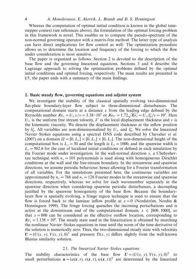
Figure 2(a) shows the energy evolution when optimizing for different times andspanwise wavenumber β = 0.55. It is at this wavenumber that the maximum growth



0 500 1000 1500 2000100

102

104

t t

E

0 200 400 60010–1

100

101

102

r.m

.s

urms

vrms

wrms

(a) (b)

Figure 2. (a) Energy evolution of the optimal initial conditions for different times T at thewavenumber β =0.55, where the optimal streak growth is obtained. The largest growth isobtained at time T = 720. The maximum at each time in this figure defines the envelopegrowth. (b) Component-wise r.m.s. values when optimizing for time T = 720. A transfer ofenergy from the wall-normal and spanwise component to the streamwise velocity is observedduring the time evolution, clearly showing that the lift-up mechanism is active.

due to the lift-up mechanism is found for the configuration under consideration. Fromfigure 2(b) it is evident that the disturbance leading to the maximum streak growthat time T = 720 exploits the component-wise transfer between velocity componentsinherent to the lift-up mechanism. The initial condition is in fact characterized bystrong wall-normal v and spanwise w perturbation velocity while the flow at latertimes is perturbed in its streamwise velocity component.

An important feature of this high-Reynolds-number flat-plate boundary-layer flowwith length Lx = 800 is that the combined Orr/Tollmien–Schlichting mechanism isvery strong with a growth potential of γ1 = 2.35 × 104 (see also Bagheri et al. 2009a)for time T = 1800. If, however, the streaks induced by the lift-up mechanism havereached sufficiently large amplitudes to trigger significant nonlinear effects, the TSwave transition scenario will be bypassed. In figure 3, a contour map of the maximumgrowth versus optimization time and spanwise wavenumbers β is shown. Note thatlocal maxima are obtained in two regions: (i) a low spanwise wavenumber regimedominated by the TS/oblique waves where the growth is the largest but slow and(ii) for high spanwise wavenumber, it is the fast lift-up mechanism that is dominating.The TS/oblique mechanism can be seen to yield one order of magnitude largergrowth than the lift-up instability. The global maximum growth is obtained at thewavenumber β = 0.05 and not for β = 0. This somewhat surprising result can beexplained by the larger initial transient growth of spanwise-dependent perturbationswhich initiates the TS-waves. The growth rate of TS-waves is almost independent ofβ for the low values under consideration (see e.g. figure 3.10 of Schmid & Henningson2001).

The competition between the exponential and algebraic growth was also studiedusing local theory by Corbett & Bottaro (2000). These authors have shown thatas the Reynolds number increases, the growth due to modal instability becomesmore pronounced. The results presented in that work for Reθ = 386 (equivalentto Reδ∗ = 1000 in our scaling) indicate that TS instability becomes dominant forfinal times T > 2000. Our results show that in a spatially evolving boundary layerwith local Reynolds number Reδ∗ ranging between 1000 and 1800, the exponentialgrowth dominates at times larger than about 1250. In the following, we study in


23

23

23

74

74

74

74

215

215

215

215

599

599

599

599599

1995

1995

1995

19951995

1995 1995

5011

5011

18738

t

β

Energy amplification

500 1000 1500 20000

0.1

0.2

0.3

0.4

0.5

0.6

0.7

0.8

Figure 3. Contour map of optimal growth due to initial condition in the time spanwisewavenumber domain. The contour levels span three orders of magnitude and thus we usea logarithmic scale. The values on the contours indicate the energy growth correspondingto that line. The maximum streak growth is obtained for β = 0.55 at time T =720 and theamplification factor is G = 2.63 × 103. The global maximum is obtained for β =0.05 at timeT = 1820, with the streamwise exponential amplification of oblique waves combined with theOrr mechanism. The amplification factor is G = 2.71 × 104.

more detail the disturbances corresponding to the two local maxima mentionedabove.

The evolution of the most dangerous initial condition is shown in figure 4.The streamwise velocity component of the optimal initial condition leading to themaximum growth at time T = 1820 is depicted together with the flow response atvarious times. The initial disturbance is the same as in the two-dimensional caseleaning against the shear of the base flow (see figure 4a). The resulting instabilityexploits the Orr mechanism to efficiently initialize the wave packet propagation,eventually giving the disturbance shown in figure 4(b–d ).

Figure 5 shows the space–time diagram for the evolution of the three velocitycomponents of the disturbance. Isocontours of the integrated, in the spanwiseand wall-normal directions, root-mean-square (r.m.s.) values associated with eachcomponent are plotted versus the streamwise direction and time. Because this isa global view of local modal instability, there is no significant component-wisetransfer of energy, and thus the different components of the disturbance evolve(grow) in a similar manner. Weak interactions between the components can be dueto non-parallel effects. Additionally, the propagation velocity of the disturbance isestimated from the space–time diagrams by tracking the edges of the disturbance.These edges are defined as the point where the r.m.s. values have amplitude 1 %of the local peak value. (All the propagation velocities presented will be measuredin this way.) The leading edge of the wave packet travels at cle = 0.51 whereasthe trailing edge has a velocity cte = 0.33. These values show remarkable agreementwith the classic results on the propagation of wave packets by Gaster (1975) andGaster & Grant (1975).



5

(a)

0 100 200 300 400 500 600 700 800

100 200 300 400 500 600 700 800

100 200 300 400 500 600 700 800

100 200 300 400 500 600 700 800

500

–50

5

(b)

0 500

–50

5

(c)

0 500

–50

5

(d)

0 500

–50

Figure 4. Isosurfaces of streamwise component of disturbances at the spanwise wavenumberβ =0.05. Red/blue colour signifies isosurfaces corresponding to positive/negative velocitiesat 10% of the maximum. (a) Streamwise component of optimal initial condition leading tothe global optimal growth at time T = 1820. (b–d ) Corresponding flow responses at timesT = 400, 1000 and 1600.

The optimal initial condition leading to the maximum growth at time T = 720 forspanwise wavenumber β = 0.55 and the corresponding flow response at various timesare shown in figure 6. The initial disturbance is an elongated perturbation with most ofits energy (99.94 %) in the wall-normal and spanwise velocity components (figure 6a).The resulting instability exploits the lift-up eventually giving the disturbance shownin figure 6(b–e). This is a result of local non-modal instability characterized by thestrong transfer of energy from the wall-normal and spanwise towards the streamwisevelocity component. The wall-normal velocity component is shown in figure 6(b) tosuggest that the Orr mechanism is active here as well; it delays the final decay of thestreamwise vortices so that they can induce streaks more effectively. Already at timet = 100 more than 99 % of the kinetic energy of the perturbation is in the streamwisecomponent. As can be seen, the disturbance evolves into alternating slow and fastmoving streaks that are tilted so that the leading edge is higher than the trailing edgeas observed in the experimental investigation by Lundell & Alfredsson (2004).

Note that although the optimal initial condition is streamwise independent forparallel flows, it is localized in the streamwise direction for a spatially growingboundary layer. This indicates that it is most efficient to extract energy from themean flow farther upstream where non-parallel effects are stronger. For optimizationtimes longer than that of the peak value, still with β = 0.55, the initial perturbationis located farther upstream and is shorter. This is to compensate for the downstreampropagation of perturbations out of the control domain. Conversely, for optimizationtimes lower than T = 720, the initial conditions assume more and more the form of a


x

Tim

eu

0 200 400 600 800

200

400

600

800

1000

1200

1400

1600

x

v

0 200 400 600 800

200

400

600

800

1000

1200

1400

1600

x

Tim

e

w

0 200 400 600 800

200

400

600

800

1000

1200

1400

1600

(a) (b)

(c)

Figure 5. Spatio-temporal diagram of the three velocity components of the perturbation forthe TS-wave case (optimization time is T = 720) (a streamwise, b wall normal and c spanwise).The propagation velocity of the leading edge of the disturbance is cle = 0.51 whereas that of thetrailing edge is cte = 0.33.

packet of vortices aligned in the streamwise direction and tilted upstream. The growthis then due to a combined Orr and lift-up mechanism.

The space–time diagram for each velocity component of the streaky optimalperturbation is presented in figure 7. The non-modal nature of the instability and thecomponent-wise transfer of energy are seen in the plots. The streamwise componentis for large times several orders of magnitude larger than that for the other two. Thepropagation velocity of the disturbance is calculated: the leading-edge velocity of the‘streak-packet’ is cle = 0.87 whereas the trailing edge travels at velocity cte =0.44. Notethat these values are based on the streamwise velocity component. The propagationvelocities of the non-modal streaks are larger than those of modal disturbances. Thiscan be explained by the fact that the disturbances are located in the upper partof the boundary layer, especially in the downstream part, as also deduced from thethree-dimensional visualization in figure 6. Note, finally, in the plot for the spanwisevelocity component a kink around t = 400 and x =400. In this region, the maincontribution to the trailing edge of the disturbance changes from streamwise vorticesto streamwise streaks. The propagation velocity of streamwise vortices is thus largerthan that of the streaks as confirmed by the reduced slope of the peak contours infigures 7(a) and 7(b).

To further interpret the present results, we perform a Fourier transform along thestreamwise direction of the two disturbances investigated above and compute the



5

(a)

0 100 200 300 400 500 600 7005

0–5

5

(b)

0 100 200 300 400 500 600 7005

0–5

5

(c)

0 100 200 300 400 500 600 700 50

–5

5

(d)

0 100 200 300 400 500 600 700 50

–5

5

(e)

0 100 200 300 400 500 600 700

800

800

800

800

800 50

–5

Figure 6. Evolution of streamwise velocity when initializing the system with the optimalinitial condition at β = 0.55. (a) The wall-normal velocity of the optimal initial condition.(b) The wall-normal velocity at t = 200 with surface levels at 10 % of its maximum value.(c) The streamwise velocities at t = 200, (d ) t = 400 and (e) t = 600. The optimization time isT = 720.

energy distribution in the various streamwise wavenumbers α (the energy densityis first integrated in the wall-normal and spanwise directions). The result shownin figure 8 demonstrates that the TS-wave disturbance has a peak at a relativelyhigher α ≈ 0.17, a value in agreement with predictions from local parallel stabilitycalculations. The streak mode, conversely, has most of its energy at the lowestwavenumbers.

Four different optimal initial conditions for β = 0.55 and T = 720 are shown infigure 9. The wall-normal velocity component of the eigenvector leading to themaximum growth is reported in 9(a). Because the base flow is uniform in thespanwise direction, the second eigenvector has the exact same shape as the first,only shifted half a wavelength in z as shown in figure 9(b). These eigenvectorscorrespond to the same eigenvalue γ1,2 = 2.6 × 103, and they may be combined linearlyto obtain a disturbance located at any spanwise position. In figure 9(c,d ), the thirdeigenvector associated with γ3 = 2.2 × 103 and the fifth eigenvector associated withγ5 = 1.6 × 103 are shown, respectively. These eigenvectors also come in pairs withmatching eigenvalues. It is thus possible by the Arnoldi method to obtain severaloptimals for a single parameter combination. This has not been done previously for


x

Tim

eu

200 400 600 8000

100

200

300

400

500

600

x

v

w

200 400 600 8000

100

200

300

400

500

600

x

Tim

e

200 400 600 8000

100

200

300

400

500

600

(a) (b)

(c)

Figure 7. Spatio-temporal diagram of the three velocity components of the perturbation forthe streak case (optimization time is T = 720) (a streamwise, b wall normal and c spanwise).The propagation velocity of the leading edge of the disturbance is cle = 0.87 whereas that of thetrailing edge is cte = 0.44. The two speeds are measured in the second half of the time domainafter the initial transient phase.

0 0.1 0.2 0.3 0.410–2

10–1

100(a)

(b)

TS-wave

E

10–4

10–2

100

E

0 0.1 0.2 0.3 0.4

Streak

α

Figure 8. Energy spectra along the streamwise direction for the optimal initial condition atT = 1820, β = 0.05 (TS-wave) and T = 720, β =0.55 (streak).

the Blasius flow, although Blackburn et al. (2008) computed several optimals for theflow past a backward-facing step.

The responses to each of these initial conditions are shown in figure 9(e–i ). One cansee that the sub-optimal initial conditions reproduce structures of shorter extension



5(a)

0

0

–5

5

5(b)

0–5

5(c)

0–5

5(d)

0–5

0 100 200 300 400 500 600 700 800

0

50 100 200 300 400 500 600 700 800

0

50 100 200 300 400 500 600 700

0

50 100 200 300 400 500 600 700

800

800

5(e)

0

0

–5

5

5(f )

0–5

5(g)

0–5

5(h)

0–5

0 100 200 300 400 500 600 700 800

0

50 100 200 300 400 500 600 700 800

0

50 100 200 300 400 500 600 700

0

50 100 200 300 400 500 600 700

800

800

Figure 9. Wall-normal component of the leading four eigenvectors for the optimizationproblem at β = 0.55, t = 720 and the corresponding responses. The structures are plotted overone wavelength in the spanwise direction. Red/blue colour indicate isosurfaces correspondingto positive/negative velocities at 10 % of the maximum. (a) The initial condition with largestgrowth. (b) Flow structures corresponding to the second eigenvalue. This is a spanwise-shiftedversion of the first eigenvector. (c) Third eigenvector associated with the same eigenvalue asthe fourth eigenvector (not shown). (d ) Fifth eigenvector. In (e–g) and (i ), the correspondingresponses are shown, in particular the streamwise component. Note that the axes are not atthe actual aspect ratio: the structures are far more elongated.

200 400 6000

500

1000

1500

2000

2500

3000

t

E

Optimal 1

Sub-optimal 3

Sub-optimal 5

Sub-optimal 7

Figure 10. The evolution of the energy of the perturbation in time for each of the initialconditions in figure 9. The sub-optimals denoted by even number give the same evolution asthe corresponding perturbation with odd number.

and with low- and high-speed streaks alternating in the streamwise direction. Figure 10shows the energy evolution versus time for each of the sub-optimals. The energygrowth is similar in the beginning; however, later on, faster decay is observed withdecreasing order of optimality. Optimal perturbations form an orthogonal basis; thisfact may be exploited to project incoming disturbances and predict their evolution.

5.1.2. Localized optimal initial condition

In this section, we look into the general case of three-dimensional initial disturbancesusing the method described in § 3. A large domain is chosen to allow for a fully


Time Component Initial condition Response Total growth

u 0.00398 275.42913720 v 0.36452 0.02334 275.76202

w 0.63149 0.30954

u 0.74441 1012.395501820 v 0.00314 278.58122 1763.75695

w 0.25244 472.78022

Table 1. Energy of each component of the tree-dimensional optimal initial condition and thecorresponding response. The total energy amplification is reported in the last column. All thevalues are normalized with the total energy of the initial condition.

three-dimensional disturbance to propagate and expand in all directions withoutinteracting with the boundaries. The spanwise width is chosen to be Lz =502.6(corresponding to the fundamental wavenumber β = 0.0125) for the cases with longestoptimization time and Lz = 251.3 (β = 0.025) for the shorter optimization times.Furthermore, nz = 128 Fourier modes were used in the spanwise direction, instead offour for the spanwise periodic cases. This increases the total number of degrees offreedom in our optimization problem from approximately 1–30 million.

The initial condition is placed near the inflow of the computational domain andpower iterations are used to compute the optimal shape of the disturbance insidea fixed region. The area to which the initial condition is limited is 30δ∗

0 long and40δ∗

0 wide and it is centred around the location x =25δ∗0 and z = 0. Along the wall-

normal direction the optimization process restricts the perturbation near the wall,inside the boundary layer, hence no additional localization is adopted. The casespresented here correspond to the two physical mechanisms found to be relevant inthe previous section: the Orr/TS-wave scenario and the lift-up process. To excite thetwo separately, the corresponding optimization times are chosen to be T =1820 andT =720. In addition, one intermediate case, T = 900, where both these mechanismsare active, is presented.

For the longest optimization time considered (see figure 11), the TS-wave scenariocompletely dominates the dynamics. The characteristic upstream tilted structures arepresent in the initial condition and all the velocity components achieve a significantgrowth. The wave packet grows while travelling downstream and it consists ofstructures almost aligned in the spanwise direction, forming symmetric arches. Thethree-dimensional nature of this wave packet is noticeable in the spanwise velocitycomponent of the response, accounting for the spreading of the disturbance normalto the propagation direction and to the presence of unstable oblique waves. Asin the case of the spanwise periodic disturbances, the total energy growth due tothe streamwise normality (TS-waves for T = 1820) is about of one order magnitudelarger than the amplification triggered by the lift-up effect at T = 720 (component-wise non-normality). Table 1 compiles the energy amplifications for the cases underinvestigation and reports the value of the energy content in each velocity componentfor the initial and final conditions.

The flow structures shown in figure 12, with corresponding amplitudes in table 1,document the optimal initial conditions for T = 720. The lift-up effect with theformation of streamwise elongated streaks is evident in this case. The initialcondition is characterized by strong streamwise vorticity, wall-normal and spanwisevelocity components, whereas the response is predominantly in the streamwise



5

0

–200

0

(a)

200

0 100 200 300 400

u

v

w

500 700 800600

5

0

–200

0

(b)

200

0 100 200 300 400 500 700 800600

5

0

–200

0

(c)

200

0 100 200 300 400 500 700 800600

Figure 11. Optimal localized initial condition and corresponding response at time T = 1820,the optimal TS wave packet. The amplitudes of each velocity component are reported intable 1.

velocity component. Interestingly, we note weak TS-waves propagating behind thestreaks (visible in the wall-normal and spanwise velocity components). Because theoptimization time is short, TS-waves will not have the opportunity to grow and theircontribution to the initial condition is therefore limited. However, this cannot bezero for a localized initial perturbation. Note further that the spanwise componentis found to be weak and hence the spreading of the disturbance in this direction islimited.

The characteristics of the optimal wave packets are analysed by the space–timediagrams in figures 13 and 14. Here, the propagation of the disturbance in thestreamwise direction is determined by considering the integral of the energy associatedwith each velocity component in the wall-normal and spanwise directions. Similarly,the lateral spreading is computed by integrating the perturbation velocities in thestreamwise and wall-normal directions. Comparing the two cases we see that the TSwave packet expands faster in the spanwise direction while travelling downstreammore slowly than the optimal streaky wave packet. The propagation velocity of theleading edge of the TS-like disturbance is cle = 0.47 whereas the trailing edge travelsat cte = 0.32. The spanwise spreading speed is cz =0.084, corresponding to an angle ofθ = 11.46◦. These values can be compared to those observed experimentally by Gaster(1975) and Gaster & Grant (1975) and to the theoretical analysis of Koch (2002).Koch (2002) determined the propagation speed of the leading edge of a localized wavepacket to be 0.5 and the trailing-edge velocity to be 0.36 by computing the groupvelocity of three-dimensional neutral waves. The largest spanwise group velocity wasfound to be approximately 0.085, a value very close to those reported here. The


5

0

–50

0

(a)

50

0 100 200 300

u

v

w

400 500 700 800600

5

0

–50

0

(b)

50

0 100 200 300 400 500 700 800600

5

0

–50

0

(c)

50

0 100 200 300 400 500 700 800600

Figure 12. Optimal localized initial condition and corresponding response at time T = 720,the optimal streaky wave packet. The amplitudes of each velocity component are reported intable 1.

agreement is remarkable even though the results of Koch (2002) are obtained at alower Reynolds number, i.e. Re = 580.

The difference between leading and trailing edges of the optimal streaky wavepacket, cle = 0.90 and cte = 0.36, explains the larger extension of the latter; althoughthe front travels at the speeds typical of the upper part of the boundary layer where thestreaks are located, the trailing edge velocity is that of the unstable waves seen on therear. The spanwise spreading speed is cz =0.0098, corresponding to an angle ofθ =0.89◦. This spreading rate is that of the energetically dominant velocity component,i.e. the streamwise component. The slow lateral diffusion is most likely only due tothe effect of viscosity; the growing streaky structures are therefore characterized byzero spanwise propagation velocity.

Figures 14(b) and 14(c) clearly demonstrate the short and slower packet of wavesfollowing the main streaky structures. As mentioned above, the spanwise propagationof the streamwise vortices and streaks is limited; conversely, the sequence of waveson the rear part of the wave packet has a spanwise spreading rate comparable to thatof the TS wave packet, in particular the value cz =0.073 is obtained by consideringthe energy of the spanwise velocity component.

Finally, we computed optimal disturbances for intermediate optimization timeswhen amplifications are generally lower than those in the two previous cases. Fortimes around T = 800 to T =900 perturbations containing both streaky and wavystructures emerge. The spectrum of the initial conditions contains a broad range ofdisturbances, whereas the flow response is again characterized by short-wavelength



200

0 200 400x

600 800 0 200 400x

600 800 0 200 400x

u v w

u v w

600 800

–200 –100 0 100 200z

–200 –100 0 100 200z

–200 –100 0 100 200z

400

600

800

1000t

1200

1400

1600

1800

(a) (b) (c)

(d) (e) (f)

200

400

600

800

1000

1200

1400

1600

1800

200

400

600

800

1000

1200

1400

1600

1800

200

400

600

800

1000t

1200

1400

1600

1800

200

400

600

800

1000

1200

1400

1600

1800

200

400

600

800

1000

1200

1400

1600

1800

Figure 13. Spatio-temporal diagram of the integrated in the wall-normal direction of ther.m.s. values of three velocity components of the perturbation for the optimal TS wave-packet(optimization time T = 1820). (a–c) The spreading of the disturbance in the streamwise directionwhere the disturbance velocity is integrated in the spanwise and wall-normal directions: (a)streamwise, (b) wall-normal and (c) spanwise velocity components, respectively. (d–f ) Theevolution in the spanwise direction of the perturbations integrated in the streamwise andwall-normal directions. The propagation velocity of the leading edge of the disturbance iscle = 0.47 whereas that of the trailing edge is cte = 0.32. The spanwise spreading speed atsufficiently large times is cz = 0.084.

instability waves following elongated streaks. The TS wave packet becomes more andmore relevant as the optimization time increases.

5.2. Optimal forcing

5.2.1. Global forcing

Because boundary layers are convectively unstable, thereby acting as noiseamplifiers, a prominent role is played by the response to forcing, rather than bythe time evolution of the initial condition. The optimal forcing is therefore a relevantmeasure of the maximum possible growth that may be observed in the computationaldomain. Analysis of the frequency response can also have implications for controlrevealing the forcing location and frequencies to which the flow is most sensitive.Although the evolution of the optimal initial condition consists of the propagation


100

200

300

400

500

600

700

100

200

300

400

500

600

700

100

200

300

400

500

600

700

t

0 200 400x

600 800 0 200 400x

600 800 0 200 400x

600 800

u v w

u v w

(a) (b) (c)

100

200

300

400

500

600

700

100

200

300

400

500

600

700

100

200

300

400

500

600

700

t

(d) (e) (f)

–100 –50 0 50 100z

–100 –50 0 50 100z

–100 –50 0 50 100z

Figure 14. Spatio-temporal diagram of the integrated in the wall-normal direction of the r.m.s.values of three velocity components of the perturbation for the optimal streaky wave packet(optimization time T = 720). (a–c) The propagation of the disturbance in the streamwise dir-ection where the disturbance velocity is integrated in the spanwise and wall-normal directions:(a) streamwise, (b) wall-normal and (c) spanwise velocity components, respectively. (d–f )The evolution in the spanwise direction of the perturbations integrated in the streamwiseand wall-normal directions. The propagation velocity of the leading edge of the disturbanceis cle = 0.90 whereas that of the trailing edge is cte = 0.36. The spanwise spreading speed iscz = 0.0098 (based on the u component).

and amplification of a wave packet, eventually leaving the computational box (ormeasurement section), the response of the flow to periodic forcing will consist ofstructures with a fixed amplitude at each streamwise station, oscillating around themean flow. We investigate the structure of the optimal forcing and the correspondingresponse for a range of spanwise wavenumbers and frequencies. Thus, for eachwavenumber we examine a number of temporal frequencies. Ideally, we would liketo solve the linearized Navier–Stokes equations for very large times, ensuring thatwe are only considering the regime (long-time) response at the specific frequencyunder investigation. In practice, however, we are restricted to a finite final time bythe computational cost of solving the direct and adjoint equations involved in theiteration scheme. Using power iterations to find the largest eigenpair typically requiresfrom approximately 15 iterations to about 100 for the most stable frequencies; in



0.02 0.04 0.06 0.08 0.100

2

4

6

8

10

(× 104) (× 104)

ω β

G

0.2 0.4 0.6 0.8 1.0 1.20

1

2

3

4(a) (b)

Figure 15. (a) Frequency response for zero spanwise wavenumber i.e. two-dimensionaldisturbances. The optimal response is obtained for the frequency ω =0.055. (b) Responseto zero frequency forcing ω = 0 for different spanwise wavenumbers. The maximum response isobtained at β =0.6.

other words, we need to integrate the governing equations at least 30 times. As canbe deduced from the results in the previous section, transiently growing perturbationsof small spanwise scale leave our domain at time t ≈ 2000, while locally unstableTS-waves propagate at a speed of about 0.3 U∞. This observation, along with severalconvergence tests using different integration intervals to extract the flow regimeresponse, leads to the conclusion that integration to T = 5000 is long enough toobserve the pure frequency response.

Figure 15 shows the square of the resolvent norm, i.e. the response to forcing for thetwo limiting cases β = 0 and ω = 0. In figure 15(a), the response to two-dimensionalforcing, inducing perturbations with β = 0, is displayed. The maximum response isobserved for the frequency ω = 0.055. This maximum is obtained at the frequencywhere the least stable TS eigenvalue is located (see Bagheri et al. 2009a). Indeed, itis known that by projecting the dynamics of the flow onto the basis of eigenmodes,the response to forcing is given by the combination of resonant effects (distancein the complex plane from forcing frequency to eigenvalue) and non-modal effects,i.e. the cooperating non-orthogonal eigenvectors (Schmid & Henningson 2001). InAkervik et al. (2008) it was shown for a similar flow that non-normal eigenvectorscould induce a response about 20 times larger than that induced only by resonanteffects.

The response to zero temporal frequency for different spanwise wavenumbers β

is shown in figure 15(b), where according to local theory the maximum response isexpected for spanwise periodic excitations. The maximum growth may be observedfor the wavenumber β =0.6, a slightly larger value than that for the optimal initialcondition case. Note that in the case of optimal forcing there is a smaller differencein the maximum gain between the two different dominating mechanisms (TS-wavesversus streaks).

A full parameter study has been carried out in the frequency–spanwise wavenumber(ω, β) plane. A contour map showing the regime response to optimal forcing isdisplayed in figure 16. As in the case of the optimal initial condition, the globalmaximum response to forcing is observed for β = 0.05. It reaches this maximumfor the frequency ω = 0.055. A second region of strong amplification is found forlow frequencies and high spanwise wavenumbers. Here the most amplified structures


6458

6458

64

58

6458

12328

12328

12328

12328

12328

18650

18650

18650

1865018650

18650

28216

28216

28216

28216

28216

42687

42687

64580

64580

ω

β

Energy amplification

0.02 0.04 0.06 0.080

0.2

0.4

0.6

0.8

1.0

Figure 16. Contour map of response to forcing with frequency ω versus spanwise wavenumberβ . The contour levels span three orders of magnitude and thus we use a logarithmic scale. Thevalue on the contours indicates the energy growth corresponding to that line. The maximumresponse to forcing is observed for β = 0.05 and for the frequency ω = 0.055. The amplificationfactor is G = 1.01 × 105. The maximum growth due to the streak mechanism is found for thespanwise wavenumber β =0.6 at ω = 0 where the amplification factor is G = 3.45 × 104.

5

(a)

(b)5

0 500

–50

500

–50

100 200 300 400 500 600 700 800

0 100 200 300 400 500 600 700 800

Figure 17. Isosurfaces of optimal forcing and response for the streamwise wavenumberβ = 0.05 subject to forcing at the frequency ω = 0.055. Red/blue colour signifies isosurfacescorresponding to positive/negative velocities at 10% of the maximum. (a) Streamwisecomponent of optimal forcing structure. (b) Streamwise velocity component of the response.

consist of streamwise elongated streaks induced by cross-stream forcing. At the largestspanwise wavenumbers, we also observe that the decay of the amplification whenincreasing the forcing frequencies is rather slow. Conversely, the peak correspondingto excitation of the TS-waves is more pronounced.

A visualization of the overall maximum amplification, found for the spanwisewavenumber of β = 0.05 and for the same frequency ω = 0.55 yielding the optimaltwo-dimensional forcing, is presented below. The optimal forcing in the streamwisemomentum equation and the streamwise velocity component of the optimal responseare shown in figure 17. The optimal forcing structures lean against the shear (seefigure 17a) to optimally trigger the Orr mechanism; the regime long-time response ofthe flow, shown in figure 17(b), reveals the appearance of amplified TS-waves at thedownstream end of the computational domain.

The optimal forcing structure at β = 0.6 and the zero frequency has almost all itsenergy in the spanwise and wall normal components, that is the flow is forced



5(a)

0 5 0–5

100 200 300 400 500 600 700 800

5(b)

0 50

–5

100 200 300 400 500 600 700 800

5(c)

0 50

–5

100 200 300 400 500 600 700 800

Figure 18. Isosurfaces of optimal forcing and response for the streamwise wavenumberβ =0.6 subject to steady forcing. Red/blue colour indicates isosurfaces corresponding topositive/negative velocities at 10 % of the maximum. (a) Wall-normal component of optimalforcing structure. (b) Spanwise component of optimal forcing. (c) Streamwise velocitycomponent of the flow response. Both the forcing structures and the response are highlyelongated in the streamwise direction.

0 0.1 0.2 0.3 0.410–2

10–1

(a)

(b)

100TS-wave

0 0.1 0.2 0.3 0.4α

E

10–4

10–2

100

E

Streak

Figure 19. Energy spectra along the streamwise direction for the optimal forcing atω = 0.055, β =0.05 (TS-wave) and ω =0, β = 0.6 (streak).

optimally in the wall-normal and spanwise directions as shown, among others,by Jovanovic & Bamieh (2005) for channel flows. The wall-normal and spanwisecomponents of the forcing are displayed in figures 18(a) and 18(b). The r.m.s. valuesof the streamwise component of the forcing are only 2 % of that of its spanwise andwall-normal counterparts. The lift-up effect transfers momentum into the streamwisecomponent (shown in figure 18c), which contains 99.99 % of the energy of the flowresponse. The streak amplitude increases in the streamwise direction until the fringeregion is encountered.

The Fourier transform along the streamwise direction of the two disturbancesinvestigated above is shown in figure 19. As in the case of the optimal initialconditions in figure 8, the energy density is first integrated in the wall-normal andspanwise directions. The results indicate that the TS-wave disturbance has a peak ata relatively high α ≈ 0.17, whereas the zero-frequency forcing is concentrated at thelowest wavenumbers. The peak at the wavenumber of the most unstable TS-waves ismore evident in the case of forcing than in the case of the optimal initial condition(see figure 8).


0 200 400 600

102

104

106

E

x200 400 600

x

Full forcingLocalized forcing

0

500

1000

1500

2000

2500

3000

3500

Localized forcingParab. eq. final pointParab. eq. integral

(a) (b)

Figure 20. Downstream evolution of the kinetic energy of the flow integrated overcross-stream planes. In (a), blue and green lines are used to indicate the response to steadyforcing active everywhere in the domain (Full forcing) and in a short region near the inflow(localized forcing), respectively. The data are scaled with the magnitude of the forcing computedas integral over the whole domain. In (b), the blue line corresponds to the case of localizedforcing in (a), whereas green (Parab. eq. final point) indicates the evolution of the optimalinitial condition yielding the largest possible kinetic energy at the downstream location 662δ∗

0(Levin & Henningson 2003), and the red line (Parab. eq. integral) indicates the evolution ofoptimal initial condition yielding the largest integral over the streamwise domain. In order tomake a physically relevant comparison, we have scaled the data pertaining to the ‘localizedforcing’ with the value of the response just downstream of the forcing region. The centre ofthe forcing is at the location x = 32.3δ∗

0 corresponding to the optimal upstream location inLevin & Henningson (2003).

5.2.2. Localized forcing

In this section, we present results obtained by restricting the forcing to a smallregion near the inflow of the computational domain. The formulation presented in§ 4 is altered by multiplying the forcing f with a function λ(x) which is non-zero onlyin a short streamwise region. The edges of this region are defined by two smoothstep functions rising from zero to one over a distance of about 1δ∗

0 . The centre of theforcing is chosen to be at x = 23δ∗

0 with width of 4δ∗0 , if not otherwise stated.

This problem is physically closer to the case when disturbances are generatedupstream, closer to the leading edge, and their evolution is monitored as they areconvected downstream. Initially, a comparison with optimal upstream disturbancescalculated by means of the parabolized equations is thus presented (see results inLevin & Henningson 2003).

To this aim, we compute the optimal localized steady forcing for spanwisewavenumber β = 0.53 at x = 32.3δ∗

0 . These were found to be the location and spanwisescale of the overall optimal by Levin & Henningson (2003); in their scalings theycorrespond to X =0.37 and β =0.53 for an initial perturbation downstream ofthe leading edge with Reynolds-number-independent evolution, here assumed tobe Rex =106.

In figure 20, the streamwise growth of the energy of the perturbation obtainedwith four different approaches is shown. In figure 20(a), we compare the flow regimeresponse to steady forcing active everywhere in the domain with the response to forcinglocalized upstream. Furthermore, the localized forcing is compared in figure 20(b)with the evolution of the optimal initial conditions yielding the largest possible kineticenergy at the downstream location 662δ∗

0 and with the evolution of the optimal



| fi|

y

DNS

0.5 1.0

| fi|

0.5 1.0

| fi|

0.5 1.00

5

10

15

fu

fv

fw

Parab. eq. final point Parab. eq. integral(a)

0

5

10

15(b)

0

5

10

15(c)

fu

fv

fw

fu

fv

fw

Figure 21. Wall-normal profiles of the streamwise, spanwise and wall-normal componentsof (a) the optimal localized forcing (integrated in the streamwise direction), (b) the initialcondition yielding the largest possible kinetic energy at the downstream location 662δ∗

0 , (c)the initial condition yielding the largest integral of the disturbance energy over the streamwisedomain.

upstream velocity profile yielding the largest integral of the perturbation energy overthe whole streamwise domain (see also Cathalifaud & Luchini 2000). The two initialcondition problems here are computed with the parabolic stability equations (DavidTempelmann 2009, private communication); the case having as objective functionthe integral of the perturbation energy is indeed more relevant for comparison withthe present results. It can be seen that the growth is faster when the forcing is activeeverywhere in our control domain because the component-wise transfer of energyis at work at every streamwise position. The two curves obtained with the parabolicequations (figure 20a) are similar: faster growth is observed when the control optimizesover the whole domain, whereas a larger final level is reached when the objectiveis limited to the last downstream station. The comparison between the response to‘localized forcing’ and the ‘parabolic equations’ cases reveals good agreement. Themain differences between the two methods are the different set of equations and theway the disturbance is introduced. In Levin & Henningson (2003) and Cathalifaud &Luchini (2000), the linearized boundary-layer equations are used, whereas we use theNavier–Stokes equations. In addition, an optimal upstream boundary condition iscomputed by Levin & Henningson (2003), whereas an optimal forcing is sought here.

Figure 21(a) displays the structure of the optimal forcing function for the caseof localized excitation. The wall-normal profiles shown in the plot are obtained byintegrating the forcing in the streamwise direction. Figures 21(b) and 21(c) depictinstead the optimal initial condition obtained with the parabolic boundary-layerequations, i.e. a streamwise vortex pair. The structure of the disturbances is remarkablysimilar; in the case of the optimal forcing (figure 21a), the action is located closer tothe wall with a relatively weaker wall-normal component. While comparing the casesin figures 21(b) and 21(c), one can note that the vortices leading to the largest possibleenergy downstream are located farther up into the free stream. Conversely, when theperturbations are required to grow over the whole domain, the disturbance needs to


0 200 400 600 800

0.5

1.0

1.5

2.0

2.5

3.0

3.5(× 104) (× 104)

G

x

Response to steady localizedforcing for various β

0 0.2 0.4 0.6 0.8 1.0 1.2

0.5

1.0

1.5

2.0

2.5

3.0

3.5

Gm

ax

β

Maximum growth(a) (b)

Figure 22. (a) Streamwise evolution of the response to steady localized forcing for differentspanwise wavenumbers β . The arrow indicates increasing β . (b) Maximum response versusspanwise wavenumbers.

be located in the shear layer so that its effect can be readily felt (cf. figure 21a,c).The results in the figure indicate that forcing the momentum equation is less effectivein the free stream: optimal forcing thus induces streaks which grow for a shorterdownstream distance.

A parameter study is conducted to examine the effect of frequency and spanwisescale of the localized forcing. First, the results obtained when varying the spanwisewavenumber are shown (figure 22). The downstream evolution originating fromoptimal localized disturbances of zero frequency is displayed for the spanwisewavenumbers investigated. A slower energy growth is observed for the lowerwavenumbers owing to the lower forcing to the streaks (proportional to β); thewavenumber giving the largest peak response for the present configuration is β = 0.8.Forcing of smaller scales induces streaks rapidly, but viscous dissipation causes earlierdecay.

As shown by Andersson et al. (2001), among others, in the range of validity of theboundary layer equations, there is a coupling between the streamwise and spanwiselength scales of the disturbance. It is in fact possible to show that a streak familyu(x, y, z), defined by the spanwise wavenumber β0, is independent of the Reynoldsnumber. This results in a scaling property that couples the streamwise and spanwisescales, implying that the same solution is valid for every combination of the streamwiselocation x + x0 (distance from the leading edge) and of β such that their productstays constant. In other words, this amounts to moving along the plate and varyingthe spanwise wavenumber so that the local spanwise wavenumber β0δ

∗/δ∗0 remains

constant (see also Brandt et al. 2003). To further examine this scaling property, thestreamwise coordinate in figure 22(a) is multiplied by the spanwise wavenumber of thedisturbance and the result is shown in figure 23. Despite the fact that the streamwiseextent of each curve is different, the curves indicating the evolution of the streakydisturbance collapse notably, thus confirming the similarity of the boundary-layerstreaks.

Finally, we investigate the case of zero spanwise number (pure two-dimensionaldisturbances) and vary the temporal frequency. The results are shown in figure 24.The growth observed here is due to the combined Orr and TS-wave mechanism, and



100 200 300 4000

0.5

1.0

1.5

2.0

2.5

3.0

3.5(× 104)

G

β • x

Boundary-layer scaling

Figure 23. Streamwise evolution of the response to localized forcing for different spanwisewavenumbers β where the streamwise position x is scaled with β . The distance from theleading edge is considered to rescale the data.

0 200 400 600 800100

102

104

106

102

104

106

108

x

Response to 2D localized forcingfor various frequencies

0 0.02 0.04 0.06 0.08 0.10ω

Maximum growth

G

Gm

ax

(a) (b)

Figure 24. (a) Streamwise evolution of the response to localized forcing for different temporalfrequencies ω. The arrow indicates increasing ω. (b) Maximum growth with respect to ω. Thespanwise wavenumber is β =0.

thus the value of the optimal frequency is close to that obtained when forcing overthe whole domain, ω = 0.055. The structure of the optimal forcing for the frequencywith largest amplification is displayed in figure 25. The excitation is localized closerto the wall, well inside the boundary layer, when compared to the forcing formingstreamwise streaks; see figure 21. Forcing the streamwise momentum equation issignificantly more efficient at triggering the Orr mechanism and the subsequent wavepacket of two-dimensional TS-waves.

6. ConclusionsWe have used a Lagrange multiplier technique in conjunction with direct and

adjoint linearized Navier–Stokes equations in order to quantify the growth potential inthe spatially developing flat-plate boundary-layer flow at moderately high Reynolds.


0.2 0.4 0.6 0.8 1.00

5

10

15Forcing structure

| fi|

y

fu

fv

Figure 25. Localized forcing with frequency. We plot the streamwise and wall-normalcomponents of the forcing function. The quantities are integrated in the streamwise direction.Note that this is a two-dimensional structure, thus the spanwise component is zero.

Spanwise periodic and fully three-dimensional disturbances are investigated. Weconsider both the initial conditions leading to the largest possible energy amplificationat time T and the optimal spatial structure of time-periodic forcing. To the best ofour knowledge, the pseudo-spectrum of the governing operator along real frequenciesis computed here for the first time with matrix-free methods. The optimizationframework adopted does not restrict us to assume slow variation of the baseflow in the streamwise direction, common to both the first-order approximationof the OSS formulation and the more advanced parabolic stability equations (PSE)approximation. Specifically, we do not, as in the PSE framework, need differentequations to describe the lift-up instability and the wave packet propagation.

For the optimal initial condition we find that the largest potential for growth isfound at small spanwise wavenumbers and consists of upstream tilted structures,enabling the subsequent disturbances to exploit the Orr mechanism and the localconvective instability of the oblique wave packet of TS-waves. The length and positionof the initial disturbance is related to the final time of the optimization: short timeevolution requires the wave packet to be initiated farther downstream in the regionof largest local instability and vice versa for longer optimization times. The lift-upinstability mechanism inherent to spanwise wavelengths of the order of the boundary-layer thickness is faster than the Orr/oblique instability; for the present configuration,the streaks reach their maximum energy earlier; conversely, the TS-wave instabilityneeds more time to extract the same amount of energy, at the same time travellinga shorter distance. The evolution of the kinetic energy of these two perturbations intime and space is displayed in figure 26.

The results further indicate that streamwise vortices of finite length become optimalonce a spatially evolving boundary layer with inflow/outflow conditions is considered.As concerns the optimal response to periodic forcing, the difference in the twoinstabilities is less pronounced. In this case, the Orr/oblique wave instability onlymanages to gain a factor of two in energy more than the streak mechanism. The largestamplification of the local convective instability over the non-modal streak generationcan be explained by the long computational box examined and the relatively highinflow Reynolds number. Starting closer to the leading edge, one can expect streaksto become more relevant.



0 100 200 300 400 500 600 700

101

102

103

104

105

0 0

400

400 800

800

1200

1200

1600

1600

2000

2000

Position of disturbance

Ener

gy

TS-waveStreak

Figure 26. Evolution of the kinetic energy of the two optimal initial perturbations for t =720(streaks) and t = 1820 (TS-waves) versus the current spatial position. The position of thedisturbance is computed by tracking its ‘centre of mass’ using the kinetic energy as density.The numbers beside the markers correspond to time instances.

Three-dimensional localized optimal initial conditions are also computed and thecorresponding wave packets examined. For short optimization times, the optimaldisturbances consist of streaky structures propagating and elongating downstreamwithout any significant spreading in the lateral direction. For long optimization times,conversely, the optimal disturbances are characterized by wave packets of TS-waves.These travel at lower streamwise speed and with faster spreading in the spanwisedirection. The TS-wave packet can achieve the largest possible energy amplification.Intermediate optimization times are also considered where both the TS- and streakmechanisms are relevant. The wave packet has therefore features from both scenariospreviously considered: It consists of elongated streaks in the streamwise velocitycomponent, followed by short-wavelength instability waves, mainly evident in thecross-stream velocities.

Finally, we examine the effect of upstream disturbances on the boundary-layerflow. Thus, we introduce a localized forcing near the inflow of the computationalbox and compute the forcing structure that provides the largest response overour control domain. First, we compare with results based on the solution ofthe parabolized Navier–Stokes equations: good agreement is obtained despite thedifferences between the two methods. Second, we investigate zero-frequency upstreamforcing and show a maximum for perturbations with spanwise wavenumber largerthan that obtained when the forcing location is not constrained. Third, an analysisof time-periodic two-dimensional forcing is considered: the findings agree with thoseobtained with distributed forcing because the flow response corresponds in both casesto exponentially growing TS-waves at the forcing frequency.

Three different destabilizing mechanisms are considered in this study, all at work inthe boundary layer flow. Although these could be explained using the OSS equations,they are analysed without any simplifying assumptions. This work is of a more generalcharacter. By choosing an objective function and using the full linearized Navier–Stokes equations as constraints, we are not limiting ourselves to simple geometries.Whenever a DNS code is available to accurately describe a flow, all that is neededin order to investigate the stability characteristics is a linearized version of the


code and the implementation of the corresponding adjoint equations along with awrapper ensuring the correct optimization scheme. The method used here is thereforeapplicable to any geometrical configuration.

The authors wish to thank David Tempelmann for providing data from theparabolic stability equations and many fruitful discussions and Carlo Cossu forinspiring comments on the manuscript. Computer time provided by SNIC (SwedishNational Infrastructure for Computing) is gratefully acknowledged. This work issupported by the Swedish Research Council (VR).

REFERENCES

Akervik, E., Ehrenstein, U., Gallaire, F. & Henningson, D. S. 2008 Global two-dimensionalstability measures of the flat plate boundary-layer flow. Eur. J. Mech. B. Fluids 27, 501–513.

Akervik, E., Hœpffner, J., Ehrenstein, U. & Henningson, D. S. 2007 Optimal growth, modelreduction and control in a separated boundary-layer flow using global eigenmodes. J. FluidMech. 579, 305–314.

Alizard, F., Cherubini, S. & Robinet, J.-C. 2009 Sensitivity and optimal forcing response inseparated boundary layer flows. Phys. Fluids 21, 064108.

Andersson, P., Berggren, M. & Henningson, D. S. 1999 Optimal disturbances and bypasstransition in boundary layers. Phys. Fluids 11, 134–150.

Andersson, P., Brandt, L., Bottaro, A. & Henningson, D. S. 2001 On the breakdown of boundarylayers streaks. J. Fluid Mech. 428, 29–60.

Bagheri, S., Akervik, E., Brandt, L. & Henningson, D. S. 2009a Matrix-free methods for thestability and control of boundary layers. AIAA J. 47, 1057–1068.

Bagheri, S., Brandt, L. & Henningson, D. S. 2009b Input–output analysis, model reduction andcontrol of the flat-plate boundary layer. J. Fluid Mech. 620, 263–298.

Barkley, D., Blackburn, H. M. & Sherwin, S. J. 2008 Direct optimal growth analysis fortimesteppers. Intl J. Numer. Meth. Fluids 57, 1435–1458.

Blackburn, H. M., Barkley, D. & Sherwin, S. J. 2008 Convective instability and transient growthin flow over a backward-facing step. J. Fluid Mech. 608, 271–304.

Brandt, L., Cossu, C., Chomaz, J.-M., Huerre, P. & Henningson, D. S. 2003 On the convectivelyunstable nature of optimal streaks in boundary layers. J. Fluid Mech. 485, 221–242.

Butler, K. M. & Farrell, B. F. 1992 Three-dimensional optimal perturbations in viscous shearflow. Phys. Fluids A 4, 1637–1650.

Cathalifaud, P. & Luchini, P. 2000 Algebraic growth in boundary layers: optimal control byblowing and suction at the wall. Eur. J. Mech. B. Fluids 19, 469–490.

Chevalier, M., Schlatter, P., Lundbladh, A. & Henningson, D. S. 2007 A pseudo spectral solverfor incompressible boundary layer flows. Tech. Rep. Trita-Mek 7.

Chomaz, J. M. 2005 Global instabilities in spatially developing flows: non-normality andnonlinearity. Annu. Rev. Fluid Mech. 37, 357–392.

Corbett, P. & Bottaro, A. 2000 Optimal perturbations for boundary layers subject to streamwisepressure gradient. Phys. Fluids 12 (1), 120–130.

Cossu, C. & Chomaz, J. M. 1997 Global measures of local convective instability. Phys. Rev. Lett.77, 4387–90.

Ehrenstein, U. & Gallaire, F. 2005 On two-dimensional temporal modes in spatially evolvingopen flows: the flat-plate boundary layer. J. Fluid Mech. 536, 209–218.

Ehrenstein, U. & Gallaire, F. 2008 Two-dimensional global low-frequency oscillations in aseparating boundary-layer flow. J. Fluid Mech. 614, 315–327.

Ellingsen, T. & Palm, E. 1975 Stability of linear flow. Phys. Fluids 18, 487–488.

Gallaire, F., Marquillie, M. & Ehrenstein, U. 2007 Three-dimensional transverse instabilities indetached boundary layers. J. Fluid Mech. 571, 221–233.

Gaster, M. 1975 A theoretical model of a wave packet in a boundary layer over a flat plate. Proc.R. Soc. London, Ser. A 347, 271–289.



Gaster, M. & Grant, I. 1975 An experimental investigation of the formation and development ofa wave packet in a laminar boundary layer. Proc. R. Soc. London, Ser. A 347, 253–269.

Jovanovic, M. R. & Bamieh, B. 2005 Componentwise energy amplification in channel flows. J. FluidMech. 534, 145–183.

Koch, W. 2002 On the spatio-temporal stability of primary and secondary crossflow vortices in athree-dimensional boundary layer. J. Fluid Mech. 456, 85–111.

Kreiss, G., Lundbladh, A. & Henningson, D. S. 1994 Bounds for treshold amplitudes in subcriticalshear flows. J. Fluid Mech. 270, 175–198.

Landahl, M. T. 1980 A note on an algebraic instability of inviscid parallel shear flows. J. FluidMech. 98, 1–34.

Lehoucq, R. B., Sorensen, D. & Yang, C. 1997 Arpack users’ guide: solution of largescale eigenvalue problems with implicitly restarted Arnoldi methods. Tech. Rep. fromhttp://www.caam.rice.edu/software/ARPACK/, Computational and Applied Mathematics,Rice University.

Levin, O. & Henningson, D. S. 2003 Exponential vs algebraic growth and transition prediction inboundary layer flow. Flow Turbul. Combust. 70, 183–210.

Luchini, P. 2000 Reynolds-number-independent instability of the boundary layer over a flat surface:optimal perturbations. J. Fluid Mech. 404, 289–309.

Lundell, F. & Alfredsson, P. H. 2004 Streamwise scaling of streaks in laminar boundary layerssubjected to free-stream turbulence. Phys. Fluids 16 (5), 1814–1817.

Mamun, C. K. & Tuckerman, L. S. 1995 Asymmetry and Hopf bifurcation in spherical Couetteflow. Phys. Fluids 7 (1), 80–91.

Marcus, P. S. & Tuckerman, L. S. 1987a Simulation of flow between concentric rotating spheres.Part 1. Steady states. J. Fluid Mech. 185, 1–30.

Marcus, P. S. & Tuckerman, L. S. 1987b Simulation of flow between concentric rotating spheres.Part 2. Transitions. J. Fluid Mech. 185, 31–65.

Marquet, O., Lombardi, M., Chomaz, J. M., Sipp, D. & Jacquin, L. 2009 Direct and adjoint globalmodes of a recirculation bubble: lift-up and convective non-normalities. J. Fluid Mech. 622,1–21.

Marquet, O., Sipp, D., Chomaz, J. M. & Jacquin, L. 2008 Amplifier and resonator dynamicsof a low-Reynolds-number recirculation bubble in a global framework. J. Fluid Mech. 605,429–443.

Nayar, M. & Ortega, U. 1993 Computation of selected eigenvalues of generalized eigenvalueproblems. J. Comput. Phys. 108, 8–14.

Nordstrom, J., Nordin, N. & Henningson, D. S. 1999 The fringe region technique and the Fouriermethod used in the direct numerical simulation of spatially evolving viscous flows. SIAMJ. Sci. Comp. 20, 1365–1393.

Orr, W. M. F. 1907 The stability or instability of the steady motions of a perfect liquid and of aviscous liquid. Part I: A perfect liquid. Part II: A viscous liquid. Proc. R. Irish Acad. A 27,9–138.

Reddy, S. C. & Henningson, D. S. 1993 Energy growth in viscous channel flows. J. Fluid Mech.252, 209–238.

Schmid, P. J. & Henningson, D. S. 2001 Stability and Transition in Shear Flows . Springer.

Trefethen, L. N., Trefethen, A. E., Reddy, S. C. & Driscoll, T. A. 1993 Hydrodynamic stabilitywithout eigenvalues. Science 261, 578–584.

Trefethen, N. & Embree, M. 2005 Spectra and Pseudospectra: The Behaviour of Nonnormal Matricesand Operators . Princeton University Press.

Tuckerman, L. S. & Barkley, D. 2000 Bifurcation analysis for timesteppers. In Numerical Methodsfor Bifurcation Problems and Large-Scale Dynamical Systems , pp. 453–566. Springer.

Documents

Global three-dimensional optimal disturbances in the Blasius